Embedded Nonlocal Operator Regression (ENOR): Quantifying model error in learning nonlocal operators
Abstract
Nonlocal, integral operators have become an efficient surrogate for bottom-up homogenization, due to their ability to represent long-range dependence and multiscale effects. However, the nonlocal homogenized model has unavoidable discrepancy from the microscale model. Such errors accumulate and propagate in long-term simulations, making the resultant prediction unreliable. To develop a robust and reliable bottom-up homogenization framework, we propose a new framework, which we coin Embedded Nonlocal Operator Regression (ENOR), to learn a nonlocal homogenized surrogate model and its structural model error. This framework provides discrepancy-adaptive uncertainty quantification for homogenized material response predictions in long-term simulations. The method is built on Nonlocal Operator Regression (NOR), an optimization-based nonlocal kernel learning approach, together with an embedded model error term in the trainable kernel. Then, Bayesian inference is employed to infer the model error term parameters together with the kernel parameters. To make the problem computationally feasible, we use a multilevel delayed acceptance Markov chain Monte Carlo (MLDA-MCMC) method, enabling efficient Bayesian model calibration and model error estimation. We apply this technique to predict long-term wave propagation in a heterogeneous one-dimensional bar, and compare its performance with additive noise models. Owing to its ability to capture model error, the learned ENOR achieves improved estimation of posterior predictive uncertainty.
Keywords Model Error Nonlocal Model Uncertainty Quantification Bayesian Inference
1 Introduction
In many real-world applications, the analyzed physical system is a complex multi-scale process, which often starts from a sequence of mechanical cues at the microscale, and results in the propagation of properties at the macroscle. However, microscale simulations are often infeasible due to high computational costs. To mitigate this challenge, upscaled models are often needed, which can be employed in large scale long-term simulations to inform decision making. For this purpose, various multiscale approaches and homogenized surrogate models were developed [1, 2, 3, 4, 5, 6, 7, 8, 9, 10, 11]. Examples include partial differential equation (PDE)-based approaches with effective coefficients [12, 13], particle-based methods that replace clusters of particles with larger particles [14, 15, 16], nonlocal models that capture long-range microscale effects via integral operators [17, 18, 19, 20, 21, 22, 23, 24, 25, 26, 27], and several others. Among these approaches, nonlocal models [28, 29, 30, 31, 32, 33, 34] stand out as relatively recent yet powerful tools [17, 18, 19, 20, 35, 36, 37, 38, 27] as their integral nature naturally embeds length and time-scales in their definition [28] allowing them to capture macroscale effects induced by a heterogeneous microscale behavior.
However, despite being appropriate for homogenization tasks, nonlocal models present several challenges. As an example, in heterogeneous materials modeling, the material’s response depends on mechanical and microstructural properties, and hence requires a material-specific homogenized nonlocal model. In practice, a nonlocal model is determined by the definition of its “kernel” whose functional form and associated parameters are not known a priori. Thus, to accurately capture the effects of micro-scale heterogeneities at the macroscale and provide reliable and trustworthy predictions, it is necessary to estimate appropriate nonlocal kernels. The paper [39] introduces the nonlocal operator regression (NOR) approach, a data-driven technique for the identification of the nonlocal kernel that best describes a system at the macroscale. We refer the reader to [39, 40, 22, 41, 42, 43, 44, 45] for several examples of machine learning-based design of homogenized nonlocal operators, and to [46, 25] for the rigorous analysis of its learning theory.
While NOR provides accurate and reliable deterministic nonlocal homogenization models from data, it introduces unavoidable modeling errors due to the discrepancy between the “surrogate” nonlocal model and the ground truth system. In long-term simulations, such a modeling error may propagate and accumulate over time. Hence, it is desired to characterize the discrepancy between the nonlocal model and the true governing equations to estimate the predictions’ uncertainty. In our prior work [47], we introduced the Bayesian nonlocal operator regression (BNOR) approach, which combines Bayesian inference [48, 49, 50, 51, 52, 53, 54, 55, 56, 57, 58, 59] and NOR to estimate model uncertainty under the assumption of additive independent Gaussian noise in the data. Specifically, we modeled the discrepancy between high-fidelity data and the NOR model as additive independent identically distributed (iid) noise, and tested the method in the context of stress wave propagation in a randomly heterogeneous material [47]. However, the additive iid noise assumption is more suited for representing measurement noise rather than a modeling error; this happens because the model discrepancy is expected to exhibit a significant degree of spatial correlation depending on the degree of smoothness in the solution and data. Ignoring this correlation mat lead to over-confidence and low posterior uncertainty in the inferred parameters, with consequent over confidence in posterior predictions of the quantities of interest (QoIs) [60].
To better represent the discrepancies due to model error, state-of-the-art additive model error techniques augment the predictive model’s output with a Gaussian process (GP)[61, 54]. The additive GP provides extensive flexibility in correcting model outputs and fitting available data with a parameterized correlation structure, resulting in meaningful predicted uncertainty. However, adding a GP to model outputs in the context of physical systems may compromise adhering to physical constraints and governing equations; in fact, while a physical model prediction is expected to satisfy relevant physical laws, a GP-augmented prediction may not in principle [62].
To address the shortcomings of additive GP constructions in physical models, embedded model error constructions were introduced in [62, 63]; here, specific model components are augmented with statistical terms. Specifically, random variables are embedded in the parameterization of certain model elements based on approximations or modeling assumptions. As a result, this approach enables Bayesian parameter estimation that accounts for model error and identifies modeling assumptions that dominate the discrepancies between the fitted model and the data. To our knowledge, embedded model error applications have relied on random variable embeddings and not GP embeddings.
In this work, we introduce a Bayesian calibration technique based on GP embeddings applied in the context of nonlocal homogenization. In particular, we augment the nonlocal kernel with a GP to represent model error in the kernel. Then, we use Bayesian inference to learn the posterior probability distributions of parameters of the nonlocal constitutive law (the nonlocal kernel function) and the GP simultaneously. To make the solution of the resulting Bayesian inference problem feasible, we employ the Multilevel Delayed Acceptance (MLDA) MCMC [64, 65] method, which exploits a hierarchy of models with increasing complexity and cost. We illustrate this method using a one-dimensional nonlocal wave equation that describes the propagation of stress waves through an elastic bar with a heterogeneous microstructure.
We summarize our contributions in the following list.
-
•
We propose the Embedded Nonlocal Operator Regression (ENOR) approach, which consist of augmenting a nonlocal homogenized model with modeling error with the purpose of capturing discrepancy of the predictions with respect to high fidelity data. In particular, we embed a GP in the nonlocal kernel to characterize the spatial heterogeneity in the microscale.
-
•
The model is inferred from high-fidelity microscale data using MCMC, which learns the parameters of the nonlocal kernel and the correction term jointly. To alleviate the cost associated with costly likelihood estimations in MCMC, we use a multi-level delayed acceptance MCMC formulation.
-
•
To illustrate the efficacy of our method, we consider the stress wave propagation problem in a heterogeneous one-dimensional bar. A data-driven nonlocal homogenized surrogate is obtained, together with a GP representing the kernel correction. Compared to the previous work which learns an additive noise [47], the embedded model error correction formulation successfully captures the discrepancy and provides an improved estimation of the posterior predictive uncertainty.
Paper outline. In Section 2, we review the nonlocal operator regression approach and the general embedded model error representation formulation. Then, in Section 3 we propose the ENOR approach, together with a MLDA-MCMC formulation which uses a low-fidelity model to accelerate the expensive likelihood estimation. In Section 4, we examine the posterior distribution and the prediction given by the algorithm. Section 5 concludes the paper with a summary of our contributions and a discussion of potential follow-up work.
2 Background and Related Mathematical Formulation
Consider the numerical solution of a wave propagation problem in the spatial domain and time domain , where is the physical dimension. Given observations of forcing terms , we define the corresponding computed high-fidelity displacement fields as the ground-truth dataset. Here we assume that both and are provided at time instants and grid points . Without loss of generality, we assume the time and space points to be uniformly distribute, i.e. in one dimension, the spatial grid size and time step size are constant. We denote the collection of all grid points as . We claim that for the same forcing terms , the corresponding solution, , , of a nonlocal model provides an approximation of the ground-truth data, i.e., . The purpose of this work is to develop a Bayesian inference framework, which learns the nonlocal model from together with its structural error.
Throughout this paper, for any vector , we use to denote its norm. For a function with , its discrete norm is defined as
which can be interpreted as a numerical approximation of the norm of .
2.1 Nonlocal Operator Regression
In this work, we consider the nonlocal operator regression (NOR) approach first proposed in [40] and later extended in [39, 22, 46, 25]. NOR aims to find the best homogenized nonlocal “surrogate” model from experimental and/or high-fidelity simulation data pairs. Herein, we focus on the latter scenario. Given a forcing term , and appropriate boundary and initial conditions, we denote the high-fidelity (HF) model as
| (1) |
is the HF operator and is the solution of fine-scale simulations. NOR assumes that nonlocal models are accurate homogenized surrogates of the HF model; a general nonlocal model reads as follows:
| (2) |
where the nonlocal operator is an integral operator of the form
| (3) |
Here, denotes the interaction neighborhood of the material point . We further denote is the nonlocal boundary region, as the “interior” region inside the domain. is the set of parameters that uniquely determines the kernel . Here, a radial kernel, , is employed. This widely adopted setting guarantees the symmetry of the integrand in (3) with respect to and and induces the conservation of linear momentum and Galilean invariance [38, 42, 66, 67]. In fact, such property allows us to write:
| (4) |
As done in previous works[47], we represent the kernel using a linear combination of Bernstein-polynomials, i.e.,
| (5) |
Note that this construction makes continuous, radial and compactly supported on the ball of radius centered at , also guarantees that (2) is well-posed [68].
To find the nonlocal model that best describes the high-fidelity data, we aim to find the kernel parameters such that for given loadings , the corresponding nonlocal solutions in (2) are as close as possible to the HF solution . To numerically solve (2), we use a mesh-free discretization of the nonlocal operator and a central difference scheme in time, i.e.
| (6) |
where denotes the nonlocal solution at , and is an approximation of by the Riemann sum with uniform grid spacing . The optimal parameters can be obtained by solving the following optimization problem
| (7) | ||||
| s.t. | (8) |
Here, is a regularization parameter added to guarantee the well-conditioning of the optimization problem. The physics-based constraints depend on the nature of the problem, in the case of stress waves, we impose homogenized properties of plane waves propagating at very low frequency [39], i.e.
| (9) | |||
| (10) |
The density , the effective wave speed and , the second derivative of the wave group velocity with respect to the frequency evaluated at , are obtained the same way as in [47], for both periodic and random materials. Numerically, we impose the physics constraints by approximating (9) and (10) via a Riemann sum. We note that these constraints can be imposed explicitly so that we can substitute the expression of and , making (7) an unconstrained optimization problem of [25].
We note that in (6), the numerical approximation is calculated based on the numerical approximation of the last time instance . As such, the numerical error accumulates as increases, and (7) aims to minimize the accumulated error. Alternatively, one can also choose to minimize the step-wise error [46, 25], by replacing the approximated solution at the last time instances, and , with the corresponding ground-truth data and in (6):
This formula provides a faster approximated nonlocal solution at the cost of physical stability, which plays a critical role in long-term prediction. Therefore, in this work we aim to minimize the accumulated error by considering (6).
2.2 Embedded Model Error
In this section we introduce the embedded model error procedure developed in [62, 63], which relies on a Bayesian inference framework for the estimation of the model error, with the identification of the contribution of different error sources to predictive uncertainty. This is a natural setting for calibrating a low fidelity (LF/here NL) model against a higher fidelity (HF/here DNS) model accounting for uncertainty. Here, we assume that any discrepancy between the two models’ predictions is due to model error, and not to other sources such as measurement error. Thus, to model this discrepancy, we do not pursue traditional approaches that introduce independent identically distributed (iid) additive Gaussian noise. Kennedy and O’Hagan [69] introduced the use of an additive Gaussian process (GP) to capture the structure of the discrepancy between two models, where the flexibility of the GP allows one to adequately capture the discrepancy in the predictions induced by the model error.
In this setting, denoting by the data generated from the HF/DNS model , and by the one generated from the LF/NL model, where is a set of model parameters to be estimated, at operating conditions (e.g. spatial or temporal coordinates), for observations, the additive GP construction can be written as
| (11) |
where is a GP with parameters evaluated at the discrete spatial locations , and with iid standard normal stochastic degrees of freedom . This representation and the related approach have found extensive use, e.g. [70, 71, 72], as they allow for avoiding the overconfidence that comes from ignoring model error in model calibration whether against another model or actual observations. However, the additive GP construction presents some challenges in calibrating physical models [62], which motivated embedding model error terms into the LF model. In our present notation, this can be written as
| (12) |
where . We note that in the literature the use of model error embedding has relied on a simplified version of the above, where the error term is the random variable , i.e., lacking the spatial dependence, rather than a GP [62, 63, 73, 74, 75]. This simplification might be necessary because of lack of data or computational constraints and it comes with loss of flexibility in the model error representation. In this work, we retain the full GP formalism, as in (12). It is also important to point out that one key benefit from model error embedding is that the analyst, knowing where approximations have been made in the computational model at hand, can embed model error terms as diagnostic instruments in different parts of the model. Identifying the structure of the discrepancy between the two models by model error embedding, can highlight the modeling assumptions that are likely the dominant source of predictive discrepancy. Similarly, the specific form of embedding can be employed as a diagnostic instrument to identify, e.g. the quality of one submodel correction versus another.
2.3 Likelihood Construction
In order to find the posterior distribution of the model parameters, we use Bayesian inference to estimate . Given data , we write Bayes’ rule, expressing , the posterior density of conditioned on , as
| (13) |
where is the likelihood, is the prior, and is the evidence which can be treated as a constant in the parameter estimation context. Implicit in the above is also the conditioning on the NL model being fitted, which we leave out for convenience of notation. A key step in obtaining the posterior distribution is the construction of a justifiable likelihood. In general, this is a significant challenge [62, 63] where alternate approximations are possible. One convenient approximation, which we choose here, is to use Approximation Bayesian Computation (ABC), a likelihood-free method [76, 77, 78] that is often necessary to deal with the challenge of computing expensive/intractable likelihoods. Rather than relying on a likelihood to provide a measure of agreement between model predictions and data, ABC methods rely on a measure of distance between summary statistics evaluated from the two data sources. With the summary statistics on the model output , and those estimated from the data , ABC relies on a kernel density (a Gaussian), a distance metric , and a tolerance parameter to provide a pseudo-likelihood:
Here, for the definition of the distance, we follow [62]. We consider the mean and standard deviation statistics from the computational model predictions and subtract them to the data and a scaled absolute difference between the mean prediction and the data respectively, where is a user-defined parameter. With this, the ABC likelihood reads
| (14) |
The motivation for this construction is the desire to require the Bayesian-calibrated model to achieve two goals: (1) fit the data in the mean, and (2) provide a degree of predictive uncertainty that is consistent with the spread of the data around the mean prediction. In particular, this second requirement provides protection against overconfidence in predictions, ensuring that predictive uncertainty is representative of the discrepancy from the data resulting from model error, irrespective of data size.
3 Nonlocal Operator Regression with Embedded Model Error
In this section we introduce the embedded treatment of nonlocal operator regression, along with implementation details.
3.1 Mathematical Formulation
We propose the embedded nonlocal operator regression (ENOR) construction, which aims to quantify the model error in nonlocal operator learning using Bayesian inference. In particular, we incorporate a location-dependent GP, , to represent embedded model error. Here, this Gaussian random field is defined on , where is the spatial domain together with the nonlocal boundary region, and is the sample space of a probability space. The dependence on the GP parameters is implicit, and is suppressed here for convenience of notation. To account for the structural error of learning a homogenized kernel , we modify (3) as:
| (15) |
Here the GP is defined by the following covariance function:
with and being learnable parameters. Then, the nonlocal model (2) is modified as
| (16) |
Note that the corrected kernel preserves the symmetry property in (4)
and correspondingly the fundamental momentum preserving and invariance properties.
To represent the GP, we use the Karhunen–Loève expansion [79, 80] (KLE), i.e.,
| (17) |
where are eigenpairs of the kernel function , and are independent standard normal random variables. The analytical expression of the eigen-pairs can be found in [81], written for as
| (18) |
where is the length of the domain, is a normalizer, and the are obtained by solving the following equation
| (19) |
We truncate the summation up to terms for computational purpose, where is chosen such that
Substituting (17) into (15), we obtain:
| (20) |
where
With the KLE we get a realization of the GP by generating a sample of . Then, the numerical scheme in (6) can be employed to evaluate the solution. Denoting as the numerical solution at for the -th sample and -th GP realization, we have
| (21) |
where is the -th realization of the random vector generating the corresponding GP. Similarly, the step-wise version of the embedded nonlocal model can be written as
| (22) |
To effectively evaluate the pseudo-likelihood, we employ the expression (14). Note that the generated eigenpairs are dependent on . Since optimizing with respect to together with the other parameters is computationally infeasible, we treat as a tunable hyperparameter, and perform our ENOR algorithm for a fixed at a time to avoid the repeated cost of (18) and (19). Therefore the enhanced parameter set will be reduced to . For each observation, we have the following ABC likelihood
| (23) |
where
| (24) | ||||
| (25) |
are the sample mean and standard deviation for and , for samples of , and with the current value of .
In [47], we found that a good prior distribution plays a critical role in achieving a fast convergence of the MCMC algorithm and we used the learnt kernel parameter from a deterministic nonlocal operator regression (DNOR) to construct such a prior. To provide a prior on , we use independent standard normal priors on the kernel parameters , , with being the learnt kernel parameter from DNOR, and the standard deviation as a tunable hyperparameter. In practice, since , we infer instead of . To get an initial state for , we optimize the following
| (26) |
and assign a uniform prior on , specifically . We treat and , the lower and upper bounds on , as tunable hyperparameters. Once the proposal for exceeds the bounds, the log-posterior will be set to automatically. Combining the likelihood in (23) and the prior (with ), we can finally define the unnormalized posterior and obtain the negative log-posterior after eliminating the constant terms:
| (27) |
3.2 Implementation Details
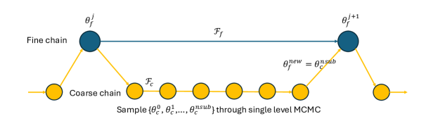
As can be seen from (27), the evaluation of the posterior requires the estimation of the first and second order moments of the output using GP samples. For each sample, the nonlocal meshfree method (21) is applied for each spatial point, time step, and observation, making this numerical evaluation expensive in MCMC. In order to improve the efficiency of the MCMC procedure, we employ the Multilevel Delayed Acceptance (MLDA) MCMC technique [64, 65], which exploits a hierarchy of models of increasing complexity to efficiently generate samples from an unnormalized target distribution. For the purpose of illustration, we summarize the key factors of two-level Delayed Acceptance (TLDA) MCMC here, while the method could be extended to a model hierarchy with arbitrarily many levels by recursion. For the vanilla Metropolis-Hastings (MH) algorithm which is a typical single level MCMC, consider sampling a trace from a target distribution , using a proposal distribution , and an initial state . MH accepts a new proposal given for with probability
otherwise it rejects and sets . In the context of Bayesian inference, the MH target distribution is the posterior distribution, i.e. . Unlike the vanilla MCMC which has only one model, in TLDA, a cheaper model is employed to reduce the computational cost. Fig.1 illustrates the work flow for TLDA, where the coarse subchains are sampled in order to provide proposals for the fine model. Denote by the fine forward model and by the coarse forward model, with and being their target distributions respectively. Starting from , in the coarse level, one can generate the subchain of length using MH or any single-level MCMC method. After the subchain is finished, we take as the proposal for the fine chain (i.e. ) and accept this proposal with probability
| (28) |
otherwise reject and set [65].
When the approximation provided by the coarse model is poor, many samples will be rejected by the fine model resulting in a very low acceptance rate. As outlined in [65], an enhanced Adaptive Error Model (AEM) based on [82] is useful to account for and correct the discrepancy between the fine and coarse models. We use the two-level AEM [82, 65] in the present use of TLDA. For parameters and operating conditions , the bias between the two models can be written as
| (29) |
When the parameter set is sampled from the prior distribution, then
Denoting the fine model solution as , the coarse model (the step-wise nonlocal model) solution as , and the trainable parameter set as , we have the following sample mean and standard deviation for the correction term
| (30) | ||||
where
| (31) | ||||
Here, is the number of samples of which will be used for computing the sample mean and standard deviation. We highlight that the enhanced model parameter set should be sampled simultaneously with . In contrast, and are calculated by averaging over multiple samples of only, for each fixed enhanced parameter set in (24). In other words, the sample moments computed in (31) are to be used for correction for any parameter inside the prior distribution instead of a fixed parameter.
By using the AEM technique, (27) can be well approximated by the coarse model following
| (32) | ||||
where and are the sample mean and variance for the correction term computed using (31). Technically, this step is also a reference for tuning the upper and lower bounds for the prior distribution of . Such an interval should be selected in such a way that at least at the log-negative posterior in (32) which is approximated by the coarse model and the AEM could roughly reproduce the log-negative posterior in (27) which is generated using the fine model. We summarize our method in Algorithm 1.
| (33) |
| (34) |
| (35) | ||||
| (36) |
4 Application: Homogenization for a Heterogeneous Elastic Bar
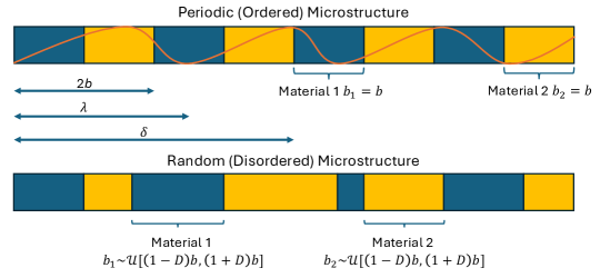
In this section, we examine the efficacy of the proposed ENOR approach on inferring the nonlocal homogenized surrogate for modeling the propagation of stress waves through a one-dimensional bar [22, 47]. In particular, we consider a composite bar either made of periodic layers or randomly generated layers (see Fig.2), and we assume that the amplitude of the waves is sufficiently small, so that a linear elasticity model is a valid way to describe the wave motion within the layers and at their interfaces. With this assumption of linear elastodynamics, the propagation of waves through the bar can be described as:
| (37) |
where is the mass density which is assumed to be constant throughout the body, is the displacement, and is the external load density. is the elastic modulus which varies spatially according to the microstructure, i.e., we have in the blue regions of Fig.2, and in the yellow regions. is the stress. On the interfaces of two materials, the following jump conditions hold: , .
Ideally, one can solve (37) using numerical solvers on fine discretizations of the computational domain to explicitly represent all interfaces. However, in real-world applications such as projectile impact modeling [21, 83], one is interested in modeling the decay of the wave over distances that are several thousand times larger than the layer size. In these circumstances, a fine numerical solver is prohibitively expensive and a homogenized surrogate model is desired to provide scalable predictions.
In this example, we first generate short-term high-fidelity simulation data by solving (37) using characteristic line method. This method, which we denote as the direct numerical simulation (DNS) technique, assumes that the waves running in the opposite direction converge on the node, and update the material velocity explicitly from the jumping condition which is a consequence of the momentum conservation. Due to this property, this DNS solver is free of truncation error and approximation error as in the classical PDE solver, which allow us to simulate the exact velocity of wave propagation through arbitrarily many microstructural interfaces. We refer the reader to [21, 47] for more details of this method for further details. Then, our goal is to construct a nonlocal homogenized surrogate model from this high-fidelity simulation dataset .
4.1 Example 1: Periodic Microstructure
Throughout the section, a non-dimensionalized setting is employed for the physical quantities for the simplicity of numerical experiments, following the setup in [21]. First, we consider a periodic heterogeneous bar, where the layer size for the two materials is a constant . The bar length is and the physical domain is set to be . Components 1 and 2 have the same density and Young’s moduli are set as and , respectively. For the purpose of training and validation, three types of datasets/settings are considered:
Setting 1: Oscillating source (20 loading instances). We set . The bar starts from rest such that , and an oscillating loading is applied with with . Here we take .
Setting 2: Plane wave with ramp (11 loading instances). We also set the domain parameter as . The bar starts from rest () and is subject to zero loading (). For the velocity on the left end of the bar, we prescribe
for .
Setting 3: Wave packet (3 loading instances). We consider a longer bar with , with the bar starting from rest (), and is subject to zero loading (). The velocity on the left end of the bar is prescribed as with , , and .
For all data types, the parameters for the nonlocal solver and the optimization algorithm are set to , , , and . For training purposes, we generate data of types 1 and 2 till . Then, to investigate the performance of our surrogate model in long-term prediction tasks we simulate till for setting 3.
4.1.1 Results from MCMC Experiments
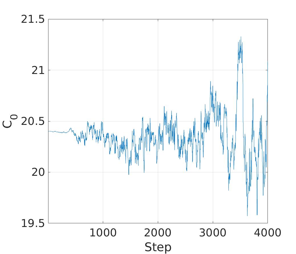
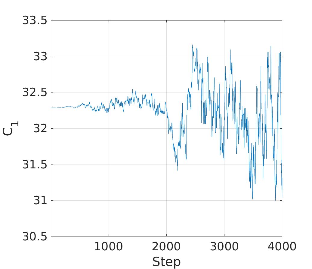
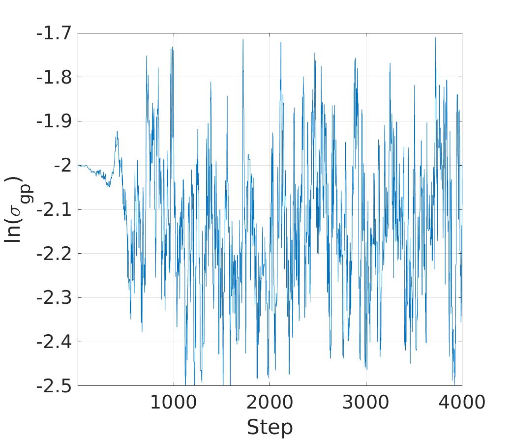
We use PyMC [84] for all the MCMC computations below. We begin by verifying the convergence behavior of our algorithm. In particular, we test a single-level MCMC with the differential evolution Metropolis (DEMetropolis) algorithm [85] on the fine level with 4,000 draws and a burn-in stage of 300. DEMetropolis, or DEMetropolis(Z) is a variation of Metropolis-Hastings algorithm that uses randomly selected draws from the past to make more educated jumps. Results in Fig. 3 indicate that the single-level MCMC suffers from an extremely long burn-in stage and poor mixing. We treat these single-level results as a baseline which we use to examine the relative performance of the multilevel method below.
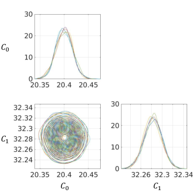
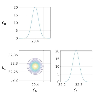
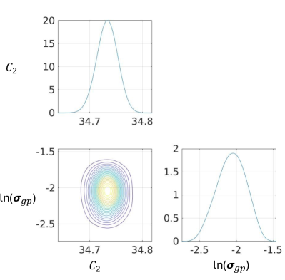
We first illustrate the utility of the multilevel algorithm using a correlation length . We run 6 independent chains, each with 4,000 draws, a burn-in stage of 300 and a subchain length on the coarse level of 100. Each chain is initialized using the scheme proposed in Section 3. We examine the quality of the chains both visually and quantitatively. Fig.4 illustrates that all the three independent chains attain essentially the same stationary state. Further, using the improved statistic [86] relying on ArviZ in Python, we find that the values for all 24 parameters are very close to 1, with the highest being , again highlighting the convergence of the chains. Note that, for an ergodic process, this statistic decays to 1 in the limit of infinite chain length [86].

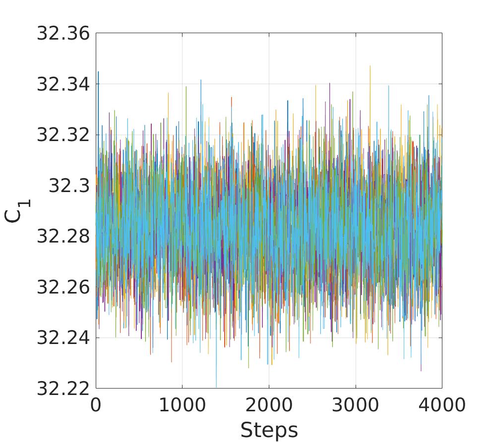
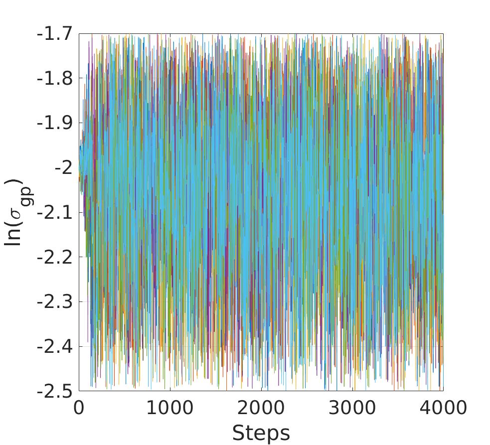
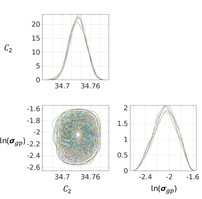
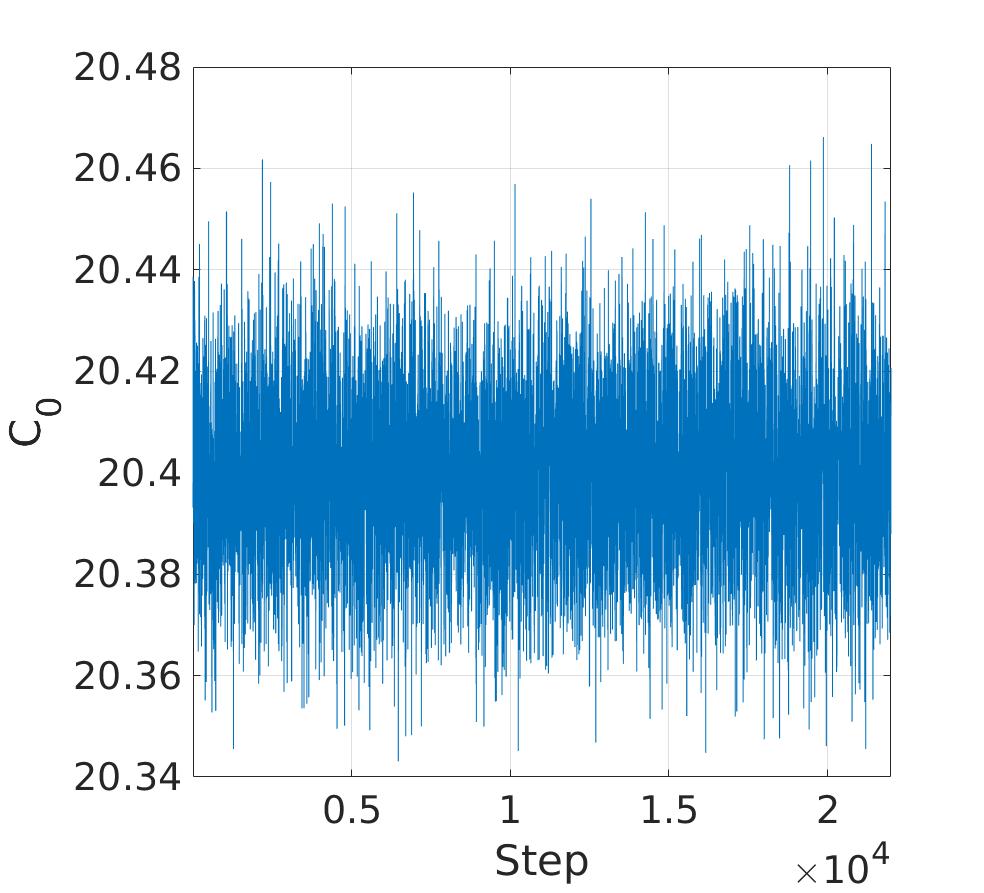
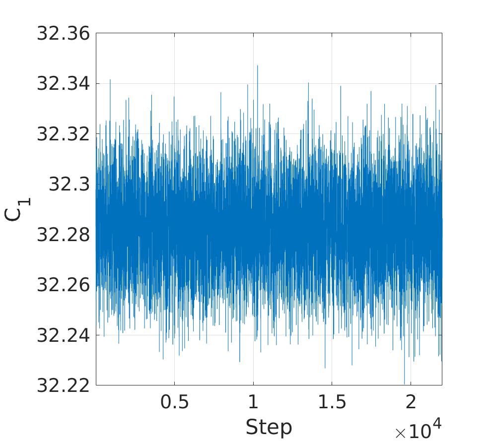
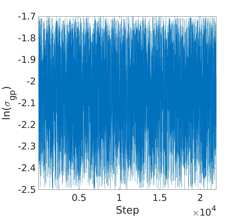
The chains have 24,000 draws in total, with approximately 42% acceptance rate on average. To present the aggregate results, we use roughly 6,000 equally spaced samples out of the total, where this effective sample size (ESS) was calculated using the method in [87]. The trace plots shown in Fig.5 indicate good mixing, and, with the high ESS, we have reliable probability density functions (PDFs) and associated statistics.
4.1.2 Impact of GP Correlation Lengths
As discussed in Section 3.1, to avoid the repeated cost of (18) and (19) at each MCMC step, we use the GP correlation length, , as a tunable hyperparameter. In this section, we investigate the impact of different values of on the learnt corrected kernels and the corresponding nonlocal solution behaviors.
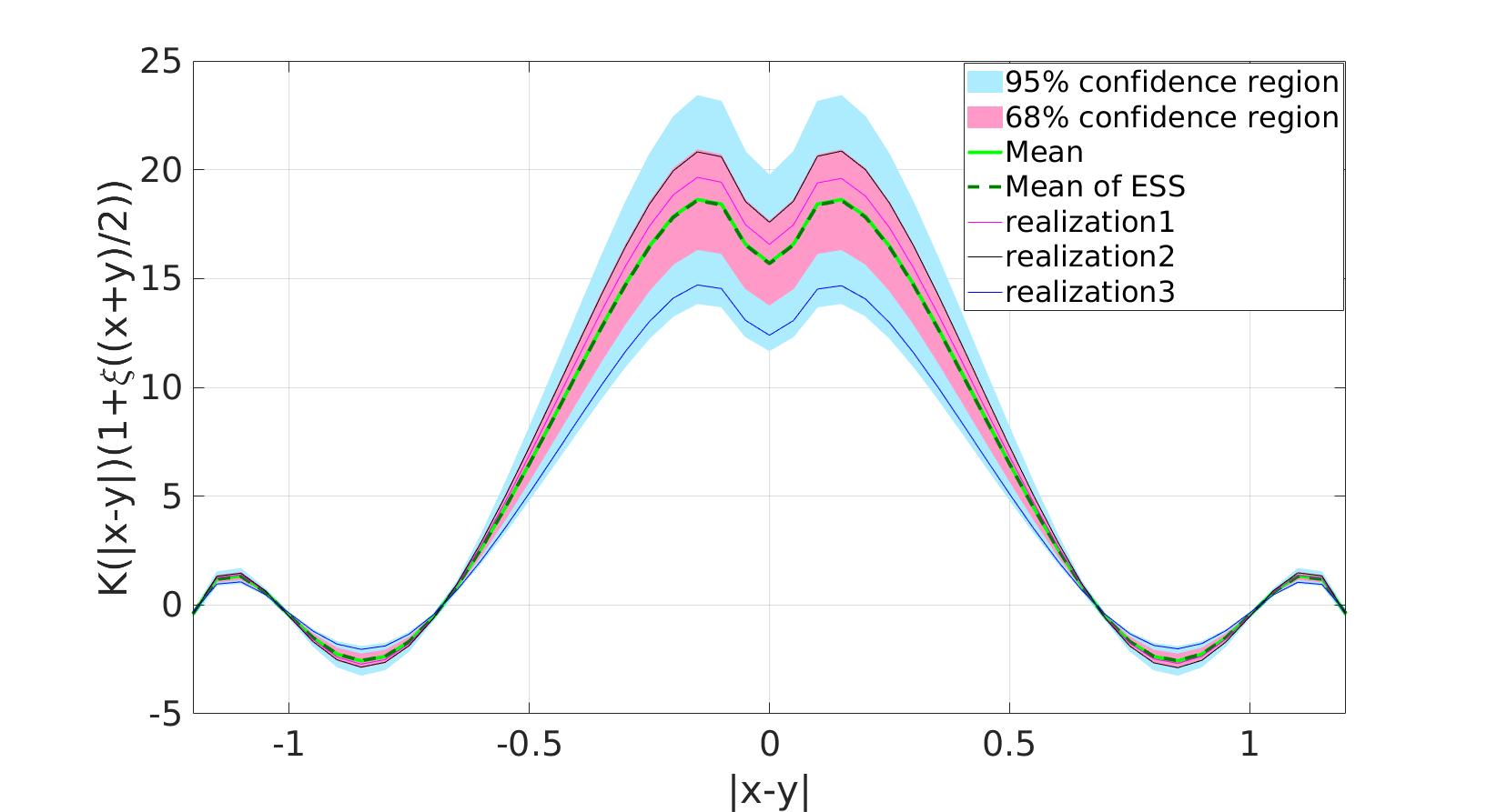
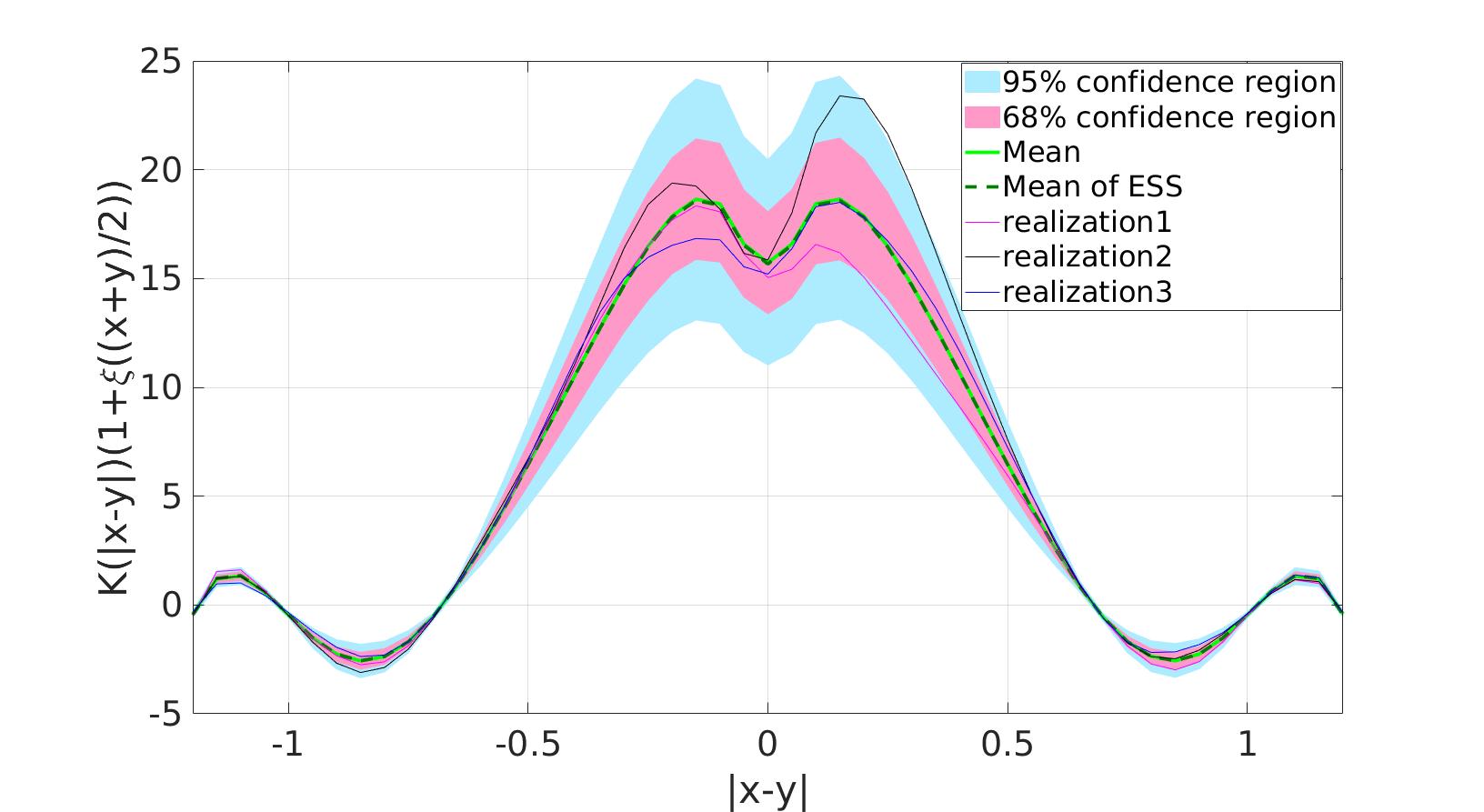
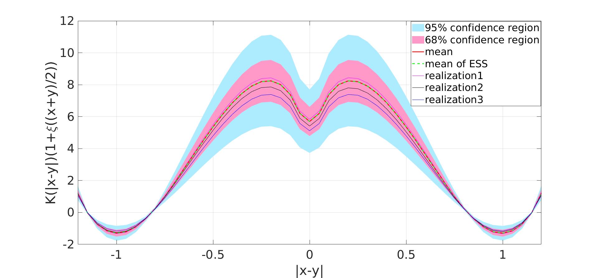
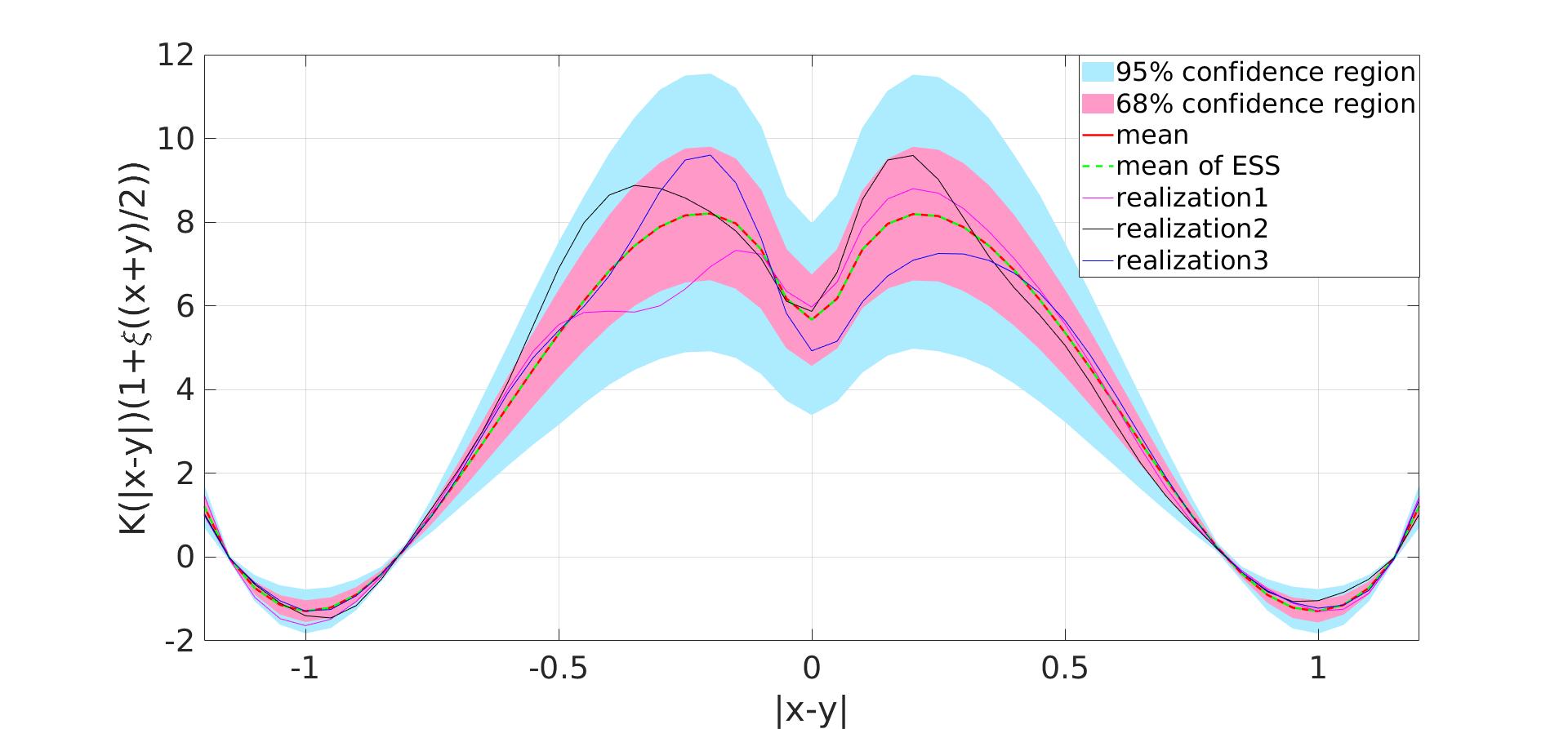
In Fig. 6, the uncertainty with several realizations for the kernel with GP, , is plotted for correlation lengths and , using 10,000 realizations in total. Since the behavior of the kernel is similar at each point in the one-dimensional bar, we pick the location as an instance for illustration. We observe that the curve labeled ‘Mean’, which is the mean value of all the realizations, is consistent with the corresponding kernel as the mean of the ESS, which is a single push-forward of the embedded model (16) using the mean value of the effective samples and setting the GP to 0. In fact, without the GP the embedded model degenerates to the original nonlocal model (2). This consistency is because of the linearity of the nonlocal kernel and the independence of the components. Further, for different values, one can barely see changes in the mean and the confidence region. On the other hand, sampled GP realizations exhibit significant structural differences between the two cases, in Figs. 6(a) and 6(b), consistent with the large change in between the two cases.
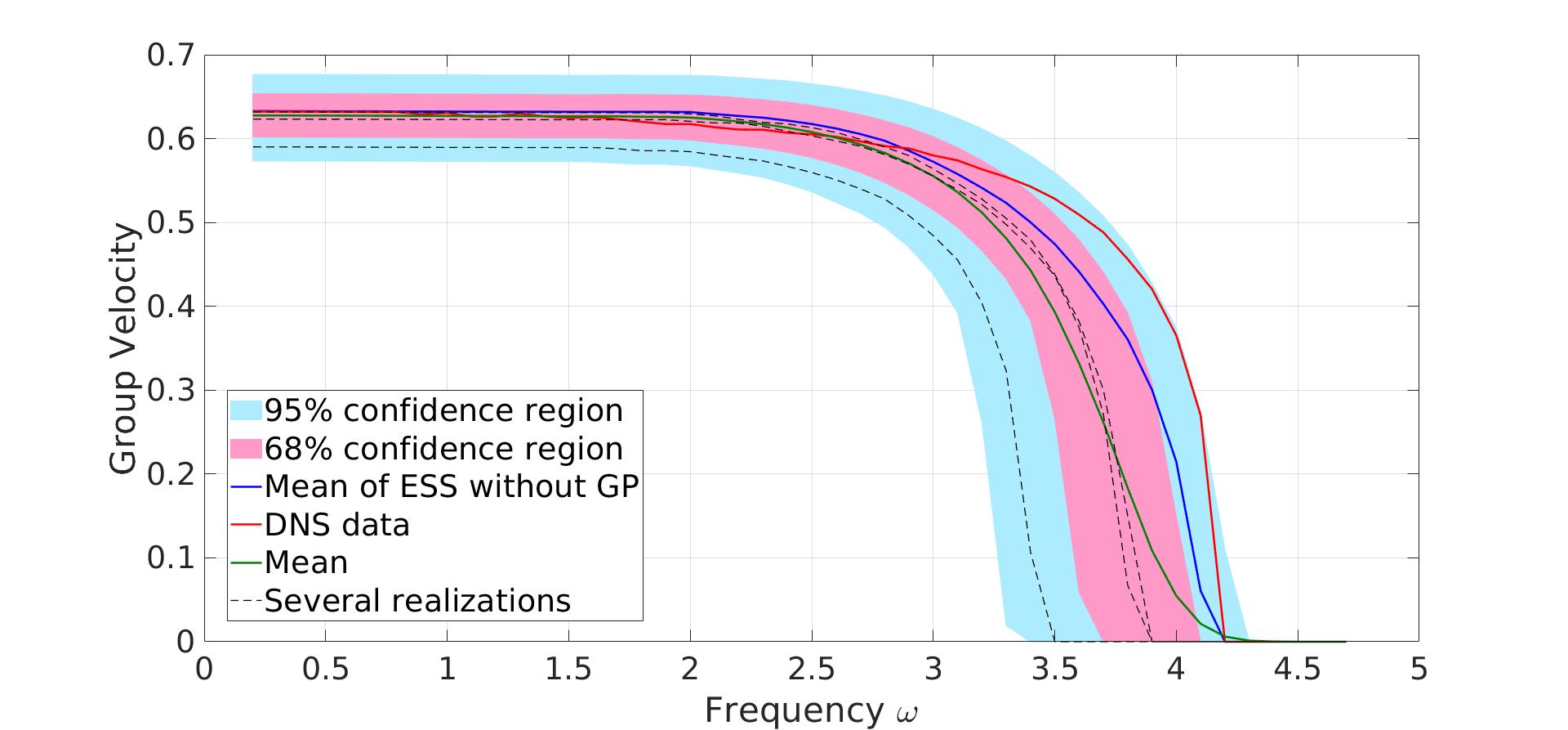
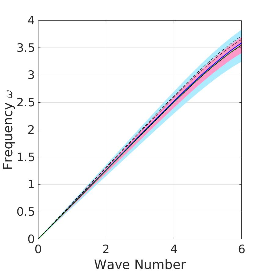
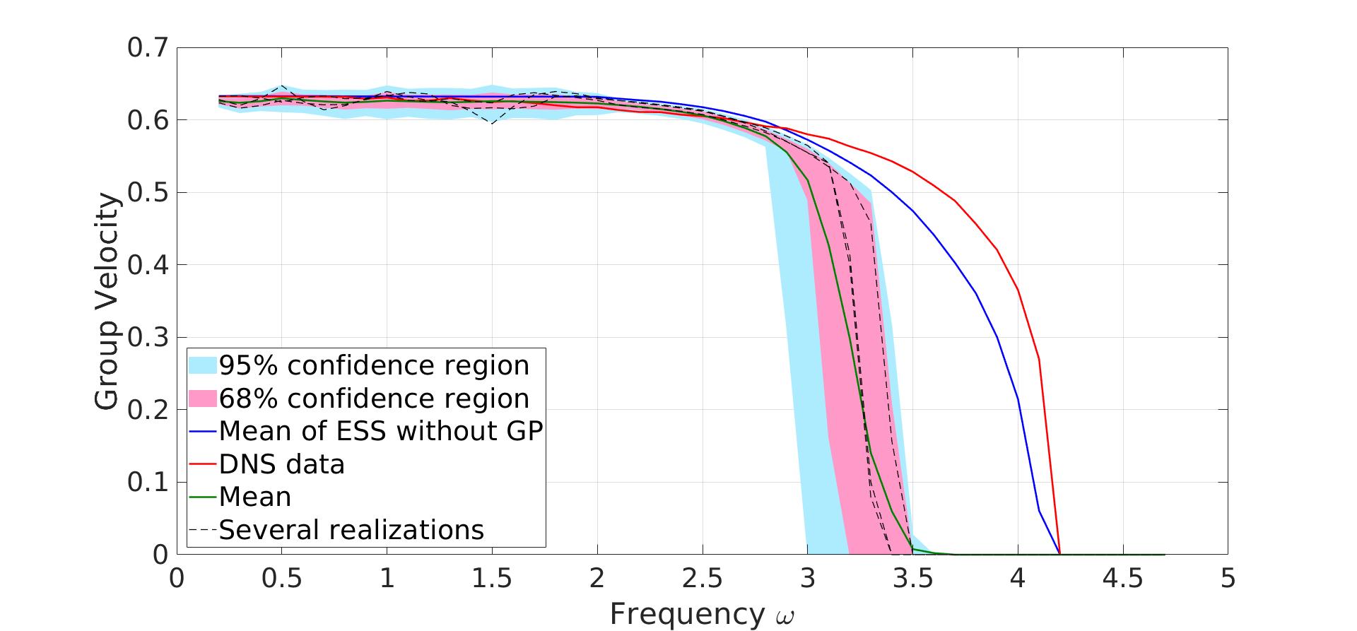
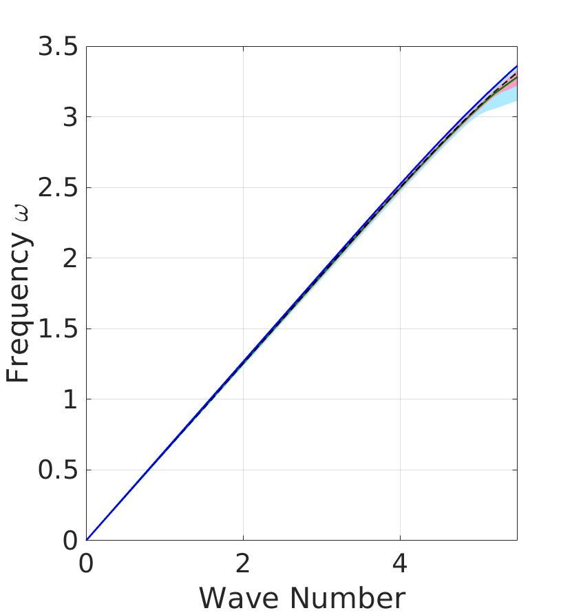
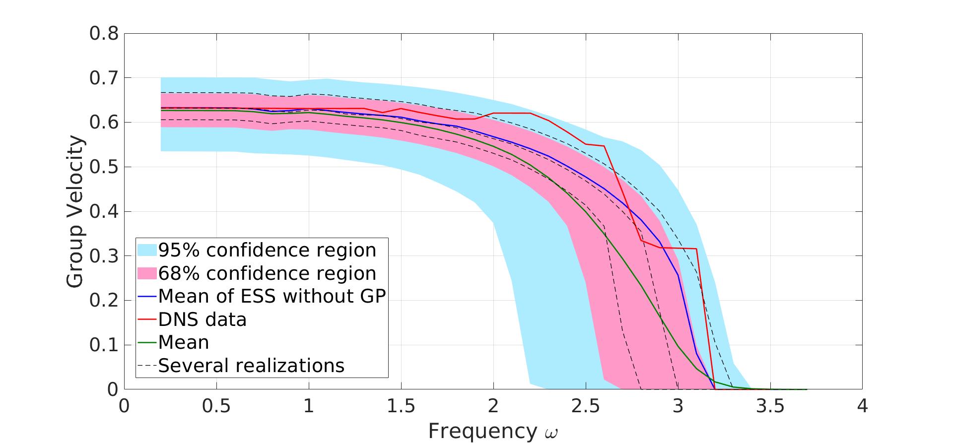
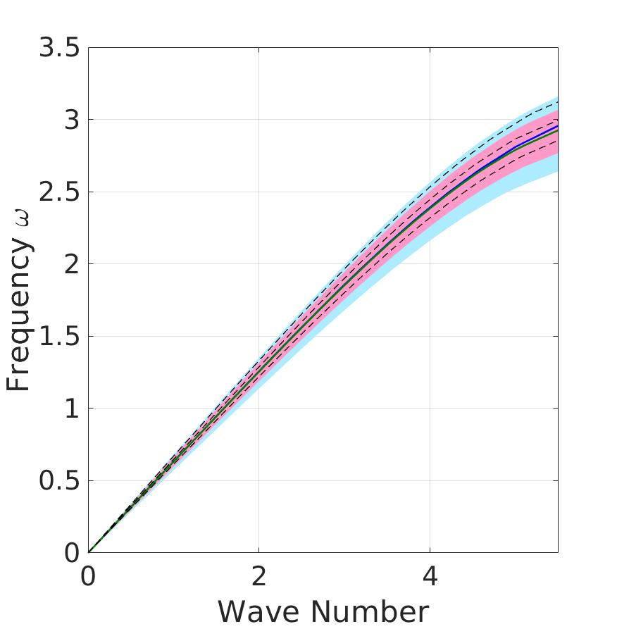
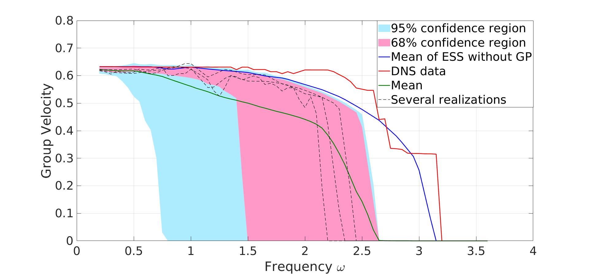
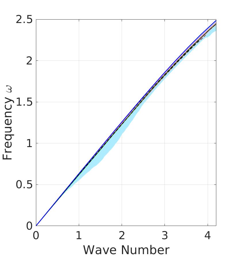
To examine the dispersion behavior of these kernel realizations, we plot in Figs. 7(a,c) the group velocity of kernels corresponding to a GP with a large () and relatively small () correlation length. For each realization of the kernel, the group velocity is computed using a wave packet that travels a long enough distance such that the wave is away from the ends of the bar. In order to do this in numerical simulation, we set the bar length equal to 400 and generate realizations of the kernels with the same correlation length on this longer bar. We note that the reduction in results in a reduced band stop location (the smallest frequency where the group velocity drops to zero). Further, it is evident that the confidence region matches the dispersion behavior better when using a large correlation length. At the same time, oscillation is observed in the low frequency () region in the small case. Finally, in Figs. 7(b,d), we plot the dispersion curves of these kernels. Note that all learnt kernels are positive, highlighting the physical stability of the corresponding nonlocal models.
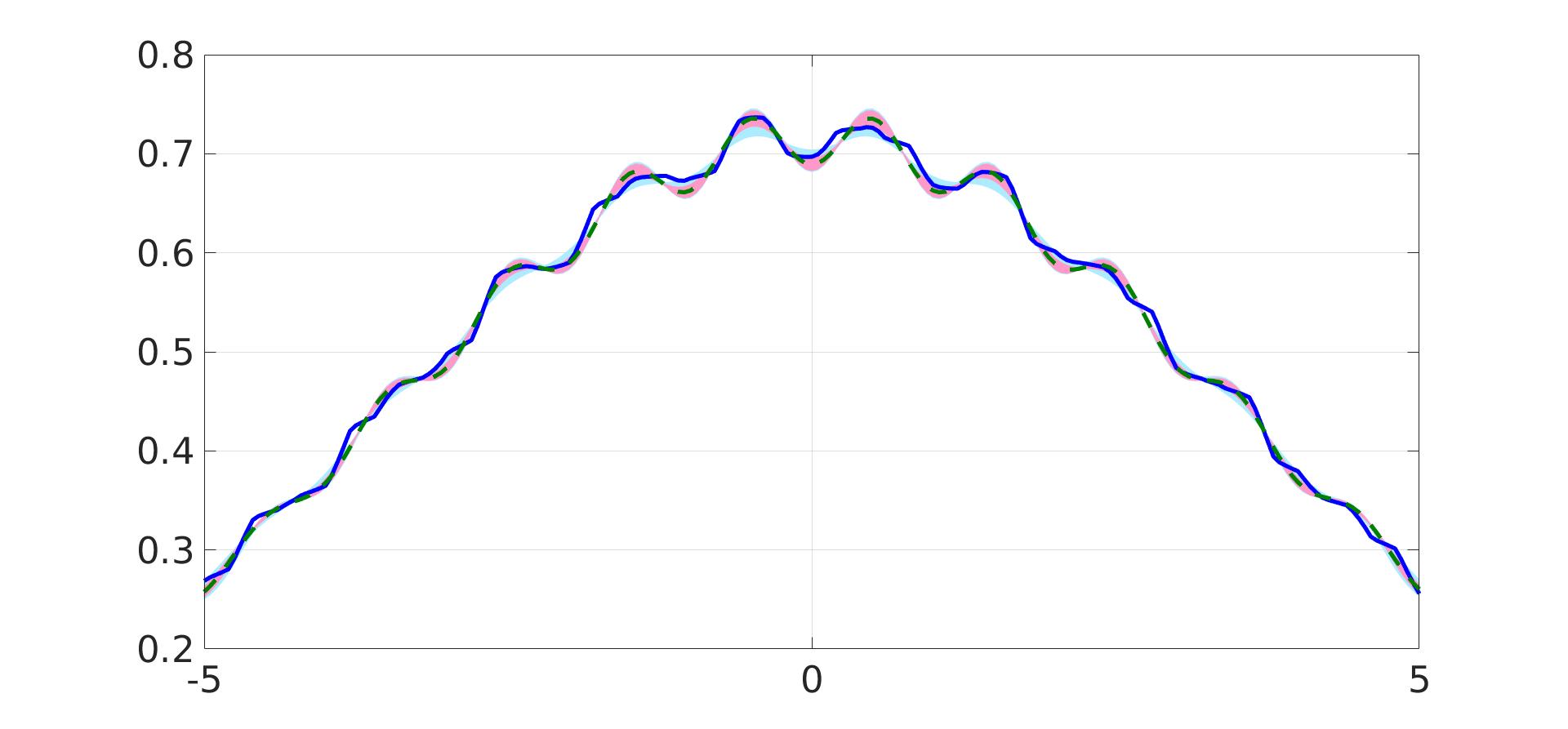
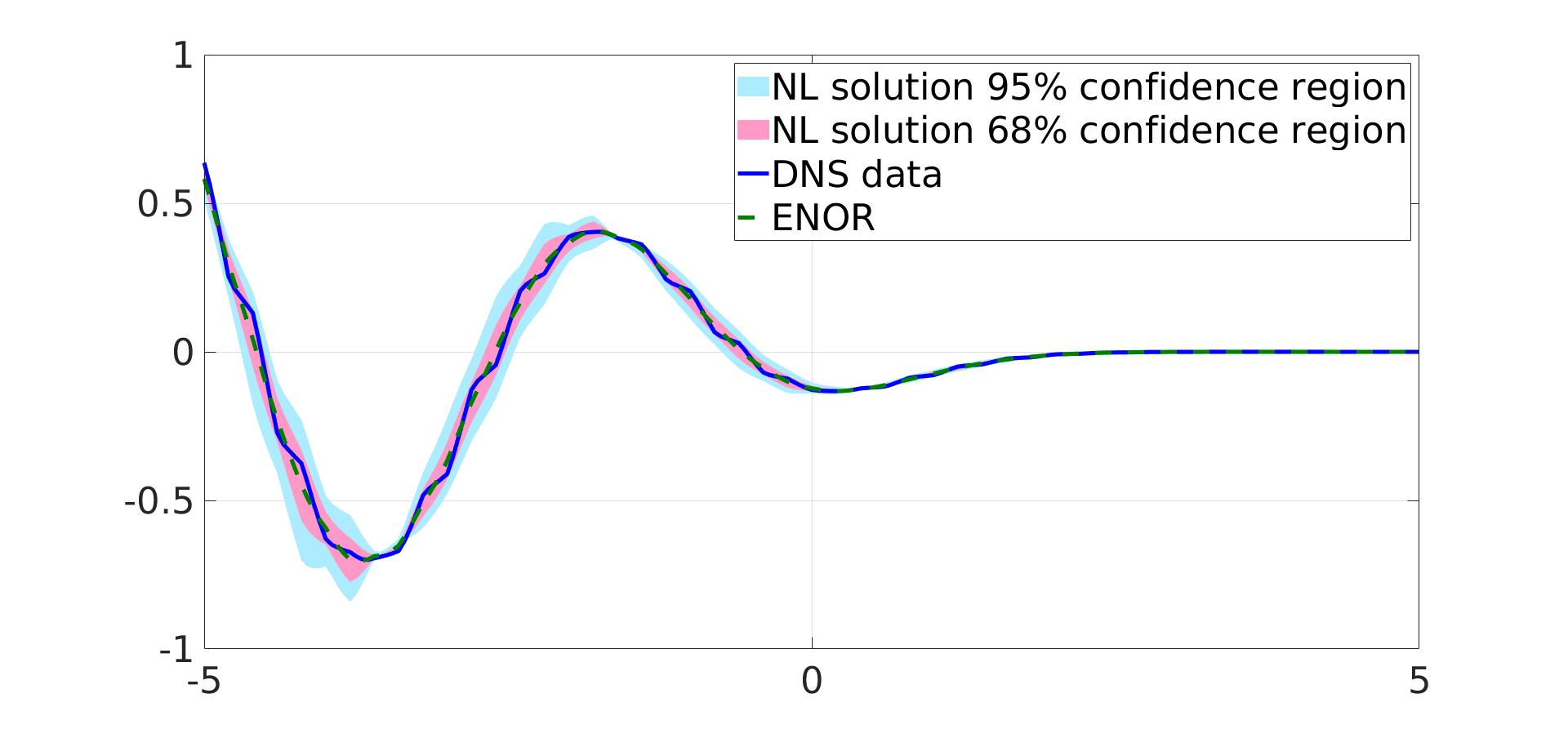
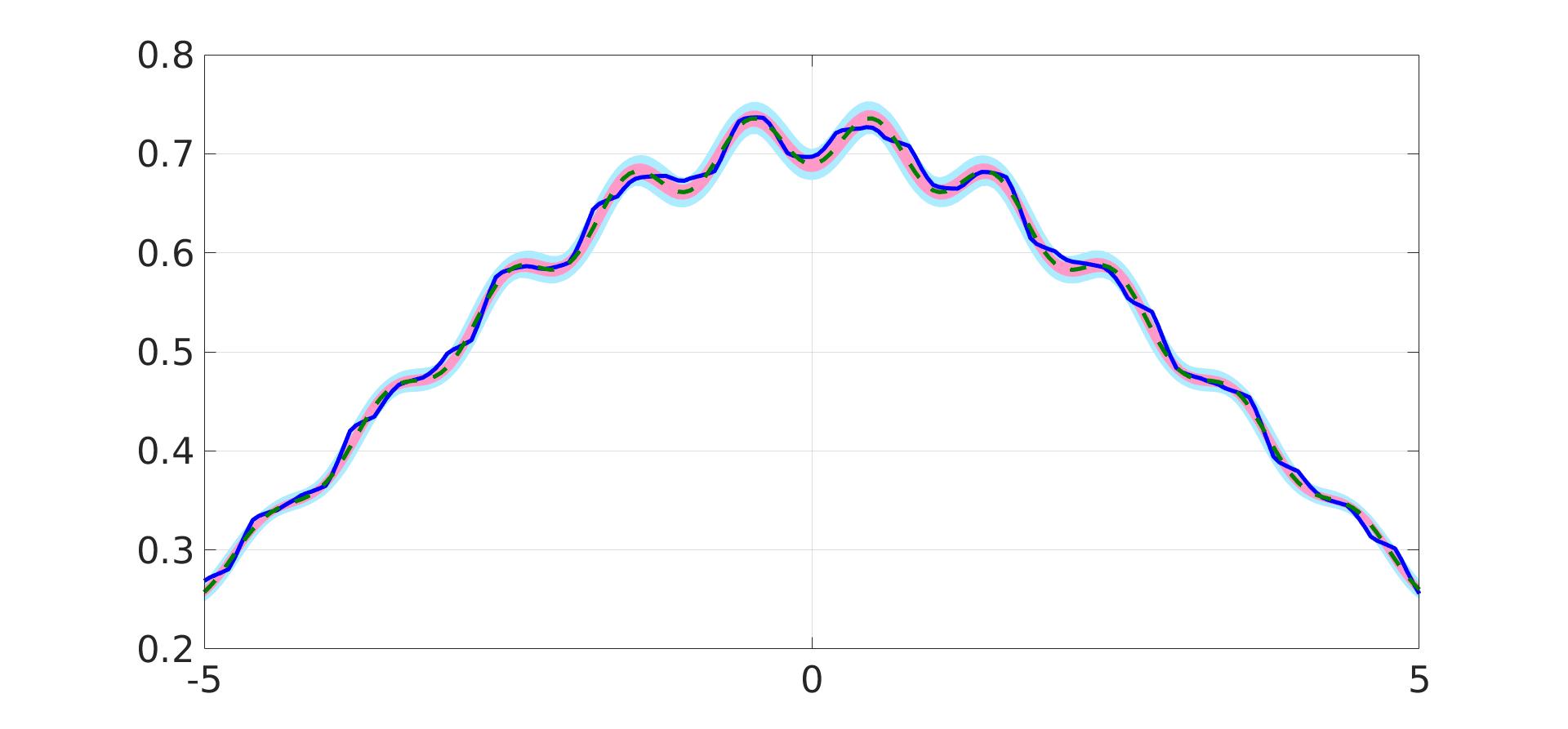
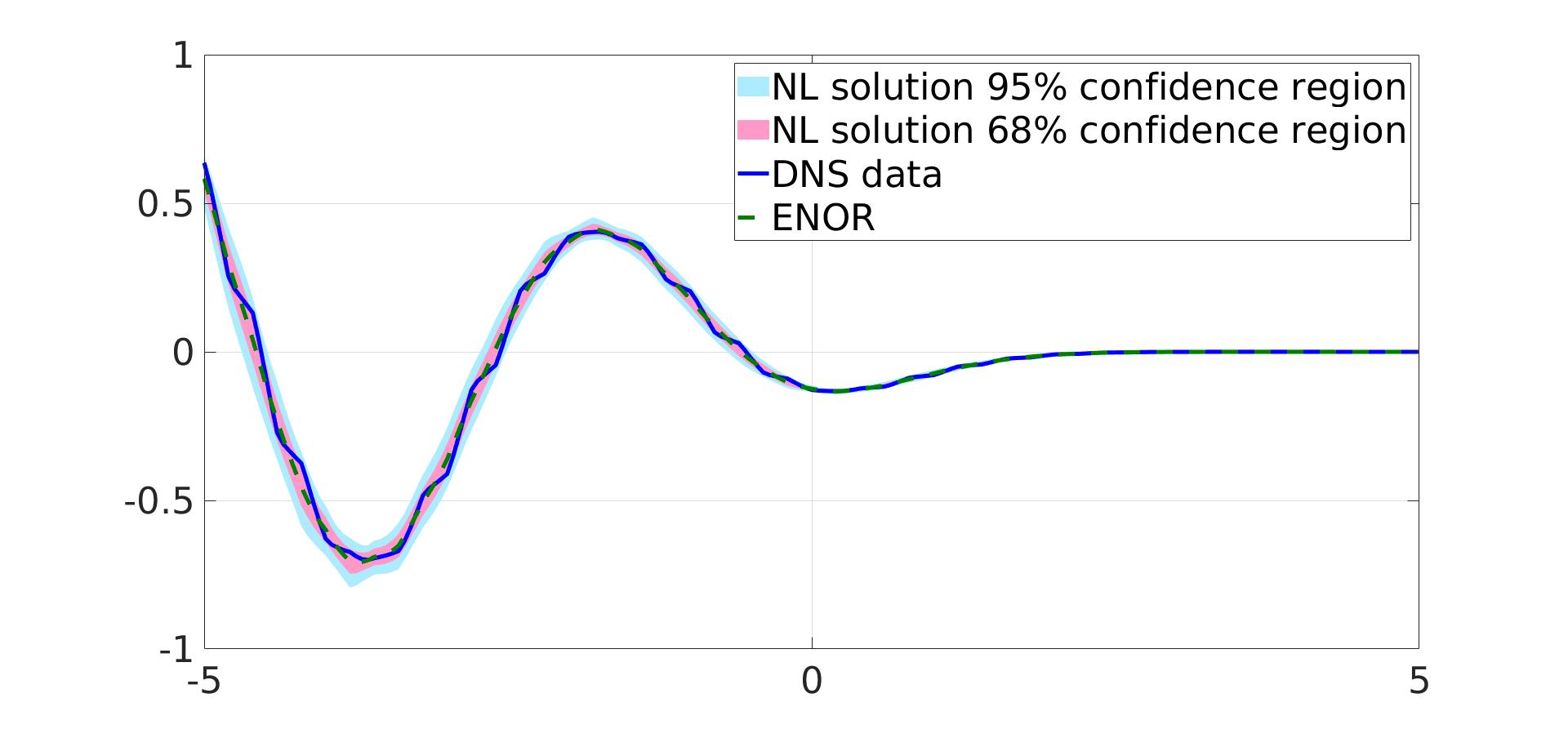
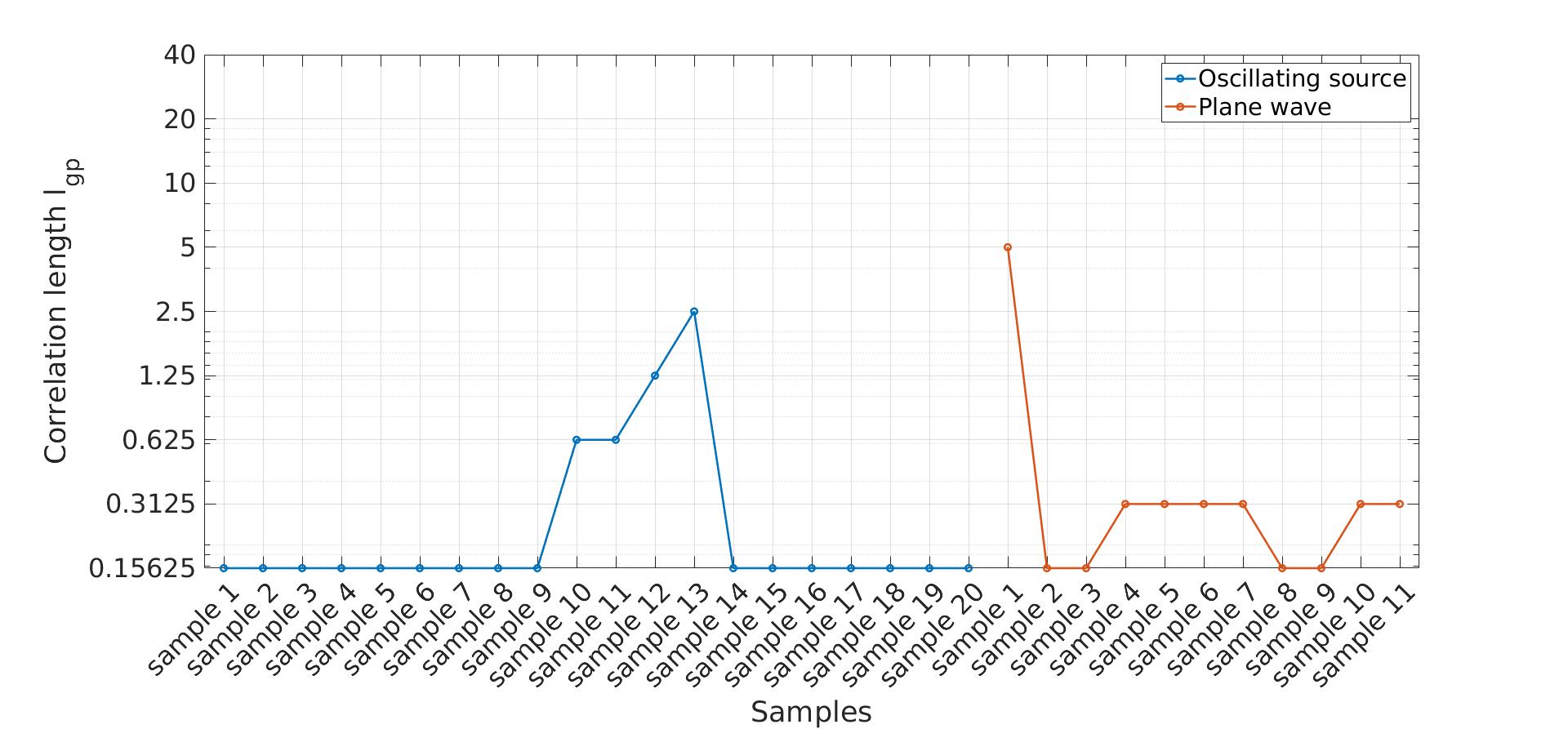
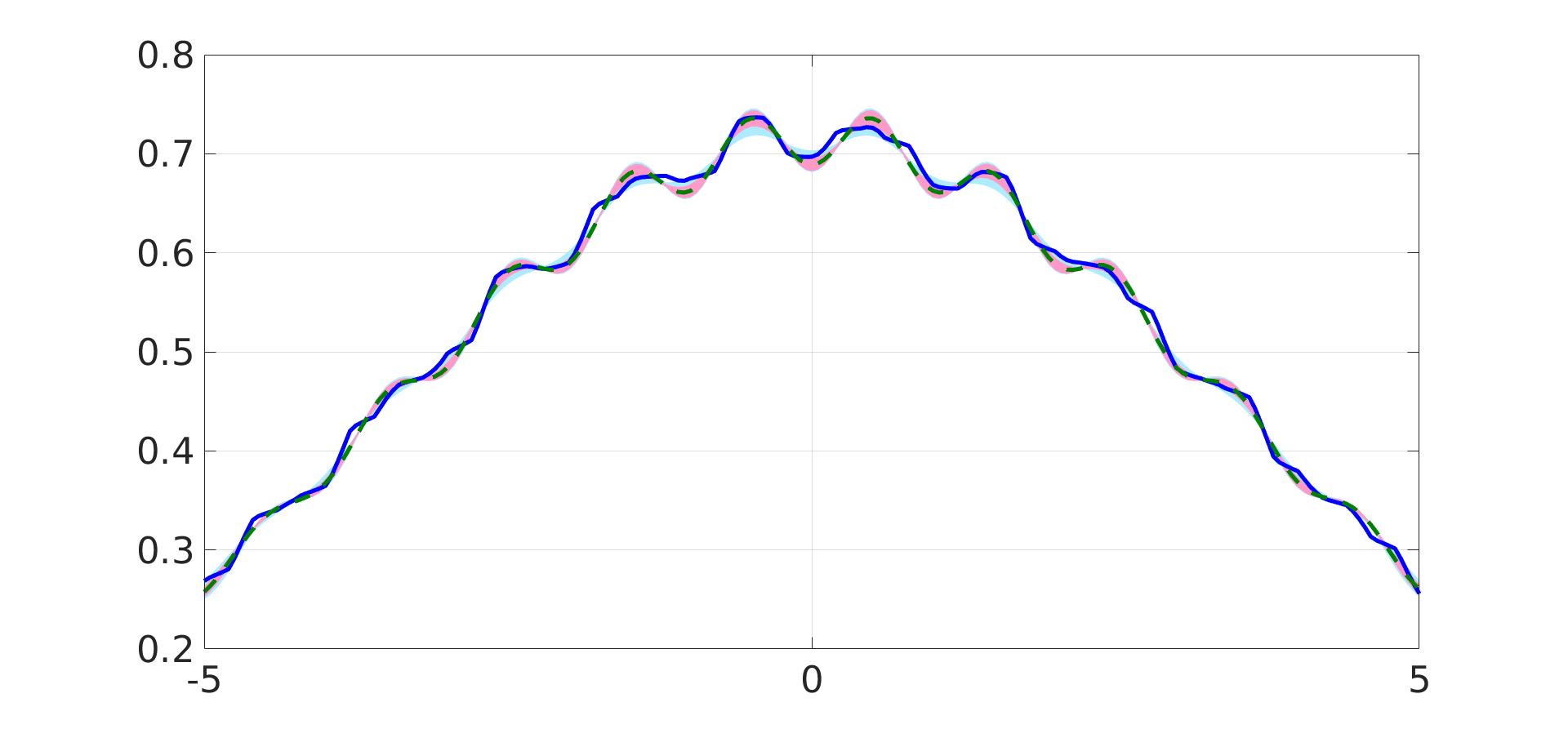
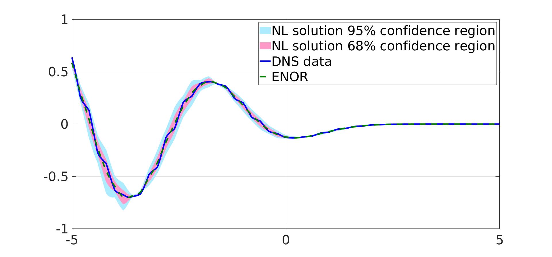
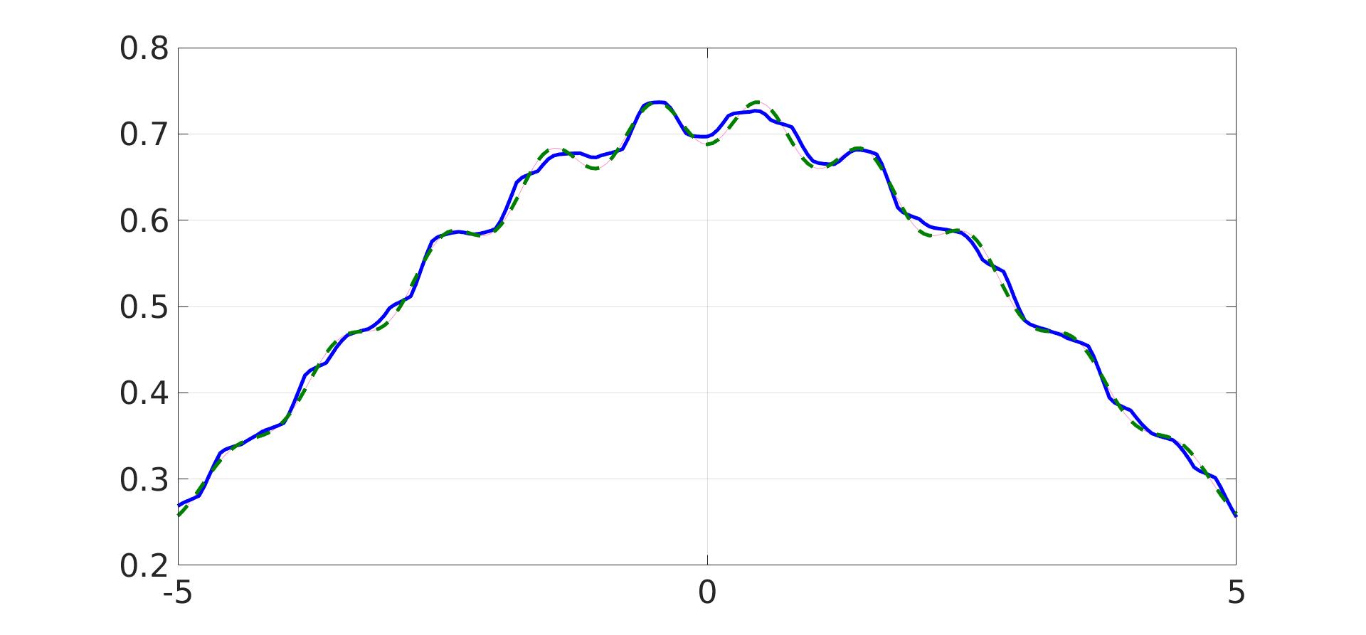
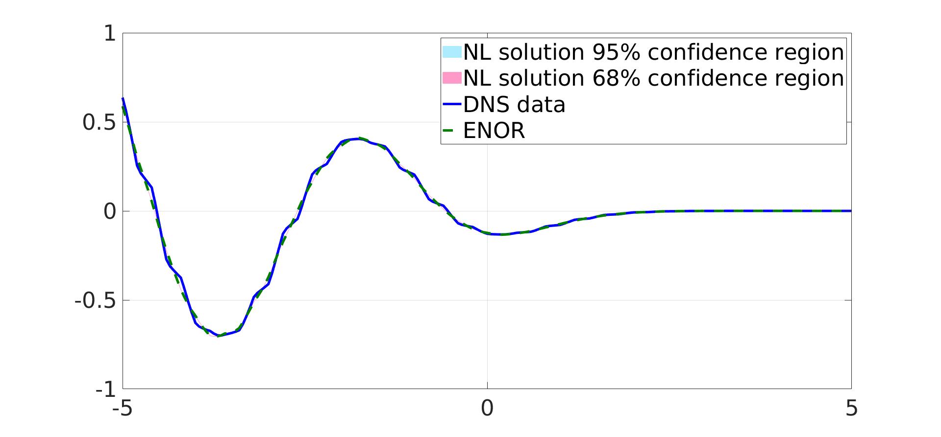
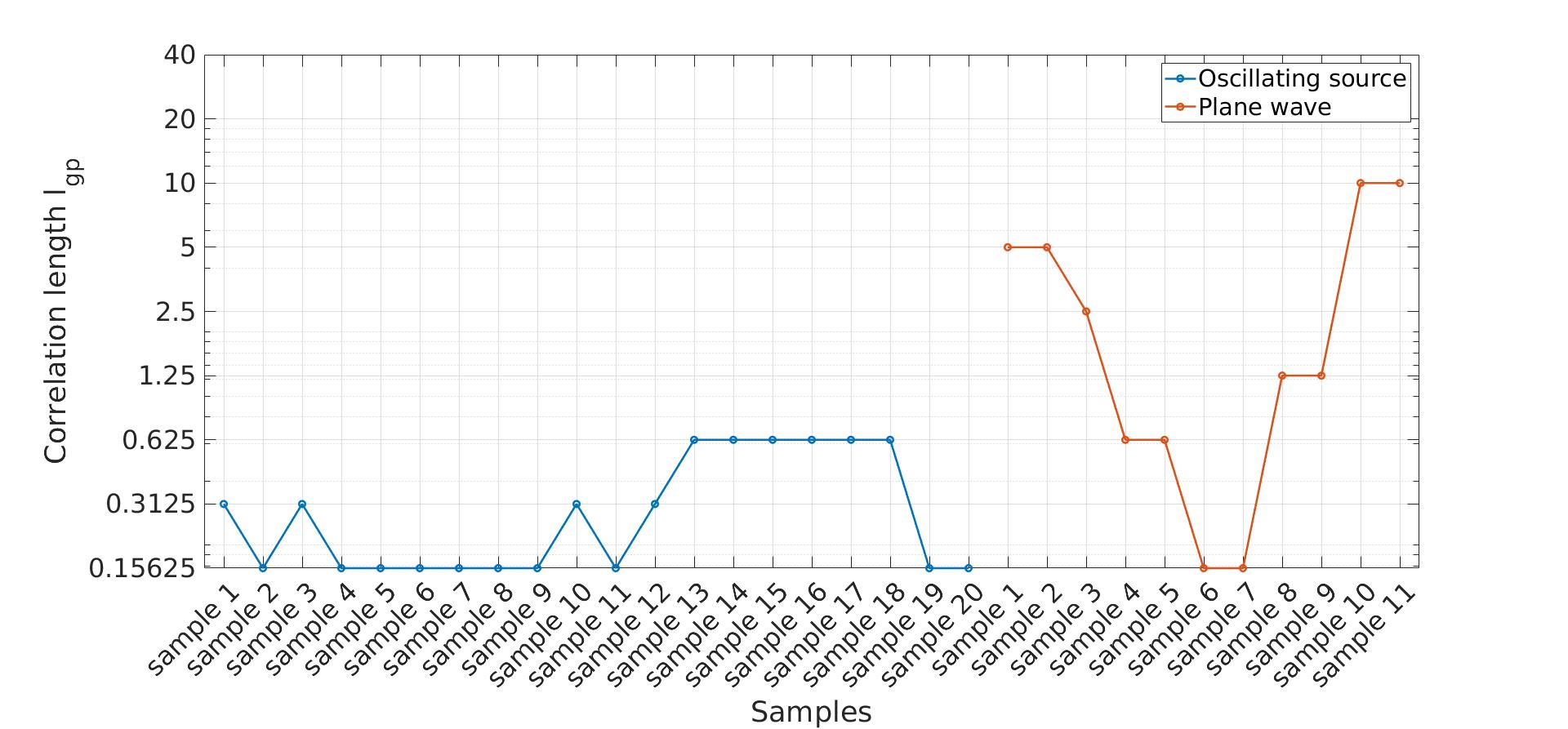
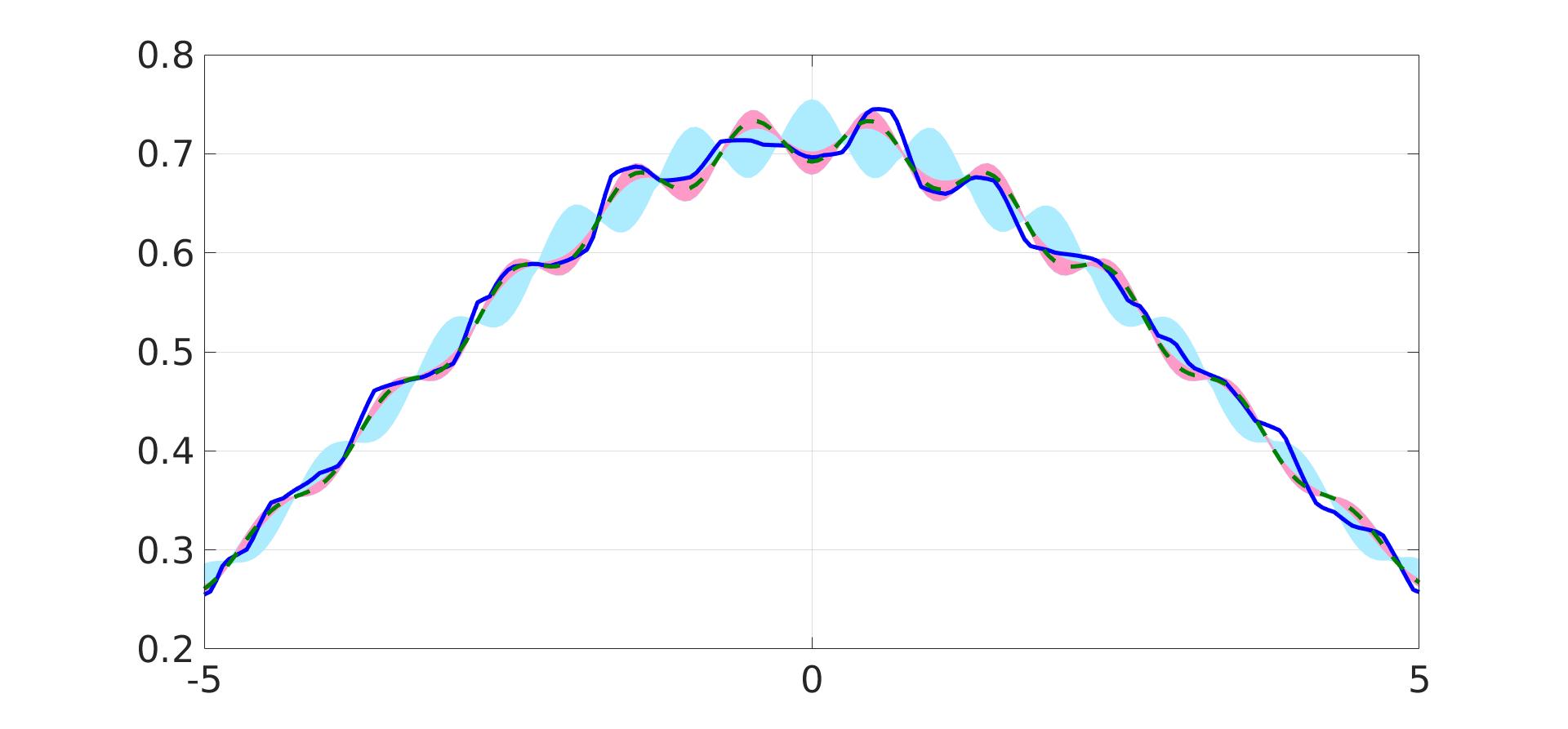
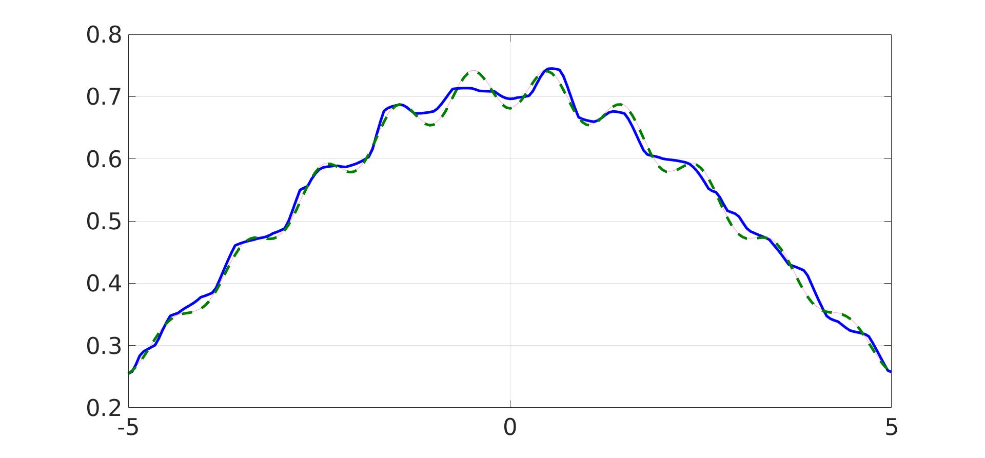
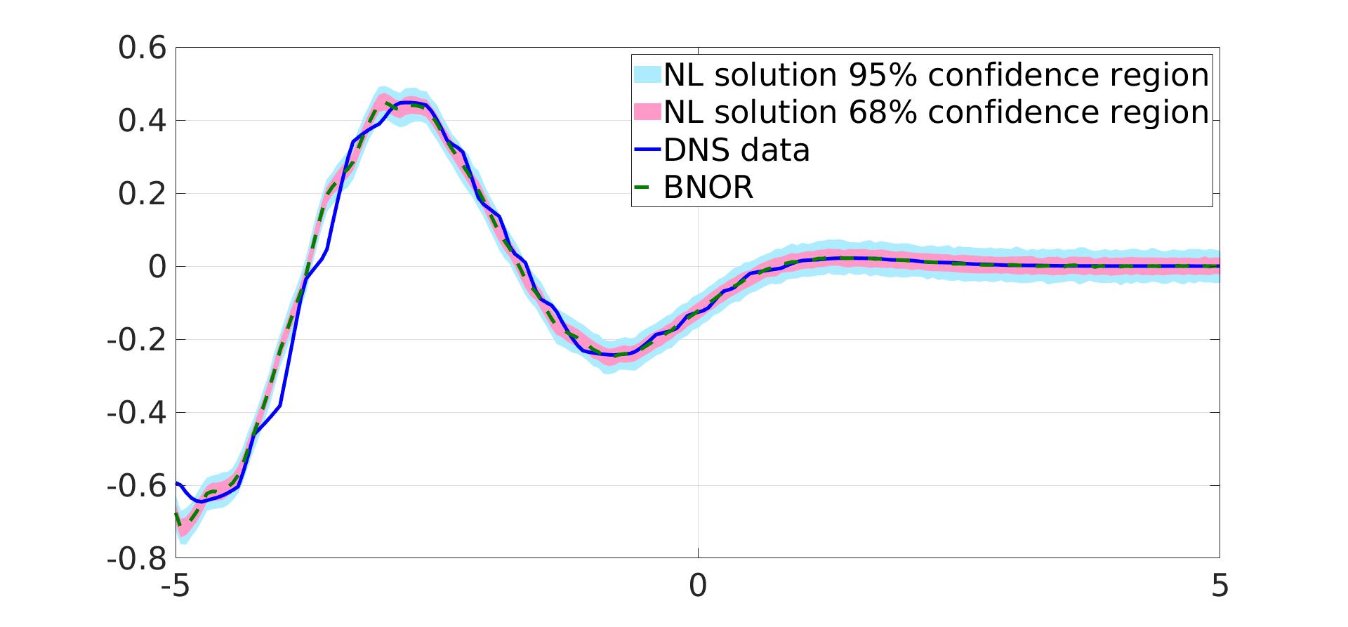
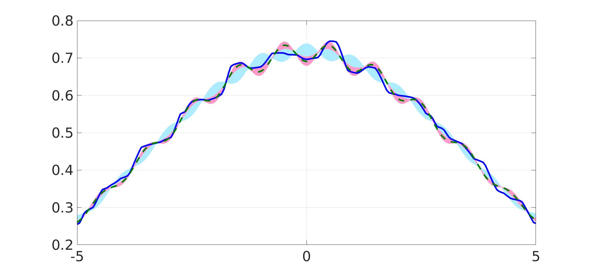
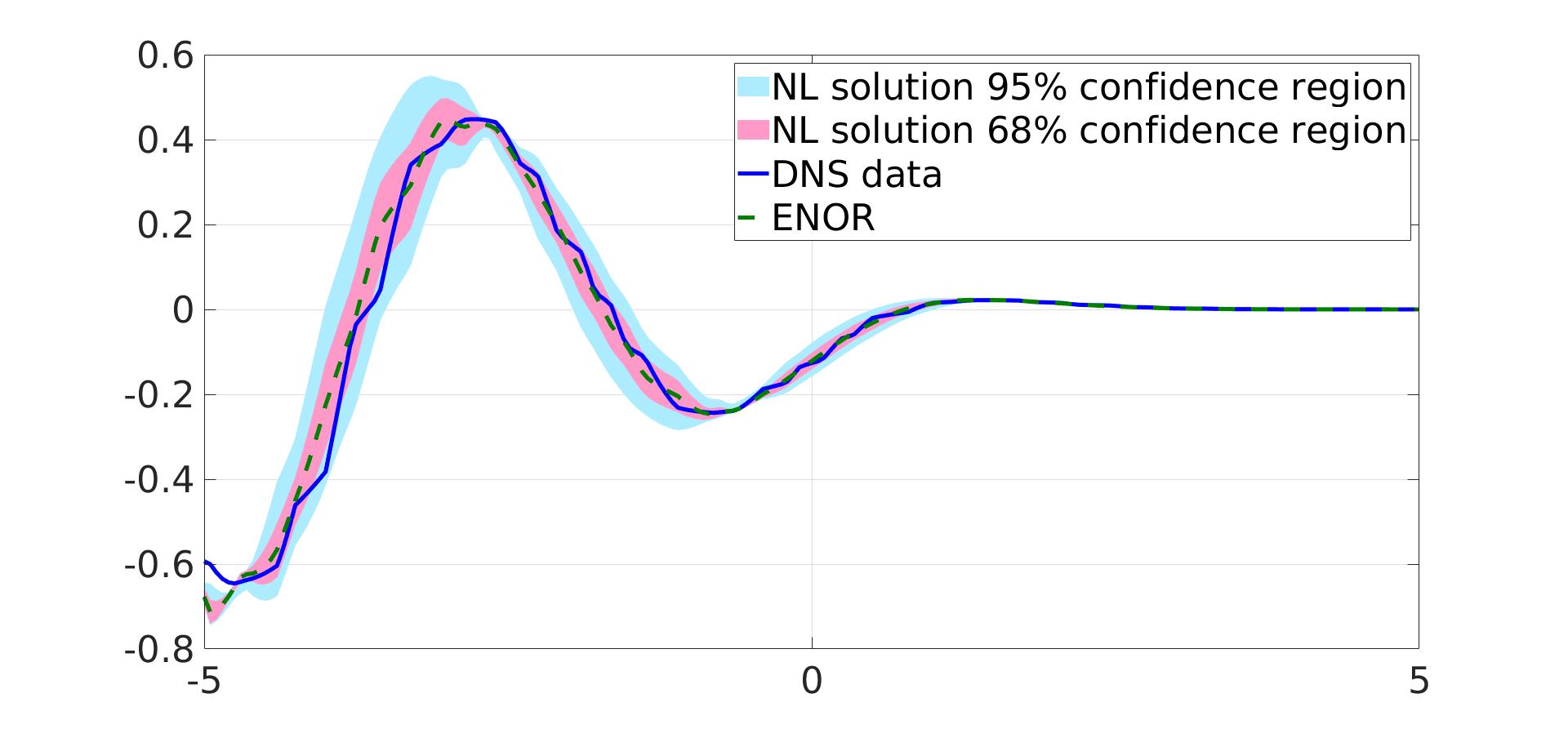
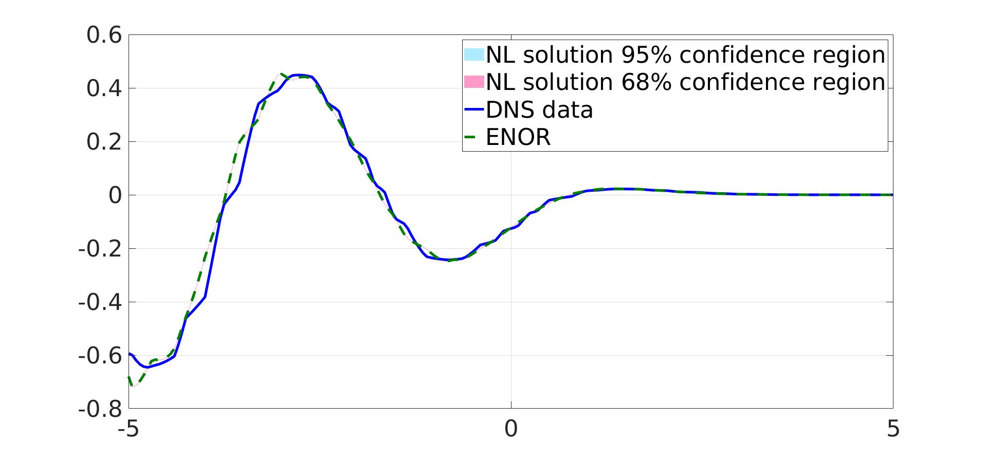
Next, we investigate the posterior uncertainty on the predicted displacements from the learnt models. Two samples from setting 1 and 2 datasets are considered, with forcing at in setting 1 and in setting 2. Let us first recall the definitions of two relevant push-forward posteriors for a typical additive data noise problem setup given the parameter posterior . We have the push-forward posterior (PFP) as the push-forward of the parameter posterior through the predictive model , while the posterior predictive (PP) is defined as the push-forward of the parameter posterior through the full data model [88, 89]. Note that, in an embedded model-error construction with no additive data noise, the PFP and PP are equivalent. In Fig.8, the PFP, which is the push-forward of the posterior through the nonlocal model with embedded model error, is plotted for two different values. For each case, we see that both the 95% and 68% PFP confidence regions generally cover the majority of the ground truth data over the spatial domain. However, we do observe that, visually, and for these two samples, the kernel with a smaller does a better job of spanning the ground truth data discrepancy from the mean model. This is also illustrated in Fig.10, where the best choices of for different training samples are plotted according to the Continuous Ranked Probability Score (CRPS) [90]. The CRPS compares a single ground truth value to a distribution. Assume that we have a ground truth and a cumulative distribution function (CDF) for a variable , then the CRPS can be analytically written as
In a numerical setting where only a sampling-based empirical CDF is available, [90] provides alternative forms of the CRPS which are feasible to estimate
| (38) | ||||
| (39) |
where , are independently and identically distributed according to . Per the definition of the CRPS, the lower the score is, the better does our predicted displacement match the DNS data in distribution. Specifically, we use equation (38) here, but in principle the two expressions are equivalent. The average CRPS values across different training samples, at , are summarized in Table.1. As the correlation length decreases, only a slight reduction in the CRPS is obtained, suggesting that all studied kernels have comparable performance in obtaining the correct distribution of the displacement.
| Material | |||||||||
|---|---|---|---|---|---|---|---|---|---|
| Periodic | 0.0048 | 0.0048 | 0.0048 | 0.0048 | 0.0047 | 0.0046 | 0.0045 | 0.0044 | 0.0043 |
| Disorder | 0.0080 | 0.0080 | 0.0080 | 0.0079 | 0.0079 | 0.0077 | 0.0076 | 0.0076 | 0.0076 |
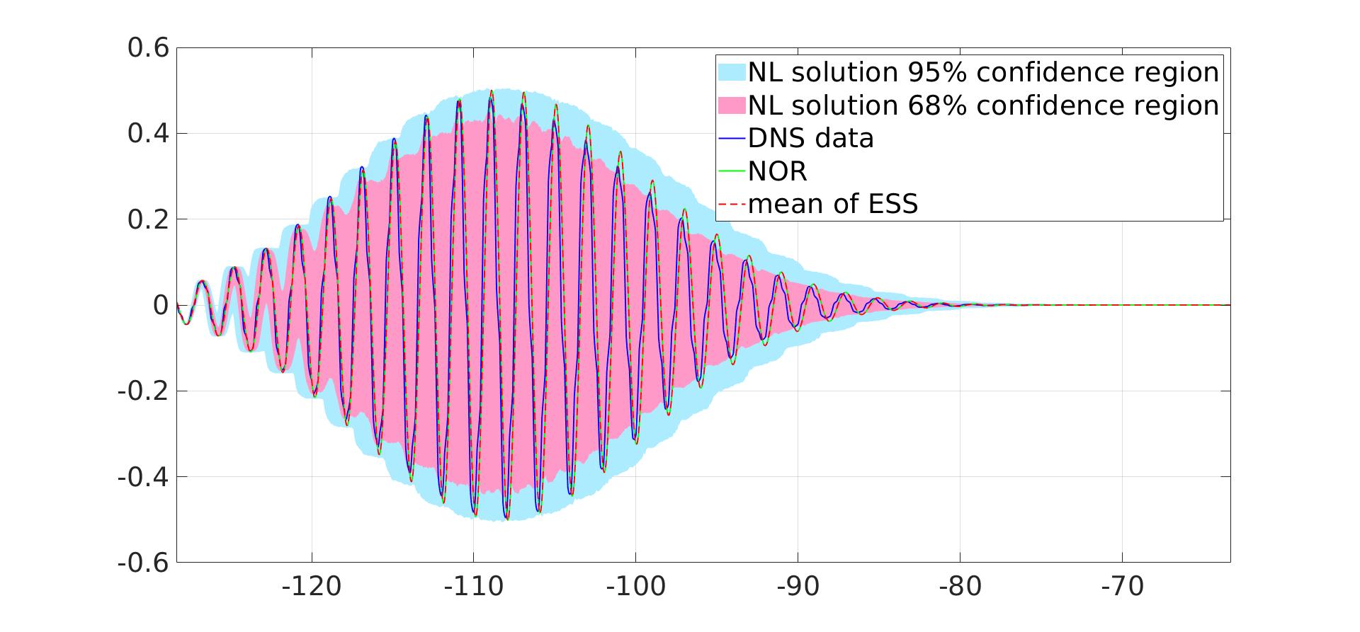
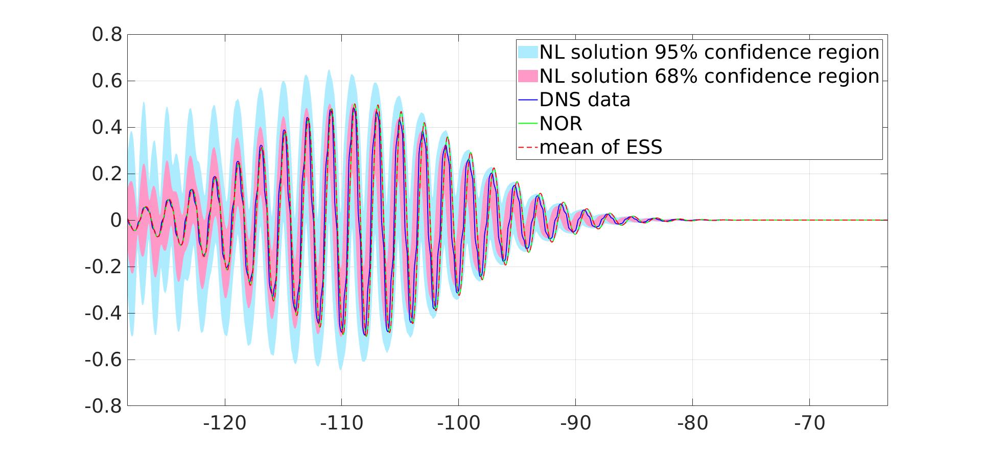
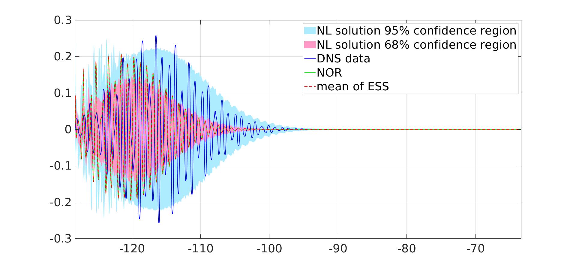
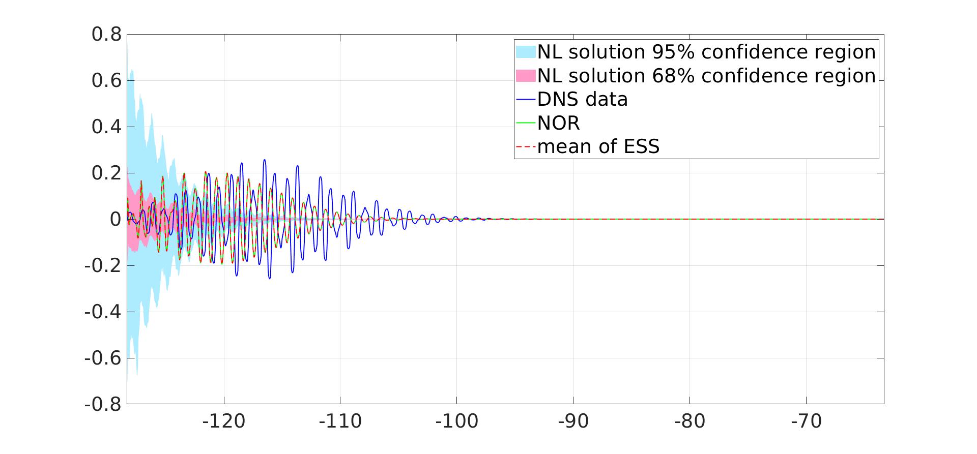
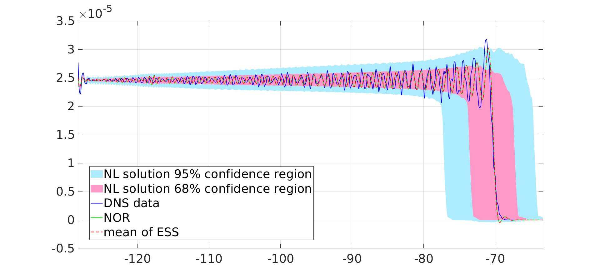
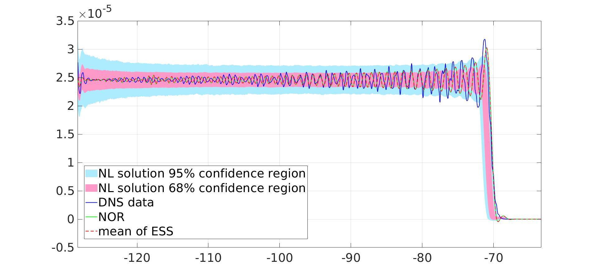
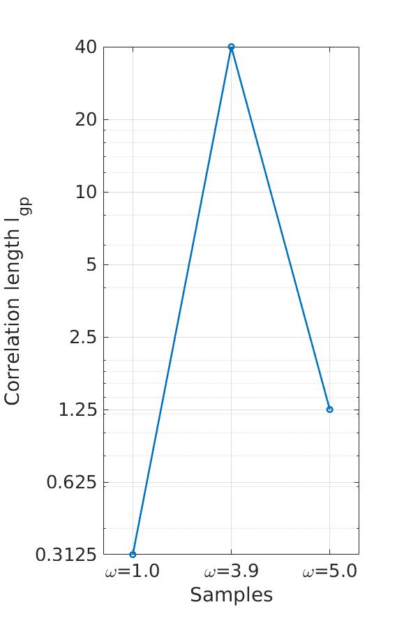
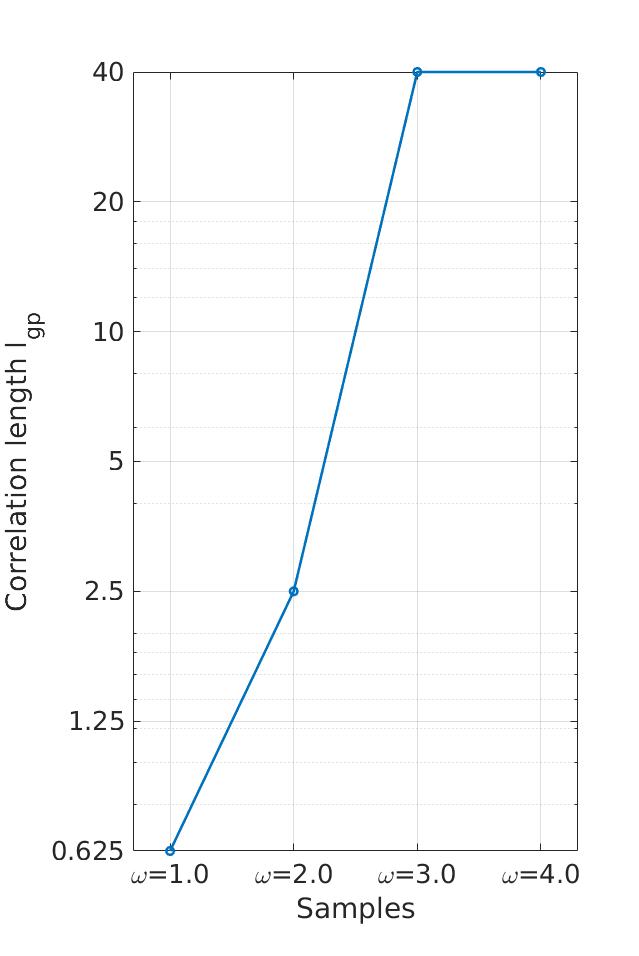
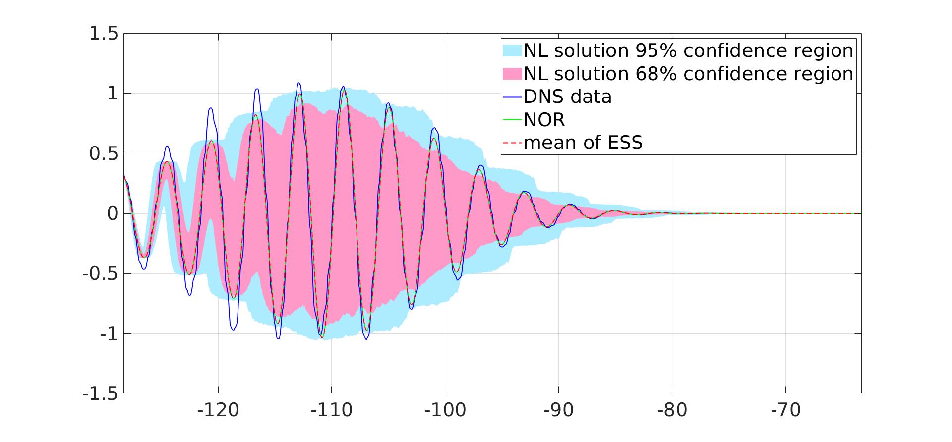
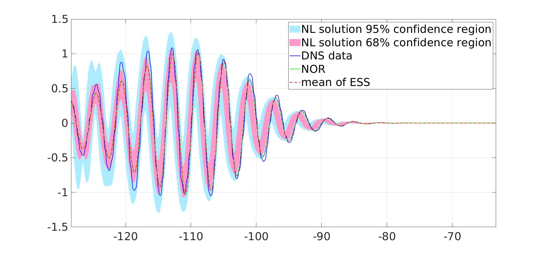
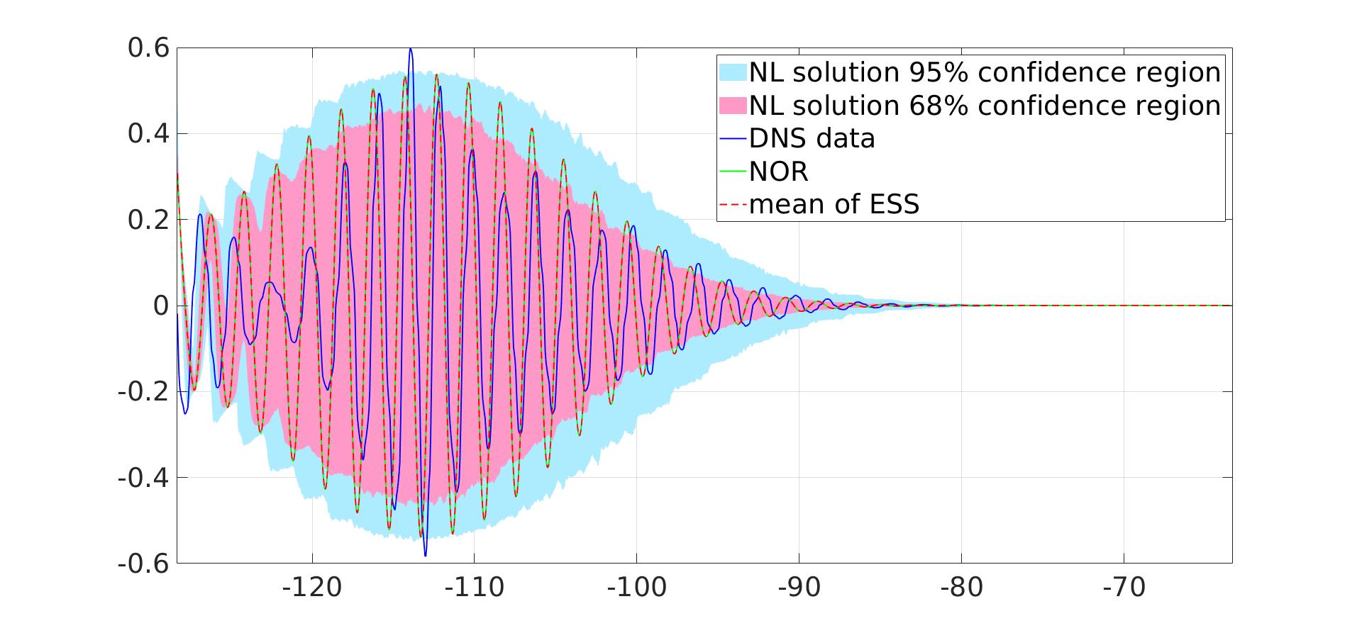
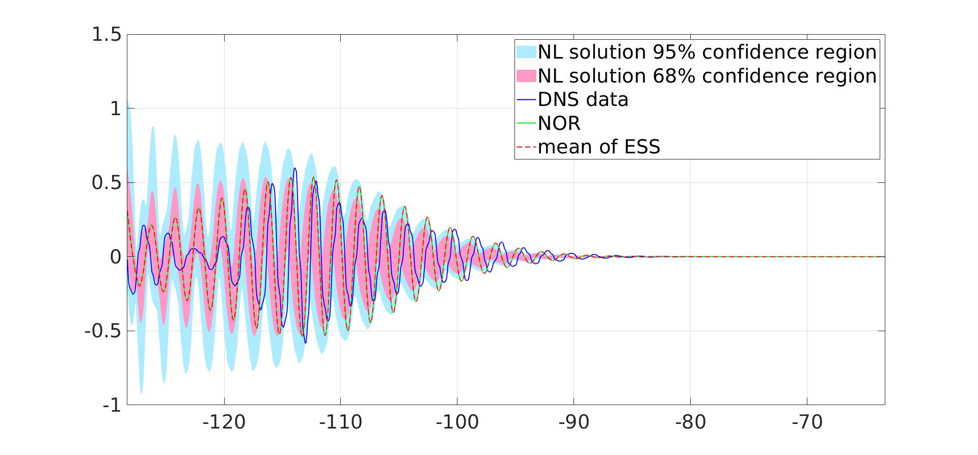
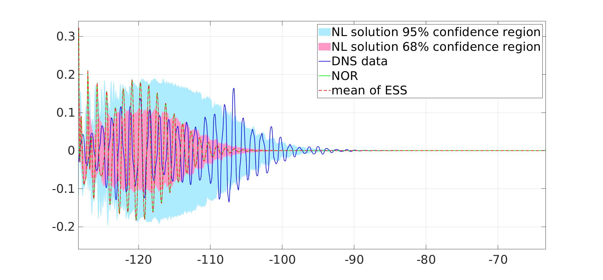
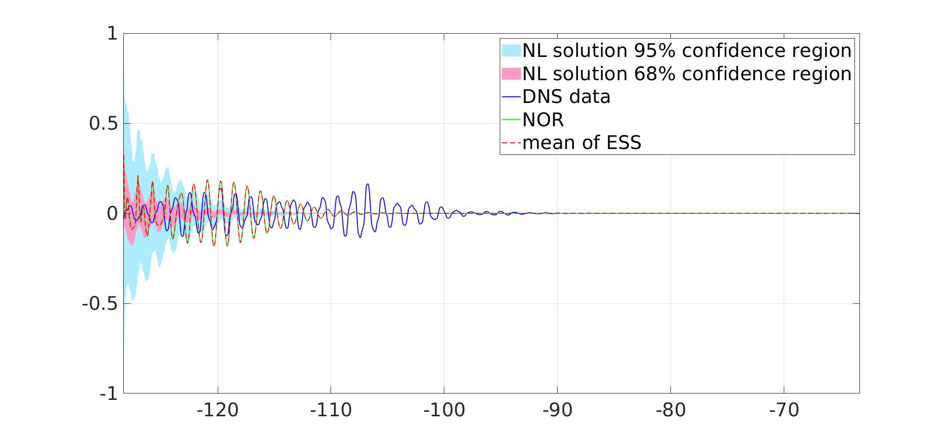
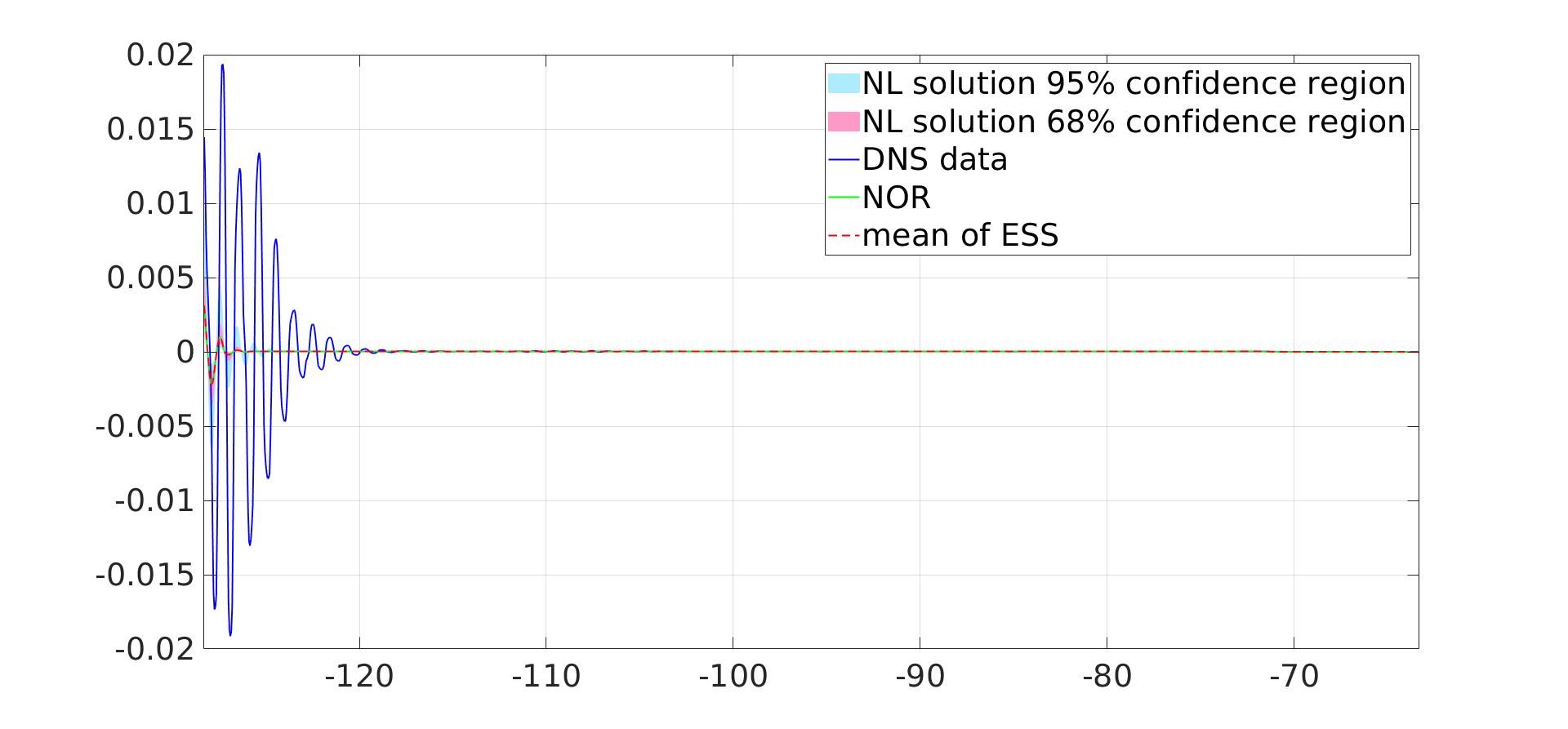
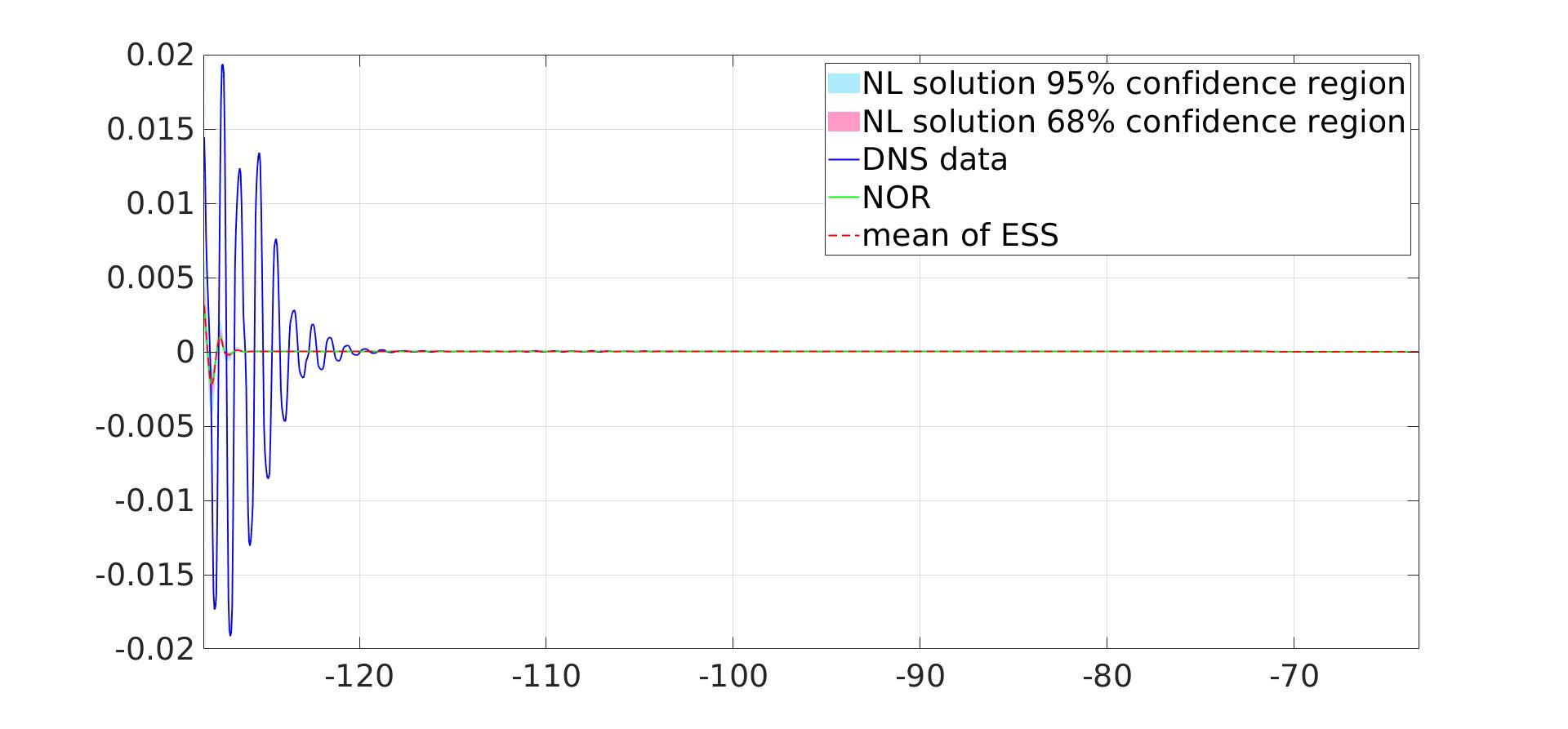
Finally, we provide the prediction of a wave packet, a waveform that is substantially different from the training data. With this setting, we consider an extrapolation scenario: the learnt model is employed to generate a long-term simulation up to , which is the training time interval. In Fig.9, we plot the results using and . For a low-frequency wave (), works better, in the sense that the predictive distribution more closely follows the small features of the wave, roughly reflecting the local magnitude of the discrepancy between the two solutions. On the other hand, the case with fails to do so, with a predictive distribution that broadly encompasses the two solutions, but does not capture the small-scale structure. In both cases, the confidence region fully covers the ground truth, providing a conservative estimation of uncertainty, and avoiding overconfidence, as is the intent of the embedded model error construction. Considering next the case, a frequency close to the band gap, we find that the larger correlation length provides better predictions. Here, the case with smaller correlation length suffers from a mismatch between the uncertainty prediction, the single push-forward of the mean of ESS, and the ground truth. This observation is consistent with the results in Fig.7, where the band gap shifts from the ground-truth band gap and the confidence region fails to cover the DNS data. For the frequency () that is much larger than the band gap frequency, the stress wave is anticipated to stop propagating. In this setting we find that both small and large correlation length cases work well. The best values for the validation samples are also provided in Fig.10, where the optimal correlation length varies depending on the frequency and wave type.
In conclusion, the correlation length for the embedded model error impacts the results differently for different waves, so that the optimal choice would need to be selected according to the purpose of the task. A frequency/waveform-dependent might be of interest. We leave this as a possible future direction. In the following, we choose the best according to the fidelity of prediction of group velocity in Fig.7, choosing as the optimal correlation length.
4.1.3 Comparison with the Baseline
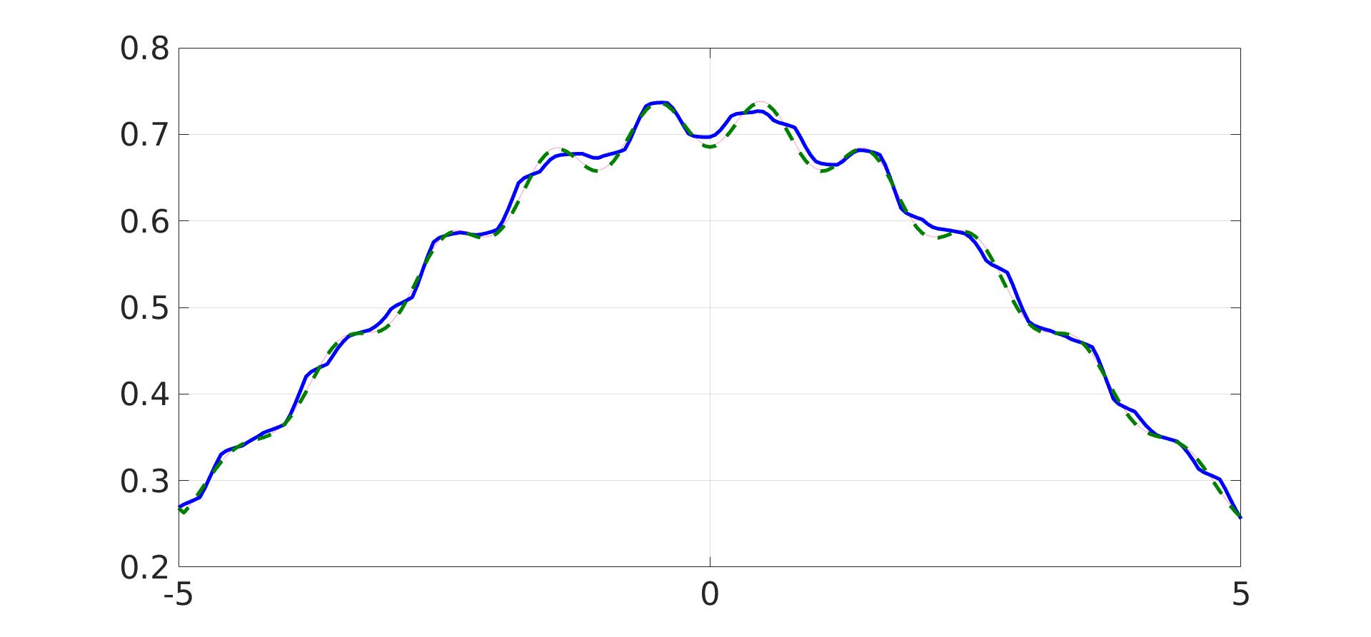
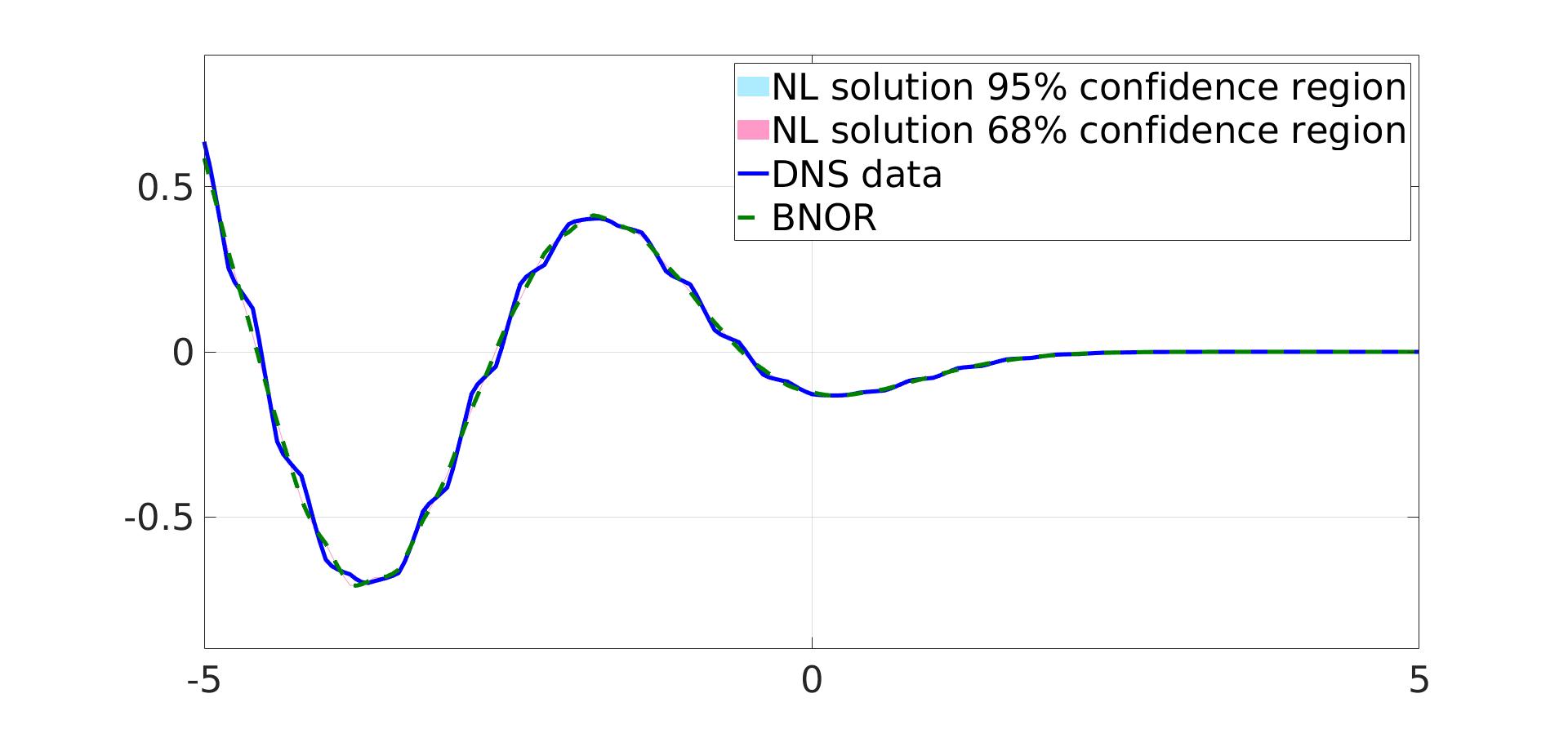
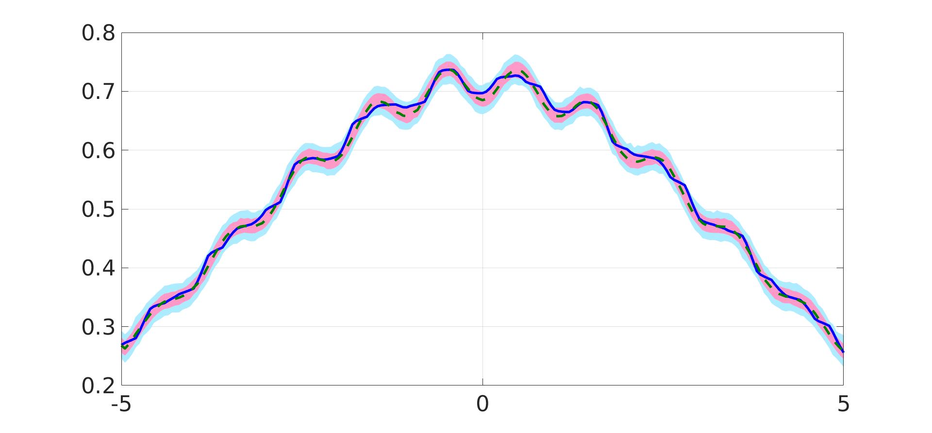
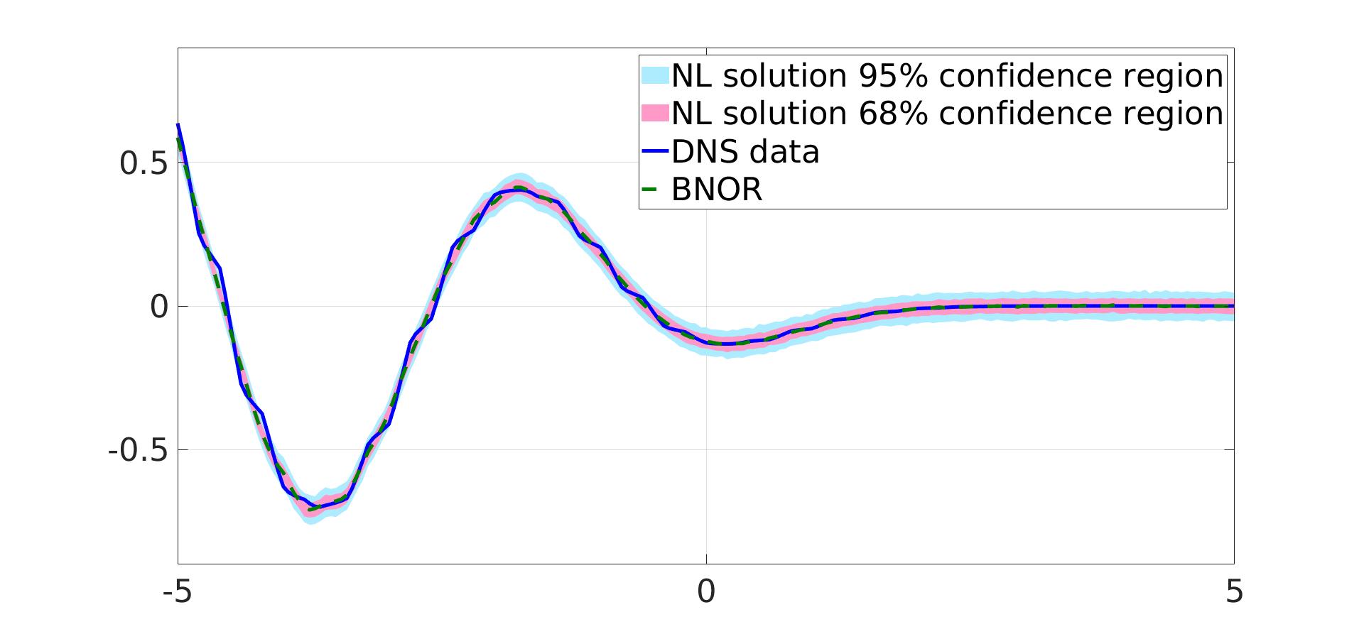
To further illustrate the efficacy of the present ENOR construction in capturing model error, we compare the posterior uncertainty on model predictions (with ) to the results from BNOR [47], where an additive iid noise model was used. Results are shown in Fig.11 for two training data samples at a given time instant . We compare the equivalent PP/PFP ENOR results with the corresponding BNOR PP and PFP results. From Figs.11 (c) and (d), one can see that the BNOR PFP exhibits an almost negligible confidence region. On the other hand, the BNOR PP, shown in Figs.11 (e) and (f), exhibits higher uncertainty with a uniform-width confidence region around the mean prediction, as is expected given the additive iid noise. Compared with these two baseline results, the uncertainty given by the ENOR PP/PFP, shown in Figs.11 (a) and (b), is somewhat more adaptive, exhibiting a degree of uncertainty that approximately tracks the discrepancy between the mean prediction and the DNS data, highlighting the effectiveness of the embedded model error setting. To provide a further quantitative comparison, we note that the BNOR results at in [47] exhibit a PFP CRPS of 0.051 and a PP CRPS of 0.039, which are both roughly 10 higher than the present ENOR result in the worst case (CRPS of 0.0048). This again illustrates that the ENOR model provides an uncertainty that better reflects the discrepancy between the mean model prediction and the ground truth.
4.1.4 Parametric Uncertainty versus Model Error
It is instructive to examine the role of parametric uncertainty versus model error in the resulting uncertainty in model predictions. We illustrate in Fig.12 the posterior predictive uncertainty under the following three scenarios.
-
1.
In plots (a) and (b), we consider uncertainty from all sources, by sampling realizations from both the embedded error correction term and the marginal distribution on kernel parameters.
-
2.
In plots (c) and (d), we consider the uncertainty from the embedded error correction term only, using deterministic kernel parameters.
-
3.
In plots (e) and (f), we neglect the embedded error correction term but sample the kernel parameter from the learnt marginal distribution. As such, only the uncertainty from the marginal distribution on kernel parameters is considered.
By comparing the confidence regions from these three settings, one can observe that results from scenarios 1 and 2 almost coincide, while the predicted uncertainty in scenario 3 is negligible. This indicates that nearly all of the predictive uncertainty comes from the embedded model error. This is typical in Bayesian estimation of one model against another in the absence of data noise and when there is a sufficiently large amount of data.
4.2 Example 2: Random Microstructure
To investigate the performance of the ENOR model on more complicated microstructures, we consider here a disordered heterogeneous bar, where the layer lengths of the two materials are random. In particular, the layer sizes are two uniformly distributed random variables: , with the average layer size and the disorder parameter . The density for both components is still set as and their Young’s moduli are set at and .
To generate the training dataset, we consider the high-fidelity data under the same settings as in data types 1 and 2 of the periodic bar case. Compared with the periodic microstructure case, from the group velocity generated by the DNS simulations we note that the band stop generally occurs at a lower frequency in the random microstructure case. In fact, for the microstructure considered here, an estimated band stop frequency can be obtained from the DNS simulations. Therefore, for the validation data set, we study wave packets with frequencies and , with the purpose of investigating the performance of our nonlocal surrogate model when the loading frequencies are below (), around (), and above () the estimated band stop frequency .
4.2.1 Results from MCMC Experiments
To demonstrate the convergence of MCMC in this case, we again pick correlation length as an example case to test the utility of ENOR in disordered materials. Following the same settings of the periodic microstructure study, we run 6 independent chains. The results pass the same convergence check both visually and quantitatively, where the improved statistics for all the 24 parameters are very close to , with a maximum of , which again verifies the convergence. The chains provide 24,000 draws in total, with approximately acceptance rate on average and the combined chain shows good mixing. Compared with the periodic bar with inferred , a slightly larger kernel variation, , is obtained here. That suggests that the randomness in the material with disordered microstructure results in a larger model discrepancy relative to the DNS results.
4.2.2 Impact of GP Correlation Length
We now study the impact of different correlation length () values in the disordered material, again considering values ranging from to . In Fig.13, we observe that the uncertainty in the kernel with an embedded GP, , has the same pattern of mean and confidence region variation as in the periodic bar case, given the same random kernel structure and GP properties. In Fig.14, we investigate the behavior of the group velocity, and observe that a larger correlation length provides better fitting of the group velocity, and that reducing the correlation length results in a left shift of the band gap in prediction. While this trend was also observed in the periodic microstructure case (see Fig.7), severer oscillations and larger confidence regions are observed at low frequencies here in the small correlation length case, possibly because of the higher uncertainty levels introduced by the disordered microstructure in the material. In Figs.14 (b) and (d), we show the dispersion curves of the learnt kernels, noting again that positivity of all dispersion curves indicates physical stability of the learnt models.
Finally, we provide again the prediction of a wave packet for a larger domain and longer time as a validation, not present in the training set. Overall, the same conclusion on the correlation length as section 4.1.2 can be reached for disordered material. We refer the reader to Fig18 in Appendix for more details on this experiment. In Fig.15, we provide the best for all the training and validation samples according to the value of the CRPS. Note that the optimal s are different from the ones illustrated in Fig.10, highlighting the dependence of the optimal on the material microstructure.
4.2.3 Comparison with the Baseline
Comparing the CRPS for the posterior PDF on the learnt ENOR model predictions with , to that from the baseline model (BNOR) [47], at the same time instant , we find again superior performance from the present construction. Specifically, the ENOR CRPS is 0.008 while the BNOR PFP and PP CRPS values are 0.041 and 0.025 respectively. Thus, consistent with the findings in the periodic material, the BNOR CRPS values are much higher than the ENOR CRPS, again indicating that the embedded model error construction provides a better statistical fit for the DNS data.
Further, in Fig.16 we compare the posterior predictive density from ENOR and the BNOR PFP/PP densities for two samples from two wave types at . While ENOR again provides a better prediction for solution uncertainty, the confidence region is significantly larger, especially in Fig.16(a). Note that according to Table.1 and Fig.15, is best for sample 10 in wave type 1, while is best for sample 3 in wave type 2. Thus, the correlation length employed here is not ideal for both samples. This again suggests that different correlation length should ideally be employed for different loading scenarios. When comparing the level of solution uncertainty from periodic (see Fig.11 (a) and (b)) and disordered materials (Fig.16 (a) and (b)), a larger confidence region is observed in the later case. In fact, the average standard deviation over the bar in sample 10 of data setting 1 is in the periodic microstructure case and in the disordered case. Similarly, the average standard deviations in sample 3 are and for the periodic and disordered microstructure cases, respectively. These results highlight the increase in uncertainty when randomness is introduced in the microstructure.


4.2.4 Parametric Uncertainty versus Model Error
With the purpose of investigating the impact of different source of uncertainty, we examine the predictive uncertainty resulting from parametric uncertainty versus model error for the disordered material, following the same steps in section 4.1.4. As shown in Fig.17, the embedded model error again dominates the posterior uncertainty, with a negligible role for parametric uncertainty.

5 Conclusion
In this work, we proposed ENOR, a novel Bayesian embedded model error framework, to learn the optimal nonlocal surrogate for multiscale homogenization while also characterizing the impact of model error on predictive uncertainty. When learning the bottom-up nonlocal surrogate from microscale simulations, we find that the best fit surrogate has unavoidable discrepancy from the microscale model, rendering a model error UQ study necessary. While the prior work [47] focused on an additive iid error construction, we here introduce, for the first time, an embedded model error representation in nonlocal operator learning, capturing the impact of model error on predictive uncertainty. The algorithm is developed by adding a Gaussian process to the nonlocal kernel, such that the kernel parameters and the Gaussian process parameters can be inferred simultaneously. To solve the Bayesian inference problem, a two phase algorithm, Alg.1, and a multilevel delayed acceptance Markov chain Monte Carlo (MLDA-MCMC) method are proposed, to provide efficient sampling and fast converging chains. The effectiveness of ENOR is demonstrated on the stress wave propagation problem in heterogeneous bars. Comparing to the prior work [47], ENOR improves the accuracy in (1) capturing the correct group velocity; (2) producing high-fidelity training data and predicting the substantially different wave type with accurate confidence region structure; (3) posterior sampling of the model parameters; and (4) selection for the correlation length for different tasks.
From both visual inspection and quantitative tests, it was observed that the optimal choice of the GP correlation length may differ for different frequencies and wave types. As a natural extension, we plan to investigate frequency-dependent models. We also plan to explore uncertainty quantification for more complex data-driven homogenization models, such as peridynamics models [22, 23] in 2D or 3D, and nonlinear models based on neural networks [42, 34, 91]. Since the number of trainable parameters increases substantially in these models, efficient Bayesian inference techniques and reduced order error models would be desired.
Acknowledgements
YF and YY acknowledge support by the National Science Foundation under award DMS-2436624, the National Institute of Health under award 1R01GM157589-01, and the AFOSR grant FA9550-22-1-0197. Portions of this research were conducted on Lehigh University’s Research Computing infrastructure partially supported by NSF Award 2019035. HNN acknowledges the support of the U.S. Department of Energy, Office of Science, Office of Advanced Scientific Computing Research (ASCR), Scientific Discovery through Advanced Computing (SciDAC) Program through the FASTMath Institute. Sandia National Laboratories is a multi-mission laboratory managed and operated by National Technology & Engineering Solutions of Sandia, LLC (NTESS), a wholly owned subsidiary of Honeywell International Inc., for the U.S. Department of Energy’s National Nuclear Security Administration (DOE/NNSA) under contract DE-NA0003525. This written work is authored by an employee of NTESS. The employee, not NTESS, owns the right, title and interest in and to the written work and is responsible for its contents. Any subjective views or opinions that might be expressed in the written work do not necessarily represent the views of the U.S. Government. The publisher acknowledges that the U.S. Government retains a non-exclusive, paid-up, irrevocable, world-wide license to publish or reproduce the published form of this written work or allow others to do so, for U.S. Government purposes. The DOE will provide public access to results of federally sponsored research in accordance with the DOE Public Access Plan.
6 Appendix
6.1 Additional Results
In Figure 18, we provide the validation results using and on wave packet for the random microstructure material, at the last time step . At low frequencies (), works better in reflecting the local magnitude of the solution discrepancy. Near the band stop (), works better since the confidence region from the small case fails to cover the DNS data. For the large frequency case (), both ENOR models have successfully predicted that the stress wave should stop propagating. These observations are consistent with the results from the periodic microstructure material.
References
- [1] Tarek I Zohdi. Homogenization methods and multiscale modeling. Encyclopedia of Computational Mechanics Second Edition, pages 1–24, 2017.
- [2] Alain Bensoussan, Jacques-Louis Lions, and George Papanicolaou. Asymptotic analysis for periodic structures, volume 374. American Mathematical Soc., 2011.
- [3] E Weinan and Bjorn Engquist. Multiscale modeling and computation. Notices of the AMS, 50(9):1062–1070, 2003.
- [4] Yalchin Efendiev, Juan Galvis, and Thomas Y Hou. Generalized multiscale finite element methods (gmsfem). Journal of computational physics, 251:116–135, 2013.
- [5] Christoph Junghans, Matej Praprotnik, and Kurt Kremer. Transport properties controlled by a thermostat: An extended dissipative particle dynamics thermostat. Soft Matter, 4(1):156–161, 2008.
- [6] Rep Kubo. The fluctuation-dissipation theorem. Reports on progress in physics, 29(1):255, 1966.
- [7] Fadil Santosa and William W Symes. A dispersive effective medium for wave propagation in periodic composites. SIAM Journal on Applied Mathematics, 51(4):984–1005, 1991.
- [8] Matthew Dobson, Mitchell Luskin, and Christoph Ortner. Sharp stability estimates for the force-based quasicontinuum approximation of homogeneous tensile deformation. Multiscale Modeling & Simulation, 8(3):782–802, 2010.
- [9] M Ortiz. A method of homogenization of elastic media. International journal of engineering science, 25(7):923–934, 1987.
- [10] Nicolas Moës, J Tinsley Oden, Kumar Vemaganti, and Jean-François Remacle. Simplified methods and a posteriori error estimation for the homogenization of representative volume elements (rve). Computer methods in applied mechanics and engineering, 176(1-4):265–278, 1999.
- [11] Thomas JR Hughes, Garth N Wells, and Alan A Wray. Energy transfers and spectral eddy viscosity in large-eddy simulations of homogeneous isotropic turbulence: Comparison of dynamic smagorinsky and multiscale models over a range of discretizations. Physics of Fluids, 16(11):4044–4052, 2004.
- [12] Graeme W Milton. The theory of composites. SIAM, 2022.
- [13] S Jonathan Chapman and Zachary M Wilmott. Homogenization of flow through periodic networks. SIAM Journal on Applied Mathematics, 81(3):1034–1051, 2021.
- [14] Pep Espanol and Patrick Warren. Statistical mechanics of dissipative particle dynamics. Europhysics letters, 30(4):191, 1995.
- [15] Robert D Groot and Patrick B Warren. Dissipative particle dynamics: Bridging the gap between atomistic and mesoscopic simulation. The Journal of chemical physics, 107(11):4423–4435, 1997.
- [16] PJ Hoogerbrugge and JMVA Koelman. Simulating microscopic hydrodynamic phenomena with dissipative particle dynamics. Europhysics letters, 19(3):155, 1992.
- [17] MJ Beran and JJ McCoy. Mean field variations in a statistical sample of heterogeneous linearly elastic solids. International Journal of Solids and Structures, 6(8):1035–1054, 1970.
- [18] Kirill Cherednichenko, Valery P Smyshlyaev, and VV Zhikov. Non-local homogenised limits for composite media with highly anisotropic periodic fibres. Proceedings of the Royal Society of Edinburgh Section A Mathematics, 136(1):87–114, 2006.
- [19] Frank C Karal Jr and Joseph B Keller. Elastic, electromagnetic, and other waves in a random medium. Journal of Mathematical Physics, 5(4):537–547, 1964.
- [20] Y Rahali, I Giorgio, JF Ganghoffer, and Francesco dell’Isola. Homogenization à la piola produces second gradient continuum models for linear pantographic lattices. International Journal of Engineering Science, 97:148–172, 2015.
- [21] Stewart A Silling. Propagation of a stress pulse in a heterogeneous elastic bar. Journal of Peridynamics and Nonlocal Modeling, 3(3):255–275, 2021.
- [22] Huaiqian You, Yue Yu, Stewart Silling, and Marta D’Elia. A data-driven peridynamic continuum model for upscaling molecular dynamics. Computer Methods in Applied Mechanics and Engineering, 389:114400, 2022.
- [23] HQ You, Xiao Xu, Yue Yu, Stewart Silling, Marta D’Elia, and John Foster. Towards a unified nonlocal, peridynamics framework for the coarse-graining of molecular dynamics data with fractures. Applied Mathematics and Mechanics, 44(7):1125–1150, 2023.
- [24] Huaiqian You, Yue Yu, Stewart Silling, and Marta D’Elia. Nonlocal operator learning for homogenized models: From high-fidelity simulations to constitutive laws. Journal of Peridynamics and Nonlocal Modeling, pages 1–16, 2024.
- [25] Lu Zhang, Huaiqian You, and Yue Yu. MetaNOR: A meta-learnt nonlocal operator regression approach for metamaterial modeling. MRS Communications, 2022.
- [26] Eitan Tadmor and Changhui Tan. Critical thresholds in flocking hydrodynamics with non-local alignment. Philosophical Transactions of the Royal Society A: Mathematical, Physical and Engineering Sciences, 372(2028):20130401, 2014.
- [27] Qiang Du, Bjorn Engquist, and Xiaochuan Tian. Multiscale modeling, homogenization and nonlocal effects: Mathematical and computational issues. Contemporary mathematics, 754, 2020.
- [28] Stewart A Silling. Reformulation of elasticity theory for discontinuities and long-range forces. Journal of the Mechanics and Physics of Solids, 48(1):175–209, 2000.
- [29] Guy Gilboa and Stanley Osher. Nonlocal operators with applications to image processing. Multiscale Modeling & Simulation, 7(3):1005–1028, 2009.
- [30] E. Scalas, R. Gorenflo, and F. Mainardi. Fractional calculus and continuous time finance. Physica A, 284:376–384, 2000.
- [31] M. D’Elia, Q. Du, M. Gunzburger, and R. Lehoucq. Nonlocal convection-diffusion problems on bounded domains and finite-range jump processes. Computational Methods in Applied Mathematics, 29:71–103, 2017.
- [32] M. Meerschaert and A. Sikorskii. Stochastic models for fractional calculus. Studies in mathematics, Gruyter, 2012.
- [33] Stewart A Silling, Siavash Jafarzadeh, and Yue Yu. Peridynamic models for random media found by coarse graining. Journal of Peridynamics and Nonlocal Modeling, pages 1–30, 2024.
- [34] Siavash Jafarzadeh, Stewart Silling, Lu Zhang, Colton Ross, Chung-Hao Lee, SM Rahman, Shuodao Wang, and Yue Yu. Heterogeneous peridynamic neural operators: Discover biotissue constitutive law and microstructure from digital image correlation measurements. arXiv preprint arXiv:2403.18597, 2024.
- [35] Valery P Smyshlyaev and Kirill D Cherednichenko. On rigorous derivation of strain gradient effects in the overall behaviour of periodic heterogeneous media. Journal of the Mechanics and Physics of Solids, 48(6-7):1325–1357, 2000.
- [36] John R Willis. The nonlocal influence of density variations in a composite. International Journal of Solids and Structures, 21(7):805–817, 1985.
- [37] A. C. Eringen and D. G. B. Edelen. On nonlocal elasticity. International Journal of Engineering Science, 10(3):233–248, 1972.
- [38] Florin Bobaru, John T Foster, Philippe H Geubelle, and Stewart A Silling. Handbook of peridynamic modeling. CRC press, 2016.
- [39] Huaiqian You, Yue Yu, Stewart Silling, and Marta D’Elia. Data-driven learning of nonlocal models: from high-fidelity simulations to constitutive laws. AAAI Spring Symposium: MLPS, 2021.
- [40] Huaiqian You, Yue Yu, Nathaniel Trask, Mamikon Gulian, and Marta D’Elia. Data-driven learning of nonlocal physics from high-fidelity synthetic data. Computer Methods in Applied Mechanics and Engineering, 374:113553, 2021.
- [41] Xiao Xu, Marta D’Elia, and John T Foster. A machine-learning framework for peridynamic material models with physical constraints. Computer Methods in Applied Mechanics and Engineering, 386:114062, 2021.
- [42] Siavash Jafarzadeh, Stewart Silling, Ning Liu, Zhongqiang Zhang, and Yue Yu. Peridynamic neural operators: A data-driven nonlocal constitutive model for complex material responses. arXiv preprint arXiv:2401.06070, 2024.
- [43] Eduardo A Barros de Moraes, Marta D’Elia, and Mohsen Zayernouri. Machine learning of nonlocal micro-structural defect evolutions in crystalline materials. Computer Methods in Applied Mechanics and Engineering, 403:115743, 2023.
- [44] Xiao Xu, Marta D’Elia, Christian Glusa, and John T Foster. Machine-learning of nonlocal kernels for anomalous subsurface transport from breakthrough curves. arXiv preprint arXiv:2201.11146, 2022.
- [45] Yue Yu, Ning Liu, Fei Lu, Tian Gao, Siavash Jafarzadeh, and Stewart Silling. Nonlocal attention operator: Materializing hidden knowledge towards interpretable physics discovery. arXiv preprint arXiv:2408.07307, 2024.
- [46] Fei Lu, Qingci An, and Yue Yu. Nonparametric learning of kernels in nonlocal operators. arXiv preprint arXiv:2205.11006, 2022.
- [47] Yiming Fan, Marta D’Elia, Yue Yu, Habib N Najm, and Stewart Silling. Bayesian nonlocal operator regression: A data-driven learning framework of nonlocal models with uncertainty quantification. Journal of Engineering Mechanics, 149(8):04023049, 2023.
- [48] M. de Laplace. Essai philosophique sur les probabilités. Gauthier-Villars, Paris, 1814. English Ed.: "A Philosophical Essay on Probabilities", Dover Pub., 6th ed., 1995.
- [49] George Casella and Roger L Berger. Statistical inference, volume 70. Duxbury Press Belmont, CA, 1990.
- [50] E.T. Jaynes. Probability Theory: The Logic of Science, G.L. Bretthorst, Ed. Cambridge University Press, Cambridge, UK, 2003.
- [51] C.P. Robert and G. Casella. Monte Carlo Statistical Methods. Springer Texts in Statistics. Springer, 2004.
- [52] D. S. Sivia and J. Skilling. Data Analysis: A Bayesian Tutorial, Second Edition. Oxford University Press, 2006.
- [53] B. P. Carlin and T. A. Louis. Bayesian Methods for Data Analysis. Chapman and Hall/CRC, Boca Raton, FL, 2011.
- [54] M. C. Kennedy and A. O’Hagan. Bayesian calibration of computer models. Journal of the Royal Statistical Society: Series B, 63(3):425–464, 2001.
- [55] D. Higdon, H. Lee, and C. Holloman. Markov chain Monte Carlo-based approaches for inference in computationally intensive inverse problems. Bayesian Statistics, 7:181–197, 2003.
- [56] T. A. Oliver and R. D. Moser. Bayesian uncertainty quantification applied to RANS turbulence models. J. Phys.: Conf. Ser., 318, 2011.
- [57] Tiangang Cui, Youssef Marzouk, and Karen Willcox. Scalable posterior approximations for large-scale Bayesian inverse problems via likelihood-informed parameter and state reduction. Journal of Computational Physics, 315:363–387, 2016.
- [58] Layal Hakim, Guilhem Lacaze, Mohammad Khalil, Khachik Sargsyan, Habib Najm, and Joseph Oefelein. Probabilistic parameter estimation in a 2-step chemical kinetics model for n-dodecane jet autoignition. Combustion Theory and Modelling, 22(3):446–466, 2018.
- [59] Xun Huan, Cosmin Safta, Khachik Sargsyan, Gianluca Geraci, Michael S. Eldred, Zachary P. Vane, Guilhem Lacaze, Joseph C. Oefelein, and Habib N. Najm. Global Sensitivity Analysis and Estimation of Model Error, toward Uncertainty Quantification in Scramjet Computations. AIAA Journal, 56(3):1170–1184, 2018.
- [60] Maria J Bayarri, James O Berger, Rui Paulo, Jerry Sacks, John A Cafeo, James Cavendish, Chin-Hsu Lin, and Jian Tu. A framework for validation of computer models. Technometrics, 49(2):138–154, 2007.
- [61] Jack PC Kleijnen. Kriging metamodeling in simulation: A review. European journal of operational research, 192(3):707–716, 2009.
- [62] K Sargsyan, HN Najm, and R Ghanem. On the statistical calibration of physical models. International Journal of Chemical Kinetics, 47(4):246–276, 2015.
- [63] Khachik Sargsyan, Xun Huan, and Habib N Najm. Embedded model error representation for bayesian model calibration. International Journal for Uncertainty Quantification, 9(4), 2019.
- [64] Mikkel B. Lykkegaard, Grigorios Mingas, Robert Scheichl, Colin Fox, and Tim J. Dodwell. Multilevel delayed acceptance mcmc with an adaptive error model in pymc3, 2020. Workshop on machine learning for engineering modeling, simulation and design, NeurIPS 2020.
- [65] Mikkel B Lykkegaard, Tim J Dodwell, Colin Fox, Grigorios Mingas, and Robert Scheichl. Multilevel delayed acceptance mcmc. SIAM/ASA Journal on Uncertainty Quantification, 11(1):1–30, 2023.
- [66] Ning Liu, Yue Yu, Huaiqian You, and Neeraj Tatikola. Ino: Invariant neural operators for learning complex physical systems with momentum conservation. In International Conference on Artificial Intelligence and Statistics, pages 6822–6838. PMLR, 2023.
- [67] Ning Liu, Yiming Fan, Xianyi Zeng, Milan Klöwer, LU ZHANG, and Yue Yu. Harnessing the power of neural operators with automatically encoded conservation laws. In Forty-first International Conference on Machine Learning, 2024.
- [68] Qiang Du, Yunzhe Tao, and Xiaochuan Tian. A peridynamic model of fracture mechanics with bond-breaking. Journal of Elasticity, pages 1–22, 2017.
- [69] M. C. Kennedy and A. O’Hagan. Bayesian calibration of computer models (with discussion). Journal of the Royal Statistical Society B, 63:425–464, 2001.
- [70] M. C. Kennedy, A. O’Hagan, and N. Higgins. Bayesian analysis of computer code outputs. In Quantitative Methods for Current Environmental Issues. C. W. Anderson, V. Barnett, P. C. Chatwin, and A. H. El-Shaarawi (eds.), pages 227–243. Springer-Verlag: London, 2002.
- [71] D. Higdon, M. C. Kennedy, J. Cavendish, J. Cafeo, and R. D. Ryne. Combining field data and computer simulations for calibration and prediction. SIAM Journal on Scientific Computing, 26:448–466, 2004.
- [72] M. J. Bayarri, J. O. Berger, M. C. Kennedy, A. Kottas, R. Paulo, J. Sacks, J. A. Cafeo, C. H. Lin, and J. Tu. Predicting vehicle crashworthiness: validation of computer models for functional and hierarchical data. Journal of the American Statistical Association, 104:929–942, 2009.
- [73] Layal Hakim, Guilhem Lacaze, Mohammad Khalil, Khachik Sargsyan, Habib Najm, and Joseph Oefelein. Probabilistic parameter estimation in a 2-step chemical kinetics model for n-dodecane jet autoignition. Combustion Theory and Modelling, 22(3):446–466, 2018.
- [74] Xun Huan, Cosmin Safta, Khachik Sargsyan, Gianluca Geraci, Michael S. Eldred, Zachary P. Vane, Guilhem Lacaze, Joseph C. Oefelein, and Habib N. Najm. Global sensitivity analysis and estimation of model error, toward uncertainty quantification in scramjet computations. AIAA Journal, 56(3):1170–1184, 2018.
- [75] Arun Hegde, Elan Weiss, Wolfgang Windl, Habib N. Najm, and Cosmin Safta. A bayesian calibration framework with embedded model error for model diagnostics. International Journal for Uncertainty Quantification, 14(6):37–70, 2024.
- [76] M. Beaumont, W. Zhang, and D. J. Balding. Approximate Bayesian Computation in population genetics. Genetics, 162(4):2025–2035, 2002.
- [77] P. Marjoram, J. Molitor, V. Plagnol, and S. Tavaré. Markov chain Monte Carlo without likelihoods. Proc Natl Acad Sci USA, 100(26):15324–15328, 2003.
- [78] S. A. Sisson and Y. Fan. Handbook of Markov Chain Monte Carlo, chapter Likelihood-free Markov chain Monte Carlo, pages 313–338. Chapman and Hall/CRC Press, 2011.
- [79] K. Karhunen. Zur spektraltheorie stochastischer prozesse. Ann. Acad. Sci. Fennicae, 37, 1946.
- [80] Pol D Spanos, Michael Beer, and John Red-Horse. Karhunen–loève expansion of stochastic processes with a modified exponential covariance kernel. Journal of Engineering Mechanics, 133(7):773–779, 2007.
- [81] Didier Lucor, C-H Su, and George Em Karniadakis. Generalized polynomial chaos and random oscillators. International Journal for Numerical Methods in Engineering, 60(3):571–596, 2004.
- [82] Tiangang Cui, Colin Fox, and MJ O’sullivan. Bayesian calibration of a large-scale geothermal reservoir model by a new adaptive delayed acceptance metropolis hastings algorithm. Water Resources Research, 47(10), 2011.
- [83] S Abrate. Wave propagation in lightweight composite armor. In Journal de Physique IV (Proceedings), volume 110, pages 657–662. EDP sciences, 2003.
- [84] Oriol Abril-Pla, Virgile Andreani, Colin Carroll, Larry Dong, Christopher J Fonnesbeck, Maxim Kochurov, Ravin Kumar, Junpeng Lao, Christian C Luhmann, Osvaldo A Martin, et al. Pymc: a modern, and comprehensive probabilistic programming framework in python. PeerJ Computer Science, 9:e1516, 2023.
- [85] Cajo JF Ter Braak and Jasper A Vrugt. Differential evolution markov chain with snooker updater and fewer chains. Statistics and Computing, 18:435–446, 2008.
- [86] Aki Vehtari, Andrew Gelman, Daniel Simpson, Bob Carpenter, and Paul-Christian Bürkner. Rank-normalization, folding, and localization: An improved for assessing convergence of mcmc (with discussion). Bayesian analysis, 16(2):667–718, 2021.
- [87] Dootika Vats, James M Flegal, and Galin L Jones. Multivariate output analysis for markov chain monte carlo. Biometrika, 106(2):321–337, 2019.
- [88] A. Gelman, J.B. Carlin, H.S. Stern, and D.B. Rubin. Bayesian Data Analysis. Chapman and Hall/CRC, London, 1995.
- [89] Andrew Gelman, Xiao-Li Meng, and Hal Stern. Posterior predictive assessment of model fitness via realized discrepancies. Statistica Sinica, 6(4):733–760, 1996.
- [90] Michaël Zamo and Philippe Naveau. Estimation of the continuous ranked probability score with limited information and applications to ensemble weather forecasts. Mathematical Geosciences, 50(2):209–234, 2018.
- [91] Huaiqian You, Quinn Zhang, Colton J Ross, Chung-Hao Lee, and Yue Yu. Learning deep implicit fourier neural operators (ifnos) with applications to heterogeneous material modeling. arXiv preprint arXiv:2203.08205, 2022.