High-dimensional partial linear model with trend filtering
Abstract
We study the high-dimensional partial linear model, where the linear part has a high-dimensional sparse regression coefficient and the nonparametric part includes a function whose derivatives are of bounded total variation. We expand upon the univariate trend filtering (Tibshirani, 2014) to develop partial linear trend filtering–a doubly penalized least square estimation approach based on penalty and total variation penalty. Analogous to the advantages of trend filtering in univariate nonparametric regression, partial linear trend filtering not only can be efficiently computed, but also achieves the optimal error rate for estimating the nonparametric function. This in turn leads to the oracle rate for the linear part as if the underlying nonparametric function were known. We compare the proposed approach with a standard smoothing spline based method (Müller and Van de Geer, 2015; Yu et al., 2019), and show both empirically and theoretically that the former outperforms the latter when the underlying function possesses heterogeneous smoothness. We apply our approach to the IDATA study to investigate the relationship between metabolomic profiles and ultra-processed food (UPF) intake, efficiently identifying key metabolites associated with UPF consumption and demonstrating strong predictive performance.
1 Introduction
We study a widely encountered scenario where the response variable is influenced by two different kinds of predictors, and : the relationship between and is linear while the dependence of on is non-linear. To analyze such types of data, we consider the following partial linear regression model
| (1) |
where is a -dimensional sparse vector of unknown coefficients, is an unknown nonparametric function, and is a zero-mean error. We focus on the setting in which the dimension is comparable to or much larger than the sample size and the predictor is univariate111We discuss the generalization to the case in Section 5.. This high-dimensional partial linear regression model plays an important role in big data analytics as it combines the flexibility of nonparametric regression and parsimony of linear regression. It finds applications in diverse fields ranging from genomics and health sciences to economics and finance. For example, in many biological studies, is often a high-dimensional vector encoding genetic information, while the predictor contains the measurements of clinical or environment variables, such as age and weight.
The model (1) has been extensively studied when the dimension of is fixed or small relative to ; see, for example, Engle et al. (1986); Chen (1988); Wahba (1990); Mammen and van de Geer (1997); Härdle et al. (2000); Bunea (2004); Xie and Huang (2009). Its high-dimensional extensions have been further considered in Müller and Van de Geer (2015); Ma and Huang (2016); Zhu (2017); Yu et al. (2019); Zhu et al. (2019); Lv and Lian (2022); Fu et al. (2024a). Among the aforementioned works, a commonly-used approach is to combine penalization techniques such as LASSO (Tibshirani, 1996) and SCAD (Fan and Li, 2001) for the parametric part (if is sparse), with classical nonparametric methods such as splines and local polynomial smoothing for the estimation of . And the underlying function is typically assumed to belong to a Sobolev or Holder function class. In particular, when is from -order Sobolev class and is a high-dimensional vector with sparsity , Müller and Van de Geer (2015) showed that using doubly penalized least square estimators, the linear parametric part can be estimated with oracle rates , while the convergence rate for undergoes a phase transition between the sparse estimation rate and the nonparametric rate . Yu et al. (2019) further proved that these rates for and are both minimax optimal.
Despite a rich literature on partial linear regression models, the widely adopted smoothing methods based on local polynomials, kernels and splines can fail to estimate adequately well, when possesses spatially inhomogeneous smoothness (e.g. is smooth in some parts and wiggly in other parts). This issue has been well recognized in classical univariate nonparametric regressions where . Suppose lies in the univariate function class
| (2) |
where TV(·) is the total variation operator, is the th weak derivative of , and is a constant. Note that allows for more heterogeneous smoothness of than Sobolev or Holder classes. The results of Donoho and Johnstone (1998) imply that the minimax estimation rate over is , while the best possible rate attained by any linear smoother is and hence suboptimal. Just as linear smoothers (e.g. local polynomials, smoothing splines, regression splines) do not adapt well to the changes in the local level of smoothness in univariate nonparametric regressions, any estimator of based on linear smoothing ideas in partial linear regressions will suffer from the same problem. To overcome this limitation, we leverage a relatively new nonparametric approach known as trend filtering (Steidl et al., 2006; Kim et al., 2009) to construct favorable estimates for heterogeneously smooth as well as sparse in the high-dimensional partial linear models.
Trend filtering can be described as an approximation to the locally adaptive regression splines introduced by Mammen and Van De Geer (1997). In the univariate nonparametric regressions, the locally adaptive regression spline estimator is the solution of the following total variation regularized problem:
| (3) |
where is a tuning parameter. Mammen and Van De Geer (1997) proved that the solution in (3) achieves the minimax estimation rate over , so it adapts to the local level of smoothness significantly better than any linear smoothers. Mammen and Van De Geer (1997) also showed that the solution is a th degree spline, however, its knots could occur at noninput points when and the locations are not easy to determine. To address this computational problem, Mammen and Van De Geer (1997) proposed a restricted version of (3),
| (4) |
where is an -dimensional space of th degree splines with knots all contained in the set of input points. Using basis functions that span (e.g. B-spline or truncated power basis), (4) can be expressed as a finite-dimensional generalized lasso problem (Tibshirani, 2014), thereby computationally more tractable than (3). Moreover, Mammen and Van De Geer (1997) proved that the solution of (4) can still attain the optimal rate over under weak conditions. Trend filtering replaces in (4) with an -dimensional space spanned by spline-like basis functions known as falling factorial basis (see Section 2.1 for details). Tibshirani (2014); Wang et al. (2014); Ramdas and Tibshirani (2016) formally showed that the resulting estimates not only achieve the minimax optimal rate over , but also are much easier to compute than (4) due to certain banded structure in the optimization problem. See Tibshirani (2022) for a comprehensive treatment of falling factorial basis functions and its connections to discrete splines.
The local adaptivity and computational efficiency make trend filtering an attractive nonparametric tool. In recent years, there has been substantial interest and progress in trend filtering for various statistical problems, including univariate nonparametric regression under strong sparsity (Guntuboyina et al., 2020; Ortelli and van de Geer, 2021), graph trend filtering (Wang et al., 2016; Hütter and Rigollet, 2016; Padilla et al., 2018; Ortelli and van de Geer, 2018; Madrid Padilla et al., 2020), functional trend filtering (Wakayama and Sugasawa, 2023), scalar-on-image regression models (Wang et al., 2017), additive models (Sadhanala and Tibshirani, 2019; Petersen and Witten, 2019; Tan and Zhang, 2019), quantile regression models (Ye and Padilla, 2021; Madrid Padilla and Chatterjee, 2022; Wang et al., 2024), and spatiotemporal models (Padilla et al., 2023; Rahardiantoro and Sakamoto, 2024), among others. However, its application within the high-dimensional partial linear model framework has not been explored to date.
In this paper, we extend trend filtering to the high-dimensional partial linear model setting. We use -penalization for the high-dimensional parametric part with sparsity , and utilize trend filtering to estimate the nonparametric function . We prove that our estimate for attains the oracle rate as if were known, and the convergence rate for exhibits a phase transition between and the optimal nonparametric rate . Therefore, our theory generalizes the results in Müller and Van de Geer (2015); Yu et al. (2019) to functions possessing variable spatial smoothness. The proposed estimates can be computed fast via a simple blockwise coordinate descent scheme based on efficient algorithms for univariate trend filtering. We further demonstrate the effectiveness of our method through extensive simulations and real data analyses.
The real data analyses are performed with the Interactive Diet and Activity Tracking in AARP (IDATA) Study, where our aim is to investigate the relationship between metabolomic profiles and ultra-processed food (UPF) intake using serum and urine datasets. Identifying biomarkers of UPF intake is essential because traditional dietary assessment methods, like food frequency questionnaires, are not detailed enough to accurately classify UPFs, which are associated with increased risks of cancer and chronic diseases. Biomarkers, derived from controlled feeding trials, offer a reliable way to assess UPF consumption and its metabolic effects, advancing our understanding of the long-term health impacts of UPFs. We utilize our method to explore associations between UPF consumption and various metabolites. Our method demonstrates strong performance in both prediction and variable selection, providing important insights into potential metabolomic markers related to UPF intake.
The rest of the paper is organized as follows. Section 2 discusses in detail the problem setting, our proposed method and associated theory. Sections 3 and 4 present a thorough simulation study and a real data analysis, respectively. Section 5 gives some concluding remarks. All the proofs are relegated to Section 6.
1.1 Notations
We first clarify the notations used throughout the paper for convenience. We use bold capital letters (e.g. ) to denote matrices, and use bold small letters (e.g. ) to denote vectors. For , denote for and . For two vectors , we write . For a vector and a function , let . Given a square matrix , and represent its largest and smallest eigenvalues respectively. For a general matrix , denotes its spectral norm; . For , . For a set , is the usual indicator function, and to be its cardinality. Moreover, means there exists some constant such that for all ; thus is equivalent to ; if and only if and ; means . We put subscript on and for random variables. For i.i.d. samples from a distribution supported on some space , denote by the associated empirical distribution. The and norms for functions are: . For simplicity we will abbreviate subscripts and write for respectively, whenever is the underlying distribution of the covariates. For a random variable , we also write for . Given random variables , the order statistics are denoted by .
2 Trend filtering in high-dimensional partial linear models
2.1 Problem setting and our method
We consider the partial linear regression model:
where is independent of , has the support with , and is a nonparametric function222Without loss of generality, the support of is assumed as . It can be relaxed to any compact interval.. Let be independent observations of , and denote . We focus on the high-dimensional setting in which the dimension can be much larger than the sample size , and assume with some constant to allow for a large degree of heterogeneous smoothness of .
Expanding upon the univariate trend filtering (Tibshirani, 2014) discussed in Section 1, we consider the following th degree partial linear trend filtering estimation,
| (5) |
where are tuning parameters, and is the span of the th degree falling factorial basis functions defined over the ordered input points . The set of basis functions take the form (Tibshirani, 2014; Wang et al., 2014; Tibshirani, 2022),
| (6) | ||||
| (7) |
where we adopt the convention . The above falling factorial basis look similar to the standard truncated power basis for th degree splines with knots at . In fact, it is straightforward to verify that the two bases are equal when , and they span different spaces when –the falling factorial functions in (7) are piecewise polynomials with discontinuities in their derivatives of orders . Define the matrix with entries . Then for any , we can write for some . The estimation in (5) is thus equivalent to
| (8) |
Further representing and using the formula for (Wang et al., 2014), we can reformulate the optimization (8) as
| (9) |
where is the discrete difference operator of order . When ,
| (10) |
For , the difference operator is defined recursively, that is,
Here, in the above equation is defined as the form of (10) with the dimension of . The problem (9) is a generalized lasso problem. The fact that the penalty matrix is sparse and banded is of great advantage for solving the optimization (9). We defer the computational details to Section 3.1. Once is computed from (9), the estimator in (5) can be obtained as with .
Our estimation approach in (5) introduces a doubly penalized least squares estimator, similar to those proposed by Müller and Van de Geer (2015) and Yu et al. (2019). This approach involves two penalties: the first shrinkage penalty induces sparsity on the parametric part, and the second smoothness penalty controls the complexity of the nonparametric part. The primary distinction between our approach and theirs lies in the estimation method of the function . While both of their methods employ the smoothing spline technique with a squared penalty, our method utilizes trend filtering based on an type penalty which can achieve a finer degree of local adaptivity. Given the structure of partial linear model, a better estimation of is expected to lead to a better estimation of . Therefore, our method improves over the methods in Müller and Van de Geer (2015) and Yu et al. (2019) when possesses heterogeneous smoothness. We will elaborate on this comparison both theoretically and empirically in the following sections.
2.2 Degrees of freedom
In this section, we assume and are fixed with , to study the degrees of freedom for the proposed partial linear trend filtering method (9). Recall that for given data with , the effective degrees of freedom (Stein, 1981; Hastie and Tibshirani, 1990) of , as an estimator of , is defined as
| (11) |
The degrees of freedom measures the complexity of an estimator, and plays an important role in model assessment and selection. Since (9) takes the generalized lasso form, we can apply known results on the generalized lasso (Tibshirani and Taylor, 2011, 2012) to derive the degrees of freedom for (9).
Proposition 1.
Consider from (9). Define the two active sets
Assume the Gaussian partial linear model .
-
(i)
For any fixed and , the degrees of freedom for the fitting is
where is the subspace spanned by the columns of that are indexed by , and is the nullspace of the matrix after removing the rows indexed by .
- (ii)
It is known that is the degrees of freedom for when is a standard lasso estimate (Tibshirani and Taylor, 2012), and is the degrees of freedom for if is from univariate trend filtering (Tibshirani, 2014). Part (i) of Proposition 1 shows that the degrees of freedom for the partial linear trend filtering (9)–based on the idea of combining lasso and trend filtering–equals to the expected dimension of the sum of and . When these two subspaces have no intersection except , the sum becomes direct sum so that
Part (ii) of Proposition 1 provides a sufficient condition for the above to hold. The result in Part (ii) admits a more direct interpretation: for an unbiased estimate of the degrees of freedom of , we count the number of nonzeros in and the number of changes in the th discrete derivative of , and add them up together with .
The degrees of freedom allows us to calibrate model complexities for a fair comparison of different methods. Consider the method from Müller and Van de Geer (2015); Yu et al. (2019) based on smoothing splines,
| (12) |
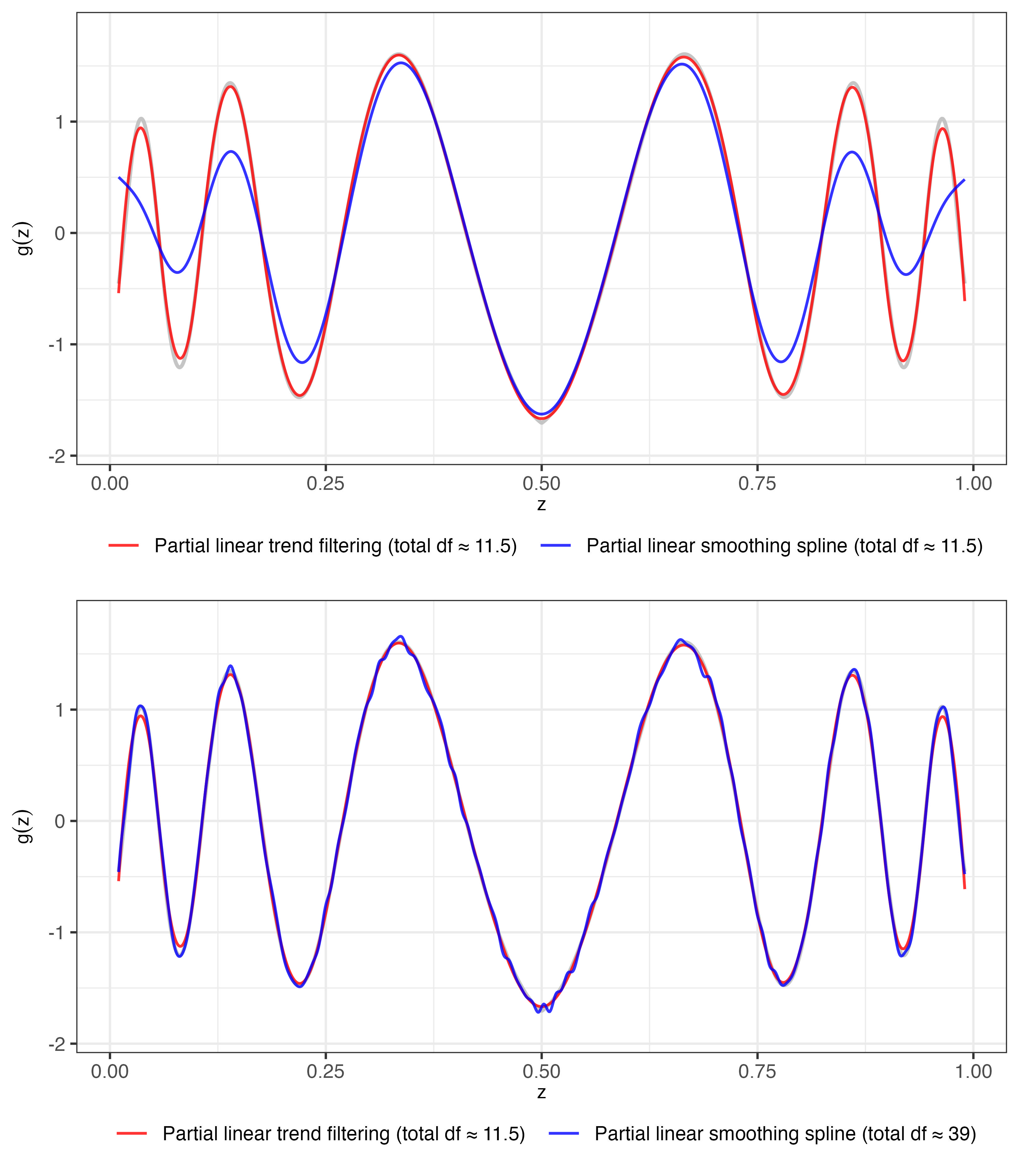
where is the space of th degree natural splines with knots at the input points . We refer to it as partial linear smoothing spline. Using basis functions spanning , the partial linear smoothing spline estimation can be rewritten in a form which is similar to (8) or (9) except that the penalty for the nonparametric part is replaced with a squared penalty. We omit the detail as this is standard in the nonparametrics literature. Figure 1 presents a comparison between the partial linear smoothing spline (12) and partial linear trend filtering (5) across various degrees of freedom333The degrees of freedom for partial linear smoothing spline does not admit a simple form. We hence use the original definition (11) to numerically compute it. (by changing the tuning parameters ). In this comparison, we consider the model with setting and . The figure illustrates that, when both methods are applied with the same total degrees of freedom (11.5), the partial linear smoothing spline fails to adequately capture local smoothness at the function’s boundaries, whereas the partial linear trend filtering method performs more effectively in this regard. Although increasing the degrees of freedom (39) improves the fit of the partial linear smoothing spline at the boundaries, it results in oversmoothing in the central regions of the function. These observations illustrate that partial linear trend filtering adapts to the local level of smoothness better than partial linear smoothing spline. We provide more empirical comparisons in Sections 3 and 4.
2.3 Theory
In this section, we study the rate of convergence for the proposed estimators in (5). We first introduce our technical conditions.
Condition 1.
The covariate has sub-Gaussian coordinates444The sub-Gaussian norm of a random variable is defined as .: .
Condition 2.
The noise is sub-Gaussian: .
Condition 3.
has a continuous distribution supported on . Its density is bounded below by a constant .
Condition 4.
Define and . Assume and .
Condition 5.
Condition 6.
and , as .
Compared to Müller and Van de Geer (2015), Condition 1 relaxes the assumption of from being uniformly bounded to sub-Gaussian. Compared to Yu et al. (2019), Condition 1 only requires sub-Gaussianity for marginal distributions of , instead of the joint distribution. Condition 2 is the same as in Yu et al. (2019), relaxing the errors from being standard normal in Müller and Van de Geer (2015) to sub-Gaussian. For Condition 3, the continuity assumption is very weak, and the lower bound on the density is mainly used to bound the maximum gap between adjacent input points with high probability. See Wang et al. (2014); Sadhanala and Tibshirani (2019) for similar assumptions in the context of trend filtering. Condition 4 is common in semiparametric literature (Yu et al., 2011; Müller and Van de Geer, 2015; Yu et al., 2019). It ensures that there is enough information in the data to identify the parameters in the linear part. Condition 5 is similar to Condition 2.6 in Müller and Van de Geer (2015) and Assumption A.5 in Yu et al. (2019). This condition enables to obtain the fast rate for . Condition 6 is a scaling condition in high dimension. While the main part is stronger than the common assumption in the lasso literature, the gain is to avoid making any joint distribution assumption for . It is possible to only require the weaker condition , if certain distributional assumption (e.g. joint sub-Gaussian) on is made. We leave this for a future study.
Our main results consist of two parts, the result regarding for the nonparametric part, and the result about for the high-dimensional linear part. We now move on to the convergence rate result for .
Theorem 1.
Theorem 1 shows that the integrated squared error and the input-averaged squared error have the same convergence rate, and the rate is determined by the maximum between a sparse estimation rate and a nonparametric rate . When is sufficiently smooth, belonging to a -order Sobolev or Holder class, a similar rate-switching phenomenon (switching between and ) has been revealed for partial linear smoothing spline (12) (Müller and Van de Geer, 2015), and the rate is proved to be (nearly) minimax optimal (Yu et al., 2019). Given that the function class from (2) considered in Theorem 1 is larger than a -order Sobolev class, the minimax lower bound derived for -order Sobolev classes in Yu et al. (2019), i.e. , implies that the rate obtained by our partial linear trend filtering (5) is (nearly) minimax optimal. In particular, when , our method achieves the optimal nonparametric rate that is not attainable by partial linear smoothing spline (see related discussions in Section 1).
We proceed to the convergence rate result for .
Theorem 2.
Theorem 2 demonstrates that the estimation error, out-of-sample prediction error, and in-sample prediction error, all have the same convergence rate . It is well known that this rate is the typical rate that the lasso achieves in standard high-dimensional sparse linear regressions (Tsybakov et al., 2009; Ye and Zhang, 2010; Raskutti et al., 2011; Verzelen, 2012). Therefore, we can conclude that our estimator attains the oracle rate as if the true function were known. Müller and Van de Geer (2015); Yu et al. (2019) showed that the partial linear smoothing spline can achieve the same rate, however, only when lies in Sobolev or Holder classes. In contrast, our method obtains the rate when belongs to a larger class that covers more heterogeneously smooth functions.
3 Simulations
-
1.
Set and initialization
-
2.
For -th iteration, where :
-
(a)
Block 1: Let , and update by fitting the lasso:
-
(b)
Block 2: Let , and update by fitting the univariate trend filtering:
-
(c)
If , then stop the iteration. If not, continue the iteration until it reaches the predefined maximum iteration number
-
(a)
-
3.
Return ( at convergence
Through empirical experiments, we evaluate the performance of partial linear trend filtering (PLTF) introduced in (5), in comparison to partial linear smoothing splines (PLSS) defined in (12) (Müller and Van de Geer, 2015; Yu et al., 2019).
3.1 Computational details
As described in Section 2.1, to compute in (5), we first solve (9) to obtain . Then, , where , and ’s are the falling factorial basis defined in (6)-(7). We use a Block Coordinate Descent (BCD) algorithm for solving the optimization (9). The algorithm iterates over two blocks, and , by solving a standard lasso problem and univariate trend filtering respectively. The detailed steps of the algorithm are outlined in Algorithm 1.
Our algorithm is implemented using R software (R Core Team, 2022). We use R package glmnet (Friedman et al., 2010) to compute the lasso for Block 1 update, and use R package glmgen (Arnold et al., 2014) to compute univariate trend filtering for Block 2 update. We employ warm starts (Friedman et al., 2010; Ramdas and Tibshirani, 2016) to compute solutions over a two-dimensional grid of tuning parameters . A similar strategy is adopted to compute partial linear smoothing splines. The R function, stats::smooth.spline, is used to calculate univariate smoothing spline for Block 2 update. The implemented BCD algorithms for PLTF and PLSS, named plmR, are available on https://sangkyustat.github.io/plmR/ for public use.
3.2 Simulation settings and results
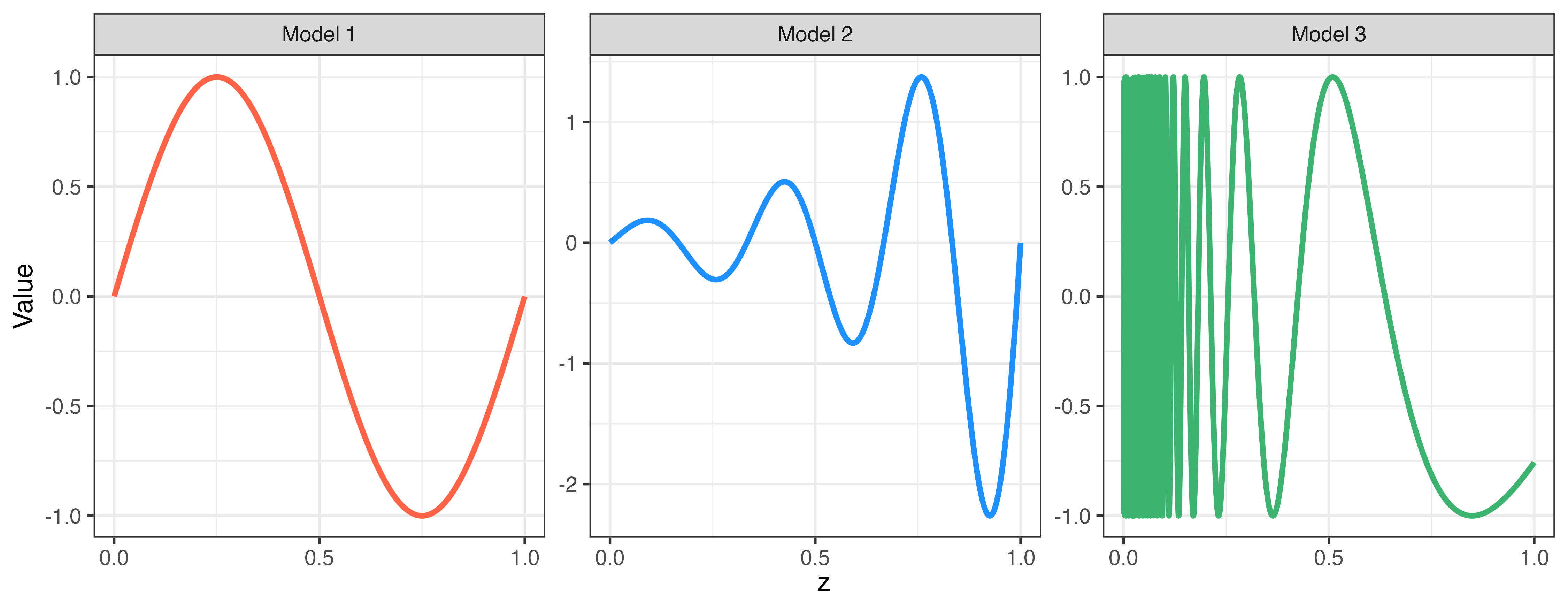
We generate the -dimensional covariates and the univariate covariate in the following way: we first sample from , where with and ; then we set with being the standard normal’s CDF, for , and for . We consider three different partial linear models as follows: for ,
where . The function displays varying levels of heterogeneous smoothness in the three models. The actual forms of these functions are shown in Figure 2. The values for are (0.5, 1, 1, 1.5). Various values for are used to vary the signal-to-noise ratio for the models. Similar to Müller and Van de Geer (2015); Sadhanala and Tibshirani (2019), we define the total signal-to-noise ratio (tSNR) as
We vary the tSNR from 4 to 16 on a logarithmic scale and then calculate the error metrics for each method. Specifically, we consider three different error metrics:
-
1.
: mean squared error (MSE) for .
-
2.
: -norm squared error for .
-
3.
: mean squared error for .
The metrics are computed over 150 repetitions of randomly generated datasets for each tSNR value, and the medians of each metric are selected as the final results. We consider to be 100 and 1000 for low and high-dimensional cases, respectively, with fixed at 500. We compare partial linear cubic smoothing spline ( in (12)) and second degree partial linear trend filtering ( in (5)) so that both methods regularize the second derivative of . A similar comparison has been performed in Sadhanala and Tibshirani (2019) under additive models. To ensure fair comparisons, we present results using both optimally tuned parameters and cross-validation (CV)-tuned parameters for in the two methods.
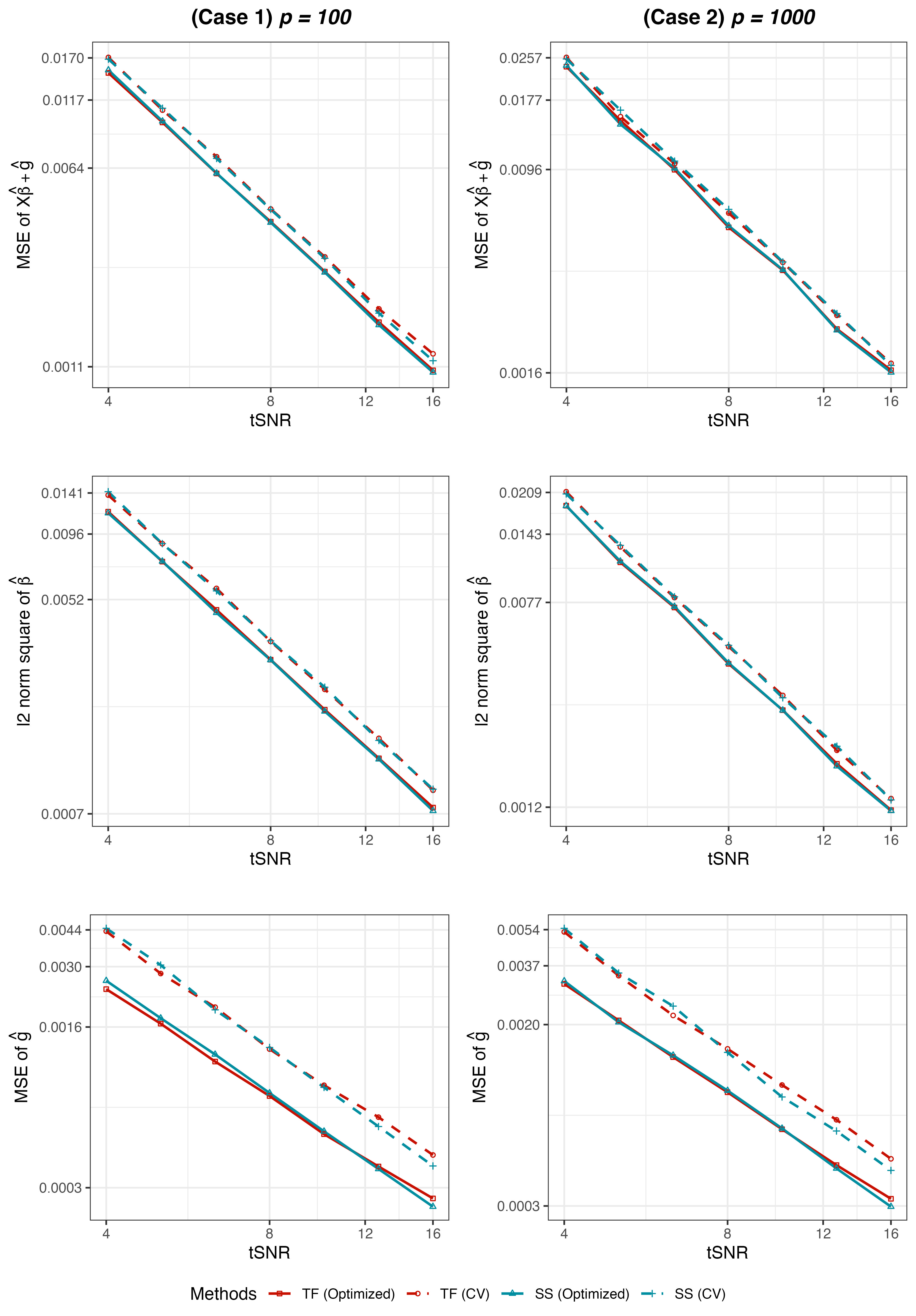
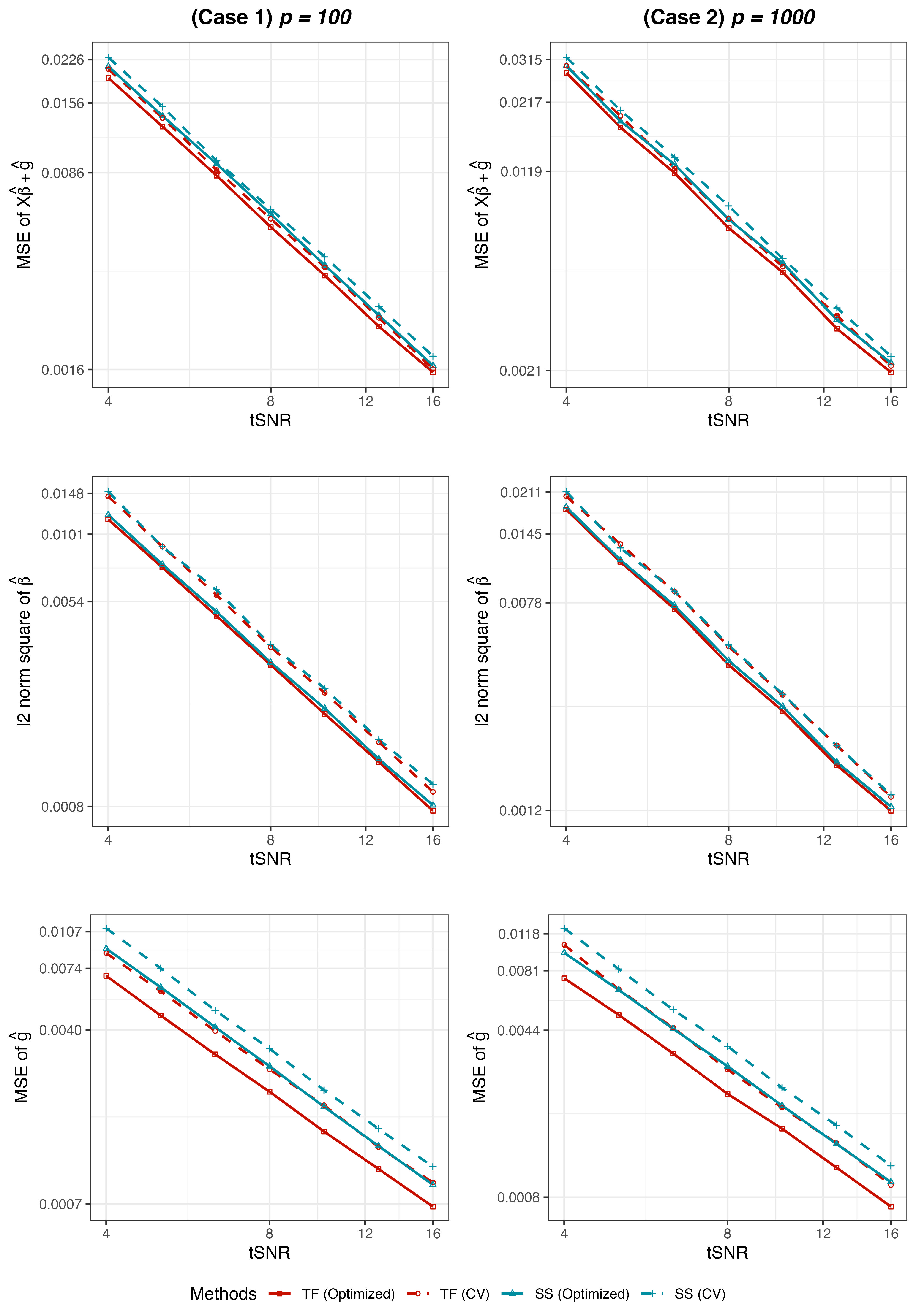
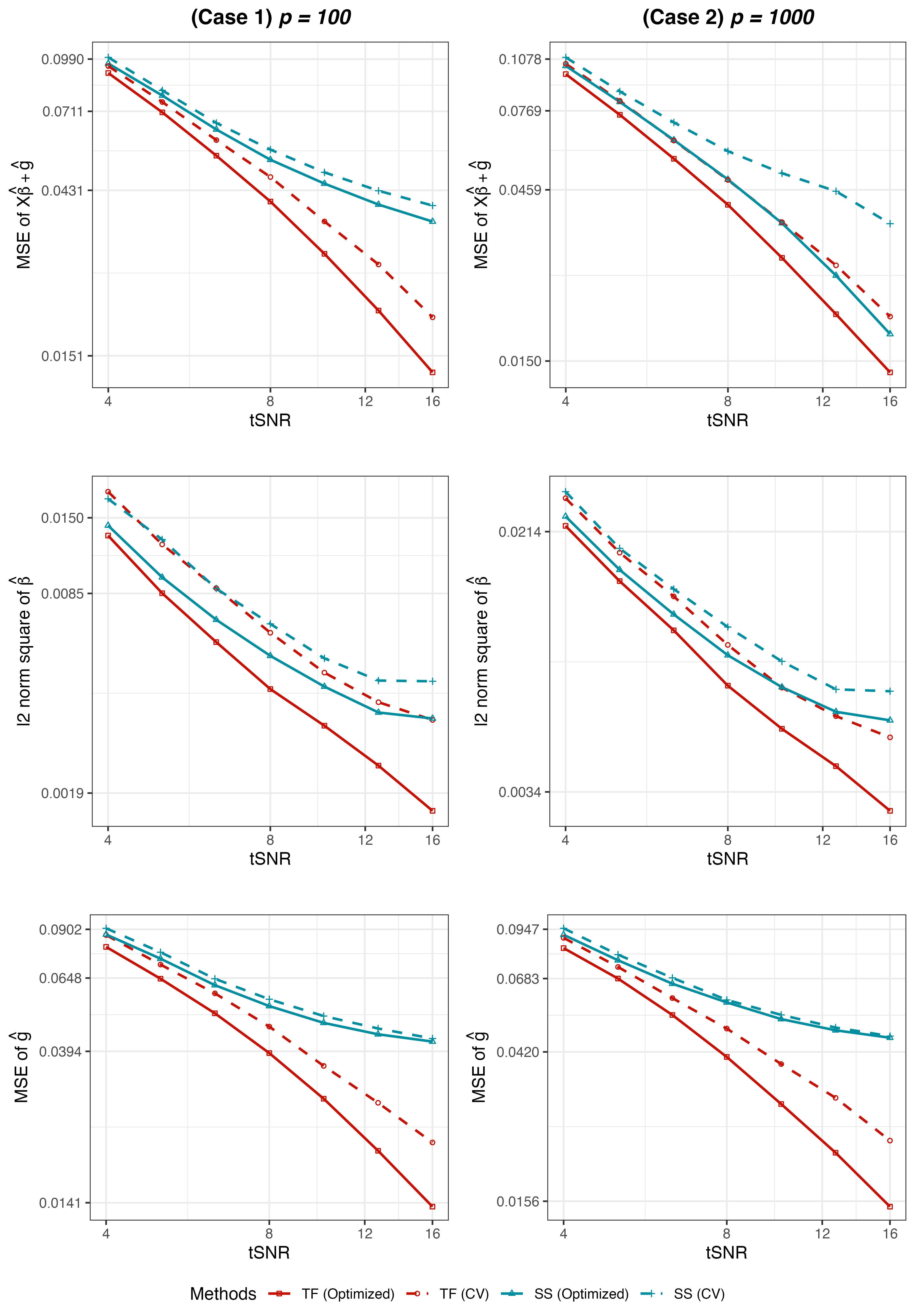
The simulation results are displayed in Figures 3-5. Figure 3 demonstrates that when the function has spatially homogeneous smoothness, the performance of the PLTF method is comparable to that of the PLSS method, with no significant differences observed. However, as shown in Figure 4, when the function exhibits variable spatial smoothness, the difference between the two methods becomes more pronounced. PLTF starts to outperform PLSS, especially for the estimation of . When the degree of heterogeneous smoothness of increases further, as seen in Figure 5, all the three errors of PLTF are significantly lower than those of PLSS in both low and high-dimensional cases. This disparity becomes more apparent as the tSNR increases. These simulation results suggest that for functions with homogeneous smoothness, PLTF and PLSS are competitive. However, as the function becomes more heterogeneously smooth, PLTF can significantly outperform PLSS in both low and high-dimensional scenarios, particularly when the tSNR is high. The empirical findings are aligned with those for comparing trend filtering and smoothing splines in the context of univariate nonparametric regressions and additive regression models (Tibshirani, 2014; Sadhanala and Tibshirani, 2019).
4 Real data analyses with IDATA Study
4.1 Interactive Diet and Activity Tracking in AARP (IDATA) Study
The Interactive Diet and Activity Tracking in AARP (IDATA) Study was specifically designed to evaluate the efficacy of web-based dietary assessment tools, including the Automated Self-Administered 24-hour Dietary Assessment Tool (ASA-24), four-day food records (4DFRs), and the Dietary History Questionnaire (DHQ) II, in comparison to reference biomarkers (Subar et al., 2020). Briefly, participants were recruited from a cohort of AARP members aged 50-74 years, residing in or near Pittsburgh, Pennsylvania, who met the following inclusion criteria: English-speaking, internet access, not currently engaged in a weight-loss diet, a body mass index (BMI) below 40 kg/m2, and no significant medical conditions or mobility limitations. Between 2012 and 2013, 1,082 participants were enrolled in the study, all of whom provided consent for biospecimen collection (Park et al., 2018). The study protocol was approved by the NCI Special Studies Institutional Review Board and registered on ClinicalTrials.gov (Identifier: NCT03268577). All participants provided written informed consent (Subar et al., 2020). Additional details on the design and methodology of the IDATA study have been thoroughly outlined on https://cdas.cancer.gov/idata/.
4.2 Dietary data and biological sample collections
Participants were divided into four groups to minimize the impact of seasonal variations in diet and for practical reasons related to study centers. Over a 12-month period, participants completed up to six web-based ASA-24 assessments, administered on randomly assigned days approximately every two months (Park et al., 2018). Each reported food and beverage item was assigned a unique 8-digit food code based on the ”What We Eat in America” (WWEIA) database (Martin et al., 2014), as part of NHANES (Steele et al., 2023). These codes were linked to the Food and Nutrient Database for Dietary Studies (FNDDS) (Martin et al., 2014), which is used to convert food and beverage portions into gram amounts and estimate nutrient values, including energy, by employing standard reference codes (SR codes) from the USDA National Nutrient Database for Standard Reference.
The intake of ultra-processed foods (UPF) was estimated using the Nova system, which categorizes foods and beverages into four groups according to the degree and purpose of industrial processing. Group 1 includes unprocessed or minimally processed foods, such as fresh, dried, or frozen fruits and vegetables, grains, legumes, meat, fish, and milk. In contrast, Group 4 comprises UPFs, such as ready-to-eat products like commercially prepared breads and baked goods, which contain ingredients not commonly used in traditional culinary practices. We disaggregated each FNDDS food code into its corresponding SR codes through a series of merges. Each IDATA food item (identified by food code and SR code) was then assigned to one of the four Nova groups and one of 37 mutually exclusive food subgroups, as specified by the WWEIA, NHANES database developed by Steele et al. (2019, 2023). For FNDDS food codes that had not yet been classified into a Nova group or subgroup, a manual review was conducted, and the classification was determined using the ”reference approach” outlined by (Steele et al., 2023).
The total daily intake, in grams, was calculated for each of the four main Nova groups (Groups 1 to 4, ranging from unprocessed to highly processed). For ASA-24, we averaged the proportion of total energy derived from UPF across multiple days. Further details regarding the calculation of UPF intake using the Nova system can be found in Steele et al. (2019, 2023).
For the metabolomics datasets, participants visited the study center at months 1, 6, and 12 to have anthropometric measurements taken. During two of these visits—either at months 1 and 6 or at months 6 and 12—blood (serum) samples were collected. Participants were also instructed to perform urine collection at home, which was scheduled approximately 7 to 10 days after a study center visit. They were asked to collect 100 mL of their first-morning void (FMV).
Serum and urine metabolomic analyses were conducted by Metabolon Inc. using ultra-high-performance liquid chromatography (UPLC) coupled with tandem mass spectrometry (MS/MS) to measure a wide range of metabolites. These included endogenously derived amino acids, carbohydrates, lipids, cofactors and vitamins, energy metabolism intermediates, as well as xenobiotics originating from external sources like food or drugs. Serum and urine were analyzed separately, and all samples were prepared using the automated MicroLab STAR system (Hamilton Company). Metabolite values below the detection limit were assigned the minimum observed value for each metabolite and were standardized. For analysis, metabolite levels were log-transformed.
4.3 Data analyses and results
In order to investigate the relationship between metabolomic profiles and ultra-processed food (UPF) intake, we set the response variable as the UPF intake and the metabolite concentrations as the covariates . Specifically, we consider 970 metabolites () from the serum dataset and 1018 metabolites () from the urine dataset. After conducting the preprocessing steps outlined earlier, the final dataset comprises 718 observations (). This dataset forms the basis for subsequent analyses aimed at identifying potential associations between metabolite levels and UPF consumption.
Recent studies (Juul et al., 2018; Sung et al., 2021) have highlighted sexual differences in UPF intake between females and males. Motivated by these findings, we aim to further explore the heterogeneous effects of these variables by generating two subgroups based on sex. The two categories considered are female () and male (). Additionally, previous research has shown that certain obesity-related body measurements (Canhada et al., 2020) and age (Fu et al., 2024b) exhibit significant nonlinear relationships with UPF intake. Therefore, we include age, BMI, waist circumference, and hip circumference as covariates () and model them flexibly, without assuming linearity, by applying trend filtering.
We present two main types of results from the analyses: (1) prediction accuracy and (2) selected variables. For prediction accuracy, we compare three distinct methods: PLTF, PLSS, and LASSO. In the case of LASSO, is initially fixed as a selected covariate. Consistent with our simulation settings, we set for PLTF and for PLSS, to regularize the second derivative of . To evaluate prediction performance, we randomly divide the dataset, using 90% for training and 10% for testing. Models are trained on the training dataset using 10-fold cross-validation (CV), and the mean squared error (MSE) is computed on the testing set. This procedure is repeated 500 times, with the number of repetitions chosen to ensure standard errors are within 1% to 2% of the MSE. The prediction errors are reported in Table 1. The prediction results indicate that, in the majority of cases, PLTF outperformed the other models (12 out of 16 cases). Notably, for the serum datasets, PLTF significantly outperformed the other methods, particularly in the female subgroup. In the urine datasets, PLTF generally demonstrated better performance. Even in cases where other models marginally outperformed PLTF, the difference between PLTF and the best-performing model was not statistically significant.
| Age | BMI | Hip | Waist | |||
|---|---|---|---|---|---|---|
| Serum | Female | PLTF | 175.390 (2.289) | 174.789 (2.328) | 176.591 (2.312) | 177.725 (2.360) |
| PLSS | 178.696 (2.383) | 180.286 (2.420) | 180.230 (2.390) | 180.331 (2.440) | ||
| LASSO | 188.370 (2.516) | 190.647 (2.555) | 190.461 (2.545) | 190.115 (2.543) | ||
| Male | PLTF | 152.774 (2.012) | 150.925 (1.994) | 153.823 (1.991) | 154.350 (2.055) | |
| PLSS | 152.904 (2.019) | 154.373 (2.019) | 153.470 (1.996) | 155.080 (2.070) | ||
| LASSO | 155.738 (2.036) | 156.044 (2.045) | 156.342 (2.040) | 156.619 (2.062) | ||
| Urine | Female | PLTF | 171.911 (2.361) | 169.977 (2.371) | 170.057 (2.350) | 172.937 (2.469) |
| PLSS | 172.365 (2.425) | 171.910 (2.427) | 171.859 (2.421) | 172.696 (2.473) | ||
| LASSO | 172.343 (2.468) | 172.626 (2.494) | 173.094 (2.488) | 172.584 (2.483) | ||
| Male | PLTF | 144.786 (1.894) | 143.859 (1.905) | 145.162 (1.868) | 144.145 (1.920) | |
| PLSS | 144.299 (1.894) | 144.790 (1.877) | 145.145 (1.856) | 144.803 (1.904) | ||
| LASSO | 148.020 (1.996) | 147.060 (1.997) | 147.009 (1.982) | 146.509 (2.017) |
Regarding variable selection, due to the diversity of datasets, we report the top 10 selected variables from each dataset. These variables are ranked based on the absolute magnitude of their coefficients. To ensure fair comparisons across coefficients, all covariates are standardized. The full list of the top 10 selected variables is provided in Table S1 and Table S2 of the supplementary material. Rather than listing all selected variables, we focus on those that were selected multiple times across different types of . These results are summarized in Table 2. The selected variables differ across datasets, with their super pathways and biological functions also varying. For example, Saccharin, which was selected in the male serum dataset and the female urine dataset, is a well-known artificial sweetener commonly found in UPF products. Given that the signs of the coefficients are positive, this aligns with expected findings. Quinate, selected in both the male serum and urine datasets, is commonly present in foods such as coffee. This suggests that coffee consumption in the male population may have an indirect negative association with UPF intake, as reflected by the negative coefficient.
| Selected Variables | |||
| Biochemical | Super Pathway | ||
| Serum | Female | Diglycerol (+) | Xenobiotics |
| 4-Allylphenol sulfate (-) | Xenobiotics | ||
| Anthranilate (+) | Amino Acid | ||
| Eicosapentaenoylcholine (-) | Lipid | ||
| 1-Stearoyl-2-Adrenoyl-GPC | Lipid | ||
| (18:0/22:4) (+) | |||
| Branched chain 14:0 dicarboxylic acid (-) | Lipid | ||
| X-21807 (-) | Unknown | ||
| X-25523 (-) | Unknown | ||
| Male | Quinate (-) | Xenobiotics | |
| Saccharin (+) | Xenobiotics | ||
| 1-Methylhistidine (+) | Amino Acid | ||
| 1-(1-Enyl-palmitoyl)-2-Oleoyl-GPE | Lipid | ||
| (P-16:0/18:1) (-) | |||
| 1-Lignoceroyl-GPC (24:0) (-) | Lipid | ||
| X-19183 (-) | Unknown | ||
| X-21442 (-) | Unknown | ||
| X-23655 (-) | Unknown | ||
| Urine | Female | Galactonate (-) | Carbohydrate |
| Riboflavin (vitamin B2) (-) | Cofactors and Vitamins | ||
| Saccharin (+) | Xenobiotics | ||
| 2,3-Dihydroxypyridine (-) | Xenobiotics | ||
| Glutamine conjugate of C8H12O2 (3) (-) | Partially Characterized Molecules | ||
| X-12096 (+) | Unknown | ||
| X-12753 (-) | Unknown | ||
| X-23680 (+) | Unknown | ||
| X-25936 (+) | Unknown | ||
| X-25952 (+) | Unknown | ||
| Male | Quinate (-) | Xenobiotics | |
| 1,6-Anhydroglucose (+) | Xenobiotics | ||
| N-Acetylcitrulline (+) | Amino Acid | ||
| 3-Methoxytyramine (+) | Amino Acid | ||
| Cortisone (-) | Lipid | ||
| Ursocholate (+) | Lipid | ||
| X-13847 (-) | Unknown | ||
| X-23161 (-) | Unknown | ||
| X-25952 (+) | Unknown | ||
Several other findings, including the direction of the coefficients, are consistent with existing research on UPF intake. For instance, 4-Allylphenol sulfate has been identified as a potential biomarker for UPF intake (O’Connor et al., 2023). Diglycerol can be found in cosmetics or can be esterified to Aiglycerol esters of fatty acids. Aiglycerol esters of fatty acids is a well-known emulsifier used in UPFs, and the effects of emulsifiers in UPFs and their positive association with various cancer risks have been explored in Sellem et al. (2024).
Additionally, Eicosapentaenoylcholine is known to be highly positively correlated with Vitamin D consumption (Leung et al., 2020), and previous studies have shown that UPF intake negatively impacts dietary Vitamin D (Falcão et al., 2019). Vitamin B2 deficiency related to UPF intake in women, along with its potential impact on pregnancy, has been studied in Schenkelaars et al. (2024). Lastly, a positive association of 1,6-Anhydroglucose with UPF intake has been identified in urine datasets (Muli et al., 2024). Several other findings involve metabolites that have not been extensively studied or are unknown. These may represent potential novel biomarkers associated with UPF intake, providing new insights for future research.
5 Discussion
In this paper, we expanded the framework of trend filtering to high-dimensional partial linear models. Using doubly penalized least square estimation, our approach preserves the local adaptivity and computational efficiency of univariate trend filtering. We studied its degrees of freedom and established the optimal convergence rates. We further demonstrated through empirical examples that the proposed method outperforms a standard smoothing spline based method when the underlying functions possess variable spatial smoothness.
There are several important directions for future research:
-
•
When the covariate has dimension , we can extend our work by considering an additive function form where for some constant . The penalty in (5) is then replaced with . Leveraging computational and theoretical treatment in additive trend filtering (Sadhanala and Tibshirani, 2019), our method and theory can be readily generalized to the setting when is bounded. For the high-dimensional case where is comparable to or much larger than , a natural extension is to consider a sparse additive form for and employ an additional sparsity-induced penalty (e.g. empirical norm) for each function . The theoretical development is much more challenging, however, recent results in high-dimensional additive trend filtering (Tan and Zhang, 2019) might be helpful in the context of partial linear models.
-
•
A key question in partial linear models is how to decide which covariates are linear and which are nonlinear. In the paper, we have assumed this model structure is known. However, such prior knowledge is not necessarily available in practice. Some successful penalization based approaches have been developed for the structure selection, assuming the underlying functions belong to Sobolev or Holder classes (Zhang et al., 2011; Huang et al., 2012; Lian et al., 2015). It would be interesting to investigate how trend filtering can be adapted for the model structure discovery in the presence of more heterogeneously smooth functions.
-
•
Under partial linear models, variable selection and statistical inference for the linear part can be important tasks. It would be particularly valuable to study how recent advances in high-dimensional linear regression models (Zhang and Zhang, 2014; van de Geer et al., 2014; Javanmard and Montanari, 2014; Dezeure et al., 2015; Barber and Candès, 2015; Candes et al., 2018; Dai et al., 2023) can be extended to high-dimensional partial linear trend filtering, in order to perform variable selection and inference with guaranteed error control.
.
6 Proofs
6.1 Proof of Proposition 1
We first cite Theorem 3 from Tibshirani and Taylor (2012) on the generalized lasso degrees of freedom.
Theorem 3 (Tibshirani and Taylor (2012)).
Consider the generalized lasso problem,
| (13) |
where and . Define the active set . Assuming , for any and , the degrees of freedom of is
The proof of Part (i) is a direct application of the above theorem. Denote
Then, (9) can be rewritten in the form of (13). Thus we can invoke Theorem 3 and obtain
where denotes the vector after removing components indexed by . As a result,
Regarding Part (ii), the proof is motivated by that of Lemma 3 in Sadhanala and Tibshirani (2019). We use the equivalent formulation (8) to derive the degrees of freedom. We have
| (14) |
where . The problem (6.1) is a standard lasso problem,
| (15) |
where and . Let be the projection operator onto the column space where has orthonormal columns, and . Then the equivalence among (8), (9), (6.1) and (15) yields
Therefore,
Note that above is the degrees of freedom of the standard lasso (15) under the model . Since has columns in general position, the lasso solution is unique (Tibshirani, 2013). As a result,
where in the last step we have used and the expression for from Wang et al. (2014).
6.2 Proof of Theorem 1
Throughout the proof, we use to denote universal constants and use to denote constants that may only depend on the constants from Conditions 1-5. An explicit (though not optimal) dependence of on the aforementioned constants can be tracked down. However, since it does not provide much more insight, we will often not present the explicit forms of , and this will greatly help streamline the proofs. The constants may vary from lines to lines.
6.2.1 Roadmap of the proof
For a given function with , introduce the functional
| (16) |
where for notational simplicity we have suppressed the dependence of on the tuning parameters . This functional will serve as a critical measure for and . Define the following events:
The general proof idea is largely inspired by Müller and Van de Geer (2015) (see also Yu et al. (2019)). We first use a localization technique based on convexity to show that under the event , the bound on in Theorem 1 (bound on is derived similarly) holds. This is done in Lemmas 1-2. Then in Lemmas 3 and 4 we show that the event happens with high probability. Along the way we need to choose in (16) properly to meet conditions in Lemmas 1-4 and to achieve the desirable error rate in Theorem 1. We complete this step in Section 6.2.3.
6.2.2 Important lemmas
Lemma 1.
Assuming Condition 4 and , then on , there exists such that
-
(i)
, where are constants only dependent on .
-
(ii)
.
Proof.
According to Lemma 16 in Tibshirani (2022) (see also Lemma 13 in Sadhanala and Tibshirani (2019)), there exists such that result (i) holds on . We use such a in the rest of the proof. Consider the convex combination
Accordingly, define
For the choice of , it is straightforward to verify that
| (17) |
Hence, to prove result (ii) it is sufficient to show . We start with the basic inequality due to the convex problem (5),
which can be simplified to
Using the triangle inequality for and , we can continue from the above to obtain
| (18) |
Observing from (17) that belongs to the set , on we can proceed with
| (19) |
where the third inequality holds due to (6.2.2), and in the last inequality we have used result (i) and Cauchy-Schwarz inequality for . Now Condition 4 implies that
Here, the second inequality follows , and the third inequality is due to the orthogonal decomposition . This together with (19) yields
where the last inequality holds under the assumed condition on (with proper choice of constant ). The above bound further implies since , and , leading to the bound . ∎
Lemma 2.
Under the same conditions of Lemma 1, then on , it holds that
Moreover, define a subevent of :
with . Then on , it holds that
Proof.
Part (ii) in Lemma 1 together with Part (i) of Lemma 5 implies that . As a result, combining it with Part (i) of Lemma 1 gives
To prove the second result, we first use results (i)(ii) of Lemma 1 to bound
Combining the above with the first result on , we see that
Hence, on , we can use the bound on to obtain the bound on :
∎
Lemma 3.
Proof.
For a given function , it is clear that
such that
We now bound the above three terms separately. According to Lemma 5 Part (i), the in any with satisfies
| (21) |
Therefore,
| (22) |
where in the last inequality we have used the fact . Condition 1 implies that are independent, zero-mean, sub-exponential random variables with the sub-exponential norm . We then use Bernstein’s inequality in Theorem 4 together with a simple union bound to obtain that when ,
holds with probability at least . Putting this result together with (22) enables us to conclude , as long as .
Now we bound . Using Lemma 5 we have , where
| (23) | |||
We aim to apply Theorem 6 to bound . Adopting the notation in Theorem 6, we first calculate :
| (24) |
where the first inequality is due to the entropy bound of Corollary 1 in Sadhanala and Tibshirani (2019). As a result,
We are ready to invoke Theorem 6. The condition is reduced to
| (25) |
and under this condition it holds with probability at least that
Given the above, choosing and assuming a slightly stronger condition compared to (25), it is then straightforward to verify that .
Next we bound . We first use Hölder’s inequality and Lemma 5 to obtain
We then aim to use Theorem 7 to bound for each . The quantities in Theorem 7 become . Let , and be a Rademacher sequence independent of . Applying Dudley’s entropy integral gives
| (26) |
where is from (24) and the second to last inequality is due to (24); denotes the weighted empirical norm and it is clear that and . Now applying the second result in Theorem 7 yields
| (27) |
Define the events
Condition 1 together with standard union bound for sub-Gaussian tails gives (with a proper choice of ). The previous result on term shows , and it holds on that
| (28) |
As a result, we can further bound (27) on to arrive at
We integrate out the above conditional probability to obtain the unconditional one:
It is then direct to verify that choosing gives
| (29) |
We will invoke the symmetrization result of Theorem 7 to transfer the above bound to . In order to do so, we need to show . Note that
Using the sub-Gaussian tail bound for to bound , it is not hard to obtain that with the choice . Therefore, under the condition , Theorem 7 together with (29) leads to
We follow via a union bound,
Finally, we collect the results on to bound via .
Regarding the bound for , first note that under the assumption . Moreover, . Hence,
Essentially, all the previous arguments in bounding carry over into , up to constants ’s. We only need to update those constants in the conditions and results, in a way so that and share the same constants (e.g., taking a minimum or maximum among constants). ∎
Lemma 4.
Proof.
Recalling the sets in (21) and in (23) from the proof of Lemma 3, we have
We first bound term . Using Bernstein’s inequality in Theorem 4 we obtain that . This combined with a union bound gives
To bound term , let . Conditional on (which are independent from ), Theorem 8 implies that the following holds with probability at least :
where the last inequality follows as in (26). Integrating over , the above holds marginally with probability at least as well. Moreover, from (28) we already know that,
Combining these two results via a union bound gives us
Choosing and assuming , it is direct to confirm
Combining the bounds for gives the bound for
Finally, the bound on is directly taken from Lemma 5 in Wang et al. (2014). ∎
Lemma 5.
Proof.
The bound on and is clear from the definition of in (16). Using the orthogonal decomposition:
we have , and
Having the bound on , we can further obtain .
It remains to bound . Define , then due to the derived bounds on and . Hence it is sufficient to show that
To prove the above, we first decompose , where is a polynomial of degree and is orthogonal to all polynomials of degree (with respect to the inner product ). Note that . Then Lemma 5 in Sadhanala and Tibshirani (2019) implies that for a constant only depending on . Now write . We have
where and with . Thus, we obtain
which implies . Finally, we need to show is bounded below by a constant only depending on and . Under Condition 3 we have
where is the minimizer; is a constant only depending on , and it is positive because the roots of any polynomial (not identically zero) form a set of Lebesgue measure zero.
∎
6.2.3 Completion of the proof
We are in the position to complete the proof of Theorem 1. In fact, we shall prove Theorems 1 and 2 altogether. We will choose such that the conditions in Lemmas 1-4 (for Theorem 1) and Lemmas 6-7 (for Theorem 2) are all satisfied. As a result, we will then conclude that the bounds on in Lemma 2 and bounds on in Lemma 6 hold with probability at least . Towards this end, we first list the conditions to meet555With a bit abuse of notation, the subscripts for constants ’s we use here may be different from the ones in the lemmas.:
- (i)
- (ii)
-
(iii)
Conditions from Lemma 4: , .
-
(iv)
Conditions from Lemma 6: .
-
(v)
Conditions from Lemma 7: , , .
We choose , where is any given constant that may only depend on . It remains to specify . We will consider , which together with implies
Define
For any , it is straightforward to verify that Conditions from Lemmas 1-2 and all the conditions involving are satisfied. To meet other conditions, we will pick for any constant . We verify the remaining conditions by showing that under the scaling as (so that ):
-
(ii)
Conditions from Lemma 3: . Moreover, when ; when , it still holds that
-
(iii)
Conditions from Lemma 4: .
-
(iv)
Conditions from Lemma 6: .
- (v)
Finally, given what we have obtained, it is straightforward to further evaluate the high probability (by choosing the constant in and in large enough):
when is large enough under the scaling .
6.3 Proof of Theorem 2
6.3.1 Roadmap of the proof
Recall the sets in (21) and in (23) from the proof of Lemma 3. Define the following set and events:
The proof of Theorem 1 already yields an error rate for (see Lemmas 1 and 5), however, the rate is not optimal yet. We will base on this “slow rate” result to perform a finer analysis of to obtain the “fast rate”. This is again inspired by Müller and Van de Geer (2015). Specifically, we prove in Lemma 6 that the “fast rate” results on in Theorem 2 hold by intersecting with another event . We then show in Lemma 7 that this additional event also has large probability.
6.3.2 Important lemmas
Lemma 6.
Proof.
Recall that under Condition 5, where . According to Lemma 16 in Tibshirani (2022), there exist for all such that
where are constants only depending on , and is the span of the th degree falling factorial basis functions with knots . Define
Note that since . Therefore, we can write down a basic inequality,
which can be reformulated as
Using triangle inequality for and Hölder’s inequality, we can proceed to obtain
| (30) |
To further simplify the above inequality, we observe the following:
-
(i)
on
- (ii)
Based on these two results and assuming , we continue from (30) to achieve that on ,
A standard argument in the literature of Lasso (e.g., Lemma 6.3 in Bühlmann and Van De Geer (2011)) simplifies the above to
where the second to last equality is due to , and the last inequality holds on . Rearranging the terms leads to
| (31) |
Now (31) combined with the condition from implies
Further intersecting with , we obtain
∎
Lemma 7.
Proof.
For with ,
Using Hoeffding’s inequality in Theorem 4, we obtain666Given that , it holds that .
Thus with probability at least ,
| (35) |
Next we have
Note that we have used Bernstein’s inequality to bound in the proof of Lemma 4. The same result holds here,
Since are independent, zero-mean, sub-exponential random variables with , we use again Bernstein’s inequality to obtain
Hence with probability at least ,
| (36) |
We continue in the following way,
| (37) |
As in bounding earlier, we bound
Moreover, applying the same arguments for bounding in the proof of Lemma 3, we have that under the conditions (32)-(33),
| (38) |
Regarding the bound for and , the proof follows the same arguments used for bounding term in the proof of Lemma 3. ∎
6.3.3 Completion of the proof
See Section 6.2.3.
6.4 Proof of Proposition 1
From previous results, we know that (9) is the same as (5). We use the notation from (9). For given and fixed , the objective of minimization in (9) can be rewritten as below
where and be block diagonal matrix with entries and . Then minimization with respect to is a generalized lasso problem now. We denote be the generalized lasso estimator of . By applying Theorem 3 from Tibshirani and Taylor (2012), we have
where , and denotes the matrix with rows removed that correspond to the set . Followed by the results of Theorem 2 from Tibshirani and Taylor (2012) and Section 1.1 from Tibshirani (2014) we have
where is a cardinality. Therefore, we finish the proof.
6.5 Reference materials
Theorem 4.
(General Hoeffding’s inequality). Let be independent, zero-mean, sub-gaussian random variables. Then for every , we have
where is an absolute constant, and is the sub-gaussian norm defined as .
(Bernstein’s inequality). Let be independent, zero-mean, sub-exponential random variables. Then for every , we have
where is an absolute constant, and is the sub-exponential norm defined as .
The above two results are Theorem 2.6.2 and Theorem 2.8.1, respectively in Vershynin (2018).
Theorem 5.
Let be sub-gaussian random variables, which are not necessarily independent. Then there exists an absolute constant such that for all ,
The above result can be found in Lemma 2.4 of Boucheron et al. (2013).
Theorem 6.
(Uniform convergence of empirical norms). Denote for i.i.d. samples . For a class of functions on , let , where is some universal constant and is the metric entropy. Let , and be the convex conjugate of . Then, for all and all ,
where is a universal constant.
The above is Theorem 2.2 from van de Geer (2014).
Theorem 7.
(Symmetrization and concentration). Let be i.i.d. samples in some sample space and let be a class of real-valued functions on . Define . Then,
where is a Rademacher sequence independent of and is a universal constant.
The first result is Lemma 16.1 in Van de Geer (2016) and the second result is implied by Theorem 16.4 in Van de Geer (2016).
Theorem 8.
(Dudley’s integral tail bound). Let be a separable random process on a metric space with sub-Gaussian increments: . Then, for every , the event
holds with probability at least . Here, is a universal constant, is the metric entropy, and .
The result above is Theorem 8.1.6 in Vershynin (2018).
7 Supplementary tables
We present the full top 10 selected variables for both serum and urine datasets here.
| Selected Variables | ||
|---|---|---|
| Female | Age | diglycerol, 21807, |
| 1-stearoyl-2-adrenoyl-gpc–18, anthranilate, | ||
| 4-allylphenol-sulfate, 25523, | ||
| n-acetylglucosamine-n-acetylga, eicosapentaenoylcholine, | ||
| fibrinopeptide-a–3-15—, 17145 | ||
| BMI | 21807, quinate, | |
| eicosapentaenoylcholine, diglycerol, | ||
| 25523, 2s-3r-dihydroxybutyrate, | ||
| 2-3-dihydroxyisovalerate, fibrinopeptide-a–3-15—, | ||
| 4-allylphenol-sulfate, 2–deoxyuridine | ||
| Hip | diglycerol, 21807, | |
| quinate, eicosapentaenoylcholine, | ||
| 25523, 1-stearoyl-2-adrenoyl-gpc–18, | ||
| 4-allylphenol-sulfate, 17145, | ||
| anthranilate, 1-methylurate | ||
| Waist | diglycerol, 1-stearoyl-2-adrenoyl-gpc–18, | |
| 21807, 25523, | ||
| anthranilate, 4-allylphenol-sulfate, | ||
| eicosapentaenoylcholine, glutamine, | ||
| 17145, pentose-acid- | ||
| Male | Age | 21442, 23655, |
| 1-methylhistidine, quinate, | ||
| 1-lignoceroyl-gpc–24-0-, 19183, | ||
| 1–1-enyl-palmitoyl–2-o-gpe, saccharin, | ||
| 23585, orotidine | ||
| BMI | 21442, 23655, | |
| 1-methylhistidine, quinate, | ||
| decadienedioic-acid–c10-2-dc, 19183, | ||
| 1-lignoceroyl-gpc–24-0-, 23585, | ||
| saccharin, 1–1-enyl-palmitoyl–2-o-gpe | ||
| Hip | 21442, 23655, | |
| quinate, 1-methylhistidine, | ||
| n-delta-acetylornithine, 17145, | ||
| 1-lignoceroyl-gpc–24-0-, xanthurenate, | ||
| 19183, 1–1-enyl-palmitoyl–2-o-gpe | ||
| Waist | 21442, 23655, | |
| quinate, 1-methylhistidine, | ||
| 1-lignoceroyl-gpc–24-0-, 19183, | ||
| n-delta-acetylornithine, saccharin, | ||
| 17145, xanthurenate |
| Selected Variables | ||
|---|---|---|
| Female | Age | 999925952, 12096, |
| saccharin, 2-3-dihydroxypyridine, | ||
| 23680, galactonate, | ||
| 100020267, 12753, | ||
| sucrose, 25936 | ||
| BMI | 999925952, 12096, | |
| saccharin, 2-3-dihydroxypyridine, | ||
| galactonate, 100020267, | ||
| 23680, riboflavin–vitamin-b2-, | ||
| 12753, 24352 | ||
| Hip | 999925952, 12096, | |
| 2-3-dihydroxypyridine, saccharin, | ||
| galactonate, 100020267, | ||
| 23680, 24352, | ||
| riboflavin–vitamin-b2-, 25936 | ||
| Waist | 999925952, 12096, | |
| saccharin, 2-3-dihydroxypyridine, | ||
| galactonate, 100020267, | ||
| 23680, riboflavin–vitamin-b2-, | ||
| 25936, 12753 | ||
| Male | Age | 999925952, 999923161, |
| quinate, 1-6-anhydroglucose, | ||
| 3-methoxytyramine, cortisone, | ||
| x5-aminolevulinic-aci, 999913847, | ||
| n-acetylcitrulline, 21807 | ||
| BMI | 999925952, 999923161, | |
| quinate, 999913847, | ||
| 3-methoxytyramine, 1-6-anhydroglucose, | ||
| cortisone, n-acetylcitrulline, | ||
| n6-succinyladenosine, ursocholate | ||
| Hip | 999923161, 999925952, | |
| quinate, 999913847, | ||
| 3-methoxytyramine, n-acetylcitrulline, | ||
| 1-6-anhydroglucose, cortisone, | ||
| ursocholate, thioproline | ||
| Waist | 999923161, 999925952, | |
| quinate, 999913847, | ||
| 3-methoxytyramine, 1-6-anhydroglucose, | ||
| thioproline, ursocholate, | ||
| n-acetylcitrulline, cortisone |
References
- Arnold et al. (2014) Arnold, T., Sadhanala, V. and Tibshirani, R. (2014). glmgen: Fast algorithms for generalized lasso problems. R package version 0.0.3.
- Barber and Candès (2015) Barber, R. F. and Candès, E. J. (2015). Controlling the false discovery rate via knockoffs. The Annals of statistics 2055–2085.
- Boucheron et al. (2013) Boucheron, S., Lugosi, G. and Massart, P. (2013). Concentration Inequalities: A Nonasymptotic Theory of Independence. Oxford University Press.
- Bühlmann and Van De Geer (2011) Bühlmann, P. and Van De Geer, S. (2011). Statistics for high-dimensional data: methods, theory and applications. Springer Science & Business Media.
- Bunea (2004) Bunea, F. (2004). Consistent covariate selection and post model selection inference in semiparametric regression. Ann. Statist., 32 898–927.
- Candes et al. (2018) Candes, E., Fan, Y., Janson, L. and Lv, J. (2018). Panning for gold:‘model-x’knockoffs for high dimensional controlled variable selection. Journal of the Royal Statistical Society Series B: Statistical Methodology, 80 551–577.
- Canhada et al. (2020) Canhada, S. L., Luft, V. C., Giatti, L., Duncan, B. B., Chor, D., Maria de Jesus, M., Matos, S. M. A., Molina, M. d. C. B., Barreto, S. M., Levy, R. B. et al. (2020). Ultra-processed foods, incident overweight and obesity, and longitudinal changes in weight and waist circumference: the brazilian longitudinal study of adult health (elsa-brasil). Public health nutrition, 23 1076–1086.
- Chen (1988) Chen, H. (1988). Convergence rates for parametric components in a partly linear model. The Annals of Statistics 136–146.
- Dai et al. (2023) Dai, C., Lin, B., Xing, X. and Liu, J. S. (2023). False discovery rate control via data splitting. Journal of the American Statistical Association, 118 2503–2520.
- Dezeure et al. (2015) Dezeure, R., Bühlmann, P., Meier, L. and Meinshausen, N. (2015). High-dimensional inference: confidence intervals, p-values and r-software hdi. Statistical science 533–558.
- Donoho and Johnstone (1998) Donoho, D. L. and Johnstone, I. M. (1998). Minimax estimation via wavelet shrinkage. The annals of Statistics, 26 879–921.
- Engle et al. (1986) Engle, R. F., Granger, C. W., Rice, J. and Weiss, A. (1986). Semiparametric estimates of the relation between weather and electricity sales. Journal of the American statistical Association, 81 310–320.
- Falcão et al. (2019) Falcão, R. C. T. M. d. A., Lyra, C. d. O., Morais, C. M. M. d., Pinheiro, L. G. B., Pedrosa, L. F. C., Lima, S. C. V. C. and Sena-Evangelista, K. C. M. (2019). Processed and ultra-processed foods are associated with high prevalence of inadequate selenium intake and low prevalence of vitamin b1 and zinc inadequacy in adolescents from public schools in an urban area of northeastern brazil. PLoS One, 14 e0224984.
- Fan and Li (2001) Fan, J. and Li, R. (2001). Variable selection via nonconcave penalized likelihood and its oracle properties. Journal of the American statistical Association, 96 1348–1360.
- Friedman et al. (2010) Friedman, J., Hastie, T. and Tibshirani, R. (2010). Regularization paths for generalized linear models via coordinate descent. Journal of Statistical Software, 33 1–22.
- Fu et al. (2024a) Fu, X., Huang, M. and Yao, W. (2024a). Semiparametric efficient estimation in high-dimensional partial linear regression models. Scandinavian Journal of Statistics.
- Fu et al. (2024b) Fu, Y., Chen, W. and Liu, Y. (2024b). The association between ultra-processed food intake and age-related hearing loss: a cross-sectional study. BMC geriatrics, 24 450.
- Guntuboyina et al. (2020) Guntuboyina, A., Lieu, D., Chatterjee, S. and Sen, B. (2020). Adaptive risk bounds in univariate total variation denoising and trend filtering. The Annals of Statistics, 48 205–229.
- Härdle et al. (2000) Härdle, W., Liang, H. and Gao, J. (2000). Partially linear models. Springer Science & Business Media.
- Hastie and Tibshirani (1990) Hastie, T. and Tibshirani, R. (1990). Generalized Additive Models, vol. 43. CRC Press.
- Huang et al. (2012) Huang, J., Wei, F. and Ma, S. (2012). Semiparametric regression pursuit. Statistica Sinica, 22 1403.
- Hütter and Rigollet (2016) Hütter, J.-C. and Rigollet, P. (2016). Optimal rates for total variation denoising. In Conference on Learning Theory. PMLR, 1115–1146.
- Javanmard and Montanari (2014) Javanmard, A. and Montanari, A. (2014). Confidence intervals and hypothesis testing for high-dimensional regression. The Journal of Machine Learning Research, 15 2869–2909.
- Juul et al. (2018) Juul, F., Martinez-Steele, E., Parekh, N., Monteiro, C. A. and Chang, V. W. (2018). Ultra-processed food consumption and excess weight among us adults. British Journal of Nutrition, 120 90–100.
- Kim et al. (2009) Kim, S.-J., Koh, K., Boyd, S. and Gorinevsky, D. (2009). trend filtering. SIAM review, 51 339–360.
- Leung et al. (2020) Leung, R. Y., Li, G. H., Cheung, B. M., Tan, K. C., Kung, A. W. and Cheung, C.-L. (2020). Serum metabolomic profiling and its association with 25-hydroxyvitamin d. Clinical Nutrition, 39 1179–1187.
- Lian et al. (2015) Lian, H., Liang, H. and Ruppert, D. (2015). Separation of covariates into nonparametric and parametric parts in high-dimensional partially linear additive models. Statistica Sinica 591–607.
- Lv and Lian (2022) Lv, S. and Lian, H. (2022). Debiased distributed learning for sparse partial linear models in high dimensions. Journal of Machine Learning Research, 23 1–32.
- Ma and Huang (2016) Ma, C. and Huang, J. (2016). Asymptotic properties of lasso in high-dimensional partially linear models. Science China Mathematics, 59 769–788.
- Madrid Padilla and Chatterjee (2022) Madrid Padilla, O. H. and Chatterjee, S. (2022). Risk bounds for quantile trend filtering. Biometrika, 109 751–768.
- Madrid Padilla et al. (2020) Madrid Padilla, O. H., Sharpnack, J., Chen, Y. and Witten, D. M. (2020). Adaptive nonparametric regression with the k-nearest neighbour fused lasso. Biometrika, 107 293–310.
- Mammen and Van De Geer (1997) Mammen, E. and Van De Geer, S. (1997). Locally adaptive regression splines. The Annals of Statistics, 25 387–413.
- Mammen and van de Geer (1997) Mammen, E. and van de Geer, S. (1997). Penalized quasi-likelihood estimation in partial linear models. The Annals of Statistics, 25 1014–1035.
- Martin et al. (2014) Martin, C., Montville, J., Steinfeldt, L., Omolewa-Tomobi, G., Heendeniya, K., Adler, M. and Moshfegh, A. (2014). Usda food and nutrient database for dietary studies 2011-2012. US Department of Agriculture, Agricultural Research Service, Food Surveys Research Group.
- Muli et al. (2024) Muli, S., Blumenthal, A., Conzen, C.-A., Benz, M. E., Alexy, U., Schmid, M., Keski-Rahkonen, P., Floegel, A. and Nöthlings, U. (2024). Association of ultra-processed foods intake with untargeted metabolomics profiles in adolescents and young adults in the donald cohort study. The Journal of Nutrition.
- Müller and Van de Geer (2015) Müller, P. and Van de Geer, S. (2015). The partial linear model in high dimensions. Scandinavian Journal of Statistics, 42 580–608.
- Ortelli and van de Geer (2018) Ortelli, F. and van de Geer, S. (2018). On the total variation regularized estimator over a class of tree graphs. Electronic Journal of Statistics, 12 4517–4570.
- Ortelli and van de Geer (2021) Ortelli, F. and van de Geer, S. (2021). Prediction bounds for higher order total variation regularized least squares. The Annals of Statistics, 49 2755–2773.
- O’Connor et al. (2023) O’Connor, L. E., Hall, K. D., Herrick, K. A., Reedy, J., Chung, S. T., Stagliano, M., Courville, A. B., Sinha, R., Freedman, N. D., Hong, H. G. et al. (2023). Metabolomic profiling of an ultraprocessed dietary pattern in a domiciled randomized controlled crossover feeding trial. The Journal of Nutrition, 153 2181–2192.
- Padilla et al. (2023) Padilla, C. M. M., Padilla, O. H. M. and Wang, D. (2023). Temporal-spatial model via trend filtering. arXiv preprint arXiv:2308.16172.
- Padilla et al. (2018) Padilla, O. H. M., Sharpnack, J., Scott, J. G. and Tibshirani, R. J. (2018). The dfs fused lasso: Linear-time denoising over general graphs. Journal of Machine Learning Research, 18 1–36.
- Park et al. (2018) Park, Y., Dodd, K. W., Kipnis, V., Thompson, F. E., Potischman, N., Schoeller, D. A., Baer, D. J., Midthune, D., Troiano, R. P., Bowles, H. et al. (2018). Comparison of self-reported dietary intakes from the automated self-administered 24-h recall, 4-d food records, and food-frequency questionnaires against recovery biomarkers. The American journal of clinical nutrition, 107 80–93.
- Petersen and Witten (2019) Petersen, A. and Witten, D. (2019). Data-adaptive additive modeling. Statistics in medicine, 38 583–600.
- R Core Team (2022) R Core Team (2022). R: A Language and Environment for Statistical Computing. R Foundation for Statistical Computing, Vienna, Austria.
- Rahardiantoro and Sakamoto (2024) Rahardiantoro, S. and Sakamoto, W. (2024). Spatio-temporal clustering analysis using generalized lasso with an application to reveal the spread of covid-19 cases in japan. Computational Statistics, 39 1513–1537.
- Ramdas and Tibshirani (2016) Ramdas, A. and Tibshirani, R. J. (2016). Fast and flexible admm algorithms for trend filtering. Journal of Computational and Graphical Statistics, 25 839–858.
- Raskutti et al. (2011) Raskutti, G., Wainwright, M. J. and Yu, B. (2011). Minimax rates of estimation for high-dimensional linear regression over -balls. IEEE transactions on information theory, 57 6976–6994.
- Sadhanala and Tibshirani (2019) Sadhanala, V. and Tibshirani, R. J. (2019). Additive models with trend filtering. The Annals of Statistics, 47 3032–3068.
- Schenkelaars et al. (2024) Schenkelaars, N., van Rossem, L., Willemsen, S. P., Faas, M. M., Schoenmakers, S. and Steegers-Theunissen, R. P. (2024). The intake of ultra-processed foods and homocysteine levels in women with (out) overweight and obesity: The rotterdam periconceptional cohort. European Journal of Nutrition 1–13.
- Sellem et al. (2024) Sellem, L., Srour, B., Javaux, G., Chazelas, E., Chassaing, B., Viennois, E., Debras, C., Druesne-Pecollo, N., Esseddik, Y., de Edelenyi, F. S. et al. (2024). Food additive emulsifiers and cancer risk: Results from the french prospective nutrinet-santé cohort. Plos Medicine, 21 e1004338.
- Steele et al. (2019) Steele, E. M., Juul, F., Neri, D., Rauber, F. and Monteiro, C. A. (2019). Dietary share of ultra-processed foods and metabolic syndrome in the us adult population. Preventive medicine, 125 40–48.
- Steele et al. (2023) Steele, E. M., O’Connor, L. E., Juul, F., Khandpur, N., Baraldi, L. G., Monteiro, C. A., Parekh, N. and Herrick, K. A. (2023). Identifying and estimating ultraprocessed food intake in the us nhanes according to the nova classification system of food processing. The Journal of Nutrition, 153 225–241.
- Steidl et al. (2006) Steidl, G., Didas, S. and Neumann, J. (2006). Splines in higher order tv regularization. International journal of computer vision, 70 241–255.
- Stein (1981) Stein, C. M. (1981). Estimation of the mean of a multivariate normal distribution. The annals of Statistics 1135–1151.
- Subar et al. (2020) Subar, A. F., Potischman, N., Dodd, K. W., Thompson, F. E., Baer, D. J., Schoeller, D. A., Midthune, D., Kipnis, V., Kirkpatrick, S. I., Mittl, B. et al. (2020). Performance and feasibility of recalls completed using the automated self-administered 24-hour dietary assessment tool in relation to other self-report tools and biomarkers in the interactive diet and activity tracking in aarp (idata) study. Journal of the Academy of Nutrition and Dietetics, 120 1805–1820.
- Sung et al. (2021) Sung, H., Park, J. M., Oh, S. U., Ha, K. and Joung, H. (2021). Consumption of ultra-processed foods increases the likelihood of having obesity in korean women. Nutrients, 13 698.
- Tan and Zhang (2019) Tan, Z. and Zhang, C.-H. (2019). Doubly penalized estimation in additive regression with high-dimensional data. The Annals of Statistics, 47 2567–2600.
- Tibshirani (1996) Tibshirani, R. (1996). Regression shrinkage and selection via the lasso. Journal of the Royal Statistical Society Series B: Statistical Methodology, 58 267–288.
- Tibshirani (2013) Tibshirani, R. J. (2013). The lasso problem and uniqueness. Electronic Journal of Statistics, 7 1456–1490.
- Tibshirani (2014) Tibshirani, R. J. (2014). Adaptive piecewise polynomial estimation via trend filtering. The Annals of Statistics, 42 285–323.
- Tibshirani (2022) Tibshirani, R. J. (2022). Divided differences, falling factorials, and discrete splines: Another look at trend filtering and related problems. Foundations and Trends® in Machine Learning, 15 694–846.
- Tibshirani and Taylor (2011) Tibshirani, R. J. and Taylor, J. (2011). The solution path of the generalized lasso. The Annals of Statistics 1335–1371.
- Tibshirani and Taylor (2012) Tibshirani, R. J. and Taylor, J. (2012). Degrees of freedom in lasso problems. The Annals of Statistics, 40 1198–1232.
- Tsybakov et al. (2009) Tsybakov, A., Bickel, P. and Ritov, Y. (2009). Simultaneous analysis of lasso and dantzig selector. Annals of Statistics, 37 1705–1732.
- van de Geer (2014) van de Geer, S. (2014). On the uniform convergence of empirical norms and inner products, with application to causal inference. Electronic Journal of Statistics, 8 543–574.
- Van de Geer (2016) Van de Geer, S. (2016). Estimation and testing under sparsity. Springer.
- van de Geer et al. (2014) van de Geer, S., Bühlmann, P., Ritov, Y. and Dezeure, R. (2014). On asymptotically optimal confidence regions and tests for high-dimensional models. The Annals of Statistics, 42 1166–1202.
- Vershynin (2018) Vershynin, R. (2018). High-dimensional probability: An introduction with applications in data science, vol. 47. Cambridge university press.
- Verzelen (2012) Verzelen, N. (2012). Minimax risks for sparse regressions: Ultra-high dimensional phenomenons. Electronic Journal of Statistics, 6 38–90.
- Wahba (1990) Wahba, G. (1990). Spline models for observational data. Society for Industrial and Applied Mathematics.
- Wakayama and Sugasawa (2023) Wakayama, T. and Sugasawa, S. (2023). Trend filtering for functional data. Stat, 12 e590.
- Wang et al. (2017) Wang, X., Zhu, H. and Initiative, A. D. N. (2017). Generalized scalar-on-image regression models via total variation. Journal of the American Statistical Association, 112 1156–1168.
- Wang et al. (2024) Wang, Y., Lin, H., Fan, Z. and Lian, H. (2024). Locally adaptive sparse additive quantile regression model with tv penalty. Journal of Statistical Planning and Inference, 232 106144.
- Wang et al. (2016) Wang, Y.-X., Sharpnack, J., Smola, A. J. and Tibshirani, R. J. (2016). Trend filtering on graphs. Journal of Machine Learning Research, 17 1–41.
- Wang et al. (2014) Wang, Y.-X., Smola, A. and Tibshirani, R. (2014). The falling factorial basis and its statistical applications. In International Conference on Machine Learning. PMLR, 730–738.
- Xie and Huang (2009) Xie, H. and Huang, J. (2009). Scad-penalized regression in high-dimensional partially linear models. The Annals of Statistics, 37 673–696.
- Ye and Zhang (2010) Ye, F. and Zhang, C.-H. (2010). Rate minimaxity of the lasso and dantzig selector for the loss in balls. The Journal of Machine Learning Research, 11 3519–3540.
- Ye and Padilla (2021) Ye, S. S. and Padilla, O. H. M. (2021). Non-parametric quantile regression via the k-nn fused lasso. Journal of Machine Learning Research, 22 1–38.
- Yu et al. (2011) Yu, K., Mammen, E. and Park, B. U. (2011). Semi-parametric regression: Efficiency gains from modeling the nonparametric part. Bernoulli, 17 736–748.
- Yu et al. (2019) Yu, Z., Levine, M. and Cheng, G. (2019). Minimax optimal estimation in partially linear additive models under high dimension. Bernoulli, 25 1289–1325.
- Zhang and Zhang (2014) Zhang, C.-H. and Zhang, S. S. (2014). Confidence intervals for low dimensional parameters in high dimensional linear models. Journal of the Royal Statistical Society: Series B: Statistical Methodology 217–242.
- Zhang et al. (2011) Zhang, H. H., Cheng, G. and Liu, Y. (2011). Linear or nonlinear? automatic structure discovery for partially linear models. Journal of the American Statistical Association, 106 1099–1112.
- Zhu (2017) Zhu, Y. (2017). Nonasymptotic analysis of semiparametric regression models with high-dimensional parametric coefficients. The Annals of Statistics, 45 2274–2298.
- Zhu et al. (2019) Zhu, Y., Yu, Z. and Cheng, G. (2019). High dimensional inference in partially linear models. In The 22nd International Conference on Artificial Intelligence and Statistics. PMLR, 2760–2769.