ProtSCAPE: Mapping the landscape of protein conformations in molecular dynamics

Abstract

Understanding the dynamic nature of protein structures is essential for comprehending their biological functions. While significant progress has been made in predicting static folded structures, modeling protein motions on microsecond to millisecond scales remains challenging. To address these challenges, we introduce a novel deep learning architecture, Protein Transformer with Scattering, Attention, and Positional Embedding (ProtSCAPE), which leverages the geometric scattering transform alongside transformer-based attention mechanisms to capture protein dynamics from molecular dynamics (MD) simulations. ProtSCAPE utilizes the multi-scale nature of the geometric scattering transform to extract features from protein structures conceptualized as graphs and integrates these features with dual attention structures that focus on residues and amino acid signals, generating latent representations of protein trajectories. Furthermore, ProtSCAPE incorporates a regression head to enforce temporally coherent latent representations. Importantly, we demonstrate that ProtSCAPE generalizes effectively from short to long trajectories and from wild-type to mutant proteins, surpassing traditional approaches by delivering more precise and interpretable upsampling of dynamics.

1 Introduction

While the prediction of the static folded structure of proteins from their sequence has seen large improvements recently, protein structures possess dynamics that are essential for their functions, such as catalysis, the binding of molecules and other proteins, allostery and signaling via modification such as phosphorylation [1, 2, 3, 4, 5, 6]. Experimental methods can provide estimates of local vibrations and macroscopic pictures of protein motion, such as crystallographic B-factors and Nuclear Magnetic Resonance (NMR) relaxation times. Molecular dynamics (MD) of proteins have been developed to model protein motion at atomic resolution over the last several decades [7]. The level of detail needed to properly capture proteins is separated by several orders of magnitude from functional biological motions. For example, protein MD simulations are typically stable when using a $2\text{\,}\mathrm{fs}$ time step, while functional motions often occur on the $\mathrm{\SIUnitSymbolMicro s}$-$\mathrm{ms}$ time scale. These time scales have become more obtainable experimentally, however; data analysis remains a challenge [8]. Most techniques rely on one-dimensional projections of these protein trajectories, which might not fully encompass the complexity of protein dynamics. This can lead to incomplete or misleading interpretations, particularly for proteins with complex structures or multiple stable conformations, underscoring the need for developing improved methodologies for analyzing and representing protein trajectories.

Here, we present Protein Transformer with Scattering Attention and Positional Embedding (ProtSCAPE), a deep neural network that learns a latent representations of MD trajectories through a novel transformer-based encoder-decoder architecture, which combines multiscale representation of the protein structure obtained through learnable geometric scattering with attention over the protein sequence and amino acids. In ProtSCAPE, the latent representations of protein conformations are controlled by a regression network which predicts timestamps. This enables the learning of representations that are jointly informed by the protein structure and its evolution. At the same time, the dual attention mechanism identifies specific residues and their constituent amino acids that collectively confer the protein with the flexibility needed to transition between conformations during the MD trajectory. Please note that we use the term ‘residue’ to refer to a specific position along the protein sequence, and the term ‘amino acid’ when referencing one of the 20 essential or non-essential amino acids in the human proteome that are present in the protein sequence (regardless of position).

Notable features of the ProtSCAPE architecture:

1. It uses a novel combination of learnable geometric scattering [9], which captures the local and global structure of the protein graph, with a transformer that employs dual attention over the constituent amino acids and residue sequence. The attention scores correlate with residue flexibility, allowing for the identification of the most flexible regions in the MD trajectory. This enables the model to suggest flexible residues as candidates for generating protein mutants.

2. It projects MD trajectories into a low-dimensional latent space visualization and other downstream tasks. These representations are rotation and translation invariant (due to graph construction) and permutation equivariant (through geometric scattering). The decoder outputs pairwise residue distances and dihedral angle differences to reinforce these invariances.

3. It utilizes dual regression networks for recovering time and protein structure from latent representations. This allows for learning a temporally coherent latent representation, as well as decoding and visualization of protein structures directly from the latent space. Furthermore, ProtSCAPE can be modified to incorporate additional regression heads to predict other relevant properties such as energy.

We show that ProtSCAPE can leverage its learned representations to understand phase transitions (e.g., open to close states) and capture stochastic switching between two states. Moreover, ProtSCAPE generalizes well to long-term dynamics even when trained on short trajectories and to mutant trajectories when trained on wildtype trajectories. The latter allows us to understand how the mutants sample conformational space. Together, these capabilities highlight ProtSCAPE as a powerful tool to understand the dynamics of protein conformational changes.

2 Methods

ProtSCAPE consists of three primary parts. The first is a learnable geometric scattering module, a multi-layer feature extractor that uses a cascade of wavelet filters to identify meaningful multi-scale structural information of the input protein graphs. The next two parts are transformer models, one of which uses attention across the nodes (residues) in the graph and the other uses attention across the signals (amino acids). The results are then passed into a regularized autoencoder to provide a structured latent representation of the protein structure graphs for downstream tasks.

In each of these parts, protein structures at a specific time point will be represented as a graph $G_{t}=(V,E_{t})$ where the nodes $V$ represent residues and edges $E_{t}$ are defined using an (undirected) $k$-NN construction based on the $\ell^{2}$ distances between the 3-D coordinates of the centers of the residues (obtained by averaging the 3-D coordinates of the atoms). We will consider signals (functions) $\mathbf{x}$ defined on $V$ constructed through a one-hot encoding of the amino acids.

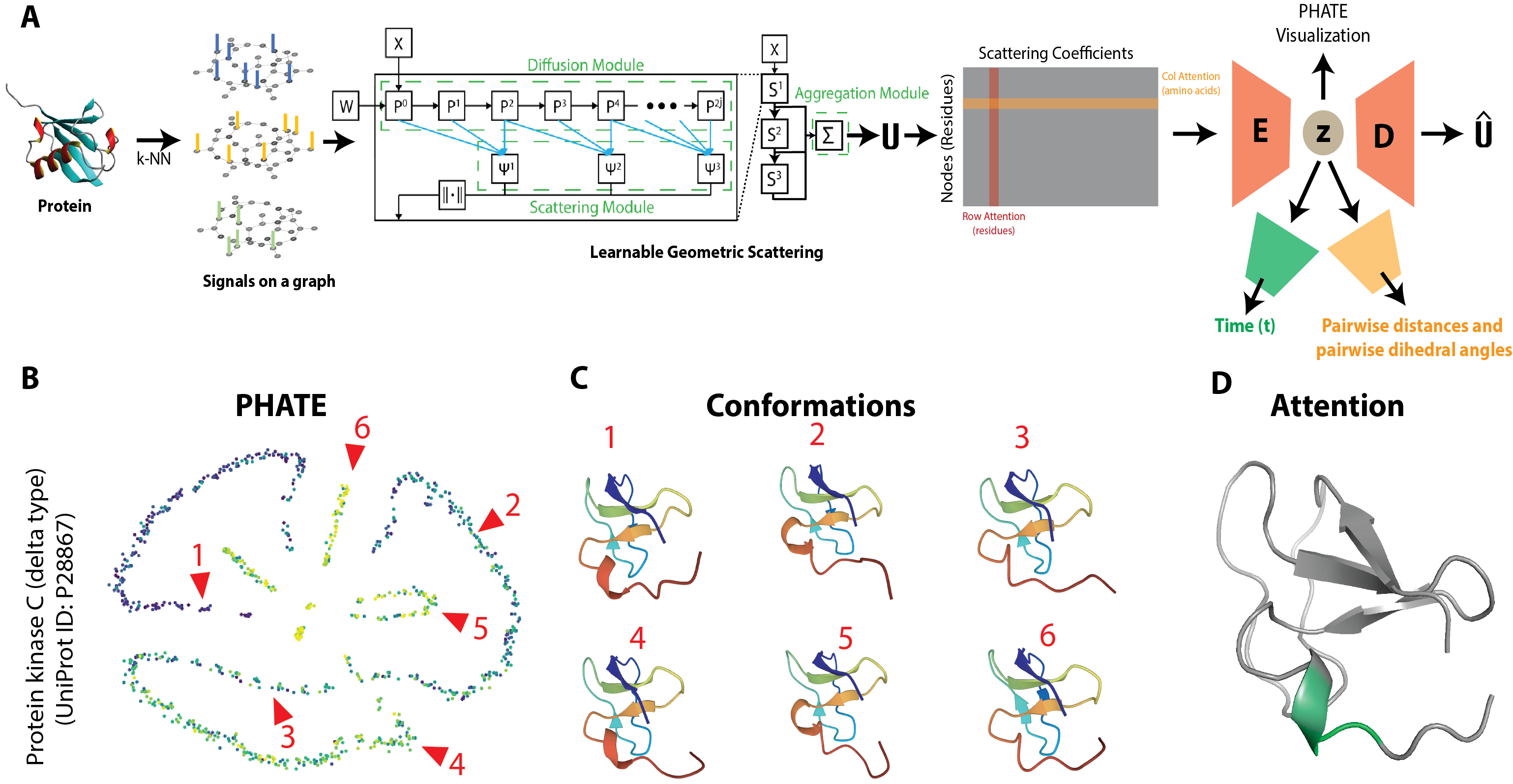
Figure 1: (A) The ProtSCAPE architecture. (B) PHATE plot of latent representations. (C) Conformations of the protein Kinase C. (D) High attention scores correspond to more flexible residues.

2.1 Learnable Geometric Scattering

The geometric scattering transform [10, 11, 12] is a multi-layer, multi-scale, feed-forward feature extractor for processing a signal $\mathbf{x}$ defined on the vertices of a graph $G=(V,E)$. It is built upon diffusion wavelets $\{\Psi_{j}\}_{j=0}^{J}$ defined by $\Psi_{0}=I-P,$ and $\Psi_{j}=P^{2^{j-1}}-P^{2^{j}},1\leq j\leq J,$ where $D$ and $A$ are the degree and adjacency matrices and $P=\frac{1}{2}\left(I+AD^{-1}\right)$ is the lazy random walk matrix. Given these wavelets, first- and second-order scattering coefficients can be defined by $U[j]\mathbf{x}\coloneqq M\Psi_{j}\mathbf{x}$,$U[j_{1},j_{2}]\mathbf{x}\coloneqq M\Psi_{j_{2}}M\Psi_{j_{1}}\mathbf{x}$, where $M\mathbf{x}(v)=|\mathbf{x}(v)|$.

For complex tasks, the pre-chosen dyadic scales, $2^{j}$, used in the definition of $\Psi_{j}$ may be overly rigid. Thus, we instead consider the generalized scattering transform introduced in Tong et al. [9] featuring generalized diffusion wavelets $\widetilde{\mathcal{W}}_{J}=\{\widetilde{\Psi}_{j}\}_{j=0}^{J}$ of the form $\widetilde{\Psi}_{0}=I-P^{t_{1}}$, where $t_{1},\ldots,t_{J+1}$ $\widetilde{\Psi}_{j}\coloneqq P^{t_{j}}-P^{t_{j+1}},\text{ for }1\leq j\leq J,$ is an arbitrary increasing sequence of diffusion scales with $t_{1}\geq 1$ that can be learned in via a differentiable selection matrix. We let $\widetilde{U}[j]\mathbf{x}$ and $\widetilde{U}[j_{1},j_{2}]\mathbf{x}$ denote the generalized scattering coefficients constructed from the $\widetilde{\Psi}_{j}$. We then let $\mathcal{\widetilde{U}}\mathbf{x}$ denote a matrix of all the generalized scattering coefficients associated to $\mathbf{x}$ (where rows correspond to vertices).

2.2 Transformer with Dual Attention

Once the scattering coefficients $\widetilde{\mathcal{U}}\mathbf{x}$ are computed, we use a dual transformer module to obtain multi-headed attention on (1) the residues and (2) the amino acids. We first compute a positional encoding of the scattering coefficients before feeding it into the transformer. For an input of dimensions $n\times d$, the $n\times 2d$ positional encoding matrix $R$ is computed using the cosine encoding method, where $R_{i,2j}=\sin\left(\frac{i}{10000^{2j/d}}\right),R_{i,2j-1}=\cos\left(\frac{i}{10000^{2j/d}}\right)$. We next define $\mathbf{S}=R\|\mathcal{U}\mathbf{x}$, where $\|$ denotes horizontal concatenation. We now feed $\mathbf{S}$ into the Multi-Headed Attention. To do this, we first compute the query $Q$, key $K$, and value $V$ vectors from the input embedding $\mathbf{S}$, $Q=W^{Q}\mathbf{S}$, $K=W^{K}\mathbf{S}$, $V=W^{V}\mathbf{S}$. where $W^{Q},W^{K},$ and $W^{V}$ are learnable weight matrices. We then compute $\operatorname{Attention}(Q,K)=\sigma\left(\frac{QK^{T}}{\sqrt{d_{k}}}\right)$ where $\sigma$ represents the softmax function applied column wise and $d_{k}$ is the number of columns of the query vector $Q$. We then update the values by $V\rightarrow\text{Attention}(Q,K)V.$ We next feed $V$ into a two-layer MLP with ReLU activations.

The second transformer is the same as the first, but applied to $\mathcal{U}^{T}$ (without positional encoding) and computes attention over amino acids rather than the scattering coefficients. The outputs of both transformers are then concatenated to form the final embedding, $\mathbf{p}$.

2.3 Training and Loss Formulation

The embedding $\mathbf{p}$ is fed into an encoder network $E$ in order to compute the latent representation $\mathbf{z}=E(\mathbf{p})$. $\mathbf{z}$ is then passed into three separate modules: two regression networks ($N$ and $M$) and a decoder network $D$. (i) The first regression network $N$ aims to predict the time point $t$ corresponding to each $\mathbf{z}$ and utilizes a mean squared error loss given as $\mathcal{L}_{\text{t}}=\frac{1}{n}\|\hat{t}-t\|^{2}$, $\hat{t}=N(\mathbf{z})$. (ii) The second regression network $M$ aims to predict the pairwise distances and the dihedral angle between residues and also employs a mean squared error loss: $\mathcal{L}_{\text{c}}=\frac{1}{n}\|\hat{C}-C\|^{2}$, where $C$ is the ground truth pairwise distances and dihedral angles and $\hat{C}=M(\mathbf{z})$ is our estimate. (iii) Finally, the scattering coefficients are reconstructed by passing it through a decoder $D$ which consists of a reconstruction loss as $\mathcal{L}_{\text{s}}=\frac{1}{n}\|\hat{\mathcal{U}}\mathbf{x}-\mathcal{U}\mathbf{x}\|^{2}$, where $\hat{\mathcal{U}}\mathbf{x}$$=D(E(\mathbf{p}))$ are the reconstructed scattering coefficients. Our total loss is then given by $\mathcal{L}=\alpha\mathcal{L}_{\text{t}}+\beta\mathcal{L}_{\text{s}}+(1-\alpha+\beta)\mathcal{L}_{\text{c}}.$ However, in the case of large proteins with hundreds of residues, we implement a learnable node embedding strategy to make training more memory-tractable (see Appendix C for details).

Table 1: Mean absolute error (mean $\pm$ std dev. of 20 withheld time windows; lower is better) of decoded mutant structures compared to ground truth at held-out time points. Best results are bold and underlined. Second best results are underlined.

Model	Model	Pairwise Residue COM Distance (MAE $\pm$ std)					Pairwise Residue Dihedral Angle Difference (MAE $\pm$ std)
Family		p.T12P	p.M36G	p.F13E	p.C14I	p.N37P	p.T12P	p.M36G	p.F13E	p.C14I	p.N37P
GNNs	GIN	0.8507 ± 0.0256	0.5191 ± 0.0109	0.5171 ± 0.0095	0.7434 ± 0.0816	4.9396 ± 0.0848	1.3813 ± 0.0244	4.1677 ± 0.0424	1.6896 ± 0.0265	1.4068 ± 0.0217	1.5685 ± 0.0235
	GAT	0.5524 ± 0.0597	0.4869 ± 0.0113	0.4780 ± 0.0116	0.6466 ± 0.0265	0.5760 ± 0.0359	1.7409 ± 0.0355	1.3913 ± 0.0150	1.4044 ± 0.0095	1.5280 ± 0.0321	5.3738 ± 0.0680
	GCN	0.5619 ± 0.0630	37.5953 ± 0.2552	1.0995 ± 0.0161	0.5637 ± 0.0510	0.5471 ± 0.0282	1.8070 ± 0.0293	1.3600 ± 0.0179	1.3731 ± 0.0134	1.4352 ± 0.0260	1.5096 ± 0.0199
	GraphSAGE	0.5456 ± 0.0594	0.4968 ± 0.0056	0.5148 ± 0.0133	0.5756 ± 0.0687	0.6631 ± 0.0233	1.5168 ± 0.0220	1.3662 ± 0.0170	1.4405 ± 0.0112	1.3810 ± 0.0222	1.4005 ± 0.0183
	$E(n)$-EGNN	0.4862 ± 0.0491	0.4660 ± 0.0109	0.4536 ± 0.0070	0.4946 ± 0.0446	0.8045 ± 0.0761	1.3687 ± 0.0199	1.3142 ± 0.0201	1.2891 ± 0.0105	1.3854 ± 0.0265	1.4127 ± 0.0285
Ours	w/o time regression	0.2559 $\pm$ 0.0889	0.1439 $\pm$ 0.0143	0.1350 $\pm$ 0.0148	0.2642 $\pm$ 0.1041	0.3058 $\pm$ 0.0492	0.9117 $\pm$ 0.1276	0.7722 $\pm$ 0.0696	0.6980 $\pm$ 0.0581	1.0470 $\pm$ 0.2309	1.0323 $\pm$ 0.1007
	w/o attention	0.8581 $\pm$ 0.0404	0.5075 $\pm$ 0.0352	0.2054 $\pm$ 0.0159	0.4502 $\pm$ 0.0971	0.6302 $\pm$ 0.0544	1.3848 $\pm$ 0.1259	0.8957 $\pm$ 0.0386	0.7158 $\pm$ 0.0509	1.0400 $\pm$ 0.1831	1.0479 $\pm$ 0.0680
	ProtSCAPE	0.2506 ± 0.0947	0.1261 ± 0.0132	0.1173 ± 0.0124	0.2651 ± 0.1083	0.3070 ± 0.0504	0.9028 ± 0.1249	0.7614 ± 0.0670	0.6873 ± 0.0565	1.0351 ± 0.2268	1.0225 ± 0.1004

3 Experimental Results

We consider MD simulations of proteins, which provide 3-D coordinates of the protein at an atomic resolution at multiple time points (frames). We coarse-grain the atomic coordinates to compute the center of mass of each residue in the protein and construct an unweighted $k$-NN graph ($k=5$) of the protein structure with residues as vertices and undirected edges between all residues within $k$-neighborhood distance. We train ProtSCAPE on datasets consisting of graphs of the same protein at different time points in the MD simulation. The model is trained to learn latent representations of the protein, from which we predict the pairwise distances of the center of mass of the residues as well as the pairwise dihedral angles of the residues in the protein. Note that the number of residues remains constant during the simulation. We uniformly sample and withhold 20 windows of 10 time points each, train our model on the remaining time points and evaluate our model based on its ability to reconstruct the pairwise distances and dihedral angles of the withheld points. Interpolation results on three different proteins in the ATLAS database [13] are provided in Appendices D and E. We evaluate the organization of the latent representations in Appendix F. In Appendix G, we analyze MD simulations of the GB3 protein, showing that ProtSCAPE can identify stochastic switching between two meta-stable conformations.

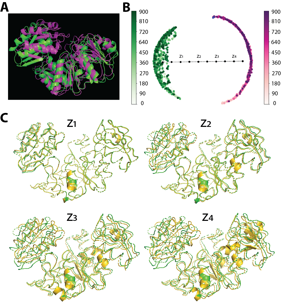
Figure 2: Interpolation between open and closed conformations of the MurD protein

Latent interpolation of open-close transition in MurD

The MurD (UDP-N-acetylmuramoyl-L-alanine:D-glutamate ligase) [14] protein exists in open and closed conformation as seen in Figure 2(A). In the open conformation the ligands are able to bind to the pockets in the protein whereas in closed conformation, the pockets are blocked hence preventing ligand binding. We use the MD simulations of the open and closed states [15] to train ProtSCAPE and obtain the latent representations of the MurD protein. As seen in Figure 2(B), the PHATE visualization of latent representations shows two clusters corresponding to the open and closed conformations (colored by green and purple respectively) in the latent representations. We construct a linear interpolant between the cluster centroids of the open and closed states and decode their intermediate structures. We visualize these intermediate structures transitioning from open to close states using PyMoL, revealing a hinge-like mechanism. Note that the structures of the open and closed states [16, 17] as well as the intermediate states [18] of MurD have been experimentally determined, and the hinge mechanism obtained by ProtSCAPE is consistent with the experimental findings.

Generalizability

We demonstrate that ProtSCAPE generalizes from short-to-long (S2L) trajectories and from wildtype-to-mutant (WL2M) trajectories. In Appendix H, we show that the model trained on short trajectories can successfully embed and reconstruct long trajectories. In Appendix I, we show that the model trained on wildtype trajectories can effectively embed and reconstruct dynamics of missense mutations (single substitution mutants). Table 1 shows that ProtSCAPE is the best performing model when compared to GNNs in terms of decoding mutant structures.

Appendix

A Related Works

Computational biology has witnessed substantial interest in understanding protein dynamics, protein-protein interactions, protein-ligand interactions, and protein-nucleic acid interactions. Numerous computational methods have been developed to address determination of protein tertiary structure from the primary amino acid sequence (protein folding), predicting mutational stability, and determining binding sites and binding affinity in biomolecular interactions. However, the exploration of protein dynamics in molecular dynamics (MD) simulations using machine learning techniques has not been as extensively pursued.

A.1 Advances in Static Protein Structure Prediction

A significant breakthrough in the field of static protein structure prediction has been achieved with the development of DeepMind’s AlphaFold model and related models [19, 20, 21, 22]. These tools have shown exceptional effectiveness in determining the three-dimensional configurations of proteins based solely on their amino acid sequences. However, these tools primarily produce models of proteins in their equilibrium state, providing snapshots of their structures under static conditions rather than capturing dynamic fluctuations and conformational changes. Nevertheless, understanding these dynamic aspects is crucial for comprehending how proteins function in more complex biological systems and how they respond to different environmental stimuli.

A.2 Traditional Analytical Techniques in Protein Dynamics

Traditionally, the study of dynamic changes in protein structures has heavily relied on the analysis of molecular dynamics (MD) trajectories. Key analytical methods include examining dihedral and torsion angles, which are critical for understanding the rotation around bonds within the protein backbone and side chains. Many analyses rely on root mean square fluctuations (RMSF), which measures the deviation of parts of the protein structure from their average positions over time, providing insights into the flexibility and dynamic regions of the protein. Ramachandran plots [23] are also widely used, offering a visual and quantitative assessment of the sterically allowed and forbidden conformations of dihedral angles in protein structures. These plots encode the conformational landscape of proteins, by showing the frequency of occurrence of dihedral angle pairs in various conformations. These techniques primarily focus on local conformational changes and often do not adequately capture the global interactions within and between different motifs and domains of the protein. Additionally, they fail to capture transient interactions and rapid conformational shifts that are essential for understanding the protein’s full biological functionality.

A.3 Traditional Analytical Techniques in Protein Dynamics

Recent efforts in machine learning have shifted towards leveraging such features extracted from MD trajectories to enhance our understanding of protein dynamics. The MDTraj (McGibbon et al. [24]) suite, for instance, offers a comprehensive toolkit for analyzing these trajectories through various computed features, such as radius of gyration, solvent-accessible surface area, torsion angles, etc. In the realm of deep learning, methods such as dynamic tensor analysis (Sun et al. [25]) have been explored to discern patterns in protein dynamics more effectively. Ramanathan et al. [26] have pioneered work in this area by representing protein trajectories as tensors to identify conformational substates and differentiate between stable and dynamic phases within MD simulations.

In this work, we take a representation learning approach to understanding the dynamics of conformational changes in proteins, by learning a latent representation that can be decoded back to the protein structure, and is temporally organized to enable interpolation between protein conformations. Our approach most closely resembles that of Ramaswamy et al. [27], who implement a CNN autoencoder, with a physics-informed loss function to ensure physically-plausible intermediate transition paths between equilibrium states. However, their model requires a relatively computationally-expensive feature set of physics-based electrostatics and potentials, and they also found that in inference, it may yet miss finer domain-level conformational changes and produce suboptimal loop regions where the protein is more flexible (Ramaswamy et al. [27], p. 8).

B Theoretical Results

In this section, we will state two theorems which, when taken together, show that the generalized geometric scattering transform, a key ingredient in our architecture, is stable to small perturbations, i.e., it will represent molecules in similar ways if the molecules have the similar structure. For proofs, please see Appendix J.

In addition to the theorems stated below, we also note that Theorem 2 of [9] shows that the generalized graph scattering coefficients $\widetilde{\mathcal{U}}$ are permutation equivariant, i.e., if you reorder the vertices, you reorder each scattering coefficient in the same manner. Therefore, this result, together with our theorems below shows that the generalized geometric scattering transform captures the intrinsic structure of the data rather than superficial artifacts such as the ordering of the vertices and is stable to small perturbations of the graph.

Let $G^{\prime}=(V^{\prime},E^{\prime})$ denote a graph which is interpreted as a perturbed version of $G=(V,E)$ and satisfies the same assumptions as $G,$ e.g., that is connected. For any object $X$ associated to $G$, we will let $X^{\prime}$ represent the analogous object on $G^{\prime}$, for instance, $A^{\prime}$ and $D^{\prime}$ will denote the adjacency and degree matrices of $G^{\prime}$. In order to quantify the differences between $G$ and $G^{\prime}$ we will introduce several quantities. First, we define

$$\kappa\coloneqq\max\{\|I-D^{-1/2}(D^{\prime})^{1/2}\|_{2},\|I-(D^{\prime})^{-1/2}D^{1/2}\|_{2}\},$$ (1)

where here and throughout $\|M\|$ denotes the $\ell^{2}$ operator norm of a matrix $M$, i.e., $\|M\|=\sup_{\|\mathbf{x}\|_{2}=1}\|M\mathbf{x}\|_{2}$. Notably, if $D=D^{\prime}$, e.g., if both $G$ and $G^{\prime}$ are $k$-regular graphs, we will have $\kappa=0$. More generally, $\kappa$ will be small if $G$ and $G^{\prime}$ have similar degree vectors. Next, we let

$$R\coloneqq\max\{\|D^{-1/2}(D^{\prime})^{1/2}\|,\|(D^{\prime})^{-1/2}D^{1/2}\|\},$$ (2)

and observe that if $G$ and $G^{\prime}$ have similar degree vectors we have $R\approx 1$. Lastly, following the lead of Perlmutter et al. [28] and Gama et al. [11] we consider the diffusion distance $\|P-P^{\prime}\|_{D^{-1/2}},$ where $\|M\|_{D^{-1/2}}=\sup_{\|\mathbf{x}\|_{D^{-1/2}}=1}\|M\mathbf{x}\|_{D^{-1/2}}$ denotes the operator norm of a matrix $M$ on the weighted $\ell^{2}$ space $\|\mathbf{x}\|_{D^{-1/2}}=\|D^{-1/2}\mathbf{x}\|_{2}=\sum_{v\in V}\frac{|\mathbf{x}(v)|^{2}}{\mathbf{d}(v)}.$ Our first theorem, provides stability of the generalized wavelets $\tilde{\mathcal{W}}_{J}$ by bounding

$$\|\tilde{\mathcal{W}}_{J}-\tilde{\mathcal{W}}^{\prime}_{J}\|_{D^{-1/2}}\coloneqq\left(\sum_{j=0}^{J}\|\widetilde{\Psi_{j}}\mathbf{x}-\widetilde{\Psi_{j}}^{\prime}\mathbf{x}\|_{D^{-1/2}}^{2}\right)^{1/2}.$$

It builds off of the results obtained in Theorems 4.2 and 4.3 in Perlmutter et al. [28] which considered the dyadic wavelets $\Psi_{j}$ (see also Proposition 4.1 of Gama et al. [11]). The constant in our bound will depend on the spectra of $P$ and $P^{\prime}$. It is known that the largest eigenvalue of $P$ is given by $\lambda_{1}=1$ and since $G$ is connected, the second largest eigenvalue satisfies $1=\lambda_{1}>\lambda_{2}>0$. This second eigenvalue can be interpreted as measuring how strongly connected the graph is. If the spectral gap $1-\lambda_{2}$ is small, then the graph is thought of as being nearly disconnected, whereas if the spectral graph is large, the graph is thought of as being more tightly connected.

Theorem B.1.

The wavelet transform is stable to small graph perturbations. More specifically, let $G^{\prime}=(V^{\prime},E^{\prime})$ be a perturbed version of $G$ with $|V|=|V^{\prime}|=n$. Then

$$\|\tilde{\mathcal{W}}_{J}-\tilde{\mathcal{W}}^{\prime}_{J}\|_{D^{-1/2}}^{2}\leq C\left(\kappa(1+R^{3})+R\|P-P^{\prime}\|_{D^{-1/2}}+\kappa^{2}(\kappa+1)^{2}\right),$$

where $C$ is a constant depending only on the spectral gaps of the graphs $G$ and $G^{\prime}$ and in particular does not depend on $J$ or on the choice of scales $t_{j}$.

To understand this result, we note that if $G$ is close to $G^{\prime}$ in the sense that $A^{\prime}\approx A$, we will have $\kappa\approx 0$ and $R\approx 1.$ Therefore, we will have $\|\tilde{\mathcal{W}}_{J}-\tilde{\mathcal{W}}^{\prime}_{J}\|_{D^{-1/2}}^{2}\lesssim C\|P-P^{\prime}\|_{D^{-1/2}}$.

Our next theorem builds on Theorem B.1 to show that the $\ell$-th order scattering coefficients are also stable to the minor perturbation of the graph structure. Notably, our stability bound in Theorem B.1, and therefore B.2, does not depend n the number of wavelet scales used, $J$, or the choice of scales $t_{j}$. This fact, which is in part a consequence of the wavelets being designed to capture complementary information stands in contrast to analogous results for generic (non-wavelet based) GNNs (see, e.g., Theorem 4 of [29]) where the stability bounds rapidly increase with the size of the filter bank.

Theorem B.2.

The generalized geometric scattering $\tilde{U}$ transform is stable to small deformations of the graph structure. In particular, for all $\mathbf{x}\in\mathbb{R}^{n}$, and $R$ as in (2), we have

$$\sum_{0\leq j_{1},\ldots,j_{\ell}\leq J}\|\widetilde{U}[j_{1},\ldots,j_{\ell}]\mathbf{x}-\widetilde{U}^{\prime}[j_{1},\ldots,j_{\ell}]\mathbf{x}\|^{2}_{D^{-1/2}}\leq\|\tilde{\mathcal{W}}_{J}-\tilde{\mathcal{W}}^{\prime}_{J}\|_{D^{-1/2}}^{2}\left(\sum_{k=0}^{\ell-1}R^{2k}\right)^{2}\|\mathbf{x}\|^{2}_{D^{-1/2}}.$$

C Learnable Node Embeddings

In most of our experiments, we will generally take our input signals $\mathbf{x}$ to be one-hot encodings of the amino acids. However, in cases where the protein has a large number of residues which corresponds to large graph size, the use of a one-hot encoding of the amino acids as node features results in a significant increase in model parameters. This leads to vast memory requirements for model execution. Hence, we consider the use of an autoencoder to generate learnable 3-D node embeddings in order to optimize for memory. The encoder and decoders are both defined to be multilayer perceptrons that consist of 2 linear layers with a ReLU activation in between them. The encoder takes as input the signals $\mathbf{x}$ constructed through a one-hot encoding of the amino acids and produces a 3-D embedding of the residues. This 3-D embedding is then utilized as node features of the graphs for the model. The decoder then reconstructs the one-hot encoding of the amino acids back from the 3-D embedding. In these cases, we also utilize a reconstruction loss $\mathcal{L}_{n}=\frac{1}{n}\|\hat{\mathbf{x}}-\mathbf{x}\|^{2}$ where $\hat{\mathbf{x}}$ is the reconstructed one-hot encoding of the amino acids. Our total loss $\mathcal{L}$ is then defined by

$$\mathcal{L}=\alpha\mathcal{L}_{\text{t}}+\beta\mathcal{L}_{\text{s}}+\gamma\mathcal{L}_{\text{c}}+(1-\alpha-\beta-\gamma)\mathcal{L}_{n}$$

where $\alpha$, $\beta$, and $\gamma$ are tunable hyperparameters.

D Interpolation of pairwise distances at withheld time points

We obtained short MD simulations of three proteins (Hirustasin, 50S Ribosomal Protein L30, Protein Kinase C Delta) from the ATLAS open online repository [13] consisting of 1000 frames sampled at a rate of approximately one frame per 100 picoseconds.

We visualize the latent representations obtained from the encoder using the PHATE [30] dimensionality reduction algorithm. As shown in Figure 3, the latent representations are organized by time, with different regions of the latent space corresponding to distinct protein conformations. Furthermore, in Figure 3, we visualize the attention scores learned by the transformer using PyMOL [31]. Residues with high attention scores, colored in green, indicate more significant contributions to the latent representation obtained by ProtSCAPE. We note that these residues correspond to more flexible regions of the protein that play a pivotal role in conformational changes.

Additionally, as shown in Table 2, ProtSCAPE outperforms other graph-based methods (GNNs) in predicting pairwise distances between the center of mass of the residues as well as pairwise residue dihedral angle differences indicating that ProtSCAPE excels in capturing the spatial and angular relationships in protein conformations. We note that the full version of ProtSCAPE does perform slightly worse than the versions without the attention or without the time-regression. However, these differences are small and the addition of the time-regression leads to a more coherently structured latent space while the attention mechanism makes the model more interpretable.

Table 2: MAE (mean $\pm$ std dev.) of decoded structures compared to ground truth at held-out timepoints. (Lower is better.) Best results are bold and underlined. Second best results are underlined.

Model	Model	Pairwise Residue COM Distance			Pairwise Residue Dihedral Angle Difference
Family		1ptq	1bxy	1bx7	1ptq	1bxy	1bx7
GNNs	GIN	0.6017 ± 0.0071	0.6300 ± 0.0014	0.8094 ± 0.0210	87.7973 ± 0.0220	1.3894 ± 0.0027	1.4380 ± 0.0086
	GAT	0.6033 ± 0.0076	0.4984 ± 0.0022	0.6856 ± 0.0189	1.3894 ± 0.0080	26.7543 ± 0.0143	1.4467 ± 0.0183
	GCN	4.0285 ± 0.0160	5.9410 ± 0.0133	1.4184 ± 0.0067	1.4184 ± 0.0067	1.6042 ± 0.0043	3.1116 ± 0.0445
	GraphSAGE	0.4686 ± 0.0055	0.4956 ± 0.0019	0.6828 ± 0.0196	1.3906 ± 0.0082	1.8634 ± 0.0100	1.4318 ± 0.0156
	$E(n)$-EGNN	0.5345 ± 0.0018	0.5239 ± 0.0014	0.8144 ± 0.0330	1.3955 ± 0.0090	1.3837 ± 0.0024	1.4679 ± 0.0099
Ours	w/o time regression	0.0715 ± 0.0120	0.0545 ± 0.0079	0.1134 ± 0.0289	0.4425 ± 0.0423	0.2683 ± 0.0247	0.6061 ± 0.0731
	w/o attention	0.0711 ± 0.0098	0.0531 ± 0.0068	0.1058 ± 0.0230	0.4440 ± 0.0450	0.2724 ± 0.0356	0.6050 ± 0.0675
	ProtSCAPE	0.0735 ± 0.0125	0.1248 ± 0.0251	0.1184 ± 0.0285	0.4548 ± 0.0481	0.3055 ± 0.0424	0.6155 ± 0.0644

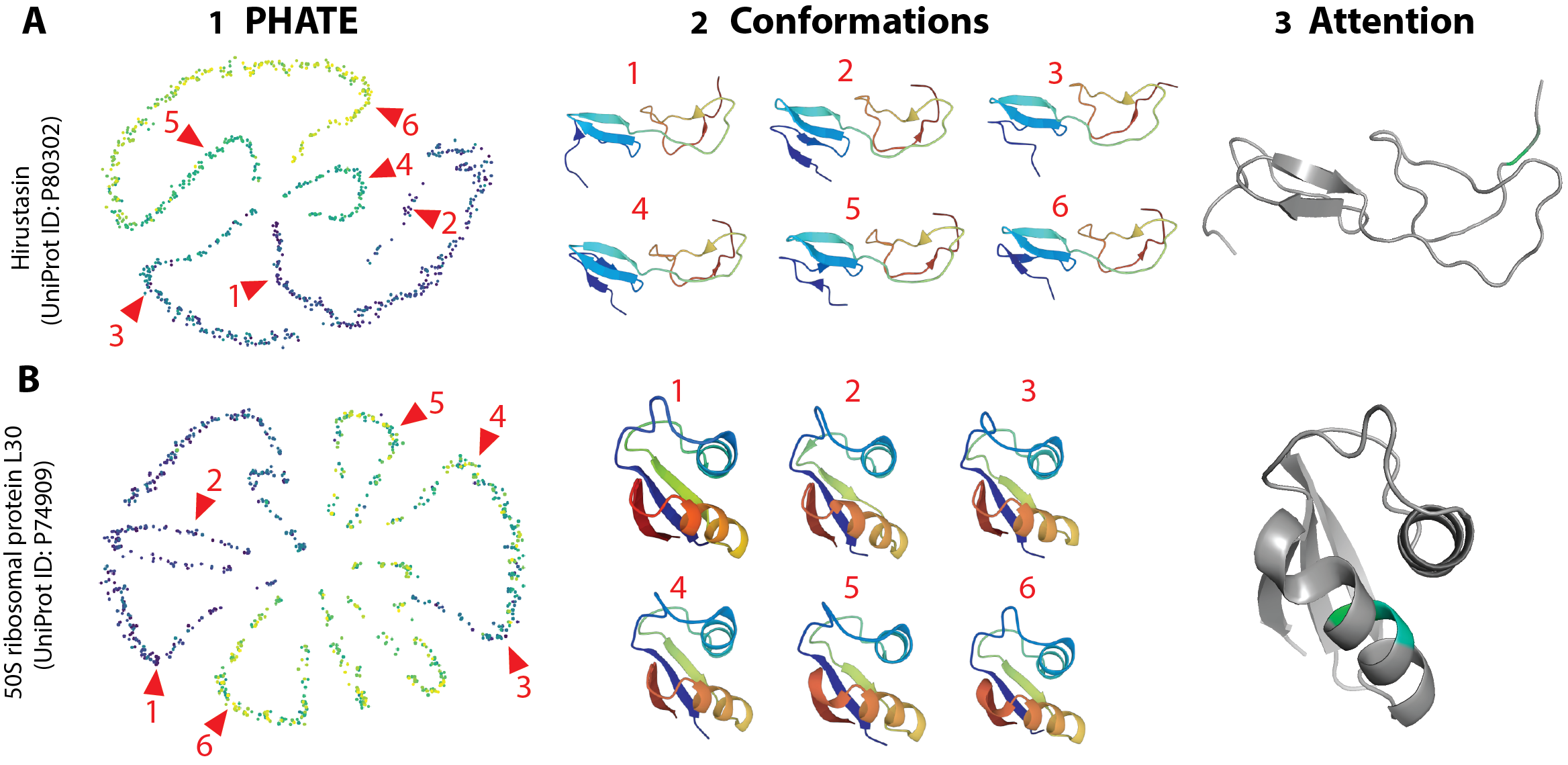
Figure 3: Representation of the latent space (1), conformation samples(2) and Attention read-outs(3) for two different proteins simulations: Hirustasin(A) and 50S Ribosomal protein L30 (B). As we can see the attention is higher on parts of the protein that are flexible (i.e. change over different time points)

E Interpolation of residue coordinates at withheld time points

In additional to training the equivariant ProtSCAPE architecture that reconstructs pairwise distances and angles between residues, we also trained a variant of the model that directly reconstructs residue center of mass coordinates from the latent representation. In this section, we report the performance of this model using four metrics, Spearman Correlation Coefficient (SCC; higher is better), Pearson Correlation Coefficient (PCC; higher is better), Root Mean Square Distance (RMSD; lower is better), and Discrete Optimized Protein Energy (DOPE; lower is better). To evaluate using SCC and PCC, we compared the ground truth pairwise Euclidean distances between residue centers with the distances between the reconstructed residue coordinates at withheld time points. RMSD and DOPE were calculated from atomic coordinates by placing amino acids at the reconstructed residue coordinates obtained from ProtSCAPE and comparing against the withheld ground truth structure. DOPE scores were calculated using the MODELLER package.

We compared the performance of ProtSCAPE against GNNs and deep learning models trained using features derived from MDTraj [24] and Ramachandran plots using these metrics. As shown in Table 3, ProtSCAPE is overall the top performing model with best, or second best, performance across all five proteins of interest. MD trajectories of these proteins were obtained from the ATLAS [13] and D. E. Shaw Research datasets (GB3 and BPTI). A recurrent neural network trained on MDTraj-derived features, denoted MDTraj-RNN, is overall the second best performing method with regards to SCC and PCC. A variational autoencoder trained on MDTraj-derived features, denoted MDTraj-VAE, is overall the second best performing method with respect to RMSD. However, it is the worst performing method with respect to SCC and PCC. In comparison, the convolutional model trained on Ramachandran features generally does not perform well on any of the methods or datasets.

To visualize the reconstructed protein structure at withheld timepoints, we obtained atomic coordinates by placing amino acids at the predicted center of mass of the residues. This generated an imperfect atomic-scale reconstruction, since the precise orientation of the residues is not predicted. Consequently, when the reconstructed protein is visualized using PyMOL (Figure 4), the alpha folds and beta sheets are not rendered, even through the location of the residues matches the ground-truth. This artifact can be fixed in the future versions by predicting the orientation of the residue in additional to its center of mass through the decoder.

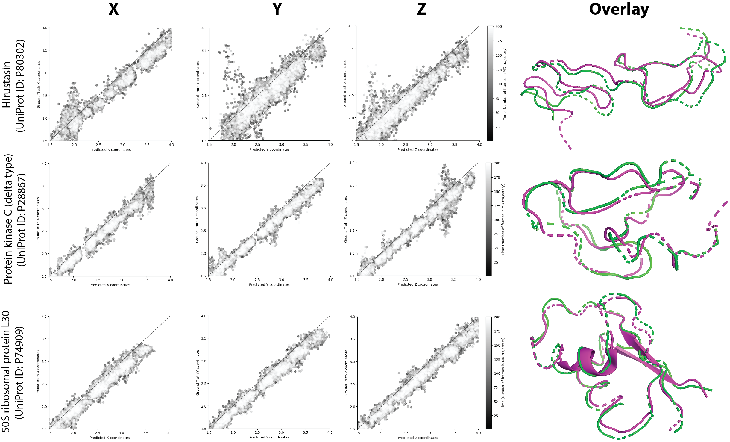
Figure 4: Plots of ground truth vs. reconstructed residue coordinates at withheld time points. The overlay shows good agreement between the ground truth structure (colored in magenta) and the ProtSCAPE reconstructed structure (colored in green) obtained by decoding the latent representations of the protein structure at withheld timepoints.

Table 3: Reconstruction metrics (mean $\pm$ std dev. computed using five-fold cross-validation).
Best results are bold and underlined. Second best results are underlined.

Model	Protein	SCC ($\uparrow$)	PCC ($\uparrow$)	RMSD ($\downarrow$)	DOPE ($\downarrow$)
MDTraj-VAE	Hirustasin	$0.28\pm 0.08$	$0.28\pm 0.08$	$0.40\pm 0.01$	$\;\,\underline{\mathbf{862.5\pm 1.32}}$
	50S Ribosomal	$0.42\pm 0.09$	$0.44\pm 0.05$	$\underline{0.15\pm 0.00}$	$\underline{1243.4\pm 0.24}$
	Protein Kinase C	$0.41\pm 0.07$	$0.36\pm 0.01$	$\underline{0.25\pm 0.00}$	$\;\,\underline{\mathbf{1078.8\pm 0.16}}$
	GB3	$0.30\pm 0.15$	$0.22\pm 0.16$	$\underline{\mathbf{0.38\pm 0.00}}$	$\underline{1117.3\pm 0.09}$
	BPTI	$0.35\pm 0.06$	$0.24\pm 0.11$	$\underline{\mathbf{0.36\pm 0.00}}$	$\;\,\underline{\mathbf{1155.2\pm 0.10}}$
MDTraj-RNN	Hirustasin	$\underline{0.76\pm 0.02}$	$\underline{0.74\pm 0.01}$	$\underline{0.38\pm 0.01}$	$982.73\pm 2.06$
	50S Ribosomal	$\underline{0.79\pm 0.01}$	$\underline{0.76\pm 0.01}$	$0.23\pm 0.00$	$\;\,\underline{\mathbf{1186.32\pm 1.73}}$
	Protein Kinase C	$\underline{0.72\pm 0.02}$	$\underline{0.68\pm 0.01}$	$0.29\pm 0.00$	$1104.47\pm 1.17$
	GB3	$\underline{\mathbf{0.63\pm 0.01}}$	$\underline{\mathbf{0.61\pm 0.03}}$	$1.24\pm 0.13$	$\;\,\underline{\mathbf{1068.53\pm 2.37}}$
	BPTI	$\underline{\mathbf{0.68\pm 0.02}}$	$\underline{0.66\pm 0.01}$	$1.59\pm 0.26$	$\underline{1256.03\pm 1.79}$
Ramachandran ConvNet	Hirustasin	$0.37\pm 0.06$	$0.32\pm 0.05$	$0.61\pm 0.04$	$1414.62\pm 2.10$
	50S Ribosomal	$0.42\pm 0.04$	$0.38\pm 0.04$	$0.57\pm 0.01$	$1285.29\pm 3.64$
	Protein Kinase C	$0.29\pm 0.11$	$0.24\pm 0.03$	$0.83\pm 0.04$	$1298.62\pm 1.30$
	GB3	$0.37\pm 0.08$	$0.37\pm 0.10$	$1.64\pm 0.19$	$1237.09\pm 2.26$
	BPTI	$0.26\pm 0.06$	$0.24\pm 0.03$	$1.92\pm 0.23$	$1329.44\pm 1.97$
GCN	Hirustasin	$0.93\pm 0.01$	$0.93\pm 0.01$	$0.42\pm 0.01$	$925.66\pm 4.27$
	50S Ribosomal	$0.93\pm 0.00$	$0.93\pm 0.00$	$0.32\pm 0.01$	$1284.30\pm 2.95$
	Protein Kinase C	$0.94\pm 0.00$	$0.93\pm 0.00$	$0.34\pm 0.01$	$1101.51\pm 2.32$
	GB3	$0.44\pm 0.03$	$0.42\pm 0.03$	$0.90\pm 0.02$	$1195.75\pm 8.74$
	BPTI	$0.58\pm 0.04$	$0.57\pm 0.04$	$0.94\pm 0.03$	$\underline{1257.90\pm 3.96}$
GIN	Hirustasin	$0.96\pm 0.00$	$0.96\pm 0.00$	$0.37\pm 0.02$	$919.12\pm 5.45$
	50S Ribosomal	$0.97\pm 0.00$	$0.96\pm 0.00$	$0.26\pm 0.02$	$1285.05\pm 1.50$
	Protein Kinase C	$0.96\pm 0.00$	$0.96\pm 0.00$	$0.30\pm 0.01$	$1101.81\pm 2.64$
	GB3	$0.37\pm 0.05$	$0.36\pm 0.04$	$0.95\pm 0.02$	$1201.17\pm 9.40$
	BPTI	$0.47\pm 0.08$	$0.46\pm 0.08$	$0.98\pm 0.03$	$1270.83\pm 5.50$
GAT	Hirustasin	$0.96\pm 0.00$	$0.96\pm 0.00$	$0.36\pm 0.01$	$1097.23\pm 1.25$
	50S Ribosomal	$0.96\pm 0.00$	$0.96\pm 0.00$	$0.27\pm 0.00$	$1272.84\pm 1.49$
	Protein Kinase C	$0.96\pm 0.00$	$0.95\pm 0.00$	$0.30\pm 0.01$	$1097.23\pm 1.25$
	GB3	$0.43\pm 0.03$	$0.42\pm 0.04$	$0.92\pm 0.02$	$1194.86\pm 6.89$
	BPTI	$0.61\pm 0.03$	$0.60\pm 0.02$	$0.95\pm 0.02$	$\underline{1257.01\pm 9.69}$
ProtSCAPE	Hirustasin	$\underline{\mathbf{0.97\pm 0.00}}$	$\underline{\mathbf{0.97\pm 0.00}}$	$\underline{\mathbf{0.24\pm 0.00}}$	$\underline{872.97\pm 0.63}$
	50S Ribosomal	$\underline{\mathbf{0.96\pm 0.05}}$	$\underline{\mathbf{0.95\pm 0.06}}$	$\underline{\mathbf{0.12\pm 0.00}}$	$\underline{1244.26\pm 2.40}$
	Protein Kinase C	$\underline{\mathbf{0.98\pm 0.00}}$	$\underline{\mathbf{0.98\pm 0.00}}$	$\underline{\mathbf{0.20\pm 0.04}}$	$\underline{1080.16\pm 0.83}$
	GB3	$\underline{0.60\pm 0.02}$	$\underline{0.60\pm 0.01}$	$\underline{0.86\pm 0.07}$	$1196.03\pm 23.54$
	BPTI	$\underline{0.66\pm 0.07}$	$\underline{\mathbf{0.67\pm 0.06}}$	$\underline{0.96\pm 0.02}$	$1264.99\pm 11.31$

F Smoothness of latent representation

In order to quantitatively measure the smoothness of the temporally organized latent representations, we constructed a $k$-NN graph from the latent representations and then computed the Dirichlet energy as follows:

$$\mathcal{E}(\mathbf{x})=\frac{\mathbf{x}^{T}L\mathbf{x}}{\mathbf{x}^{T}\mathbf{x}},$$ (3)

where $L$ is the Laplacian of the $k$-NN graph and $\mathbf{x}$ is a vector containing the time (frame number) corresponding to each protein in the same order in which it appears in $L$.

Table 4: Dirichlet energy (lower is better).

Model	Hirustasin	50S Ribosomal	Protein Kinase C	GB3	BPTI
MDTraj-VAE	$0.704$	$0.683$	$0.616$	$0.371$	0.326
Ramachandran ConvNet	$\underline{0.376}$	$\underline{0.401}$	$\underline{0.452}$	$\underline{0.583}$	$\underline{0.661}$
ProtSCAPE	$\mathbf{1.959\times 10^{-9}}$	$\mathbf{2.084\times 10^{-9}}$	$\mathbf{1.722\times 10^{-16}}$	$\mathbf{7.080\times 10^{-4}}$	$2.101$

Table 4 compares the Dirichlet energy of latent representations obtained using various baselines from MD trajectories of proteins in the ATLAS and D. E. Shaw Research datasets. We see that the latent representations obtained from ProtSCAPE have the lowest Dirichlet energy compared to the baselines, demonstrating its ability to capture smooth and temporally organized latent representations.

G ProtSCAPE uncovers stochastic switching between conformations in the GB3 protetin

In this case study, we considered a $10\mu$s MD trajectory of the GB3 protein provided by D. E. Shaw Research. We obtained latent representations of the GB3 trajectory using ProtSCAPE and observed that it exhibits stochastic switching between two conformations, with stochastic back-and-forth transitions over time (see Figure 5B). Specifically, we noticed the presence of two clusters in the latent embeddings, with each cluster organized temporally, and each cluster corresponding to different conformation of the protein. By segmenting the two clusters, we showed that the protein transitions between an open loop and a closed loop conformation.

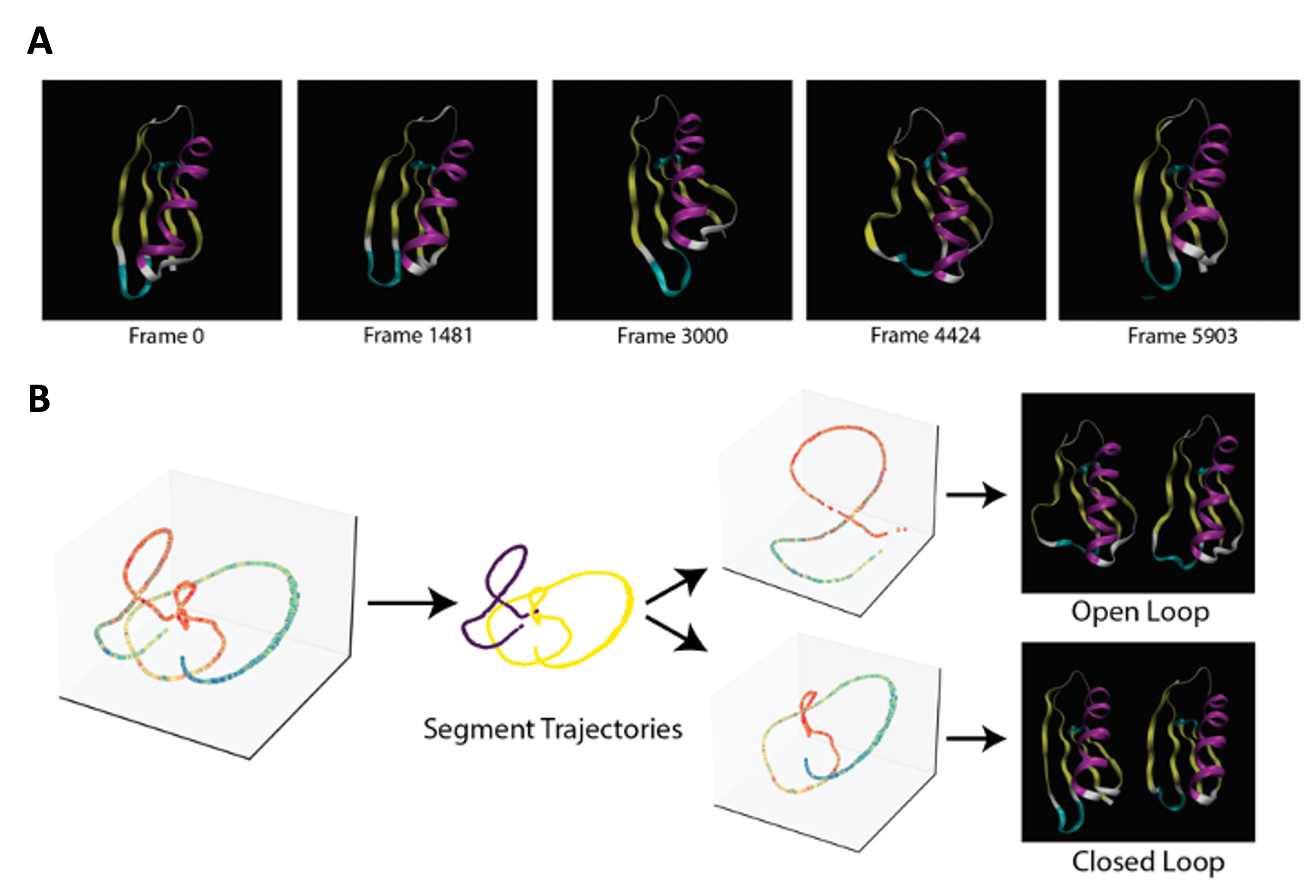
Figure 5: (A) describes the GB3 protein changing conformations at different timepoints in the molecular dynamics simulation. (B) Latent representations captured by ProtSCAPE visualized using PHATE

H ProtSCAPE generalizes from short to long trajectories

We trained ProtSCAPE on short trajectories containing 1000 frames and evaluated it on long trajectories containing 10,000 frames in the ATLAS [13] dataset. The model trained on short trajectories was used to embed and decode frames in the longer trajectory (see Figure 6). We observed that despite being trained only on short trajectories, ProtSCAPE can still create an organized latent space for longer trajectories, showing that the model is not limited by it’s time component and can infer an organized latent space even for unseen poses and dynamics. This demonstrates that ProtSCAPE inherently learned to represent protein structure based on dynamics, not only the specific timescale and conformations it was trained on, but in general for a given protein. In future work, we will test the limitations of ProtSCAPE in extrapolating from short to long trajectories.

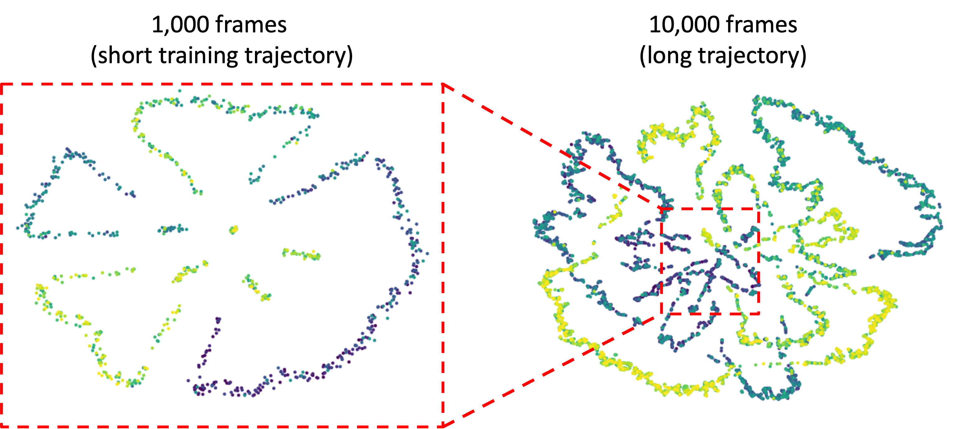
Figure 6: PHATE plots of latent representations obtained using short and long MD trajectories of Protein Kinase C. ProtSCAPE was trained on short (1,000 frames) trajectories and evaluated on long (10,000 frames) trajectories.

I ProtSCAPE generalizes from wild-type to mutant trajectories

To assess the generalization capability of ProtSCAPE for mutant proteins, we first had to obtain mutant protein structures and perform MD simulations. Due to the combinatorial complexity of generating structures of all possible mutations, we restricted our analysis to a limited set of missense mutations, obtained by substituting one residue in the protein sequence. To generate these mutants, we retrieved the attention scores over the residues and chose the residues with the highest attention scores as the target for mutation. For example, residue 37 had the highest attention score in Protein Kinase C, so we chose to generate mutants by substituting the amino acid at this residue. To choose to which amino acid to substitute, we used the Sneath’s index [32] - obtaining the most dissimilar amino acids to generate a missense mutation. In our Protein Kinase C example, residue 37 is Asparagine (N), so we substituted it for Proline (P), which is the most dissimilar amino acid to Asparagine according to the Sneath’s index.

To generate mutant MD simulations, we started with the wild-type (WT) folded structure available at ATLAS [13] and used the PyMOL Mutagenesis tool [31] to generate the specific mutation in the protein structure (e.g. N to P). Using the mutated protein structure, we performed MD simulations using the same procedure described in the ATLAS dataset [13]. We used GROMACS [33] to place the protein in a triclinicbox, solvated it using TIP3P water molecules and neutralized with ${Na}^{+}/{Cl}^{-}$ ions. We then perform a step of energy minimization, followed by an equilibration in an NVT ensemble and an NPT ensemble. Finally, we ran the production molecular dynamics simulation using random starting velocities. To obtain the final simulation trajectory, we centered the protein and removed any ions and solvates from the structure, retrieving the 100ns of the simulation trajectory.

We show the latent representations of the mutant and WT protein in Figure 7. We label the mutants using the following notation: p.WxxM where W is the wild-type amino acid, xx is the residue position and M is the mutated amino acid (e.g. pN37P).

From Figure 7A we observe that the MD trajectories of the mutants resemble those of the WT proteins, with significant overlap in the latent representations. However, in some substitutions with high levels of dissimilarity, we observe that the latent representations are not perfectly aligned. To investigate this further, we analyzed specifically residue 37 in Protein Kinase C (Figure 7B). We systematically generated mutants with increasing levels of dissimilarity based on Sneath’s index. We observed that the mutants with greatest dissimilarity also has the biggest deviation from the WT trajectory in the latent embeddings, suggesting that these mutants attain conformations significantly different from the WT protein.

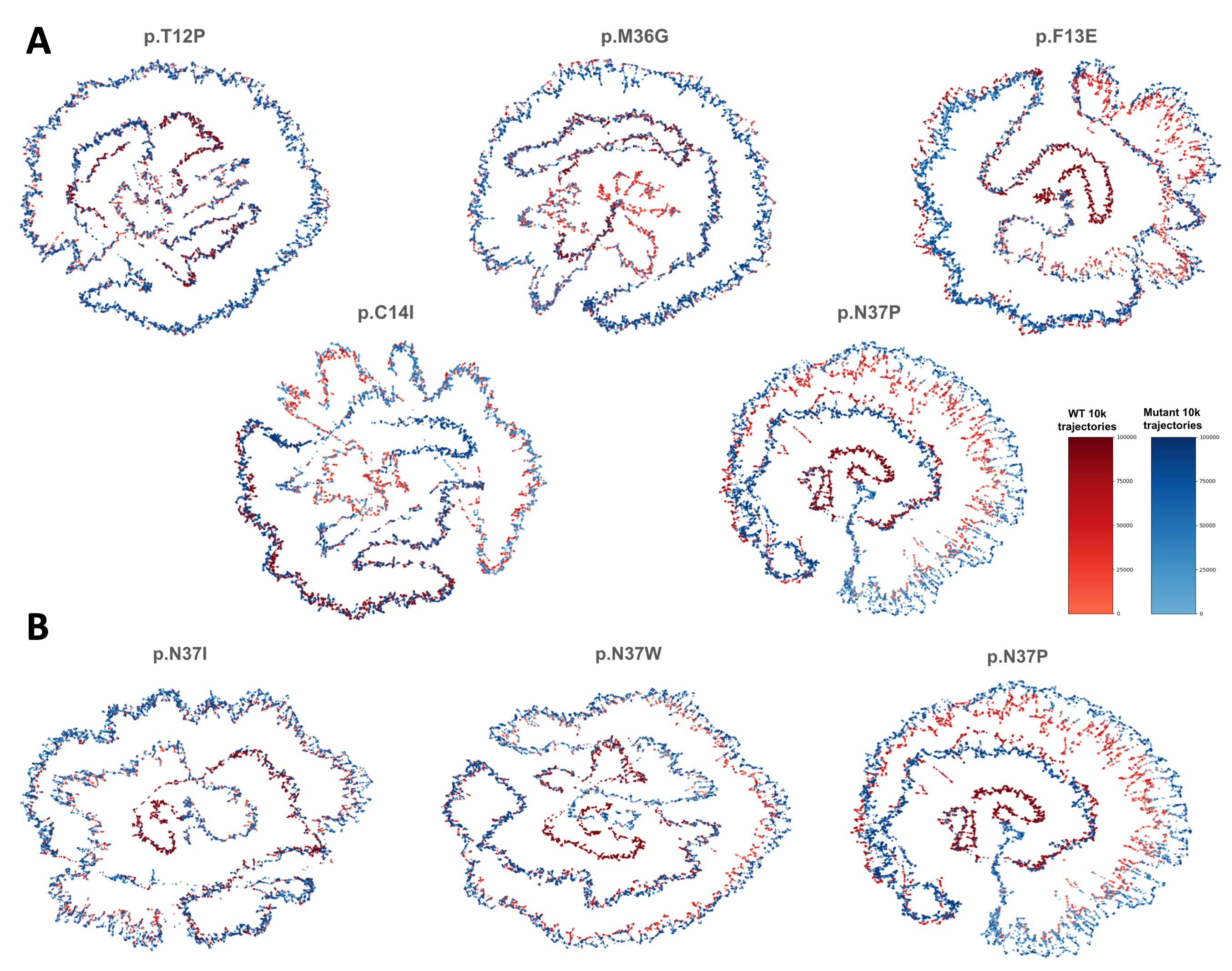
Figure 7: Analysis of MD trajectories of Protein Kinase C mutants using latent representations obtained by ProtSCAPE. (A) PHATE plots of wild-type (WT) and mutant (M) latent representations. We observe that the latent representations of the mutant trajectories largely overlaps with the wild-type trajectory. (B) We analyze the latent trajectories of progressively dissimilar substitutions to residue 37. Increasing dissimilarity results in more deviations from the wild-type trajectory in the latent space.

J Proofs

Before we can prove Theorem B.1 and B.2, we must introduce some notation and prove an auxiliary Theorem. In Section J.1, we will introduce a symmetric diffusion matrix $T$ as well as wavelets constructed from this symmetric diffusion operator. Then, in Section J.2, we will prove Theorem J.2.1 which is the analog of Theorem B.1, but for these symmetric, $T$-diffusion wavelets. We will then complete the proofs of Theorems B.1 and B.2 in Sections J.3 and J.4. Lastly, we will prove an two auxiliary lemmas in Section J.5 and Section J.6.

J.1 The symmetric diffusion operator and associated $T$-diffusion wavelets

Let $L_{N}\coloneqq I-D^{-1/2}AD^{-1/2}$ be the symmetric normalized graph Laplacian. Since we assume $G$ is connected, it is known [34] that $L_{N}$ admits an orthonormal basis of eigenvectors $\mathbf{v}_{1},\ldots,\mathbf{v}_{n}$, with $L_{N}\mathbf{v}_{i}=\omega_{i}\mathbf{v_{i}},$ $0=\omega_{1}<\omega_{2}\leq\ldots\leq\omega_{n}$.

We define the symmetric diffusion operator

$$T\coloneqq D^{-1/2}PD^{1/2}=\frac{1}{2}\left(I+D^{-1/2}AD^{-1/2}\right),$$

and note that we may write

$$T=I-\frac{1}{2}L_{N}.$$

This implies that $T$ has the same eigenvectors as $L_{N}$ and that

$$T\mathbf{v}_{i}=\lambda_{i}\mathbf{v_{i}},\quad\lambda_{i}=1-\frac{1}{2}\omega_{i}.$$

In particular, we have

$$1=\lambda_{1}>\lambda_{2}\geq\ldots\geq\lambda_{n}\geq 0,$$ (4)

where the final inequality uses the fact that the eigenvalues of $L_{N}$ lie between $0$ and $2$, (see, e.g., Lemma 1.7 of [34]).

Given $T$, we next consider an alternate version of the wavelet transform, defined by $\widetilde{\Psi}^{(T)}_{0}=I-T^{t_{1}}$ and

$$\widetilde{\Psi}^{(T)}_{j}=T^{t_{j}}-T^{t_{j+1}},\text{ for }1\leq j\leq J,$$ (5)

which we will refer to as the $T$-diffusion wavelets. (Note that we are using the same scales $t_{j}$ for both $\widetilde{\Psi}_{j}$ and $\widetilde{\Psi}^{(T)}_{j}$.)

J.2 Stability for the $T$-diffusion wavelets

In this section, we will prove the following theorem which is the analog of Theorem B.1, but for the $T$-diffusion wavelets.

Theorem J.2.1.

Let $G^{\prime}=(V^{\prime},E^{\prime})$ be a perturbed version of $G=(V,E)$ and let $T^{\prime}$ be the analog of $T$ but on $G^{\prime}$. Let $\widetilde{\Psi}^{(T)}_{j}$ denote the $T$-diffusion wavelets defined as in (5), and let $(\widetilde{\Psi}^{(T)}_{j})^{\prime}$ denote the analog of $\widetilde{\Psi}^{(T)}_{j}$ on $G^{\prime}$. Then, for all $\mathbf{x}\in\mathbb{R}^{n}$, we have

$$\sum_{j=0}^{J}\|\widetilde{\Psi_{j}}^{(T)}\mathbf{x}-(\widetilde{\Psi_{j}}^{(T)})^{\prime}\mathbf{x}\|_{2}^{2}\leq C_{\lambda_{2}*}\|T-T^{\prime}\|\|\mathbf{x}\|_{2}^{2},$$ (6)

where $C_{\lambda_{2}^{*}}$ is a constant depending only on $\lambda_{2}^{*}$.

Proof.

Let $\mathbf{v}=\mathbf{v}_{1}$ and $\mathbf{v}^{\prime}=\mathbf{v}_{1}^{\prime}$ denote the lead eigenvector of $T$ and $T^{\prime}$. Let $\bar{T}\coloneqq T-\mathbf{v}\mathbf{v}^{T}$ and $\bar{T}^{\prime}\coloneqq T^{\prime}-\mathbf{v}^{\prime}(\mathbf{v}^{\prime})^{T}$.

By construction, the $\ell^{2}$ operator norms of $\bar{T}$ and $\bar{T}^{\prime}$ are given by $\|\bar{T}\|=\lambda_{2}$ and $\|\bar{T}^{\prime}\|=\lambda^{\prime}_{2}$. Let $\lambda_{2}^{*}=\max\{\lambda_{2},\lambda_{2}^{\prime}\}$ denote the larger of these two operator norms. Note that $\lambda_{2}^{*}<1$ by (4).

Since $\mathbf{v}_{1},\ldots,\mathbf{v}_{n}$ forms an orthonormal basis, we observe that, for any $k\geq 1$, we have

$$T^{k}=(\mathbf{v}\mathbf{v}^{T}+\bar{T})^{k}=\mathbf{v}\mathbf{v}^{T}+\bar{T}^{k}.$$

This implies that $\widetilde{\Psi}^{(T)}_{0}=I-\mathbf{v}\mathbf{v}^{T}-\bar{T}^{t_{1}}$ and

$$\widetilde{\Psi}^{(T)}_{j}=T^{t_{j}}-T^{t_{j+1}}=\bar{T}^{t_{j}}-\bar{T}^{t_{j+1}}$$

for $1\leq j\leq J+1$. Thus, we have

$$\sum_{j=0}^{J}\|\widetilde{\Psi_{j}}^{(T)}\mathbf{x}-(\widetilde{\Psi_{j}}^{(T)})^{\prime}\mathbf{x}\|_{2}^{2}$$

$$= \left(\|\mathbf{v}\mathbf{v}^{T}-\mathbf{v}^{\prime}(\mathbf{v}^{\prime})^{T}-(\bar{T}^{t_{1}}-(\bar{T}^{\prime})^{t_{1}}\|^{2}+\sum_{j=1}^{J}\|(\bar{T}^{t_{j}}-\bar{T}^{t_{j+1}})-((\bar{T}^{\prime})^{t_{j}}-(\bar{T}^{\prime})^{t_{j+1}})\|^{2}\right)\|\mathbf{x}\|_{2}^{2}$$

$$\leq 4\left(\|\mathbf{v}\mathbf{v}^{T}-\mathbf{v}^{\prime}(\mathbf{v}^{\prime})^{T}\|^{2}+\sum_{j=1}^{J+1}\left\|\bar{T}^{t_{j}}-\left(\bar{T}^{\prime}\right)^{t_{j}}\right\|^{2}\right)\|\mathbf{x}\|^{2}_{2},$$ (7)

where we use the fact that

$$(\bar{T}^{t_{j}}-\bar{T}^{t_{j+1}})-((\bar{T}^{\prime})^{t_{j}}-(\bar{T}^{\prime})^{t_{j+1}})=(\bar{T}^{t_{j}}-(\bar{T}^{\prime})^{t_{j}})-(\bar{T}^{t_{j+1}}-(\bar{T}^{\prime})^{t_{j+1}}),$$

the inequality $\|A-B\|^{2}\leq 2(\|A\|^{2}+\|B\|^{2})$ and observation that each of the powers $t_{j}$ in (7) appears at most twice in the sum in the previous line (once as the $j$ term and once as $j+1$ term).

To bound $\sum_{j=1}^{J+1}\left\|\bar{T}^{t_{j}}-\left(\bar{T}^{\prime}\right)^{t_{j}}\right\|^{2}$, we will use the following lemma which is a variant of Lemma SM12.1 of Perlmutter et al. [28] (see also Lemma 7 of [35] and Equation 23 of Gama et al. [11]). For a proof, please see Section J.6.

Lemma J.2.2.

$$\sum_{j=1}^{J+1}\left\|\bar{T}^{t_{j}}-\left(\bar{T}^{\prime}\right)^{t_{j}}\right\|^{2}\leq C_{\lambda_{2}^{*}}\|\bar{T}-\bar{T}^{\prime}\|^{2},$$

where $C_{\lambda_{2}^{*}}>0$ is a constant depending only on $\lambda_{2}*$.

The triangle inequality implies that

$$\|\bar{T}-\bar{T}^{\prime}\|\leq\|T-T^{\prime}\|+\|\mathbf{v}\mathbf{v}^{T}-\mathbf{v}^{\prime}(\mathbf{v}^{\prime})^{T}\|,$$

and so combining (7) with (J.2.2) yields

$$\sum_{j=0}^{J}\|\widetilde{\Psi_{j}}^{(T)}\mathbf{x}-(\widetilde{\Psi_{j}}^{(T)})^{\prime}\mathbf{x}\|_{2}^{2} \leq 4\left(\|\mathbf{v}\mathbf{v}^{T}-\mathbf{v}^{\prime}(\mathbf{v}^{\prime})^{T}\|^{2}+\sum_{j=1}^{J+1}\left\|\bar{T}^{t_{j}}-\left(\bar{T}^{\prime}\right)^{t_{j}}\right\|^{2}\right)\|\mathbf{x}\|^{2}_{2}$$

$$\leq C_{\lambda_{2}^{*}}(\|\mathbf{v}\mathbf{v}^{T}-\mathbf{v}^{\prime}(\mathbf{v}^{\prime})^{T}\|^{2}+\|T-T^{\prime}\|^{2})\|\mathbf{x}\|_{2}^{2}.$$ (8)

Next, using the fact that $\mathbf{v}$ has unit norm, one may verify that $\|\mathbf{v}\mathbf{v}^{T}-\mathbf{v}^{\prime}(\mathbf{v}^{\prime})^{T}\|\leq 2\|\mathbf{v}-\mathbf{v}^{\prime}\|_{2}$ since, for all $\mathbf{x}$, we have

$$\left\|(\mathbf{v}\mathbf{v}^{T}-\mathbf{v}^{\prime}(\mathbf{v}^{\prime})^{T})\mathbf{x}\right\|_{2} \leq\left\|\mathbf{v}(\mathbf{v}-\mathbf{v}^{\prime})^{T}\mathbf{x}\right\|_{2}+\left\|(\mathbf{v}-\mathbf{v}^{\prime})(\mathbf{v}^{\prime})^{T}\mathbf{x}\right\|_{2}$$

$$\leq\|\mathbf{v}\|_{2}\left\|\mathbf{v}-\mathbf{v}^{\prime}\right\|_{2}\|\mathbf{x}\|_{2}+\left\|\mathbf{v}-\mathbf{v}^{\prime}\right\|_{2}\|\mathbf{v}^{\prime}\|_{2}\|\mathbf{x}\|_{2}$$

$$\leq 2\left\|\mathbf{v}-\mathbf{v}^{\prime}\right\|_{2}\|\mathbf{x}\|_{2}.$$

Lemma SM10.2 of Perlmutter et al. [28] shows that

$$\|\mathbf{v}-\mathbf{v}^{\prime}\|_{2}^{2}\leq C_{\lambda_{2}^{*}}\|T-T^{\prime}\|.$$

Combining this with (8), we have

$$\sum_{j=0}^{J}\|\widetilde{\Psi_{j}}^{(T)}\mathbf{x}-(\widetilde{\Psi_{j}}^{(T)})^{\prime}\mathbf{x}\|_{2}^{2} \leq C_{\lambda_{2}^{*}}(\|\mathbf{v}\mathbf{v}^{T}-\mathbf{v}^{\prime}(\mathbf{v}^{\prime})^{T}\|^{2}+\|T-T^{\prime}\|^{2})\|\mathbf{x}\|_{2}^{2}$$

$$\leq C_{\lambda_{2}*}(\|T-T^{\prime}\|+\|T-T^{\prime}\|^{2})\|\mathbf{x}\|_{2}^{2}.$$

Finally, we note that

$$\|T-T^{\prime}\|\leq\|T\|+\|T^{\prime}\|\leq\lambda_{2}+\lambda_{2}^{\prime}<2,$$

which implies

$$\sum_{j=0}^{J}\|\widetilde{\Psi_{j}}^{(T)}\mathbf{x}-(\widetilde{\Psi_{j}}^{(T)})^{\prime}\mathbf{x}\|_{2}^{2}\leq C_{\lambda_{2}*}\|T-T^{\prime}\|\|\mathbf{x}\|_{2}^{2},$$ (9)

and thus completes the proof. ∎

J.3 The Proof of Theorem B.1

To complete the proof of Theorem B.1 we recall the following result which is a simplified version of Perlmutter et al. [28], Theorem 4.3 (where here we simplify the result by restricting to the case where each $r_{j}$ is the appropriate polynomial and assuming that $M=D^{-1/2}$, which is equivalent to assuming that $K=P$).

In order to state this result we briefly introduce some notation. Let $\tilde{\mathcal{W}}_{J}=\{\widetilde{\Psi_{j}}\}_{j=0}^{J}$, let $\tilde{\mathcal{W}}^{\prime}_{J}=\{(\widetilde{\Psi_{j}})^{\prime}\}_{j=0}^{J}$, and let $\tilde{\mathcal{W}}_{J}-\tilde{\mathcal{W}}^{\prime}_{J}=\{\widetilde{\Psi_{j}}-(\widetilde{\Psi_{j}})^{\prime}\}_{j=0}^{J}$. Let $\|\tilde{\mathcal{W}}_{J}-\tilde{\mathcal{W}}^{\prime}_{J}\}_{j=0}^{J}\|_{D^{-1/2}}$ denote the operator norm of $\tilde{\mathcal{W}}_{J}-\tilde{\mathcal{W}}^{\prime}_{J}$ on the weighted inner product space corresponding to $\|\cdot\|_{D^{-1/2}}$ given by

$$\|\tilde{\mathcal{W}}_{J}-\tilde{\mathcal{W}}^{\prime}_{J}\|_{D^{-1/2}}\coloneqq\sup_{\|\mathbf{x}\|_{D^{-1/2}}=1}\left(\sum_{j=0}^{J}\|\widetilde{\Psi_{j}}\mathbf{x}-(\widetilde{\Psi_{j}})^{\prime}\mathbf{x}\|_{D^{-1/2}}^{2}\right)^{1/2}.$$

Similarly, define

$$\|\tilde{\mathcal{W}}_{J}^{(T)}-(\tilde{\mathcal{W}}_{J}^{(T)})^{\prime}\|\coloneqq\sup_{\|\mathbf{x}\|_{2}=1}\left(\sum_{j=0}^{J}\|\widetilde{\Psi_{j}}^{(T)}\mathbf{x}-(\widetilde{\Psi_{j}}^{(T)})^{\prime}\mathbf{x}\|_{2}^{2}\right)^{1/2}.$$

We may now state our result.

Theorem J.3.1 (Special Case of Theorem 4.3 of Perlmutter et al. [28]).

$$\|\tilde{\mathcal{W}}_{J}-\tilde{\mathcal{W}}^{\prime}_{J}\|^{2}_{D^{-1/2}}\leq 6\left(\|\tilde{\mathcal{W}}_{J}^{(T)}-(\tilde{\mathcal{W}}_{J}^{(T)})^{\prime}\|^{2}+\kappa^{2}(\kappa+1)^{2}\right).$$ (10)

Remark J.3.2.

We do note that in order to apply Theorem 4.3 of Perlmutter et al. [28] we need to verify that each of the wavelet filter banks, when paired with an appropriate low-pass filter, form a non-expansive frame on the appropriate inner-product space (corresponding to the norm $\|\cdot\|_{D^{-1/2}}$ in the case of the wavelets constructed via $P$ and the standard $\ell^{2}$ inner-product space for the $T$-diffusion wavelets). For the $P$-diffusion wavelets, this follows immediately from Theorem 1 of Tong et al. [9]. For the $T$-diffusion wavelets, this may be established by repeating the proof of Tong et al. [9], Theorem 1, line by line, but replacing $D^{-1/2}$ with the identity in every step. (See also Proposition 2.2 of [28] which gives frame bounds for the $T$-diffusion wavelets in the case where the scales are chosen to be dyadic powers.)

Additionally, we need to recall the following result, which is a special case of Perlmutter et al. [28], Proposition 4.6 (whereas before we restrict to the case where $M=D^{-1/2}$).

Theorem J.3.3.

Special Case of Proposition 4.6 of Perlmutter et al. [28]

$$\|T-T^{\prime}\|\leq\kappa(1+R^{3})+R\|P-P^{\prime}\|_{D^{-1/2}},$$

where $\|T-T^{\prime}\|$ and $\|P-P^{\prime}\|_{D^{-1/2}}$ are the operator norms of the relevant matrices on the standard $\ell^{2}$ inner product space and the weighted inner-product space corresponding to $\|\cdot\|_{D^{-1/2}}$.

It is now straightforward to complete the proof.

The proof of Theorem B.1.

Combining Theorems J.2.1, J.3.1 and J.3.3 yields

$$\|\tilde{\mathcal{W}}_{J}-\tilde{\mathcal{W}}^{\prime}_{J}\|^{2}_{D^{-1/2}} \leq 6\left(\|\tilde{\mathcal{W}}_{J}^{(T)}-(\tilde{\mathcal{W}}_{J}^{(T)})\|^{2}+\kappa^{2}(\kappa+1)^{2}\right)$$

$$\leq C_{\lambda_{2}*}\left(\|T-T^{\prime}\|+\kappa^{2}(\kappa+1)^{2}\right)$$

$$\leq C_{\lambda_{2}*}\left(\kappa(1+R^{3})+R\|P-P^{\prime}\|_{D^{-1/2}}+\kappa^{2}(\kappa+1)^{2}\right)$$

as desired. ∎

J.4 The Proof of Theorem B.2

To prove Theorem B.2, we will need the following lemma. For a proof, please see Section J.5.

Lemma J.4.1.

For any $\ell\geq 1$, we have

$$\sum_{0\leq j_{1},\ldots,j_{\ell}\leq J}\|\widetilde{U}[j_{1},\ldots,j_{\ell}]\mathbf{x}\|^{2}_{D^{-1/2}}\leq\|\mathbf{x}\|_{D^{-1/2}}.$$

Now, we will prove Corollary B.2.

Proof.

Let

$$\mathcal{C}\coloneqq\sup_{\|\mathbf{x}\|_{D^{-1/2}}=1}\left(\sum_{j=0}^{J}\|(\widetilde{\Psi_{j}})^{\prime}\mathbf{x}\|_{D^{-1/2}}^{2}\right)^{1/2}$$

denote the operator norm of the perturbed wavelets with respect to the norm $\|\cdot\|_{D^{-1/2}}$ and let

$$\mathcal{A}\coloneqq\|\tilde{\mathcal{W}}_{J}-\tilde{\mathcal{W}}^{\prime}_{J}\|_{D^{-1/2}}$$

denote the operator norm of the difference between the $\tilde{\mathcal{W}}_{J}$ and the perturbed-graph wavelets $\tilde{\mathcal{W}}^{\prime}_{J}$.

We will show that, for all $\ell\geq 1$, we have

$$\sum_{0\leq j_{1},\ldots,j_{\ell}\leq J}\|\widetilde{U}[j_{1},\ldots,j_{\ell}]\mathbf{x}-\widetilde{U}^{\prime}[j_{1},\ldots,j_{\ell}]\mathbf{x}\|^{2}_{D^{-1/2}}\leq\mathcal{A}^{2}\left(\sum_{k=0}^{\ell-1}\mathcal{C}^{k}\right)^{2}\|\mathbf{x}\|^{2}_{D^{-1/2}}.$$ (11)

Let $t_{\ell}\coloneqq\left(\sum_{0\leq j_{1},\ldots,j_{\ell}\leq J}\|\widetilde{U}[j_{1},\ldots,j_{\ell}]\mathbf{x}-\widetilde{U}^{\prime}[j_{1},\ldots,j_{\ell}]\mathbf{x}\|^{2}_{D^{-1/2}}\right)^{1/2}$. Since the modulus operator $M$ is non-expansive (i.e., $\|M(\mathbf{x}-\mathbf{y})\|_{D^{-1/2}}\leq\|\mathbf{x}-\mathbf{y}\|_{D^{-1/2}}$), it follows that $t_{1}\leq\mathcal{A}\|\mathbf{x}\|_{D^{-1/2}}$ which proves the base case.

Now, suppose by induction that (11) holds for $\ell$. Then,

$$t_{\ell+1} =\left(\sum_{0\leq j_{1},\ldots,j_{\ell},j_{\ell+1}\leq J}\|\widetilde{U}[j_{1},\ldots,j_{\ell+1}]\mathbf{x}-\widetilde{U}^{\prime}[j_{1},\ldots,j_{\ell+1}]\mathbf{x}\|^{2}_{D^{-1/2}}\right)^{1/2}$$

$$=\left(\sum_{0\leq j_{1},\ldots,j_{\ell},j_{\ell+1}\leq J}\|M\widetilde{\Psi}_{j_{\ell+1}}\ldots M\widetilde{\Psi}_{j_{1}}\mathbf{x}-M\widetilde{\Psi}^{\prime}_{j_{\ell+1}}\ldots M\widetilde{\Psi}^{\prime}_{j_{1}}\mathbf{x}\|^{2}_{D^{-1/2}}\right)$$

$$\leq\left(\sum_{0\leq j_{1},\ldots,j_{\ell},j_{\ell+1}\leq J}\|(\widetilde{\Psi}_{j_{\ell+1}}-\widetilde{\Psi}_{j_{\ell+1}}^{\prime})M\widetilde{\Psi}_{j_{\ell}}\ldots M\widetilde{\Psi}_{j_{1}}\mathbf{x}\|^{2}_{D^{-1/2}}\right)^{1/2}$$

$$\quad+\left(\sum_{0\leq j_{1},\ldots,j_{\ell},j_{\ell+1}\leq J}\|\widetilde{\Psi}^{\prime}_{j_{\ell+1}}(M\widetilde{\Psi}_{j_{\ell}}\ldots M\widetilde{\Psi}_{j_{1}}\mathbf{x}-M\widetilde{\Psi}^{\prime}_{j_{\ell}}\ldots M\widetilde{\Psi}^{\prime}_{j_{1}}\mathbf{x})\|^{2}_{D^{-1/2}}\right)^{1/2}$$

$$\leq\mathcal{A}\left(\sum_{0\leq j_{1},\ldots,j_{\ell}\leq J}\|M\widetilde{\Psi}_{j_{\ell}}\ldots M\widetilde{\Psi}_{j_{1}}\mathbf{x}\|^{2}_{D^{-1/2}}\right)^{1/2}$$

$$\quad+\mathcal{C}\left(\sum_{0\leq j_{1},\ldots,j_{\ell}\leq J}\|(M\widetilde{\Psi}_{j_{\ell}}\ldots M\widetilde{\Psi}_{j_{1}}\mathbf{x}-M\widetilde{\Psi}^{\prime}_{j_{\ell}}\ldots M\widetilde{\Psi}^{\prime}_{j_{1}}\mathbf{x})\|^{2}_{D^{-1/2}}\right)^{1/2}$$

$$\leq\mathcal{A}\|\mathbf{x}\|_{D^{-1/2}}+t_{\ell}\mathcal{C},$$

where in the final inequality we use Lemma J.4.1. By the inductive hypothesis, we have

$$t_{\ell}\leq\mathcal{A}\sum_{k=0}^{\ell-1}\mathcal{C}^{k}\|\mathbf{x}\|_{D^{-1/2}}.$$

Therefore,

$$t_{\ell+1}\leq\mathcal{A}\|\mathbf{x}\|_{D^{-1/2}}+\mathcal{A}\sum_{k=0}^{\ell-1}\mathcal{C}^{k+1}\|\mathbf{x}\|_{D^{-1/2}}=\mathcal{A}\sum_{k=0}^{\ell}\mathcal{C}^{k}\|\mathbf{x}\|_{D^{-1/2}}.$$

Squaring both sides yields (11). Proposition 4.10 of Perlmutter et al. [28] implies that $\mathcal{C}=R^{2}$. Thus, we have

$$\sum_{0\leq j_{1},\ldots,j_{\ell}\leq J}\|\widetilde{U}[j_{1},\ldots,j_{\ell}]\mathbf{x}-\widetilde{U}^{\prime}[j_{1},\ldots,j_{\ell}]\mathbf{x}\|^{2}_{D^{-1/2}}\leq\mathcal{A}^{2}\left(\sum_{k=0}^{\ell-1}R^{2k}\right)^{2}\|\mathbf{x}\|^{2}_{D^{-1/2}}.$$ (12)

∎

J.5 The Proof of Lemma J.4.1

Proof.

First, we note using the fact that the modulus operator $M$ is non-expansive, that

$$\left(\sum_{j=0}^{J}\|(\widetilde{\Psi_{j}})\mathbf{x}\|_{D^{-1/2}}^{2}\right)^{1/2}\leq\|\mathbf{x}\|_{D^{-1/2}}$$

by Theorem 1 of Tong et al. [9], which proves the claim for $\ell=1$.

Now, assuming by induction that the claim holds for $\ell$, we note that

$$\sum_{0\leq j_{1},\ldots,j_{\ell},j_{\ell+1}\leq J}\|\widetilde{U}[j_{1},\ldots,j_{\ell},j_{\ell+1}]\mathbf{x}\|^{2}_{D^{-1/2}} =\sum_{0\leq j_{1},\ldots,j_{\ell},j_{\ell+1}\leq J}\|M\widetilde{\Psi}_{j_{\ell+1}}\ldots M\widetilde{\Psi}_{j_{1}}\mathbf{x}\|^{2}_{D^{-1/2}}$$

$$=\sum_{0\leq j_{1},\ldots,j_{\ell}\leq J}\left(\sum_{0\leq j_{\ell+1}\leq J}\|M\widetilde{\Psi}_{j_{\ell+1}}\ldots M\widetilde{\Psi}_{j_{1}}\mathbf{x}\|^{2}_{D^{-1/2}}\right)$$

$$\leq\sum_{0\leq j_{1},\ldots,j_{\ell}\leq J}\|M\widetilde{\Psi}_{j_{\ell}}\ldots M\widetilde{\Psi}_{j_{1}}\mathbf{x}\|^{2}_{D^{-1/2}}$$

$$\leq\|\mathbf{x}\|_{D^{-1/2}}$$

again using Theorem 1 of [9] as well as the inductive hypothesis.

∎

J.6 The proof of Lemma J.2.2

Proof.

For $0\leq t\leq 1$, $1\leq j\leq J+1$, let

$$H_{j}(t)=\left(t\bar{T}+(1-t)\bar{T}^{\prime}\right)^{t_{j}}.$$

Then,

$$\|\bar{T}^{t_{j}}-\left(\bar{T}^{\prime}\right)^{t_{j}}\|=\|H_{j}(1)-H_{j}(0)\|\leq\int_{0}^{1}\|\partial_{t}H_{j}(t)\|dt\leq\sup_{0\leq t\leq 1}\|\partial_{t}H_{j}(t)\|.$$

One may compute

$$\partial_{t}H_{j}(t)=\sum_{\ell=0}^{t_{j}-1}(t\bar{T}^{\prime}+(1-t)\bar{T})^{\ell}(\bar{T}-\bar{T}^{\prime})(t\bar{T}^{\prime}+(1-t)\bar{T})^{t_{j}-\ell-1}.$$

Since $\|\bar{T}\|,\|\bar{T}^{\prime}\|\leq\lambda_{2}^{*}$, this implies

$$\sup_{0\leq t\leq 1}\|\partial_{t}H_{j}(t)\|\leq t_{j}(\lambda_{2}^{*})^{t_{j}-1}\|\bar{T}-\bar{T}^{\prime}\|.$$

Therefore,

$$\sum_{j=1}^{J+1}\left\|\bar{T}^{t_{j}}-\left(\bar{T}^{\prime}\right)^{t_{j}}\right\|^{2} \leq\|\bar{T}-\bar{T}^{\prime}\|^{2}\sum_{j=1}^{J+1}t_{j}^{2}(\lambda_{2}^{*})^{2t^{j}-2}$$

$$\leq\|\bar{T}-\bar{T}^{\prime}\|^{2}(\lambda_{2}^{*})^{-2}\sum_{k=1}^{\infty}k^{2}(\lambda_{2}^{*})^{k}$$

$$\eqqcolon C_{\lambda_{2}^{*}}\|\bar{T}-\bar{T}^{\prime}\|^{2},$$

as desired. (The fact the series converges follows from the fact that $\lambda_{2}^{*}<1.$ In the case where $\lambda_{2}^{*}=0$, then series is zero and we can omit the term which includes a $(\lambda_{2}^{*})^{-2}$ and instead choose $C_{\lambda_{2}^{*}}$ to be any positive constant.) ∎

References

- Eisenmesser et al. [2005] Elan Z. Eisenmesser, Oscar Millet, Wladimir Labeikovsky, Dmitry M. Korzhnev, Magnus Wolf-Watz, Daryl A. Bosco, Jack J. Skalicky, Lewis E. Kay, and Dorothee Kern. Intrinsic dynamics of an enzyme underlies catalysis. Nature, 438(7064):117–121, 2005.
- Wolf-Watz et al. [2004] Magnus Wolf-Watz, Vu Thai, Katherine Henzler-Wildman, Georgia Hadjipavlou, Elan Z Eisenmesser, and Dorothee Kern. Linkage between dynamics and catalysis in a thermophilic-mesophilic enzyme pair. Nature Structural & Molecular Biology, 11(10):945–949, 2004.
- Ma and Karplus [1998] Jianpeng Ma and Martin Karplus. The allosteric mechanism of the chaperonin groel: A dynamic analysis. Proceedings of the National Academy of Sciences, 95(15):8502–8507, 1998.
- Karplus and Kuriyan [2005] M. Karplus and J. Kuriyan. Molecular dynamics and protein function. Proceedings of the National Academy of Sciences, 102(19):6679–6685, 2005.
- Lisi et al. [2017] George P. Lisi, Kyle W. East, Victor S. Batista, and J. Patrick Loria. Altering the allosteric pathway in IGPS suppresses millisecond motions and catalytic activity. Proceedings of the National Academy of Sciences, 114(17):E3414–E3423, 2017.
- Vakser [2020] Ilya A Vakser. Challenges in protein docking. Current Opinion in Structural Biology, 64:160–165, 2020. ISSN 0959-440X. Biophysical and Computational Methods - Cryo EM.
- Orozco [2014] Modesto Orozco. A theoretical view of protein dynamics. Chem. Soc. Rev., 43:5051–5066, 2014.
- Lindorff-Larsen et al. [2011] Kresten Lindorff-Larsen, Stefano Piana, Ron O. Dror, and David E. Shaw. How fast-folding proteins fold. Science, 334(6055):517–520, 2011.
- Tong et al. [2022] Alexander Tong, Frederik Wenkel, Dhananjay Bhaskar, Kincaid Macdonald, Jackson Grady, Michael Perlmutter, Smita Krishnaswamy, and Guy Wolf. Learnable filters for geometric scattering modules. arXiv preprint arXiv:2208.07458, 2022.
- Gao et al. [2019] F. Gao, G. Wolf, and M. Hirn. Geometric scattering for graph data analysis. In Proc. of ICML, 2019.
- Gama et al. [2019] F. Gama, A. Ribeiro, and J. Bruna. Diffusion scattering transforms on graphs. In Proc. of ICLR, 2019.
- Zou and Lerman [2019] D. Zou and G. Lerman. Graph convolutional neural networks via scattering. Appl. Comp. Harm. Anal., 2019.
- Vander Meersche et al. [2024] Yann Vander Meersche, Gabriel Cretin, Aria Gheeraert, Jean-Christophe Gelly, and Tatiana Galochkina. Atlas: protein flexibility description from atomistic molecular dynamics simulations. Nucleic Acids Research, 52(D1):D384–D392, 2024.
- Bertrand et al. [1997] J A Bertrand, G Auger, E Fanchon, L Martin, D Blanot, J van Heijenoort, and O Dideberg. Crystal structure of UDP-N-acetylmuramoyl-L-alanine:D-glutamate ligase from escherichia coli. EMBO J., 16(12):3416–3425, June 1997.
- Degiacomi [2019] Matteo T Degiacomi. Coupling molecular dynamics and deep learning to mine protein conformational space. Structure, 27(6):1034–1040.e3, June 2019.
- Bertrand et al. [1999] J A Bertrand, G Auger, L Martin, E Fanchon, D Blanot, D Le Beller, J van Heijenoort, and O Dideberg. Determination of the MurD mechanism through crystallographic analysis of enzyme complexes. J. Mol. Biol., 289(3):579–590, June 1999.
- Bertrand et al. [2000] J A Bertrand, E Fanchon, L Martin, L Chantalat, G Auger, D Blanot, J van Heijenoort, and O Dideberg. “open” structures of MurD: domain movements and structural similarities with folylpolyglutamate synthetase. J. Mol. Biol., 301(5):1257–1266, September 2000.
- Šink et al. [2016] Roman Šink, Miha Kotnik, Anamarija Zega, Hélène Barreteau, Stanislav Gobec, Didier Blanot, Andréa Dessen, and Carlos Contreras-Martel. Crystallographic study of peptidoglycan biosynthesis enzyme MurD: Domain movement revisited. PLoS One, 11(3):e0152075, March 2016.
- Jumper et al. [2021] John Jumper, Richard Evans, Alexander Pritzel, Tim Green, Michael Figurnov, Olaf Ronneberger, Kathryn Tunyasuvunakool, Russ Bates, Augustin Žídek, Anna Potapenko, et al. Highly accurate protein structure prediction with alphafold. Nature, 596(7873):583–589, 2021.
- Baek et al. [2021] Minkyung Baek, Frank DiMaio, Ivan Anishchenko, Justas Dauparas, Sergey Ovchinnikov, Gyu Rie Lee, Jue Wang, Qian Cong, Lisa N Kinch, R Dustin Schaeffer, et al. Accurate prediction of protein structures and interactions using a three-track neural network. Science, 373(6557):871–876, 2021.
- Mirdita et al. [2022] Milot Mirdita, Konstantin Schütze, Yoshitaka Moriwaki, Lim Heo, Sergey Ovchinnikov, and Martin Steinegger. Colabfold: making protein folding accessible to all. Nature methods, 19(6):679–682, 2022.
- Abramson et al. [2024] Josh Abramson, Jonas Adler, Jack Dunger, Richard Evans, Tim Green, Alexander Pritzel, Olaf Ronneberger, Lindsay Willmore, Andrew J Ballard, Joshua Bambrick, et al. Accurate structure prediction of biomolecular interactions with alphafold 3. Nature, pages 1–3, 2024.
- Ramachandran et al. [1963] Ramachandran, Ramakrishnan, and Sasisekharan. Stereochemistry of polypeptide chain configurations.“. J. mol. Biol, 7:95–99, 1963.
- McGibbon et al. [2015] Robert T. McGibbon, Kyle A. Beauchamp, Matthew P. Harrigan, Christoph Klein, Jason M. Swails, Carlos X. Hernández, Christian R. Schwantes, Lee-Ping Wang, Thomas J. Lane, and Vijay S. Pande. Mdtraj: A modern open library for the analysis of molecular dynamics trajectories. Biophysical Journal, 109(8):1528 – 1532, 2015. doi: 10.1016/j.bpj.2015.08.015.
- Sun et al. [2006] Jimeng Sun, Dacheng Tao, and Christos Faloutsos. Beyond streams and graphs: dynamic tensor analysis. In Proceedings of the 12th ACM SIGKDD international conference on Knowledge discovery and data mining, pages 374–383, 2006.
- Ramanathan et al. [2011] Arvind Ramanathan, Ji Oh Yoo, and Christopher J. Langmead. On-the-Fly Identification of Conformational Substates from Molecular Dynamics Simulations. Journal of Chemical Theory and Computation, 7(3):778–789, March 2011. ISSN 1549-9618. doi: 10.1021/ct100531j. URL https://doi.org/10.1021/ct100531j. Publisher: American Chemical Society.
- Ramaswamy et al. [2021] Venkata K. Ramaswamy, Samuel C. Musson, Chris G. Willcocks, and Matteo T. Degiacomi. Deep Learning Protein Conformational Space with Convolutions and Latent Interpolations. Physical Review X, 11(1):011052, March 2021. doi: 10.1103/PhysRevX.11.011052. URL https://link.aps.org/doi/10.1103/PhysRevX.11.011052. Publisher: American Physical Society.
- Perlmutter et al. [2023] Michael Perlmutter, Alexander Tong, Feng Gao, Guy Wolf, and Matthew Hirn. Understanding graph neural networks with generalized geometric scattering transforms. SIAM Journal on Mathematics of Data Science, 5(4):873–898, 2023.
- Gama et al. [2020] Fernando Gama, Joan Bruna, and Alejandro Ribeiro. Stability properties of graph neural networks. IEEE Transactions on Signal Processing, 68:5680–5695, 2020.
- Moon et al. [2019] Kevin R Moon, David Van Dijk, Zheng Wang, Scott Gigante, Daniel B Burkhardt, William S Chen, Kristina Yim, Antonia van den Elzen, Matthew J Hirn, Ronald R Coifman, et al. Visualizing structure and transitions in high-dimensional biological data. Nature biotechnology, 37(12):1482–1492, 2019.
- Schrödinger, LLC [2015] Schrödinger, LLC. The PyMOL molecular graphics system, version 1.8. November 2015.
- Sneath [1966] P. H. A. Sneath. Relations between chemical structure and biological activity in peptides. Journal of Theoretical Biology, 12(2):157–195, November 1966. ISSN 0022-5193. doi: 10.1016/0022-5193(66)90112-3. URL https://www.sciencedirect.com/science/article/pii/0022519366901123.
- Abraham et al. [2024] Mark Abraham, Andrey Alekseenko, Vladimir Basov, Cathrine Bergh, Eliane Briand, Ania Brown, Mahesh Doijade, Giacomo Fiorin, Stefan Fleischmann, Sergey Gorelov, Gilles Gouaillardet, Alan Grey, M. Eric Irrgang, Farzaneh Jalalypour, Joe Jordan, Carsten Kutzner, Justin A. Lemkul, Magnus Lundborg, Pascal Merz, Vedran Miletic, Dmitry Morozov, Julien Nabet, Szilard Pall, Andrea Pasquadibisceglie, Michele Pellegrino, Hubert Santuz, Roland Schulz, Tatiana Shugaeva, Alexey Shvetsov, Alessandra Villa, Sebastian Wingbermuehle, Berk Hess, and Erik Lindahl. Gromacs 2024.2 manual. 2024. doi: 10.5281/ZENODO.11148638.
- Chung [1997] Fan RK Chung. Spectral graph theory, volume 92. American Mathematical Soc., 1997.
- Chew et al. [2024] Joyce Chew, Matthew Hirn, Smita Krishnaswamy, Deanna Needell, Michael Perlmutter, Holly Steach, Siddharth Viswanath, and Hau-Tieng Wu. Geometric scattering on measure spaces. Applied and Computational Harmonic Analysis, page 101635, 2024.