Efficient Circuit Wire Cutting Based on Commuting Groups
Abstract
Current quantum devices face challenges when dealing with large circuits due to error rates as circuit size and the number of qubits increase. The circuit wire-cutting technique addresses this issue by breaking down a large circuit into smaller, more manageable subcircuits. However, the exponential increase in the number of subcircuits and the complexity of reconstruction as more cuts are made poses a great practical challenge. Inspired by ancilla-assisted quantum process tomography and the MUBs-based grouping technique for simultaneous measurement, we propose a new approach that can reduce subcircuit running overhead. The approach first uses ancillary qubits to transform all quantum input initializations into quantum output measurements. These output measurements are then organized into commuting groups for the purpose of simultaneous measurement, based on MUBs-based grouping. This approach significantly reduces the number of necessary subcircuits as well as the total number of shots. Lastly, we provide numerical experiments to demonstrate the complexity reduction.
I Introduction
Recent advancements in quantum computing and quantum hardware have had a transformative impact on various sectors in industry and academia [1, 2]. Despite the potential of quantum computing, many-qubit technologies still face great hurdles such as the limited number of qubits and the low fidelity of the qubits. IBM’s creation of Condor, one of the world’s largest quantum computer systems with 1121 qubits [3], highlights the great advancements of quantum hardware during the past decade. However, these systems are still far from practical applications. John Preskill described such systems as Noisy Intermediate-Scale Quantum (NISQ) computers, emphasizing the significant work being done to improve qubit fidelity and increase qubit count [4, 5, 6, 7].
Given the constraints on the size of quantum hardware, how to effectively leverage the limited available quantum resources becomes a crucial problem. One promising approach is the quantum circuit cutting method, which divides a large quantum circuit into smaller circuit fragments that can be run independently on available quantum devices and the outputs of each fragments are combined classically. Empirical studies have shown that cutting a circuit helps reduce the impact of noise [8, 9] and can be used for error mitigation [10]. Additionally, research has focused on accurately accounting for statistical shot noise and adapting the approach to address specific challenges, such as combinatorial optimization [11]. Therefore, this technique offers considerable potential for overcoming numerous practical challenges in utilizing quantum hardware, especially in the NISQ era.
However, the success of circuit cutting techniques are significantly hampered by the fact that the runtime may increase exponentially with the number of cuts. Similar to quantum state tomography, circuit cutting involves classically monitoring all quantum degrees of freedom at the cut points, naturally leading to exponential blowup as the size of the quantum state grows. Efforts to reduce these costs include the implementation of randomized measurements [12, 13], classical sampling [14], golden circuit cutting points [15, 16], and variational optimization [17]. Nonetheless, the exponential growth in runtime is unlikely to vanish without imposing structural assumptions on the circuit. Alternatively, finding applications of circuit cutting that avoid the run time blowup issues, as demonstrated in [10], remains a question that is worth investigating.
The work introduced in this paper addresses the former issue of the exponential complexity of runtime. Our method is built mainly upon the following two simple observations:
Observation 1 (Initialization via Measurement Operator): Inspired by ancilla-assisted quantum process tomography [18, 19], we replace the states initialization at the front of the circuits by an equivalent procedure, which first entangles each input qubit with an ancilla qubit into a Bell state and then measures ancilla qubit on corresponding desired basis;
Observation 2 (Simultaneous Measurement in a Commuting Group): We utilize the well-known fact that observables within a commuting group—often referred to in the literature as a commuting family—can be diagonalized simultaneously. Therefore, measuring on any one operator provides the complete information of all the observables in the group.
Based on the observations above, we propose to replace quantum state initializations with measurements (Observation 1) by introducing additional ancilla qubits. Then, we employ simultaneous measurement (Observation 2) to efficiently measure all observables. Recall that the Pauli operators (or Pauli strings, which are the tensor products of Pauli matrices) provide a complete basis of observables on the Hilbert space of qubits. Thus, to obtain complete information for qubits, we must obtain measurement results from all Pauli operators. Partitioning these Pauli operators into groups can reduce the required measurements, thanks to simultaneous measurement. Therefore, a good partition is key to maximizing the benefits of simultaneous measurement.
Built on previous works in the framework of Mutually Unbiased Bases (MUBs) [20, 21, 22, 23, 24], Lawrence et al. [24] show that the optimal partition of Pauli operators is organizing them into commuting groups, each consisting of internally commuting observables. The existence of such optimal commuting operators partition implies, in the ideal case, polynomial improvements on the numbers of subcircuits a circuit cutting generates as well as the total number of shots required when measurement accuracy is taken into consideration. For realistic implementation, there are trade-offs: adding more ancilla qubits and introducing additional gates to the subcircuit. Our experimental results demonstrate strong evidence of polynomial savings in the number of shots.
The rest of the paper is organized as follows. Background on circuit cutting, MUBs-based grouping and simultaneous measurement are reviewed in Section II. We then discuss the methodology for converting initializations to measurements in Section III. Subsequently, we demonstrate our proposed method—combining techniques introduced in the previous sections—in Section IV and we analyze the advantages and trade-offs of our method in the subsequent Section V. Finally, we validate our theory and analysis with empirical evidence in Section VI and make conclusions in Section VII.
II Background
II-A Circuit Cutting
Circuit cutting is primarily classified into two methods: ’wire cutting’ and ’gate cutting’ [25, 26]. Circuit wire cutting can be further categorized into two types: with classical communication [27, 28, 29] and without classical communication [30, 31]. In this paper, we focus on circuit cutting without classical communication. Hence, when we refer to ’circuit cutting’, we are specifically discussing wire cutting without classical communication.
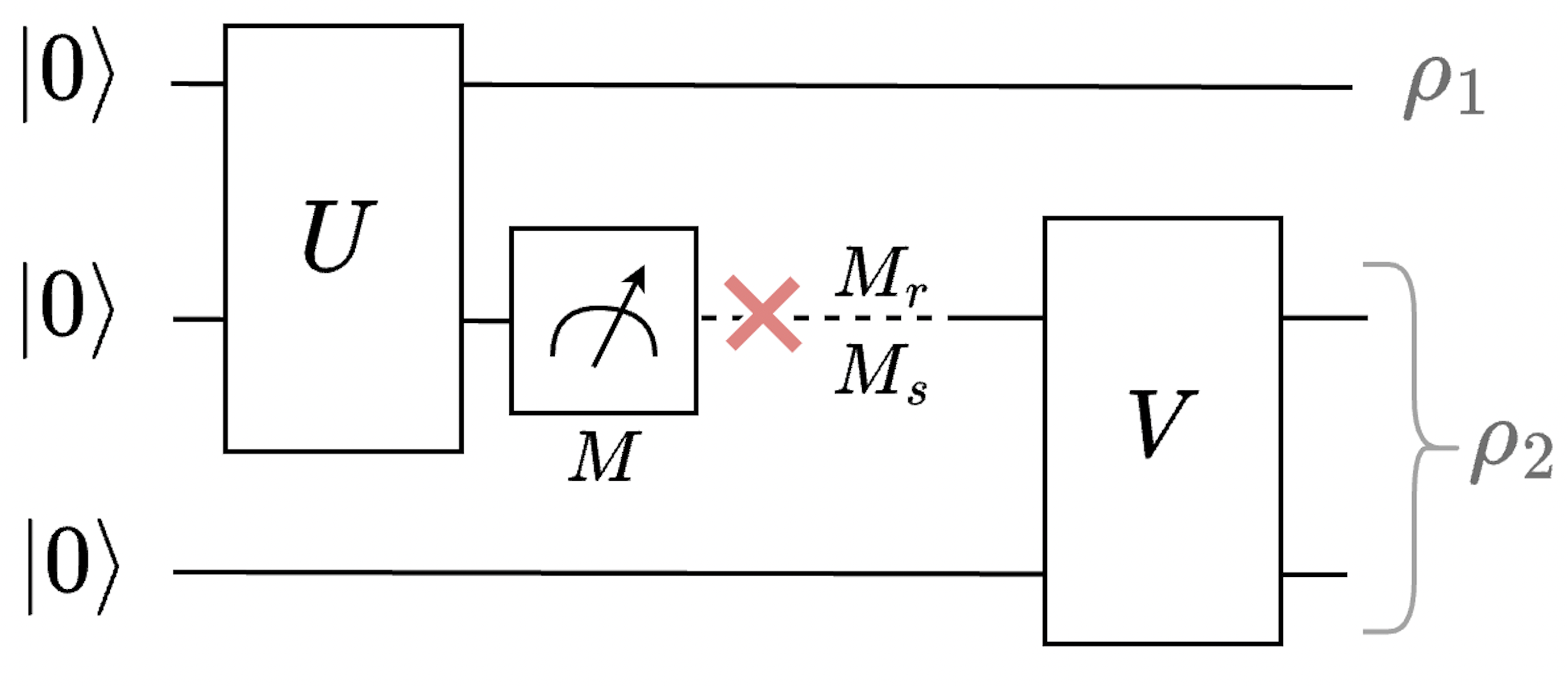
Let us start from a simple state of a three-qubit quantum circuit, as depicted in Fig. 1. The state of the circuit can be expressed as . Here, acts on the 1st and 2nd qubits, and acts on the 2nd and 3rd qubits. For simplicity, although it should be and , we use and to denote these operations respectively. The cut, marked as a red cross mark in Fig. 1, separates the circuit into two 2-qubit fragments associated with the unitary operations and respectively. As detailed in [30, 31], a single qubit’s state can be decomposed as
| (1) |
Following this decomposition, the example circuit can be represented as:
| (2) |
where and denotes the partial trace on the -th qubit. Denote the states for fragments and (parameterized by basis elements ) as
| (3) | ||||
| (4) |
the state of the circuit can be rewritten as the tensor product of states
| (5) |
Note that the partial trace operation in corresponds to a measurement, whereas the operator is used to indicate the initialization and for . Moreover, we adopt the terminology from Ref. [32] and view circuit fragments as quantum channels. Therefore, we will refer to parts of fragments as classical/quantum input/output; see Fig. 2 for an illustration.
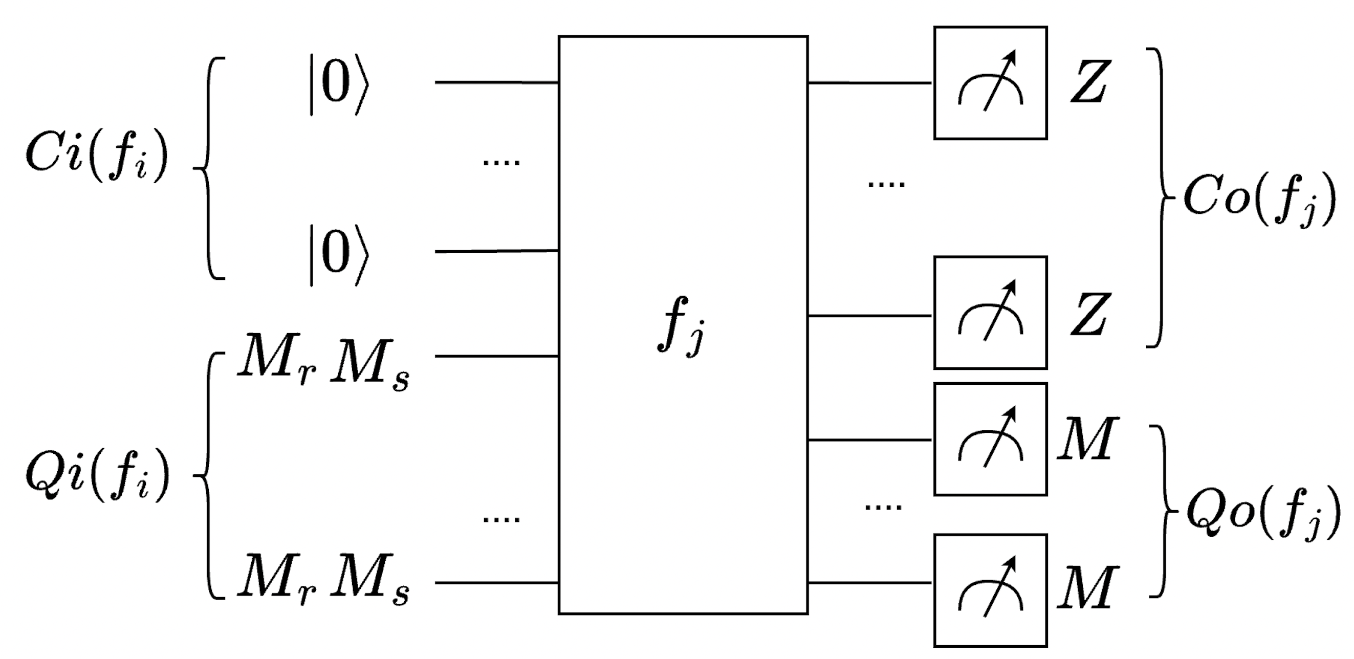
For a more general case involving cuts that produce fragments , we define , where and represent the quantum output and input observables, respectively. We denote the classical output state corresponding to fragment and operator by , and the unitary operator within the circuit corresponding to -th fragment (ignoring initializations and measurements) as . The fragment contains qubits, which comprise quantum input qubits, quantum output qubits, classical input qubits, and classical output qubits. and can be represented as a and length Pauli string. It is possible that , , , and could sometimes be zero; however, the relationship must be satisfied. For convenience, we denote the quantum input, quantum output, classical input, and classical output qubit index set for -th fragment as , , , and , respectively. For example, should contain qubit indices. By , we imply the tensor product of all qubits within the index set . Additionally, denotes the operation of taking the trace over all qubits indexed in . The subcircuit can be formally expressed as
| (6) |
where , the sum of the number of quantum input and output qubits. The final uncut circuit can be represented as
| (7) |
Note that the notation used in subsequent sections is derived from this section.
II-B MUBs-Based Grouping and Simultaneous Measurement
Simultaneous measurement is a technique that allows for the measurement of multiple observables in a circuit simultaneously, utilizing MUBs-based grouping. This is accomplished by organizing all observables into commuting groups, also known as commuting families in some literature. These groups comprise Pauli operators that commute with each other, allowing all observables within a group to be measured simultaneously in a single session. This approach can significantly reduce the number of measurements needed. It has been widely used in variational quantum eigensolver[33], quantum phase estimation [34], and classical shadow tomography [35]. We also want to simplify circuit cutting via simultaneous measurement.
Let us start with the definition of the commutator. The commutator of two elements and is defined
| (8) |
When , it indicates that and commute. In quantum mechanics, when Hermitian observables commute, it implies that they share a common set of eigenstates [36], [37]. Thus, by measuring this set of eigenstates, we can simultaneously obtain information for all members in the commuting group. In information science, mutually unbiased bases (MUBs) [20, 21, 22, 23, 24] guide the partitioning of -qubit Pauli operators into optimal commuting groups, known as ’MUBs-based grouping’. The optimal partition of , a set of Pauli operators, is groups, each containing Pauli operators.
For example, for 1-qubit Pauli strings, the commuting groups are trivial , because . In the two-qubit case, the optimal commuting groups are , , , , and . For an abitrary -qubit system, we utilize the method from [33] to find optimal commuting groups. It firstly constructs a graph where each node represents one of the Pauli strings. Nodes are connected if their corresponding Pauli operators commute. We then iteratively find cliques in this graph until all Pauli operators are covered. Lastly, can be assigned to any group.
After partitioning, we need to perform simultaneous measurement for all observables within a group. Simultaneous measurement is straightforward if the shared eigenstates are tensor products of pure states on each qubit. For instance, in the group , each qubit can be easily measured in the basis. However, not all eigenstates can be decomposed into pure state, some groups have entangled eigenstates. For example in two qubits commuting group has entangled eigenbasis
It is similar for group . Thus, we need to transform the eigenbasis into basis so we can get the output by directly measure them [38]. The way to measure on basis is applying a transformation circuit before the place we are measuring. The transformation circuit can be build in different way [39],[40],[41]. As an example, if we want to build a transformation circuit for group , we can first apply a gate between two qubits, , on the first qubit and on the second qubit, shown in Fig. 3. To verify this, we can use a basis transformation , where is the transformation circuit.
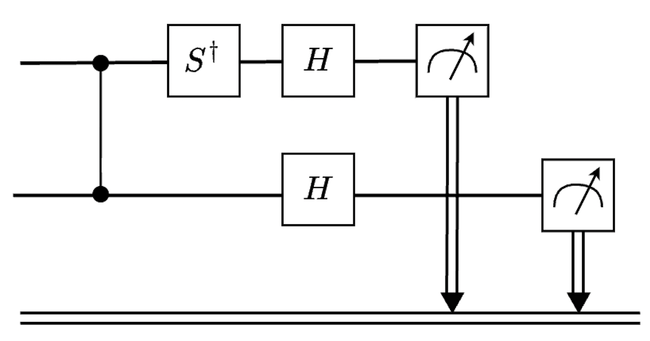
In this example, and we have
Thus, measuring on the first qubit, the second qubit, and both the first and second qubit correspond to results for ,, and . The worst case of transformation circuit requires gates [39].
III Converting Quantum input to Quantum output
For quantum input, we prepare eigenstates of each Pauli basis at the beginning of a circuit. Initializing states for all bases requires a total of states for quantum input qubits. Taking one cut as an example, the states to be prepared include , , , , , and . The initialization requirement can be reduced to preparing only , , , and states by substituting the identity operation with and , though initial states are still required [31].
Drawing inspiration from quantum process tomography [42, 18], applying a random Pauli string at the front of the circuit is analogous to entangling each qubit with an ancilla qubit in a Bell state and then applying a measurement on that Pauli basis. We provide a formula and example Fig. 4 below.
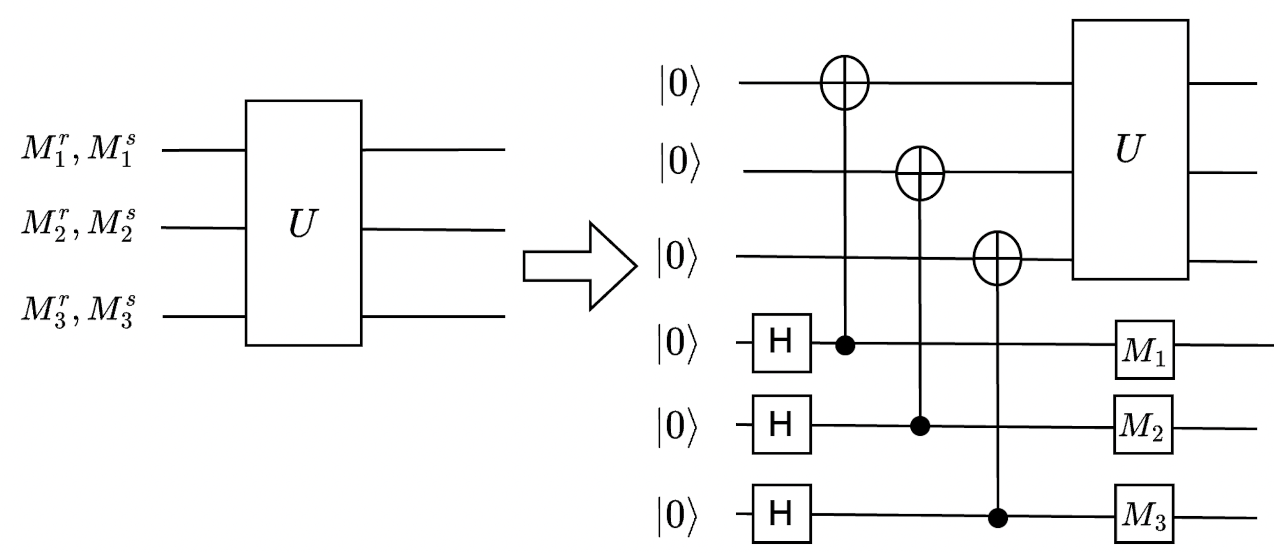
Assuming we have an -qubit circuit . All qubits are quantum input qubits, which means ( is used only in this section). We need to initialize different eigenstate and on -th qubit, where and are eigenstates of , and . Just like ancilla-assisted quantum process tomography, we can rewrite via entangling each qubit with an ancilla-qubit in a bell state and then measure ancilla-qubit on basis, as shown below:
| (9) |
where and is bell state on -th qubit and -th qubit. Following the qubit ordering, may be . This strategy simplifies the implementation as the one circuit can be used for all initialization schemes.
IV Efficient Circuit Wire Cutting based on commuting groups
Currently, CutQC [31] represents the most promising work in circuit cutting. It encompasses the most widely used decomposition method for circuit cutting. Thus, in this paper, we compare our circuit cutting technique with CutQC.
In CutQC, each density matrix at a cutting location need to be decomposed into four Pauli operators. When multiple cuts are introduced, the number of decomposed Pauli operators scales exponentially. Drawing inspiration from [33], we can apply the MUBs-based grouping on Pauli operators as discussed in Section II-B. This approach allows for partitioning the set , consisting of Pauli operators, into commuting groups, each group contains Pauli operators. By utilizing this method, information can be obtained more efficiently.
We provide a more detailed derivation as follows. More specifically, recall from Eq. 6 that the subcircuit of -th fragment with operator can be expressed as:
| (10) |
Then, we convert quantum input to quantum output by adding ancilla qubits as discussed in Sec. III. This yields
where the state is given by
, and is the Bell state entangling the -th qubit and the -th qubit. For convenient we denote the quantum input qubit index set after conversion as .
We can then apply MUBs-based grouping on Pauli operators and perform simultaneous measurement on qubits within each group. Denote as one of commuting groups. Denote as a transformation circuit (Sec. II-B) corresponding . We have
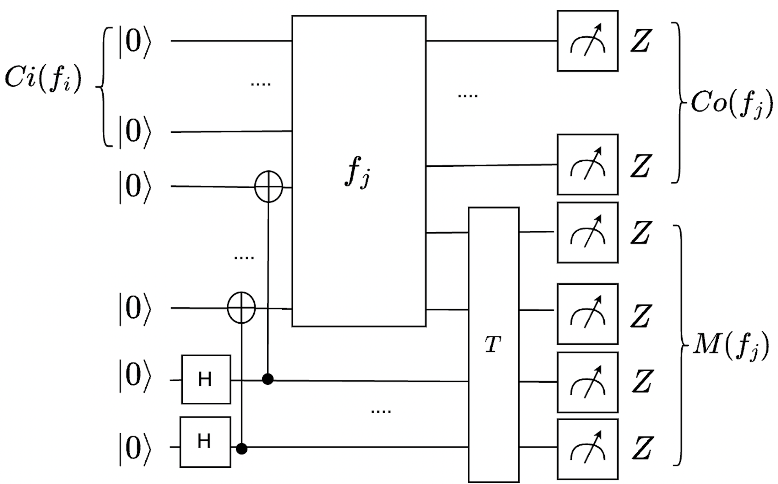
where . Now, we can measure on the basis to get results for the commuting group. Any subcircuit state can be obtained through post-processing of , if . A sample example is shown in Fig. 5.
After simultaneously measuring on all commuting groups for each fragment and completing all fragments, we reconstruct the result of the uncut circuit using the Eq.7.
This method maximally leverage the advantage of MUBs-based grouping. There is a straightforward benefit that the number of circuits to run decreases from to . However, we can see this method is not optimal for all kinds of fragments considering the shot budget. We will provide more analysis in the next section.
V Shot Analysis and Trade-offs
V-A Shot Analysis
Let be the number of shots required to estimate an observable from an -qubit circuit. According to CutQC, the total number of shots required for the -th fragment should be
| (13) |
The exponential factors is the number of subcircuits (initialization-measurement pair) to run. We first replace quantum inputs with quantum outputs, which changes the total number of shots to
| (14) |
Then, exploiting MUBs-based grouping further reduces the total number of circuits to execute polynomially, yielding the sampling complexity:
| (15) |
We can perform a more detailed analysis with explicit form of . Typically, it is reasonable to set that
| (16) |
as there are possible states from at the quantum output qubit need to be fully measure. Thus, we can reform our method results as:
| (17) |
Compared to Eq. 13, our method polynomially better than CutQC when and performs slightly worse when there are no quantum outputs. Thus, we give an Algorithm 1 that applies the CutQC method when there are no quantum outputs, and utilizes our efficient circuit cutting technique when there is quantum outputs. The algorithm can guarantee that all fragments achieve shot savings.
V-B Trade-offs Regarding Circuit Width and Depth
As discussed in Sec. II-B, to perform simultaneous measurement, we need to apply a transformation circuit to the measurement qubits. The maximum size of this transformation circuit is , where represents the squaure of the total number of quantum input and output qubits. For smaller fragments, this process may not be well-suited to current noisy devices, as it introduces ancilla qubits, additional CNOT gates, and a transformation circuit. The number of gates in a fragment should be to ensure that the impact of the transformation circuit is negligible. Additionally, introducing more ancilla qubits lead to an increase in circuit width.
VI Experiment
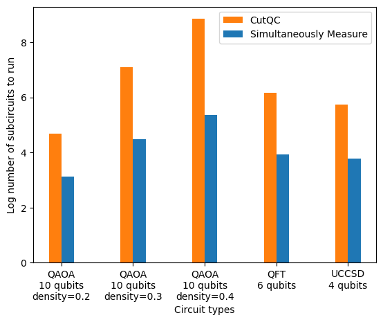
We first demonstrate that our method significantly reduces the number of subcircuits required for execution. As shown in Fig. 7, we observe the number of subcircuits necessary for various circuits. We utilize the Mixed-Integer Programming (MIP) model from CutQC [31] to determine cutting locations. The maximum subcircuit width is set to , where is number of qubit in the uncut circuit. We explore fragment numbers ranging from 1 to 10, selecting the configuration that yields the minimum number of subcircuits. The circuits under investigation include quantum approximate optimization algorithms (QAOA) with randomly generated graphs of different densities, as well as quantum Fourier transform (QFT) and Unitary Coupled-Cluster Single and Double excitations variational form (UCCSD )[43].
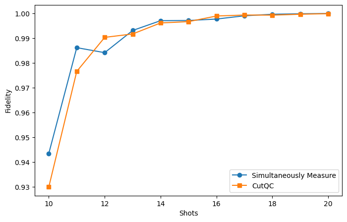
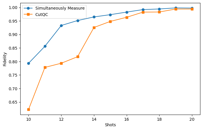
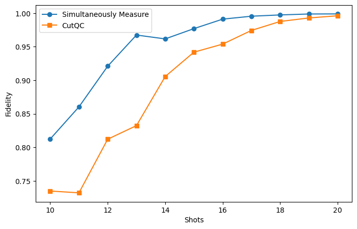
To assess the overhead in terms of shots, we employ randomly generated circuits as benchmarks. We sampled several circuits randomly as fragments and combined them to create our test uncut circuits. The tests were carried out with 2, 3, and 4 cuts. All circuits were executed on the Aer Simulator without introducing any hardware noise.
VII Conclusion
In this paper, we introduce a new method for executing circuit cutting that reduces the shot overhead associated with quantum measurements. Our method first converts all quantum inputs into outputs using ancilla-assisted initialization. We then use a transformation circuit composed the quantum inputs and outputs to enable simultaneous measurement within a commuting group. Our analysis focuses on determining under which conditions MUBs-based grouping yields improvements, and we give an algorithm to guarantee shot savings. We conclude by demonstrating that our method outperforms previous techniques on saving shots and reducing number of quantum circuits to run.
References
- [1] A. Bayerstadler, G. Becquin, J. Binder, T. Botter, H. Ehm, T. Ehmer, M. Erdmann, N. Gaus, P. Harbach, M. Hess et al., “Industry quantum computing applications,” EPJ Quantum Technology, vol. 8, no. 1, p. 25, 2021.
- [2] F. Bova, A. Goldfarb, and R. G. Melko, “Commercial applications of quantum computing,” EPJ quantum technology, vol. 8, no. 1, p. 2, 2021.
- [3] J. Gambetta, “Ibm’s roadmap for scaling quantum technology,” IBM Research Blog (September 2020), 2020.
- [4] R. LaRose, A. Mari, S. Kaiser, P. J. Karalekas, A. A. Alves, P. Czarnik, M. El Mandouh, M. H. Gordon, Y. Hindy, A. Robertson, P. Thakre, M. Wahl, D. Samuel, R. Mistri, M. Tremblay, N. Gardner, N. T. Stemen, N. Shammah, and W. J. Zeng, “Mitiq: A software package for error mitigation on noisy quantum computers,” Quantum, vol. 6, p. 774, Aug. 2022. [Online]. Available: https://doi.org/10.22331/q-2022-08-11-774
- [5] M. H. Abobeih, Y. Wang, J. Randall, S. J. H. Loenen, C. E. Bradley, M. Markham, D. J. Twitchen, B. M. Terhal, and T. H. Taminiau, “Fault-tolerant operation of a logical qubit in a diamond quantum processor,” Nature, vol. 606, no. 7916, p. 884–889, May 2022. [Online]. Available: http://dx.doi.org/10.1038/s41586-022-04819-6
- [6] A. A. Saki, A. Katabarwa, S. Resch, and G. Umbrarescu, “Hypothesis testing for error mitigation: How to evaluate error mitigation,” 2023.
- [7] J. Gambetta, “Quantum-centric supercomputing: The next wave of computing,” Dec 2022. [Online]. Available: https://research.ibm.com/blog/next-wave-quantum-centric-supercomputing
- [8] T. Ayral, F.-M. Le Régent, Z. Saleem, Y. Alexeev, and M. Suchara, “Quantum divide and compute: Hardware demonstrations and noisy simulations,” in 2020 IEEE Computer Society Annual Symposium on VLSI (ISVLSI). IEEE, 2020, pp. 138–140. [Online]. Available: https://ieeexplore.ieee.org/document/9155024
- [9] T. Ayral, F.-M. L. Régent, Z. Saleem, Y. Alexeev, and M. Suchara, “Quantum divide and compute: exploring the effect of different noise sources,” SN Computer Science, vol. 2, no. 3, pp. 1–14, 2021. [Online]. Available: https://doi.org/10.1007/s42979-021-00508-9
- [10] J. Liu, A. Gonzales, and Z. H. Saleem, “Classical simulators as quantum error mitigators via circuit cutting,” arXiv preprint arXiv:2212.07335, 2022. [Online]. Available: https://arxiv.org/abs/2212.07335
- [11] Z. H. Saleem, T. Tomesh, M. A. Perlin, P. Gokhale, and M. Suchara, “Quantum Divide and Conquer for Combinatorial Optimization and Distributed Computing,” arXiv preprint, Jul. 2021. [Online]. Available: https://arxiv.org/abs/2107.07532
- [12] A. Lowe, M. Medvidović, A. Hayes, L. J. O’Riordan, T. R. Bromley, J. M. Arrazola, and N. Killoran, “Fast quantum circuit cutting with randomized measurements,” 2022. [Online]. Available: https://arxiv.org/abs/2207.14734
- [13] D. T. Chen, Z. H. Saleem, and M. A. Perlin, “Quantum divide and conquer for classical shadows,” arXiv preprint arXiv:2212.00761, 2022. [Online]. Available: https://arxiv.org/abs/2212.00761
- [14] D. Chen, B. Baheri, V. Chaudhary, Q. Guan, N. Xie, and S. Xu, “Approximate quantum circuit reconstruction,” in 2022 IEEE International Conference on Quantum Computing and Engineering (QCE). IEEE, 2022, pp. 509–515.
- [15] D. T. Chen, E. H. Hansen, X. Li, V. Kulkarni, V. Chaudhary, B. Ren, Q. Guan, S. Kuppannagari, J. Liu, and S. Xu, “Efficient quantum circuit cutting by neglecting basis elements,” arXiv preprint arXiv:2304.04093, 2023.
- [16] D. T. Chen, E. H. Hansen, X. Li, A. Orenstein, V. Kulkarni, V. Chaudhary, Q. Guan, J. Liu, Y. Zhang, and S. Xu, “Online detection of golden circuit cutting points,” in 2023 IEEE International Conference on Quantum Computing and Engineering (QCE), vol. 1. IEEE, 2023, pp. 26–31.
- [17] G. Uchehara, T. M. Aamodt, and O. Di Matteo, “Rotation-inspired circuit cut optimization,” arXiv preprint arXiv:2211.07358, 2022. [Online]. Available: https://arxiv.org/abs/2211.07358
- [18] J. B. Altepeter, D. Branning, E. Jeffrey, T. Wei, P. G. Kwiat, R. T. Thew, J. L. O’Brien, M. A. Nielsen, and A. G. White, “Ancilla-assisted quantum process tomography,” Physical Review Letters, vol. 90, no. 19, p. 193601, 2003.
- [19] F. De Martini, A. Mazzei, M. Ricci, and G. M. D’Ariano, “Exploiting quantum parallelism of entanglement for a complete experimental quantum characterization of a single-qubit device,” Physical Review A, vol. 67, no. 6, p. 062307, 2003.
- [20] W. K. Wootters, “Quantum mechanics without probability amplitudes,” Foundations of physics, vol. 16, no. 4, pp. 391–405, 1986.
- [21] J. Schwinger, “Unitary operator bases,” Proceedings of the National Academy of Sciences, vol. 46, no. 4, pp. 570–579, 1960.
- [22] I. Ivonovic, “Geometrical description of quantal state determination,” Journal of Physics A: Mathematical and General, vol. 14, no. 12, p. 3241, 1981.
- [23] W. K. Wootters and B. D. Fields, “Optimal state-determination by mutually unbiased measurements,” Annals of Physics, vol. 191, no. 2, pp. 363–381, 1989.
- [24] J. Lawrence, Č. Brukner, and A. Zeilinger, “Mutually unbiased binary observable sets on qubits,” Physical Review A, vol. 65, no. 3, p. 032320, 2002.
- [25] K. Mitarai and K. Fujii, “Constructing a virtual two-qubit gate by sampling single-qubit operations,” New Journal of Physics, vol. 23, no. 2, p. 023021, 2021.
- [26] C. Ufrecht, M. Periyasamy, S. Rietsch, D. D. Scherer, A. Plinge, and C. Mutschler, “Cutting multi-control quantum gates with zx calculus,” Quantum, vol. 7, p. 1147, 2023.
- [27] H. Harada, K. Wada, and N. Yamamoto, “Doubly optimal parallel wire cutting without ancilla qubits, 2023,” arXiv preprint arXiv:2303.07340.
- [28] L. Brenner, C. Piveteau, and D. Sutter, “Optimal wire cutting with classical communication,” arXiv preprint arXiv:2302.03366, 2023.
- [29] A. Lowe, M. Medvidović, A. Hayes, L. J. O’Riordan, T. R. Bromley, J. M. Arrazola, and N. Killoran, “Fast quantum circuit cutting with randomized measurements,” Quantum, vol. 7, p. 934, 2023.
- [30] T. Peng, A. W. Harrow, M. Ozols, and X. Wu, “Simulating large quantum circuits on a small quantum computer,” Physical review letters, vol. 125, no. 15, p. 150504, 2020.
- [31] W. Tang, T. Tomesh, M. Suchara, J. Larson, and M. Martonosi, “Cutqc: using small quantum computers for large quantum circuit evaluations,” in Proceedings of the 26th ACM International conference on architectural support for programming languages and operating systems, 2021, pp. 473–486.
- [32] M. A. Perlin, Z. H. Saleem, M. Suchara, and J. C. Osborn, “Quantum circuit cutting with maximum-likelihood tomography,” npj Quantum Information, vol. 7, no. 1, p. 64, 2021. [Online]. Available: https://doi.org/10.1038/s41534-021-00390-6
- [33] P. Gokhale, O. Angiuli, Y. Ding, K. Gui, T. Tomesh, M. Suchara, M. Martonosi, and F. T. Chong, “Minimizing state preparations in variational quantum eigensolver by partitioning into commuting families,” arXiv preprint arXiv:1907.13623, 2019.
- [34] R. Cleve, A. Ekert, C. Macchiavello, and M. Mosca, “Quantum algorithms revisited,” Proceedings of the Royal Society of London. Series A: Mathematical, Physical and Engineering Sciences, vol. 454, no. 1969, pp. 339–354, 1998.
- [35] Y. Wang and W. Cui, “classical shadow tomography with mutually unbiased bases,” arXiv preprint arXiv:2310.09644, 2023.
- [36] R. Shankar, Principles of Quantum Mechanics. Springer Science & Business Media, 2012.
- [37] R. A. Horn and C. R. Johnson, Matrix Analysis. Cambridge University Press, 2012.
- [38] D. Gottesman, Stabilizer codes and quantum error correction. California Institute of Technology, 1997.
- [39] U. Seyfarth and K. S. Ranade, “Construction of mutually unbiased bases with cyclic symmetry for qubit systems,” Physical Review A, vol. 84, no. 4, p. 042327, 2011.
- [40] B. Reggio, N. Butt, A. Lytle, and P. Draper, “Fast partitioning of pauli strings into commuting families for optimal expectation value measurements of dense operators,” arXiv preprint arXiv:2305.11847, 2023.
- [41] S. Aaronson and D. Gottesman, “Improved simulation of stabilizer circuits,” Physical Review A, vol. 70, no. 5, p. 052328, 2004.
- [42] R. Levy, D. Luo, and B. K. Clark, “Classical shadows for quantum process tomography on near-term quantum computers,” Physical Review Research, vol. 6, no. 1, p. 013029, 2024.
- [43] P. K. Barkoutsos, J. F. Gonthier, I. Sokolov, N. Moll, G. Salis, A. Fuhrer, M. Ganzhorn, D. J. Egger, M. Troyer, A. Mezzacapo et al., “Quantum algorithms for electronic structure calculations: Particle-hole hamiltonian and optimized wave-function expansions,” Physical Review A, vol. 98, no. 2, p. 022322, 2018.