EACO-RAG: Edge-Assisted and Collaborative RAG with
Adaptive Knowledge Update

Abstract.

Large Language Models are revolutionizing Web, mobile, and Web of Things systems, driving intelligent and scalable solutions. However, as Retrieval-Augmented Generation (RAG) systems expand, they encounter significant challenges related to scalability, including increased delay and communication overhead. To address these issues, we propose EACO-RAG, an edge-assisted distributed RAG system that leverages adaptive knowledge updates and inter-node collaboration. By distributing vector datasets across edge nodes and optimizing retrieval processes, EACO-RAG significantly reduces delay and resource consumption while enhancing response accuracy. The system employs a multi-armed bandit framework with safe online Bayesian methods to balance performance and cost. Extensive experimental evaluation demonstrates that EACO-RAG outperforms traditional centralized RAG systems in both response time and resource efficiency. EACO-RAG effectively reduces delay and resource expenditure to levels comparable to, or even lower than, those of local RAG systems, while significantly improving accuracy. This study presents the first systematic exploration of edge-assisted distributed RAG architectures, providing a scalable and cost-effective solution for large-scale distributed environments.

1. Introduction

Large Language Models (LLMs) are reshaping Web, mobile, and Web of Things (WoT) systems by enabling more intelligent, adaptive, and scalable solutions. Their integration enhances user experience with accurate, real-time, and context-aware responses, improving system efficiency and unlocking new capabilities for autonomous processing (wu2022autoformalization, ), recommendations (lyu2023llm, ; ren2024representation, ), and decision-making (yang2023large, ; li2022pre, ).

Retrieval-Augmented Generation (RAG) extends LLMs’ capabilities by integrating retrieval mechanisms that provide relevant context from a knowledge base, further improving the accuracy of generated responses. Its expanding presence in healthcare, education, and legal services is driving rapid adoption, with the market projected to grow at a compound annual growth rate of 44.7% between 2024 and 2030 (Grandview2024, ).

As RAG services continue to expand rapidly, scalability challenges can result in Quality of Service (QoS) degradation, with typical concerns including reduced answer quality (chen2024benchmarking, ) and increased response delay (hofstatter2023fid, ; yu2024evaluation, ). Commonly, RAG systems convert text into vector representations stored in databases and are hosted alongside language models in centralized data centers. However, as service demand grows, these centralized architectures encounter problems such as increased delay, communication overhead with end users, and inefficient global database searches. A notable trend is the deployment of LLMs at the edge (zhang2024edgeshard, ; qu2024mobile, ), which shows promising potential to reduce generation delay. In light of this, we argue that shifting RAG services toward edge-assisted distributed architectures could be a highly effective approach to address these scalability and performance challenges.

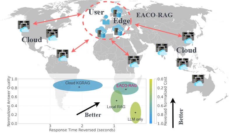
Figure 1. Overview of Edge-assisted and Collaborative RAG (EACO-RAG), together with a comparison to other solutions, showing its improvements in answer quality, response time, and cost efficiency.

More specifically, edge integration could help by strategically planning retrieval and generation based on end-user behavioral patterns in proximity, reducing delay, and improving performance. Edge nodes can analyze behaviors locally to preemptively optimize retrievals. In a cascaded fashion, simpler tasks may be processed at the edge, while complex queries are escalated to central databases in the cloud. This approach can not only reduce communication overhead and enhance system efficiency, but also allow edge nodes to dynamically update their knowledge bases, enhancing their localized query handling capabilities and further reducing communications with central cloud servers.

Despite these benefits, integrating edge computing with RAG systems presents challenges. For example, user queries span a wide range of topics, requiring a knowledge base that potentially encompasses global information. Maintaining such vast data locally at edge nodes is impractical due to storage and resource constraints. Further, in distributed environments, optimizing retrieval processes to minimize resource consumption while ensuring real-time performance can be complicated, where such factors as physical distance to data centers, data volume, and node load all can influence retrieval delays.

Traditional distributed databases and search engines have addressed data scalability but often exhibit static architectures lacking flexibility, making it difficult to adapt to dynamic user needs in the RAG context. Additionally, centralized query processing increases delay and communication overhead, while the absence of intelligent, dynamic updates limits efficient responses to changing demands. These limitations further complicate the balance between efficient data retrieval and adaptive performance in edge environments.

In this paper, we explore the following research question: ”Can RAG systems be optimized to minimize resource consumption while maintaining performance through adaptive knowledge updates and collaboration at edge nodes?” Addressing this question provides insights into designing scalable, efficient, and intelligent RAG systems capable of meeting complex and dynamic user needs.

We provide a positive answer by introducing EACO-RAG, a distributed RAG system that fully integrates edge assistance through adaptive knowledge updates and collaboration at the edge. EACO-RAG distributes vector datasets across multiple edge nodes, optimizing the retrieval process by dynamically updating local knowledge bases. By leveraging edge computing and inter-node collaboration, the system addresses key challenges such as scalability, delay reduction, and resource efficiency in large-scale distributed environments. In this context, optimizing the RAG system involves the critical challenge of minimizing costs while meeting strict accuracy and delay constraints.

To tackle this, we model the optimization problem as a multi-armed bandit, utilizing safe online Bayesian methods to manage the trade-off between accuracy, delay, and cost. As shown in Figure 1, EACO-RAG effectively reduces both delay and resource expenditure to levels comparable to, or even lower than, those of local RAG systems, while significantly improving accuracy. In our experiments, EACO-RAG achieves a 76.7% reduction in cost and a 74.2% reduction in delay compared to KGRAG-3B, with only an 11.5% sacrifice in accuracy. Our contributions are the following:

• To our best knowledge, we are the first efforts to systematically propose and investigate an edge-assisted distributed RAG architecture, EACO-RAG, which uses adaptive knowledge updates and collaborations at edge nodes to minimize delay and communication overhead, offering a cost-efficient solution for large-scale distributed environments.

• We propose adaptive knowledge update mechanisms that enable edge nodes to dynamically adjust their local knowledge bases, adapting to user behavior and evolving demands in real-time.

• We design optimized retrieval processes that are capable to integrate edge collaborations to better balance real-time performance with resource efficiency, ensuring scalability across distributed systems.

• We conduct extensive experiments evaluating EACO-RAG, which demonstrate the superiority of our EACO-RAG solution in response times and resource utilization compared to traditional centralized RAG systems.

2. Motivation

In this section, we first perform a series of trace-driven analyses to identify the bottlenecks, strengths, and limitations of existing RAG systems, which motivate us to propose our EACO-RAG solution.

2.1. Tradeoffs in RAG Systems

Table 1. LLM Information.

ID	Model Name	Model Size	Deploy
1	qwen2.5:0.5b	398MB	Mobile Edge
2	qwen2.5:1.5b	986MB	Mobile Edge
3	qwen2.5:3b	1.9GB	Mobile Edge
4	qwen2.5:7b	4.7GB	Edge Server
5	qwen2.5:14b	9GB	Edge Server
6	qwen2.5:32b	20GB	Cloud Server
7	qwen2.5:72b	47GB	Cloud Server

A typical RAG system consists of two main components: the generator (i.e., LLM) and the knowledge database. In our analysis, we focus on the bottlenecks of a generalized RAG system, specifically in terms of accuracy, delay and computational resource consumption, as determined by these two components. The models presented in Table 1 represent a selection of LLM configurations chosen for this paper. Note that here we highlight the importance of deploying LLM-based RAG systems at the edge (qin2024robust, ), evaluating them in terms of cost, accuracy, and delay.

Generator: For the generator, increasing the number of parameters typically enhances accuracy but at the cost of longer generation times and higher computational requirements. To evaluate these trade-offs, we conducted experiments with 500 question-answer (QA) pairs using an NVIDIA RTX 4090, which represents a typical edge configuration, reflecting the computational power commonly available at the edge (lim2024accelerating, ). The results, presented in Figures LABEL:Figures/MEASUREMENT/Figure1_models_flops_size.pdf and LABEL:Figures/MEASUREMENT/Figure1_models_accuracy_generatetime.pdf, show how model size impacts accuracy, generation time, and resource consumption, where the accuracy was measured by comparing the generated responses with correct answers using GPT-4o (langchain2023autoevaluator, ).

Some key trends can be observed from the figure: accuracy improves significantly as models scale from small to medium (0.5B–7B parameters) and from medium to large (7B–32B parameters). However, these accuracy gains come with substantial trade-offs. For instance, while generation times remain under 1 second for models up to 14B parameters, they surpass 4 seconds for the 32B model due to the limitations of the RTX 4090. Moreover, deploying models larger than 7B on mobile devices is impractical due to their high computational demands. The 32B model, in particular, exceeds the capacity of typical edge servers. As shown in Figure LABEL:Figures/MEASUREMENT/Figure1_models_flops_size.pdf, the average TFLOP consumption per query increases dramatically beyond the 7B parameter threshold.

These computational constraints suggest that larger models are often better suited for cloud deployment, but this introduces additional network delays. Figure LABEL:Figures/MEASUREMENT/Figure2_distance_delay.pdf depicts the network delay measured via ICMP protocol over varying distances (with ”City A” representing the local region, and other locations anonymized). The delay rises from under 10ms in local regions to over 100ms, and occasionally over 200ms, for more distant regions. While cloud-based models benefit from faster generation times due to superior computational resources, their overall service time is predominantly affected by network delays, especially across longer distances. This underscores the challenge of balancing model accuracy with real-time performance.

Given the delay and cost issues associated with cloud-based large models, deploying LLMs at the edge becomes critical. However, edge deployment presents accuracy challenges, making the use of an integrated knowledge database in RAG systems essential for improving performance.

Knowledge Base In RAG systems, two key parameters for optimizing performance are chunk size and the number of retrieved documents per query (Top K). These parameters directly influence retrieval efficiency and the quality of the generated responses. Chunk size defines how the knowledge base is segmented (measured in token count), while Top K determines the number of documents (or chunks) retrieved per query (edge2024local, ). Figure LABEL:Figures/MEASUREMENT/Figure3.1_chunksize.pdf explores the relationship between chunk size and accuracy. While larger chunk sizes can reduce redundancy and speed up retrieval, they may also lower accuracy by increasing the likelihood of irrelevant information being included in the LLM’s context. Figure LABEL:Figures/MEASUREMENT/Figure3.2_TopK.pdf examines the trade-off between the number of retrieved chunks (Top K) and system performance. Increasing Top K enhances the LLM’s contextual knowledge but also leads to higher delay, computational costs and generating hallucinations from excessive context. Through comparative analysis, we determined that a chunk size of 300 tokens and a Top K of 20 achieve an optimal balance between retrieval efficiency and answer accuracy for edge-deployed LLM-based RAG systems.

2.2. Advantages and Disadvantages of Current RAG Systems

After identifying the bottlenecks in current RAG systems, we now examine their strengths and weaknesses in context-dependent scenarios. To do this, we collected 500 QA from a public dataset about the Harry Potter series. These questions were categorized into 20 clusters based on their semantic correlations. We evaluated three systems: an LLM-only, a local RAG, and a cloud Knowledge Graph-based RAG (KGRAG). Figure LABEL:Figures/MEASUREMENT/Figure4_accuracy.pdf shows the accuracy of these systems across the different classes. It can be seen that over 50% of the questions were context-dependent, meaning that when domain-specific knowledge was required, the accuracy of standalone LLMs dropped to nearly zero (e.g., in clusters such as 5, 9 and 17). While RAG systems partially mitigate this issue, improving accuracy by 15% to 20% over LLMs, they are still constrained by the scope of their local knowledge bases. If relevant information is missing, the benefit of RAG is minimal. In contrast, KGRAG systems, which use structured knowledge graphs, showed a significant increase in accuracy—an average improvement over 40% compared to LLMs—when the required information was available in the knowledge base.

However, these gains do not come for free. Although KGRAG dramatically enhances accuracy, it also notably increases generation time. As shown in Figure LABEL:Figures/MEASUREMENT/Figure4_generation_time.pdf, while generation times for LLM and basic RAG systems remain relatively stable across various classes, the generation times for KGRAG fluctuate due to the overhead of retrieving from huge knowledge bases. Depending on the retrieval complexity, generation times can spike from the usual 0.5 seconds to over 7 seconds (as seen in clusters 10, 11, 13, 16 and 19). On average, KGRAG’s collaborative retrieval process extends generation time by an additional 1.95 seconds compared to standalone LLMs.

These results highlight both the strengths and limitations of traditional RAG systems, reinforcing the need for more efficient designs. While RAG systems improve accuracy by integrating domain-specific knowledge, their overall effectiveness is hampered by issues like fluctuating generation times and limited knowledge base coverage. This observation inspired us to explore a more adaptive approach. By dynamically updating the knowledge base based on user queries and leveraging the vast number of distributed edge devices, we can harness the power of each edge node’s local database. Through collaboration between these distributed edge resources, queries can be addressed more effectively at the edge, improving contextual understanding while maintaining reasonable generation times. This approach is particularly valuable for context-dependent applications. In the next section, we will delve into the design of our distributed edge RAG system with adaptive knowledge update.

3. EACO-RAG Overview and System Design

High-performance models, such as O1 models, present significant challenges for service providers due to their heavy computational requirements and extended generation times, both of which negatively affect the overall quality of service (QoS). Furthermore, these models often underperform when handling context-dependent queries, which are common in industrial applications. Resolving such queries typically necessitates additional model fine-tuning or the use of retrieval-augmented generation (RAG), further complicating the operational workflow.

To address these challenges, in EACO-RAG, we propose an online adaptive knowledge update system that optimizes response quality, generation time, and costs by adaptively selecting from LLMs, RAG, and knowledge-graph RAG (KGRAG) based on contextual information. Moreover, in this system, simpler queries are processed by edge nodes located near the user, while more complex queries are escalated to the cloud for handling, operating in a cascading structure to efficiently manage resource allocation.

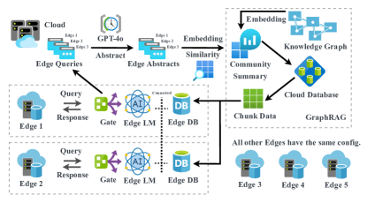
Figure 6. Workflow of the EACO-RAG system design.

As depicted in Figure 6, user queries are initially stored in the cloud as they pass through the gate in edge nodes, with this data being used to update the local databases at the edge. Once a sufficient number of queries are collected, the system generates an abstract using an LLM (e.g., GPT-4o), producing summaries such as “Names and functions of spells in the wizarding world” or “Rules, history, and key events in Quidditch”, which reflect common topics queried by nearby users. These abstracts are then compared to community summaries stored in the knowledge graph by embedding both sets of data and assessing their similarity. The most relevant data chunks are identified and downloaded to the edge for local RAG operations. If the abstract changes based on recent user queries at the edge, the local database is updated accordingly.

On the other hand, when a new query is received at the edge, the system determines the optimal retrieval and generation strategy based on query complexity, network delay, and similarity to other edge databases. However, query complexity and similarity to other edge databases are not straightforward to obtain. Specifically, query complexity can be assessed using a simple classifier (jeong2024adaptive, ), while similarity to other edge databases is determined by comparing the embedding of the user query with the summaries from each edge. This approach facilitates efficient retrieval from relevant edge nodes and enhances overall system stability.

Furthermore, the gate mechanism plays a vital role in reducing generation time and operational costs while preserving service quality. It determines the necessity of retrieval and selects the most efficient approach—whether local, edge, cloud retrieval or bypassing retrieval for simpler queries. Additionally, the gate decides whether to generate responses using a local model or delegate to the more powerful cloud models. The local knowledge base is continuously updated, and the gate dynamically optimizes the RAG retrieval and generation path, minimizing costs while ensuring that response accuracy and generation delay meet the required thresholds.

As a provider of LLM-based services, our primary objectives are to ensure response quality, reduce generation delay, and minimize operational costs. To address this, we model the problem as a contextual multi-armed bandit and employ a gate architecture based on Safe Online Bayesian Optimization. This approach minimizes total costs while maintaining the necessary accuracy and delay standards, effectively balancing the use of both edge and cloud resources. Detailed implementation strategies are presented in the subsequent sections.

4. Cost Modelling and Optimization

4.1. Cost Modelling with Contextual Multi-Armed Bandit

Our objective is to minimize the total operational costs incurred by the service provider, which include both resource usage and delay costs. Resource costs arise from computational expenses related to model generation and knowledge base retrieval, while delay costs reflect the opportunity cost of increased response times due to network latency and model generation delays. The system must satisfy two key constraints: (i) answer accuracy must exceed a defined threshold $\rho_{\min}$, and (ii) response time must remain below a real-time limit $h_{\max}$.

Context: At each time $t$, the context is represented as $c^{t}:=[d^{t}_{\text{cloud}},d^{t}_{\text{edge}},s^{t},q^{t}]\in\mathcal{C}$, where $d^{t}_{\text{cloud}}$ and $d^{t}_{\text{edge}}$ represent network delays to the cloud and edge servers, respectively, $s^{t}$ indicates the similarity between the query and the summaries in the edge database, and $q^{t}$ reflects the complexity of the query. The context space is denoted by $\mathcal{C}$.

Control Policies: Let $d^{t}:=[r^{t},g^{t}]\in\mathcal{D}$ represent the control policy at time $t$, where $r^{t}$ denotes the retrieval location and $g^{t}$ specifies the generation location. Retrieval $r^{t}$ can occur locally, at the edge, from the cloud or non-retrieval, while generation $g^{t}$ can take place at either the edge or cloud. These policies are dynamically adjusted based on the real-time context to optimize cost.

The system carefully balances service provider costs, delay, and accuracy. Local and edge-based databases provide low-cost, low-delay responses that are well-suited for simple, highly relevant queries, which can be efficiently processed at the local level. For more complex queries that demand broader knowledge or greater accuracy, the system retrieves data from the cloud-based knowledge graph. While this incurs higher costs and greater delay, it delivers more accurate and comprehensive responses. Similarly, for response generation, the system balances between the faster but less powerful edge models, which suffice for basic queries, and the more accurate cloud models, which, though more costly, ensure the precision needed for more complex queries.

The total cost function is defined as:

(1) $$u^{t}(c^{t},d^{t})=\delta_{1}\cdot u_{\text{r}}^{t}(c^{t},d^{t})+\delta_{2}\cdot u_{\text{d}}^{t}(c^{t},d^{t}),$$

where $\delta_{1}$ and $\delta_{2}$ are weights for resource and delay costs, respectively. $u_{\text{r}}^{t}(c^{t},d^{t})$ represents the computational cost incurred by the service provider during model generation and data retrieval, while $u_{\text{d}}^{t}(c^{t},d^{t})$ accounts for delay time costs, including those related to network network and model generation delays, as excessive delays can reduce system efficiency and increase operational overhead for the provider.

The optimization problem is formulated as:

(2) $$\min_{\{d^{t}\}_{t=1}^{T}}\sum_{t=1}^{T}u^{t}(c^{t},d^{t})$$

$$\text{s.t.}\quad\rho^{t}(c^{t},d^{t})\geq\rho_{\min},\quad\forall t\leq T,$$

$$\quad\quad h^{t}(c^{t},d^{t})\leq h_{\max},\quad\forall t\leq T,$$

where $\rho^{t}(c^{t},d^{t})$ is the accuracy of the generated answer, and $h^{t}(c^{t},d^{t})$ represents the model response time at time $t$.

This formulation focuses on minimizing the service provider’s operational costs while ensuring that both accuracy and delay constraints are met. The system adapts dynamically to evolving network conditions and database content using online learning techniques to continuously refine decision-making strategies. As network delay or database content changes, the system adjusts retrieval and generation strategies in real time to maintain optimal performance while minimizing costs. In the next section, we will explore the use of Safe Online Bayesian Optimization to develop algorithms that ensure these constraints are respected, while minimizing service provider costs and maintaining high quality of service.

4.2. Safe Online Bayesian Optimization

In this part, we present our solution to the contextual multi-armed bandit problem discussed earlier to further enhance the system’s decision-making process in dynamic environments. To this end, we introduce a Bayesian online optimization approach, summarized in Algorithm 1, which utilizes Gaussian Processes (GPs) to capture the nonlinearities and correlations within the system, while also quantifying the uncertainty in function estimation. This algorithm enables the system to dynamically balance exploration and exploitation, leading to performance improvements over time with minimal cost and delay. Further details on the algorithm, including its implementation and operation, are provided in the following section.

Function Approximator. We use Gaussian Processes (GPs) to estimate the cost and constraint functions, modeling them as collections of random variables with joint Gaussian distributions (williams2006gaussian, ; duvenaud2014automatic, ). Let $x\in\mathcal{X}=\mathcal{C}\times\mathcal{D}$ represent a context-decision pair. Each unknown function is modeled as a sample from $\text{GP}(\mu(x),k(x,x^{\prime}))$, where $\mu(x)$ is the mean function and $k(x,x^{\prime})$ is the kernel function (duvenaud2014automatic, ) that captures the covariance between points $x$ and $x^{\prime}$. We assume a prior distribution where $\mu(x)=0$ and $k(x,x^{\prime})<1$, meaning the distribution is unconditioned by data.

Given this prior and a set of observed data, we compute the posterior distribution of the functions in closed form. Let $X_{T}=\{x_{1},\dots,x_{T}\}$ represent the observed context-decision pairs up to time $T$. The observations for cost, accuracy, and response time are denoted as $y_{T}^{(0)}=\{u_{1},\dots,u_{T}\}$, $y_{T}^{(1)}=\{\rho_{1},\dots,\rho_{T}\}$, and $y_{T}^{(2)}=\{h_{1},\dots,h_{T}\}$, respectively, assuming independent Gaussian noise with variance $\sigma^{2}$. The posterior distribution remains Gaussian, with updated mean $\mu_{T}^{(i)}(x)$ and covariance $k_{T}^{(i)}(x,x^{\prime})$ for each function $i$ (cost, accuracy, response time) given by:

(3) $$\mu_{T}^{(i)}(x) =k_{T}^{(i)}(x)^{T}(K_{T}^{(i)}+\sigma^{2}I_{T})^{-1}y_{T}^{(i)}$$

(4) $$k_{T}^{(i)}(x,x^{\prime}) =k^{(i)}(x,x^{\prime})-k_{T}^{(i)}(x)^{T}(K_{T}^{(i)}+\sigma^{2}I_{T})^{-1}k_{T}^{(i)}(x^{\prime}),$$

where $k_{T}^{(i)}(x)=[k^{(i)}(x_{1},x),\dots,k^{(i)}(x_{T},x)]^{T}$ is the covariance vector between $x$ and the observed points in $X_{T}$, $K_{T}^{(i)}$ is the kernel matrix $[k^{(i)}(x,x^{\prime})]_{x,x^{\prime}\in X_{T}}$, and $I_{T}$ is the identity matrix of size $T$. The index $i$ corresponds to different objective functions: $i=0$ for cost, $i=1$ for accuracy, and $i=2$ for response time.

For any unobserved $x\in\mathcal{X}$, the posterior mean and covariance for function $i$ are derived from the prior, observed data $X_{T}$, and corresponding observations $y_{T}^{(i)}$ using the equations above.

Safe Set. Identifying the safe set, consisting of control policies that meet system constraints in a given context, is essential for maintaining performance within acceptable limits. The safe set depends on both the control policies and the context. For instance, in our problem, a context change such as a complex query or high network delay may require shifting from local resources to cloud-based resources, increasing response time. As a result, policies that perform well under low-delay conditions might not satisfy the response time constraint in high-delay scenarios.

We define the safe set $S_{t}$ at time $t$ as the set of context-decision pairs that satisfy all system constraints:

(5) $$S_{t}=\{x\in\mathcal{X}\mid\mu_{t}^{(1)}(c_{t},x)-\beta\sigma_{t}^{(1)}(c_{t},x)\geq\rho_{\min}$$

$$\quad\land\mu_{t}^{(2)}(c_{t},x)+\beta\sigma_{t}^{(2)}(c_{t},x)\leq h_{\max}\}$$

Where $\mu_{t}^{(i)}(c_{t},x)$ and $\sigma_{t}^{(i)}(c_{t},x)$ represent the mean and uncertainty (standard deviation) of the Gaussian Process predictions for function $i$ (accuracy or response time) at time $t$. The exploration parameter $\beta$ balances exploration and exploitation, while $\rho_{\min}$ and $h_{\max}$ denote the minimum accuracy and maximum response time, respectively.

Determining the safe set is challenging due to the noisy nature of system performance indicators, such as accuracy and response time, which are affected by the stochastic environment. To address this, we use Gaussian Processes (GPs) to estimate the safe set based on observed data. At each time step $t$, after observing the context $c_{t}$ and decision $x_{t}$, the GP models are updated, refining the estimates of the mean $\mu_{t}^{(i)}(c_{t},x)$ and uncertainty $\sigma_{t}^{(i)}(c_{t},x)$ for both cost and constraint functions. Because of the correlations between nearby points in the context-decision space, updating the posterior for one point influences the estimates for surrounding points, which affects the composition of the safe set in the following time step, $t+1$. This dynamic update process allows the system to continually adjust its estimation of the safe set, ensuring that it adapts to changing contexts while maintaining performance within the required constraints.

1 Inputs: Control space $\mathcal{X}$, Safe seed set $S_{0}$, kernel $k$, $\rho_{\min}$ (minimum accuracy), $h_{\max}$ (maximum response time), exploration parameter $\beta$, cost weights $\delta_{1}$, $\delta_{2}$

2Initialization: $Z_{0}=\emptyset,y_{0}^{(0)}=\emptyset,y_{0}^{(1)}=\emptyset,y_{0}^{(2)}=\emptyset$;

3

4for $t=1,\dots,T_{0}$ (Exploration phase) do

5       Observe context $c_{t}$;

6       Randomly select $x_{t}$ from $\mathcal{X}$ (random exploration);

7      

8      Observe $h_{t}(c_{t},x_{t})$ (response time), $\rho_{t}(c_{t},x_{t})$ (accuracy), $u_{\text{r}}^{t}(c_{t},x_{t})$ (resource cost), $u_{\text{d}}^{t}(c_{t},x_{t})$ (delay cost);

9      

10      Compute total cost:  $u^{t}(c_{t},x_{t})=\delta_{1}\cdot u_{\text{r}}^{t}(c_{t},x_{t})+\delta_{2}\cdot u_{\text{d}}^{t}(c_{t},x_{t})$;

11      

12      Update $Z_{t}=Z_{t-1}\cup\{c_{t},x_{t}\}$;

13       Update GP posteriors:

14        $y_{t}^{(0)}\leftarrow y_{t-1}^{(0)}\cup u^{t}(c_{t},x_{t})$ (update cost posterior);

15        $y_{t}^{(1)}\leftarrow y_{t-1}^{(1)}\cup\rho_{t}(c_{t},x_{t})$ (update accuracy posterior);

16        $y_{t}^{(2)}\leftarrow y_{t-1}^{(2)}\cup h_{t}(c_{t},x_{t})$ (update response time posterior);

17      

18 end for

19

20for $t=T_{0}+1,\dots,T$ (Exploitation phase) do

21       Observe context $c_{t}$;

22       Compute $\mu_{t-1}^{(i)}(c_{t},x)$ and $\sigma_{t-1}^{(i)}(c_{t},x)$ for all $i=0,1,2$, using the posterior from the previous iteration;

23      

24      Estimate the safe set:

25        $S_{t}=S_{0}\cup\{x\in\mathcal{X}\mid\mu_{t}^{(1)}(c_{t},x)-\beta\sigma_{t}^{(1)}(c_{t},x)\geq\rho_{\min}$

26        $\land\mu_{t}^{(2)}(c_{t},x)+\beta\sigma_{t}^{(2)}(c_{t},x)\leq h_{\max}\}$;

27      

28      Select $x_{t}=\arg\min_{x\in S_{t}}\mu_{t}^{(0)}(c_{t},x)-\sqrt{\beta_{t}}\sigma_{t}^{(0)}(c_{t},x)$ (acquisition function);

29      

30      Observe $h_{t}(c_{t},x_{t})$ (response time), $\rho_{t}(c_{t},x_{t})$ (accuracy), $u_{\text{r}}^{t}(c_{t},x_{t})$ (resource cost), $u_{\text{d}}^{t}(c_{t},x_{t})$ (delay cost);

31      

32      Compute total cost:  $u^{t}(c_{t},x_{t})=\delta_{1}\cdot u_{\text{r}}^{t}(c_{t},x_{t})+\delta_{2}\cdot u_{\text{d}}^{t}(c_{t},x_{t})$;

33      

34      Update $Z_{t}=Z_{t-1}\cup\{c_{t},x_{t}\}$;

35       Update GP posteriors:

36        $y_{t}^{(0)}\leftarrow y_{t-1}^{(0)}\cup u^{t}(c_{t},x_{t})$ (update cost posterior);

37        $y_{t}^{(1)}\leftarrow y_{t-1}^{(1)}\cup\rho_{t}(c_{t},x_{t})$ (update accuracy posterior);

38        $y_{t}^{(2)}\leftarrow y_{t-1}^{(2)}\cup h_{t}(c_{t},x_{t})$ (update response time posterior);

39      

40 end for

Algorithm 1 AdaptiveEdge SafeOBO Algorithm

Step One: Exploration. The first phase of the AdaptiveEdge SafeOBO algorithm serves as a warm-up step, focusing on exploring the control space $\mathcal{X}$ without initially considering the safe set. The purpose of this warm-up phase is to gather foundational data on the cost, accuracy, and response time functions by randomly selecting context-decision pairs from $\mathcal{X}$. At each time step $t$, a context $c_{t}$ is observed, and the algorithm randomly selects a decision $x_{t}$ from the control space. This exploration allows the algorithm to collect sufficient observations of system performance under varying conditions, creating a solid basis for more informed decision-making in later steps. Formally, the decision $x_{t}$ is chosen as:

(6) $$x_{t}=\text{Randomly select from }\mathcal{X}.$$

Once a decision is made, the corresponding accuracy $\rho_{t}(c_{t},x_{t})$, response time $h_{t}(c_{t},x_{t})$, and total cost $u^{t}(c_{t},x_{t})$ are observed. These observations are used to update the Gaussian Process (GP) posteriors for the cost, accuracy, and response time functions, setting the foundation for the exploitation phase.

Step Two: Exploitation and Safe Set Optimization. In the second phase, the algorithm transitions from random exploration to strategic decision-making, utilizing the data gathered in the exploration phase. At this point, AdaptiveEdge SafeOBO estimates a safe set $S_{t}$ of context-decision pairs that meet the system’s constraints on accuracy and response time. Specifically, the safe set includes decisions expected to satisfy both the minimum accuracy $\rho_{\min}$ and the maximum response time $h_{\max}$, with confidence bounds based on the GP posteriors:

(7) $$S_{t}=S_{0}\cup\{x\in\mathcal{X}\mid\mu_{t}^{(1)}(c_{t},x)-\beta\sigma_{t}^{(1)}(c_{t},x)\geq\rho_{\min}$$

$$\quad\land\mu_{t}^{(2)}(c_{t},x)+\beta\sigma_{t}^{(2)}(c_{t},x)\leq h_{\max}\}$$

Within the safe set, the algorithm selects the decision $x_{t}$ that minimizes the expected total cost while considering the uncertainty (exploration) in the GP model. This is done by optimizing the following acquisition function:

(8) $$x_{t}=\arg\min_{x\in S_{t}}\mu_{t}^{(0)}(c_{t},x)-\sqrt{\beta_{t}}\sigma_{t}^{(0)}(c_{t},x),$$

where $\mu_{t}^{(0)}(c_{t},x)$ and $\sigma_{t}^{(0)}(c_{t},x)$ are the posterior mean and variance of the cost function at time $t$, and $\beta_{t}$ controls the trade-off between exploration and exploitation.

By iteratively updating the safe set and selecting decisions within it, the algorithm ensures optimal performance while respecting accuracy and response time constraints. As more observations are gathered, the GP models are refined, allowing the system to continuously improve decision-making, optimizing both safety and utility over time.

5. Implementation and Evaluation

5.1. Prototype Implementation

Our prototype implementation of the EACO-RAG system adopts a dual-tier architecture that balances efficiency and performance by deploying models at both the edge and in the cloud. The system utilizes two distinct models, each tailored for different query types based on complexity and resource requirements:

• Edge 3B Model: A compact language model deployed on edge nodes, optimized for straightforward or moderately complex queries. This model delivers low-delay responses with minimal computational overhead, making it ideal for scenarios where speed and resource efficiency are essential.

• Cloud 72B Model: A high-capacity language model deployed in the cloud, dedicated to handling more complex and cross-domain queries. Although it incurs higher computational costs and longer delay, this model ensures highly accurate responses for tasks requiring deep knowledge or contextual understanding.

The architecture dynamically selects between these models based on query complexity, processing simple requests at the edge to reduce delay, while directing more demanding queries to the cloud. This flexible design optimizes response times and resource allocation across distributed environments.

In our experimental setup, the edge nodes are powered by NVIDIA RTX 4090 GPUs, enabling rapid inference and scalability at the local level. The cloud-based 72B model serves as a benchmark for high-accuracy, complex query processing, although it incurs higher delays, highlighting the trade-off between edge efficiency and cloud-level precision.

By effectively distributing tasks between edge and cloud resources, the EACO-RAG system demonstrates significant improvements in both query response times and resource utilization, underscoring the potential of EACO-RAG for practical applications.

Figure 7. Converge evaluation with different exploration rounds.

5.2. Convergence

To evaluate the convergence of the EACO-RAG system, we consider and measure a series of parameters, including different exploration rounds $T_{0}$, varying delay cost weights $\delta_{2}$, and the impact on overall cost under specific accuracy and delay thresholds.

To specifically assess the convergence speed and the impact of $T_{0}$ on the balance between exploration and exploitation, we first plot the cost against the number of iterations for $T_{0}=5,10,20,50,100$. In Figure 7, the cost variation across increasing iterations for different $T_{0}$ values is illustrated. The results indicate that as $T_{0}$ increases, the system’s convergence rate initially accelerates but then slows down. This suggests that, in our scenario, approximately 10 exploration rounds are sufficient for gathering the necessary initial information, whereas excessive warm-up rounds may impede convergence. Notably, regardless of the $T_{0}$ value, the system eventually converges to a similar cost level, demonstrating the robustness of the EACO-RAG algorithm.

Table 2. TFLOP consumption per second of waiting for various server-side NVIDIA GPUs.

GPU Model	FP64 (Double Precision)
NVIDIA GeForce RTX 4090	1.29 TFLOPS
NVIDIA Tesla P100	4.70 TFLOPS
NVIDIA Tesla V100	7.80 TFLOPS
NVIDIA A100 Tensor Core	9.70 TFLOPS
NVIDIA H100 Tensor Core	60.00 TFLOPS

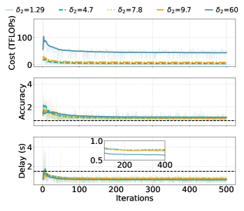
Figure 8. Convergence evaluation under varying delay cost weights. The weights are based on the TFLOP per second generated by different GPU models. The cost is represented as total TFLOPs.

Figure 8 presents the system’s performance under different delay cost weights $\delta_{2}$, including total cost (measured in TFLOPs), accuracy, and delay (in seconds). We set the resource cost weight $\delta_{1}$ to 1, as resource cost is directly measured in TFLOPs. Delay cost weights $\delta_{2}$ are chosen based on the typical TFLOP performance of server GPUs in double-precision (FP64) computations, as detailed in Table LABEL:table:gpu. After convergence, we observe that as $\delta_{2}$ increases, the total cost rises, but delay decreases due to its increased weighting in the cost function. In practice, an optimal balance between cost, accuracy, and delay must be determined based on the specific application requirements.

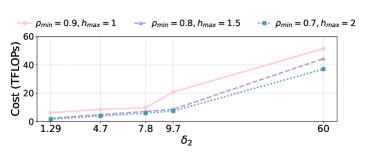
Figure 9. Cost variation as a function of $\delta_{2}$ under different accuracy and delay thresholds.

Figure 9 shows how cost varies with $\delta_{2}$ under different accuracy and delay thresholds. In addition to the general trend of increasing cost with higher $\delta_{2}$ values, we note a faster rise in cost when stricter accuracy and delay thresholds are applied. The relationship between cost and $\delta_{2}$ is nonlinear, and the jump points are influenced by the thresholds, suggesting that certain GPUs may be more suitable for minimizing cost under specific thresholds.

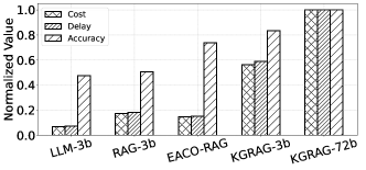
Figure 10. Comparison of LLM, RAG, KGRAG, and our proposed EACO-RAG method, evaluated based on normalized cost, delay, and accuracy.

5.3. Performance Comparison

In Figure 10, we compare the performance of LLM (LLM-3b), local RAG (RAG-3b), cloud KGRAG (KGRAG-3b and KGRAG-70b), and our proposed EACO-RAG method across three key metrics: cost, delay, and accuracy. The values in the figure are normalized to enable a consistent comparison across these different metrics.

Cost and Delay: LLM-3B exhibits the lowest cost and delay, as it does not require additional retrieval operations. EACO-RAG’s cost and delay are slightly higher than LLM-3B, but significantly lower than other RAG methods, demonstrating its cost-effectiveness and delay advantages. Compared to KGRAG-3B, EACO-RAG achieves a 76.7% reduction in cost and a 74.2% reduction in delay, while only sacrificing 11.5% in accuracy. KGRAG-72B, on the other hand, has the highest cost and delay due to its use of a large model and complex knowledge graph retrieval process.

Accuracy: LLM-3B has the lowest accuracy, reflecting the limitations of relying solely on a smaller model to handle complex queries. EACO-RAG’s accuracy is significantly higher than both LLM-3B and RAG-3B, approaching the performance of KGRAG-3B. Compared to RAG-3B, EACO-RAG achieves a 51% improvement in accuracy with comparable cost and delay, indicating that its adaptive knowledge updating mechanism effectively enhances the quality of responses.

In summary, EACO-RAG reduces cost and delay through its edge-assisted and collaborate design while improving accuracy by leveraging its adaptive knowledge update mechanism.

6. Related Work

Retrieval-Augmented Generation Enhancements. Retrieval-Augmented Generation (RAG) improves language models (LMs) by integrating relevant text from knowledge bases (lewis2020retrieval, ). Extensions like Adaptive RAG (jeong2024adaptive, ), Corrective RAG (yan2024corrective, ), and Self-RAG (asai2023self, ) address retrieval strategy limitations and query complexity. These methods adjust retrieval based on query difficulty to enhance performance. Mallen et al. (mallen-etal-2023-trust, ) classify query complexity using entity frequency, applying binary decisions on retrieval sufficiency. Qi et al. (qi-etal-2021-answering, ) use fixed operations (retrieval, reading, reranking), requiring specialized LM training. Self-RAG (asai2023self, ) retrieves, critiques, and generates dynamically, though uniform query handling remains suboptimal. RAG systems are also being integrated with 6G edge networks (huang2024toward, ). Traditional methods like Adaptive-RAG and Corrective-RAG refine retrieval based on query complexity but often rely on centralized frameworks. EACO-RAG, by contrast, uses edge computing to distribute knowledge across multiple nodes, reducing delays and communication overhead while dynamically updating local databases.

Cost-Effective Large Language Model Usage. Reducing LLM deployment costs is an active research focus. Techniques like model quantization (xiao2023smoothquant, ; park2023lut, ) and pruning (ma2024llm, ) cut costs but may reduce performance and require specialized hardware. LLM distillation, where smaller models mimic larger ones, offers a solution. Caching LLM responses for routine queries (stogiannidis2023cache, ; zhu2023optimalcaching, ; gill2024privacy, ; li2024scalm, ) or reusing key-value states during inference (liu2024cachegen, ; yao2024cacheblend, ) are other strategies. FrugalGPT (chen2023frugalgpt, ) uses prompt engineering and model multiplexing to select model size based on query complexity, while model multiplexing dynamically chooses the appropriate model size (bang2023gptcache, ; kim2023biglittle, ). Techniques like model quantization and LLM distillation reduce computational costs but require specialized hardware. EACO-RAG offers a holistic solution, combining edge and cloud resources to optimize retrieval and generation, minimizing resource use and operational costs through a multi-armed bandit framework.

Resource Allocation Strategies in Edge Computing. Optimizing resource allocation in edge computing focuses on balancing delay, energy, and processing power (wang2018joint, ). Techniques like task offloading and resource scheduling aim to minimize latency and energy consumption (naouri2021novel, ). Edge-cloud collaboration dynamically allocates resources between edge nodes and cloud servers (gu2023ai, ). Recent advancements in AI and reinforcement learning improve adaptability and scalability in heterogeneous edge environments, yielding significant efficiency and cost gains (xiong2020resource, ). Conventional edge computing focuses on task offloading within local environments. EACO-RAG introduces inter-node collaboration, allowing dynamic knowledge sharing and optimizing resource allocation across a network of distributed edge devices.

7. Conclusion

This paper introduced EACO-RAG, an edge-assisted collaborative RAG system designed to reduce network delay and resource consumption in large-scale deployments while maintaining accuracy. By leveraging edge computing for adaptive knowledge updates based on user behavior, EACO-RAG optimizes performance using a contextual multi-armed bandit framework and Safe Online Bayesian Optimization, balancing exploration and exploitation to achieve optimal results efficiently. Experimental results show that EACO-RAG outperforms traditional RAG systems in both response quality and resource efficiency, making it a scalable solution for real-time applications. Future work will focus on enhancing knowledge base management and exploring further optimization techniques.

References

- (1) Y. Wu, A. Q. Jiang, W. Li, M. Rabe, C. Staats, M. Jamnik, and C. Szegedy, “Autoformalization with large language models,” Advances in Neural Information Processing Systems, vol. 35, pp. 32 353–32 368, 2022.
- (2) H. Lyu, S. Jiang, H. Zeng, Y. Xia, Q. Wang, S. Zhang, R. Chen, C. Leung, J. Tang, and J. Luo, “Llm-rec: Personalized recommendation via prompting large language models,” arXiv preprint arXiv:2307.15780, 2023.
- (3) X. Ren, W. Wei, L. Xia, L. Su, S. Cheng, J. Wang, D. Yin, and C. Huang, “Representation learning with large language models for recommendation,” in Proceedings of the ACM on Web Conference 2024, 2024, pp. 3464–3475.
- (4) R. Yang, T. F. Tan, W. Lu, A. J. Thirunavukarasu, D. S. W. Ting, and N. Liu, “Large language models in health care: Development, applications, and challenges,” Health Care Science, vol. 2, no. 4, pp. 255–263, 2023.
- (5) S. Li, X. Puig, C. Paxton, Y. Du, C. Wang, L. Fan, T. Chen, D.-A. Huang, E. Akyürek, A. Anandkumar et al., “Pre-trained language models for interactive decision-making,” Advances in Neural Information Processing Systems, vol. 35, pp. 31 199–31 212, 2022.
- (6) Grand View Research. (2024) Retrieval augmented generation market size, share & trends analysis report. Accessed: 2024-10-11. [Online]. Available: https://www.grandviewresearch.com/industry-analysis/retrieval-augmented-generation-rag-market-report
- (7) J. Chen, H. Lin, X. Han, and L. Sun, “Benchmarking large language models in retrieval-augmented generation,” in Proceedings of the AAAI Conference on Artificial Intelligence, vol. 38, no. 16, 2024, pp. 17 754–17 762.
- (8) S. Hofstätter, J. Chen, K. Raman, and H. Zamani, “Fid-light: Efficient and effective retrieval-augmented text generation,” in Proceedings of the 46th International ACM SIGIR Conference on Research and Development in Information Retrieval, 2023, pp. 1437–1447.
- (9) H. Yu, A. Gan, K. Zhang, S. Tong, Q. Liu, and Z. Liu, “Evaluation of retrieval-augmented generation: A survey,” arXiv preprint arXiv:2405.07437, 2024.
- (10) M. Zhang, J. Cao, X. Shen, and Z. Cui, “Edgeshard: Efficient llm inference via collaborative edge computing,” arXiv preprint arXiv:2405.14371, 2024.
- (11) G. Qu, Q. Chen, W. Wei, Z. Lin, X. Chen, and K. Huang, “Mobile edge intelligence for large language models: A contemporary survey,” arXiv preprint arXiv:2407.18921, 2024.
- (12) R. Qin, Z. Yan, D. Zeng, Z. Jia, D. Liu, J. Liu, Z. Zheng, N. Cao, K. Ni, J. Xiong et al., “Robust implementation of retrieval-augmented generation on edge-based computing-in-memory architectures,” arXiv preprint arXiv:2405.04700, 2024.
- (13) H. Lim, J. Ye, S. Abdu Jyothi, and D. Han, “Accelerating model training in multi-cluster environments with consumer-grade gpus,” in Proceedings of the ACM SIGCOMM 2024 Conference, 2024, pp. 707–720.
- (14) Langchain-AI, “Auto evaluator: An evaluation toolkit for language models,” https://github.com/langchain-ai/auto-evaluator, 2023.
- (15) D. Edge, H. Trinh, N. Cheng, J. Bradley, A. Chao, A. Mody, S. Truitt, and J. Larson, “From local to global: A graph rag approach to query-focused summarization,” arXiv preprint arXiv:2404.16130, 2024.
- (16) S. Jeong, J. Baek, S. Cho, S. J. Hwang, and J. C. Park, “Adaptive-rag: Learning to adapt retrieval-augmented large language models through question complexity,” arXiv preprint arXiv:2403.14403, 2024.
- (17) C. K. Williams and C. E. Rasmussen, Gaussian processes for machine learning. MIT press Cambridge, MA, 2006.
- (18) D. Duvenaud, “Automatic model construction with gaussian processes,” Ph.D. dissertation, Apollo - University of Cambridge Repository, 2014.
- (19) P. Lewis, E. Perez, A. Piktus, F. Petroni, V. Karpukhin, N. Goyal, H. Küttler, M. Lewis, W.-t. Yih, T. Rocktäschel et al., “Retrieval-augmented generation for knowledge-intensive nlp tasks,” Advances in Neural Information Processing Systems, 2020.
- (20) S.-Q. Yan, J.-C. Gu, Y. Zhu, and Z.-H. Ling, “Corrective retrieval augmented generation,” arXiv preprint arXiv:2401.15884, 2024.
- (21) A. Asai, Z. Wu, Y. Wang, A. Sil, and H. Hajishirzi, “Self-rag: Learning to retrieve, generate, and critique through self-reflection,” arXiv preprint arXiv:2310.11511, 2023.
- (22) A. Mallen, A. Asai, V. Zhong, R. Das, D. Khashabi, and H. Hajishirzi, “When not to trust language models: Investigating effectiveness of parametric and non-parametric memories,” in Proceedings of the 61st Annual Meeting of the Association for Computational Linguistics (Volume 1: Long Papers), A. Rogers, J. Boyd-Graber, and N. Okazaki, Eds. Toronto, Canada: Association for Computational Linguistics, Jul. 2023, pp. 9802–9822. [Online]. Available: https://aclanthology.org/2023.acl-long.546
- (23) P. Qi, H. Lee, T. Sido, and C. Manning, “Answering open-domain questions of varying reasoning steps from text,” in Proceedings of the 2021 Conference on Empirical Methods in Natural Language Processing, M.-F. Moens, X. Huang, L. Specia, and S. W.-t. Yih, Eds. Online and Punta Cana, Dominican Republic: Association for Computational Linguistics, Nov. 2021, pp. 3599–3614. [Online]. Available: https://aclanthology.org/2021.emnlp-main.292
- (24) X. Huang, Y. Tang, J. Li, N. Zhang, and X. S. Shen, “Toward effective retrieval augmented generative services in 6g networks,” IEEE Network, 2024.
- (25) G. Xiao, J. Lin, M. Seznec, H. Wu, J. Demouth, and S. Han, “Smoothquant: Accurate and efficient post-training quantization for large language models,” in International Conference on Machine Learning. PMLR, 2023, pp. 38 087–38 099.
- (26) G. Park, M. Kim, S. Lee, J. Kim, B. Kwon, S. J. Kwon, B. Kim, Y. Lee, D. Lee et al., “Lut-gemm: Quantized matrix multiplication based on luts for efficient inference in large-scale generative language models,” in The Twelfth International Conference on Learning Representations, 2023.
- (27) X. Ma, G. Fang, and X. Wang, “Llm-pruner: On the structural pruning of large language models,” Advances in neural information processing systems, vol. 36, 2024.
- (28) I. Stogiannidis, S. Vassos, P. Malakasiotis, and I. Androutsopoulos, “Cache me if you can: An online cost-aware teacher-student framework to reduce the calls to large language models,” arXiv preprint arXiv:2310.13395, 2023.
- (29) B. Zhu, Y. Sheng, L. Zheng, C. Barrett, M. I. Jordan, and J. Jiao, “On optimal caching and model multiplexing for large model inference,” arXiv preprint arXiv:2306.02003, 2023.
- (30) W. Gill, M. Elidrisi, P. Kalapatapu, A. Anwar, and M. A. Gulzar, “Privacy-aware semantic cache for large language models,” arXiv preprint arXiv:2403.02694, 2024.
- (31) J. Li, C. Xu, F. Wang, I. M. von Riedemann, C. Zhang, and J. Liu, “Scalm: Towards semantic caching for automated chat services with large language models,” arXiv preprint arXiv:2406.00025, 2024.
- (32) Y. Liu, H. Li, Y. Cheng, S. Ray, Y. Huang, Q. Zhang, K. Du, J. Yao, S. Lu, G. Ananthanarayanan et al., “Cachegen: Kv cache compression and streaming for fast large language model serving,” in Proceedings of the ACM SIGCOMM 2024 Conference, 2024, pp. 38–56.
- (33) J. Yao, H. Li, Y. Liu, S. Ray, Y. Cheng, Q. Zhang, K. Du, S. Lu, and J. Jiang, “Cacheblend: Fast large language model serving with cached knowledge fusion,” arXiv preprint arXiv:2405.16444, 2024.
- (34) L. Chen, M. Zaharia, and J. Zou, “Frugalgpt: How to use large language models while reducing cost and improving performance,” arXiv preprint arXiv:2305.05176, 2023.
- (35) F. Bang, “Gptcache: An open-source semantic cache for llm applications enabling faster answers and cost savings,” in Proceedings of the 3rd Workshop for Natural Language Processing Open Source Software (NLP-OSS 2023), 2023.
- (36) S. Kim, K. Mangalam, J. Malik, M. W. Mahoney, A. Gholami, and K. Keutzer, “Big little transformer decoder,” arXiv preprint arXiv:2302.07863, 2023.
- (37) P. Wang, C. Yao, Z. Zheng, G. Sun, and L. Song, “Joint task assignment, transmission, and computing resource allocation in multilayer mobile edge computing systems,” IEEE Internet of Things Journal, vol. 6, no. 2, pp. 2872–2884, 2018.
- (38) A. Naouri, H. Wu, N. A. Nouri, S. Dhelim, and H. Ning, “A novel framework for mobile-edge computing by optimizing task offloading,” IEEE Internet of Things Journal, vol. 8, no. 16, pp. 13 065–13 076, 2021.
- (39) H. Gu, L. Zhao, Z. Han, G. Zheng, and S. Song, “Ai-enhanced cloud-edge-terminal collaborative network: Survey, applications, and future directions,” IEEE Communications Surveys & Tutorials, 2023.
- (40) X. Xiong, K. Zheng, L. Lei, and L. Hou, “Resource allocation based on deep reinforcement learning in iot edge computing,” IEEE Journal on Selected Areas in Communications, vol. 38, no. 6, pp. 1133–1146, 2020.