DeCaf: A Causal Decoupling Framework for OOD Generalization on Node Classification
Abstract
Graph Neural Networks (GNNs) are susceptible to distribution shifts, creating vulnerability and security issues in critical domains. There is a pressing need to enhance the generalizability of GNNs on out-of-distribution (OOD) test data. Existing methods that target learning an invariant (feature, structure)-label mapping often depend on oversimplified assumptions about the data generation process, which do not adequately reflect the actual dynamics of distribution shifts in graphs. In this paper, we introduce a more realistic graph data generation model using Structural Causal Models (SCMs), allowing us to redefine distribution shifts by pinpointing their origins within the generation process. Building on this, we propose a casual decoupling framework, DeCaf, that independently learns unbiased feature-label and structure-label mappings. We provide a detailed theoretical framework that shows how our approach can effectively mitigate the impact of various distribution shifts. We evaluate DeCaf across both real-world and synthetic datasets that demonstrate different patterns of shifts, confirming its efficacy in enhancing the generalizability of GNNs.
1 Introduction
Graph Neural Networks (GNNs) perform node classification tasks by learning the relationships between node features, local structures, and node labels on a training graph. They have demonstrated promising performance across various applications, such as social recommendation, traffic forecasting, and chemical property prediction [1]. However, their success largely relies on the in-distribution (ID) assumption [2]. In real life, test samples are often collected from different distributions such as various geographical areas, domains, or time periods, leading to potentially different and unknown distributions from the training data. Consequently, the model might learn an incorrect mapping of (feature, structure)-label relationships that fail on test data, leading to a well-known out-of-distribution (OOD) problem [3].
One de facto approach to graph OOD generalization [4, 5, 6, 7, 8] assumes that there exist “true” correlations between input and labels that are invariant under distribution shifts. These correlations can be obtained by identifying the non-causal/spurious parts of the input (e.g. sub-ego-networks or subvectors of the node’s embedding). However, they model the features of a node and its neighborhood as a single entity. By doing so, they implicitly assume that the shifts in features () and structures () occur simultaneously and cannot be separated from one another. A detailed discussion on the limitations of existing methods is provided in Appendix 1.1.
However, we claim that such an assumption may fail on many real-world graphs (e.g., citation graphs, social networks). The generation process of graph data is complex: for a node, its features and local topology can be viewed as reflections of its true representations by different “observers”. For example, to predict whether someone might be prone to drug addiction based on their online social networks, we can analyze their profile features (e.g., job, social status, photos) as the public image they choose to present. The accounts they follow can indicate additional aspects (e.g., hobbies, personal life, mental status) not explicitly stated in their profiles. Both the profile features and their network connections provide insights into the user’s true status, but they highlight different facets through distinct mappings. Together, they offer valuable information for predicting the target behavior. However, these elements may display varying distribution patterns over time or across different locations. For instance, individuals might disclose different profile information depending on state laws, or their network connections might change following updates to the social network’s recommendation algorithm. Such variations can occur separately and both impact the original (feature, structure)-label relationships.
We formalize the graph generation process as a Structural Causal Model (SCM). Based on the graph generation process, we redefine the types of distribution shifts. Previously, graph OOD largely followed definitions from general data: for covariate shift, ; for concept shift, [9]. We reformulate the definition, attributing covariate shift to changes in the true representations, and define two types of concept shift based on the different mappings of features and structure, respectively. We justify the universality of our new definitions.
To this end, we demonstrate that any type of distribution shift can alter the (feature, structure)-label mapping. However, we observe that because the generating mechanism of the features or structures does not change, the true feature-label or structure-label mappings should remain invariant. Based on this observation, we propose a causal decoupling framework, DeCaf, that learns unbiased feature-label or structure-label mappings as causal effects for predicting node labels. Intuitively, DeCaf answers the question: “What information about the label can the node features provide when its local structure is unavailable, and vice versa?" We provide a theoretical analysis to demonstrate the feasibility and effectiveness of DeCaf. We also present an implementable paradigm of DeCaf that utilizes Generalized Robinson Decomposition to estimate the causal effects as a practical solution. We evaluate our proposed method across both real-world and synthetic datasets with different patterns of shifts. The results consistently demonstrate that our proposed method improves the generalization ability of GNNs on the node classification task.
2 Casual Decoupling Framework
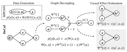
In this section, we introduce the causal decoupling framework, DeCaf, which performs node classification by independently estimating the treatment effects of node features and neighborhood representations. We develop a comprehensive theoretical foundation to support the rationale: Initially, we present a novel graph generation process using a Structural Causal Model (SCM), which contrasts with the assumptions underlying most GNN models (section 2.1). Utilizing this SCM, we redefine various types of distribution shifts in graph data and analyze how each SCM element changes under these shifts (Section 2.2). This analysis leads to the development of the causal decoupling framework, which seeks to separately assess the direct impacts of node features and neighborhood representations on node labels (section 2.3). To achieve an unbiased estimation of their impact, we treat the impact as a treatment effect, which can be estimated with a casual estimation model that considers the confounder effect (section 2.4). We visually summarize this conceptual flow in Figure 1. Following this theoretical basis, we propose a practical end-to-end paradigm that leverages SOTA casual inference technologies to estimate the decoupled representations and make final predictions, as detailed in Section 2.4.
2.1 Graph generation process
We build a SCM for graph generation processes based on the assumption that for each node , there exists an unobserved raw latent vector that is fully informative about its “true nature”, and its ground-truth label, , is an affine transformation of to the label space. For a connected graph , where is the node set and is the edge set, we directly observe node features , and the adjacency matrix . Although the latent variable matrix cannot be directly observed, we believe there exists a “hidden observer” that can observe and decide and based on some rules.
Definition 1.
The “true nature”, denoted as z, is an unobserved latent variable representing “all facts” (extrinsic or intrinsic) about a node in a graph. For a node instance , knowing provides sufficient information about its features and its connectivity with any other node as . Specifically, there exists a function such that and a function such that .
An intuitive example. A person’s “true nature” would encompass not only extrinsic details like gender and education but also intrinsic qualities such as personality and beliefs. These intrinsic features are difficult to measure directly and completely, yet they largely influence a person’s public profile (e.g., personal webpage) and social relationships (e.g., friendships). For example, the content of a personal webpage is shaped not only by true experiences but also by the individual’s personality, which affects how those experiences are presented. Understanding a person’s true nature provides a complete view of their behaviors.
For simplicity of analysis, we assume the features of node , , is an affine transformation of , and is decided by the similarity between some linear transformations of and .
Assumption 1.
The generation process of given can be expressed as follows:
| (1) |
| (2) |
| (3) |
where , , , and are constant linear transformation matrices, and are constant vectors, is euclidean distance, and is a constant number to control the density of the adjacency matrix.
We claim that Assumption 1 can be generalized to different scenarios. For instance, a homophilous graph would have assigned with the same values as ; conversely, a heterophilous graph would have and to be opposite with each other; when or are assigned with values close to zeros, the connection will show more randomized behaviors.
According to Assumption 1, node ’s feature is only dependent on ; however, its connection with other nodes depends on the latent variable of the whole graph, and it seemingly brings spill-over effects/inferences, which occurs when the treatment received by one instance affects the outcome of another instance. This effect breaks Stable Unit Treatment Value Assumption (SUTVA) that the potential outcomes of any unit do not vary with the treatment assigned to other units. It is one of the core assumptions in causal inference as we will discuss in section 2.4. To address this, we investigate the correlation between the features of a central node and its neighboring nodes. As the adjacent matrix does not contain the features of neighboring nodes, we define an embedding matrix
| (4) |
where is the -th vector of which represents the neighborhood information of all nodes, is a linear transformation matrix, and is the node set of -hop neighbors of node . is an aggregation function (e.g. mean). Although this may introduce undesired correlations between samples that complicate our analysis, we show that under the Law of Large Numbers, experiences negligible spillover effects from other samples. Further details are discussed in Appendix 4.
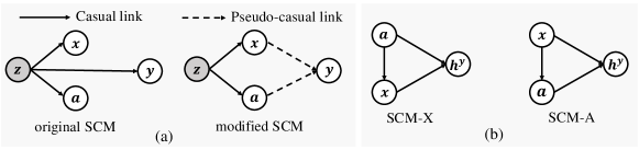
To this end, we build a SCM in Figure 2 (a-left) to represent the relationships between the variables , , , and . When developing a machine learning model, the Close World Assumption is generally followed, that the training data encompasses sufficient information to make accurate predictions. Applying that to our case, given the unobservability of , we need to assume that all features within pertinent to are recoverable through and . For the convenience of our narrative, we assume is directly caused by and , and we replace the causal link between and with pseudo-causal links and . Future analysis is based on the modified SCM in Figure 2 (a-right). Based on the modified SCM, the correlation between and is constituted by two back door paths: and . Similarly, the correlation between and is constituted by , . For the paths and , is the common cause (confounder) of and .
2.2 Types of distribution shifts on graph data
Based on the proposed SCM, we redefine the covariate shift and the concept shift on graph data. Bearing in mind that OOD generalization is impossible without any assumption in the data generalization process, we make a constraint such that the conditional distribution between the latent variable and the ground truth label should remain invariant across different domains (e.g. , or ). We justify it by pointing out that both and characterize the intrinsic nature of the data point, and the invariance of their correlation is necessary to ensure that OOD generalization is possible. Starting with that, we identify different sources of distribution shifts. We attribute covariate shift to the drift of the latent variable .
Definition 2.
(Covariate Shift): while remain the same for training and test data.
We attribute concept shift to the changes in the generation process of node features or the edges with a fixed distribution. We define each case, separately.
Definition 3.
(Concept Shift-X): while and the rest parameters remain the same.
Definition 4.
(Concept Shift-A): while and the rest parameters remain the same.
We investigate and summarize the behavior of the joint distribution of and and the relations between other variables under different distribution shifts in Appendix 5. As it shows, under all three types of distribution shifts, the distribution changes, thus the directly estimated correlation between and with the training set may fail in the test set. On the other hand, at least one of and remains constant under the shifts.
2.3 Graph decoupling
We propose to estimate as the combination of and . However, when predicting with a graph neural network, is often modeled as , where represents the output embedding of the GNN model before the activation, and is the non-linear activation function. Due to the non-linearity of , the assumption that can be estimated as the combination of and can be easily violated. Also, the mapping to the probability space before the combination could potentially lose the rich information delivered by the embedding space. To address this, we perform the combination process in the embedding space instead.
Assumption 2.
The value of can be estimated as the weighted average of the values of individual functions and .
| (5) |
where is a constant hyperparamter that controls the ratio between the contribution of and to the final prediction.
We claim that Assumption 2 is a reasonable assumption when is modeled with message-passing graph neural networks (MPGNNs). Most MPGNNs obtain the representation of the central node by aggregating its neighboring nodes with operations like summing or (weighted) averaging, which can be viewed as a process in which each central/neighboring node shares its “vote” on deciding the outcome. To better make our point, we analyze classification on the Simple Graph Convolution (SGC) model [10]. We show that when a fixed weight is assigned to the central node during the aggregation process, the prediction function of SGC can be written as:
| (6) | ||||
where , is the “normalized” adjacency matrix , , is the degree matrix of , is the number of layers, is the parameterized weights of each layer into a single matrix: . We can view as , and as , which aligns with asssumtion 2. Notice for the adjacency matrix at the first layer does not include self-loops, ensuring that the node feature of the instance itself is not included.
We thus claim that Assumption 2 is reasonable. Note that it only holds when and are unbiased estimations. As shown in Figure 2 (a), and are caused by a common factor , thus they act like confounders of each other through back-door paths and . The direct estimation of and is biased. In the next section, we aim to obtain unbiased estimations of and by considering the confounder effect.
2.4 Casual effect estimation
To clearly understand how changing / directly influences while considering and adjusting for other confounding factors, we propose to treat and as treatment effect of and on the outcome (Section. 2.3). In a generalized causal effect estimation framework where the treatment can be a continuous representation instead of binary values, we can interpret the effect of treatment as “what additional information can provide on predicting the outcome”. In that sense, we want to estimate the treatment effect of and , separately, so each can provide information about the output representation when conditioned on one another. We build two Structural Casual Models to represent the cases where one of / is the treatment and another is the confounder, as shown in Figure 2 (b). Based on the SCMs, we aim to utilize casual effect inference to estimate the following Conditional Average Treatment Effects (CATEs):
| (7) | ||||
| (8) | ||||
where and are counterfactual node features and neighborhood representations. Their definitions will be discussed later. Since the counterfactual outcome is unobservable, we follow the common practice and made the assumptions in Appendix 6 to estimate the CATEs.
We then propose a practical solution to estimate and , and combine them to make predictions. We apply Generalized Robinson Decomposition (GRD) to isolate the causal estimands and reduce the biases when estimating CATEs.
Generalized Robinson Decomposition. GRD is proposed as a generalized version of Robinson Decomposition [11] to adapt graph-structured treatment. Specifically, GRD assumes that the causal effect is a product effect:
Assumption 3.
(Product Effect) We consider the following partial parameterization of :
| (9) |
where , are the representation of the treatment and the confounder; , and , for all .
Assumption 3 has been proven to be mild and can approximate any arbitrary bounded continuous functions with a small error bound [12]. We define propensity features as and . Following the same steps as in Robinson Decomposition, the GRD of Equation 9 is: . Given nuisance estimates and , and can be derived with the optimization problem:
| (10) | ||||
With estimated and , the CATE of treatment variable and its counterfactual given the confounder can be simplified as:
| (11) |
To optimize Equation 10, we can use Structured Intervention Networks (SIN) [12], a two-stage training algorithm to learn and as neural networks and estimate the CATE with Equation 11. In our case, we need to estimate separate set decomposition functions, and , for each casual model, and to apply SIN directly would bring the following drawbacks: 1) By separately applying SIN to our two casual models, it would fail to share the representations of the common factors (e.g. the confounder of one model is the treatment of another); the lack of knowledge sharing could make the learning process less efficient and the learned model prone to overfitting. 2) Unlikely common scenarios where counterfactual treatments are well-defined, in our case, and can not be easily decided. Since they are both continuous values that can span the space, how to define their values in the situation where the node is not treated by the treatment (node features/neighborhood representations)? To address these two problems, we propose Dual Casual Decomposition and Background Counterfactual Selection as components of our method.
2.4.1 Dual casual decomposition
We aim to learn two sets of for SCM-X and SCM-A. We denote them as and , separately. Each casual model is also associated with a set of , denoted as and . Observing that directly applying SIN separately could double the training time and be inefficient, we notice that for our two SCMs, the treatment of one model is the confounder of the other. Leveraging this fact, we allow the embedding of the same entity to be shared across the two models. We propose a new paradigm, named Dual Causal Decomposition, which first learns the common embedding of the two models and then applies a lighter dual version of SIN to estimate the remaining embedding. Our approach effectively reduces model parameters. The complete process is provided in Appendix 8.
2.4.2 Background counterfactual selection
We view the treatment effect as useful information provided by the treatment variables for decision-making in predictions. At each of the casual models, the factual treatment ( or ) received by an instance reveals information about its label. In the counterfactual “untreated” case, the treatment representation should reveal no such information. It is problematic to simply set the counterfactual representation as zeros since an all-zeros embedding does not necessarily mean the absence of information. Instead, for each instance, at each time, we randomly sample a treatment representation from the whole dataset, and we answer the question: what net effect does the factual treatment bring compared to the random counterfactual treatment? We repeat the above process multiple times and average the net effects as the estimated treatment effect.
Specifically, for SCM-A, we randomly sample neighborhood representations with indexes from the datasets as the counterfactual treatment. The counterfactual outcome is then estimated as follows:
| (12) |
Similarly, for SCM-X, the counterfactual outcome is estimated as:
| (13) |
3 Experiments
To evaluate the effectiveness of DeCaf, we aim to answer the following research questions (RQs): RQ1: How well can DeCaf handle covariate shift? RQ2: How well can DeCaf handle concept shift? RQ3: How does the confounder effect between node feature and the neighborhood representation impact the performance of different models, and how well can DeCaf handle this confounder effect?
3.1 Comparison methods
We compare DeCaf with SOTA Graph OOD generalization methods that are applicable to the node classification including IRM [3], REX [5], EERM [13], CIT [14], FLOOD [2], and StableGL [15]. We also compare with empirical risk minimization (ERM) as a baseline. Among these methods, REX [5] requires access to multiple training environments, thus it is only applicable to the OGB-elliptic and Facebook-100 datasets with multiple training graphs. SR-GNN [16] requires access to the input distribution of the test set when training the model and does not apply to the inductive setting studied in this paper. All experiments are conducted on an NVIDIA GeForce RTX 3090 GPU with 24GB memory. We compare DeCaf with the baseline methods regarding their restrictions and complexity in Appendix 9.
| Dataset | Method | SGC | GCN | GAT |
|---|---|---|---|---|
| Cora | ERM | 65.614.28 | 67.940.89 | 66.952.81 |
| IRM | 65.523.01 | 66.042.33 | 65.464.08 | |
| EERM | 65.272.22 | 67.242.86 | 69.502.66 | |
| CIT | 60.511.48 | 61.300.72 | 67.802.28 | |
| FLOOD | 63.584.86 | 62.265.54 | 66.355.43 | |
| StableGL | 59.9613.18 | 65.425.20 | 67.281.11 | |
| DeCaf | 71.411.19 | 70.121.29 | 70.580.49 | |
| Citeseer | ERM | 49.053.15 | 49.581.47 | 52.900.58 |
| IRM | 52.981.86 | 51.821.59 | 51.751.00 | |
| EERM | 44.530.92 | 43.562.10 | 52.634.78 | |
| CIT | 44.215.75 | 49.360.64 | 55.941.94 | |
| FLOOD | 46.754.78 | 49.565.49 | 53.080.51 | |
| StableGL | 51.357.34 | 49.623.29 | 51.501.12 | |
| DeCaf | 59.771.15 | 58.850.51 | 56.711.96 | |
| Amazon | ERM | 86.671.11 | 87.140.33 | 87.710.95 |
| IRM | 86.960.14 | 88.010.40 | 86.791.05 | |
| EERM | 87.630.50 | 88.120.16 | 86.681.43 | |
| CIT | 87.830.92 | 87.460.91 | 82.284.51 | |
| FLOOD | 87.080.73 | 87.330.68 | 85.203.72 | |
| StableGL | 87.260.73 | 87.480.45 | 85.262.82 | |
| DeCaf | 89.670.39 | 88.930.73 | 88.740.57 | |
| Coauthor | ERM | 86.600.91 | 87.660.24 | 80.481.21 |
| IRM | 87.960.52 | 88.750.58 | 78.871.20 | |
| EERM | 84.681.28 | 85.271.04 | OOM | |
| CIT | 84.480.40 | 86.171.52 | 85.600.84 | |
| FLOOD | 83.631.13 | 85.271.04 | OOM | |
| StableGL | 84.480.40 | 86.171.52 | 85.930.76 | |
| DeCaf | 89.200.37 | 88.970.26 | 85.281.42 |
3.2 Performance on covariate shift (RQ1)
We use seven single-graph real-world datasets in which Cora, Citeseer, Amazon-photo and Coauthor-CS are homophilous graphs; Squirrel, Roman-empire and Tolokers are heterophilous graphs. Further details of the above datasets are provided in Appendix 10.3. As the above datasets have no clear domain information, we synthetically create OOD data with soft label-leaveout, which is inspired by label-leaveout used in OOD detection [17]. For OOD generalization, the model is not expected to predict unseen classes, so instead of completely leaving out partial classes to the test set, we allow the training set to have a small portion of samples from those classes. In our experiments, we make sure that the training, validation, and test sets have different class distributions. By splitting the samples into groups with different class distributions but a relatively constant input-label relationship, Soft Label-Leaveout simulates covariate shift based on Definition 2.
| Squirrel | Roman-empire | Tolokers | |
|---|---|---|---|
| ERM | 24.123.52 | 42.010.98 | 46.943.07 |
| IRM | 28.812.06 | 40.580.60 | 47.862.26 |
| EERM | 30.423.71 | OOM | 44.180.18 |
| CIT | 28.931.80 | 45.413.25 | 44.260.00 |
| FLOOD | 23.968.73 | OOM | 44.580.18 |
| StableGL | 26.444.73 | 45.782.09 | 44.100.20 |
| DeCaf | 32.571.70 | 48.850.70 | 60.140.51 |
| Training | Johns Hopkins + Caltech + Amherst | ||
|---|---|---|---|
| Test | Penn | Brown | Texas |
| ERM | 49.231.72 | 49.680.93 | 48.570.21 |
| IRM | 35.262.40 | 46.925.66 | 36.861.64 |
| REX | 44.776.48 | 42.657.34 | 44.058.88 |
| EERM | 22.6222.91 | 49.441.92 | 49.121.71 |
| CIT | 44.666.65 | 45.266.21 | 42.108.97 |
| FLOOD | 42.375.06 | 41.485.28 | 40.825.94 |
| StableGL | 44.546.58 | 45.646.25 | 43.755.65 |
| DeCaf | 55.310.40 | 53.310.11 | 53.560.19 |
We compare DeCaf with the baselines on the four homophilous graph datasets with soft label-leaveouts, Cora, Citeseer, Amazon-photo, and Coauthor-CS, with SGC, GCN, and GAT as GNN backbones. We report the Macro-F1 score in Table 3.1. We observe that DeCaf outperforms ERM across all cases with an average improvement of 4.2%, demonstrating its ability to mitigate the negative impact of covariate shifts. Also, DeCaf beats the best baselines in most cases with an average improvement of 2.4%, showing that it better handles covariate shifts.
We compare DeCaf with the baselines on three heterophilous graph datasets with soft label-leaveouts, Squirrel, Roman-empire, and Tolokers. Instead of using common GNNs that are not suited for heterophilous graphs [18], we use H2GCN [19], a SOTA GNN well established for graph heterophily problems, as the backbone GNN for these datasets. We report the performance of DeCaf compared to the baselines in Table 3.2. We report Micro F1 score for Squirrel, Roman-empire with multiple classes, and F1 score for Tolokers with binary classes. On average, DeCaf improves the (Macro-) F1 scores by 5.8%. We observe that DeCaf outperforms the baselines among all datasets.
3.3 Performance on concept shift (RQ2)
Facebook-100 [20] contains 100 social networks collected from universities in the United States. Following [13], we adapt three graphs for training, two graphs for validation, and three graphs for testing. Three sets of training graphs are used. OGB-elliptic [21] is a dynamic financial network dataset that contains 43 graph snapshots from different time steps. We use the first 5 graph snapshots for training, the next 5 for validation, and the last 33 for testing. Further details of the two datasets are provided in Appendix 10.3.
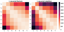
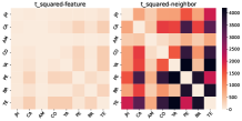
We first identify distribution shifts within both datasets. To assess concept shifts, we employ Hotelling’s T-squared statistics to measure the disparity between node distributions sharing the same class label. Our intuition is that if the nodes from the same class in two graphs have significantly different distributions, we can claim the graphs exhibit a concept shift with different feature/structure-label mappings. We present the pairwise T-squared scores comparing node feature embeddings and neighborhood representations of nodes from the first class across subgraphs for Facebook-100 (Figure 4 (a)) and OGB-elliptic (Figure 4 (a)). A higher T-squared score indicates a greater dissimilarity between the two distributions. In Figure 4, we observe that the subgraphs within Facebook-100 experience significantly less extent shift in node features compared to neighborhood representations, suggesting a dominance of neighborhood shift (def. concept shift-A). For OGB-elliptic, we initially notice a gradual increase in the T-squared score across the axis, indicating that the distribution shift intensifies over time. Additionally, we observe that it experiences concept shift-A and concept shift-X more evenly, with the latter slightly more dominant.
 |
 |
| (a) OGB-elliptic | (b) Facebook-100 |
| h-feat | qrt-feat | full-feat | ||
|---|---|---|---|---|
| best GNN | ERM | 40.7811.45 | 21.683.81 | 41.760.63 |
| IRM | 38.102.54 | 12.864.47 | 13.166.42 | |
| EERM | 35.1515.09 | 39.4610.48 | 54.710.74 | |
| CIT | 30.8325.93 | 18.3711.45 | 38.281.70 | |
| FLOOD | 47.224.16 | 35.5921.58 | 42.179.55 | |
| StableGL | 32.8312.24 | 28.5620.37 | 45.120.77 | |
| DeCaf | 57.2413.75 | 49.002.61 | 54.111.14 | |
| H2GCN | ERM | 49.383.44 | 31.721.60 | 66.591.86 |
| IRM | 51.178.82 | 33.574.78 | 62.041.45 | |
| EERM | 49.043.54 | 30.041.72 | 65.671.62 | |
| CIT | 54.333.90 | 30.283.96 | 64.782.64 | |
| FLOOD | 47.184.97 | 29.561.13 | 64.650.79 | |
| StableGL | 39.992.97 | 37.445.21 | 63.064.10 | |
| DeCaf | 55.925.20 | 44.961.78 | 67.021.12 |
For facebook-100, we report the F1-score of DeCaf in comparison with the baselines on each of the test graphs in Table 3.2. For each method, we use SGC, GCN, GAT, and H2GCN as baselines, and only report the results of the best-performed GNN selected with the validation set. We provide the results when using the first set of training graphs. Complete results are provided in Appendix 11. We observe that DeCaf significantly outperforms best baselines with an average improvement of 3.8%, showing that DeCaf enhances the generalizability of GNNs across different domains.
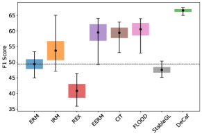
For OGB-elliptic, we plot the distribution of the F1 score averaged on all of the test graph snapshots with SGC as the backbone in Figure 3. The rectangles represent the standard deviation, and the error bars illustrate the range of data samples. The dashed line shows the mean F1 score of the ERM method. As shown, DeCaf significantly outperforms all baselines with a higher mean F1 score while demonstrating more stable performance, indicated by a smaller standard deviation, showing its ability to handle potentially more complex temporal shifts.
We also note that unlike other datasets, where in most cases the baseline graph OOD methods the baseline graph OOD methods either slightly improve or achieve comparable performance as ERM, on facebook-100 and OGB-elliptic, most of them degrade the performance significantly. The reasons behind this could be that the false assumptions made by those methods fail to apply to the distribution shifts in real-life scenarios and the over-confidence brought by their strategies could further degrade the generalizability of the model.
3.4 The impact of confounder effect (RQ3)
We create three synthetic graphs, h-feat, qtr-feat, and full-feat, to simulate scenarios with and without confounder effects between node features and neighborhood representations. h-feat is created such that the node features and neighborhood representations are dependent and act as confounders to each other. In contrast, full-feat and qtr-feat are designed so that these elements are independent, with no confounder effects. Details for creating these datasets are provided in Appendix 10.4.
We compare our model against baselines on the three synthetic datasets. We report the results of the best-performed one between SGC, GCN, GAT selected with the validation set. We also incorporate H2GCN to address potential heterophily in these datasets. Besides, H2GCN separately models node features and neighborhood representations, making its performance on a useful benchmark for our decoupling framework. We present the average Macro-F1 scores in Table 4. We report the results for the best-performed one among SGC, GCN, and GAT due to page limitation, please refer to Table 12 in Appendix for the full results. For qtr-feat and full-feat, where node features and neighborhood representations are independent, employing H2GCN on ERM significantly improves the Macro-F1 score compared to other GNN models. However, in h-feat, where node features and neighborhood representations are correlated, the gains are modest and are outperformed by our model with any GNN backbone. This suggests that while the separate modeling approach of H2GCN can mitigate distribution shifts, it falls short in addressing confounder effects, thus underperforming when node features and neighborhood representations are correlated.
4 Conclusion
In this paper, we introduce a causal decoupling framework to improve out-of-distribution generalization on node classification. We develop a comprehensive theoretical foundation to show that, by independently estimating the treatment effects of node features and neighborhood representations, the casual decoupling framework is robust when dealing with different types of distribution shifts. Following this theoretical basis, we also propose an implementable end-to-end framework, DeCaf, that leverages casual inference technologies to estimate the decoupled representations and make final predictions. We demonstrate the effectiveness and the power of DeCaf for node classification on both real-world datasets and synthetic datasets under different types of distribution shifts.
References
- [1] Zonghan Wu, Shirui Pan, Fengwen Chen, Guodong Long, Chengqi Zhang, and Philip S. Yu. A comprehensive survey on graph neural networks. IEEE Transactions on Neural Networks and Learning Systems, 32(1):4–24, January 2021.
- [2] Yang Liu, Xiang Ao, Fuli Feng, Yunshan Ma, Kuan Li, Tat-Seng Chua, and Qing He. Flood: A flexible invariant learning framework for out-of-distribution generalization on graphs. In KDD, KDD ’23, page 1548–1558, New York, NY, USA, 2023. Association for Computing Machinery.
- [3] Martin Arjovsky, Léon Bottou, Ishaan Gulrajani, and David Lopez-Paz. Invariant risk minimization, 2020.
- [4] Haoyue Bai, Rui Sun, Lanqing Hong, Fengwei Zhou, Nanyang Ye, Han-Jia Ye, S.-H. Gary Chan, and Zhenguo Li. Decaug: Out-of-distribution generalization via decomposed feature representation and semantic augmentation. Proceedings of the AAAI Conference on Artificial Intelligence, 35(8):6705–6713, May 2021.
- [5] David Krueger, Ethan Caballero, Jörn-Henrik Jacobsen, Amy Zhang, Jonathan Binas, Rémi Le Priol, and Aaron C. Courville. Out-of-distribution generalization via risk extrapolation (rex). CoRR, abs/2003.00688, 2020.
- [6] Shiori Sagawa, Pang Wei Koh, Tatsunori B. Hashimoto, and Percy Liang. Distributionally robust neural networks for group shifts: On the importance of regularization for worst-case generalization. CoRR, abs/1911.08731, 2019.
- [7] Zheyan Shen, Jiashuo Liu, Yue He, Xingxuan Zhang, Renzhe Xu, Han Yu, and Peng Cui. Towards out-of-distribution generalization: A survey. CoRR, abs/2108.13624, 2021.
- [8] Haotian Ye, Chuanlong Xie, Tianle Cai, Ruichen Li, Zhenguo Li, and Liwei Wang. Towards a theoretical framework of out-of-distribution generalization, 2021.
- [9] Shurui Gui, Xiner Li, Limei Wang, and Shuiwang Ji. Good: A graph out-of-distribution benchmark, 2022.
- [10] Felix Wu, Amauri Souza, Tianyi Zhang, Christopher Fifty, Tao Yu, and Kilian Weinberger. Simplifying graph convolutional networks. In Proceedings of the 36th International Conference on Machine Learning, volume 97 of Proceedings of Machine Learning Research, pages 6861–6871. PMLR, 09–15 Jun 2019.
- [11] P. M. Robinson. Root-n-consistent semiparametric regression. Econometrica, 56(4):931–954, 1988.
- [12] Jean Kaddour, Yuchen Zhu, Qi Liu, Matt J Kusner, and Ricardo Silva. Causal effect inference for structured treatments. In M. Ranzato, A. Beygelzimer, Y. Dauphin, P.S. Liang, and J. Wortman Vaughan, editors, Advances in Neural Information Processing Systems, volume 34, pages 24841–24854. Curran Associates, Inc., 2021.
- [13] Qitian Wu, Hengrui Zhang, Junchi Yan, and David Wipf. Handling distribution shifts on graphs: An invariance perspective. In International Conference on Learning Representations, 2022.
- [14] Donglin Xia, Xiao Wang, Nian Liu, and Chuan Shi. Learning invariant representations of graph neural networks via cluster generalization. In Thirty-seventh Conference on Neural Information Processing Systems, 2023.
- [15] Shengyu Zhang, Yunze Tong, Kun Kuang, Fuli Feng, Jiezhong Qiu, Jin Yu, Zhou Zhao, Hongxia Yang, Zhongfei Zhang, and Fei Wu. Stable prediction on graphs with agnostic distribution shifts. In Proceedings of The KDD’23 Workshop on Causal Discovery, Prediction and Decision, volume 218 of Proceedings of Machine Learning Research, pages 49–74. PMLR, 07 Aug 2023.
- [16] Qi Zhu, Natalia Ponomareva, Jiawei Han, and Bryan Perozzi. Shift-robust GNNs: Overcoming the limitations of localized graph training data. Advances in Neural Information Processing Systems, 34, 2021.
- [17] Qitian Wu, Yiting Chen, Chenxiao Yang, and Junchi Yan. Energy-based out-of-distribution detection for graph neural networks. In The Eleventh International Conference on Learning Representations, 2023.
- [18] Oleg Platonov, Denis Kuznedelev, Michael Diskin, Artem Babenko, and Liudmila Prokhorenkova. A critical look at the evaluation of gnns under heterophily: Are we really making progress?, 2024.
- [19] Jiong Zhu, Yujun Yan, Lingxiao Zhao, Mark Heimann, Leman Akoglu, and Danai Koutra. Generalizing graph neural networks beyond homophily. CoRR, abs/2006.11468, 2020.
- [20] Amanda L. Traud, Peter J. Mucha, and Mason A. Porter. Social structure of facebook networks. Physica A: Statistical Mechanics and its Applications, 391(16):4165–4180, August 2012.
- [21] Benedek Rozemberczki, Carl Allen, and Rik Sarkar. Multi-Scale attributed node embedding. Journal of Complex Networks, 9(2):cnab014, 05 2021.
- [22] Krikamol Muandet, David Balduzzi, and Bernhard Schölkopf. Domain generalization via invariant feature representation, 2013.
- [23] Kartik Ahuja, Karthikeyan Shanmugam, Kush R. Varshney, and Amit Dhurandhar. Invariant risk minimization games. CoRR, abs/2002.04692, 2020.
- [24] Petar Veličković, Guillem Cucurull, Arantxa Casanova, Adriana Romero, Pietro Liò, and Yoshua Bengio. Graph attention networks. In International Conference on Learning Representations, 2018.
- [25] Thomas N. Kipf and Max Welling. Semi-supervised classification with graph convolutional networks. CoRR, abs/1609.02907, 2016.
- [26] Haoyang Li, Xin Wang, Ziwei Zhang, and Wenwu Zhu. Ood-gnn: Out-of-distribution generalized graph neural network. IEEE Transactions on Knowledge and Data Engineering, 35(7):7328–7340, 2023.
- [27] Shaohua Fan, Xiao Wang, Chuan Shi, Peng Cui, and Bai Wang. Generalizing graph neural networks on out-of-distribution graphs. IEEE Transactions on pattern analysis and machine intelligence, 46, 2024.
- [28] Yongduo Sui, Xiang Wang, Jiancan Wu, Xiangnan He, and Tat-Seng Chua. Deconfounded training for graph neural networks. CoRR, abs/2112.15089, 2021.
- [29] Ying-Xin Wu, Xiang Wang, An Zhang, Xia Hu, Fuli Feng, Xiangnan He, and Tat-Seng Chua. Deconfounding to explanation evaluation in graph neural networks, 2022.
- [30] Yongqiang Chen, Yonggang Zhang, Yatao Bian, Han Yang, MA KAILI, Binghui Xie, Tongliang Liu, Bo Han, and James Cheng. Learning causally invariant representations for out-of-distribution generalization on graphs. In Advances in Neural Information Processing Systems, 2022.
- [31] Haoyang Li, Ziwei Zhang, Xin Wang, and Wenwu Zhu. Learning invariant graph representations for out-of-distribution generalization. In Advances in Neural Information Processing Systems, volume 35, pages 11828–11841. Curran Associates, Inc., 2022.
- [32] Ying-Xin Wu, Xiang Wang, An Zhang, Xiangnan He, and Tat-Seng Chua. Discovering invariant rationales for graph neural networks. CoRR, abs/2201.12872, 2022.
- [33] Davide Buffelli, Pietro Lio, and Fabio Vandin. Sizeshiftreg: a regularization method for improving size-generalization in graph neural networks. In Proceedings of the 36th International Conference on Neural Information Processing Systems, 2022.
- [34] Shaohua Fan, Xiao Wang, Chuan Shi, Kun Kuang, Nian Liu, and Bai Wang. Debiased graph neural networks with agnostic label selection bias. CoRR, abs/2201.07708, 2022.
- [35] Haoyang Li, Xin Wang, Ziwei Zhang, and Wenwu Zhu. Out-of-distribution generalization on graphs: A survey, 2022.
- [36] Kun Kuang, Ruoxuan Xiong, Peng Cui, Susan Athey, and Bo Li. Stable prediction across unknown environments. CoRR, abs/1806.06270, 2018.
- [37] Jianxin Ma, Peng Cui, Kun Kuang, Xin Wang, and Wenwu Zhu. Disentangled graph convolutional networks. In Kamalika Chaudhuri and Ruslan Salakhutdinov, editors, Proceedings of the 36th International Conference on Machine Learning, volume 97 of Proceedings of Machine Learning Research, pages 4212–4221. PMLR, 09–15 Jun 2019.
- [38] Yanbei Liu, Xiao Wang, Shu Wu, and Zhitao Xiao. Independence promoted graph disentangled networks. Proceedings of the AAAI Conference on Artificial Intelligence, 34(04):4916–4923, Apr. 2020.
- [39] James J. Heckman, John Eric Humphries, and Gregory Veramendi. Returns to education: The causal effects of education on earnings, health, and smoking. Journal of Political Economy, 126(S1):S197–S246, 2018.
- [40] Mattia C. F. Prosperi, Yi Guo, Matt Sperrin, James S. Koopman, Jae Min, Xing He, Shannan N. Rich, Mo Wang, Iain E. Buchan, and Jiang Bian. Causal inference and counterfactual prediction in machine learning for actionable healthcare. Nature Machine Intelligence, 2:369 – 375, 2020.
- [41] Liuyi Yao, Sheng Li, Yaliang Li, Mengdi Huai, Jing Gao, and Aidong Zhang. Representation learning for treatment effect estimation from observational data. In Advances in Neural Information Processing Systems, volume 31. Curran Associates, Inc., 2018.
- [42] Victor Chernozhukov, Denis Chetverikov, Mert Demirer, Esther Duflo, Christian Hansen, Whitney Newey, and James Robins. Double/debiased machine learning for treatment and causal parameters, 2017.
- [43] Alberto Abadie and Guido W. Imbens. Large sample properties of matching estimators for average treatment effects. Econometrica, 74(1):235–267, 2006.
- [44] Peter C. Austin. An introduction to propensity score methods for reducing the effects of confounding in observational studies. Multivariate Behavioral Research, 46(3):399–424, 2011. PMID: 21818162.
- [45] Donald B. Rubin. Using multivariate matched sampling and regression adjustment to control bias in observational studies. ETS Research Bulletin Series, 1978(2):i–33, 1978.
- [46] Yale Chang and Jennifer Dy. Informative subspace learning for counterfactual inference. Proceedings of the AAAI Conference on Artificial Intelligence, 31(1), Feb. 2017.
- [47] Donald B. Rubin. Matching to remove bias in observational studies. Biometrics, 29(1):159–183, 1973.
- [48] Jennifer L. Hill. Bayesian nonparametric modeling for causal inference. Journal of Computational and Graphical Statistics, 20(1):217–240, 2011.
- [49] Stefan Wager and Susan Athey. Estimation and inference of heterogeneous treatment effects using random forests. Journal of the American Statistical Association, 113(523):1228–1242, 2018.
- [50] Sören R. Künzel, Jasjeet S. Sekhon, Peter J. Bickel, and Bin Yu. Metalearners for estimating heterogeneous treatment effects using machine learning. Proceedings of the National Academy of Sciences, 116(10):4156–4165, 2019.
- [51] Michele Jonsson Funk, Daniel Westreich, Chris Wiesen, Til Stürmer, M. Alan Brookhart, and Marie Davidian. Doubly Robust Estimation of Causal Effects. American Journal of Epidemiology, 173(7):761–767, 03 2011.
- [52] Uri Shalit, Fredrik D. Johansson, and David Sontag. Estimating individual treatment effect: generalization bounds and algorithms, 2017.
- [53] Fredrik Johansson, Uri Shalit, and David Sontag. Learning representations for counterfactual inference. In Proceedings of The 33rd International Conference on Machine Learning, volume 48 of Proceedings of Machine Learning Research, pages 3020–3029, New York, New York, USA, 20–22 Jun 2016. PMLR.
- [54] Claudia Shi, David M. Blei, and Victor Veitch. Adapting neural networks for the estimation of treatment effects, 2019.
- [55] Susan Athey and Stefan Wager. Estimating treatment effects with causal forests: An application. Observational Studies, 5, 2019.
- [56] Ioana Bica, James Jordon, and Mihaela van der Schaar. Estimating the effects of continuous-valued interventions using generative adversarial networks. CoRR, abs/2002.12326, 2020.
- [57] Nathan Kallus. DeepMatch: Balancing deep covariate representations for causal inference using adversarial training. In Hal Daumé III and Aarti Singh, editors, Proceedings of the 37th International Conference on Machine Learning, volume 119 of Proceedings of Machine Learning Research, pages 5067–5077. PMLR, 13–18 Jul 2020.
- [58] Shonosuke Harada and Hisashi Kashima. Graphite: Estimating individual effects of graph-structured treatments. CoRR, abs/2009.14061, 2020.
- [59] Andrew McCallum, Kamal Nigam, Jason D. M. Rennie, and Kristie Seymore. Automating the construction of internet portals with machine learning. Information Retrieval, 3(2):127–163, 2000.
- [60] C. Lee Giles, Kurt D. Bollacker, and Steve Lawrence. Citeseer: an automatic citation indexing system. In Proceedings of the Third ACM Conference on Digital Libraries, DL ’98, page 89–98, New York, NY, USA, 1998. Association for Computing Machinery.
- [61] Oleksandr Shchur, Maximilian Mumme, Aleksandar Bojchevski, and Stephan Günnemann. Pitfalls of graph neural network evaluation, 2019.
- [62] Julian McAuley, Christopher Targett, Qinfeng Shi, and Anton van den Hengel. Image-based recommendations on styles and substitutes, 2015.
Appendix
1 Related work
1.1 OOD Generalization on Graphs
Abundant pioneer works [22, 23, 4, 5, 6, 7, 8] have been dedicated to addressing the out-of-distribution (OOD) generalization problem. The primary objective of OOD generalization is to train models within a specific domain and anticipate their robust generalization to test domains from potentially distinct distributions [8]. While most of these methods are tailored to deal with distribution shifts on tabular data or images, their performance is restricted when confronted with more complex data structures. With the success of Graph Neural Networks (GNNs) [24, 25], more recent research starts to address the OOD problem on graphs [26, 27, 28, 29, 30, 31, 32, 33, 34, 13, 2, 14, 15, 16]. OOD generalization on graphs is more intractable due to the non-euclidean nature of graph data structures and the subtlety of different types of distribution shifts [35].
One consensus of OOD generalization is that, when domain knowledge is unavailable, knowledge transfer to a new domain is impossible without structural assumption on data generation processes [13]. A general assumption made by most OOD generalization methods is that there exist “true” correlations between input data features and their labels. These correlations remain invariant across different domains, and they aim to identify these true connections while removing the spurious ones [35]. Most of the existing graph OOD generalization methods leverage this assumption in different manners or extend it to more specific forms. Approaches [26, 27, 34] backed by confounder balancing [36] from casual theories remove the correlations between casual and non-causal (spurious) aspects (in the forms of representations [26], subgraphs [27], or samples [34], etc.) such that the model can focus on the casual ones. Some methods [31, 32, 13, 2, 14, 15] leverage invariance principle [3] from causality and assumes that there exists a portion of information in the input (e.g., subgraphs) that is invariant to label predictions across different environments. This approach often requires access to multiple environments/domains during the training process, which are not always available. Structural causal graphs (SCGs) have also been used for assumptions in data generation processes [28, 29, 30]. They focus on making unbiased estimations of causal relationships via do-calculus [28] or back-door adjustments [29]. Zhu et al. [16] assume that training data are from a biased data generation process while test data are unbiased. Buffelli et al. [33] improves model generalization on smaller or larger test graphs by minimizing the discrepancy between the learned representation on the original graph and the coarsened graph.
Among the above-mentioned methods, most of them [26, 27, 28, 29, 30, 31, 32, 33] are tailored for graph-level or link-level tasks, and it is non-trivial to adapt them to node-level tasks. For the rest of the methods [34, 13, 2, 14, 15, 16] that can be applied on node-level tasks, an ego-net is often the starting point for any further actions to be taken (to generate an invariant subgraph, or to learn the invariant representation of it, etc). Current approaches involve aggregating a central node and its neighborhood into a unified representation (e.g., GCNs [25] or GATs [24]), but they tend to overlook and filter out potential complex dependencies (or independencies) between them. Certain GNNs such as H2GCN [19] can model the central node and its neighbors’ representations separately through the concatenation operation during the aggregation, but inferences on their relations are still missing. Disentangled graph learning [37, 38] investigates latent factors that may cause the formation of an edge between a node and its neighbors. This method can also improve the OOD generalizability of GNNs, but it focuses on explaining the existence of edges with node representations, which is fundamentally different from our focus.
1.2 Causal Effect Estimation
Estimating the causal effect of treatment plays a crucial role in many domains [39, 40]. With the presence of the confounder, two types of studies, dubbed randomized controlled trials (RCTs) and observational studies, are often conducted to achieve an unbiased estimation of casual effects [41]. Often, RCTs are expensive, unethical, or infeasible [41], leaving observational studies the only option. The challenges of observational studies are that the counterfactual samples are missing from observational data, and the estimation of counterfactual output is often biased due to the treatment selection bias caused by the confounder effect [42]. Traditional solutions include matching methods [43, 44, 45, 46, 47], tree-based methods [48, 49], and regression-based methods [50, 51]. Recently, representation learning methods [52, 41, 53, 54, 55, 56, 57] have also been widely studied and demonstrate impressive performance. The above-mentioned studies focus on binary or categorical treatments, which are difficult to apply when the treatments are real-valued and structured. GraphITE [58] is proposed to deal with graph-structured treatment, which mitigates observation biases by reinforcing the independence between the treatment and covariate representations in the notion of Hilbert-Schmidt Independence Criterion (HSIC). Robinson decomposition [12] is used to identify the distinct contribution of the treatment and the covariates and generalizes it such that the treatment can be vectorized to a continuous embedding.
2 Pseudo code
We provide the pseudo-code for DeCaf in Algorithm 1.
3 Important mathematical notations
We provide a summary of important mathematical notations in Table 5.
| Notation | Description |
|---|---|
| nodes, feature size, classes, hidden size | |
| , , | node feature vector, node feature of -th instance, node feature matrix |
| , , | node label vector, label of -th instance, node label matrix |
| , , | neighborhood representation, neighborhood representation, of -th instance, |
| neighborhood representation matrix | |
| unnormalized adjacency matrix | |
| GNN embedding layer, MLP layer | |
| parameters of | |
| , | hidden neighborhood representation of node , and its project to output space |
| confounder representation function for SCM-F and SCM-A | |
| parameters for | |
| treatment representation function for SCM-F and SCM-A | |
| parameters for | |
| confounder predicting function for SCM-F and SCM-A | |
| parameters for | |
| propensity feature function for SCM-F and SCM-A | |
| parameters for | |
| , | counterfactual node feature and neighborhood representation |
4 Discussion on spillover effect
Assumption 4.
The Law of Large Numbers is invoked, ensuring that the sample size is sufficiently large such that the observed distribution of the random variable z remains stable and converges towards its theoretical distribution.
5 Analysis on distribution shifts
Proposition 1.
Under covariate shift, the correlation between and shifts (e.g. or ). Consequently, the conditional distribution of given both and shifts (e.g. ). However, the conditional distribution of given alone remain invariant (e.g. ).
Proof.
Under covariate shift, we have:
while the transformation matrices and bias vectors for generating , , and remain the same between training and testing datasets:
The generation processes are:
where is defined as:
Given that changes, the marginal distribution of changes accordingly:
Since is an aggregation of transformed neighbors’ latent vectors , and changes, the distribution of also changes:
To show that the joint distribution changes, consider that is derived from through a different transformation and aggregation function. Since and are both functions of , any change in the distribution of will induce changes in both and . Given that and change independently due to the change in , the joint distribution must also change because the dependencies between and are functions of :
This implies that:
The generation process for is:
Since and are the same across training and testing, and influences and through , , , and , the change in affects and . Consequently, the joint distribution changes:
Thus, the conditional distribution:
Since and and are invariant, the conditional distribution remains invariant:
Given that and and are invariant, the conditional distribution also remains invariant:
∎
Proposition 2.
Under concept shift-F, the dependencies between and shifts (e.g. or ), and the conditional distribution of given shifts (e.g. ). Consequently, the conditional distribution of given both and shifts (e.g. ). However, the conditional distribution of given alone remain invariant (e.g. ).
Proof.
Under concept shift-F, we have:
while the transformation matrices and bias vectors for generating change, but those for and remain the same between training and testing datasets:
The generation processes are:
where is defined as:
Given that remains the same, the marginal distribution of does not change:
However, the change in the transformation matrix and bias vector implies that the marginal distribution of changes:
Since is an aggregation of transformed neighbors’ latent vectors , and the generation process for remains unchanged, the joint distribution changes due to the change in :
This implies that:
The generation process for is:
Since and are the same across training and testing, and influences through , the change in affects the joint distribution :
Thus, the conditional distribution:
The change in the joint distribution implies a change in the joint distribution since depends on both and :
Thus, the conditional distribution:
Since and are both derived from through invariant transformation matrices and bias vectors, and remains the same, the joint distribution remains unchanged:
Thus, the conditional distribution:
∎
Proposition 3.
Under concept shift-A, the dependencies between and shifts (e.g. or ), and the conditional distribution of given shifts (e.g. ). Consequently, the conditional distribution of given both and shifts (e.g. ). However, the conditional distribution of given alone remain invariant (e.g. ).
Proof.
Under concept shift-A, we have:
while the transformation matrices and bias vectors for generating change, but those for and remain the same between training and testing datasets:
The generation processes are:
where is defined as:
Given that remains the same, the marginal distribution of does not change:
However, the change in the transformation matrices and implies that the marginal distribution of changes:
Since is an aggregation of transformed neighbors’ latent vectors , and the generation process for changes, the joint distribution changes due to the change in :
This implies that:
The generation process for is:
Since and are the same across training and testing, and influences through and , the change in and affects the joint distribution :
Thus, the conditional distribution:
Since and are both derived from through invariant transformation matrices and bias vectors, and remains the same, the joint distribution remains unchanged:
Thus, the conditional distribution:
The change in the joint distribution implies a change in the joint distribution since depends on both and :
Thus, the conditional distribution:
∎
6 Important assumptions for CATE estimation
Assumption 5.
(SUTVA). The potential outcomes of any unit do not vary with the treatment assigned to other units, and, for each unit, there are no different forms or versions of each treatment level, which leads to different potential outcomes.
We discuss the reasonableness of this assumption in section 2.1.
Assumption 6.
(Consistency). The potential outcome of treatment equals the observed outcome if the actual treatment received is .
Assumption 7.
(Ignorability). Given pretreatment covariate , the outcome variable and is independent of treatment assignment, i.e. .
This assumption is also called “no unmeasured confounder”. This assumption is automatically satisfied with the “close-world assumption” made in learning a machine learning model, which implicitly assumes that the input data encompasses the necessary information for making accurate predictions, as we explain in section 2.1. In our case, it implies that no other confounders besides and that affect the output should exist.
Assumption 8.
(Positivity). For any set of covariates , the probability to receive any treatment is positive, i.e., .
7 Derivation of the prediction function of SGC
A typical SGC makes predictions with the classifier:
| (15) |
where is the “normalized” adjacency matrix , , is the degree matrix of , is the number of layers, is the parameterized weights of each layer into a single matrix: . Note that the above equation 15 averages the representation of all nodes at each hop, so the effect of the central node is diminished when its neighbor size is large. Alternatively, we can assign a fixed weight to the central node, and the rest is shared by the neighboring nodes during the aggregation process, so the in equation 15 is replaced by , where:
| (16) |
where and are diagonal matrix such that and . The new prediction function is then expressed as:
| (17) | ||||
| (18) |
Inside , the first term models the contribution of the neighborhood nodes’ representation (excluding central node) on , we call it ; similarly, the second term models the contribution of the features of the central node and we call it . Note that the magnitudes of the diagnal matrixes of and are scaled by the parameter . We can further rewrite Equation 18 in the unscaled form:
| (19) |
where can be viewed as , and can be viewed as , which aligns with asssumtion 2.
8 Dual Casual Decomposition
We aim to learn two sets of for the two casual models SCM-F and SCM-A. We denote them as and , separately. Each casual model is also associated with a set of , denoted as and . Unlike SIN, which learns all model parameters within the two-stage training procedure, we allow the model to learn , , and with shared parameters beforehand. Since , , and are all functions of the neighborhood representation , whose value is determined with a -layer GNN model that generates a neighborhood representation by aggregating the embedding of nodes in -hop neighborhood without including the central node.
We then map the GNN embedding to the space of with an MLP layer that follows .
The parameters of and , , are learned with the goal of minimizing: . As the ground truth is not available, while is available, we thus apply on both sides and minimizing the following cross entropy function instead:
| (20) |
We apply this alternation for the rest of the training process. With the optimized , we first assign the learned neighborhood representation to , such that . Without losing generalizability, we assign , as the same as . We then estimate , with the optimized . , , and remain fixed values in the rest of the learning process:
We learn the remaining parameters for each casual model. For SCM-A, we follow the two-stage procedure:
Stage 1: Learn parameter of to minimize the cross-entropy loss as following:
Stage 2: Learn parameter for and for with the objectives:
| (21) |
For SCM-F, stage 1 is no longer necessary as is fixed as . We only need to learn parameter for and for with the objectives:
| (22) |
We follow the alternating optimization process in [12] which updates more frequently than to achieve a more stabilized training process.
9 Complexity analysis
Consider a graph with nodes and edges, and an average degree . A Graph Neural Network (GNN) with layers computes embeddings with a time and space complexity of . When obtaining the GNN embedding, DeCaf performs one encoder computation per update step. During training, five distinct encoders are learned for causal models, each with a time complexity of per update step. Therefore, the overall time complexity is .
We compare the complexity and requirements of DeCaf with other methods in Table 6. For EERM and FLOOD, is the number of augmented training environments. For CIT, is the number of clusters and is the probability of transfer. As it shows, DeCaf has competitive complexity, while having the least restrictive requirements, making it applicable to a wide range of scenarios.
| Method |
Tailored
for graphs |
Multiple
training envs |
Training envs
augmentation |
Access to test
distributions |
Test-time
training |
Complexity |
|---|---|---|---|---|---|---|
| ERM | N/A | N/A | N/A | N/A | N/A | |
| IRM | ✗ | Required | Not Required | Not Required | Not Required | |
| REX | ✗ | Required | Not Required | Not Required | Not Required | |
| EERM | ✓ | Not Required | Required | Not Required | Not Required | |
| CIT | ✓ | Not Required | Not Required | Not Required | Not Required | |
| FLOOD | ✓ | Required | Not Required | Not Required | Required | |
| SR-GNN | ✓ | Not Required | Not Required | Required | Not Required | |
| DeCaf | ✓ | Not Required | Not Required | Not Required | Not Required |
10 Datasets and Setup
10.1 Hyperparameter Setup
The hidden size of the backbone GNNs of all methods is searched from 8, 16, 32, 64, 128, the number of heads for GAT is searched from 4, 8, and the number of layers is 2. We use Adam as the optimizer with a learning rate of 1e-3 and weight decay of 1e-5. For methods with penalty weights, we searched from different values centered on their default value. For instance, for IRM, the default penalty weight is 1e5, we then conduct our search on 1e2, 1e3, 1e4, 1e5, 1e6, 1e7, 1e8. We follow the default setting for other hyperparameters, such as the number of augmented views. All experiments are conducted on an NVIDIA GeForce RTX 3090 GPU with 24GB memory.
10.2 Soft label leave-out setting
In our experiments, if we have 6 classes and the training set has from the first two classes, from the second two classes, and from the last two classes. Then, the validation set owns from the first two classes, from the second two classes, and from the last two classes. Test set owns from the first two classes, from the second two classes, and from the last two classes.
| Cora | Citeseer | Amazon-photo | Coauthor-CS | Squirrel | Roman-empire | Tolokers | |
| # Node | 2,708 | 3,327 | 7,650 | 18,333 | 2,223 | 22,662 | 11,758 |
| # Edge | 5,278 | 4,552 | 119,081 | 81,894 | 23,499 | 32,927 | 259,500 |
| # Class | 7 | 6 | 8 | 15 | 5 | 18 | 2 |
| # Feat | 1433 | 3703 | 745 | 6,805 | 2,089 | 300 | 10 |
| Metric | Marco-F1 | Marco-F1 | Marco-F1 | Marco-F1 | Marco-F1 | Marco-F1 | F1 score |
| Johns Hopkins | Caltech | Amherst | Bingham | Duke | Princeton | WashU | |
|---|---|---|---|---|---|---|---|
| # Node | 5,180 | 769 | 2,235 | 10,004 | 9,895 | 6,596 | 7,755 |
| # Edge | 373,172 | 33,312 | 181,908 | 725,788 | 1,012,884 | 586,640 | 735,082 |
| Positive rate | 43% | 53% | 36% | 40% | 39% | 37% | 38% |
| Brandeis | Carnegie | Penn | Brown | Texas | Cornell5, | Yale | |
| # Node | 3,898 | 6,637 | 41,554 | 8,600 | 31,560 | 18,660 | 8,578 |
| # Edge | 275,134 | 499,934 | 2,724,458 | 769,052 | 2,439,300 | 1,581,554 | 810,900 |
| Positive rate | 30% | 47% | 43% | 32% | 37% | 37% | 35% |
| Time slot | 1-6 | 7-12 | 13-18 | 19-24 | 25-30 | 31-36 | 37-43 |
|---|---|---|---|---|---|---|---|
| # Node | 28,571 | 18,525 | 25,985 | 14,337 | 24,878 | 25,920 | 29,684 |
| # Edge | 33,835 | 19,613 | 29,274 | 15,296 | 28,223 | 29,689 | 33,659 |
| Positive rate | 11% | 22% | 12% | 23% | 12% | 10% | 3% |
| h-feat | qtr-feat | full-feat | |
| # Node | 8,000 | 8,000 | 8,000 |
| # Edge | 404,597 | 1,487,637 | 35,850 |
| # Class | 4 | 4 | 4 |
| # Feat | 8 | 4 | 16 |
| Training | Johns Hopkins + Caltech + Amherst | Bingham + Duke + Princeton | WashU + Brandeis + Carnegie | ||||||
|---|---|---|---|---|---|---|---|---|---|
| Test | Penn | Brown | Texas | Penn | Brown | Texas | Penn | Brown | Texas |
| ERM | 49.231.72 | 49.680.93 | 48.570.21 | 51.424.25 | 51.451.48 | 47.374.78 | 47.345.48 | 48.082.51 | 48.364.30 |
| IRM | 35.262.40 | 46.925.66 | 36.861.64 | 42.121.99 | 51.340.90 | 41.574.31 | 50.161.30 | 49.623.32 | 46.415.28 |
| REX | 44.776.48 | 42.657.34 | 44.058.88 | 43.775.72 | 47.265.75 | 44.367.82 | 39.678.59 | 44.656.67 | 40.287.59 |
| EERM | 22.6222.91 | 49.441.92 | 49.121.71 | 18.9118.99 | 45.953.74 | 47.831.17 | 24.4024.62 | 47.582.91 | 51.271.04 |
| CIT | 44.666.65 | 45.266.21 | 42.108.97 | 45.826.46 | 48.621.88 | 39.794.74 | 37.996.54 | 39.666.58 | 39.886.27 |
| FLOOD | 42.375.06 | 41.485.28 | 40.825.94 | 46.997.48 | 47.285.61 | 44.485.22 | 41.217.68 | 46.248.52 | 40.166.01 |
| StableGL | 44.546.58 | 45.646.25 | 43.755.65 | 46.948.54 | 47.774.79 | 47.515.94 | 38.318.42 | 43.224.50 | 37.864.75 |
| DeCaf | 55.310.40 | 53.310.11 | 53.560.19 | 54.590.35 | 53.480.15 | 53.120.19 | 54.441.18 | 53.020.36 | 53.050.86 |
| h-feat | qrt-feat | full-feat | ||
| SGC | ERM | 47.410.25 | 48.621.88 | 48.570.21 |
| IRM | 33.781.41 | 33.360.70 | 33.041.40 | |
| EERM | 38.148.25 | 37.865.15 | 39.747.09 | |
| CIT | 21.1121.33 | 36.410.45 | 49.121.71 | |
| REX | 32.871.12 | 33.850.50 | 34.470.82 | |
| FLOOD | 39.538.83 | 37.264.82 | 39.136.39 | |
| StableGL | 41.798.86 | 38.305.60 | 41.226.30 | |
| DeCaf | 55.310.40 | 53.160.17 | 53.560.19 | |
| GCN | ERM | 43.121.84 | 49.680.93 | 43.791.36 |
| IRM | 34.030.94 | 32.900.60 | 32.471.16 | |
| EERM | 43.246.52 | 42.657.34 | 38.605.26 | |
| CIT | 22.7923.15 | 49.441.92 | 40.815.74 | |
| REX | 33.101.60 | 35.622.60 | 34.490.89 | |
| FLOOD | 38.586.60 | 40.076.76 | 38.586.57 | |
| StableGL | 42.126.44 | 44.774.78 | 43.755.65 | |
| DeCaf | 53.570.98 | 53.310.11 | 52.160.45 | |
| GAT | ERM | 49.231.72 | 47.341.25 | 46.131.54 |
| IRM | 35.262.40 | 46.925.66 | 36.861.64 | |
| EERM | 44.776.48 | 41.943.92 | 44.058.88 | |
| CIT | 22.6222.91 | 39.044.31 | 34.662.32 | |
| REX | 44.666.65 | 45.266.21 | 42.108.97 | |
| FLOOD | 42.375.06 | 41.485.28 | 40.825.94 | |
| StableGL | 44.546.58 | 45.646.25 | 41.886.88 | |
| DeCaf | 51.840.88 | 52.290.56 | 50.680.63 | |
| H2GCN | ERM | 49.383.44 | 31.721.60 | 66.591.86 |
| IRM | 51.178.82 | 33.574.78 | 62.041.45 | |
| EERM | 49.043.54 | 30.041.72 | 65.671.62 | |
| CIT | 54.333.90 | 30.283.96 | 64.782.64 | |
| FLOOD | 47.184.97 | 29.561.13 | 64.650.79 | |
| StableGL | 39.992.97 | 37.445.21 | 63.064.10 | |
| DeCaf | 55.925.20 | 44.961.78 | 67.021.12 |
10.3 Real-word datasets
We provide the statistics of single-graph datasets in Table 7. Cora [59], Citeseer [60], and Coauthor-CS [61] are citation networks. Amazon-photo [62] is a co-purchase network where nodes represent goods for sale on e-commerce websites. Squirrel, Roman-empire, and Tolokers are heterophilous networks created by Platonov [18] et al. Squirrel is a Wikipedia network, Roman-empire is created based on the Roman Empire article from English Wikipedia, and Tolokers is created based on data from the Toloka crowdsourcing platform, where the nodes represent tolokers (workers).
Facebook-100 [20] contains 100 social networks collected from universities in the United States. Each node represents a student and the goal is to predict the gender of each student. We provide the statistics of sub-datasets we use in Table 8.
OGB-elliptic [21] is a dynamic financial network dataset that contains in total of 43 graph snapshots from different time steps. Each node represents a Bitcoin transaction, and the goal is to detect illicit transactions. We group all 43 snapshots into 7 timeslots and provide statistics for each timeslot in Table 9.
10.4 Synthetic datasets
We create three synthetic graphs to simulate the situations where node features and neighborhood representation are dependent or independent of each other. For each graph, we randomly sample instances of with 16 features from a multivariate normal distribution. We generate node features, labels, and adjacency matrices based on the data generation process in assumption 1. By posing different constraints on , , , and , we can control the dependence/ independence between node features and neighborhood representation, and their contributions to the labels. Statistical details of these datasets are shown in Table 10.
h-feat: When can only “observe” half of the elements of and can fully observe , node features and neighborhood representation are correlated with each other, and each of them can reveal extra information about node label. To do so, we assign as a matrix with its first rows as an identical matrix, and the rest rows are all zeros, such that the second half elements of do not participate in the construction of . We assign and to be the same size and value as , which is guaranteed to be a non-trivial transformation of .
qtr-feat: When “observe” quarter of the elements of and can observe the rest three fourth, node features and neighborhood contributes to the prediction of node labels independently. We assign as a matrix with its first rows as an identical matrix, and the rest rows are all zeros. We assign and to be the same size and value as , except with the first rows replaced by all zeros.
full-feat: We create another graph where node features and neighborhoods contribute to the prediction of node labels independently in an alternative way. First, we make fully observe by assigning it as a identical matrix; then by assigning and as zeros, we create completely random edges. We slightly modify equation 2 to be , where is the mean embedding of neighboring nodes of node , such that the neighborhood representation can directly affect node labels.
11 Complete results
We report the complete results on facebook-100 when different sets of training graphs are used in Table 11. With different training sets, the proposed DeCaf achieves the best classification results over three different test sets compared with state-of-the-art OOD generalization methods.
12 Limitations
This paper focuses on homogeneous graphs with limited node and edge types. In the future, we plan to extend the method to heterogeneous graphs with more diverse node relations and neighborhood patterns. This extension will broaden the applications of our method to domains such as social networks, healthcare, and biological networks, where heterogeneity can provide rich information for making predictions.
13 Broader Impacts
DeCaf improves the generalizability of the GNN, helping it learn a faithful mapping between inputs and outputs that captures true correlations. This is crucial for critical domains vulnerable to security issues, such as cybersecurity, finance, and healthcare. Learning a robust and generalizable model under potential distribution shifts is essential for these domains.