Advancing Hybrid Quantum Neural Network for Alternative Current Optimal Power Flow

Abstract

Optimal Power Flow (OPF) is essential for efficient planning and real-time operation in power systems but is NP-hard and non-convex, leading to significant computational challenges. Neural networks (NNs) offer computational speedups in solving OPF but face issues like dependency on large datasets, scalability limitations, and inability to enforce physical constraints, compromising solution reliability. To overcome these limitations, this paper proposes hybrid Quantum Neural Networks (QNNs) that integrate quantum computing principles into neural network architectures. Leveraging quantum mechanics properties such as superposition and entanglement, QNNs can capture complex input-output relationships more effectively and learn from small or noisy datasets. To further enhance the performance of QNNs and explore the role of the classical (non-quantum) components in hybrid architectures, we apply residual learning and incorporate physics-informed layers into the hybrid QNN designs. These techniques aim to improve training efficiency, generalization capability, and adherence to physical laws. Simulation results demonstrate that these enhanced hybrid QNNs outperform conventional NNs in solving OPF problems, even when trained on imperfect data. This work provides valuable insights into the design and optimization of hybrid QNNs, highlighting their potential to address complex optimization challenges in power systems.

I Introduction

Optimal Power Flow (OPF) is a critical optimization problem integral to the operations and strategic planning of various stakeholders—including system operators and electricity market participants—for the efficient and reliable planning and real-time control of power systems. This pervasive reliance underscores OPF’s centrality in power systems; in the United States alone, OPF influences economic activities exceeding ten billion dollars annually [1].

One of primary objective of OPF is to minimize operational costs while satisfying physical constraints such as line capacities and bus voltages by determining the optimal power generation setpoints. However, the OPF problem is both NP-hard and non-convex, resulting in significant convergence challenges and protracted computational times for most solvers [2]. Furthermore, OPF must be computed repeatedly in many application scenarios, including electricity market clearing and bidding strategy determination, underscoring the necessity for fast and accurate OPF solutions. To address these challenges and ensure rapid computation with convergence guarantees, a substantial body of literature focuses on deriving approximations of the AC-OPF problem, with the linearized DC-OPF being one of the most prevalent methods [3].

In recent years, there has been a keen interest in employing machine learning methods, particularly neural networks (NNs), to estimate solutions of the AC-OPF problem [4, 5]. Compared to traditional methods, NNs demonstrate strong performance in learning non-convex functions and have exhibited computational speedups ranging from 100 to 1,000 times [5]. Despite their substantial potential, NN approaches still face significant challenges for real-world implementation. First, the performance of NNs in solving OPF heavily relies on the training dataset, which needs to be sufficiently large and of high quality; thus, they may suffer from typical machine learning issues such as data inadequacy or data loss in most available datasets. Second, the computational complexity of NNs escalates rapidly for larger-scale systems. As the dimensionality of input and output variables increases, NNs require more neurons and layers to capture the system’s characteristics, complicating hyperparameter tuning and demanding substantial computational resources. Last but not least, NNs disregard the underlying physical laws of OPF and are unable to enforce constraints on their solutions. Consequently, the solutions provided by NNs may not be reliable, as compliance with security constraints for line capacities and bus voltages is not guaranteed.

To overcome these challenges posed by classical neural networks in solving OPF problems, quantum neural networks (QNNs) have emerged as a promising alternative by integrating quantum computing principles into neural network architectures. QNNs, constructed from layers of quantum gates, belongs to gate-based quantum computing (GQC), which performs computations using quantum gates and discrete time steps, facilitating the simulation of specific computational processes. They possess the capability to explore high-dimensional feature spaces using a limited number of quantum resources, potentially leading to superior performance in practical applications [6]. The unique properties of quantum mechanics—namely superposition and entanglement—enable QNNs to capture complex relationships between inputs and outputs more effectively than classical NNs. Furthermore, the inherent probabilistic nature of quantum phenomena allows QNNs to learn from low quality datasets that is either small or noisy [7]. This advantage not only enhances the training process but also mitigates common data scarcity concerns in power system applications, positioning QNNs as promising candidates for scenarios where data is limited or expensive to obtain. In [8], QNNs have been applied to solve OPF problems, with simulation results demonstrating that QNN shows better performance in generalization and also dealing with noisy training data.

Despite these initial successes, QNNs have not yet been systematically explored for OPF solution. At the beginning of the century, it has been acknowledged that not all components of a QNN architecture need to be quantum for advantages to surface [9]. Much past literature [9, 10] has also demonstrated that a full QNN has no advantage over a hybrid quantum network that is a mix of quantum and classical components may, in fact, produce worse results. In such context, the classical (non-quantum) components in QNNs have significant roles in interacting with the quantum part, though the performance of such components is not fully understood. Therefore, this paper seeks to explore the design of the classical components and their interactive relation between the classical and quantum components in a hybrid QNN to improve its performance in solving specific tasks like AC-OPF problems.

The contributions of this paper are as follows:

1. Development of Enhanced Hybrid Quantum Neural Networks: We develop two hybrid quantum neural networks featuring different residual learning architectures. The proposed QNNs exhibit accelerated training processes and superior generalization performance compared to standard QNNs, demonstrating lower test errors than classical neural networks.

2. Integration of Physics-Informed Layers: We integrate a physics-informed layer into the QNN to incorporate fundamental physical laws and enforce compliance with security network constraints. This integration enhances the reliability and feasibility of the solutions by ensuring they adhere to essential operational limitations.

The rest of the paper is constructed as follows: The formulation of the AC-OPF problem along with its Karush-Kuhn-Tucker (KKT) conditions are presented in Section II. The the fundamentals and specific designs of quantum neural networks, including the implemented advanced techniques such as residual learning and physics-informed neural networks are introduced in Section III. The numerical results comparing the proposed approach with benchmark neural networks are shown in Section IV, highlighting the performance improvements. The paper is concluded in Section V, summarizing the key findings and suggesting directions for future research.

II Problem formulation

The AC-OPF problem is an optimization problem for ISO to schedule and dispatch resources in both day-ahead and real-time stages. According to the operation requirements, the objective of AC-OPF may be multiple, including generation cost minimization, line loss minimization, etc. The paper uses the typical objective of minimizing the total cost of active power generation. The AC-OPF problem model in compact form is presented as (1).

$$\min_{\mathbf{v},\mathbf{G}} \ \mathbf{c}^{T}\mathbf{G}$$ (1a)

s.t. $$\ \mathbf{v}^{T}\mathbf{L}_{l}\mathbf{v}={a}_{l}^{T}\mathbf{G}+{b}_{l}^{T}\mathbf{D},\quad l=1:L:\lambda_{l}$$ (1b)

$$\ \mathbf{v}^{T}\mathbf{M}_{m}\mathbf{v}\leq{d}_{m}^{T}\mathbf{D}+f_{m},\quad m=1:M:\mu_{m}$$ (1c)

In the optimization problem above, $\mathbf{c}^{T}$ is the combined linear cost terms for the active and reactive power generations, $\mathbf{G}=\begin{bmatrix}\mathbf{P}_{g}^{T},\mathbf{Q}_{g}^{T}\end{bmatrix}^{T}$, $\mathbf{D}=\begin{bmatrix}\mathbf{P}_{d}^{T},\mathbf{Q}_{d}^{T}\end{bmatrix}^{T}$. ${\mathbf{v}}=\begin{bmatrix}(\mathbf{v}^{r})^{T},(\mathbf{v}^{i})^{T}\end{bmatrix}^{T}$ is the voltage vector contains both the real and imagination part of voltage at all buses. $\mathbf{L}$ and $\mathbf{M}$ are combined vectors that stand for expressions of multiple constraints. ${a}_{l}$ and ${b}_{l}$ are vectors mapping generation and demands to the corresponding buses. $d_{m}$ is the vector mapping active and reactive power of demand in $\mathbf{D}$ to corresponding constraints. $f_{m}$ stands for vectors of bounded values for voltage and line flows. $\lambda_{l}$ and $\mu_{m}$ are dual variables for constraints. Please refer to the Appendix. A for further details.

In the proposed model, the objective in (1a) is to minimize the cost of power generation, subject to compact form constraints of (1b) and (1c). Constraint (1b) denotes all equality constraints, including $2N_{b}$ constraints for bus power injection and $1$ constraints for angle reference of the slack bus. (1c) stands for all inequality constraints, including $4N_{g}$ constraints for optimal power generation, $2N_{b}$ constraints for bus voltage, and $N_{l}$ constraints for line current flow. Based on the optimization above, the Lagrangian function for the AC-OPF can be formulated as (2).

$$\begin{array}[]{lrl}\mathcal{L}(\mathbf{x},\lambda,\mu,\mathbf{D})&=\mathbf{c}^{T}\mathbf{G}+\sum_{l=1}^{L}\lambda_{l}\left(\mathbf{v}^{T}\mathbf{L}_{l}\mathbf{v}-\mathbf{a}_{l}^{T}\mathbf{G}-\mathbf{b}_{l}^{T}\mathbf{D}\right)\\ &\quad+\sum_{m=1}^{M}\mu_{m}\left(\mathbf{v}^{T}\mathbf{M}_{m}\mathbf{v}-\mathbf{d}_{m}^{T}\mathbf{D}-f_{m}\right)\end{array}$$ (2)

Given the optimization problem and its Lagrangian function, the KKT conditions for the AC-OPF are presented in (3)-(9), where the stationarity condition is given in (3) and (4), the complementary slackness condition is given by (5), and dual feasibility is given by (6).

$$\mathbf{c} =\sum_{l=1}^{L}\lambda_{l}\mathbf{a}_{l}$$ (3)

$$\left(\sum_{l=1}^{L}\lambda_{l}\mathbf{L}_{l}+\sum_{m=1}^{M}\mu_{m}\mathbf{M}_{m}\right) =0$$ (4)

$$\mu_{m}\left(\mathbf{v}^{T}\mathbf{M}_{m}\mathbf{v}-\mathbf{d}_{m}^{T}\mathbf{D}-f_{m}\right) =0,\quad m=1:M$$ (5)

$$\mu_{m} \geq 0,\quad m=1:M$$ (6)

$$\mathbf{v}^{T}\mathbf{L}_{l}\mathbf{v} =\mathbf{a}_{l}^{T}\mathbf{G}+\mathbf{b}_{l}^{T}\mathbf{D},\quad l=1:L$$ (7)

$$\mathbf{v}^{T}\mathbf{M}_{m}\mathbf{v} \leq\mathbf{d}_{m}^{T}\mathbf{D}+f_{m},\quad m=1:M$$ (8)

In practice, grid operators may need to solve stochastic AC-OPF problems, which requires one to solve a large number of standard AC-OPF problems efficiently. However, the AC-OPF problem is NP-hard and nonconvex. Consequently, no solvers can solve general AC-OPF problems exactly in polynomial time unless P = NP. This observation motivates the studies to reduce the time needed to solve AC-OPF problems.

III Design of Hybrid Quantum Neural Network for AC-OPF

This section introduce the fundemental of QNN for a better understanding of its general structure, and then presents the design of hybrid QNNs. Two advanced techniques, including residual connection and physics-informed layer, are employed to design different types of QNN to enhance its performance in solving OPF.

III-A Quantum Neural Networks

A qubit, fundamentally defined by complex probability amplitudes, can be represented on the Bloch sphere using two angular coordinates. Unlike a classical bit that resides definitively in either state 0 or 1, a qubit inhabits a quantum superposition of both states until it is measured. This means the qubit’s state is a linear combination of the basis states —$0\rangle$ and $|1\rangle$⟩, introducing inherent probabilistic behavior. This probabilistic nature enhances the ability of Quantum Neural Networks (QNNs) to generalize from data and increases their robustness to noise.

QNNs are built as variational quantum circuits within the continuous-variable (CV) framework, where quantum information is encoded in continuous parameters like the amplitudes of electromagnetic fields. Much like classical neural networks, QNNs are trained using classical optimization algorithms to learn the mapping between input features $\vec{x}$ and output labels $\vec{y}$. The training process begins with the feature mapping, where the input data $\vec{x}$ is encoded into the quantum states of multiple qubits. Notably, the selection of the feature mapping strategy is crucial for the QNN’s performance, yet it typically remains fixed and is not adjusted during training. After encoding, the quantum states are manipulated using Parameterized Quantum Circuits (PQCs), which apply sequences of quantum gates with tunable parameters to form an ansatz—a trial solution that the network adjusts to minimize the loss function. Following the quantum computations, measurements are taken from the qubits. These measurements are then processed classically to generate predictions or labels, which are evaluated against the actual outputs using a loss function.

The optimization of the QNN involves adjusting the parameters within the PQCs to minimize the loss function. This is typically achieved using gradient-based optimization methods. Efficient calculation of gradients in QNNs is made possible by analytical techniques for computing the derivatives of expectation values of quantum observables with respect to circuit parameters. These techniques enable the effective training of QNNs despite the complexities introduced by quantum computations.

The representation of QNNs can be expressed as follows:

$$|\psi^{\text{in}}\rangle=U(\vec{x})|0\dots 0\rangle,$$ (9)

$$|\psi^{\text{out}}\rangle=\omega(\vec{w}^{r})|\psi^{\text{in}}\rangle$$ (10)

The input state $|\psi^{\text{in}}\rangle$ is generated by transforming $\vec{x}\in{\vec{p}_{i},\vec{q}_{i}:i=1,2,\dots,n}$ into valid quantum states using the feature map $U(\cdot)$, which is applied to the vacuum state $|0\dots 0\rangle$. The ansatz $\omega(\cdot)$ is then applied to $|\psi^{\text{in}}\rangle$. Notably, the feature map does not involve any parameters that require optimization. In contrast, the vector of adjustable parameters for the ansatz, denoted by $\vec{w}^{r}$, is fine-tuned during the training process using a dataset comprising $N$ training pairs ${\vec{x},\vec{y}}$. The resulting output state $|\psi^{\text{out}}\rangle$ cannot be directly observed; instead, it must be inferred through measurement, yielding $\hat{y}\in{(\vec{v}_{i},\vec{\delta}_{i}):i=1,2,\dots,n}$. The Loss function $L_{nn}$ for the whole QNN can be represented by (11), containing Mean Absolute Error (MAE) of actiave and reactive power generation $G$, bus voltage and angle $v$, and Lagrangian multipliers $L$. $\Lambda$ are predefined parameters to weight terms.

$$\begin{array}[]{lrl}L_{nn}=\frac{1}{N_{t}}\sum_{i=1}^{N_{t}}\Lambda_{P}\underbrace{|\hat{\mathbf{G}}-\mathbf{G}|}_{MAE_{g}}+\Lambda_{V}\underbrace{|\hat{\mathbf{v}}-\mathbf{v}|}_{MAE_{v}}+\Lambda_{L}\underbrace{|\hat{\mathbf{L}}_{m}-\mathbf{L}_{m}|}_{MAE_{l}}\end{array}$$ (11)

Hybrid QNNs integrate a PQC as an intermediate layer within a traditional neural network framework. The data flow initiates from a classical hidden layer, traverses through the feature map and ansatz within the PQC, and, following measurement, proceeds to subsequent classical hidden layers. Notably, Hybrid QNNs can emulate classical autoencoders, where the initial classical component encodes the input $x$ into a lower-dimensional latent space on which the QNN operates. Subsequently, the second classical component deciphers the measurement outcomes back into a higher-dimensional space to produce the output. This architecture inherently offers the flexibility to accommodate larger input features and output labels pertinent to large-scale power systems, as it is not constrained by the limited number of available qubits.

III-B Residual Learning

Residual learning, which leverages shortcut connections between layers in NNs, was initially introduced for image recognition tasks [11]. By mitigating vanishing and exploding gradient problems, residual learning substantially enhances the performance of NNs across diverse tasks; moreover, the benefits amplify with increased network depth. Drawing inspiration from [11, 12], we propose two variants of residual-connected hybrid QNNs. The first variant incorporates shortcut connections between every two layers. In contrast, the second variant conceptualizes the hybrid QNN as an encoder-decoder architecture, with the NN components before and after the PQC serving as the encoder and decoder, respectively. In this configuration, shortcut connections are established as identity mappings from each encoding layer to its corresponding mirrored decoding layer in a nested manner.

III-B1 Sequential residual connection

Sequential connection enable typical residual shortcut from the input of first layer to the output of the second layer before the activation function [11]. It is the most commonly used way to construct shortcut connections and assume the whole NN are process different features of the input gradually. The detailed implementation is shown as Fig.1.

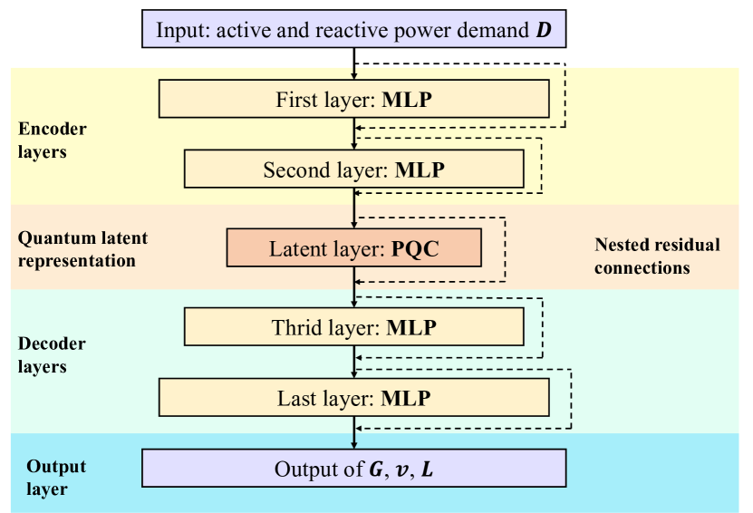
Figure 1: Flowchart of the sequential residual connection.

III-B2 Nested residual connection

The ”nested” residual connections indicate the residual connection from the encoder to its corresponding ”mirror” layer in the decoder. This kind of connection implies an assumption that these mirror layers encode or decode the same level of features in the NN. The implementation is presented in Fig.2. Assuming the PQC as the latent layer Q, the encoder layer l, and its mirror decoder layer L. With the residual identity connection, it can be presented as

$$y_{L}=x_{l}+f_{L}(x_{L},W_{L})$$ (12)

Let $x_{l}$ and $y_{l}$ denote the input and output of the $l$-th layer, respectively, while x and y represent the input and output of the $L$-th layer. The parameters $W_{l}$ and $W_{L}$ correspond to the weights and biases of the $l$-th and $L$-th layers. The function $f_{L}(\textperiodcentered)$ includes the layer operations along with the activation function. Since the decoder layer follows the encoder and includes the latent layer, Equation (11) can be reformulated as Equation (13). Here, $(q_{L}(f_{L}(x_{l},W_{l}),W_{q})$ represents the composite function that maps the encoder input $x_{l}$ to the decoder output $x_{L}$, indicating a multi-layer transformation through the network.

$$y_{L}=x_{l}+f_{L}(q_{L}(f_{L}(x_{l},W_{l}),W_{q}),W_{L})$$ (13)

According to automatic differentiation principles [13], the general derivative of the loss function with respect to can be used to compute the gradients for the parameters of the preceding layer, as shown in Equation (14). For simplicity, activation functions and batch normalization are omitted in the equation but are incorporated in the actual implementation to enhance the network’s representational capacity and to mitigate the ”vanishing gradient” problem.

$$\frac{\partial L}{\partial\mathbf{x}_{l}}=\frac{\partial L}{\partial\mathbf{y}_{L}}\cdot\left(1+\frac{\partial}{\partial\mathbf{x}_{l}}\left(f_{L}\left(g_{L}\left(f_{l}(\mathbf{x}_{l},\mathbf{W}_{l})\right),\mathbf{W}_{L}\right)\right)\right).$$ (14)

The inclusion of the constant term “1” in the loss function facilitates direct propagation of information from the decoder layer back to the corresponding encoder layer. This direct connection ensures that the gradient does not diminish excessively during back-propagation. Additionally, the second term following the constant “1” is not always -1 to make the gradient as 0; if it were, it could potentially cancel out the gradient, hindering learning. By preventing this cancellation, we partially avoid gradient vanishing and the subsequent degradation of network performance. Implementing these shortcut connections not only improves gradient flow but also accelerates the training process due to the more efficient gradient propagation.

Moreover, incorporating residual learning structures allows the network to learn identity mappings more effectively, which is crucial for deep networks like QNNs dealing with complex tasks such as OPF. This approach helps in maintaining the integrity of the original input information throughout the layers, leading to better convergence and improved overall performance.

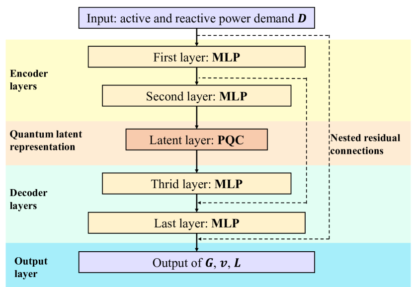
Figure 2: Flowchart of the nested residual connection.

III-C Physics-Informed Neural Networks

Physics-Informed Neural Networks (PINNs) are a class of neural networks trained to solve supervised learning tasks while adhering to physical laws described by nonlinear equations [14]. Specifically, PINNs integrate an additional physics layer after the typical neural network output to estimate the differential terms of the output variables. This integration allows the discrepancies in these differential terms—representing the ”physical loss”—to be incorporated into the neural network’s training loss function, calculated using the error between the estimated and actual differential variables. Consequently, the neural network’s output solution is validated against the loss associated with the physical constraints.

In the context of the AC-OPF problem, the PINN architecture aims to predict the active and reactive power generation set-points $G$, with the active and reactive power demands $D$ serving as inputs. Since the optimal solution must satisfy the KKT conditions specified in equations (4) to (8), the discrepancies in the KKT conditions—as shown in equations (15a) to (15d)—represent the physical loss and assisted training in (16).

$$\epsilon_{\text{stat}}=\left|c-\sum\hat{\lambda_{l}}a_{l}\right|+\left|\left(\sum\hat{\lambda_{l}}L_{l}+\sum\hat{\mu_{m}}M_{m}\right)\right|$$ (15-a)

$$\epsilon_{\text{comp}}=\sum\left|\hat{\mu_{m}}\left(\hat{v}^{T}M_{m}\hat{v}-d_{m}^{T}D-f_{m}\right)\right|$$ (15-b)

$$\epsilon_{\text{dual}}=\pi(\hat{\mu_{m}})$$ (15-c)

$$\epsilon_{\text{prim}}=\sum\left|\hat{v}^{T}L_{l}\hat{v}-a_{l}^{T}G-b_{l}^{T}D\right|$$ (15-d)

By combining the mean absolute errors (MAEs) for $G$, $v$ and $L$, as well the discrepancy in KKT conditions, the weighted faction of KKT loss and the NN loss in (17) is used to update the whole NN.

$$\begin{array}[]{lrl}L_{kkt}=\frac{1}{N_{t}+N_{c}}\sum_{i=1}^{N_{t}+N_{c}}\underbrace{\epsilon_{\text{stat}}+\epsilon_{\text{comp}}+\epsilon_{\text{dual}}+\epsilon_{\text{prim}}}_{MAE_{\epsilon}}\end{array}$$ (16)

$$\begin{array}[]{lrl}L_{kkt}=L_{nn}+\Lambda_{\epsilon}L_{kkt}\end{array}$$ (17)

A significant challenge in training PINNs is the sharp fluctuations that occur during the minimization of the equation loss and boundary-condition losses. Discrepancies in the KKT conditions can lead to suboptimal training performance. To enhance the efficiency of PINNs, various methods—including ensemble learning [15], point-weighting (PW) methods, and others—have been proposed to expedite the minimization process when dealing with competing error terms. However, since this paper focuses on integrating QNN techniques into PINNs, the weighting parameters in our proposed model are selected arbitrarily.

Furthermore, collocation points are incorporated into the training set to train the PINN layer by leveraging the KKT conditions to assess the accuracy of the neural network’s predictions. Specifically, collocation points are a set of random input values from the input domain, akin to the NN training data points. However, only the error terms specified in equations (11) are utilized to measure prediction accuracy and train the NN; the optimal generation dispatch values, voltage set-points, and dual variables are not computed for the collocation points prior to training, and their corresponding errors are set to zero. This technique has been validated to enhance the training efficiency of PINNs [5]. Notably, unlike approaches that employ three independent NNs to compute $G$, $v$, and $L$ separately, our PINN model utilizes a single NN to estimate all three types of variables. This unified approach facilitates a more straightforward implementation of QNN techniques, as discussed in the next section.

While PINNs have demonstrated significant potential in modeling real-world physical phenomena, they are not without limitations. One major challenge is the computational bottleneck encountered in high-dimensional problems, where the number of collocation points required to enforce physical laws increases exponentially, leading to prohibitively high computational costs [14]. Additionally, achieving convergence to acceptable levels of accuracy can be difficult [16]. The presence of multiple loss functions associated with partial differential equations (PDEs) and boundary conditions can result in competing objectives during training [17]. Furthermore, PINNs are susceptible to spectral bias—a tendency of neural networks to favor low-frequency functions—which can lead to trivial or suboptimal solutions [18]. The optimization of rugged loss landscapes in more complex problems is another significant failure mode for PINNs [19], further compounded by the issue of unbalanced back-propagated gradients during training [20].

IV Numerical results

To demonstrate the effectiveness of the proposed method, various case studies have been carried out on the IEEE standard test systems.

IV-A Simulation setup

The proposed method is tested against a standard NN and PINN on several different test systems. The detail of network for case 14 is from [21]. Moreover, the active and reactive power demand are assumed to be independent of each other.

Ten thousand sets of random active and reactive power input values were generated using latin hypercube sampling [22]. From these, $50\%$ were allocated to the collocation data set, for which we do not have to provide OPF set-points. $20\%$ of the rest was considered training data points and $30\%$ are served as test data set. AC-OPF in MATPOWER is used to determine the optimal active and reactive power generation values and voltage setpoints for the input data points in the training and test sets.

We used Pytorch [23] with Python for classic neural network training and Qiskit [24] for implementation and training process of PQC. The number of training epochs is fixed to be 2,000 and the data set is split into 50 batches while training.

V Conclusion

This paper developed two enhanced hybrid QNN architectures incorporating residual learning, which facilitated accelerated training processes and improved generalization performance. The residual connections effectively mitigated issues related to vanishing or exploding gradients, allowing for deeper network architectures without compromising convergence. Additionally, the integration of physics-informed layers embedded fundamental physical laws directly into the learning process. This ensured that the network’s predictions adhered to essential operational constraints like line capacities and bus voltage limits, thereby enhancing the reliability and feasibility of the solutions.

Simulation results demonstrated that the proposed hybrid QNNs significantly outperform conventional neural networks in solving OPF problems, even when trained on small or noisy datasets. The classical components, refined through residual learning and physics-informed techniques, are validated to be beneficial in optimizing performance and ensuring compliance with physical laws by simulation comparison. Potential directions include exploring optimization algorithms for alternative quantum circuit training and extending the approach to larger and more complex power systems.

References

- [1] M. B. Cain, R. P. O’neill, A. Castillo et al., “History of optimal power flow and formulations,” Federal Energy Regulatory Commission, vol. 1, pp. 1–36, 2012.
- [2] D. Bienstock and A. Verma, “Strong np-hardness of ac power flows feasibility,” Operations Research Letters, vol. 47, no. 6, pp. 494–501, 2019.
- [3] P. Kundur, “Power system stability,” Power system stability and control, vol. 10, pp. 7–1, 2007.
- [4] L. Duchesne, E. Karangelos, and L. Wehenkel, “Recent developments in machine learning for energy systems reliability management,” Proceedings of the IEEE, vol. 108, no. 9, pp. 1656–1676, 2020.
- [5] R. Nellikkath and S. Chatzivasileiadis, “Physics-informed neural networks for ac optimal power flow,” Electric Power Systems Research, vol. 212, p. 108412, 2022.
- [6] M. Schuld, I. Sinayskiy, and F. Petruccione, “The quest for a quantum neural network,” Quantum Information Processing, vol. 13, pp. 2567–2586, 2014.
- [7] K. Beer, D. Bondarenko, T. Farrelly, T. J. Osborne, R. Salzmann, D. Scheiermann, and R. Wolf, “Training deep quantum neural networks,” Nature communications, vol. 11, no. 1, p. 808, 2020.
- [8] Z. Kaseb, M. Möller, G. T. Balducci, P. Palensky, and P. P. Vergara, “Quantum neural networks for power flow analysis,” Electric Power Systems Research, vol. 235, p. 110677, 2024.
- [9] A. Narayanan and T. Menneer, “Quantum artificial neural network architectures and components,” Information Sciences, vol. 128, no. 3-4, pp. 231–255, 2000.
- [10] N. Killoran, T. R. Bromley, J. M. Arrazola, M. Schuld, N. Quesada, and S. Lloyd, “Continuous-variable quantum neural networks,” Physical Review Research, vol. 1, no. 3, p. 033063, 2019.
- [11] K. He, X. Zhang, S. Ren, and J. Sun, “Deep residual learning for image recognition,” in Proceedings of the IEEE conference on computer vision and pattern recognition, 2016, pp. 770–778.
- [12] L. Li, Y. Fang, J. Wu, J. Wang, and Y. Ge, “Encoder–decoder full residual deep networks for robust regression and spatiotemporal estimation,” IEEE transactions on neural networks and learning systems, vol. 32, no. 9, pp. 4217–4230, 2020.
- [13] A. G. Baydin, B. A. Pearlmutter, A. A. Radul, and J. M. Siskind, “Automatic differentiation in machine learning: a survey,” Journal of machine learning research, vol. 18, no. 153, pp. 1–43, 2018.
- [14] M. Raissi, P. Perdikaris, and G. E. Karniadakis, “Physics-informed neural networks: A deep learning framework for solving forward and inverse problems involving nonlinear partial differential equations,” Journal of Computational physics, vol. 378, pp. 686–707, 2019.
- [15] R. Polikar, “Ensemble learning,” Ensemble machine learning: Methods and applications, pp. 1–34, 2012.
- [16] S. Das and S. Tesfamariam, “State-of-the-art review of design of experiments for physics-informed deep learning,” arXiv preprint arXiv:2202.06416, 2022.
- [17] G. E. Karniadakis, I. G. Kevrekidis, L. Lu, P. Perdikaris, S. Wang, and L. Yang, “Physics-informed machine learning,” Nature Reviews Physics, vol. 3, no. 6, pp. 422–440, 2021.
- [18] N. Rahaman, A. Baratin, D. Arpit, F. Draxler, M. Lin, F. Hamprecht, Y. Bengio, and A. Courville, “On the spectral bias of neural networks,” in International conference on machine learning. PMLR, 2019, pp. 5301–5310.
- [19] A. Krishnapriyan, A. Gholami, S. Zhe, R. Kirby, and M. W. Mahoney, “Characterizing possible failure modes in physics-informed neural networks,” Advances in neural information processing systems, vol. 34, pp. 26 548–26 560, 2021.
- [20] S. Wang, Y. Teng, and P. Perdikaris, “Understanding and mitigating gradient flow pathologies in physics-informed neural networks,” SIAM Journal on Scientific Computing, vol. 43, no. 5, pp. A3055–A3081, 2021.
- [21] S. S. Khonde, S. Dhamse, and A. Thosar, “Power quality enhancement of standard ieee 14 bus system using unified power flow controller,” Int J Eng Sci Innov Technol, vol. 3, no. 5, 2014.
- [22] M. D. McKay, R. J. Beckman, and W. J. Conover, “A comparison of three methods for selecting values of input variables in the analysis of output from a computer code,” Technometrics, vol. 42, no. 1, pp. 55–61, 2000.
- [23] A. Paszke, S. Gross, F. Massa, A. Lerer, J. Bradbury, G. Chanan, T. Killeen, Z. Lin, N. Gimelshein, L. Antiga et al., “Pytorch: An imperative style, high-performance deep learning library,” Advances in neural information processing systems, vol. 32, 2019.
- [24] A. Javadi-Abhari, M. Treinish, K. Krsulich, C. J. Wood, J. Lishman, J. Gacon, S. Martiel, P. D. Nation, L. S. Bishop, A. W. Cross, B. R. Johnson, and J. M. Gambetta, “Quantum computing with Qiskit,” 2024.