Machine Learning Based Glitch Veto for inspiral binary merger signals using Linear Chirp Transform

Abstract

Unphysical templates for binary inspiral merger signals have emerged as an effective approach to veto signals ( rule out false signals ) identified as glitches. They offer a promising solution to reduce the number of parameters necessary for distinguishing glitches from actual gravitational wave merger signals. Glitches are short, transient noise artifacts that can mimic the characteristics of real signals, posing a significant challenge to gravitational wave detection. In this study, we investigate the application of the chirp transform — a modification of the traditional Fourier transform that incorporates an additional linear chirp axis, denoted by the chirp rate $\gamma$. This allows us to track signals with frequency changes over time more effectively, which is essential for gravitational wave analysis, particularly for inspiral and merger events. By applying the chirp transform to gravitational wave strain time series, we convert the signals into 3D spectrograms, with time, frequency, and chirp axes, thereby providing a richer dataset for signal analysis. These 3D representations capture more nuanced signal features, making them ideal for classification tasks. To enhance classification accuracy, we leverage convolutional neural networks ( CNNs ) trained on these spectrograms. CNNs are well-suited for image-based data like spectrograms of the signals. In our study, the networks have been optimized to differentiate between the spectrograms of glitch and merger signals. Our approach achieves high degree of accuracy on both the training and validation datasets, demonstrating the efficacy of combining the chirp transform with deep learning techniques for signal classification. Our method holds significant potential for improving glitch vetoes in gravitational wave detection, offering a more refined and computationally efficient classification process. The combination of advanced signal processing and machine learning paves the way for more reliable detection pipelines, ultimately enhancing the accuracy of observation from gravitational wave observatories like LIGO, VIRGO and upcoming detectors.

1 Introduction

Gravitational waves have become a critical area of research for validating Einstein’s theory of General Relativity, with Laser Interferometer Gravitational-Wave Observatory ( LIGO ) and VIRGO ( European Gravitational-Wave Observatory ) confirming the first direct detection in 2015 [1, 2]. With additions of other detectors like the Japanese gravitational wave KAGRA also known as Large-Scale Cryogenic Wave Telescope; upcoming additions like LIGO India; the advent of third-generation gravitational wave detectors like Einstein Telescope, Cosmic Explorer; upcoming Laser Interferometer Space Antenna ( LISA ) and other upcoming projects like Taiji, TianQin and Deci-Hertz Interferometer Gravitational Observatory ( DECIGO ) [3, 4, 5, 6, 7, 8, 9, 10] would expand our current knowledge on gravitational waves and their sources with more precise detections. These waves are ripples in the fabric of spacetime, produced when massive objects like binary black holes or neutron stars [11, 12] experience strong gravitational interactions and move rapidly. The most common sources of detectable gravitational waves are binary systems of black holes or neutron stars, which emit signals as they spiral toward each other and eventually merge—referred to as inspiral-merger signals [13].

The detection of the gravitational wave merger signals are in general done by templated or non-templated searches [14, 15]. Non-templated searches are based on the detection of a sudden chirp or increase in frequency similar to the simulated waveforms of binary merger signals. Templated search, as the name suggests, is searching via the correlation of a given signal to existing modelled templates. For templated search, the most widely used and accurate search is matched filtering [16]. Here we have a catalog of templates of waveforms that are simulated by changing the mass, distance from the detector’s line of sight, spin, etc, of the binary merger system but mainly the masses $(m_{1},\;m_{2})$ in order to get an accurate template. A given signal is matched with this template by correlation, and if it matches beyond a threshold, it is considered a candidate event, after which it has to be checked to see if it is a genuine merger signal. This has been the most reliable technique so far for detecting an inspiral binary merger waveform from a given signal.

Since the first detection, however, researchers have encountered signals that mimic these merger events, known as glitches [17]. These detectors are very sensitive and detect signals and monitor changes in length down to $10^{-19}\;\text{m}/\sqrt{\text{Hz}}$ variations [18] which is comparable to dimensions of the size of small atoms hence our detectors have to be very precise and sensitive. The presence of glitches that are much higher in noise and such transient artifacts mimicking the merger signals reduce the sensitivity of detectors significantly. Glitches are caused by various factors, such as environmental disturbances, instrumental noise, or even cosmic rays, and can obscure or imitate genuine gravitational wave signals. This presents a significant challenge for data analysis, as glitches must be accurately identified and filtered out to avoid misinterpreting noise as real astrophysical events. We want to eradicate every possible situation of false alarms to have the most accurate signal detection possible. Therefore every candidate event must go through a vetoing technique, where the glitches are ruled out and classified away from actual binary merger signals. We are taking into account those glitches that do bypass the matched filtering stage due to their close resemblance to the merger waveforms.

The paper will be organized as follows: In Section 2, we will discuss briefly the existing glitch veto methods and their limitations. Continuing in Section 3, we will introduce the JCTFT technique briefly and explain why we choose chirp transform for our inspiral signals. Next, in Section 4 - we will discuss data preparation and processing, followed by an exploration of the neural network architecture used for classification in Section 5 and the application of Principal Component Analysis ( PCA ) to the spectrogram distributions in Section 6. Finally, we will present our conclusions in Section 7.

2 Existing Glitch-veto methods

2.1 Traditional Chi-Square Veto

Initially, the Chi-square method [19] was used to distinguish glitches from real signals by comparing the orthogonal projections of a signal in a parameter space. The Chi-square ( $\chi^{2}$ ) method is a statistical technique that measures how well an observed data set matches an expected model or distribution. In the context of glitch detection in gravitational wave signals, the Chi-square method involves calculating the discrepancies between the observed signal and a theoretical template across different segments of the signal. For each segment, the signal is projected onto an orthogonal parameter space defined by the physical characteristics of the system, such as frequency, phase, or amplitude. By comparing these projections to the expected values based on models of merger signals, the Chi-square statistic can quantify how closely the signal aligns with a real gravitational wave event. The sum of squared differences between the observed and expected projections across all segments is computed to yield the Chi-square value. If the signal significantly deviates from the model in some regions, as is often the case with glitches, the Chi-square value increases, flagging the signal as anomalous. Conversely, a low Chi-square value suggests the signal closely matches the expected pattern, making it more likely to be a genuine gravitational wave event. However, the challenge with this approach lies in the diversity of glitches. Since there are around 22 distinct classes of glitches [20] with different characteristics, the parameter space for each glitch type needs to be carefully tailored, making the method computationally expensive. Moreover, the Chi-square method is not foolproof — glitches with certain characteristics that can still slip through the veto mechanism, lead to false positives in the detection process.

Despite these limitations, the core idea remains foundational in many veto techniques: finding a parameter space where the behavior of glitches and merger signals diverges, allowing for their separation.

2.2 Recent Glitch-veto techniques: Unphysical templates

In response to the limitations of traditional glitch classification techniques, researchers have explored more efficient methods, such as the use of unphysical waveform templates to distinguish glitches from real gravitational wave signals [21]. Initially, this approach focused on the masses of the binary components in a system, assuming that certain mass combinations would correspond to physically plausible signals while others would not. By comparing the mass estimates derived from observed signals with these pre-defined mass regions, researchers hoped to identify glitches. However, this method was found to be somewhat ineffective due to the fact that the physical and unphysical regions of the mass parameter space do not have clearly defined boundaries. The overlap between the two regions means that distinguishing between a glitch and a real signal based purely on mass estimates was often ambiguous, leading to both false positives and false negatives. As a result, researchers recognized the need for more sophisticated parameters that could better separate physically realistic signals from glitches by defining a parameter space with sharper delineations. In the work [21], new parameters called the chirp time parameters ( $\tau_{0}$ and $\tau_{1}$ ) have been introduced. These parameters describe the evolution of the signal’s frequency over time in the context of the 2PN ( second post-Newtonian ) waveform. Specifically, $\tau_{0}$ and $\tau_{1}$ define the rate at which the waveform’s frequency changes with time for the zeroth and first orders of frequency, respectively. These chirp time parameters are closely related to the component masses of the binary system, such that the physical and unphysical mass regions can be translated into the chirp time parameter space. Similar work was also done using chirp masses which are defined a bit differently but correlates mass and the chirp rates analytically [22]. By using these chirp time parameters, we avoid directly assigning binary component masses, $m_{1}$ and $m_{2}$, to the waveform template. Instead, we assign $\tau_{0}$ and $\tau_{1}$ values to the template, which provides a more nuanced and effective method for distinguishing between real gravitational wave signals and glitches. This shift to chirp time parameters allows for a more accurate classification of signals and glitches, as the unphysical regions in the $\tau_{0}$ and $\tau_{1}$ space correspond more clearly to glitch-like behavior, while the physical regions align with real merger events. The template search is done here by Particle Swarm Optimization(PSO) [23] which is a stochastic algorithm and proves faster given that we take the correct initial guess at the start. The advantages of this approach are numerous. For instance, this new veto technique [21], which is based on the chirp time parameters, achieves an impressive accuracy of approximately 99.9 percent. By leveraging the unphysical regions of the chirp time parameter space, this technique is able to veto about 70 percent of glitches, significantly reducing the number of false positives. In addition, the technique makes use of the differences in Signal-to-Noise Ratios ( SNRs ) and the Time of Arrival ( TOA ) of the signals to enhance the veto process further. These additional comparisons provide a robust framework for identifying glitch signals that may not be easily separable by chirp time parameters alone. Despite its success, there are still challenges with this vetoing technique. One major issue lies in the use of Particle Swarm Optimization ( PSO ) for matching templates to observed signals. PSO is a powerful optimization method, but it works best in search spaces that are hypercubical in shape. Unfortunately, the regions defined in the $\tau_{0}$ and $\tau_{1}$ parameter space are not hypercubical, which means that the PSO search is not fully optimized for this application. As a result, there are cases where the technique may not find the best possible match between the signal and the template, reducing its overall efficiency. Additionally, this method may miss higher-mass binary systems and a few signals, as the chirp time parameters are primarily based on the 2 Post Newtonian ( 2PN ) approximation [24], which is not always a perfect representation of the actual gravitational waveforms from such systems. The 2PN approximation is an analytical solution that describes the inspiral phase of a binary merger and not an exact solution for a given binary merger signal. As such, the parameter space defined by $\tau_{0}$ and $\tau_{1}$ may not capture all possible signal variations, especially for extreme systems. Furthermore, this vetoing technique still relies to some extent on noise profiling, as the parameter regions are inherently influenced by the noise characteristics of the detector. Although the use of chirp time parameters and unphysical regions provides a more reliable way to distinguish between real signals and glitches, the presence of noise in the detector can still affect the performance of the method. This latest vetoing technique is 99.9 percent accurate but has challenges.

Various other methods have also been developed with the help of machine learning such as General Adversial Networks ( GANs ), Similarity learning and Characterization of detectors, etc [25, 26, 27]. All these let very few glitches bypass their veto; hence we need to be using more than one vetoing technique. Search for one particular vetoing technique is sought so that the pipeline for signal processing is made lighter computationally and we make sure we have all the glitches vetoed and have no false alarm signals.

Our work takes a slightly unconventional approach. We utilize the Joint Chirp Rate Fourier Transform (JCTFT) to analyze the correlations within the spectrograms derived from these signals in the chirp axis. This method allows us to explore differences between glitch and merger signals, aiming to reduce the parameter space required for glitch classification. We further use neural networks on the 3 dimensional spectrograms we get from JCTFT to classify. Instead of using a parameter space and using one constant parameter per given signal, we look at the change in the spectrograms at the Linear Chirp parameter space for classification. Our study will aim to provide a working model that will classify glitches from merger signals for candidate events that have passed the matched filtering stage and aid other existing techniques in vetoing the transient glitches.

3 Joint Chirp Rate Time Frequency Transform ( JCTFT )

In previous research [28], the Joint Chirp Rate Time Frequency Transform ( JCTFT ) technique was introduced as a novel method for analyzing gravitational wave signals. The JCTFT extends the conventional Fourier transform by incorporating a linear chirp rate, denoted by $\gamma$, which represents the rate of change of frequency over time ( with units of $T^{-2}$ ). Specifically, a linear chirp signal’s frequency can be modeled as $f(t)=f_{0}+\gamma t$, where the frequency changes linearly with time at the rate $\gamma$. This allows the JCTFT to capture the time-frequency behavior of signals that exhibit frequency evolution, which is typical for many astrophysical processes, including inspiral-merger signals.

The importance of the chirp rate in gravitational wave signals, particularly those from inspiral - merger events, cannot be overstated. Such signals evolve in frequency as compact objects spiral toward each other before merging, resulting in a rapidly increasing frequency near the merger. In essence, the JCTFT correlates the signal not only with frequency but also with the chirp rate by introducing a $\gamma t^{2}$ term in the phase of the transform. This addition enables the detection of signals with varying frequencies by accounting for the rate at which the frequency changes. While the frequency model of inspiral-merger signals is complex and typically nonlinear, a linear chirp serves as a first approximation for improving the response to these signals.

Thus, with the JCTFT, we obtain a 3D spectrogram (time, frequency, and chirp rate $\gamma$) instead of a traditional 2D time-frequency spectrogram. This added dimension provides richer information, potentially revealing subtle features in the signal that may be lost in a purely time-frequency analysis. Figure 1 illustrates the 3D spectrogram we get for a given signal. Mathematically, the JCTFT can be expressed as an extension of the standard Fourier transform:

$$H(\Omega)=\int_{-\infty}^{\infty}h(t)e^{-i2\pi\Omega t},dt$$ (1)

Equation (1) represents the traditional Fourier transform [29, 30], where the signal $h(t)$ is correlated with a phase function of frequency $\Omega$. This gives insight into the power distribution in the frequency domain. However, this approach is limited when dealing with signals whose frequency evolves over time. To address this, the JCTFT introduces a chirp term:

$$H(\Omega,\gamma)=\int_{-\infty}^{\infty}h(t)e^{-i2\pi(\Omega t+\gamma t^{2})},dt$$ (2)

Equation (2) represents the Linear Chirp Transform ( LCT ), a generalization of the Fourier transform that introduces the $\gamma t^{2}$ term in the phase. This additional term accounts for the linearly increasing frequency ( i.e., the chirp ) at the rate $\gamma$. When differentiating the phase, it becomes evident that the frequency of the signal increases linearly over time, making the JCTFT highly suitable for signals like gravitational waves, where the frequency evolution is a key feature.

In the process of applying the JCTFT to a signal $h(t)$, discretization [31] becomes crucial for practical analysis. The discretized JCTFT can be represented as a convolution between the Fourier transform of $h(t)$ and the Fourier transform of the window function that incorporates the chirp $\gamma t^{2}$ term. Specifically, for the product of two functions in the time domain, the convolution theorem allows us to take the convolution of the Fourier transforms of the individual functions shown in Equations 3 and 4. We choose a Gaussian window function for this convolution, although other window functions can be selected for different purposes, such as to enhance time or frequency resolution.

$$H(\gamma,\tau,\Omega)=\mathcal{F}\{f(t)g_{c}(t-\tau,\gamma,\Omega)\}=\mathcal{F}\{f(t)\}\ast\mathcal{F}\{g_{c}(t-\tau,\gamma,\Omega)\}$$ (3)

$$=\mathcal{F}\{f(t)\}\ast\mathcal{F}\{g_{c}(t,\gamma,\Omega)\}e^{-i2\pi\Omega\tau}$$ (4)

In equation 5, $g_{c}$ represents the Gaussian window function, and $\tau$ denotes the time shift.
The window function $g_{c}$ is defined as follows:

$$g_{c}(\gamma,t-\tau,\Omega)=\frac{\left|\Omega_{0}+\mu\Omega\right|}{\sqrt{2\pi\left(1+\frac{t-\tau}{|t-\tau|^{2}}\right)}}e^{-(t-\tau)^{2}\left(\frac{(\Omega_{0}+\mu\Omega)^{2}}{2}+i2\pi\gamma\right)}$$ (5)

This window function [32] is key to extracting meaningful frequency and chirp rate information from a given segment of the signal. A detailed analysis of different window functions and their impact on chirp transform performance can be found in [28]. In our work, we opt for the Gaussian window due to its well-known properties in time-frequency analysis, balancing the trade-off between time and frequency localization. Especially for signals with chirp, it smoothens out local regions of the signal, effectively preventing any spectral leakage. The window function adjusts well according to the frequency and chirp variations locally.

Here, $g_{c}$ incorporates the chirp term and normalization factors, ensuring that the window function is appropriately scaled. This function resembles sliding functions used in time-frequency analysis techniques like the S-Transform [33]. A significant advantage of the JCTFT lies in its ability to provide a more sensitive response to signals with chirping behavior compared to traditional Fourier-based techniques, which are less effective in capturing non-stationary features.

The Fourier transform of the window function $g_{c}$ has an exact solution, derived as follows:

$$G_{c}(\gamma,\Omega,\alpha)=\frac{|\Omega_{0}+\mu\Omega|}{\sqrt{2\pi}}\left(e^{-\pi^{2}\alpha^{2}/z}\left(\frac{\sqrt{\pi}}{2\sqrt{z}}\left(1-\operatorname{erf}\left(\frac{i\pi\alpha}{\sqrt{z}}\right)\right)\right)\right)$$ (6)

In this expression, $G_{c}(\gamma,\Omega,\alpha)$ represents the Fourier transform of the window function, without any time shift, where $\alpha$ is the shift in frequency. The availability of an exact solution simplifies the process of computing the JCTFT, as the Fourier transform of the signal $h(t)$ can be convolved with this pre-computed solution, thereby enabling efficient computation. It is possible to have higher chirp terms ( say $t^{3},t^{4}...$ and even fractional chirp term $t^{-7/6}$, etc. ) in such a way that it exactly matches the order of our inspiral merger signal’s waveforms but they would not have an exact solution and give us a nice discretized version like the Linear Chirp transform. There is a huge possibility of inferences that could open up if we could derive the analytical solutions of the same. But for now in [28], it was demonstrated that gravitational wave signals from inspiral-merger events, which exhibit an increasing frequency as the objects approach each other, are well-suited for analysis using the JCTFT. This is because the positive chirp of these signals naturally aligns with the chirp dimension in the JCTFT, enhancing signal detection even in low signal-to-noise ratio ( SNR ) conditions. Empirical tests with SNRs as low as 5, up to 15, consistently showed that the JCTFT provided better performance in detecting these signals than the Q-Transform for signals with lower SNRs

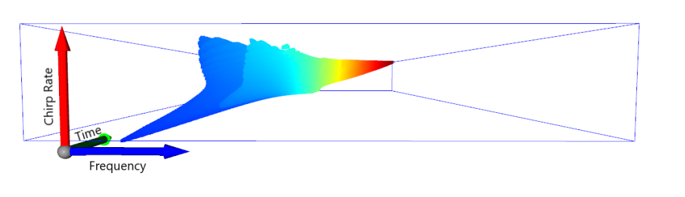
Figure 1: 3D spectrogram output of a clean merger signal strain visualized. X. Li, M. Houde, and S. Valluri et., al. [28]
Notation: The Time axis is in the direction into the page

To validate the effectiveness of the JCTFT, a comparative study was conducted using the Inception V3 network [34, 35] for signal classification. Signals were analyzed using both the JCTFT and the Q-Transform [36], and it was found that for signals with low SNRs, the JCTFT significantly outperformed the Q-Transform, particularly in the detection of weak signals where the chirp behavior is critical. Figure 2 illustrates the classification results between the two methods.

In our present work, we now aim to leverage the same JCTFT technique for our glitch classification pipeline, building upon the proven effectiveness of the JCTFT in gravitational wave signal detection. By utilizing the richer information provided by the 3D time-frequency-chirp spectrograms, we expect to improve the performance of glitch classification, especially for signals with complex frequency evolution.

Figure 2: Comparison of Detection accuracy by InceptionV3 Network on JCTFT v/s Q-Transform. X. Li, M. Houde, and S. Valluri et.,al. [28]

4 Data

Below we will discuss the strain data used from LIGO’s Hanford and Livingston Detectors. We have trained a huge catalogue of data- both glitches and merger signals. The nature of the data and preprocessing are discussed below in the upcoming sub-sections.
The goal would be to process data to the finest detail and reduce it to minimum memory to save the computational cost and time. After the chirp transform we want the data in a format which is very light for the model to train on since it will be working with 1000s of signals and has to be integrated with a live working pipeline later on.

4.1 Glitches

The glitches used in this study were provided by R. Girgaonkar and S. D. Mohanty et.,al. [21], who identified them in their research. These glitches consist of 708 individual instances of time series strain data, which include attributes such as Time of Arrival ( TOA ), Signal-to-Noise Ratio ( SNR ), and other relevant parameters like Xspacing, starting and ending time, etc. The data were sourced from LIGO’s and VIRGO’s open-access databases, specifically from the Gravitational Wave Open Science Center ( GWOSC ) [37]. After downloading the data, it was further processed to estimate the Time of Arrival ( TOA ) and the chirp rates $\tau_{0}$ and $\tau_{1}$ for each signal ( not to be confused with our linear chirp rate $\gamma$ ). In their work, these chirp rates were used to generate templates that delineated physical and unphysical regions in the signal analysis.

For consistency with our simulated merger signals, which are also 6 seconds in duration, we have clipped each glitch signal to a 6-second window centered around its TOA. This duration was chosen because it aligns with the typical length of transient glitches, which generally last for only a few seconds. Additionally, this choice helps manage computational costs, as longer signals would result in significantly larger chirp transform outputs, making the analysis more resource-intensive. While we have set this 6-second window as our current standard, future improvements in machine learning models may allow us to reduce this duration even further, potentially enabling the classification of shorter signal segments.

The dataset encompasses a range of SNR values, from a minimum of 9 to a maximum of 14401, and includes glitches recorded during both LIGO Livingston and LIGO Hanford runs. This variety ensures a comprehensive representation of glitch characteristics across different SNR levels and observational settings.

4.2 Merger Signals

They are simulated signals used in previous work [28] to compare the performance of Inception V3 network to detect signals from JCTFT spectrograms versus Q-Transform spectrograms. It is based on a simplified Binary Black hole ( BBH ) instantaneous frequency(IF) model given by [38] which when followed by a 2PN correction in time domain is described by Equation (7) given below:

$$\text{IFmerger}(t)=\frac{5^{3/8}}{8\pi}\left(\frac{c^{3}}{GM_{\text{chirp}}}\right)^{\frac{5}{8}}(t_{c}-t)^{-\frac{3}{8}}$$ (7)

where G is gravitational constant, $t_{c}$ is the coalesence time, and $M_{\text{chirp}}$ is chirp mass defined by the individual masses $m_{1}$ and $m_{2}$ of the binary system defined in Equation(8):

$$M_{\text{chirp}}=\frac{(m_{1}m_{2})^{\frac{3}{5}}}{(m_{1}+m_{2})^{\frac{1}{5}}},\quad m_{1}>0,\,m_{2}>0$$ (8)

We use PyCBC’s SEOBNRv4 model [39] for simulating the above waveforms and varying parameters. The distance along the line of sight of the detector is varied from 600 Mpc -1200 Mpc and the signals having different time of arrivals. The distances are 600 Mpc, 800 Mpc, 1000 Mpc, 1200 Mpc with 3 different time of arrivals- i.e the peak signal arrival in either 1st, 2nd or 3rd part of the 6 second signal. We add varying random noise ( gaussian ) that mimic the noise in usual merger signals detected. For each variation of the parameters we have 72 signals.
Hence we have in total 72* 4 ( distance variation ) * 3 ( signal arrival variation ) = 864 merger signals. These are simulated by varying the masses of the binary system, distance, etc.
$m_{1}$, $m_{2}$ are varied between 5 and 41.6 $M_{\odot}$ where $M_{\odot}$ equals 1 Solar mass. The Peak Signal-Noise Ratio ( PSNR ) ranges from 4.19-86.88 while the Blurred Signal-Noise Ratio ( BSNR ) ranges from 3 to 5 for these simulated signals.
These are the very signals used in the work of JCTFT [28] for the purpose of testing the Linear Chirp transform technique on signals of varying SNRs. We use these in order to make sure that our model has comparatively equal number of signals for both glitches and merger signals to ensure we don’t overfit our model in bias towards one class ( glitch or merger signals )

4.3 Chirp transform and preprocessing

To effectively manage and analyze the extensive arrays produced by our chirp transform, we have implemented a strategy that balances data efficiency with analytical precision.

For each 6-second signal processed through the chirp transform, we generate a large array with dimensions of ( 61, 471, 6000 ). Here, the dimension 61 corresponds to the chirp axis, which ranges from -30 to 30 with a step size of 1. The dimension 471 represents the frequency range, spanning from 30 Hz to 500 Hz. The reason we pick this frequency range is because 30 Hz is the lower cutoff of what the detector could acquire and though the upper cutoff for the detector is 700Hz most of the physically possible inspiral merger signals fall within the 500 Hz range ( with exception of some very high mass binaries ). To keep computational cost at a reasonable level we stop with 500 Hz cutoff since our model which we later design is adept even for this frequency range input. Finally, the dimension 6000 corresponds to the time samples, which are derived based on a Nyquist sampling rate of 1000 [40] to accommodate the 500 Hz cutoff ( minimum downsampling rate= 2 * frequency cutoff. In our case 2 * 500 = 1000 ). This results in a complex datatype array that occupies approximately 1.2 GB of storage.

Handling such voluminous datasets for thousands of signals presents considerable challenges in terms of both storage and processing capacity. To address these challenges, we have devised a method to reduce the size and complexity of the data while retaining its analytical value.

Instead of retaining the complete complex arrays, we have opted to compute and store the absolute power distributions derived from these arrays. Specifically, we extract slices from each of the 61 two-dimensional time-frequency spectrograms, dividing them into positive and negative chirp domains ( with 30 slices in each domain ). For each slice, we generate a histogram with 100 bins, representing the normalized power distribution. Normalization is performed such that the peak power for each slice is scaled to 1, and the total sum of the counts in the histogram is also normalized to 1.

This approach effectively compresses the data by converting it into a more manageable format. The normalized histograms are saved as CSV ( comma separated values ) files, designated as $positive\_X.csv$ and $negative\_X.csv$, where $X$ represents a unique identifier for each signal. This transformation reduces the file size of each CSV to approximately 964 kB, which significantly lowers the total storage requirement per signal to under 2 MB. This preprocessing is explained in Figure 3.

By focusing on these normalized power distributions, we achieve two major benefits: we alleviate storage constraints and streamline data processing and analysis. This method not only facilitates the handling of thousands of signals more efficiently but also simplifies the interpretation of the data. With the data now compact and well-organized, we can turn our attention to optimizing the architecture of our classification network to achieve robust performance in signal classification.

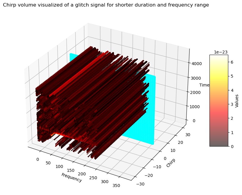
(a) 3D chirp volume spectrogram for a glitch signal -sample slice at chirp-rate = 0

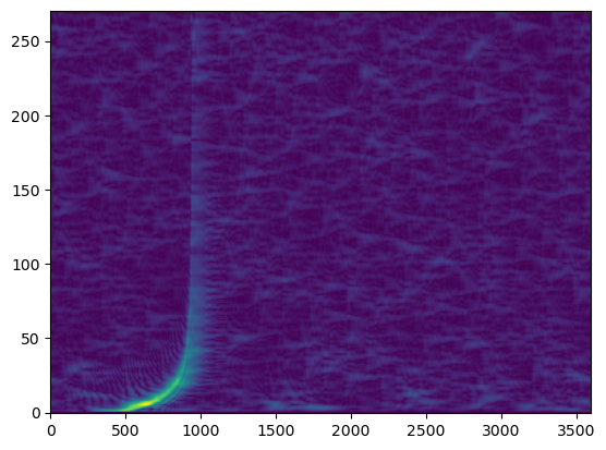
(b) 2D time-frequency spectrogram at chirp-rate = 0

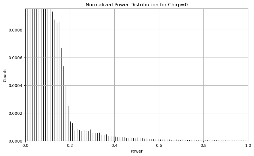
(c) Normalized power distribution for a given chirp-rate slice

Figure 3: The chirp transform and preprocessing: (a), (b), and (c) correspond to the positive and negative domain distributions saved in CSV files: positive.csv and negative.csv for all slices in the range [-30, 30].

5 Network model

We deploy Convolutional Neural Networks ( CNNs ) for this classification task [41] due to their ability to effectively analyze histogram distributions and capture subtle variations across different chirp indices. CNNs are widely used in image processing due to their proficiency in reducing dimensionality and detecting spatial patterns. In our case, CNNs are well-suited for distinguishing between glitches and mergers because they can detect minute differences in the power distributions despite the presence of noise. The input to our model consists of the CSV files, $positive\_X.csv$ and $negative\_X.csv$, which contain the normalized histogram distributions of each signal. These distributions are processed through the CNN to classify the signal as either a glitch or a merger.

Figure 4: Network architecture used for the model. X here is a unique identifier for a given signal

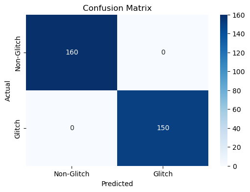
Figure 5: Validation performance on test dataset - testsize $\approx$ 0.2 of the total dataset or 310 signal samples

The architecture of our CNN model ( given in Figure 4 ) is designed to efficiently process and analyze the histogram data. Initially, the normalized data distributions from both the positive and negative chirp domains are fed into a 1D convolutional layer. This layer utilizes 32 filters with a kernel size of 3, and employs the Rectified Linear Unit ( ReLU ) activation function [42]. The ReLU function introduces non-linearity into the model, allowing it to learn more complex patterns in the data. The kernel size [43] is chosen small ( = 3) so that the 3*3 matrix slides over our 1D - like chirp histogram data ( at every slice index ) and captures the smallest features possible. A larger kernel size could be taken for the convolutional operation but we don’t want to lose out on the intricate features since glitches and merger signals are closely mimicking each other and it is the smallest of changes we want to capture to classify.

Following the convolutional layer, we apply Max Pooling [44] to down-sample the data and reduce its dimensionality, which helps to highlight the most prominent features while mitigating overfitting. We also incorporate dropout with a rate of 0.25 to prevent the model from relying too heavily on any specific neurons, thus improving its generalization capabilities.

The next stage of the network includes another convolutional layer with 64 filters with the same kernel size=3 and ReLU activational function. This deeper layer enhances the model’s capacity to identify more intricate features in the data by increasing the number of filters and maintaining the ReLU activation function. Again, Max Pooling is applied to further reduce the dimensionality and focus on the most relevant features.

After these convolutional and pooling operations, the resulting feature maps are flattened into a one-dimensional vector. This flattened vector is then passed through a dense layer, where another dropout rate of 0.5 is employed. The dense layer enables the network to combine and interpret the learned features from previous layers, while the dropout helps to prevent overfitting by eliminating less significant features.

The final output layer is a softmax regression node [45], which provides probabilities for the signal being a glitch or a merger. The softmax function transforms the network’s output into a probability distribution over the two classes, allowing us to make a classification decision based on which class’ probability exceeds 0.5.

We train the model for 20 epochs, and it achieves 100 percent accuracy on both the training and validation sets within a few epochs. This remarkable performance suggests that the model is effectively learning the distinguishing features of glitches. We considered the possibility that this high accuracy could be due to noise profiling, given that glitches are real data with inherent noise while merger signals are simulated. However, the model maintains 100 percent accuracy even when random noises, similar to real noise, are injected into the merger signals, and high SNR glitch signals are adjusted ( such that overall SNR ranges randomly from 1-10 ). Note that this robustness is confirmed since we have not re-trained the model based on these new injections and test it with the model previously trained on our initial simulated merger and glitch signal catalogue available. This robustness indicates that the model is not simply memorizing noise patterns but is genuinely distinguishing between glitches and merger based on their intrinsic characteristics.

To further validate our approach, we perform Principal Component Analysis (PCA) [46] on the signals to explore how well they separate in a reduced-dimensional space. This analysis helps confirm whether the model’s high accuracy reflects meaningful distinctions between signal types.

Overall, the choice of CNNs is justified by their ability to effectively process the histogram data, capture intricate patterns, and manage the data’s high dimensionality. By combining convolutional layers with pooling, dropout, and dense layers, our model is well-equipped to handle the complexities of the signal classification task and achieve high performance.

In Figure 5 we plot the confusion matrix[47] that shows how well the model is predicting against the true label ( glitch or merger signal ) for a random test size of 0.2 or 20 percent of the whole dataset available.

6 Principal Component Analysis ( PCA )

In this study, we utilized Principal Component Analysis ( PCA ) to reduce the dimensionality of the features extracted from the normalized histogram distributions representing the signals. Our primary aim was to visualize the differences between glitch and merger signals in a lower-dimensional space, which would make patterns more discernible and facilitate a better understanding of the underlying structure in our data.
PCA is a statistical technique that transforms high-dimensional data into a set of orthogonal axes known as principal components, capturing the directions of maximum variance. By projecting our high-dimensional feature space onto two principal components, we could create a 2D representation that highlights the most significant patterns and differences within the dataset. Specifically, we computed PCA1 and PCA2. PCA1 corresponds to the direction of maximum variance and represents the first principal component derived from a linear combination of various histogram bins from both the positive and negative chirp domains. Similarly, PCA2 captures the second most significant variance, providing additional context and further distinguishing features that are orthogonal to PCA1.

The visualization of the signals along these principal components, as illustrated in Figure 6, revealed a notable separation between glitch and merger signals. Most signals were clearly clustered into distinct groups, corresponding to either glitches or mergers, with some instances of overlap. This clear separation indicates that the statistical characteristics of glitches and mergers are sufficiently distinct to be differentiated based on their principal components. The PCA analysis effectively highlighted these differences, supporting the robustness of our preprocessing steps.

However, despite the clear separation, some overlap between the two signal types remained. This overlap can be attributed to the inherent variability within the signals and potential limitations in the feature extraction process. To address these challenges and achieve more accurate classification, we employed Convolutional Neural Networks ( CNNs ). CNNs are particularly adept at learning complex patterns and relationships within the data, providing a higher level of accuracy than PCA alone. While PCA serves as a valuable tool for initial exploration and visualization, advanced models like CNNs are essential for achieving superior classification performance. [48]

The precise linear combinations that define PCA1 and PCA2 are detailed in the supplementary materials available on our GitHub repository. The scripts contains an exhaustive list of contributing factors and weights used to compute the principal components which is not possible to give as an equation in the context of this paper. But as explained earlier they are linear combinations of the bins data from both positive and negative chirp distributions such that the power distribution ( or counts of bins here ) have the most variance possible.

In summary, PCA proved to be an effective method for dimensionality reduction and visualization, revealing distinct patterns that differentiate glitch and merger signals. While PCA provided valuable insights into the data, the application of CNNs further enhanced our classification accuracy, demonstrating the complementary role of these techniques in our analysis.

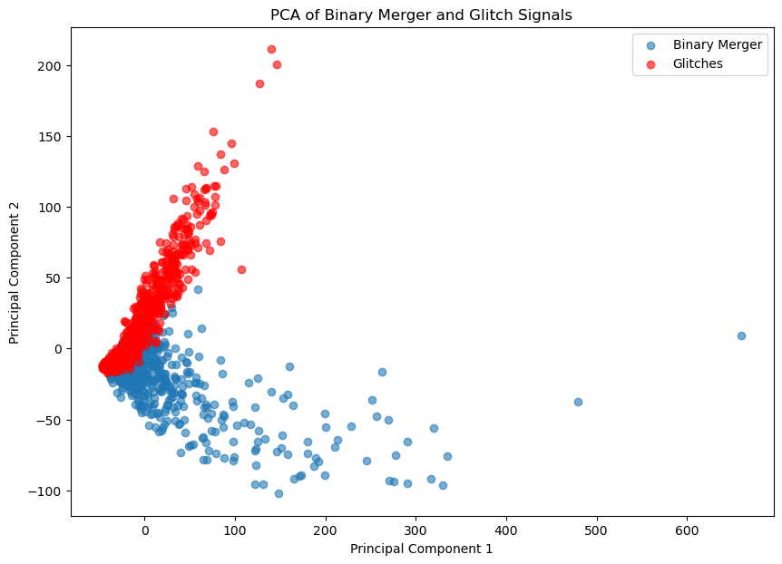
Figure 6: Principal Component Analysis ( PCA ) of the normalized distributions. PCA1 represents the linear combination of histogram bins that captures the most variance while PCA2 captures the second most variance in the power distribution. The plot shows a clear separation between glitches and mergers, with some overlap indicating the need for advanced classification techniques. These principal components help visualize the differences between signal types and support the robustness of our classification approach.

7 Conclusion and future possibilities

We have presented a machine learning-based method of the chirp transform to classify glitches from merger signals. Our approach is intended to be a part of the LIGO pipeline after a signal has passed the matched filtering stage and is labelled as a candidate event. We ran the model on a single core of the AMD Ryzen 5 - 4600H 6-core CPU. It took around 32.7 seconds to perform the chirp transform, process, and store the desired CSV files. The stored trained model takes 30 ms to classify if a given signal is a glitch or not, when we input the positive and negative chirp domain distributions.
This gives a highly accurate model for classification of glitches in the context of inspiral merger signals. Though trained for LIGO detectors, the logic of signals separating out in the chirp domain could be used for new age and advanced future detectors. As new types of glitches are discovered they could be included in the model. Further analysis could be done to infer more about the applications of the chirp transform for signal processing. More could be inferred from deriving the transform for higher chirp rates or fractional chirp rates.
Getting an exact solution is a daunting task but estimates for specific signal processing purposes could be made. One could get well fitted analytical solutions; thereby the inference one could get from various signals could be better leveraged. The Chirp transform has already shown its usefulness in other domains like Radio Detection and Ranging ( RADAR ) and other signal processing tasks [49, 50]. Improvement on solutions of other polynomial chirp rates would contribute to domains that have specific waveform models.
Furthermore it is possible to have better data storage methods for the heavy 3D spectrograms so that one could gain more information about a given signal. When this pipeline is included with the best computing resources available - one would get a quicker performance since the model is fast on conventional computers with minimum resources as well.
To summarise, we have a highly accurate pipeline to classify glitches from genuine inspiral merger signals. We intend to study other types of glitches like gamma-ray pulsars, fast radio bursts, etc and test our methodology for gravitational wave detection.

8 Acknowledgement

This work was undertaken under MITACs Globalink GRI’24 fellowship. We acknowledge valuable suggestions given by Dr. Soumya Mohanty and Raghav Girgaonkar of University of Texas Rio Grande Valley who gave a vision and kickstart to this work by their recent research, sharing the data and suggesting an application of the chirp transform. We also acknowledge Dr.Martin Houde of Western University,Ontario in playing a key role while developing the Chirp Transform. We thank the authors of Tensorflow, Numpy, Matplotlib, PyCBC, GWPy, Scipy and Pandas which we used to complete our work,model and visualise in a rapid manner [39, 51, 52, 53, 54, 55, 56, 57].

Data Availability - All the scripts and data used could be found in our github repository- https://github.com/Arut123/Glitch-veto-GW-using-chirp

References

- [1] Benjamin P Abbott et al. “GW150914: The Advanced LIGO detectors in the era of first discoveries” In Physical review letters 116.13 APS, 2016, pp. 131103
- [2] Benjamin P Abbott et al. “Observation of gravitational waves from a binary black hole merger” In Physical review letters 116.6 APS, 2016, pp. 061102
- [3] “KAGRA: 2.5 generation interferometric gravitational wave detector” In Nature Astronomy 3.1 Nature Publishing Group UK London, 2019, pp. 35–40
- [4] M Saleem et al. “The science case for LIGO-India” In Classical and Quantum Gravity 39.2 IOP Publishing, 2021, pp. 025004
- [5] Karsten Danzmann and Albrecht Rüdiger “LISA technology—concept, status, prospects” In Classical and Quantum Gravity 20.10 IOP Publishing, 2003, pp. S1
- [6] M Punturo et al. “The Einstein Telescope: A third-generation gravitational wave observatory” In Classical and Quantum Gravity 27.19 IOP Publishing, 2010, pp. 194002
- [7] Wen-Rui Hu and Yue-Liang Wu “The Taiji Program in Space for gravitational wave physics and the nature of gravity” In National Science Review 4.5 Oxford University Press, 2017, pp. 685–686
- [8] Soichiro Isoyama, Hiroyuki Nakano and Takashi Nakamura “Multiband Gravitational-Wave Astronomy: Observing binary inspirals with a decihertz detector, B-DECIGO” In Progress of Theoretical and Experimental Physics 2018.7 Oxford University Press, 2018, pp. 073E01
- [9] David Reitze et al. “Cosmic explorer: the US contribution to gravitational-wave astronomy beyond LIGO” In arXiv preprint arXiv:1907.04833, 2019
- [10] Jun Luo et al. “TianQin: a space-borne gravitational wave detector” In Classical and Quantum Gravity 33.3 IOP Publishing, 2016, pp. 035010
- [11] Francois Foucart “A brief overview of black hole-neutron star mergers” In Frontiers in Astronomy and Space Sciences 7 Frontiers Media SA, 2020, pp. 46
- [12] Tejaswi Venumadhav et al. “New search pipeline for compact binary mergers: Results for binary black holes in the first observing run of Advanced LIGO” In Physical Review D 100.2 APS, 2019, pp. 023011
- [13] Abhirup Ghosh et al. “Testing general relativity using gravitational wave signals from the inspiral, merger and ringdown of binary black holes” In Classical and Quantum Gravity 35.1 IOP Publishing, 2017, pp. 014002
- [14] Tanmaya Mishra et al. “Search for binary black hole mergers in the third observing run of Advanced LIGO-Virgo using coherent WaveBurst enhanced with machine learning” In Physical Review D 105.8 APS, 2022, pp. 083018
- [15] Tejaswi Venumadhav et al. “New search pipeline for compact binary mergers: Results for binary black holes in the first observing run of Advanced LIGO” In Physical Review D 100.2 APS, 2019, pp. 023011
- [16] Benjamin J Owen and Bangalore Suryanarayana Sathyaprakash “Matched filtering of gravitational waves from inspiraling compact binaries: Computational cost and template placement” In Physical Review D 60.2 APS, 1999, pp. 022002
- [17] S Mukherjee, R Obaid and B Matkarimov “Classification of glitch waveforms in gravitational wave detector characterization” In Journal of Physics: Conference Series 243.1, 2010, pp. 012006 IOP Publishing
- [18] Robert E Colgan et al. “Efficient gravitational-wave glitch identification from environmental data through machine learning” In Physical Review D 101.10 APS, 2020, pp. 102003
- [19] Sanjeev Dhurandhar, Anuradha Gupta, Bhooshan Gadre and Sukanta Bose “A unified approach to 2 discriminators for searches of gravitational waves from compact binary coalescences” In Physical Review D 96.10 APS, 2017, pp. 103018
- [20] Daniel George, Hongyu Shen and EA Huerta “Classification and unsupervised clustering of LIGO data with Deep Transfer Learning” In Physical Review D 97.10 APS, 2018, pp. 101501
- [21] Raghav Girgaonkar and Soumya D Mohanty “Glitch veto based on unphysical gravitational wave binary inspiral templates” In Physical Review D 110.2 APS, 2024, pp. 023037
- [22] Nirban Bose, Archana Pai, Koustav Chandra and V Gayathri “Chirp mass based glitch identification in long-duration gravitational-wave detection” In Physical Review D 102.8 APS, 2020, pp. 084034
- [23] James Kennedy and Russell Eberhart “Particle swarm optimization” In Proceedings of ICNN’95-international conference on neural networks 4, 1995, pp. 1942–1948 ieee
- [24] Eric Poisson and Clifford M Will “Gravitational waves from inspiraling compact binaries: Parameter estimation using second-post-Newtonian waveforms” In Physical Review D 52.2 APS, 1995, pp. 848
- [25] Jade Powell et al. “Generating transient noise artefacts in gravitational-wave detector data with generative adversarial networks” In Classical and Quantum Gravity 40.3 IOP Publishing, 2023, pp. 035006
- [26] Siddharth Soni et al. “Discovering features in gravitational-wave data through detector characterization, citizen science and machine learning” In Classical and Quantum Gravity 38.19 IOP Publishing, 2021, pp. 195016
- [27] S Coughlin et al. “Classifying the unknown: discovering novel gravitational-wave detector glitches using similarity learning” In Physical Review D 99.8 APS, 2019, pp. 082002
- [28] Xiyuan Li, Martin Houde and SR Valluri “A Complex Window-Based Joint-Chirp-Rate-Time-Frequency Transform for BBH Merger Gravitational Wave Signal Detection” In arXiv preprint arXiv:2209.02673, 2022
- [29] Henri J Nussbaumer and Henri J Nussbaumer “The fast Fourier transform” Springer, 1982
- [30] Ronald N Bracewell “The fourier transform” In Scientific American 260.6 JSTOR, 1989, pp. 86–95
- [31] Osama A Alkishriwo and Luis F Chaparro “A discrete linear chirp transform (DLCT) for data compression” In 2012 11th International Conference on Information Science, Signal Processing and their Applications (ISSPA), 2012, pp. 1283–1288 IEEE
- [32] KM Muraleedhara Prabhu “Window functions and their applications in signal processing” Taylor & Francis, 2014
- [33] Robert Glenn Stockwell, Lalu Mansinha and RP Lowe “Localization of the complex spectrum: the S transform” In IEEE transactions on signal processing 44.4 IEEE, 1996, pp. 998–1001
- [34] Biswajit Jena, Gopal Krishna Nayak and Sanjay Saxena “Convolutional neural network and its pretrained models for image classification and object detection: A survey” In Concurrency and Computation: Practice and Experience 34.6 Wiley Online Library, 2022, pp. e6767
- [35] Rahul Suresh and N Keshava “A survey of popular image and text analysis techniques” In 2019 4th international conference on computational systems and information technology for sustainable solution (CSITSS), 2019, pp. 1–8 IEEE
- [36] Judith C Brown and Miller S Puckette “An efficient algorithm for the calculation of a constant Q transform” In The Journal of the Acoustical Society of America 92.5 Acoustical Society of America, 1992, pp. 2698–2701
- [37] LIGO Scientific Collaboration and Virgo Collaboration “Open Data from the First and Second Observing Runs of Advanced LIGO and Advanced Virgo”, 2021
- [38] LIGO Scientific et al. “The basic physics of the binary black hole merger GW150914” In Annalen der Physik 529.1-2 Wiley Online Library, 2017, pp. 1600209
- [39] Christopher Michael Biwer et al. “PyCBC Inference: A Python-based parameter estimation toolkit for compact binary coalescence signals” In Publications of the Astronomical Society of the Pacific 131.996 IOP Publishing, 2019, pp. 024503
- [40] HJ Landau “Sampling, data transmission, and the Nyquist rate” In Proceedings of the IEEE 55.10 IEEE, 1967, pp. 1701–1706
- [41] Zewen Li et al. “A survey of convolutional neural networks: analysis, applications, and prospects” In IEEE transactions on neural networks and learning systems 33.12 IEEE, 2021, pp. 6999–7019
- [42] Raman Arora, Amitabh Basu, Poorya Mianjy and Anirbit Mukherjee “Understanding deep neural networks with rectified linear units” In arXiv preprint arXiv:1611.01491, 2016
- [43] Zhun Sun, Mete Ozay and Takayuki Okatani “Design of kernels in convolutional neural networks for image classification” In Computer Vision–ECCV 2016: 14th European Conference, Amsterdam, The Netherlands, October 11–14, 2016, Proceedings, Part VII 14, 2016, pp. 51–66 Springer
- [44] Haibing Wu and Xiaodong Gu “Max-pooling dropout for regularization of convolutional neural networks” In Neural Information Processing: 22nd International Conference, ICONIP 2015, Istanbul, Turkey, November 9-12, 2015, Proceedings, Part I 22, 2015, pp. 46–54 Springer
- [45] Zihao Yuan et al. “Softmax regression design for stochastic computing based deep convolutional neural networks” In Proceedings of the on Great Lakes Symposium on VLSI 2017, 2017, pp. 467–470
- [46] Hervé Abdi and Lynne J Williams “Principal component analysis” In Wiley interdisciplinary reviews: computational statistics 2.4 Wiley Online Library, 2010, pp. 433–459
- [47] Jingsai Liang “Confusion matrix: Machine learning” In POGIL Activity Clearinghouse 3.4, 2022
- [48] Abhilash Kayyidavazhiyil and Mario Silic “INTRUSION DETECTION USING DEEP (CNN) CONVOLUTIONAL NEURAL NETWORK FEATURE EXTRACTION WITH (EPCA) ENHANCED PRINCIPAL COMPONENT ANALYSIS FOR DIMENSIONALITY REDUCTION” In Global journal of Business and Integral Security, 2022
- [49] Mio Horai, Hideo Kobayashi and Takashi G Nitta “Chirp signal transform and its properties” In Journal of Applied Mathematics 2014.1 Wiley Online Library, 2014, pp. 161989
- [50] Mark Roberton and ER Brown “Integrated radar and communications based on chirped spread-spectrum techniques” In IEEE MTT-S International Microwave Symposium Digest, 2003 1, 2003, pp. 611–614 IEEE
- [51] Charles R Harris et al. “Array programming with NumPy” In Nature 585.7825 Nature Publishing Group UK London, 2020, pp. 357–362
- [52] Bo Pang, Erik Nijkamp and Ying Nian Wu “Deep learning with tensorflow: A review” In Journal of Educational and Behavioral Statistics 45.2 SAGE Publications Sage CA: Los Angeles, CA, 2020, pp. 227–248
- [53] Wes McKinney “pandas: a foundational Python library for data analysis and statistics” In Python for high performance and scientific computing 14.9 Seattle, 2011, pp. 1–9
- [54] Pauli Virtanen et al. “SciPy 1.0: fundamental algorithms for scientific computing in Python” In Nature methods 17.3 Nature Publishing Group, 2020, pp. 261–272
- [55] Duncan M Macleod et al. “GWpy: A Python package for gravitational-wave astrophysics” In SoftwareX 13 Elsevier, 2021, pp. 100657
- [56] Ekaba Bisong and Ekaba Bisong “Matplotlib and seaborn” In Building machine learning and deep learning models on google cloud platform: A comprehensive guide for beginners Springer, 2019, pp. 151–165
- [57] Qian-Yi Zhou, Jaesik Park and Vladlen Koltun “Open3D: A modern library for 3D data processing” In arXiv preprint arXiv:1801.09847, 2018