Learning Approximated Maximal Safe Sets via Hypernetworks for MPC-Based Local Motion Planning

Abstract

This paper presents a novel learning-based approach for online estimation of maximal safe sets for local motion planning tasks in mobile robotics. We leverage the idea of hypernetworks to achieve good generalization properties and real-time performance simultaneously. As the source of supervision, we employ the Hamilton-Jacobi (HJ) reachability analysis, allowing us to consider general nonlinear dynamics and arbitrary constraints. We integrate our model into a model predictive control (MPC) local planner as a safety constraint and compare the performance with relevant baselines in realistic 3D simulations for different environments and robot dynamics. The results show the advantages of our approach in terms of a significantly higher success rate: 2 to 18 percent over the best baseline, while achieving real-time performance.

I INTRODUCTION

Safety persists as one of the key challenges in the field of autonomous robotics. Real-world applications require modern robots to be performant in naturally unstructured and uncertain enironments. At the same time, they are expected to maintain rigorous safety standards during operation, especially in environments shared with humans. Achieving required performance and safety simultaneously motivated development of many advanced optimization-based [1, 2, 3], sampling-based [4, 5], and learning-based [6, 7] algorithms for local motion planning. Also, hybrid architectures [8, 9] and safety filters [10, 11] exhibit solid potential in fulfilling the two objectives.

Local motion planning becomes especially difficult when the robot’s actuation is significantly limited or when the task imposes additional restrictions on robot movements [12]. Actuation capabilities are usually limited by design, while applications such as mobile manipulation or transportation of heavy and unstable objects require very smooth motion of the mobile base. All those restrictions, combined with other safety constraints such as collision avoidance, can drastically reduce the set of allowed operating states of a robot, which we refer to in this paper as the safe set.

Our work focuses on estimating the maximal safe sets for obstacle avoidance tasks in cluttered environments. Our aim is to efficiently integrate the resulting safe set representation with a model predictive control (MPC) local planner. We first numerically calculate the true maximal safe regions via the Hamilton-Jacobi (HJ) reachability framework for a set of binary costmaps based on particular robot dynamics. Then, we use the resulting dataset to train a model architecture consisting of a hypernetwork and the main network in a supervised fashion. The hypernetwork learns how to parameterize the main network for different binary costmaps while the main network renders the corresponding estimated maximal safe set in real-time, which we use as a safety constraint within the MPC planner.

Compared to existing approaches based on HJ reachability, our method can approximate the HJ value function in real time for continually changing high-dimensional local observations in unknown environments. We illustrate this with a nonholonomic mobile robot navigating based on the stream of local costmaps. To the best of our knowledge, none of the existing methods can be applied to such a scenario without additional simplifying assumptions. Therefore, the approach introduced in this paper brings a great improvement in applicability of HJ reachability for time-critical systems. The main contributions of this paper are the following:

• A novel learning-based approach for real-time estimation of maximal safe sets for nonlinear systems based on local observations of an unknown environment, which is not achieved by the existing methods.

• A novel hybrid architecture integrating learned maximal safe sets as constraints with an MPC local planner achieving real-time performance.

II RELATED WORK

One of the core problems in local motion planning is designing environment representation based on sensor data and integrating it within the planner in real time. The representation has to provide sufficient information to safely avoid obstacles while progressing along the reference path. In practice, a signed distance field (SDF) calculated based on Euclidian distance [13, 14, 15] is a common choice. This representation is intuitive [16] and can be efficiently generated even in 3D space [17]. Also, recent works employ different ML techniques to learn a neural SDF and then use it for robot perception and motion planning [18, 19, 20].

The primary disadvantage of an SDF is the failure to account for the robot dynamics and actuation limits. The safe set associated with an SDF is usually an overapproximation of the maximal safe set, leading to higher collision rates. One possible alternative is to use control barrier functions (CBFs) [21, 22], which are successfully applied for local motion planning in different scenarios [23]. There is also related work on time-varying cases [24], vision-based control [25], and integration of CBFs as safety constraints with MPC local planners [26, 27, 28].

Even though CBFs can provide desirable safety guarantees, designing a proper CBF for a general nonlinear dynamical system remains very challenging. There is certain progress on systems with control limits [29, 30, 31] and systems with state constraints [32]. Many authors propose different learning-based methods for CBF design [33, 34, 35]. Nevertheless, CBFs designed in those approaches usually fail to characterize the maximal safe regions well, resulting in either conservative or unsafe motion.

Computing the true maximal safe regions is possible with HJ reachability analysis, which is a numerical framework for model-based computation of reachable sets [29, 32, 36, 37]. This framework suffers from the curse of dimensionality and is impractical for high-dimensional and time-critical systems. To overcome this issue, authors in [38] use an ML model to reduce the associated computational complexity, while authors in [39] use a neural network model to approximate the solution of HJ reachability. However, those approaches assume complete a priori knowledge about the environment, which is not satisfied for most real-world systems. In that regard, the work in [40] introduces parameter-conditioned reachable sets by augmenting system dynamics with a set of virtual states representing environment-dependant parameters. This idea is applied for motion planning tasks in mobile robotics [41] and autonomous driving [42]. The main limitation is that the method can only handle up to 3 environmental parameters. In contrast, our approach conditions maximal safe sets based on a local costmap consisting of 101$\times$101 cells (10201 environment parameters), improving the existing approaches by four orders of magnitude without increasing the dimensionality of the original system as in [40].

Compared with other methods for safe navigation in unknown environments, the main advantage of our approach is improved real-time performance. For example, the method in [43] also uses the HJ value function as the safety constraint, but it requires $\sim$600 ms to find a solution in the best case. A different approach is presented in [44] where safety constraints are initially extracted from demonstrations and the belief over those constraints is updated online based on observations, which takes minimally 1.4 s per update. In contrast, depending on the horizon length and robot model, our method takes 10-50 ms on average for trajectory optimization as presented in Section V. Additionally, our method does not include any hand-coded components such as feature functions that are used in [45].

III PRELIMINARIES

III-A Problem Formulation

We consider a nonlinear dynamical system

$$\dot{x}(t)=f(x(t),u(t)),$$ (1)

where $x(t)\in\mathbb{R}^{n}$ represents system’s state vector, $u(t)\in\mathbb{R}^{m}$ is the control vector, and $t\in\mathbb{R}$ denotes the time variable. The discrete-time form of Eq. 1 is

$$x_{k+1}=f_{d}(x_{k},u_{k}),$$ (2)

where $k\in\mathbb{Z}$ is the discrete-time variable, $x_{k}$ and $u_{k}$ are state and control vectors at time $t=k\cdot\delta t$ for a fixed sampling time $\delta t$, and $f_{d}$ is discrete-time model obtained by some discretization method from the continuous-time dynamics $f$.

Since our aim is to employ an MPC local planner, we first define the corresponding optimal control problem that is solved iteratively at every time step $k$:

$$\min_{u_{k:k+N-1}}\quad p(x_{k+N})+\sum_{i=0}^{N-1}q(x_{k+i},u_{k+i})$$ (3a)

$$s.t.\quad x_{k+i+1}=f_{d}(x_{k+i},u_{k+i}),\,i=0:N-1$$ (3b)

$$x_{k+i}\in\mathcal{X},\quad i=0:N$$ (3c)

$$u_{k+i}\in\mathcal{U},\quad i=0:N-1$$ (3d)

$$h_{k}(x_{k+i})\geq 0,\quad i=0:N$$ (3e)

In this formulation, $x_{k+i}$ and $u_{k+i}$ are predictions of the state and control vectors at future time $k+i$ made at the current time step $k$ over the horizon of length $N$. Equality constraint Eq. 3b enforces the optimal solution to satisfy the system’s dynamics, Eq. 3c and Eq. 3d constrain predicted state and control vectors to have admissible values, while Eq. 3e is an inequality constraint that incorporates any additional requirements imposed on the system states. The cost terms $p$ and $q$ depend on a specific task and in this paper we use the standard quadratic form:

$$q(x,u)=(x-x_{r})^{\top}Q(x-x_{r})+u^{\top}Ru,$$ (4)

$$p(x)=(x-x_{r})^{\top}Q_{N}(x-x_{r}),$$ (5)

where $x_{r}$ is the reference state and $R$, $Q$ and $Q_{N}$ are weight matrices. We focus our attention on ${h:\mathbb{Z}\times\mathbb{R}^{n}\rightarrow\mathbb{R}}$ in Eq. 3e and the main problem addressed in this paper is how to design function $h$ in real time such that its zero-superlevel set approximates the maximal safe region.

III-B Hamilton-Jacobi Reachability

HJ reachability analysis is a verification method for dynamical systems used to guarantee the safety and performance properties of a system under state and input constraints and external disturbances. More formally, HJ reachability allows us to compute the backward reachable tube (BRT), which is a set of states such that if a system’s trajectory starts from this set, it will eventually end up inside some target set [37, 39]. In the context of local motion planning for mobile robots, one can think of a BRT as a region around obstacles from which collision will happen inevitably at some point in time (e.g., due to long braking distance or limited steering).

Even though HJ reachability generally considers disturbed or uncertain nonlinear dynamical systems [37], in this work we consider only deterministic systems described by Eq. 1. If we assume that the system starts at state $x(t)$, then we denote with $\xi^{u}_{x,t}(\tau)$ the system’s state at time $\tau$ after applying $u(\cdot)$ over time horizon $[t,\tau]$. Here, we assume that $f$ satisfies standard assumptions of the existence and uniqueness of the state trajectories. We denote the set of target states as $\mathcal{L}$ and define BRT for which the system will reach the target set $\mathcal{L}$ within the time horizon $[t,T]$ as

$$\mathcal{V}(t)=\{x:\forall u(\cdot),\,\exists\tau\in[t,T],\,\xi^{u}_{x,t}(\tau)\in\mathcal{L}\}.$$ (6)

In order to compute BRT for a given target set, we first define $\mathcal{L}$ as a zero-sublevel set of the target function $l(x)$, i.e. $\mathcal{L}=\{x:l(x)\leq 0\}$. After that, the computation of the BRT is formulated as an optimization problem that seeks to find the minimal distance to the set $\mathcal{L}$ over the time horizon

$$J(x,t,u(\cdot))=\min_{\tau\in[t,T]}l(\xi^{u}_{x,t}(\tau)).$$ (7)

In the case that $\mathcal{L}$ represents an unsafe region, the goal is to find the optimal control that will maximize this distance. Therefore, we introduce the value function corresponding to this optimal control problem:

$$V(x,t)=\sup_{u(\cdot)}\{J(x,t,u(\cdot))\}.$$ (8)

The value function is computed over a state-space grid using dynamic programming, resulting in the final value Hamilton-Jacobi-Isaacs Variational Inequality (HJI VI) [46, 47]:

$$\min\left\{\frac{\partial}{\partial t}V(x,t)+H(x,t),\,l(x)-V(x,t)\right\} =0,$$ (9)

$$V(x,T) =l(x).$$

In the formulation above, Hamiltonian $H(x,t)$ is defined as

$$H(x,t)=\max_{u}\nabla V(x,t)\cdot f(x,u).$$ (10)

Once the value function Eq. 8 is calculated, the corresponding BRT can be obtained as its zero-sublevel set, i.e.

$$\mathcal{V}(t)=\left\{x:V(x,t)\leq 0\right\},$$ (11)

and the maximal safe set is its complement.

IV METHODOLOGY

The main goal is to design the constraint in Eq. 3e online based on available local observations of the environment and provide it to the MPC planner. Calculating maximal safe regions for general nonlinear systems under control and state constraints involves solving Eq. 9, which is intractable in real time. Therefore, we aim for ML techniques capable of learning a mapping from environment observation to the approximation of the maximal safe set in the form of a parameterized model.

IV-A Model Architecture

The designed model has to satisfy two conflicting objectives: generalize well across a wide spectrum of possible observations and allow for computationally efficient trajectory optimization in real time. Adequate generalization requires expressive models, i.e., models with a large number of trainable parameters optimized on a vast amount of data. On the other side, a computationally efficient representation requires a simple model architecture with a relatively small number of parameters. This feature is particularly important for local planners that rely on iterative numerical optimization methods such as gradient-based optimization.

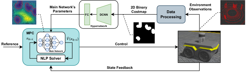
Figure 1: The proposed local motion planning architecture with neural value function as the safety constraint.

Our approach separates the ML model into two neural networks. The first network processes the local representation of the environment (e.g., local costmap) and outputs the parameters of the second network, which represents the constraint function in Eq. 3e. In the literature, the first network is referred to as hypernetwork, and the second network is known as main network [48, 49]. The hypernetwork is designed to be expressive and have many trainable parameters to achieve desired generalization properties. Complementary, the main network is a simple and efficient model that approximates the maximal safe set corresponding only to the current observation of the environment. During the motion planning, the hypernetwork is inferred only once per time step to parametrize the main network which is then provided to the optimization algorithm as a constraint function and it is iteratively queried for its value and gradient. As argued in [50], the overall number of trainable parameters can be orders of magnitude smaller compared to the embedding-based approach. Also, we perform experiments with a single-network architecture to justify benefits of the hypernetworks for real-time performance.

In our concrete implementation, we assume that the local observation is provided as a 2D binary costmap. This is a common representation used in practice for ground mobile robots and can be efficiently computed from sensor readings such as a LiDAR point cloud. Since the input is in the form of a single-channel image, our hypernetwork consists of a deep convolutional neural network (DCNN) backbone and a fully connected (FC) head. After the parameters are obtained, the main network is used as a safety constraint which approximates the value function in Eq. 8 and implicitly the maximal safe set. The only assumption is that the costmap is large enough so that the obstacle is visible before the robot enters the corresponding BRT. As a main network, we use a simple multi-layer perception (MLP) model. The overall architecture of our approach is presented in Fig. 1.

IV-B Training Procedure

The hypernetwork is trained in a supervised fashion and therefore we need both input data and ground truth labels. The input data in our implementation is a set of 2D binary costmaps and a set of state-space grid points for the concrete robot dynamics. We can obtain costmaps from a simulation environment or use a dataset recorded in real-world experiments, while the state-space grid points are generated by a uniform discretization of the state space depending on the desired resolution and individual state limits.

We utilize HJ reachability to calculate the true value function in Eq. 8 over the state-space grid for a theoretically infinite-time horizon and use those values as the labels for the predicted value function $\hat{V}(x)$ at the output of the main network. To calculate the true value function $V(x)$, the target function $l(x)$ is needed as the terminal constraint in Eq. 9. Since our target region represents occupied space in a costmap, we define $l(x)$ as the SDF calculated over the same costmap as indicated in the training diagram in Fig. 2.

Regarding the cost function, one can consider the mean squared error (MSE), which is a standard cost function in regression tasks. This cost function penalizes prediction errors equally over the whole state-space grid. However, the main purpose of the learned value function is to separate safe and unsafe regions by its zero-level set. Therefore, we propose the following weighted MSE (WMSE) cost function that favors higher prediction accuracy near the zero-level set of the true value function:

$$L =\frac{1}{M}\sum_{i=1}^{M}\frac{1}{K}\sum_{j=1}^{K}w_{i,j}(V_{i,j}-\hat{V}_{i,j})^{2},$$ (12)

$$w_{i,j} =1+\alpha\exp\left(-\beta V_{i,j}^{2}\right),\quad\alpha,\beta\in\mathbb{R}^{+}.$$

In the equations above, $M$ is the total number of training samples (costmaps), $K$ is the number of states in the state-space grid, while $\alpha$ and $\beta$ represent hyperparameters of the cost function. Qualitatively speaking, the value of $\alpha$ determines the relative weighting of the prediction error near the zero-level set, while the value of $\beta$ controls the width of the margin around the zero-level set that is weighted higher. The proposed WMSE empirically improves characterization of the maximal safe sets and results in enhanced safety. The complete training procedure is visualized in the Fig. 2.

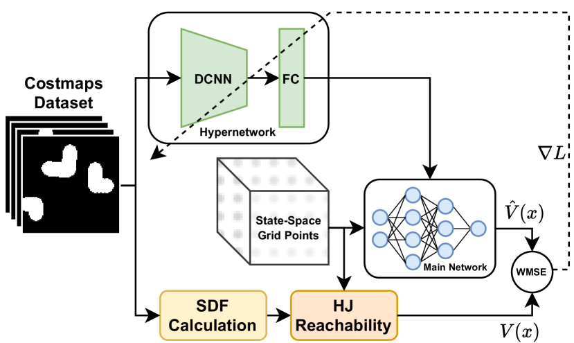
Figure 2: Training diagram for the proposed model architecture.

V EXPERIMENTAL RESULTS

V-A Robot Models

In this subsection we describe the two types of nonholonomic robot dynamics that we analyze in our experiments.

Model 1: The first model is the 2nd-order unicycle model, which is used in practice to model differential drive and skid-steer types of robots. The state vector of this model is ${x=[x_{p},\,y_{p},\,\theta,\,v,\,\omega]^{\top}}$, where $x_{p}$ and $y_{p}$ are positional coordinates, $\theta$ is orientation, while $v$ and $\omega$ are linear and angular velocities, respectively. The control vector ${u=[a,\,\alpha]^{\top}}$ consists of linear acceleration $a$ and angular acceleration $\alpha$, while the dynamics is defined as

$$\dot{x}=\left[v\cos(\theta),\,v\sin(\theta),\,\omega,\,a,\,\alpha\right]^{\top}.$$ (13)

For this model, we assume the following state and control constraints: ${v\in[-1,1]}$ m/s, ${\omega\in[-3,3]}$ rad/s, ${a\in[-1,1]}$ m/s², and ${\alpha\in[-3.55,3.55]}$ rad/s².

Model 2: The second model is the 1st-order unicycle model with positive minimal linear speed and asymmetric limits for angular speed. This model could be used to model plane-like mobile robots with a broken wing or a ground mobile robot with a damaged steering mechanism that cannot stop its motion completely. The state vector has three components ${x=[x_{p},\,y_{p},\,\theta]^{\top}}$ and control vector is ${u=[v,\omega]}$. Dynamics in this case is

$$\dot{x}=\left[v\cos(\theta),\,v\sin(\theta),\,\omega\right]^{\top},$$ (14)

and limits are: ${v\in[0.25,0.5]}$ m/s, ${\omega\in[-0.25,0.5]}$ rad/s.

V-B Monte Carlo Simulations

TABLE I: Quantitative results from the Monte Carlo simulations

Robot model $\rightarrow$		Model 1				Model 2
N	Method	Success rate [%]		Mean opt. time [ms]		Success rate [%]		Mean opt. time [ms]
		Env. 1	Env. 2	Env. 1	Env. 2	Env. 1	Env. 2	Env. 1	Env. 2
$15$	NVF-MPC	90	77	48.79 $\pm$ 3.41	49.40 $\pm$ 5.08	76	68	31.32 $\pm$ 5.25	28.75 $\pm$ 4.71
	DCBF-MPC	74	75	24.49 $\pm$ 3.86	26.90 $\pm$ 5.01	58	56	22.29 $\pm$ 5.30	18.24 $\pm$ 3.06
	DSDF-MPC	70	67	16.74 $\pm$ 2.76	16.58 $\pm$ 2.44	43	48	17.14 $\pm$ 4.38	13.26 $\pm$ 3.30
$10$	NVF-MPC	81	76	32.19 $\pm$ 3.07	34.14 $\pm$ 3.70	79	68	19.93 $\pm$ 3.26	19.71 $\pm$ 3.13
	DCBF-MPC	68	78	16.29 $\pm$ 2.78	17.70 $\pm$ 2.73	48	51	14.54 $\pm$ 3.02	13.48 $\pm$ 2.64
	DSDF-MPC	60	54	12.49 $\pm$ 2.29	12.35 $\pm$ 1.94	22	35	12.87 $\pm$ 2.62	10.27 $\pm$ 2.81
$5$	NVF-MPC	78	66	16.71 $\pm$ 0.72	17.56 $\pm$ 1.88	79	68	11.67 $\pm$ 1.04	10.65 $\pm$ 1.01
	DCBF-MPC	60	74	8.74 $\pm$ 0.71	10.28 $\pm$ 0.95	39	40	8.42 $\pm$ 1.06	8.54 $\pm$ 1.54
	DSDF-MPC	26	21	8.55 $\pm$ 1.35	8.63 $\pm$ 0.62	14	28	8.32 $\pm$ 1.15	7.21 $\pm$ 1.81

We perform Monte Carlo simulations for the two types of robot dynamics described above in two different environments using the Gazebo 3D simulator. The first environment (Env. 1) is a warehouse model and the second environment (Env. 2) is a house model. As the relevant baselines, we examine MPC local planners with two other representations of the safety constraint in Eq. 3e. The first baseline uses a discrete SDF as a collision avoidance constraint [16] and we refer to it as DSDF-MPC. The second baseline called DCBF-MPC uses a safety constraint as given in [26, Example A], which resembles a discrete-time CBF. This method defines the safety constraint as follows:

$$\Delta h_{SDF,k}(x_{k})\geq-\gamma h_{SDF,k}(x_{k}),$$ (15)

where $\Delta h_{SDF,k}(x_{k})=h_{SDF,k}(x_{k+1})-h_{SDF,k}(x_{k})$, $h_{SDF,k}$ is an SDF observed at time $k$ and $\gamma\in(0,1]$. Since our method uses the neural value function as the constraint for an MPC local planner, we refer to it as NVF-MPC. All the methods are implemented in the CasADi framework [51] using IPOPT solver and deployed as a ROS2 package on Intel mini PC. Sampling time for controllers is 0.1 s while the simulator runs in real time.

The task is to drive the robot from the initial position to the goal position, which we assume to be two successive waypoints provided by a global planner. The success rate is considered the primary metric that indicates local planning performance in a cluttered environment. The mean optimization time is also recorded as an indicator of real-time feasibility. We observe that other metrics such as the mean MPC cost value and the mean time to complete the task have approximately the same values for different methods, so we exclude them from the results.

We train two hypernetwork models implemented in PyTorch for the two robot dynamics on a set of 30K costmaps (5$\times$5 m with 101 cells along both dimensions) and the corresponding value functions. The costmaps used for training are recorded only in the warehouse environment, and the robot is tested in both environments to evaluate the generalization properties. The WMSE hyperparameters in Eq. 12 are set to $\alpha=1000$ and $\beta=100$ based on grid search. The hypernetwork architecture is the same for both robot models, while the main network is adapted to meet required complexity for individual models.

For both environments, we generate 100 scenarios with a random distribution of 3 to 4 obstacles between the start and goal positions in order to make the task challenging for the local planners. Then, we perform experiments with our approach and the baselines for 3 lengths of the MPC prediction horizon: 15, 10 and 5 time steps. The parameter $\gamma$ in Eq. 15 is set to 0.1 in all experiments. An experiment is considered a failure if a collision occurs or the robot does not reach its goal within a time limit. Video recordings of some of the experiments can be found in the supplementary material and the obtained quantitative results are presented in Table I.

Based on the results, we conclude that our approach outperforms the baselines in most of the experiments while still being real-time feasible. The only case when the DCBF-MPC performs slightly better is Model 1 dynamics in the house environment (Env. 2) for shorter horizons. The reason is the fact that our model was not trained on any data from this environment and generalization should be further improved, e.g., by recording a more comprehensive dataset from different environments. However, for Model 2 our method drastically improves the success rate even in the test environment (Env. 2) because the shapes of the maximal safe sets are very complex.

Experiments with fixed computational budget: In order to make a more comprehensive evaluation of the NVF-MPC method, we perform additional experiments with increased horizon lengths of the baselines. Since the average optimization time of our approach is larger for the given horizon lengths, we increase the baselines’ horizons so that all methods have a similar optimization time. We assume that the maximal allowed optimization time is equal to the average optimization time needed for NVF-MPC with the horizon length of 15 steps ($\sim$50 ms for Model 1 and $\sim$30 ms for Model 2). In the case of DSDF-MPC we managed to increase the horizon up to 25 or 30 steps and in the case of DCBF-MPC up to 20 or 25 steps. We performed experiments with 100 trials for all four combinations of robot dynamics and environment models. Based on the obtained results presented in Fig. 3, our approach outperforms the baselines for the given computational resources.

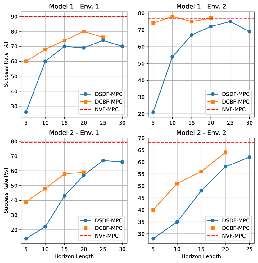
Figure 3: Results of the experiments with increased horizon lengths of the baselines.

Improved feasibility and performance: As noted in [26], including a constraint in the form Eq. 15 in an MPC can negatively impact feasibility depending on the parameter $\gamma$. Since the safety constraint in [26, Example A] is designed based on an SDF, it does not resemble the maximal safe set. In Fig. 4 we illustrate this by assuming the robot at state $x_{k}$ is moving toward $x_{goal}$ with an obstacle in between. We denote the forward reachable set at $k+1$ by $R_{k+1}$ (green region). Boundaries between estimated safe and unsafe regions at time step $k$ are denoted by $\partial S_{k}^{\gamma_{1}}$, $\partial S_{k}^{\gamma_{2}}$ and $\partial S_{k}^{\gamma_{3}}$ for ${\gamma_{1}<\gamma_{2}<\gamma_{3}}$, respectively. The optimizer needs to find $x_{k+1}$ from the intersection of the estimated safe region and $R_{k+1}$. For $\gamma_{3}$ the solution lies inside the BRT of the obstacle and will lead to a collision. For $\gamma_{1}$ the intersection is the empty set, rendering the problem infeasible. Only for $\gamma_{2}$ this approach provides a safe and feasible solution, but with suboptimal performance. On the other hand, the optimizer is able to find the near-optimal solution $x_{k+1}^{*}$ in our approach, which tends to have maximal progress and safety simultaneously.

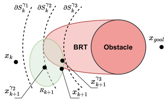
Figure 4: Illustration of improved feasibility and performance.

V-C Comparison with a Single-Network Architecture

In order to emphasize the benefits of a two-network model architecture, we compare our approach to the case when a single network is integrated as a constraint within an MPC planner approximating HJ value function based on local observations. As the baseline, we use the FC model proposed in [39]. The two approaches are compared for the 3-dimensional robot model (Model 2). In the case of a single-network architecture, the input is a vector consisting of costmap pixels and system states, while the output is the predicted HJ value function. The model is trained under the same settings as the hypernetwork in our approach. These experiments show significant advantages of our model architecture, both during training and deployment phase.

Computational efficiency: The primary advantage of our approach is emphasized during the deployment, i.e. when the model is integrated with the MPC planner and used for real-time trajectory optimization. As with our approach, the single-network model is integrated with the MPC planner using the CasADi framework. Based on the conducted experiments, we observe that the single-network architecture takes $\sim$10 s for trajectory optimization with a prediction horizon of 10 steps. In contrast, our NVF-MPC method takes $\sim$20 ms in the same case, which means that the computational efficiency is improved by three orders of magnitude.

Memory efficiency during the training phase: During the training process, we observe higher memory requirements for the single-network model compared to our approach. For the 3-dimensional dynamics, our model requires $\sim$1.68GB of memory for one forward and backward pass with a single training sample, while the single-network model requires $\sim$17.86GB of memory. This illustrates one order of magnitude improvement in terms of memory efficiency of the proposed architecture. This can be explained by the large number of state-space grid points propagated per every training sample. In our case the grid is propagated only through the main network, which is significantly less complex compared to the single-network model.

VI CONCLUSIONS

We presented a novel learning-based approach for approximating maximal safe sets in real time for local motion panning tasks. Our method uses a hypernetwork to parameterize a simple MLP model based on a binary costmap. The MLP model approximates the maximal safe set around the robot and it is used as a safety constraint for the MPC local planner. The model is trained based on the data generated offline via HJ reachability analysis. The results show the advantage of our approach in terms of increased success rate compared to the relevant baselines while still being real-time feasible. Also, the proposed model architecture greatly improves computational efficiency and requires less resources during training compared to the single-network architecture. In comparison with other methods for HJ value function estimation in unknown environments, our method can handle a high-dimensional environment representation.

The main theoretical limitation of our work is the lack of formal guarantees of safety, which is a common drawback of learning-based approaches [39]. At the same time, the technical challenge is the computational complexity of HJ reachability which scales exponentially with the model size. To improve scalability, one can use techniques such as state decomposition [52, 53] or neural solvers such as DeepReach [39] to directly support higher-dimensional systems. Therefore, providing formal analysis on safety and enhancing scalability remains the main direction for future work.

References

- [1] X. Zhang, A. Liniger, and F. Borrelli, “Optimization-Based Collision Avoidance,” Jun. 2018, arXiv:1711.03449 [cs, math]. [Online]. Available: http://arxiv.org/abs/1711.03449
- [2] T. Schoels, L. Palmieri, K. O. Arras, and M. Diehl, “An NMPC Approach using Convex Inner Approximations for Online Motion Planning with Guaranteed Collision Avoidance,” Feb. 2020, arXiv:1909.08267 [cs, eess, math]. [Online]. Available: http://arxiv.org/abs/1909.08267
- [3] C. Rosmann, F. Hoffmann, and T. Bertram, “Timed-Elastic-Bands for time-optimal point-to-point nonlinear model predictive control,” in 2015 European Control Conference (ECC). Linz, Austria: IEEE, Jul. 2015, pp. 3352–3357. [Online]. Available: http://ieeexplore.ieee.org/document/7331052/
- [4] G. Williams, P. Drews, B. Goldfain, J. M. Rehg, and E. A. Theodorou, “Aggressive driving with model predictive path integral control,” in 2016 IEEE International Conference on Robotics and Automation (ICRA). Stockholm: IEEE, May 2016, pp. 1433–1440. [Online]. Available: https://ieeexplore.ieee.org/document/7487277/
- [5] D. Fox, W. Burgard, and S. Thrun, “The dynamic window approach to collision avoidance,” IEEE Robotics & Automation Magazine, vol. 4, no. 1, pp. 23–33, Mar. 1997. [Online]. Available: http://ieeexplore.ieee.org/document/580977/
- [6] S. S. Samsani, H. Mutahira, and M. S. Muhammad, “Memory-based crowd-aware robot navigation using deep reinforcement learning,” Complex & Intelligent Systems, vol. 9, no. 2, pp. 2147–2158, Apr. 2023. [Online]. Available: https://doi.org/10.1007/s40747-022-00906-3
- [7] J. Tordesillas and J. P. How, “Deep-PANTHER: Learning-Based Perception-Aware Trajectory Planner in Dynamic Environments,” Feb. 2023, arXiv:2209.01268 [cs]. [Online]. Available: http://arxiv.org/abs/2209.01268
- [8] X. Xiao, T. Zhang, K. Choromanski, E. Lee, A. Francis, J. Varley, S. Tu, S. Singh, P. Xu, F. Xia, S. M. Persson, D. Kalashnikov, L. Takayama, R. Frostig, J. Tan, C. Parada, and V. Sindhwani, “Learning Model Predictive Controllers with Real-Time Attention for Real-World Navigation,” Sep. 2022, arXiv:2209.10780 [cs]. [Online]. Available: http://arxiv.org/abs/2209.10780
- [9] M.-K. Bouzidi, Y. Yao, D. Goehring, and J. Reichardt, “Learning-Aided Warmstart of Model Predictive Control in Uncertain Fast-Changing Traffic,” Oct. 2023, arXiv:2310.02918 [cs, eess]. [Online]. Available: http://arxiv.org/abs/2310.02918
- [10] K. P. Wabersich and M. N. Zeilinger, “A predictive safety filter for learning-based control of constrained nonlinear dynamical systems,” Automatica, vol. 129, p. 109597, Jul. 2021. [Online]. Available: https://www.sciencedirect.com/science/article/pii/S0005109821001175
- [11] K. P. Wabersich, A. J. Taylor, J. J. Choi, K. Sreenath, C. J. Tomlin, A. D. Ames, and M. N. Zeilinger, “Data-Driven Safety Filters: Hamilton-Jacobi Reachability, Control Barrier Functions, and Predictive Methods for Uncertain Systems,” IEEE Control Systems, vol. 43, no. 5, pp. 137–177, 2023. [Online]. Available: https://ieeexplore.ieee.org/document/10266799/
- [12] Y. Chen, A. Singletary, and A. D. Ames, “Guaranteed Obstacle Avoidance for Multi-Robot Operations With Limited Actuation: A Control Barrier Function Approach,” IEEE Control Systems Letters, vol. 5, no. 1, pp. 127–132, Jan. 2021. [Online]. Available: https://ieeexplore.ieee.org/document/9112342/
- [13] M. Zucker, J. Bagnell, C. Atkeson, and J. Kuffner, “An Optimization Approach to Rough Terrain Locomotion,” in IEEE International Conference on Robotics and Automation, May 2010, pp. 3589–3595.
- [14] M. N. Finean, W. Merkt, and I. Havoutis, “Predicted Composite Signed-Distance Fields for Real-Time Motion Planning in Dynamic Environments,” Mar. 2021, arXiv:2008.00969 [cs, eess]. [Online]. Available: http://arxiv.org/abs/2008.00969
- [15] M. Gaertner, M. Bjelonic, F. Farshidian, and M. Hutter, “Collision-Free MPC for Legged Robots in Static and Dynamic Scenes,” Mar. 2021, publication Title: arXiv e-prints ADS Bibcode: 2021arXiv210313987G. [Online]. Available: https://ui.adsabs.harvard.edu/abs/2021arXiv210313987G
- [16] H. Oleynikova, A. Millane, Z. Taylor, E. Galceran, J. Nieto, and R. Siegwart, “Signed Distance Fields: A Natural Representation for Both Mapping and Planning,” in RSS 2016 Workshop: Geometry and Beyond - Representations, Physics, and Scene Understanding for Robotics. ETH Zurich, 2016, p. 6 p.
- [17] H. Oleynikova, Z. Taylor, M. Fehr, J. Nieto, and R. Siegwart, “Voxblox: Incremental 3D Euclidean Signed Distance Fields for On-Board MAV Planning,” in 2017 IEEE/RSJ International Conference on Intelligent Robots and Systems (IROS), Sep. 2017, pp. 1366–1373, arXiv:1611.03631 [cs]. [Online]. Available: http://arxiv.org/abs/1611.03631
- [18] J. Ortiz, A. Clegg, J. Dong, E. Sucar, D. Novotny, M. Zollhoefer, and M. Mukadam, “iSDF: Real-Time Neural Signed Distance Fields for Robot Perception,” May 2022, arXiv:2204.02296 [cs]. [Online]. Available: http://arxiv.org/abs/2204.02296
- [19] V. Sitzmann, E. R. Chan, R. Tucker, N. Snavely, and G. Wetzstein, “MetaSDF: Meta-learning Signed Distance Functions,” Jun. 2020, arXiv:2006.09662 [cs]. [Online]. Available: http://arxiv.org/abs/2006.09662
- [20] D. Driess, J.-S. Ha, M. Toussaint, and R. Tedrake, “Learning Models as Functionals of Signed-Distance Fields for Manipulation Planning,” Oct. 2021, arXiv:2110.00792 [cs]. [Online]. Available: http://arxiv.org/abs/2110.00792
- [21] A. D. Ames, S. Coogan, M. Egerstedt, G. Notomista, K. Sreenath, and P. Tabuada, “Control Barrier Functions: Theory and Applications,” Mar. 2019, arXiv:1903.11199 [cs]. [Online]. Available: http://arxiv.org/abs/1903.11199
- [22] W. Xiao and C. Belta, “Control Barrier Functions for Systems with High Relative Degree,” Mar. 2019, arXiv:1903.04706 [cs]. [Online]. Available: http://arxiv.org/abs/1903.04706
- [23] P. Thontepu, B. G. Goswami, M. Tayal, N. Singh, S. P I, S. S. M. G, S. Sundaram, V. Katewa, and S. Kolathaya, “Control Barrier Functions in UGVs for Kinematic Obstacle Avoidance: A Collision Cone Approach,” Oct. 2023, arXiv:2209.11524 [cs, math]. [Online]. Available: http://arxiv.org/abs/2209.11524
- [24] J. Huang, Z. Liu, J. Zeng, X. Chi, and H. Su, “Obstacle Avoidance for Unicycle-Modelled Mobile Robots with Time-varying Control Barrier Functions,” Jul. 2023, arXiv:2307.08227 [cs]. [Online]. Available: http://arxiv.org/abs/2307.08227
- [25] H. Abdi, G. Raja, and R. Ghabcheloo, “Safe Control using Vision-based Control Barrier Function (V-CBF),” in 2023 IEEE International Conference on Robotics and Automation (ICRA). London, United Kingdom: IEEE, May 2023, pp. 782–788. [Online]. Available: https://ieeexplore.ieee.org/document/10160805/
- [26] J. Zeng, B. Zhang, and K. Sreenath, “Safety-Critical Model Predictive Control with Discrete-Time Control Barrier Function,” Mar. 2021, arXiv:2007.11718 [cs, eess]. [Online]. Available: http://arxiv.org/abs/2007.11718
- [27] N. N. Minh, S. McIlvanna, Y. Sun, Y. Jin, and M. Van, “Safety-critical model predictive control with control barrier function for dynamic obstacle avoidance,” Nov. 2022, arXiv:2211.11348 [cs, eess]. [Online]. Available: http://arxiv.org/abs/2211.11348
- [28] Z. Jian, Z. Yan, X. Lei, Z. Lu, B. Lan, X. Wang, and B. Liang, “Dynamic Control Barrier Function-based Model Predictive Control to Safety-Critical Obstacle-Avoidance of Mobile Robot,” Sep. 2022, arXiv:2209.08539 [cs]. [Online]. Available: http://arxiv.org/abs/2209.08539
- [29] Z. Zhang, Q. Zhao, and K. Sun, “A Learning-Based Method for Computing Control Barrier Functions of Nonlinear Systems With Control Constraints,” IEEE Robotics and Automation Letters, vol. 8, no. 7, pp. 4259–4266, Jul. 2023. [Online]. Available: https://ieeexplore.ieee.org/document/10141659/
- [30] S. Liu, C. Liu, and J. Dolan, “Safe Control Under Input Limits with Neural Control Barrier Functions,” Nov. 2022, arXiv:2211.11056 [cs, eess]. [Online]. Available: http://arxiv.org/abs/2211.11056
- [31] O. So, Z. Serlin, M. Mann, J. Gonzales, K. Rutledge, N. Roy, and C. Fan, “How to Train Your Neural Control Barrier Function: Learning Safety Filters for Complex Input-Constrained Systems,” Dec. 2023, arXiv:2310.15478 [cs, math]. [Online]. Available: http://arxiv.org/abs/2310.15478
- [32] J. Lee, J. Kim, and A. D. Ames, “A Data-driven Method for Safety-critical Control: Designing Control Barrier Functions from State Constraints,” Dec. 2023, arXiv:2312.07786 [cs] version: 1. [Online]. Available: http://arxiv.org/abs/2312.07786
- [33] M. Srinivasan, A. Dabholkar, S. Coogan, and P. Vela, “Synthesis of Control Barrier Functions Using a Supervised Machine Learning Approach,” Mar. 2020, arXiv:2003.04950 [cs, eess]. [Online]. Available: http://arxiv.org/abs/2003.04950
- [34] K. Long, C. Qian, J. Cortés, and N. Atanasov, “Learning Barrier Functions with Memory for Robust Safe Navigation,” Feb. 2021, arXiv:2011.01899 [cs]. [Online]. Available: http://arxiv.org/abs/2011.01899
- [35] C. Li, Z. Zhang, A. Nesrin, Q. Liu, F. Liu, and M. Buss, “Instantaneous Local Control Barrier Function: An Online Learning Approach for Collision Avoidance,” Jan. 2022, arXiv:2106.05341 [cs, eess]. [Online]. Available: http://arxiv.org/abs/2106.05341
- [36] Z. Li, “Comparison between safety methods control barrier function vs. reachability analysis,” Jun. 2021, arXiv:2106.13176 [cs, eess]. [Online]. Available: http://arxiv.org/abs/2106.13176
- [37] S. Bansal, M. Chen, S. Herbert, and C. J. Tomlin, “Hamilton-Jacobi Reachability: A Brief Overview and Recent Advances,” Sep. 2017, arXiv:1709.07523 [cs, math]. [Online]. Available: http://arxiv.org/abs/1709.07523
- [38] R. E. Allen, A. A. Clark, J. A. Starek, and M. Pavone, “A machine learning approach for real-time reachability analysis,” in 2014 IEEE/RSJ International Conference on Intelligent Robots and Systems. Chicago, IL, USA: IEEE, Sep. 2014, pp. 2202–2208. [Online]. Available: http://ieeexplore.ieee.org/document/6942859/
- [39] S. Bansal and C. Tomlin, “DeepReach: A Deep Learning Approach to High-Dimensional Reachability,” Nov. 2020, arXiv:2011.02082 [cs, eess]. [Online]. Available: http://arxiv.org/abs/2011.02082
- [40] J. Borquez, K. Nakamura, and S. Bansal, “Parameter-Conditioned Reachable Sets for Updating Safety Assurances Online,” in 2023 IEEE International Conference on Robotics and Automation (ICRA), May 2023, pp. 10 553–10 559, arXiv:2209.14976 [cs, eess]. [Online]. Available: http://arxiv.org/abs/2209.14976
- [41] H. J. Jeong, Z. Gong, S. Bansal, and S. Herbert, “Parameterized Fast and Safe Tracking (FaSTrack) using Deepreach,” Apr. 2024, arXiv:2404.07431 [cs, eess]. [Online]. Available: http://arxiv.org/abs/2404.07431
- [42] K. Nakamura and S. Bansal, “Online Update of Safety Assurances Using Confidence-Based Predictions,” Jun. 2023, arXiv:2210.01199 [cs]. [Online]. Available: http://arxiv.org/abs/2210.01199
- [43] A. Bajcsy, S. Bansal, E. Bronstein, V. Tolani, and C. J. Tomlin, “An Efficient Reachability-Based Framework for Provably Safe Autonomous Navigation in Unknown Environments,” May 2019, arXiv:1905.00532 [cs]. [Online]. Available: http://arxiv.org/abs/1905.00532
- [44] G. Chou, N. Ozay, and D. Berenson, “Uncertainty-Aware Constraint Learning for Adaptive Safe Motion Planning from Demonstrations,” Nov. 2020, arXiv:2011.04141 [cs, eess]. [Online]. Available: http://arxiv.org/abs/2011.04141
- [45] C. Richter, W. Vega-Brown, and N. Roy, “Bayesian Learning for Safe High-Speed Navigation in Unknown Environments,” in Robotics Research, A. Bicchi and W. Burgard, Eds. Cham: Springer International Publishing, 2018, vol. 3, pp. 325–341.
- [46] E. N. Barron, “Differential games with maximum cost,” Nonlinear Analysis: Theory, Methods & Applications, vol. 14, no. 11, pp. 971–989, Jun. 1990. [Online]. Available: https://www.sciencedirect.com/science/article/pii/0362546X9090113U
- [47] J. F. Fisac, M. Chen, C. J. Tomlin, and S. S. Sastry, “Reach-Avoid Problems with Time-Varying Dynamics, Targets and Constraints,” Oct. 2014, arXiv:1410.6445 [math]. [Online]. Available: http://arxiv.org/abs/1410.6445
- [48] D. Ha, A. Dai, and Q. V. Le, “HyperNetworks,” Dec. 2016, arXiv:1609.09106 [cs]. [Online]. Available: http://arxiv.org/abs/1609.09106
- [49] V. K. Chauhan, J. Zhou, P. Lu, S. Molaei, and D. A. Clifton, “A Brief Review of Hypernetworks in Deep Learning,” Aug. 2023, arXiv:2306.06955 [cs]. [Online]. Available: http://arxiv.org/abs/2306.06955
- [50] T. Galanti and L. Wolf, “On the Modularity of Hypernetworks,” in Advances in Neural Information Processing Systems, vol. 33. Curran Associates, Inc., 2020, pp. 10 409–10 419.
- [51] J. A. E. Andersson, J. Gillis, G. Horn, J. B. Rawlings, and M. Diehl, “CasADi: a software framework for nonlinear optimization and optimal control,” Mathematical Programming Computation, vol. 11, no. 1, pp. 1–36, Mar. 2019. [Online]. Available: http://link.springer.com/10.1007/s12532-018-0139-4
- [52] M. Chen, S. Herbert, and C. J. Tomlin, “Exact and Efficient Hamilton-Jacobi-based Guaranteed Safety Analysis via System Decomposition,” Sep. 2016, arXiv:1609.05248 [math]. [Online]. Available: http://arxiv.org/abs/1609.05248
- [53] S. Herbert, J. J. Choi, S. Sanjeev, M. Gibson, K. Sreenath, and C. J. Tomlin, “Scalable Learning of Safety Guarantees for Autonomous Systems using Hamilton-Jacobi Reachability,” Apr. 2021, arXiv:2101.05916 [cs, eess]. [Online]. Available: http://arxiv.org/abs/2101.05916