Experimental demonstration of the Bell-type inequalities for four qubit Dicke state using IBM Quantum Processing Unit

Abstract

Violation of the Bell-type inequalities is very necessary to confirm the existence of the nonlocality in the nonclassical (entangled) states. We have designed a customized operator which is made of the sum of the identity and Pauli matrices ($I$, $\sigma_{x}$, $\sigma_{y}$, and $\sigma_{z}$). We theoretically evaluate the Bell-type violation for the two-qubit Bell state and a four-qubit Dicke state, which gives the Bell-CHSH parameter values $2\sqrt{2}$ and $3.05$, respectively for our customized operator. For experimental implementation, IBM’s 127-qubitQuantum Processing Units (QPU) were utilized, where we have applied our customized operator to evaluate Bell-type inequalities for two-qubit Bell state ($|\Phi^{+}\rangle$) and four-qubit Dicke state ($|D^{(2)}_{4}\rangle$). We observed, for the two-qubit Bell state, the experimental Bell violation was $2.7507\pm 0.0197$. For Dicke state, we found the violation be to $2.1239\pm 0.0457$ and $2.2175\pm 0.0352$ respectively for two distinct methods of state preparation. All our results show clear violation of the local realism; however, we find that the experimental violation of the Bell state ($2.75$) is close to the theoretical ($2.82$) results due to lower circuit depth in state-preparation as well as fewer measurements, while the Dicke state shows greater errors ($2.12$ and $2.21$ vs. $3.05$) from higher depth and more measurements.

Keywords-Bell states, Dicke State, IBM quantum computer, Customized Operator, Bell-type inequality, etc.

I Introduction

Quantum entanglement is an essential phenomenon in quantum information because of its correlation between two (or many) particles [1]. Quantum entanglement is a key component in many quantum information processing techniques such as quantum teleportation [2, 3], quantum dense coding [4, 5], quantum cryptography [6, 7]. Regarding quantum entanglement, the two-qubit (two-partite) Bell state has received much attention, but the multipartite entangled state and its applications are also gaining investigators’ attention. High-quality multipartite entangled states, such as Greenberger-Horne-Zeilinger (GHZ) states [7], W states, Cluster states, and Dicke states, are very important because they play a vital role in quantum information theory and its applications. Therefore, the efficient way of experimental generation of these states is very challenging and violations of local hidden variable theory for multipartite entangled states are also critical for certain device-independent (DI) quantum information processing tasks, including ensuring the security of quantum key distribution (QKD) [8, 9], reducing computational complexity [10, 11], and validating random number generation [12]. Detecting violations of local realism in multipartite correlations presents significant challenges, primarily due to the absence of straightforward Bell inequalities for multipartite systems. In the case of two-qubit systems, the Clauser-Horne-Shimony-Holt (CHSH) inequality [13] is relatively simple in form, which facilitates the experimental observation of violations of local hidden variable theories. For systems involving any number of observers, a selection between two local dichotomic observables is chosen for which researchers have developed a comprehensive set of CHSH Bell type of inequalities [14, 15, 16]. These inequalities exhibit a unified structure [17]. Despite this, the explicit forms of Bell inequalities are frequently too intricate to effectively confirm violations of local realism. A multipartite Mermin-Ardehali-Belinskii-Klyshko (MABK) inequalities do provide explicit expressions; however, for an $N$-partite system, these inequalities require consideration of $2N$ terms [18, 19, 20]. The complexity of MABK inequalities makes them less practical for testing the nonlocality of multipartite entangled states, particularly as the number of particles increases. However, multipartite Bell inequalities that focus solely on two-body correlations can still detect Bell nonlocality in many-body systems. This approach provides a viable pathway for experimentally verifying multipartite Bell nonlocality [21, 22].

Reducing the number of terms in a Bell inequality simplifies the demonstration of nonlocality for multipartite entangled states. Through an analysis of the geometrical properties of correlation polytopes, researchers have uncovered structural characteristics of CHSH-type Bell inequalities [23]. Additionally, multipartite CHSH-type Bell inequalities with few terms have been proposed, facilitating the experimental approaches to detect violations of local realism in multipartite entangled states. Dicke states, which naturally occur in symmetric systems [24], exhibit strong resilience against photon loss and projective measurements [25] and have a high degree of multipartite entanglement. Researchers have observed that Dicke states are ideal for quantum metrology [26, 27] and are useful for quantifying the entanglement depth in many-body systems [28]. These favorable properties have spurred considerable efforts to produce high-quality Dicke states. For instance, in optical systems, a four-photon symmetric Dicke state with a fidelity of $0.844\pm 0.008$ was experimentally realized by N. Kiesel et al. in 2007 [25], and $0.904\pm 0.004$ by Yuan Yuan Zhao et al. in 2015 [29] while the six-photon version was concurrently achieved by W. Wieczorek et al. [30] and R. Prevedel et al. [31]. However, conventional methods for detecting the entanglement of Dicke states do not always indicate violations of local realism [25, 26, 30, 31, 32].

In this work, we discuss the generation of the four-qubit Dicke state and the violation of the Bell-type inequality [33] using our custom operators [34]. To violate the Bell-type inequality for bipartite and multipartite entangled states, a specific basis for the corresponding state and inequality is required. Our customized operator is basis-independent and can be directly employed to determine the violation of the Bell inequality for both two-qubit and multi-qubit systems.

In order to implement the custom operators on IBM QPU, we decompose them in terms of identity and Pauli matrices ($I$, $\sigma_{x}$, $\sigma_{y}$, and $\sigma_{z}$) with appropriate coefficients. This decomposed representation can then be implemented directly on the IBM Quantum Processing Units (QPUs). To test and simulate quantum algorithms, IBM Quantum has made its QPUs available to the public since 2016. IBM Quantum provides a cloud-based access to QPUs that enables users to design and test quantum circuits on both simulators and real QPUs. IBM’s Composer is a cloud-based platform for quantum computing, accessible through their website. It allows users to build quantum circuits which then can be executed either on a simulator or a quantum processing unit (QPU) via a cloud interface:( https://quantum.ibm.com/). Numerous quantum chip experiments have now been conducted using IBM QPUs. Quantum simulation [35, 36], the creation of quantum algorithms [37], the testing of theoretical problems involving quantum information [38], quantum cryptography [39], quantum error correction [40], and quantum applications [41] are just a few examples of actual experiments. Initially, we evaluated the Bell-violation for the two-qubit Bell state using our customized operator on IBM’s QPU, as well as on the fake-backend (noisy simulator) which replicates the features and noise characteristics of the actual IBM quantum devices[42] to complement the real hardware runs we executed. Subsequently, a four-qubit Dicke state was prepared and its local realism was investigated by incorporating the aforementioned methodology.

The remainder of this article is organized as follows: in Sec. II, we describe the two distinct methods for generating the Dicke state. The development of our customized operator is outlined in Sec. III. Experimental implementation is discussed in Sec. IV. Our findings are presented in Sec. V, and we conclude the article in Sec. VI.

II Generation of four qubit Dicke state

A four-qubit Dicke state is a specific type of quantum state involving four qubits that exhibit a particular entanglement pattern. Four qubit Dicke state was introduced in the context of studying superradiance. Mathematically, the four-qubit Dicke state is written in the following form

$$|D^{(2)}_{4}\rangle=\frac{1}{\sqrt{6}}\left(|0011\rangle+|0101\rangle+|1001\rangle\right.\\ \left.+|0110\rangle+|1010\rangle+|1100\rangle\right)$$ (1)

Here, $|0\rangle$ and $|1\rangle$ represent the computational basis. The Dicke state is a widely used type of multi-partite entangled state in quantum information. However, very few works have been done on there nonlocality test. The test of nonlocality was carried out by generating the Dicke state by two distinct methods on IBM QPU.

II.1 Unitary Gate Based Initialization

We generated the Bell state ($|\Phi^{+}$) by utilizing the Hadamard and CNOT gate. The same gate-based approach can be extended for the Dicke state as reported in [43]. In this method, the construction of the Dicke state was implemented by a precise sequence of quantum gates, mainly via a combination of single-qubit rotations and controlled-NOT (CNOT) as shown in Fig. 1. However, we made slight modifications to the rotation angles of the $"Ry"$ gates as compared to the state generation as discussed in [43]. These modifications were necessary to generate the precise Dicke state as described in Eq. (1)., which closely resembles the theoretical Dicke state with minimal deviation.

II.2 State vector Based Initialization

The generation of the Dicke state utilizes the framework established in [44]. This method directly generates a circuit that prepares the specified Dicke state by constructing a state vector and deriving the associated quantum circuit that fulfills the generation of this vector. This technique considers the Dicke state as an isometry from a lower-dimensional Hilbert space, which may be effectively decomposed into a series of single-qubit and CNOT gates Fig. 3. This method provides a more direct approach to achieving the desired state, without the necessity of fine-tuning gate parameters as necessary in gate-based method, and guarantees that the created quantum state is more precise.

Fig. 2. illustrates the procedure for measuring the $XXYZ$ measurement configuration in the Dicke state ($|D^{(2)}_{4}\rangle$) using the configured quantum circuit. Likewise, we have conducted the necessary measurements in order to violate the Bell inequality by altering the corresponding gates. The identical methodology is employed for circuits constructed via state-vector based method.

The method in [23] devised the Bell inequality we construct. The inequality is given by

$$|\hat{A}\hat{B}\hat{C}\hat{D}+\hat{A}\hat{B}^{\prime}\hat{C}^{\prime}\hat{D}^{\prime}\\ +\hat{A}^{\prime}\hat{B}\hat{C}^{\prime}\hat{D}-\hat{A}^{\prime}\hat{B}^{\prime}\hat{C}\hat{D}^{\prime}|\leq 2.$$ (2)

Where, The local observables $\hat{A}_{i}$, $\hat{B}_{i}$, $\hat{C}_{i}$, and $\hat{D}_{i}$ have the form: $\hat{X}_{i}=\mathbf{x}_{i}\cdot\bm{\sigma}$, where $\mathbf{x}_{i}=(x_{i1},x_{i2},x_{i3})\in\mathbb{R}^{3}$ with $|\mathbf{x}_{i}|=1$ (for $i=0,1$), and the Pauli operator is given by $\bm{\sigma}=(I,\sigma_{x},\sigma_{y},\sigma_{z})$.

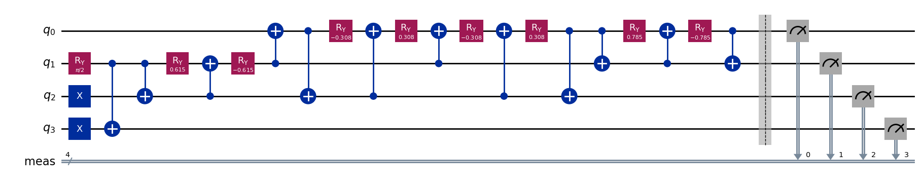
Figure 1: Illustration of a 4-qubit Dicke State ($|D^{(2)}_{4}\rangle$) state construction using gate based method.

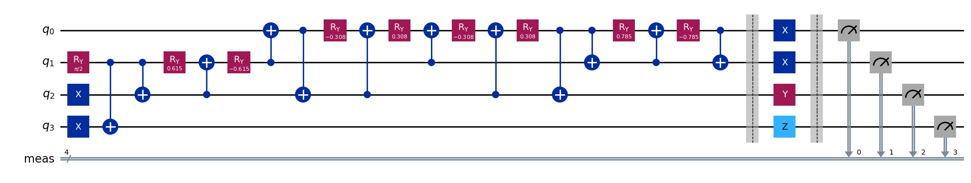
Figure 2: Illustration of circuit to find Expectation value of operator XXYZ over 4 qubit Dicke state ($|D^{(2)}_{4}\rangle$).

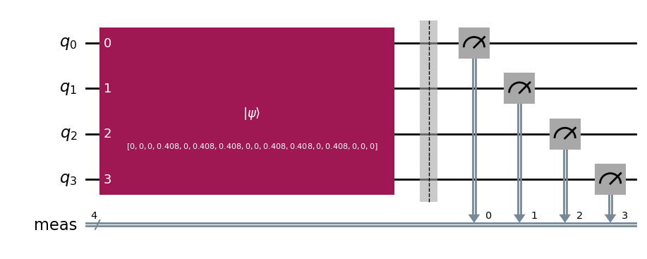
Figure 3: Illustration of a 4-qubit Dicke State ($|D^{(2)}_{4}\rangle$) state construction using state-vector based method.

III Development of Customized Operator

To get the maximal violation of any Bell-type inequalities, we are assigning a local arbitrary observable in the form of a general operator $\bm{\hat{X}_{\hat{n}}}=x_{i}.\bm{\hat{\sigma}}$ where $x_{i}=(x_{0},x_{1},x_{2},x_{3})\in\mathbb{R}^{4}$ with $\sum_{i=0}^{3}x_{i}^{2}=1$ and Pauli operator $\bm{\hat{\sigma}}=(\hat{\mathbf{I}},\hat{\bm{\sigma}_{x}},\hat{\bm{\sigma}_{y}},\hat{\bm{\sigma}_{z}})$. In a four-dimensional spherical space $\bm{\hat{X}_{\hat{n}}}$ can be represented as,

$$\bm{\hat{X}_{\hat{n}}}=\cos(\gamma)\hat{\mathbf{I}}-\sin(\gamma)\Big{[}\sin(\theta)\cos(\phi)\hat{\bm{\sigma}}_{x}\\ +\sin(\theta)\sin(\phi)\hat{\bm{\sigma}}_{y}+\cos(\theta)\hat{\bm{\sigma}}_{z}\Big{]}$$ (3)

where $\phi\in(0,2\pi),\theta\in(0,\pi),\gamma\in(0,\pi)$ are arbitrary angle spanning the four dimensional space. Using the above operator, we will show that for the two-qubit Bell state and four-qubit Dicke state violate the Bell-type inequality both theoretically and experimentally on an IBM QPU.

III.1 Maximum violation bound for two-qubit $|\Phi^{+}\rangle$ Bell state

Here, we have derived the maximal violation condition for the maximally entangled two-qubit $|\Phi^{+}\rangle$ Bell state, which is written as,

$$|\Phi^{+}\rangle=\frac{1}{\sqrt{2}}|00\rangle+|11\rangle,$$ (4)

where $|0\rangle$ and $|1\rangle$ represent the computational basis. The CHSH Bell inequality [45] for two-particle has the following form,

$$|S_{|\Phi^{+}\rangle}|=|\langle\hat{A}\hat{B}\rangle+\langle\hat{A}\hat{B^{\prime}}\rangle-\langle\hat{A^{\prime}}\hat{B}\rangle+\langle\hat{A^{\prime}}\hat{B^{\prime}}\rangle|\leq 2,$$ (5)

where $\hat{A}(\hat{A^{\prime}})$ and $\hat{B}(\hat{B^{\prime}})$ are the arbitrary possible choices of measurements on particles 1 and 2, respectively. The verification procedure relies on computing all correlation functions, e.g.$\langle\hat{A}\hat{B}\rangle$. The observable $\langle\hat{A}\hat{B}\rangle$ represents the expectation value of the joint probability of outcomes of measurements $\hat{A}$ and $\hat{B}$ on particle 1 and 2, respectively. Calculating all such terms appearing in Eq.(5) leads to the algebraic expression of the Bell polynomial. The value is then compared to the predicted value using local realism. In the domain of quantum mechanics, the measurements specified in Eq.(5) can be regarded as polarization measurements and are specified by the linear combination of Pauli operators in Eq.(3). The quantum mechanical expectation value specified in $1^{st}$ term of Eq.(5) can be calculated for $|\Phi^{+}\rangle$ Bell state as,

$$\langle\hat{A}\hat{B}\rangle =\langle\Phi^{+}|\bm{\hat{X}_{\hat{n}_{A}}}\otimes\bm{\hat{X}_{\hat{n}_{B}}}|\Phi^{+}\rangle$$

$$=\cos(\gamma_{A})\cos(\gamma_{B})+\sin(\gamma_{A})\sin(\gamma_{B})[\cos(\theta_{A})$$

$$\cos(\theta_{B})+\cos(\phi_{A}+\phi_{B})\sin(\theta_{A})\sin(\theta_{B})],$$ (6)

where $\phi_{i}(\phi_{i}^{\prime})$, $\theta_{i}(\theta_{i}^{\prime})$, $\gamma_{i}(\gamma_{i}^{\prime})$ $\forall i\in(A,B)$ are polar angles specifying the measurement direction $\hat{n}_{i},(\hat{n}_{i}^{\prime})$. Similarly, after calculating other terms in Eq.(5), we derived the Bell polynomial as shown in Eq.(A).

To get the values of polar angles corresponding to the maximal violation, we are required to maximize the Bell polynomial calculated in Eq.(A) using Mathematica^®. There is more than one optimum condition, out of which one condition is shown in Table (1). By substituting the values of polar angles shown in Table (1) in Eq.(A), we got the Bell value $|S_{|\Phi^{+}\rangle}|=2\sqrt{2}$.

$\theta_{A}=116.40^{\circ}$	$\theta_{A}^{\prime}=20.51^{\circ}$	$\theta_{B}=17.16^{\circ}$	$\theta_{B}^{\prime}=127.08^{\circ}$
$\phi_{A}=91.55^{\circ}$	$\phi_{A}^{\prime}=51.33^{\circ}$	$\phi_{B}=51.57^{\circ}$	$\phi_{B}^{\prime}=103.60^{\circ}$
$\gamma_{A}=38.92^{\circ}$	$\gamma_{A}^{\prime}=81.88^{\circ}$	$\gamma_{B}=63.24^{\circ}$	$\gamma_{B}^{\prime}=49.45^{\circ}$

Table 1: Value of optimum angles to get maximal violation for the two-qubit Bell state $|\Phi^{+}\rangle$.

Using the given angle in Table 1, we calculated our customized operator in the form of Eq. 3 and given below

$$\bm{\hat{A}} =0.778067\hat{\mathbf{I}}+0.0151954i\hat{\bm{\sigma}}_{x}$$ (7)

$$\quad-0.562482i\hat{\bm{\sigma}}_{y}+0.279275i\hat{\bm{\sigma}}_{z},$$

$$\bm{\hat{B}}=0.450299\hat{\mathbf{I}}-0.164004i\hat{\bm{\sigma}}_{x}$$ (8)

$$-0.206226i\hat{\bm{\sigma}}_{y}-0.853114i\hat{\bm{\sigma}}_{z},$$

$$\bm{\hat{A^{\prime}}}=0.141248\hat{\mathbf{I}}-0.216741i\hat{\bm{\sigma}}_{x}$$ (9)

$$-0.270836i\hat{\bm{\sigma}}_{y}-0.927211i\hat{\bm{\sigma}}_{z},$$

$$\bm{\hat{B^{\prime}}}=0.650054\hat{\mathbf{I}}+0.142515i\hat{\bm{\sigma}}_{x}$$ (10)

$$-0.589245i\hat{\bm{\sigma}}_{y}+0.45816i\hat{\bm{\sigma}}_{z}.$$

We implemented these above operators on two qubit Bell state and executed on IBM QPU and shown bell violation.

III.2 Maximum violation bound for Four-qubit Dicke state

By extending our approach to higher qubits, we took four qubit Dicke state ($|D^{(2)}_{4}\rangle$) in this section to get the violation of four qubits Bell inequality. The four qubit Dicke state ($|D^{(2)}_{4}\rangle$) is defined in Eq. 1. The Bell-type inequality for the $|D^{(2)}_{4}\rangle$ state is defined in Eq.2, where $A(A^{\prime})$,$B(B^{\prime})$,$C(C^{\prime})$ and $D(D^{\prime})$ are the arbitrary possible choice of measurements on particle 1, 2, 3, and 4 respectively. Similarly, we calculated quantum mechanical expectation values of all terms given in Eq.(2) to find the value of Bell-Polynomial for $|D^{(2)}_{4}\rangle$ state. We calculated the quantum mechanical expectation value of the $1^{st}$ term of Eq.(2), and same is given in the Eq. (21).

Similarly, we calculated all four terms present in Eq.(2). After the simplification, by employing Mathematica^®for finding the polar angles corresponding to the maximum violation of the four qubit Dicke state. Similarly, we calculated the polar angles in which maximum violation for the qubits Dicke state occurred as we did for the two-qubit state. Theoretically, the maximum violation for Dicke state is 3.05. From the Polar angles calculated from the above equation, we construct the eight customized operators for violating Bell inequality in IBM qiskit. These eight operators are given below,

$$\bm{\hat{A}} =0.870984\hat{\mathbf{I}}+0.166552i\hat{\bm{\sigma}}_{x}$$ (11)

$$\quad+0.255672i\hat{\bm{\sigma}}_{y}-0.38507i\hat{\bm{\sigma}}_{z},$$

$$\bm{\hat{B}} =0.870852\hat{\mathbf{I}}+0.166799i\hat{\bm{\sigma}}_{x}$$ (12)

$$\quad+0.256052i\hat{\bm{\sigma}}_{y}-0.385009i\hat{\bm{\sigma}}_{z},$$

$$\bm{\hat{C}} =0.463311\hat{\mathbf{I}}-0.470613i\hat{\bm{\sigma}}_{x}$$ (13)

$$\quad-0.722433i\hat{\bm{\sigma}}_{y}-0.204833i\hat{\bm{\sigma}}_{z},$$

$$\bm{\hat{D}} =0.870852\hat{\mathbf{I}}+0.166799i\hat{\bm{\sigma}}_{x}$$ (14)

$$\quad+0.256052i\hat{\bm{\sigma}}_{y}-0.385009i\hat{\bm{\sigma}}_{z},$$

$$\bm{\hat{A^{\prime}}} =0.46222\hat{\mathbf{I}}-0.470995i\hat{\bm{\sigma}}_{x}$$ (15)

$$\quad-0.72302i\hat{\bm{\sigma}}_{y}-0.204351i\hat{\bm{\sigma}}_{z},$$

$$\bm{\hat{B^{\prime}}} =0.854403\hat{\mathbf{I}}-0.194754i\hat{\bm{\sigma}}_{x}$$ (16)

$$\quad-0.298964i\hat{\bm{\sigma}}_{y}-0.377739i\hat{\bm{\sigma}}_{z},$$

$$\bm{\hat{C^{\prime}}} =0.870736\hat{\mathbf{I}}+0.167013i\hat{\bm{\sigma}}_{x}$$ (17)

$$\quad+0.25638i\hat{\bm{\sigma}}_{y}-0.38496i\hat{\bm{\sigma}}_{z},$$

$$\bm{\hat{D^{\prime}}} =0.854403\hat{\mathbf{I}}-0.194754i\hat{\bm{\sigma}}_{x}$$ (18)

$$\quad-0.298964i\hat{\bm{\sigma}}_{y}-0.377739i\hat{\bm{\sigma}}_{z}.$$

IV Experimental Implementation

In this section, we discuss the implementation of our customized operator for violation of the Bell-type inequalities for the two-qubit Bell state and as well as four qubits Dicke state. Firstly, we discuss the two qubits, and then we extend our approach to the four qubits state.

IV.1 Two qubit Bell state implementation

Two-qubit Bell inequality experiment can be performed using different measurement setting. These measurement settings are typically represented by the operators $A$, $B$, $A^{\prime}$, and $B^{\prime}$ acting on the first and second qubits, respectively. To evaluate quantum inequalities such as those tested in this experiment, we decompose the operators $A$, $B$, $A^{\prime}$, and $B^{\prime}$ in terms of the identity matrix and the Pauli operators. Each operator is expressed as given in the Eq. (3). Where, $I$ represents the $2\times 2$ identity matrix, and $\sigma_{x}$, $\sigma_{y}$, and $\sigma_{z}$ are the Pauli matrices. This decomposition allows us to express each operator as a linear combination of fundamental quantum operations, enabling a more systematic way to compute expectation values and test for inequality violations. The expression of these operators is given in Eq. (7-10).

Since each operator is decomposed in terms of four matrices (the identity and the three Pauli matrices), the tensor product of two operators (e.g., $A\otimes B$) results in a total of 16 unique operators.

$$k_{i}k_{j}=k_{i}\otimes k_{j},\quad\text{where }k_{i},k_{j}\in\{I,\sigma_{x},\sigma_{y},\sigma_{z}\}$$

Such as $I\otimes I$, $I\otimes\sigma_{x}$, $I\otimes\sigma_{y}$, … , $\sigma_{z}\otimes\sigma_{z}$. Each operator corresponds to a distinct combination of measurements on the two qubits, enabling the calculation of expectation values for every pair of measurement configurations. However, not all these operators contribute equally to the quantum state under study, so we need to identify those that yield non-zero expectation values. To make this process more efficient, we compute the expectation value of each operator when acting on the two-qubit Bell state $|\Phi^{+}\rangle$. Through this analysis, we find that only four operators $II,XX,YY,ZZ$ have non-zero expectation values. These operators are, therefore, sufficient for our analysis and significantly reduce the computational overhead.

IV.1.1 Qiskit Implementation

After identifying the relevant operators, the implementation of the inequality violation test was carried out using Qiskit, which is a comprehensive open-source quantum computing framework[46]. We implemented the experiment using the Sampler primitive in Qiskit’s IBM Quantum runtime. The quantum circuit is constructed to prepare the desired entangled Bell state, followed by the application of the decomposed operators. We use Qiskit’s transpiler to optimize the circuit with optimization level 3, minimizing the circuit depth and reducing the number of two-qubit gates. This transpilation step is crucial in mitigating noise and improving the fidelity of the results, especially when running the circuit on real quantum hardware.

The optimized circuits are then executed on the IBM QPU, with each circuit being sampled 10,000 times to gather sufficient statistics for the calculation of expectation values. This high shot count ensures that the computed expectation values are robust against statistical fluctuations, allowing for more accurate testing of the quantum inequality. To complement the real hardware runs the experiments were also simulated on noisy simulators, which replicates the features and noise characteristics of the actual IBM QPU [42]. Usage of the noisy simulator enabled multiple runs without limitations on hardware access.

IV.1.2 Expectation Value Calculation from Measurement Counts

The expectation value of an operator is crucial for evaluating the inequality in question, as it directly reflects how the quantum state responds to different measurement settings.

After executing the quantum circuits on the real IBM QPU, the results are returned as a set of measurement counts. These counts represent how many times each possible outcome (bitstring) is measured in the given number of shots (repetitions of the circuit). For a two-qubit system, the possible outcomes are the bitstrings ‘00‘, ‘01‘, ‘10‘, and ‘11‘, corresponding to the measurement of the computational basis states $|00\rangle$, $|01\rangle$, $|10\rangle$, and $|11\rangle$, respectively.

IV.1.3 Mapping Counts to Expectation Values

To calculate the expectation value of an operator $X$, we use the measured counts to compute the probability of each outcome. The expectation value is then given by:

$$\langle X\rangle=\sum_{\text{outcomes}}P(\text{outcome})\cdot\text{eigenvalue(outcome)}$$

where $P(\text{outcome})$ is the probability of measuring a specific bitstring, and the corresponding eigenvalue depends on the operator and the outcome. For Pauli operators, the eigenvalues are $\pm 1$, as each Pauli matrix has eigenvalues in this range when measured in its eigenbasis.

For example, when measuring the Pauli-$Z$ operator on a qubit, the outcomes ‘0‘ and ‘1‘ correspond to eigenvalues $+1$ and $-1$, respectively. Thus, the expectation value of $Z$ is calculated as:

$$\langle Z\rangle=P(0)\cdot(+1)+P(1)\cdot(-1)=P(0)-P(1)$$

where $P(0)$ and $P(1)$ are the probabilities of measuring ‘0’ and ‘1’, respectively.

In the case of two-qubit operators like $\sigma_{x}\otimes\sigma_{x}$, the outcomes correspond to eigenvalues derived from the product of the eigenvalues of the individual Pauli operators acting on each qubit. For instance, the outcome ‘00’ would correspond to eigenvalue $+1\cdot+1=+1$, while the outcome ‘11’ would correspond to $-1\cdot-1=+1$. For each operator, we map each possible bitstring to its corresponding eigenvalue, then compute the expectation value as a weighted sum over the measurement probabilities.

IV.1.4 Correcting for Noise and Mitigating Errors

We have investigated the effect due to the various noise sources, such as gate errors, measurement errors, and decoherence in the raw counts obtained from the quantum circuit on the quantum backend. To account for this, we apply error mitigation techniques such as matrix-free measurement mitigation (MThree) to improve the accuracy of the expectation values [47]. This involves calibrating the backend to estimate and correct for measurement errors. Once these corrections are applied, the resulting quasi-probabilities are used to recalculate the counts, providing a more reliable estimate of the true measurement probabilities.

The corrected expectation value for each operator is then calculated as described above, using the mitigated counts to compute the probabilities of each outcome. For example, if we measure the operator $\sigma_{x}\otimes\sigma_{x}$ and obtain corrected counts {‘00’: 5000, ‘01’: 0, ‘10’: 0, ‘11’: 5000} out of 10,000 shots, the expectation value is:

$$\langle XX\rangle=\frac{5000}{10000}\cdot(+1)+\frac{5000}{10000}\cdot(+1)=1$$

This process is repeated for all operators of interest, such as $\sigma_{y}\otimes\sigma_{y}$ and $\sigma_{z}\otimes\sigma_{z}$, allowing us to compute their respective expectation values.

IV.1.5 Summing Contributions from Decomposed Operators

As we have decomposed the operators $A$, $B$, $A^{\prime}$, and $B^{\prime}$ into linear combinations of Pauli operators, the overall expectation value of an operator like $A\otimes B$ is a weighted sum of the expectation values of the individual Pauli operators. For instance, if:

$$A=a_{0}I+a_{1}\sigma_{x}+a_{2}\sigma_{y}+a_{3}\sigma_{z}$$

and similarly for $B$, the expectation value of $A\otimes B$ is:

$$\langle A\otimes B\rangle=a_{0}b_{0}\langle II\rangle+a_{1}b_{1}\langle XX\rangle+a_{2}b_{2}\langle YY\rangle+a_{3}b_{3}\langle ZZ\rangle$$

where $\langle II\rangle$, $\langle XX\rangle$, $\langle YY\rangle$, and $\langle ZZ\rangle$ are the expectation values of the Pauli operators measured on the Bell state. This method allows us to compute the overall expectation value for any operator expressed in terms of Pauli matrices, leveraging that only a small subset of operators have non-zero contributions.

IV.2 Four qubit Dicke state implementation

We extended our approach to a four-qubit state. In the four-qubit case, the decomposition of operators follows the same general principle as in the two-qubit case. Each operator denoted as $A$, $B$, $C$, $D$, $A^{\prime}$, $B^{\prime}$, $C^{\prime}$ and $D^{\prime}$ is decomposed into a combination of Pauli matrices and the identity, according to Eq.(3). The main difference lies in the increased complexity due to the larger system size and the nature of the quantum state involved. Specifically, we now investigated with a four-qubit Dicke state as described in Eq.(1) instead of a Bell state. In this case, we compute the tensor product of four sets of decomposed operators. These operators for the four qubit Dicke state are defined in Eq. (11-18).

$$\begin{split}k_{i}k_{j}k_{l}k_{m}=k_{i}\otimes k_{j}\otimes k_{l}\otimes k_{m},\quad\\ \text{where }k_{i},k_{j},k_{l},k_{m}\in\{I,\sigma_{x},\sigma_{y},\sigma_{z}\}\end{split}$$ (19)

This results in a total of 256 unique operator combinations, such as $I\otimes I\otimes I\otimes I$, $I\otimes I\otimes I\otimes\sigma_{z}$, … , $\sigma_{z}\otimes\sigma_{z}\otimes\sigma_{z}\otimes\sigma_{z}$. However, based on the state being studied, certain operator combinations will yield zero expectation values, and we focus only on those that contribute to the final expectation value calculation. For the four-qubit Dicke state, we found 40 such operators out of the 256 operators. The implementation on Qiskit follows the same procedure as described for the two-qubit case but is scaled up to accommodate the higher qubit (four-qubit Dicke state) count.

V Results and Discussion

We employed our customized operator to evaluate the violation of the Bell inequality for the two-qubit Bell state. We generate the two-qubit Bell state $|\Phi^{+}\rangle$ using Hadamard and CNOT gate as defined in the Eq. (4). We applied our customized operator $A$, $A^{\prime}$, $B$, and $B^{\prime}$ in the respective first and second qubits as discussed in the previous section. The CHSH Bell inequality is defined in the Eq. (5). The maximum theoretical expectation values of the measurement settings are $0.7071$, $0.7071$, $-0.7071$, and $0.7071$ for $AB$, $AB^{\prime}$, $A^{\prime}B$, and $A^{\prime}B^{\prime}$ respectively. For the implementation of our customized operator, we used IBM’s sherbrooke QPU, and fake-backend FakeSherbrooke. The average expectation values over 10 runs with 10,000 shots on the fake-backend each was $0.6885\pm 0.00081$, $0.6882\pm 0.00117$, $-0.6884\pm 0.001$, and $0.6882\pm 0.00061$ for the measurement settings $AB$, $AB^{\prime}$, $A^{\prime}B$, and $A^{\prime}B^{\prime}$, respectively. From these results, the CHSH Bell parameter S was calculated as $2.7534\pm 0.00195$. Using the 10 runs with 10,000 shots on the IBM QPU as well the average expectation values for the above measurement settings were determined to be $0.6933\pm 0.0032$, $0.6927\pm 0.0021$, $-0.6859\pm 0.0044$, and $0.6787\pm 0.0186$. The CHSH Bell parameter S was calculated as $2.7507\pm 0.0197$ by using the IBM QPU results. A comparison between the theoretical and experimental values obtained from the fake-backed and QPU are presented in Fig. 4, showing a strong agreement, with the theoretical value being $2.828$.

We proceeded to estimate the Bell-type violation for the four-qubit Dicke state as defined in Eq. (1), and prepared by the gate-based method with the Bell-type inequality outlined in Eq. (2). Using an IBM QPU with 10,000 shots, we calculated all four expectation values corresponding to Eq. (2). The theoretical maximum expectation values for the measurement settings $ABCD$, $AB^{\prime}C^{\prime}D^{\prime}$, $A^{\prime}BC^{\prime}D$, and $A^{\prime}B^{\prime}CD^{\prime}$ were calculated as $0.820944122$, $0.930434653$, $0.799901463$, and $-0.499516186$, respectively, yielding a Bell parameter of 3.055 for the four-qubit Dicke state. We executed the circuit a total of 4 times with 10,000 shots on IBM’s QPU on different days and times for the verification of robust violations. The same circuits were executed on fake backend as well. The experimental average expectation values on the IBM fake backend when the Dicke state is prepared using the gate-based method were $0.65112\pm 0.00065$, $0.81973\pm 0.00114$, $0.62151\pm 0.00058$, and $-0.21037\pm 0.00158$, resulting in a Bell parameter for the Dicke state is $2.3030\pm 0.00065$. The average expectation values for the measurement setting when executed on the IBM QPU were $0.5984\pm 0.0128$, $0.7505\pm 0.0158$, $0.5746\pm 0.0142$, and $-0.2003\pm 0.0072$, resulting in a Bell parameter of $2.1239\pm 0.0451$.

For the Dicke state prepared by the state vector-based method, the experimental average values on the fake backend were $0.66701\pm 0.00121$, $0.84233\pm 0.00094$, $0.63653\pm 000087$, and $-0.20975\pm 0.00020$, which provide the Bell parameter was $2.35488\pm 0.00144$. The experimental average expectation values were $0.6260\pm 0.0129$, $0.7729\pm 0.0320$, $0.5937\pm 0.0121$, and $-0.2248\pm 0.0335$, resulting in the Bell parameter of $2.2175\pm 0.0352$ on the IBM QPU. A comparison of the theoretical expectation values and expectation values obtained using fake-backend and QPU, respectively, for the unitary gate-based method and state vector-based method is given in Fig.(5) and Fig. (6), respectively. Results from noisy simulations using fake backends differ from actual executions on real quantum hardware due to several factors. Although fake backends use snapshots of real systems to model qubit properties like error rates and coherence times, they do not capture the dynamic nature of real-time fluctuations in hardware performance, such as drift in qubit calibration or environmental noise. Furthermore, while the noisy simulation can approximate certain errors, it cannot fully replicate the cumulative impact of hardware imperfections, thermal noise, and operational variability that arise during actual executions. Consequently, real hardware results typically experience higher error rates than those predicted by noisy simulations.

The state-vector based method gives the best result of the Bell parameter as compared to the gate-based method. A summary of the results for two and four qubits with a comparison of the Local realism (LR) and maximum theoretical values with experimentally obtained values is given in Table 2.

State	LR	Theory	Fake-backend	QPU
Two qubit Bell state	2	$2\sqrt{2}$	$2.75$	$2.75$
Gate based method	2	$3.05$	$2.30$	$2.12$
State vector-based method	2	$3.05$	$2.35$	$2.21$

Table 2: Comparison of the theoretical and experimental obtained bell parameter for the two-qubit Bell state and four qubits Dicke state prepared by the gate-based and state vector methods with the local realism.

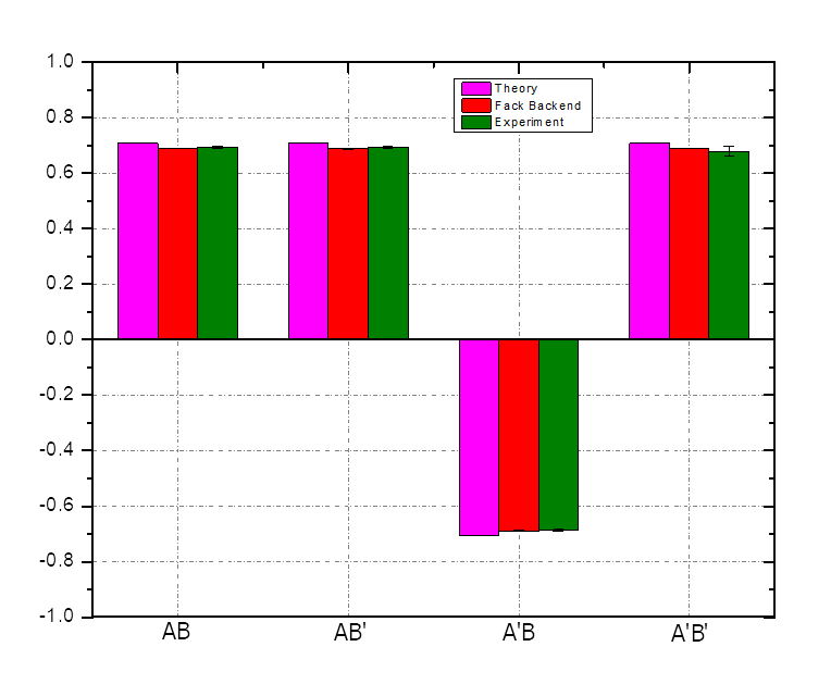
Figure 4: A comparison of the two qubits Bell states theoretically and experimentally obtained expectation values using a fake backend real quantum computer.

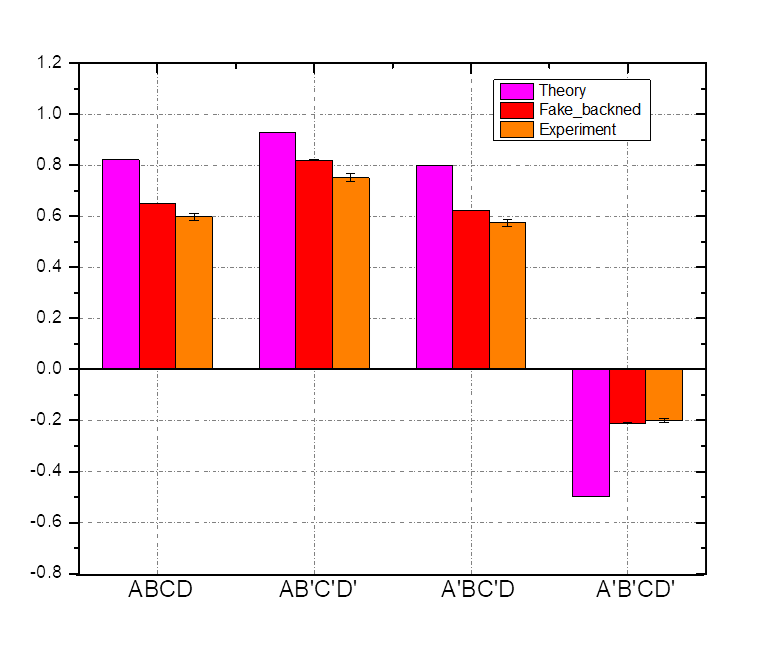
Figure 5: A comparison of the four qubit Dicke state prepared by the gate preparation method theoretically and experimentally obtained expectation values using a fake backend and real quantum computer.

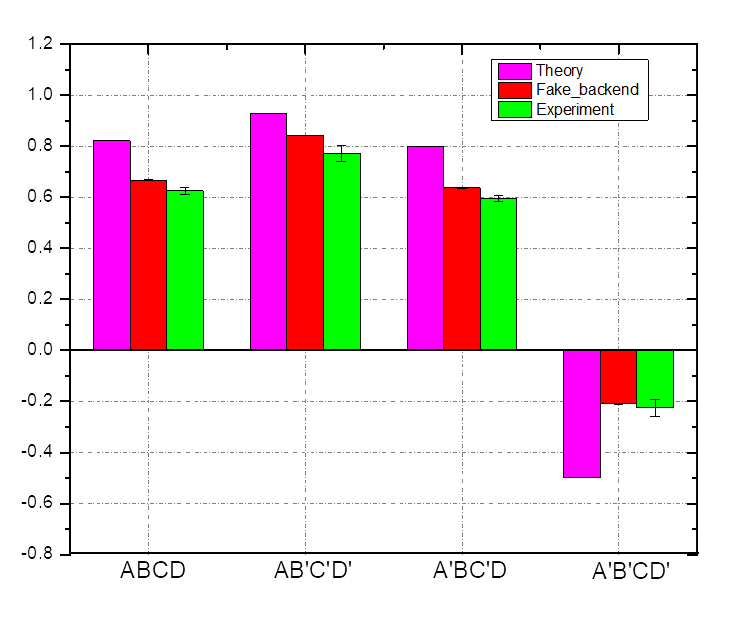
Figure 6: A comparison of the four qubit Dicke state prepared by the state vector method theoretically and experimentally obtained expectation values using a fake backend and real quantum computer and .

For the Bell state, the theoretical maximum violation is 2.82, with the experimental result closely matching at 2.75 on the fake backed and QPU as well. In contrast, for the Dicke state, the theoretical maximum is 3.05, but the experimental value reaches only 2.30 and 2.12 for the gate-based method and 2.35 and 2.21 for the state vector-based method, respectively. This discrepancy can largely be attributed to the deeper circuit depths required for the Dicke state, with depths of 143 and 126, respectively, for Dicke state preparation by gate-based method and state vector-based method, compared to just 9 for the Bell state. The greater depth increases the accumulation of gate and decoherence errors.

Additionally, the Bell state requires only 4 measurements to test its inequality, while the Dicke state involves 40 measurements. Each measurement introduces potential errors, including noise and decoherence, which accumulate across all measurements, contributing significantly to the observed deviation from the theoretical maximum in the Dicke state case.

VI conclusion

In conclusion, we have designed a customized operator that can violate any Bell-type inequalities for any entangled state. Our customized operator is the sum of the identity and Pauli matrices ($I$, $\sigma_{x}$, $\sigma_{y}$, and $\sigma_{z}$). We evaluated the Bell-type violation theoretically and experimentally using the IBM fake backend and QPU for the two-qubit Bell state and four-qubit Dicke state. We obtained the value of CHSH Bell parameter S was $2\sqrt{2}$ theoretically and $2.7534\pm 0.00195$, and $2.7507\pm 0.0197$ experimentally on the fake backend and QPU, respectively, for two-qubit Bell state ($|\Phi^{+}\rangle$) using our customized operator. Using the same approach of the customized operator, we applied it to the four-qubit Dicke state. We have generated the Dicke state using two methods: the gate preparation method and the state vector method. We applied our customized operator to the four-qubit Dicke state for the violation of the Bell-type inequality. We obtained the Bell parameter was $3.05$ theoretically and $2.3030\pm 0.00065$, $2.1239\pm 0.0451$ experimentally on IBM’s fake backend and QPU for gate-based circuit preparation method, respectively and $2.35488\pm 0.00144$, $2.2175\pm 0.0352$ for state vector-based circuit preparation method, which is a clear violation of the local realism for both the methods. The discrepancy between results from fake backends and real quantum hardware arises because fake backends simulate ideal conditions with static, pre-characterized noise models, essentially providing a snapshot of real backend (QPU) errors at a specific time. In contrast, real hardware (QPU) experiences dynamic noise, fluctuations, and decoherence, which leads to higher error rates and less consistent results compared to the simulated environment.

In our investigation, the state vector-based method gives better results as compared to the gate-based method. This could be due to the fact that it initializes the system directly into the desired Dicke state, minimizing the overall circuit depth and noise exposure. By bypassing intermediate gate operations, this approach reduces the likelihood of errors from decoherence and gate imperfections. Even though the gate-based method may use fewer CNOT gates, the statevector method’s combination of lower circuit depth, fewer intermediate operations, and potentially more optimized qubit routing leads to better fidelity on real hardware. We also note that The Bell state shows a close match between theoretical (2.82) and experimental (2.75) violation values due to its lower circuit depth and fewer measurements. In contrast, the Dicke state has a larger discrepancy (theoretical: 3.05, experimental: 2.12 and 2.21) due to significantly higher circuit depth and an increased number of measurements, leading to greater error accumulation. We have successfully shown the violation of the Bell-type inequalities for the two-qubit Bell state and four-qubit Dicke state using our customized operator. In the future, that customized operator can be applied to any Bell-type inequality to any number of entangled states.

Data Availability statement

All data that support the findings of this study are included in the article.

Appendix A Derivation of the Bell polynomial for two-qubit Bell state

Here, we derive the Bell polynomial for the two-qubit Bell state $|\Phi^{+}\rangle$, as described in Eq. (5). Initially, we compute the first term of Eq. (5), as shown in Eq. (III.1). Following a similar approach, we calculate all the remaining terms. Consequently, the Bell polynomial can be expressed as follows:

$$|S_{|\Phi^{+}\rangle}| =\cos(\gamma_{A})[\cos(\gamma_{B})-\cos(\gamma_{B}^{\prime})]+\cos(\gamma_{A}^{\prime})[\cos(\gamma_{B})+\cos(\gamma_{B}^{\prime})]+\cos(\theta_{A})\sin(\gamma_{A})[\cos(\theta_{B})\sin(\gamma_{B})-\cos(\theta_{B}^{\prime})\sin(\gamma_{B}^{\prime})]$$

$$+\cos(\theta_{A}^{\prime})\sin(\gamma_{A}^{\prime})[\cos(\theta_{B})\sin(\gamma_{B})+\cos(\theta_{B}^{\prime})\sin(\gamma_{B}^{\prime})]+\sin(\gamma_{B})\sin(\theta_{B})[\cos(\phi_{A}+\phi_{B})\sin(\gamma_{A})\sin(\theta_{A})$$

$$+\cos(\phi_{A}^{\prime}+\phi_{B})\sin(\gamma_{A}^{\prime})\sin(\theta_{A}^{\prime})]+\sin(\gamma_{B}^{\prime})\sin(\theta_{B}^{\prime})[-\cos(\phi_{A}+\phi_{A}^{\prime})\sin(\gamma_{A})\sin(\theta_{A})$$

$$+\cos(\phi_{A}^{\prime}+\phi_{B}^{\prime})\sin\gamma(\theta_{A})+\cos(\phi_{A}^{\prime}+\cos(\phi_{B}^{\prime})\sin(\theta_{A}^{\prime})].$$ (20)

Appendix B Derivation of the Bell polynomial for four-qubit Dicke state

Here, we took a similar approach as taken for the two-qubit Bell state. Eq. (1) expressed the four qubit Dicke state ($|D^{(2)}_{4}\rangle$), and its Bell-type inequality is defined in Eq. (2). For calculating the Bell polynomial, we first calculate the 1st term in Eq. (2) as follows;

$$\langle\hat{A}\hat{B}\hat{C}\hat{D}\rangle=\langle D^{(2)}_{4}|\bm{\hat{X}_{\hat{n}_{A}}}\otimes\bm{\hat{X}_{\hat{n}_{B}}}\otimes\bm{\hat{X}_{\hat{n}_{C}}}\otimes\bm{\hat{X}_{\hat{n}_{D}}}|D^{(2)}_{4}\rangle\\ =\frac{1}{3}\Bigg{[}\cos(\gamma_{A})\Bigg{(}\sin(\gamma_{B})\Bigg{(}\cos(\gamma_{D})\sin(\gamma_{C})\Big{(}\cos(\theta_{B})\cos(\theta_{C})-2\cos(\phi_{B}-\phi_{C})\sin(\theta_{B})\sin(\theta_{C})\Big{)}+\cos(\gamma_{C})\sin(\gamma_{D})\\ \Big{(}\cos(\theta_{B})\cos(\theta_{D})-2\cos(\phi_{B}-\phi_{D})\sin(\theta_{B})\sin(\theta_{D})\Big{)}\Bigg{)}+\cos(\gamma_{B})\Big{(}3\cos(\gamma_{C})\cos(\gamma_{D})+\sin(\gamma_{C})\sin(\gamma_{D})\Big{(}\cos(\theta_{C})\\ \cos(\theta_{D})-2\cos(\phi_{C}-\phi_{D})\sin(\theta_{C})\sin(\theta_{D})\Big{)}\Big{)}\Bigg{)}+\sin(\gamma_{A})\Bigg{(}\cos(\gamma_{C})\Bigg{(}\cos(\gamma_{D})\sin(\gamma_{B})nonumber\Big{(}\cos(\theta_{A})\cos(\theta_{B})\\ -2\cos(\phi_{A}-\phi_{B})\sin(\theta_{A})\sin(\theta_{B})\Big{)}+\cos(\gamma_{B})\sin(\gamma_{D})\Big{(}\cos(\theta_{A})\cos(\theta_{D})-2\cos(\phi_{A}-\phi_{D})\sin(\theta_{A})\sin(\theta_{D})\Big{)}\Bigg{)}\\ +\sin(\gamma_{C})\Bigg{(}\cos(\gamma_{B})\cos(\gamma_{D})\Big{(}\cos(\theta_{A})\cos(\theta_{C})-2\cos(\phi_{A}-\phi_{C})\sin(\theta_{A})\sin(\theta_{C})\Big{)}+\sin(\gamma_{B})\sin(\gamma_{D})\\ \Bigg{(}\cos(\theta_{D})\Bigg{(}-2\sin(\theta_{A})\Big{(}\cos(\theta_{C})\cos(\phi_{A}-\phi_{B})\sin(\theta_{B})+\cos(\theta_{B})\cos(\phi_{A}-\phi_{C})\sin(\theta_{C})\Big{)}+\cos(\theta_{A})\Big{(}3\cos(\theta_{B})\cos(\theta_{C})\\ -2\cos(\phi_{B}-\phi_{C})\sin(\theta_{B})\sin(\theta_{C})\Big{)}\Bigg{)}+\Big{(}-2\cos(\theta_{B})\Big{(}\cos(\theta_{C})\cos(\phi_{A}-\phi_{D})\sin(\theta_{A})+\cos(\theta_{A})\cos(\phi_{C}-\phi_{D})\sin(\theta_{C})\Big{)}\\ +\sin(\theta_{B})\Big{(}-2\cos(\theta_{A})\cos(\theta_{C})\cos(\phi_{B}-\phi_{D})+\Big{(}\cos(\phi_{A}+\phi_{B}-\phi_{C}-\phi_{D})+2\cos(\phi_{A}-\phi_{B})\cos(\phi_{C}-\phi_{D})\Big{)}\\ \sin(\theta_{A})\sin(\theta_{C})\Big{)}\sin(\theta_{D})\Big{)}\Bigg{)}\Bigg{)}\Bigg{)}\Bigg{]}.$$ (21)

References

- Nielsen and Chuang [2010] M. A. Nielsen and I. L. Chuang, Quantum Computation and Quantum Information: 10th Anniversary Edition (Cambridge University Press, 2010).
- Bennett et al. [1993] C. H. Bennett, G. Brassard, C. Crépeau, R. Jozsa, A. Peres, and W. K. Wootters, Teleporting an unknown quantum state via dual classical and einstein-podolsky-rosen channels, Phys. Rev. Lett. 70, 1895 (1993).
- Bennett and Wiesner [1992] C. H. Bennett and S. J. Wiesner, Communication via one- and two-particle operators on einstein-podolsky-rosen states, Phys. Rev. Lett. 69, 2881 (1992).
- Hillery et al. [1999] M. Hillery, V. Bužek, and A. Berthiaume, Quantum secret sharing, Phys. Rev. A 59, 1829 (1999).
- Gottesman [2000] D. Gottesman, Theory of quantum secret sharing, Phys. Rev. A 61, 042311 (2000).
- Bennett and Brassard [2014] C. H. Bennett and G. Brassard, Quantum cryptography: Public key distribution and coin tossing, Theoretical Computer Science 560, 7 (2014), theoretical Aspects of Quantum Cryptography – celebrating 30 years of BB84.
- Greenberger et al. [1990] D. M. Greenberger, M. A. Horne, A. Shimony, and A. Zeilinger, Bell’s theorem without inequalities, American Journal of Physics 58, 1131 (1990), https://pubs.aip.org/aapt/ajp/article-pdf/58/12/1131/11479397/1131_1_online.pdf .
- Ekert [1991] A. K. Ekert, Quantum cryptography based on bell’s theorem, Phys. Rev. Lett. 67, 661 (1991).
- Scarani and Gisin [2001] V. Scarani and N. Gisin, Quantum communication between partners and bell’s inequalities, Phys. Rev. Lett. 87, 117901 (2001).
- Sen [De] A. Sen(De), U. Sen, and M. Żukowski, Unified criterion for security of secret sharing in terms of violation of bell inequalities, Phys. Rev. A 68, 032309 (2003).
- Brukner et al. [2004] i. c. v. Brukner, M. Żukowski, J.-W. Pan, and A. Zeilinger, Bell’s inequalities and quantum communication complexity, Phys. Rev. Lett. 92, 127901 (2004).
- Pironio et al. [2010] S. Pironio, A. Acín, S. Massar, and et al., Random numbers certified by bell’s theorem, Nature 464, 1021 (2010).
- Clauser et al. [1969a] J. F. Clauser, M. A. Horne, A. Shimony, and R. A. Holt, Proposed experiment to test local hidden-variable theories, Phys. Rev. Lett. 23, 880 (1969a).
- Werner and Wolf [2001] R. F. Werner and M. M. Wolf, All-multipartite bell-correlation inequalities for two dichotomic observables per site, Phys. Rev. A 64, 032112 (2001).
- Weinfurter and Żukowski [2001] H. Weinfurter and M. Żukowski, Four-photon entanglement from down-conversion, Phys. Rev. A 64, 010102 (2001).
- Żukowski and Brukner [2002] M. Żukowski and i. c. v. Brukner, Bell’s theorem for general n-qubit states, Phys. Rev. Lett. 88, 210401 (2002).
- Wu et al. [2009] Y.-C. Wu, P. Badziag, and M. Żukowski, Clauser-horne-shimony-holt-type bell inequalities involving a party with two or three local binary settings, Phys. Rev. A 79, 022110 (2009).
- Mermin [1990] N. D. Mermin, Extreme quantum entanglement in a superposition of macroscopically distinct states, Phys. Rev. Lett. 65, 1838 (1990).
- Ardehali [1992] M. Ardehali, Bell inequalities with a magnitude of violation that grows exponentially with the number of particles, Phys. Rev. A 46, 5375 (1992).
- Belinskiĭ and Klyshko [1993] A. V. Belinskiĭ and D. N. Klyshko, Interference of light and bell’s theorem, Physics-Uspekhi 36, 653 (1993).
- Tura et al. [2014] J. Tura, R. Augusiak, A. B. Sainz, T. Vértesi, M. Lewenstein, and A. Acín, Detecting nonlocality in many-body quantum states, Science 344, 1256 (2014).
- Tura et al. [2015] J. Tura, R. Augusiak, A. B. Sainz, B. Lücke, C. Klempt, M. Lewenstein, and A. Acín, Nonlocality in many-body quantum systems detected with two-body correlators, Annals of Physics 362, 370 (2015).
- Wu et al. [2013] Y.-C. Wu, M. Żukowski, J.-L. Chen, and G.-C. Guo, Compact bell inequalities for multipartite experiments, Phys. Rev. A 88, 022126 (2013).
- Dicke [1954] R. H. Dicke, Coherence in spontaneous radiation processes, Phys. Rev. 93, 99 (1954).
- Kiesel et al. [2007] N. Kiesel, C. Schmid, G. Tóth, E. Solano, and H. Weinfurter, Experimental observation of four-photon entangled dicke state with high fidelity, Phys. Rev. Lett. 98, 063604 (2007).
- Krischek et al. [2011] R. Krischek, C. Schwemmer, W. Wieczorek, H. Weinfurter, P. Hyllus, L. Pezzé, and A. Smerzi, Useful multiparticle entanglement and sub-shot-noise sensitivity in experimental phase estimation, Phys. Rev. Lett. 107, 080504 (2011).
- Hyllus et al. [2012] P. Hyllus, W. Laskowski, R. Krischek, C. Schwemmer, W. Wieczorek, H. Weinfurter, L. Pezzé, and A. Smerzi, Fisher information and multiparticle entanglement, Phys. Rev. A 85, 022321 (2012).
- Duan [2011] L.-M. Duan, Entanglement detection in the vicinity of arbitrary dicke states, Phys. Rev. Lett. 107, 180502 (2011).
- Zhao et al. [2015] Y.-Y. Zhao, Y.-C. Wu, G.-Y. Xiang, C.-F. Li, and G.-C. Guo, Experimental violation of the local realism for four-qubit dicke state, Opt. Express 23, 30491 (2015).
- Wieczorek et al. [2009] W. Wieczorek, R. Krischek, N. Kiesel, P. Michelberger, G. Tóth, and H. Weinfurter, Experimental entanglement of a six-photon symmetric dicke state, Phys. Rev. Lett. 103, 020504 (2009).
- Prevedel et al. [2009] R. Prevedel, G. Cronenberg, M. S. Tame, M. Paternostro, P. Walther, M. S. Kim, and A. Zeilinger, Experimental realization of dicke states of up to six qubits for multiparty quantum networking, Phys. Rev. Lett. 103, 020503 (2009).
- Wieczorek et al. [2008] W. Wieczorek, C. Schmid, N. Kiesel, R. Pohlner, O. Gühne, and H. Weinfurter, Experimental observation of an entire family of four-photon entangled states, Phys. Rev. Lett. 101, 010503 (2008).
- Schmid et al. [2008] C. Schmid, N. Kiesel, W. Laskowski, W. Wieczorek, M. Żukowski, and H. Weinfurter, Discriminating multipartite entangled states, Phys. Rev. Lett. 100, 200407 (2008).
- Emilio Pelaez and Sosa [2022] P. S. C. Emilio Pelaez, Anuranan Das and D. S. Sosa arXiv:2203.12943v2 (2022).
- Malik et al. [2019] G. Malik, R. Singh, B. Behera, and P. Panigrahi, First experimental demonstration of multi-particle quan-tum tunneling in ibm quantum computer, (2019).
- Halder et al. [2018] K. Halder, N. N. Hegade, B. K. Behera, and P. K. Panigrahi, Digital quantum simulation of laser-pulse induced tunneling mechanism in chemical isomerization reaction., arXiv: Quantum Physics (2018).
- García-Martín and Sierra [2018] D. García-Martín and G. Sierra, Five experimental tests on the 5-qubit ibm quantum computer, Journal of Applied Mathematics and Physics 6, 1460 (2018).
- Alsina and Latorre [2016] D. Alsina and J. I. Latorre, Experimental test of mermin inequalities on a five-qubit quantum computer, Phys. Rev. A 94, 012314 (2016).
- Majumder et al. [2017] A. Majumder, S. Mohapatra, and A. Kumar, Experimental realization of secure multiparty quantum summation using five-qubit ibm quantum computer on cloud 10.48550/arxiv.1707.07460 (2017).
- Roffe et al. [2018] J. Roffe, D. Headley, N. Chancellor, D. Horsman, and V. Kendon, Protecting quantum memories using coherent parity check codes, Quantum Science and Technology 3, 035010 (2018).
- Mahanti et al. [2019] S. Mahanti, S. Das, B. K. Behera, and P. K. Panigrahi, Quantum robots can fly; play games: an IBM quantum experience, Quantum Inf. Process. 18, 219 (2019).
- Crow and Joynt [2014] D. Crow and R. Joynt, Classical simulation of quantum dephasing and depolarizing noise, Phys. Rev. A 89, 042123 (2014).
- Mukherjee et al. [2020] C. S. Mukherjee, S. Maitra, V. Gaurav, and D. Roy, Preparing dicke states on a quantum computer, IEEE Transactions on Quantum Engineering 1, 1 (2020).
- Iten et al. [2016] R. Iten, R. Colbeck, I. Kukuljan, J. Home, and M. Christandl, Quantum circuits for isometries, Phys. Rev. A 93, 032318 (2016).
- Clauser et al. [1969b] J. F. Clauser, M. A. Horne, A. Shimony, and R. A. Holt, Proposed experiment to test local hidden-variable theories, Phys. Rev. Lett. 23, 880 (1969b).
- Javadi-Abhari et al. [2024] A. Javadi-Abhari, M. Treinish, K. Krsulich, C. J. Wood, J. Lishman, J. Gacon, S. Martiel, P. D. Nation, L. S. Bishop, A. W. Cross, B. R. Johnson, and J. M. Gambetta, Quantum computing with Qiskit (2024), arXiv:2405.08810 [quant-ph] .
- Nation et al. [2021] P. D. Nation, H. Kang, N. Sundaresan, and J. M. Gambetta, Scalable mitigation of measurement errors on quantum computers, PRX Quantum 2, 040326 (2021).