Abstract

In this study, we explore an ensemble-based approach to improve classification accuracy in complex image datasets. Utilizing a Convolutional Block Attention Module (CBAM) alongside a Deep Neural Network (DNN) we leverage the unique feature-extraction capabilities of each model to enhance the overall accuracy. Additional models, such as Random Forest, XGBoost, Support Vector Machine (SVM), and K-Nearest Neighbors (KNN), are introduced to further diversify the predictive power of our ensemble. By leveraging these methods, the proposed approach provides robust feature discrimination and improved classification results. Experimental evaluations demonstrate that the ensemble achieves higher accuracy and robustness across challenging and imbalanced classes, showing significant promise for broader applications in computer vision tasks.

Keywords: Attention, Ensemble, Latent Space, Autoencoder, Support Vector Machine (SVM), K-Nearest Neighbors (KNN), Deep Neural Network (DNN)

1 Introduction

Image classification is a critical task within computer vision, particularly in medical imaging applications such as capsule endoscopy, where accurate diagnosis can significantly impact patient outcomes [1]. During capsule endoscopy, a patient ingests a small capsule containing a camera that captures thousands of images of the gastrointestinal tract, necessitating precise interpretation of these images to identify abnormalities. Traditional diagnostic processes often rely on expert interpretation of these images, which can be subject to human error and variability. Studies indicate that approximately 20% of diagnostic errors can be attributed to incorrect interpretation of imaging data, leading to delayed or inappropriate treatment. Moreover, the increasing volume of medical data poses a challenge for clinicians, emphasizing the need for automated systems that enhance diagnostic precision and efficiency [2].

Recent advancements in deep learning, particularly in ensemble methods and attention mechanisms, have demonstrated potential for improving classification accuracy by harnessing the strengths of multiple models. In the context of capsule endoscopy, where a large number of images are captured, automation in image diagnosis not only streamlines the workflow but also facilitates quicker decision-making. This enables healthcare professionals to concentrate on patient care rather than being burdened by time-consuming analysis [3].

This paper presents an ensemble approach incorporating several machine learning models to achieve robust feature extraction and optimized decision-making for classification tasks. The primary aim of this research is to integrate the feature-selective capabilities of established classifiers to make the final classification decision. Through systematic experiments, we evaluate the effectiveness of our ensemble in handling complex datasets with varying class distributions, demonstrating its potential application across a range of challenging scenarios, particularly in the realm of capsule endoscopy [4].

2 Methods

2.1 Data Augmentation

The dataset used in this study comprises high-resolution images spanning ten distinct classes, each representing a specific abnormality or a healthy control. Each image in the dataset has been preprocessed to a uniform resolution of 224x224 pixels.

Given the class imbalance within the dataset, with a predominant representation of the “Normal” class and significantly fewer samples for rarer abnormalities like “Worms” and “Ulcer” data augmentation was essential to generate sufficient samples for all classes. The target was to increase the dataset size to a minimum of 7,500 images per class, ensuring that each abnormality is well-represented in training. The augmentation [5] process utilized the multiple transformations, with specific design choices to retain medical relevancy and variability. Random horizontal and vertical flips were applied to enhance the model’s ability to recognize abnormalities regardless of left-right or top-bottom orientation, a common challenge in gastrointestinal imaging. Random rotations within ±20 degrees were used to mimic different orientations of the gastrointestinal tract within the capsule’s viewpoint, as this varies during patient examination. We included both zoom-in and zoom-out transformations, with scaling factors of ±15%. Zoom-in transformations simulate a closer inspection of mucosal abnormalities, while zoom-out provides a broader context. Using shearing up to ±10°, elastic transformations or shearing simulate slight distortions in the capsule camera’s viewpoint, an effect seen due to natural movement and tract curvature. Gaussian blur transformation, applied with a kernel size of 5 and sigma between 0.1 and 1.0, was used to account for minor blurring in capsule images due to motion artifacts. By randomly cropping between 85-100% of the original image and resizing it back to 224x224 pixels, this transformation introduces spatial variety without altering the underlying anatomy of the abnormality. Gaussian noise [6] with a standard deviation of 0.05 was added to simulate real-world sensor noise, improving the model’s resilience to slight pixel-level variations. We also used Image Sharpening, as Enhancing the edges and details could improve the model’s focus on fine structures within the gastrointestinal images.

Class	Training	Validation	Training Examples
	Examples	Examples	(After Augmentation)
Angioectasia	1,154	497	7,500
Bleeding	834	359	7,500
Erosion	2,694	1,155	7,500
Erythema	691	297	7,500
Foreign Body	792	340	7,500
Lymphangiectasia	796	343	7,500
Normal	28,663	12,287	28,663
Polyp	1,162	500	7,500
Ulcer	663	286	7,500
Worms	158	68	7,500
Total	37,607	16,132	96,163

Table 1: Overview of the dataset’s original and post- augmentation instance counts and their division among classes

The augmentation process was implemented with additional custom functions for Gaussian noise and conditional transformation application. Each class directory within the training set was iterated over. For classes with fewer than 7,500 samples, random transformations were applied in batches to achieve the target sample size. The dataset distribution before augmentation is shown in table 1. The augmentation workflow consisted of randomly selecting between 2 and 4 transformations per image, ensuring variability while preserving anatomical features. We avoided brightness and color augmentations, as capsule endoscopy operates under controlled lighting conditions, and such features are crucial for detecting certain abnormalities.

2.2 Autoencoder with ResNet

An autoencoder architecture based on ResNet50 [7] was developed to extract feature representations from images and to generate reconstructed images. The autoencoder consists of two main components: an encoder and a decoder.

ResNet Architecture: The encoder utilizes a ResNet50 backbone, pre-trained on ImageNet, which is a deep residual network that facilitates the training of very deep networks through skip connections (or residual connections). The ResNet50 architecture includes 50 layers, comprising convolutional layers, batch normalization layers, ReLU activations, and skip connections, allowing the model to learn identity mappings. The architecture can be summarized as follows:

$$ResNet(x)=F(x)+x$$ (1)

where $F(x)$ represents the convolutional operation, and $x$ is the input to the residual block, as shown in eq. 1. This structure promotes efficient training and better gradient flow, which is particularly advantageous when learning from complex image datasets.

The ResNet encoder processes the input images $I$ and generates a latent representation $z$ as follows:

$$z=Encoder(I)\in\mathbb{R}^{1024}$$ (2)

As shown in eq. 2, the final fully connected layer of ResNet was replaced with a linear layer, which outputs a latent space representation of size 1024.

The decoder takes the latent representation $z$ and reconstructs the original image $\hat{I}$:

$$\hat{I}=Decoder(z)$$ (3)

The decoding process, as described in eq. 3, comprises several transposed convolutional layers, which progressively upscale the latent representation back to the original image dimensions. The reconstruction is evaluated using Mean Squared Error (MSE) loss, defined as:

$$Loss=\frac{1}{N}\sum_{i=1}^{N}(I_{i}-\hat{I}_{i})^{2}$$ (4)

where $N$ represents the number of pixels in the image, as shown in eq. 4. The model was trained over a set number of epochs, adjusting the weights via the Adam optimizer to minimize the reconstruction loss.

Upon completion of training, the reconstructed images generated by the autoencoder were merged back into the training dataset. This integration aims to enhance the diversity of the training data, effectively increasing the dataset size and aiding subsequent classification tasks. The latent space representations $z$ generated from the validation set during the encoding process will be stored and utilized for training multiple models in later stages of the project. The final latent space representations are expected to contain condensed, relevant information about the input images, making them suitable for further model training tasks, including classification and anomaly detection.

2.3 Syn-XRF Model

In this study, we implemented an ensemble model consisting of four distinct classifiers: Support Vector Machine (SVM) [8], Random Forest [9], K-Nearest Neighbors (KNN) [10], and XGBoost [11]. Each classifier was employed to generate probabilistic outputs for class labels based on their respective learning mechanisms.

The Support Vector Machine was utilized to find the optimal hyperplane that separates the classes in the latent space representations. The decision function of SVM can be mathematically expressed as shown in eq. 5.

$$f(x)=w^{T}x+b$$ (5)

where $w$, $x$, and $b$ represent the weight vector, input feature vector, and the bias term, respectively. The optimization goal is to maximize the margin between the classes, as depicted in eq. 6.

$$\text{maximize }\frac{2}{||w||}\quad\text{subject to }y_{i}(w^{T}x_{i}+b)\geq 1\text{ for all }i$$ (6)

The Random Forest [12] ensemble method constructs multiple decision trees during training and outputs the mode of the classes (classification) or mean prediction (regression) of the individual trees. The final class prediction can be represented as in eq. 7.

$$\hat{y}=\text{mode}(h_{1}(x),h_{2}(x),\dots,h_{n}(x))$$ (7)

where $h_{i}(x)$ represents the decision of the $i$-th decision tree.

KNN [13] classifies instances based on the majority label of their $k$ nearest neighbors in the feature space. The predicted label $\hat{y}$ for a sample $x$ can be represented as in eq. 8.

$$\hat{y}=\text{argmax}_{j}\sum_{i=1}^{k}I(y_{i}=j)$$ (8)

where $I$ is the indicator function that returns 1 if the class label $y_{i}$ equals $j$ and 0 otherwise.

XGBoost [14] applies gradient boosting techniques to enhance classification precision. The model combines multiple weak learners (typically decision trees) to form a strong learner. The final prediction for a sample can be expressed as in eq. 9.

$$\hat{y}=\sum_{i=1}^{N}\alpha_{i}h_{i}(x)$$ (9)

where $h_{i}(x)$ represents the output of the $i$-th tree and $\alpha_{i}$ is the weight associated with that tree.

The ensemble model aggregates the predictions from the aforementioned classifiers using a voting mechanism. In our implementation, we utilized soft voting, which considers the predicted probabilities of each class for each classifier. The final prediction can be mathematically described as shown in eq. 10.

$$\hat{y}=\text{argmax}_{j}\sum_{i=1}^{M}P(h_{i}(x)=j),\quad\text{for }j\in\text{Classes}$$ (10)

In this approach, each classifier contributes its unique strengths. The Random Forest model excels in handling high-dimensional data and mitigating overfitting by aggregating the results of multiple decision trees, providing robustness against noise. XGBoost leverages gradient boosting, allowing for efficient handling of missing values and the incorporation of complex patterns through its tree-boosting framework, thus enhancing predictive accuracy. The Support Vector Machine (SVM) is adept at finding optimal hyperplanes in high-dimensional spaces, making it effective for margin-based classification, particularly in cases with clear class separations. Lastly, K-Nearest Neighbors (KNN) offers simplicity and adaptability, providing intuitive classifications based on proximity in feature space, which is particularly useful for capturing local structures. By combining these classifiers, we aim to harness their diverse strengths, leading to improved overall performance in classification tasks. The combination of diverse classifiers within the ensemble effectively enhances the model’s predictive performance on the validation set.

2.4 CBAM-Enhanced ResNet Architecture

We have implemented the Convolutional Block Attention Module (CBAM [15] [16]) to enhance the feature extraction capabilities of our classification model. The CBAM is designed to focus on significant features by applying attention mechanisms across both spatial and channel dimensions, thereby improving the model’s performance in distinguishing between different classes. The architecture of the CBAM consists of two primary components - the Spatial Attention Module and the Channel Attention Module.

• Spatial Attention Module (SAM) operates by generating a spatial attention map that highlights important regions in the feature map. Given an input feature map $F\in\mathbb{R}^{C\times H\times W}$ (where $C$ represents the number of channels, $H$ the height, and $W$ the width), the SAM computes a spatial attention map $M_{s}$, as shown in eq. 11.

  $$M_{s}=\sigma(\text{Conv}(\text{concat}(\text{max}(F),\text{avg}(F))))\cdot F$$ (11)

  where $\sigma$ is the sigmoid activation function, Conv represents a convolution operation, and max and avg denote the maximum and average pooling operations across the channel dimension, respectively. The concatenated feature maps are processed through a convolutional layer to yield the final attention map.

• Channel Attention Module (CAM) emphasizes the importance of various channels by learning a channel attention vector. For a given input $F$, the channel attention map $M_{c}$ is generated using eq. 12.

  $$M_{c}=\sigma(W_{2}\cdot\text{ReLU}(W_{1}\cdot\text{GlobalAvgPool}(F)))$$ (12)

  Here, $W_{1}$ and $W_{2}$ are weight matrices of learnable parameters in the linear layers, and GlobalAvgPool is the global average pooling operation applied to the input feature map $F$. The output of the CAM is then multiplied by the original feature map $F$ to enhance its discriminative power. The combined output from both modules is expressed as eq. 13.

$$F^{\prime}=M_{c}\cdot(M_{s}\cdot F)$$ (13)

where $F^{\prime}$ represents the refined feature map after applying both attention mechanisms. This refined feature map is then fed into the subsequent layers of the model for classification.

The architecture of the CBAM-Enhanced ResNet model utilizes ResNet-18 as its backbone, which consists of several convolutional layers and residual blocks designed to capture hierarchical features effectively. The CBAM is applied to the output of the final feature extraction layer of the ResNet. Specifically, the attention mechanism focuses on enhancing critical feature maps before they are passed to the fully connected layer. A linear layer follows the CBAM to perform classification based on the refined feature maps, yielding predictions across classes.

This model was employed for its ability to enhance feature representation through spatial and channel attention mechanisms. This dual attention allows the model to focus on relevant features while minimizing the impact of less informative ones, which is crucial for image classification tasks. By improving sensitivity to salient features, CBAM enhances classification accuracy and model interpretability, making it particularly beneficial in complex medical imaging scenarios where subtle distinctions between classes are critical for accurate diagnosis.

2.5 Deep Neural Network

Aside from the previously discussed CBAM and ensemble model, a Deep Neural Network (DNN) [17] was designed and implemented to perform classification tasks based on features extracted from a pre-trained autoencoder. The architecture of the DNN consists of multiple fully connected layers, which transform the latent representations into class probabilities, thereby enhancing the model’s ability to differentiate between various image classes.

The DNN is constructed by utilizing a feature extractor based on the ResNet50 architecture, which has been modified to exclude the fully connected layer, enabling it to produce a latent representation of size $L$, where $L=1024$. This modification allows for the reduction of dimensionality while maintaining the essential information required for classification. The latent representation $z$ is derived from the input image $x$, as shown in eq. 14.

$$z=f_{\text{encoder}}(x)=W_{\text{encoder}}\cdot x+b_{\text{encoder}}$$ (14)

where $W_{\text{encoder}}$ and $b_{\text{encoder}}$ represent the weights and biases of the encoder, respectively.

The subsequent fully connected layers of the DNN can be represented by the following equations, where each layer applies a linear transformation followed by a non-linear activation function (ReLU) and, in some cases, dropout for regularization, as shown in eqs. 15, 16, 17, 18, 19, 20 and 21.

1. First Layer:

   $$h_{1}=\text{ReLU}(W_{1}\cdot z+b_{1})$$ (15)

2. Second Layer:

   $$h_{2}=\text{ReLU}(W_{2}\cdot h_{1}+b_{2})$$ (16)

3. Dropout Layer (applied after the second layer):

   $$h_{2}^{\prime}=\text{Dropout}(h_{2})$$ (17)

4. Third Layer:

   $$h_{3}=\text{ReLU}(W_{3}\cdot h_{2}^{\prime}+b_{3})$$ (18)

5. Fourth Layer:

   $$h_{4}=\text{ReLU}(W_{4}\cdot h_{3}+b_{4})$$ (19)

6. Dropout Layer (applied after the fourth layer):

   $$h_{4}^{\prime}=\text{Dropout}(h_{4})$$ (20)

7. Final Output Layer:

   $$y=W_{\text{output}}\cdot h_{4}^{\prime}+b_{\text{output}}$$ (21)

Here, $W_{i}$ and $b_{i}$ represent the weights and biases of the $i$-th layer, and $y$ is the output vector containing class scores. The output of the DNN is processed using the softmax function to yield class probabilities $P(y_{i}\mid x)$, as shown in eq. 22.

$$P(y_{i}\mid x)=\frac{e^{y_{i}}}{\sum_{j=1}^{C}e^{y_{j}}}$$ (22)

where $C$ is the total number of classes. The model is trained to minimize the cross-entropy loss defined as indicated in eq. 23.

$$L=-\frac{1}{N}\sum_{i=1}^{N}\sum_{c=1}^{C}y_{ic}\log(P(y_{c}\mid x_{i}))$$ (23)

where $N$ is the number of training samples, and $y_{ic}$ is a binary indicator (0 or 1) of whether class label $c$ is the correct classification for observation $i$.

The model was trained over 50 epochs with a batch size of 32, employing the Adam optimizer with a learning rate of 0.001. The training process iteratively updated the weights to minimize the loss function while evaluating the model’s performance on a validation dataset. The training and validation accuracy were calculated to monitor the model’s learning progress. The detailed training procedure involved iterative updates based on gradients derived from the loss function, ultimately enabling the DNN to effectively classify the given images based on the learned latent representations.

The Deep Neural Network (DNN) was appropriate for this classification task due to its ability to learn complex feature representations from high-dimensional image data. DNNs can model non-linear decision boundaries, making them effective for distinguishing between classes that are not linearly separable. By utilizing latent space features extracted from the autoencoder, the DNN refines these high-level representations for improved classification accuracy. Furthermore, the architecture allows for high-capacity learning, which, when combined with regularization techniques like dropout, enhances generalization and robustness against overfitting. Collectively, these attributes make DNNs well-suited for tackling complex image classification challenges.

2.6 CAVE-Net

The final classification was determined using a soft voting mechanism [18], where the predicted probabilities from the three separate models—CBAM, DNN, the ensemble model—contributed to the ultimate decision, as depicted in Figure 1. Each model was executed in parallel, enabling simultaneous computation of their respective output probabilities. The Convolutional Block Attention Module (CBAM) was employed for its ability to enhance feature representation by focusing on both spatial and channel dimensions, thereby improving the model’s sensitivity to important features in the images. The Deep Neural Network (DNN) was utilized due to its capacity to learn complex non-linear relationships within the extracted latent features, enabling effective classification through multiple fully connected layers. The third model, an additional ensemble approach, was incorporated to leverage a different learning paradigm, thereby broadening the ensemble’s ability to capture diverse patterns in the data.

By combining the outputs of these three models through soft voting, we aimed to harness their individual strengths and mitigate their respective weaknesses. This synergistic approach allows the ensemble to benefit from the nuanced feature extraction capabilities of CBAM, the deep learning power of DNN, and the complementary insights provided by the third model. The soft voting strategy aggregates the predicted probabilities for each class, selecting the class with the highest cumulative probability as the final output. This method not only enhances classification accuracy but also increases robustness against overfitting and biases inherent to individual models, resulting in improved overall performance in the complex task of image classification.

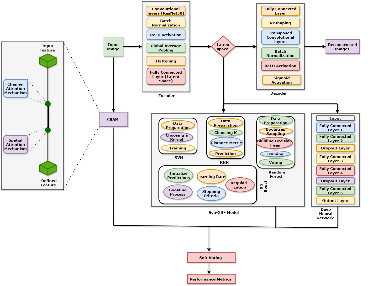
Figure 1: Architecture of proposed framework, CAVE-Net

3 Results

3.1 Experimental Setup

The model has been trained and tested with Python 3.10 on Ubuntu 20.04.6 LTS, using 251.5 GB of memory, an Intel Xeon Silver 4210R CPU (40 cores), and a 25GB NVIDIA RTX A5000 GPU. The model was trained on augmented images and evaluated on validation data from CVIP.

3.2 Achieved results on the validation dataset

The model achieved an overall accuracy of 91.24% on the CVIP 2024 Validation Dataset. The detailed metrics are displayed in table 2.

Model	Accuracy	Precision	Recall	F1 Score
XGB	0.8336	0.8314	0.6854	0.7358
SVM	0.8599	0.8101	0.7391	0.7991
Syn- XRF	0.8704	0.8644	0.8732	0.8623
CBAM	0.9009	0.9033	0.9009	0.9020
CAVE-Net	0.9124	0.9203	0.9198	0.9200

Table 2: Comparison of CAVE-Net Performance Metrics

4 Discussion

Our study demonstrates that the ensemble approach integrating CBAM, DNN and traditional machine learning models significantly enhances classification performance in multi-class abnormality detection, particularly in medical imaging. The CBAM module effectively highlights critical features, improving the model’s ability to detect subtle but significant differences indicative of specific conditions. The DNN architecture complements this by learning complex patterns, while traditional models like Random Forest, XGBoost, SVM and KNN manage issues such as overfitting and class imbalance. Their combination for final classification boosts accuracy, leveraging the strengths of each model to create a reliable framework. Compared to simpler approaches like Logistic Regression or Decision Trees, our ensemble is more appropriate for handling high-dimensional and variable-quality data, representing a significant advancement in automated diagnosis. This approach has the potential to greatly enhance medical diagnostics by reducing diagnostic errors and expediting patient care. Continued refinement of this model can lead to even greater precision in automated diagnosis, and significantly benefit the medical field.

5 Conclusion

We have used a combination of Convolutional Block Attention Module,Deep Neural Network, and ensemble techniques such as Random Forest, XGBoost, SVM and KNN. This combination effectively leverages the strengths of each individual model, resulting in enhanced accuracy and robustness in classification tasks. The synergy created by this ensemble approach demonstrates its superiority over the other frameworks examined, underscoring its potential for practical applications in automated diagnosis.

6 Acknowledgments

As participants in the Capsule Vision 2024 Challenge, we fully comply with the competition’s rules as outlined in [19]. Our AI model development is based exclusively on the datasets provided in the official release in [20]. Additionally, we would like to extend their gratitude to the Centre of Excellence (CoE) in Artificial Intelligence (AI) of Netaji Subhas University of Technology (NSUT), New Delhi, for providing the resources and support needed for this research.

References

- Srivastava et al. [2024] A. Srivastava, N. K. Tomar, U. Bagci, and D. Jha. Video capsule endoscopy classification using focal modulation guided convolutional neural network. Journal Name, 2024.
- Jha et al. [2021] D. Jha, S. Ali, S. Hicks, V. Thambawita, H. Borgli, P. H. Smedsrud, T. de Lange, K. Pogorelov, X. Wang, and P. Harzig. A comprehensive analysis of classification methods in gastrointestinal endoscopy imaging. Medical Image Analysis, 70:102007, 2021.
- Iddan et al. [2000] G. Iddan, G. Meron, A. Glukhovsky, and P. Swain. Wireless capsule endoscopy. Nature, 405(6785):417, 2000.
- Smedsrud et al. [2021] P. H. Smedsrud, V. Thambawita, S. A. Hicks, H. Gjestang, O. O. Nedrejord, E. Næss, H. Borgli, D. Jha, T. J. D. Berstad, and S. L. Eskeland. Kvasir-capsule, a video capsule endoscopy dataset. Scientific Data, 8(1):1–10, 2021.
- Yang et al. [2023] Suorong Yang, Weikang Xiao, Mengchen Zhang, Suhan Guo, Jian Zhao, and Furao Shen. Image data augmentation for deep learning: A survey, 2023. URL https://arxiv.org/abs/2204.08610.
- Taniguchi and Furuta [2024] Takara Taniguchi and Ryosuke Furuta. Learning gaussian data augmentation in feature space for one-shot object detection in manga, 2024. URL https://arxiv.org/abs/2410.05935.
- He et al. [2015] Kaiming He, Xiangyu Zhang, Shaoqing Ren, and Jian Sun. Deep residual learning for image recognition, 2015. URL https://arxiv.org/abs/1512.03385.
- Hearst et al. [1998] M.A. Hearst, S.T. Dumais, E. Osuna, J. Platt, and B. Scholkopf. Support vector machines. IEEE Intelligent Systems and their Applications, 13(4):18–28, 1998. doi: 10.1109/5254.708428.
- Breiman [2001] Leo Breiman. Random forests. Machine learning, 45:5–32, 2001.
- Laaksonen and Oja [1996] Jorma Laaksonen and Erkki Oja. Classification with learning k-nearest neighbors. In Proceedings of international conference on neural networks (ICNN’96), volume 3, pages 1480–1483. IEEE, 1996.
- Chen and Guestrin [2016a] Tianqi Chen and Carlos Guestrin. Xgboost: A scalable tree boosting system. In Proceedings of the 22nd acm sigkdd international conference on knowledge discovery and data mining, pages 785–794, 2016a.
- Surve and Pradhan [2024] Tanmay Surve and Romila Pradhan. Example-based explanations for random forests using machine unlearning, 2024. URL https://arxiv.org/abs/2402.05007.
- Cunningham and Delany [2021] Pádraig Cunningham and Sarah Jane Delany. k-nearest neighbour classifiers - a tutorial. ACM Computing Surveys, 54(6):1–25, July 2021. ISSN 1557-7341. doi: 10.1145/3459665. URL http://dx.doi.org/10.1145/3459665.
- Chen and Guestrin [2016b] Tianqi Chen and Carlos Guestrin. Xgboost: A scalable tree boosting system. In Proceedings of the 22nd ACM SIGKDD International Conference on Knowledge Discovery and Data Mining, volume 11 of KDD ’16, page 785–794. ACM, August 2016b. doi: 10.1145/2939672.2939785. URL http://dx.doi.org/10.1145/2939672.2939785.
- Woo et al. [2018a] Sanghyun Woo, Jongchan Park, Joon-Young Lee, and In So Kweon. Cbam: Convolutional block attention module, 2018a. URL https://arxiv.org/abs/1807.06521.
- Woo et al. [2018b] Sanghyun Woo, Jongchan Park, Joon-Young Lee, and In So Kweon. Cbam: Convolutional block attention module. In Proceedings of the European conference on computer vision (ECCV), pages 3–19, 2018b.
- Schmidhuber [2015] Jürgen Schmidhuber. Deep learning in neural networks: An overview. Neural Networks, 61:85–117, January 2015. ISSN 0893-6080. doi: 10.1016/j.neunet.2014.09.003. URL http://dx.doi.org/10.1016/j.neunet.2014.09.003.
- Gu and Meng [2024] Renhua Gu and Xiangfeng Meng. Aispace at semeval-2024 task 8: A class-balanced soft-voting system for detecting multi-generator machine-generated text, 2024. URL https://arxiv.org/abs/2404.00950.
- Handa et al. [2024a] Palak Handa, Amirreza Mahbod, Florian Schwarzhans, Ramona Woitek, Nidhi Goel, Deepti Chhabra, Shreshtha Jha, Manas Dhir, Deepak Gunjan, Jagadeesh Kakarla, et al. Capsule vision 2024 challenge: Multi-class abnormality classification for video capsule endoscopy. arXiv preprint arXiv:2408.04940, 2024a.
- Handa et al. [2024b] Palak Handa, Amirreza Mahbod, Florian Schwarzhans, Ramona Woitek, Nidhi Goel, Deepti Chhabra, Shreshtha Jha, Manas Dhir, Deepak Gunjan, Jagadeesh Kakarla, and Balasubramanian Raman. Training and Validation Dataset of Capsule Vision 2024 Challenge. Fishare, 7 2024b. doi: 10.6084/m9.figshare.26403469.v1. URL https://figshare.com/articles/dataset/Training_and_Validation_Dataset _of_Capsule_Vision_2024_Challenge/26403469.