Causality-Respecting Adaptive Refinement for PINNs: Enabling Precise Interface Evolution in Phase Field Modeling

Abstract

Physics-informed neural networks (PINNs) have emerged as a powerful tool for solving physical systems described by partial differential equations (PDEs). However, their accuracy in dynamical systems, particularly those involving sharp moving boundaries with complex initial morphologies, remains a challenge. This study introduces an approach combining residual-based adaptive refinement (RBAR) with causality-informed training to enhance the performance of PINNs in solving spatio-temporal PDEs. Our method employs a three-step iterative process: initial causality-based training, RBAR-guided domain refinement, and subsequent causality training on the refined mesh. Applied to the Allen-Cahn equation, a widely-used model in phase field simulations, our approach demonstrates significant improvements in solution accuracy and computational efficiency over traditional PINNs. Notably, we observe an ’overshoot and relocate’ phenomenon in dynamic cases with complex morphologies, showcasing the method’s adaptive error correction capabilities. This synergistic interaction between RBAR and causality training enables accurate capture of interface evolution, even in challenging scenarios where traditional PINNs fail. Our framework not only resolves the limitations of uniform refinement strategies but also provides a generalizable methodology for solving a broad range of spatio-temporal PDEs. The simplicity and effectiveness of our RBAR-causality combined PINN offer promising potential for applications across various physical systems characterized by complex, evolving interfaces.

1 Introduction

Partial differential equations (PDEs) are fundamental in science and engineering, modeling phenomena from fluid flow to material failure. While analytical solutions are limited, numerical methods have been the primary approach for solving PDEs. Traditional physics-based numerical methods like finite element, isogeometric analysis, and spectral methods offer high accuracy but can be computationally expensive. In recent years, deep learning (DL) has emerged as a promising alternative for fast predictions of physical systems.

Within the broader category of DL techniques, physics-informed neural networks (PINNs) [1, 2] have gained particular attention as an alternative to traditional PDE solvers. PINNs approximate PDE solutions by training a deep neural network (DNN) to minimize a loss function that incorporates initial and boundary conditions, as well as the PDE residual at selected points (collocation points). This approach is essentially a mesh-free technique that converts the problem of directly solving governing equations into a loss function optimization problem. PINNs integrate the mathematical model into the network without requiring labeled data, reinforcing the loss function with a residual term from the governing equation that acts as a penalizing term, thus ensuring the network considers the underlying physics rather than solely fitting data. Numerous variants of PINNs have been developed including conservative PINNs [3], sparse PINNs [4], varitaional PINNs [5], domain-decomposition PINNs (XPINNs) [6], and separable PINNs [7], stochastic PINNs [8] to name a few. However, PINNs are not the only methods that constrain ML models with physics. Other popular methods that use DNNs to solve PDEs include the Deep Ritz method [9] and approaches based on the Galerkin or Petrov-Galerkin method [10] including the Deep Galerkin Method [11]. When a Galerkin approach is used on collocation points, the framework is a variant of PINNs, i.e. hp-VPINNs [10]. In the Deep Energy Method [2] the loss function minimizes the variational energy of the system at quadrature points. Other methods have used GPs to solve PDEs [12, 13] or have imposed physical constraints on GPs [14].

While PINNs have demonstrated success across various domains, their application to phase field equations has been limited. This scarcity in literature stems from the challenges posed by sharp transition interface in phase field solutions, which evolve over time [15]. Consequently, certain aspects of phase field model solutions prove more challenging to learn, both spatially and temporally. To address these spatio-temporal challenges, researchers have recently implemented sequential training strategies [16, 17]. The work in [18] has shown that these strategies are rooted in the principle of causality, suggests that temporal evolution in dynamic systems may lead PINNs to converge towards erroneous solutions [17]. While a straightforward causality-based training method can help PINNs avoid these erroneous solutions, their predictive capability in forecasting sharp moving layers remains insufficient [15]. Accurate capture of complex morphology in moving layers necessitates adaptive sampling. Residual-based adaptive refinement (RBAR) methods have been proposed, adding points in areas with large residual losses following different sampling rules [19, 20]. However, these refinement methods treat spatial and temporal dimensions equivalently, disregarding the significance of causality.

In this study, we propose a combined RBAR-causality method to solve the Allen-Cahn equations with high accuracy. To our knowledge, this is the first integration of the causality training method and residual-based adaptive refinement within PINNs to address the Allen-Cahn equations. Our specific contributions are:

• We demonstrate that our straightforward approach can effectively resolve the Allen-Cahn equation, characterized by a complex sharp-moving interface. This eliminates the need for repetitive training cycles or time-step segmentation of the network, as seen in previous studies [15, 21]. The simplicity of our proposed RBAR-causality method facilitates its potential generalization across various spatiotemporal systems.

• We identify and discuss the ’overshoot and relocate’ phenomenon observed in the RBAR-causality combined PINN. This phenomenon underscores the exceptional collaborative efficiency of RBAR and causality, highlighting the adaptive error correction capability of the combined approach.

2 Enhanced PINNs: Integrating Residual-Based Adaptive Refinement and Causality Training

In this section, we introduce the PINNs framework followed by our proposed residual-based adaptive refinement causality training framework. Consider an initial-boundary value problem defined by the following equations:

$$\mathcal{N}[{u(\bm{x},t)}](\bm{x}) =f(\bm{x},t),\bm{x}\in{\Omega},t\in(0,T]$$ (1)

$$\mathcal{B}[{u(\bm{x},t)}](\bm{x}) =g(\bm{x},t),\bm{x}\in{\partial{\Omega}},t\in(0,T]$$ (2)

$$u(\bm{x},0) =h(\bm{x}),\bm{x}\in\Omega\backslash\partial{\Omega}$$ (3)

where $\Omega\subset\mathbb{R}^{d}$ denotes a bounded domain on which the PDE is defined, $\partial\Omega$ denotes the domain boundary, $u:\Omega\times[0,T]\to\mathbb{R}$ is the desired solution, $\bm{x}\in\Omega$ is a spatial vector variable, $t$ is time, and $\mathcal{N}$ and $\mathcal{B}$ are spatio-temporal differential operators. In Equation 3, $f:\Omega\to R$ is the driving function, $g:\partial{\Omega}\to R$ is the boundary condition function, and $h:\Omega\backslash\partial{\Omega}\to R$ denotes the initial condition. Known as universal function approximators, the DNN can be employed to approximate the solution $u(\bm{x},t;\bm{\theta})$, where $\bm{\theta}$ denotes all tunable parameters (i.e., weights and bias) of the DNN.

To satisfy the conditions expressed in Eqn.(1)–(3), the PINNs model is trained by minimizing the following composite loss function, $\mathcal{L}(\bm{\theta,\lambda_{b},\lambda_{i}})$, defined as:

$$\mathcal{L}(\bm{\theta,\lambda_{b},\lambda_{i}})=\mathcal{L}_{r}(\bm{\theta})+\bm{\lambda}_{b}\mathcal{L}_{b}(\bm{\theta})+\bm{\lambda}_{i}\mathcal{L}_{i}(\bm{\theta}),$$ (4)

where $\mathcal{L}_{r}$, $\mathcal{L}_{b}$, and $\mathcal{L}_{i}$ are loss terms derived from the PDE itself (Eq. (1)), the boundary condition (Eq. (2)), and the initial condition (Eq.(3)), respectively. The hyperparameters $\lambda_{b}$ and $\lambda_{i}$ provide flexibility in assigning different weights to each term, facilitating their interaction during the training process. These weights can be either user-specified or automatically tuned during training [22, 23]. In this work, we determine the values of these weights using the self-adaptive method [24]. The individual loss terms are defined as follows:

$$\mathcal{L}_{r}(\bm{\theta}) =\frac{1}{N_{r}}\sum_{i=1}^{N_{r}}(\mathcal{N}[u(\bm{x}_{r}^{i},t_{r}^{i};\bm{\theta})]-f(\bm{x}_{r}^{i},t_{r}^{i}))^{2},$$ (5)

$$\mathcal{L}_{b}(\bm{\theta}) =\frac{1}{N_{b}}\sum_{i=1}^{N_{b}}(\mathcal{B}[u(\bm{x}_{b}^{i},t_{b}^{i};\bm{\theta})]-g(\bm{x}_{b}^{i},t_{b}^{i}))^{2},$$ (6)

$$\mathcal{L}_{i}(\bm{\theta}) =\frac{1}{N_{i}}\sum_{i=1}^{N_{0}}(u(\bm{x}_{0}^{i},0;\bm{\theta})-h(\bm{x}_{0}^{i}))^{2},$$ (7)

where $N_{r}$, $N_{b}$, and $N_{i}$ denote the number of collocation points, boundary points and initial condition points, respectively. The training points the respective set is denoted as: $\left\{\bm{x}_{r}^{i},t_{r}^{i}\right\}_{i=1}^{N_{r}}$, $\left\{\bm{x}_{b}^{i},t_{b}^{i}\right\}_{i=1}^{N_{b}}$, and $\left\{\bm{x}_{0}^{i}\right\}_{i=1}^{N_{0}}$.

2.1 Causality training method

To mitigate the issue of the erroneous convergence of PINN caused by the temporal evolution in spatio-temporal equations, the causality training method is proposed by introducing a simple re-formulation of residual loss function [18]. A new weighted residual loss is defined as:

$$\mathcal{L}_{r}(\bm{\theta})=\frac{1}{N_{t}}\sum_{k=1}^{N_{t}}\omega_{k}\mathcal{L}_{r}(t_{k},\bm{\theta}),$$ (8)

where $t$ denotes time, and the total time is divided into $N_{t}$ intervals, and the residual loss of each interval is weighted by $\omega_{k}$, expressed as:

$$\omega_{k}=exp\left[-\epsilon\sum_{m=1}^{k-1}L_{r}(t_{m},\bm{\theta})\right],\text{ for }k=2,3,...N_{t}.$$ (9)

The causality parameter $\epsilon$ controls the steepness of the weights $\omega_{k}$. These weights are inversely and exponentially proportional to the cumulative residual loss from previous time steps. As a result, $L_{r}(t_{k},\bm{\theta})$ will not be minimized unless all preceding residual losses ${L_{r}(t_{m},\bm{\theta})}_{m=1}^{k-1}$ are reduced below a predetermined critical threshold. This reformulation ensures that the PINN is well-trained at every time step, effectively incorporating the principle of causality into the training process.

2.2 Residual-based adaptive refinement

To achieve a more accurate solution, we propose a Residual-Based Adaptive Refinement (RBAR) method that dynamically refines areas with large residual loss at each time step. Figure 1 illustrates the steps in our framework. Our adaptive h-refinement scheme, which discretizes the problem domain into multiple elements to achieve higher accuracy, is inspired by Goswami et al. [25], while the residual-based refinement approach is influenced by Wu et al. [20]. In the context of causality, we apply refinement exclusively to the spatial dimension. The RBAR method identifies areas of the computational domain with the largest residual loss at each time step. This refinement typically occurs at sharp interfaces to enhance optimization. The RBAR scheme comprises three main steps:

1. Estimate:

   • Initialize residual points as nodes of equispaced uniform grids within the computational domain.

   • After initial causality training, determine the residual loss at each time step for every point.

   • Partition the computational domain into elements, each composed of four adjacent points.

   • Calculate the element’s residual loss as the sum of its constituent points’ losses.

2. Mark:

   • Sort elements in descending order of their residual loss.

   • Mark the top $4\rho j\%$ of initial points, which account for the most significant residual error, for refinement.

   • Ensure elements do not exceed a predefined maximum refinement level ($R_{\text{max}}$).

   • Record the refinement level of each marked element.

3. Refine:

   • Apply h-refinement to marked elements.

   • Add new points at the midpoint of each edge and at the center of the marked element.

   • Replace the original element with four new elements.

   • Repeat this refinement process multiple times across the computational domain.

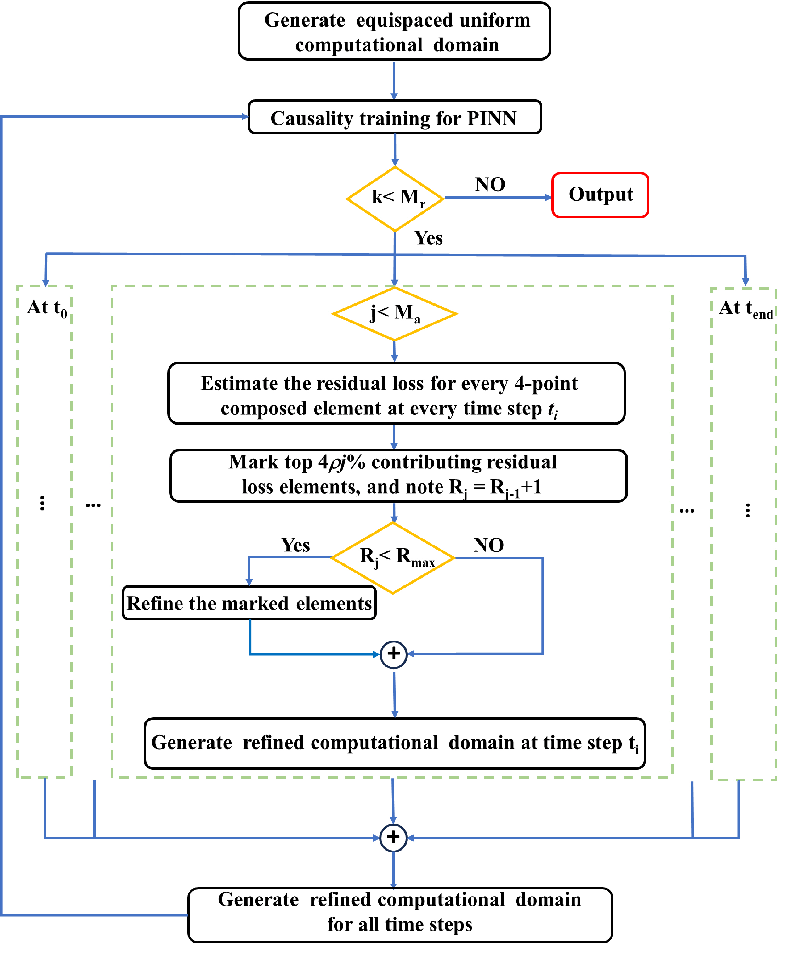
Figure 1: Flowchart of the proposed RBAR-causality approach.

We propose the following algorithm for implementing the Residual-Based Adaptive Refinement (RBAR) method in the context of causality:

Input: $\Omega$: Initial computational domain

$T=\{t_{1},\ldots,t_{N}\}$: Set of time steps

$M_{r}$: Maximum global refinement iterations

$M_{a}$: Maximum adaptive refinements per time step

$\rho$: Refinement threshold parameter

$\varepsilon$: Convergence tolerance

Output: $\mathcal{M}$: Optimized PINN model, $\Omega_{f}$: Final refined mesh

1

2Initialize PINN model $\mathcal{M}$ and set $\Omega_{0}=\Omega$;

3 $\mathcal{L}_{0}\leftarrow$ InitialTraining($\mathcal{M},\Omega_{0}$);

4

5for $k\leftarrow 1$ to $M_{r}$ do

6       $\Omega_{k}\leftarrow\Omega_{k-1}$;

7       for $t\in T$ do

8             for $j\leftarrow 1$ to $M_{a}$ do

9                   $\mathcal{L}_{r}\leftarrow$ ComputeResidualLoss($\mathcal{M},\Omega_{k},t$);

10                   $S_{j}\leftarrow$ IdentifyRefinementSet($\Omega_{k},\mathcal{L}_{r},\rho,j$);

11                   $\Omega_{k}\leftarrow$ ApplyHRefinement($\Omega_{k},S_{j}$);

12                  

13             end for

14            

15       end for

16      $\mathcal{M},\mathcal{L}_{k}\leftarrow$ CausalityTraining($\mathcal{M},\Omega_{k}$);

17      

18 end for

19

20$\Omega_{f}\leftarrow\Omega_{k}$;

21 return $\mathcal{M},\Omega_{f}$;

22

23

24 Function InitialTraining($\mathcal{M},\Omega$):

25       Perform initial causality training on $\mathcal{M}$ using $\Omega$;

26       return Initial loss $\mathcal{L}_{0}$;

27      

28

29

30Function ComputeResidualLoss($\mathcal{M},\Omega,t$):

31       Calculate residual loss for all points in $\Omega$ at time $t$;

32       return Residual loss $\mathcal{L}_{r}$;

33      

34

35

36Function IdentifyRefinementSet($\Omega,\mathcal{L}_{r},\rho,j,R_{max}$):

37       Select top $(4\rho j)\%$ of points with highest $\mathcal{L}_{r}$;

38       Retrieve the refinement level R for every point;

39       Note: R = R+1;

40       if $R<R_{max}$ then

41             refine the corresponding points;

42       end if

43      

44      return Refinement set $S_{j}$;

45      

46

47

48Function ApplyHRefinement($\Omega,S$):

49       Apply $h$-refinement to points in set $S$;

50       return Updated mesh $\Omega$;

51      

52

53

54Function CausalityTraining($\mathcal{M},\Omega$):

55       Perform causality training on $\mathcal{M}$ using refined mesh $\Omega$;

56       return Updated model $\mathcal{M}$, New loss $\mathcal{L}$;

57      

58

59

Algorithm 1 Enhanced RBAR-Causality Method

In each causality training cycle, we implement an adaptive learning rate scheduler based on the Stochastic Gradient Descent with Warm Restarts method proposed by Loshchilov and Hutter [26]. This approach dynamically adjusts the learning rate throughout the training process, following a cyclical pattern where the rate initially starts high, gradually decreases to a predefined value or zero, and then restarts. This cyclical strategy offers several advantages: it facilitates efficient exploration of the loss landscape in the early stages of each cycle, allows for fine-tuning and convergence to optimal value as the rate decreases, and helps the model escape suboptimal local minima through periodic restarts. By employing this technique, we significantly enhance the robustness of our RBAR-causality based PINNs framework, effectively mitigating the risk of convergence to erroneous solutions that may arise from consistently high learning rates, while also avoiding the premature convergence often associated with monotonically decreasing rates. Furthermore, this approach aligns well with the iterative nature of our RBAR-Causality method, as each refinement stage can benefit from a fresh cycle of the learning rate schedule, potentially leading to improved adaptation to the refined mesh structure.

3 Phase Field modeling employing Allen-Cahn equation

In this section, we derive a phase field model (PFM) based on the Allen-Cahn equation in both static and dynamic forms. We construct a two-phase PFM with a single order parameter $u$, beginning with the total Helmholtz free energy of the investigated systems:

$$\mathcal{F}=\int_{\Omega}fd\omega=\int_{\Omega}(Wg(u)+\frac{\kappa}{2}|\nabla u|^{2})d\omega.$$ (10)

Here, $W$ represents the energy barrier and $\kappa$ denotes the scale factor of the interfacial energy density. The function $g(u)=u^{2}(1-u)^{2}$ is the double well function, a fundamental component in phase field modeling [27, 28]. To describe the phase evolution, we employ the functional derivative of the Helmholtz free energy. Consequently, the corresponding Allen-Cahn equation for this system is given by:

$$\frac{\partial u}{\partial t}=-L_{\sigma}\frac{\delta\mathcal{F}}{\delta u}=-L_{\sigma}(2Wu(1-u)(1-2u)-\kappa\nabla^{2}u),$$ (11)

where $L_{\sigma}$ denotes the relaxation coefficient, which is proportional to the rate of phase evolution [29]. It is important to note that Eq. (11) describes a static co-existence of two phases with a finite-thickness interface [30]. To extend the model to dynamic systems with evolving phases, we introduce an additional driving force term to the static PFM:

$$\frac{\partial u}{\partial t} =-L_{\sigma}\left[2Wu(1-u)(1-2u)-\kappa\nabla^{2}u\right]+L_{\eta}\left[\frac{dP(u)}{du}f(u,\bm{x},t)\right]\$$ (12)

$$=-L_{\sigma}\left[2Wu(1-u)(1-2u)-\kappa\nabla^{2}u\right]+L_{\eta}\left[\frac{dP(u)}{du}c\right].$$

In this extended form, $L_{\eta}$ represents the scaling coefficient for the driving force term, and $f(u,\bm{x},t)$ is the driving force function depending on the order parameter $u$, spatial coordinates $\bm{x}$, and time $t$. For simplicity in this study, we assume $f(u,\bm{x},t)$ to be a constant $c$, representing a constant driving force. The term $\frac{dP(u)}{du}=u^{3}(10-15u+6u^{2})$ ensures that the driving force originates from the interface, as proposed by Wang et al. [31]. This formulation provides a comprehensive framework for modeling phase evolution in both static and dynamic contexts, capturing the interplay between interfacial energy, bulk free energy, and external driving forces.

4 Numerical results

In this section, we employ the proposed RBAR causality-based PINN in both static and dynamic cases with different initial morphology, i.e., plane interface and hump interface, respectively. The static and the dynamic cases are denoted with Eq. (11) and (12), respectively. The solutions obtained via our PINN framework are systematically benchmarked against finite element method (FEM) solution computed using COMSOL Multiphysics. Through comprehensive comparative analysis, we demonstrate the computational efficiency, numerical accuracy, and adaptive error correction capabilities of the RBAR causality-based PINN methodology.

The neural network architecture employed in this work comprises a feed forward fully connected network with a hyperbolic tangent activation function, including 5 hidden layers and 100 neurons in each hidden layer.

4.1 Quasi-static Allen-Cahn Equation

We conduct our numerical experiments in a three-dimensional spatio-temporal domain where $(t,x,y)\in[0,1]\times[0,1]\times[0,1]$. The initial discretization comprises 8000 uniformly distributed collocation points prior to refinement, as depicted in Figure 2(a). Our two-phase PFM simulation tracks the phase transition dynamics, with the full three-dimensional evolution shown in Figure 2(b). The static Allen-Cahn equation takes the form in Eq. (11). And we set the corresponding parameters: $L_{\sigma}=1$, $W=8\times 10^{-4}$, and $\kappa=1\times 10^{-4}$. The initial condition, illustrated in Figure 1(d), establishes a discrete plane interface at $x=0.5$ separating two phases: the red phase ($u=1$) and the blue phase ($u=0$). Following observations were made in the initial implementation of the framework which employs only RBAR (without causality training):

1. The mean loss using the Adam optimizer [32] converges to below $10^{-10}$ (see Figure 2(c)), yet significant discrepancies emerge between PINN predictions (see Figures 2(d-f)) and COMSOL FEM results (see Figures 2(g-i)).

2. While the interface evolves toward a finite width configuration (see Figure 2(g-i)), the current distribution of collocation points proves insufficient to accurately capture the interface width variations.

These limitations highlight the necessity for implementing the complete RBAR strategy to improve solution accuracy, particularly in regions with steep gradients near the phase interface.

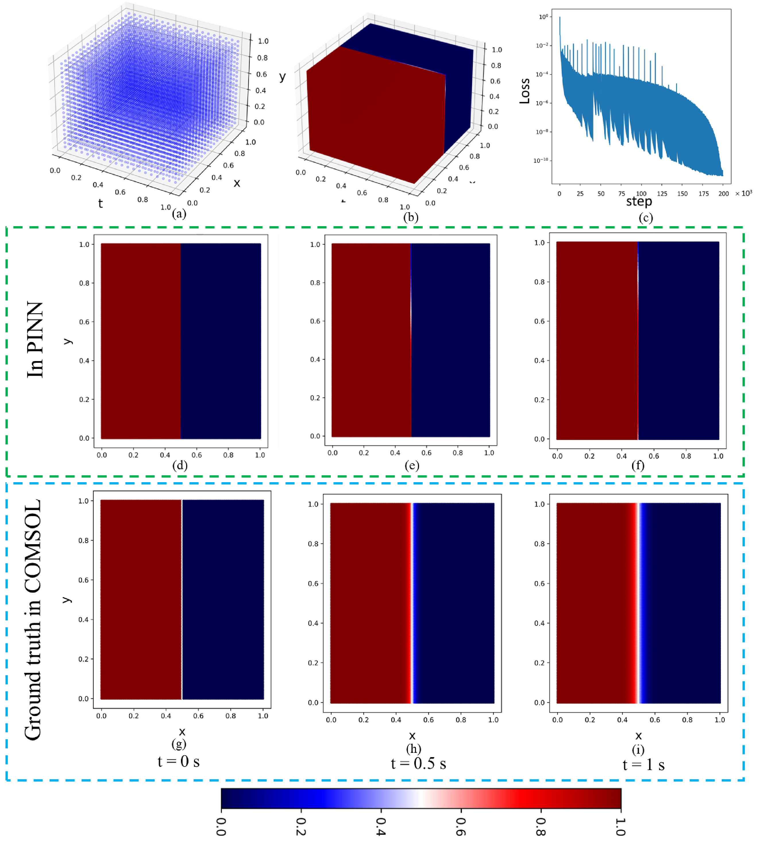
Figure 2: Static phase evolution results with planar interface configuration. (a) Initial computational domain discretized with 8,000 ($20\times 20\times 20$) uniformly distributed collocation points. (b) Three-dimensional phase morphology evolution simulated using the PINN framework. (c) History of the mean loss obtained using the Adam optimizer over 20,000 training iterations. (d-f) Phase morphology evolution predicted by PINN at t = 0 s, 0.5 s, and 1 s, respectively. (g-i) Corresponding phase morphology evolution computed using COMSOL FEM simulation at identical time points for direct comparison. Color scale represents phase parameter u, where red (u = 1) and blue (u = 0) indicate distinct phases.

Following a single iteration of the computational domain with the collocation points in Figure 2(a), an adaptive refinement was implemented employing the RBAR method, as shown in Figure 3(a). The refinement process automatically identified regions of highest residual loss, which predominantly occurred along the sharp phase interface. This adaptive point distribution proved crucial for several reasons:

1. Enhanced Resolution: The increased density of collocation points near the interface enabled accurate capture of the steep gradients characteristic of phase boundaries.

2. Improved Physics Representation: The refined mesh successfully resolved the interface widening phenomenon, as evidenced in Figure 3(d-f). The simulation results now demonstrate excellent agreement with the expected physical behavior.

3. Computational Efficiency: By concentrating computational resources in regions of high physical activity (i.e., the phase interface), RBAR optimizes the distribution of collocation points to maximize accuracy while minimizing computational overhead.

The effectiveness of RBAR lies in its ability to identify and adaptively refine regions where the PDE residuals are largest, thereby providing the PINN with the necessary spatial resolution to accurately characterize the underlying physics of the Allen-Cahn equation. This targeted refinement strategy proves particularly valuable for problems featuring localized phenomena such as moving interfaces and sharp gradients. The loss history with the RBAR PINNs framework is shown in Figure 3(c).

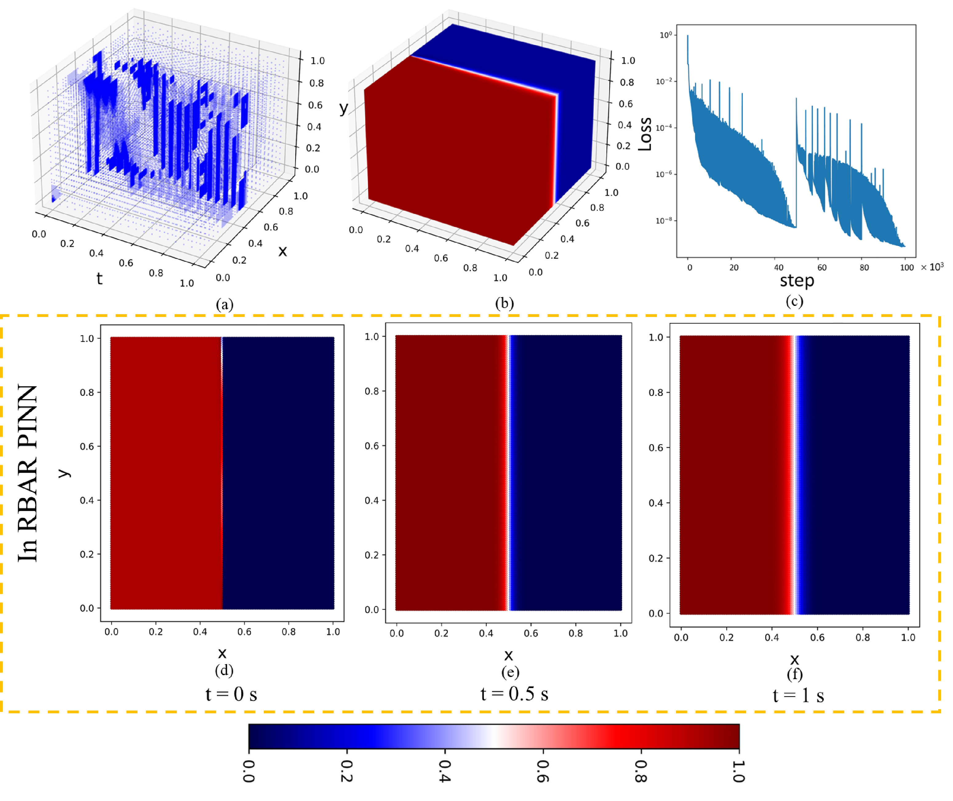
Figure 3: Static phase evolution results with planar interface using RBAR-enhanced PINN methodology. (a) Computational domain after RBAR refinement showing adaptive point distribution. (b) Three-dimensional visualization of phase morphology evolution computed using RBAR PINN. (c) Mean Adam loss evolution per collocation point over 100,000 total iterations, comprising 50,000 iterations pre-refinement and 50,000 post-RBAR implementation. (d-f) Phase morphology evolution captured by RBAR PINN at t = 0 s, 0.5 s, and 1 s, demonstrating interface dynamics.

4.2 Dynamic Allen-Cahn Equation

For the dynamic case analysis, we maintain the same computational domain configuration as established in the static case. The governing Allen-Cahn equation incorporates a constant driving force term as follows:

$$\frac{\partial u}{\partial t}=W\left[2u(1-u)(1-2u)\right]-\kappa\nabla^{2}u+L_{\eta}cu^{3}(10-15u+6u^{2}),$$ (13)

where $W=8\times 10^{-4}$, $\kappa=1\times 10^{-4}$, $L_{\eta}=0.01$, and $c=200$. The initial condition consists of a planar interface morphology. In this investigation of moving plane dynamics, we implement RBAR PINN without the causality training strategy. Impact of Refinement Strategies. Our observations are summarized as follows:

1. Without Refinement: As shown in Figure 4, the planar interface remains stationary, failing to capture the expected phase transition dynamics.

2. Uniform Refinement: Even after increasing the resolution from $20^{3}$ to $44^{3}$ collocation points (exceeding 8,100 total points), the interface exhibited no displacement despite 100,000 training iterations.

RBAR Implementation: Our optimal strategy consisted of an initial training phase with 50,000 iterations, followed by RBAR-guided domain refinement (illustrated in Fig. 4) which is the secondary training phase that has an additional 50,000 training iterations.

Only the RBAR-guided refinement successfully captured the phase transition dynamics. This outcome demonstrates that uniform refinement proves ineffective for solving the dynamic Allen-Cahn equation. The RBAR methodology not only enhances solution accuracy but also helps the PINN framework avoid convergence to incorrect solutions, highlighting its crucial role in capturing complex phase transition dynamics.

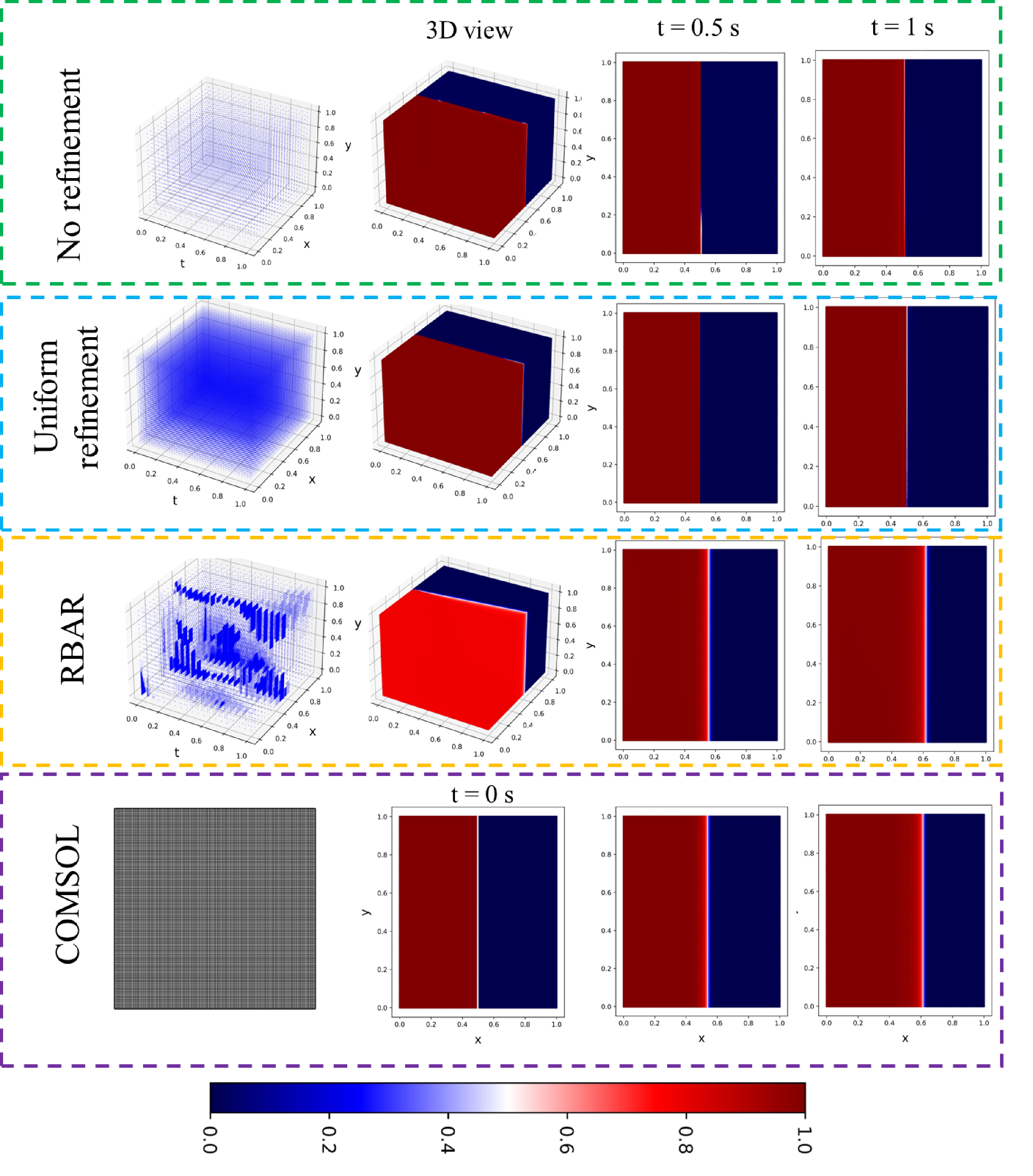
Figure 4: Comparative analysis of dynamic phase evolution with planar interface using different computational approaches: unrefined PINN simulation showing static interface behavior, uniform mesh refinement ($44^{3}$ collocation points) demonstrating persistent stagnation, RBAR-enhanced PINN capturing interface motion, and reference COMSOL FEM solution validating the dynamic evolution.

4.3 Simulating complex Morphology with Dynamic Equation

We next investigate the Allen-Cahn equation (Eq. 13) with a more challenging initial condition: a small hump (radius $r=0.02$) superimposed on the planar interface, as illustrated in Figure 5. The evolution of this small perturbation presents a significant computational challenge, even for RBAR-enhanced PINN implementations.

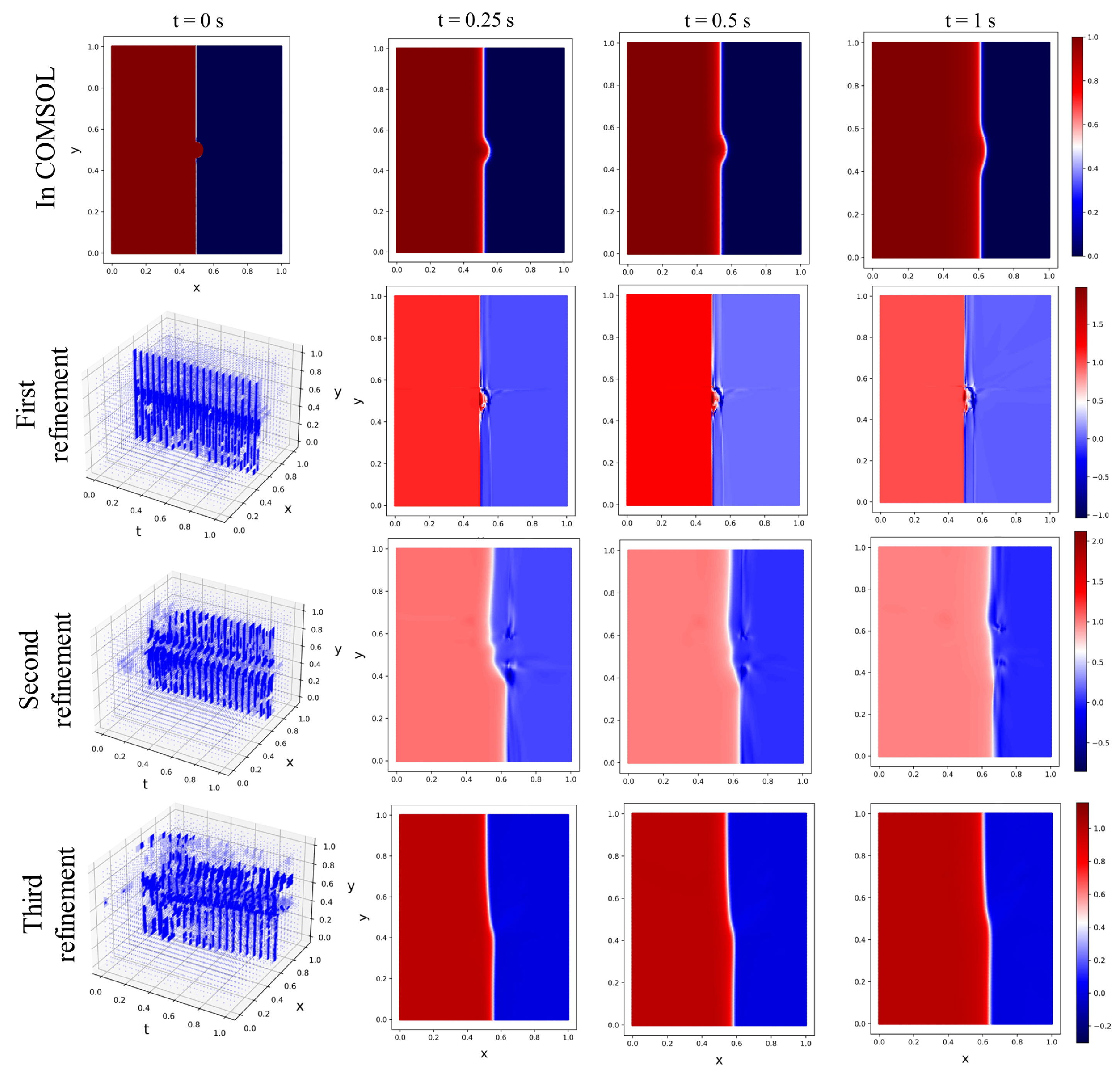
Figure 5: Comparative analysis of phase field evolution with initial hump morphology: COMSOL reference solution versus RBAR PINN results after first, second, and third refinement iterations, demonstrating progressive improvement in solution accuracy.

Limitations of RBAR-Only Implementation: Initial attempts using only RBAR refinement revealed significant challenges in accurately capturing the hump evolution. While multiple refinement iterations improved certain aspects of the solution—including better interface smoothness and phase-field values more strictly confined to the $[0,1]$ range—the predicted morphology deviated substantially from the COMSOL reference solution. Specifically, the characteristic hump structure disappeared as the interface evolved toward a planar configuration, indicating fundamental limitations of the RBAR-only approach for this dynamic case.

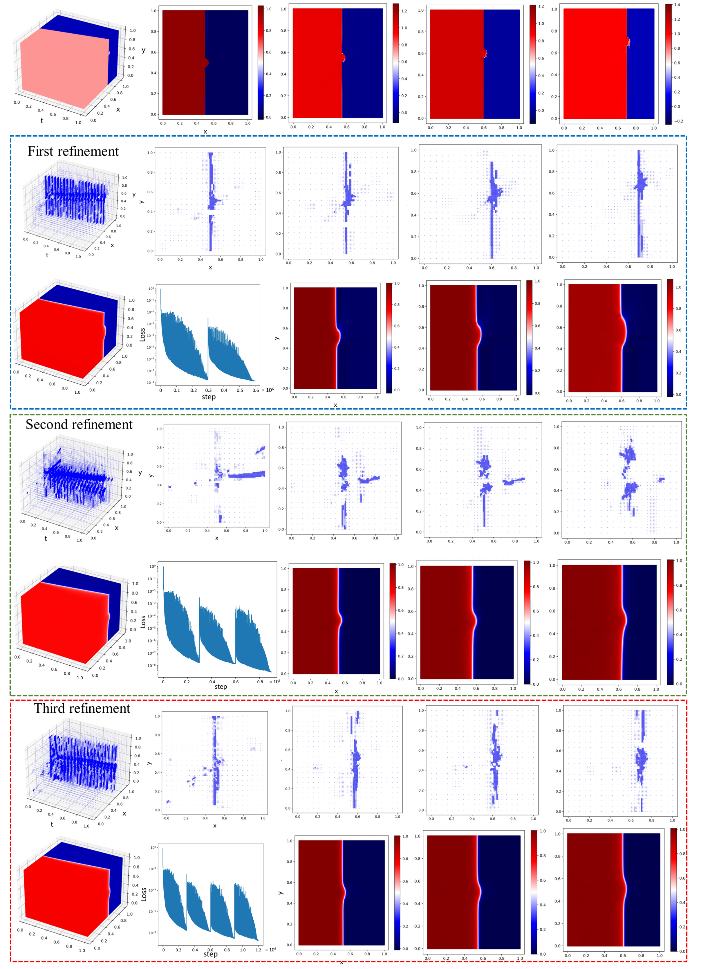
Figure 6: Evolution of phase-field solution using RBAR-causality combined PINN methodology: comparison of results with no refinement, first, second, and third refinement iterations, showing progressive improvement in accuracy.

To address these limitations, we developed a hybrid approach combining RBAR with causality training, as demonstrated in Figure 6. The implementation proceeded through two primary stages:

Initial Causality Training

The process began with 300,000 iterations using causality-based training. While the results demonstrated correct interface motion direction, they exhibited two significant limitations: (i) inadequate representation of hump growth dynamics, and (ii) substantial spatial overshoot, with interface positions appearing at $x\approx 0.6$ and $x\approx 0.7$ compared to the COMSOL reference positions at $x=0.5$ and $x=0.6$, respectively.

Iterative Refinement Process

Following the initial training, we implemented a systematic refinement procedure comprising: (i) initial refinement based on residual loss distribution, (ii) subsequent 300,000 iterations with causality training, revealing a notable “overshoot and relocate” phenomenon that demonstrates the method’s adaptive error correction capabilities, and (iii) two additional refinement cycles for solution fine-tuning. This iterative approach progressively improved solution accuracy while maintaining computational efficiency.

To elucidate the complementary roles of RBAR and causality training, we conducted detailed analysis of the early-time evolution (see Figure 7). The causality-training PINN accurately captures the initial morphology dynamics, matching COMSOL results in both interface position and hump structure. RBAR then identifies and refines regions of highest residual loss—primarily the interface and hump regions—providing enhanced spatial resolution where needed most. This synergistic interaction enables accurate capture of complex morphological features, elimination of spatial overshooting as well as correct positioning of the evolving interface

The combined methodology successfully reproduces the COMSOL reference solution, demonstrating the effectiveness of integrating RBAR refinement with causality training for challenging phase-field evolution problems.

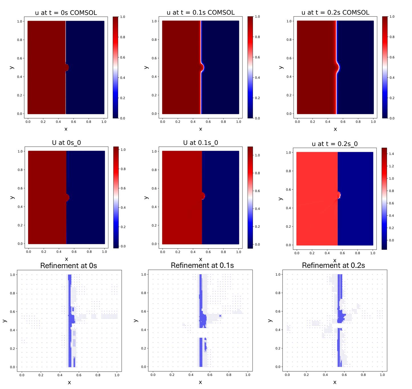
Figure 7: Comparative analysis of early-stage evolution (t = 0s, 0.1s, 0.2s) showing phase-field morphology obtained via COMSOL, causality training without refinement, and RBAR refinement patterns.

5 Conclusion

In this study, we introduce a novel methodology that combines RBAR (Residual-Based Adaptive Refinement) with causality-informed training in PINNs to solve spatio-temporal PDEs, with specific application to the phase field model (PFM) based on Allen-Cahn equations. Our analysis of the dynamic case with planar interfaces reveals that uniform refinement of the computational domain proves inefficient. Instead, the RBAR mechanism enables the PINN to overcome convergence to erroneous solutions by strategically allocating collocation points to capture interface evolution phenomena. However, we observed that RBAR alone proves insufficient for accurately resolving dynamic PFM cases with complex interfacial morphologies. The integration of causality-informed training with RBAR significantly enhances the framework’s capability to accurately reproduce temporal interface evolution, particularly in cases involving non-planar morphologies. During the iterative refinement and training process, we identify a characteristic overshoot and relocate phenomenon, which emerges from the synergistic interaction between RBAR and causality-informed training. This mechanism operates as follows: initially, RBAR concentrates collocation points in regions of high loss that have been partially resolved through causality training. Subsequently, the causality-informed training utilizes these strategically placed points to obtain accurate solutions at initial timesteps. These refined initial solutions then enable accurate prediction and tracking of interface evolution in subsequent timesteps.

While our current implementation focuses on dynamic Allen-Cahn equations, the proposed RBAR-causality framework is readily extensible to diverse spatio-temporal systems due to its generalized formulation. The RBAR methodology demonstrates simultaneous improvements in solution accuracy and computational efficiency. Furthermore, this combined RBAR causality-based PINN framework establishes a foundational methodology for future developments in PINN-based solutions of Phase Field Models.

Author contributions

Conceptualization: WW, SG, HHR
Investigation: WW, SG, HHR, TPW
Visualization: WW
Supervision: SG, HHR
Writing—original draft: WW
Writing—review & editing: WW, SG, HHR

Data and code availability

All codes and datasets will be made publicly available at https://github.com/Centrum-IntelliPhysics/PINNs-Causality-based-Adaptive-Refinement upon publication of the work.

Competing interests

The authors declare no competeting interest

References

- [1] M. Raissi, P. Perdikaris, G. E. Karniadakis, Physics-informed neural networks: A deep learning framework for solving forward and inverse problems involving nonlinear partial differential equations, Journal of Computational physics 378 (2019) 686–707.
- [2] E. Samaniego, C. Anitescu, S. Goswami, V. M. Nguyen-Thanh, H. Guo, K. Hamdia, X. Zhuang, T. Rabczuk, An energy approach to the solution of partial differential equations in computational mechanics via machine learning: Concepts, implementation and applications, Computer Methods in Applied Mechanics and Engineering 362 (2020) 112790.
- [3] A. D. Jagtap, E. Kharazmi, G. E. Karniadakis, Conservative physics-informed neural networks on discrete domains for conservation laws: Applications to forward and inverse problems, Computer Methods in Applied Mechanics and Engineering 365 (2020) 113028.
- [4] A. A. Ramabathiran, P. Ramachandran, SPINN: sparse, physics-based, and partially interpretable neural networks for PDEs, Journal of Computational Physics 445 (2021) 110600.
- [5] S. Goswami, C. Anitescu, S. Chakraborty, T. Rabczuk, Transfer learning enhanced physics informed neural network for phase-field modeling of fracture, Theoretical and Applied Fracture Mechanics 106 (2020) 102447.
- [6] A. D. Jagtap, G. E. Karniadakis, Extended physics-informed neural networks (XPINNs): A generalized space-time domain decomposition based deep learning framework for nonlinear partial differential equations, Communications in Computational Physics 28 (5) (2020).
- [7] J. Cho, S. Nam, H. Yang, S.-B. Yun, Y. Hong, E. Park, Separable PINN: Mitigating the curse of dimensionality in Physics-Informed neural networks, arXiv preprint arXiv:2211.08761 (2022).
- [8] S. Karumuri, R. Tripathy, I. Bilionis, J. Panchal, Simulator-free solution of high-dimensional stochastic elliptic partial differential equations using deep neural networks, Journal of Computational Physics 404 (2020) 109120.
- [9] B. Yu, et al., The deep Ritz method: a deep learning-based numerical algorithm for solving variational problems, Communications in Mathematics and Statistics 6 (1) (2018) 1–12.
- [10] E. Kharazmi, Z. Zhang, G. E. Karniadakis, Variational physics-informed neural networks for solving partial differential equations, arXiv preprint arXiv:1912.00873 (2019).
- [11] J. Sirignano, K. Spiliopoulos, DGM: A deep learning algorithm for solving partial differential equations, Journal of computational physics 375 (2018) 1339–1364.
- [12] Y. Yang, P. Perdikaris, Physics-informed deep generative models, arXiv preprint arXiv:1812.03511 (2018).
- [13] G. Pang, G. E. Karniadakis, Physics-informed learning machines for partial differential equations: Gaussian processes versus neural networks, Emerging Frontiers in Nonlinear Science (2020) 323–343.
- [14] L. P. Swiler, M. Gulian, A. L. Frankel, C. Safta, J. D. Jakeman, A survey of constrained Gaussian process regression: Approaches and implementation challenges, Journal of Machine Learning for Modeling and Computing 1 (2) (2020).
- [15] C. L. Wight, J. Zhao, Solving allen-cahn and cahn-hilliard equations using the adaptive physics informed neural networks, arXiv preprint arXiv:2007.04542 (2020).
- [16] A. Krishnapriyan, A. Gholami, S. Zhe, R. Kirby, M. W. Mahoney, Characterizing possible failure modes in physics-informed neural networks, Advances in Neural Information Processing Systems 34 (2021) 26548–26560.
- [17] R. Mattey, S. Ghosh, A novel sequential method to train physics informed neural networks for allen cahn and cahn hilliard equations, Computer Methods in Applied Mechanics and Engineering 390 (2022) 114474.
- [18] S. Wang, S. Sankaran, P. Perdikaris, Respecting causality is all you need for training physics-informed neural networks, arXiv preprint arXiv:2203.07404 (2022).
- [19] J. Yu, L. Lu, X. Meng, G. E. Karniadakis, Gradient-enhanced physics-informed neural networks for forward and inverse pde problems, Computer Methods in Applied Mechanics and Engineering 393 (2022) 114823.
- [20] C. Wu, M. Zhu, Q. Tan, Y. Kartha, L. Lu, A comprehensive study of non-adaptive and residual-based adaptive sampling for physics-informed neural networks, Computer Methods in Applied Mechanics and Engineering 403 (2023) 115671.
- [21] J. Jung, H. Kim, H. Shin, M. Choi, Ceens: Causality-enforced evolutional networks for solving time-dependent partial differential equations, Computer Methods in Applied Mechanics and Engineering 427 (2024) 117036.
- [22] S. Wang, Y. Teng, P. Perdikaris, Understanding and mitigating gradient flow pathologies in physics-informed neural networks, SIAM Journal on Scientific Computing 43 (5) (2021) A3055–A3081.
- [23] S. Wang, X. Yu, P. Perdikaris, When and why pinns fail to train: A neural tangent kernel perspective, Journal of Computational Physics 449 (2022) 110768.
- [24] L. McClenny, U. Braga-Neto, Self-adaptive physics-informed neural networks using a soft attention mechanism, arXiv preprint arXiv:2009.04544 (2020).
- [25] S. Goswami, C. Anitescu, T. Rabczuk, Adaptive fourth-order phase field analysis using deep energy minimization, Theoretical and Applied Fracture Mechanics 107 (2020) 102527.
- [26] I. Loshchilov, F. Hutter, Sgdr: Stochastic gradient descent with warm restarts, arXiv preprint arXiv:1608.03983 (2016).
- [27] C. Lin, H. Ruan, Phase-field modeling of scale roughening induced by outward growing oxide, Materialia 5 (2019) 100255.
- [28] N. Moelans, B. Blanpain, P. Wollants, An introduction to phase-field modeling of microstructure evolution, Calphad 32 (2) (2008) 268–294.
- [29] D. Fan, L.-Q. Chen, Computer simulation of grain growth using a continuum field model, Acta Materialia 45 (2) (1997) 611–622.
- [30] S. G. Kim, W. T. Kim, T. Suzuki, Phase-field model for binary alloys, Physical review e 60 (6) (1999) 7186.
- [31] S.-L. Wang, R. Sekerka, A. Wheeler, B. Murray, S. Coriell, R. Braun, G. McFadden, Thermodynamically-consistent phase-field models for solidification, Physica D: Nonlinear Phenomena 69 (1-2) (1993) 189–200.
- [32] D. P. Kingma, Adam: A method for stochastic optimization, arXiv preprint arXiv:1412.6980 (2014).