Spontaneous symmetry breaking induced by nonlinear interaction in a coupler supported by fractional diffraction

Abstract

In this paper we introduce a one-dimensional model of coupled fractional nonlinear Schrödinger equations with a double-well potential applied to one component. This study examines ground state (GS) solitons, observing spontaneous symmetry breaking (SSB) in both the actuated field and the partner component due to linear coupling. Numerical simulations reveal symmetric and asymmetric profiles arising from a slightly asymmetric initial condition. Asymmetry is influenced by nonlinearities, potential depth, and coupling strength, with self-focusing systems favoring greater asymmetry. Fractional diffraction affects the amplitude and localization of symmetric profiles and the stability of asymmetric ones. We identify critical Lévy index values for generating coupled GS solitons. Stability analysis of unstable, centrally asymmetric GS solitons demonstrates oscillatory dynamics, providing new insights into SSB in fractional systems and half-trapped solitons.

I Introduction

Solitons, which are localized wave packets, retain their shape and stability during propagation as a result of a precise equilibrium between dispersion and nonlinearity. This phenomenon occurs in a wide range of physical systems, including optical fibers, plasmas, and Bose-Einstein condensates (BECs), where nonlinear interactions effectively counteract the dispersive forces. The formation and stability of solitons have been extensively explored in nonlinear systems, providing a rich framework for understanding wave dynamics under nontrivial conditions [1]. Due to their ability to preserve their structure and interact with other solitons without losing coherence, solitons have become a central topic in the study of complex wave phenomena [2]. Moreover, the analysis of solitons is essential for advancing the understanding of more intricate nonlinear behaviors, especially when additional influences, such as fractional diffraction, are introduced.

Fractional diffraction, which extends classical diffraction by introducing fractional-order derivatives in the governing equations, brings about novel dynamics that influence soliton behavior. The application of the fractional Laplacian operator induces long-range interactions and anomalous diffusion, significantly complicating the solitons’ stability, localization, and interaction properties [3, 4]. These nonlocal effects can reshape soliton propagation, often creating conditions that promote the onset of more intricate phenomena, such as spontaneous symmetry breaking (SSB). The study of fractional diffraction and its impact on soliton dynamics has gained considerable attention, providing deeper insights into wave propagation in complex and nonlocal media [5, 6, 7, 8, 9, 10, 11, 12, 13, 14, 15, 16, 17, 18].

Indeed, SSB plays a crucial role in physics, describing how a system initially in a symmetric configuration evolves into an asymmetric state due to internal dynamics or external perturbations [19]. In the context of coupled nonlinear systems, SSB can give rise to asymmetric soliton states, even when the governing equations retain symmetry. The interplay between SSB and fractional diffraction is especially compelling, as the nonlocal effects induced by fractional diffraction can shift the power balance between coupled components, leading to symmetry disruption and the formation of localized structures [20, 21].

Another interesting effect is the half-trapped solitons, which emerge in systems governed by coupled nonlinear Schrödinger equations (NLSE), where a confining potential is applied to only one of the fields, while the second (partner) field remains unconfined [22]. In such configurations, localization occurs in the unconfined field solely due to the coupling between the two fields, as the second field would otherwise remain delocalized in the absence of this interaction. The coupling induces a mutual localization effect, allowing the partner field to inherit the confinement properties of the first, resulting in a spatially localized soliton state that would not be achievable without the coupled dynamics. In this sense, Ref. [23] has presented the study on Anderson localization induced by interaction in linearly coupled binary BECs. Also, the phenomenon of SSB induced by interaction in linearly coupled binary BECs has been previously reported in Ref. [24]. The objective of the present work is to investigate how linear coupling induces spontaneous symmetry breaking (SSB) in a system characterized by fractional diffraction. Specifically, this study aims to explore the interplay between linear coupling and fractional diffraction effects, examining how these interactions influence the emergence and characteristics of SSB in such a nonlinear system.

The structure of the paper is as follows: The subsequent section introduces the theoretical model. Section III is dedicated to the numerical simulations and the analysis of their results. Finally, Section IV presents our conclusions.

II Theoretical model

We begin the analysis by considering the propagation of light in a system composed of coupled planar waveguides, described by the rescaled model of the coupled nonlinear fractional Schrödinger equation (f-NLSE) [25, 26, 27, 28]

$$i\dfrac{\partial}{\partial z}\phi_{1} =\frac{1}{2}\left[-\dfrac{\partial^{2}}{\partial x^{2}}\right]^{\alpha/2}\phi_{1}+\left(g_{1}|\phi_{1}|^{2}+g_{12}|\phi_{2}|^{2}\right)\phi_{1}$$

$$\quad+U(x)\phi_{1},$$

$$i\dfrac{\partial}{\partial z}\phi_{2} =\frac{1}{2}\left[-\dfrac{\partial^{2}}{\partial x^{2}}\right]^{\alpha/2}\phi_{2}+\left(g_{2}|\phi_{2}|^{2}+g_{12}|\phi_{1}|^{2}\right)\phi_{2},$$ (1)

where $z$ represents the normalized propagation distance, $x$ denotes the transverse coordinate, and $\alpha$ is the Lévy index (LI). The functions $\phi_{1,2}(x,z)$ describe the field amplitudes corresponding to components (waveguides) 1 and 2, respectively. The parameters $g_{1,2}$ represent the Kerr self-interaction coefficients, while $g_{12}$ denotes the nonlinear interaction coefficient between the components. The sign of the nonlinearity parameters, $g_{1,2}<0$ or $g_{1,2}>0$, characterizes the system as exhibiting either self-focusing or self-defocusing nonlinearity, respectively. Model (1) describes a conservative optical system. In this context, the dynamically invariant quantity of total power (or norm) is expressed as

$$P\equiv P_{1}+P_{2}=\int_{-\infty}^{+\infty}\left(|\phi_{1}|^{2}+|\phi_{2}|^{2}\right)dx,$$ (2)

where $P_{1}$ and $P_{2}$ are the individual powers of each component.

The LI $\alpha$, which ranges from $0<\alpha\leq 2$, is featured in the fractional diffraction operator $(-\partial{{}^{2}}/\partial x{{}^{2}})^{\alpha/2}$, representing the kinetic energy term in the Schrödinger equation. When $\alpha=2$, this operator reduces to the standard 1D Laplacian, resulting in the coupled NLSE with quadratic diffraction in Eq. (1). By using the direct and inverse Fourier transform, the fractional Laplacian in Eq. (1) can be rewritten in terms of the integral operator [29, 30]

$$\left(-\dfrac{\partial^{2}}{\partial x^{2}}\right)^{\alpha/2}\phi(x,z) =\frac{1}{2\pi}\iint dkdx^{\prime}|k|^{\alpha}$$

$$\times \exp\left[ik(x-x^{\prime})\right]\phi(x^{\prime},z).$$ (3)

In the self-focusing f-NLSE, which can be derived from the equation of motion for the component $\phi_{2}$ with $g_{2}<0$ and $g_{1,2}=0$ (see Eq. (1)), collapse occurs when $\alpha\leq 1$, inhibiting the formation of stable localized solutions [31].

In this work we consider an external potential acting only on component 1, which has the function of spatially confining the respective optical field. Systems with two components, where only one of them is trapped, have been previously studied in linearly coupled NLSE. In these cases, the so-called half-trapped systems exhibit ground state and dipole modes under harmonic oscillator-type confinement [32], and Anderson localization when a quasi-periodic optical lattice is considered [23]. In this context, to induce symmetry breaking, we employ a double-well potential, defined by

$$U(x)=-U_{0}\left[\cosh(x+x_{0})^{-2}+\cosh(x-x_{0})^{-2}\right],$$ (4)

where $U_{0}$ denotes the potential depth, and $x_{0}$ specifies the position of the local minimum for each of the wells. For simplicity, in our simulations we will assume $x_{0}=3$. Similar potentials have been utilized to generate asymmetric states in the study of ultracold gases, where a nonpolynomial Schrödinger equation (NPSE), derived from a variational approach, is employed to model the longitudinal dynamics of a BEC confined in the transverse direction [33]. Also, in Ref. [24], the induction of SSB in a half-trapped system described by a linearly coupled NLSE was achieved through a double-well potential (similar to Eq. (4)) in framework of binary BECs. Unlike previous works, this study proposes investigating the induction of SSB in fractional half-trapped optical systems with nonlinear interaction, which is generally present in high-intensity optical field configurations.

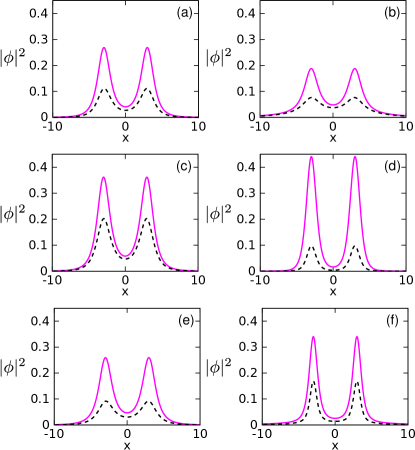
Figure 1: Symmetric profiles of the coupled states. The components $|\phi_{1}(x)|^{2}$ and $|\phi_{2}(x)|^{2}$ which were obtained numerically by Eq. (1) are arranged in magenta solid lines and black dotted lines. The parameters used in (a) are: $P=2$, $U_{0}=1$, $g_{1}=g_{2}=3$, $g_{12}=-3$ and $\alpha=1.5$. The other panels are obtained with the same parameters as in (a), but for (b) $g_{1}=g_{2}=5$, (c) $P=3$, (d) $U_{0}=2$, (e) $g_{12}=-2.5$, and (f) $\alpha=0.5$.

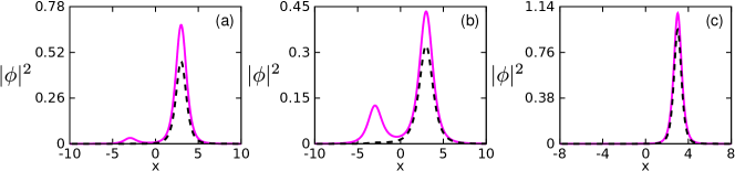
Figure 2: Asymmetric profiles of the coupled states $|\phi_{1}(x)|^{2}$ and $|\phi_{2}(x)|^{2}$ versus $x$, obtained in the same configurations as in Fig. 1(a), but for $g_{1}=g_{2}=2$ (a), $g_{2}=2$ (b), and $g_{12}=-5$ (c).

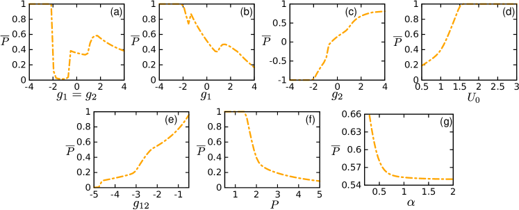
Figure 3: Comparison between the individual powers $P_{1}$ and $P_{2}$, considering the relative power $\overline{P}=\left(P_{1}-P_{2}\right)/P$ versus the parameters (a) $g_{1}=g_{2}$, (b) $g_{1}$, (c) $g_{2}$, (d) $U_{0}$, (e) $g_{12}$, (f) $P$ and (g) $\alpha$. The parameters used here are: (a) $P=2$, $U_{0}=1$, $\alpha=1.5$ and $g_{12}=-2$; (b) the same as in (a) but for $g_{2}=1$; (c) the same as in (a) but for $g_{1}=1$; (d) $P=2$, $g_{1}=g_{2}=2$, $\alpha=1.5$, and $g_{12}=-2$; (e) the same as in (d) but for $U_{0}=1$; (f) the same as in (d) but for $U_{0}=1$; and (g) the same as in (d).

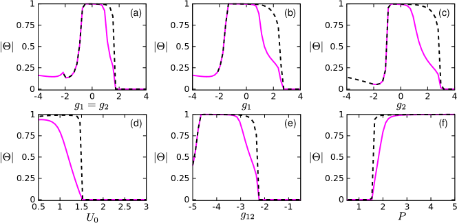
Figure 4: Absolute values of the asymmetry rate $|\Theta|$ versus (a) $g_{1}=g_{2}$, (b) $g_{1}$, (c) $g_{2}$, (d) $U_{0}$, (e) $g_{12}$, and (f) $P$, considering the same settings as the respective panels in Fig. 3. The results of the components $\phi_{1}$ and $\phi_{2}$, corresponding to $|\Theta_{1}|$ and $|\Theta_{2}|$ are shown in solid magenta lines and dotted black lines, respectively.

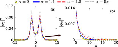
Figure 5: Effect of fractional diffraction ($\alpha$) on the symmetric coupled state of component 2 ($\phi_{2}$). The profiles were obtained numerically through Eq. (1) with $g_{1}=g_{2}=2$, $g_{12}=-2$, $U_{0}=1$ and $P=2$.

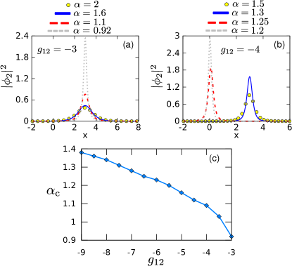
Figure 6: The same as Fig. 5, but for asymmetric coupled state of component 2 ($\phi_{2}$) with (a) $g_{12}=-3$ and (b) $g_{12}=-4$. The asymmetric profiles have $\Theta_{2}(\alpha=1.5)=1$, $\Theta_{2}(\alpha=1.3)=1$, $\Theta_{2}(\alpha=1.25)=0.33$ and $\Theta_{2}(\alpha=1.2)=0.13$. (c) Critical values of LI ($\alpha_{c}$) versus $g_{12}$, considering $g_{1}=g_{2}=2$, $U_{0}=1$ and $P=2$. Only singular states are obtained with $\alpha<\alpha_{c}$.

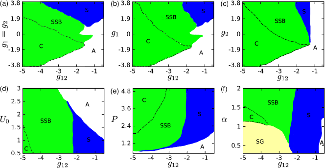
Figure 7: Phase diagram of coupled states. The symmetric phase (S) is represented by the blue filled area while spontaneous symmetry breaking (SSB) is represented by the green filled area. The empty areas (A) represent the regions where coupled states are not allowed ($P_{1}=0$ or $P_{2}=0$). Unstable delta-type configurations (SG) are represented by the yellow filled area, while the region enclosed by the black dashed line indicates the central asymmetric configurations (C). The other parameters used here are: (a) $P=2$, $U_{0}=1$ and $\alpha=1.5$; (b) $P=2$, $U_{0}=1$, $g_{2}=1$ and $\alpha=1.5$; (c) $P=2$, $U_{0}=1$, $g_{1}=1$ and $\alpha=1.5$; (d) $P=2$, $g_{1}=g_{2}=2$ and $\alpha=1.5$; (e) $U_{0}=1$, $g_{1}=g_{2}=2$ and $\alpha=1.5$; and (f) $P=2$, $U_{0}=1$ and $g_{1}=g_{2}=2$.

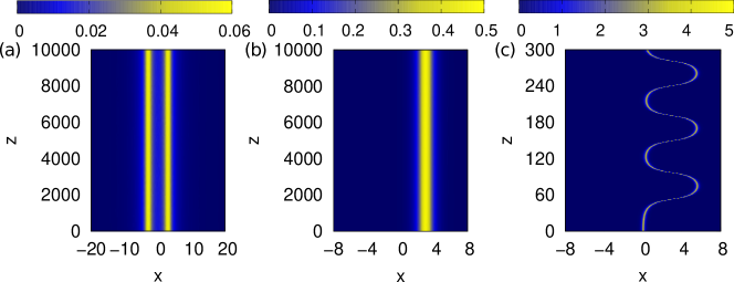
Figure 8: Evolution of stable GS solitons (a) symmetric and (b) asymmetric. (c) Typical unstable evolution of a central asymmetric profile. In all panels, only the results for the field density $|\phi_{2}|^{2}$ are presented. All results presented refer to component 2. The other parameters used here are: $U_{0}=1$, $P=2$, $g_{1}=g_{2}=1$ (a) $\alpha=0.9$ and $g_{12}=-1.5$; (b) $\alpha=1.5$ and $g_{12}=-3$; and (c) $\alpha=1.3$ and $g_{12}=-4.5$.

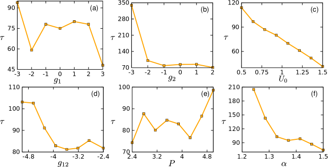
Figure 9: Oscillation periods of the unstable central asymmetric solitons corresponding to component 2. The parameters used are: (a) $P=2$, $U_{0}=1$, $\alpha=1.5$, $g_{2}=1$ and $g_{12}=-4.5$; (b) the same as in (a) but for $g_{2}=1$; (c) $P=2$, $U_{0}=1$, $\alpha=1.5$, $g_{1}=g_{2}=2$ and $g_{12}=-5$; (d) $P=2$, $U_{0}=1$, $\alpha=1.5$, and $g_{1}=g_{2}=-1.5$; (e) $U_{0}=1$, $\alpha=1.5$, $g_{1}=g_{2}=2$ and $g_{12}=-4.5$; and (f) $P=2$, $U_{0}=1$, $g_{12}=-5$, and $g_{1}=g_{2}=-1.5$.

III Numerical simulations

Deriving analytical solutions for coupled f-NLSEs is particularly challenging due to the interplay of nonlinearity, coupling, and fractional diffraction. Recent studies indicate that the inclusion of the fractional Laplacian operator $(-\partial{{}^{2}}/\partial x{{}^{2}})^{\alpha/2}$ significantly complicates the process of obtaining general analytical solutions [34, 35, 36, 37, 38, 25, 39, 40], making numerical methods the preferred approach in such scenarios. Consequently, in this work, solutions are determined numerically by integrating the equations of motion (1) using both imaginary-time and real-time propagation methods.

The imaginary-time propagation method promotes the ground states (GS) by replacing the coordinate $z\rightarrow-iz$ in Eqs. (1). In this sense, the propagation in imaginary “time” (respective of the propagation coordinate $z$) acts as a relaxation process over an input profile $\phi_{1,2}^{\textrm{In}}(x,z=0)$, whose result converges to the lowest energy state related to the configuration of Eq. (1). To find the GS solitons, we start the simulations with the slightly asymmetric Gaussian input profile

$$\phi_{1,2}^{\textrm{In}}(x,z=0)=\mathcal{P}\exp\left[-\frac{(x-\sigma)^{2}}{2}\right],$$ (5)

where $\mathcal{P}$ is the normalization constant defined according to the total power (2) and $\sigma=0.01$ is the asymmetry parameter. During the relaxation process, both individual powers are free, obeying only the normalization condition (2). Therefore, the GS solitons exhibit $P_{1,2}=[0,\,P]$, with $P_{1}+P_{2}=P$. The real-time propagation method is employed to investigate the dynamics of the GS solitons, which are used as input profiles, from which their behavior along $z$ is studied. Both numerical methods are performed by a second-order split-step algorithm used to separately integrate the linear and nonlinear terms of the system of Eq. (1). The diffractive part $\sim(-\partial{{}^{2}}/\partial x{{}^{2}})^{\alpha/2}$ is integrated using Eq. (3), while the nonlinear part presents an analytical solution. The integration of both terms is performed simultaneously in each iteration step [41].

For self-focusing systems ($g_{1,2}<0$), even in the absence of coupling ($g_{12}=0$), model (1) presents GS solitons for both components. However, when self-defocusing systems are considered ($g_{1,2}>0$), only component 1 presents GS solutions in the absence of coupling. Therefore, in this configuration, the localization of component 2 occurs only when it is induced by the partner field coupling. Additionally, the simulations show that the coupling determines the appearance of localized solutions. For example, considering $g_{12}<0$, the coupling acts as a confining mechanism, similar to a spatially inhomogeneous nonlinearity [39, 26, 42]. Conversely, when $g_{12}>0$, the coupling operates as a delocalizing factor, inhibiting the formation of localized solutions such as GS solitons.

In the numerical simulations, we found coupled GS solitons that present spatial symmetry with respect to the $x$-axis. These symmetric GS solitons present two identical peaks centered at $\pm x_{0}$. In Fig. 1, we studied the influence of nonlinearities ($g_{1},g_{2}$), total power ($P$), potential depth ($U_{0}$), coupling intensity ($g_{12}$) and LI ($\alpha$) on the coupled symmetrical profiles obtained in the self-defocusing regime. Specifically, the Fig. 1(a) shows a typical example of symmetrical GS solitons. We observe that increasing the nonlinearities ($g_{1}=g_{2}$) leads to a broadening of the profiles and a reduction in amplitude, as shown in Fig. 1(b). The increase in total power also promotes a rise in the amplitude of both components (see Fig. 1(c)). In Fig. 1(d), we present the profiles resulting from the increase in the depth of the double-well potential. Note that component 1 has a much higher amplitude than component 2, with peaks that are almost completely separated from each other. A slight reduction in the coupling intensity ($|g_{12}|$) also promotes the amplitude difference between the components, as shown in Fig. 1(e). Fig. 1(f) was produced with $\alpha=0.5$, which, compared to Fig. 1(a), shows that the reduction in symmetric fractional diffraction causes a narrowing of the peaks in the GS solitons.

Our numerical analysis reveals the presence of spatially asymmetric GS solutions, characterized either by peaks of differing amplitudes or by a single peak displaced from the center of the double-well potential. Therefore, for certain parameters (detailed below), SSB occurs, resulting in GS solitons characterized by $|\phi_{1,2}(x,z)|^{2}\neq|\phi_{1,2}(-x,z)|^{2}$. In Fig. 2, we present three examples of asymmetric GS solitons obtained from the variation of $g_{1}=g_{2}$, $g_{2}$, and $g_{12}$, considering the configuration shown in Fig. 1. It is observed that reducing the nonlinearities of both components in self-defocusing systems can induce SSB. In particular, reducing the nonlinearity of component 2 is sufficient by itself to promote SSB. Furthermore, the coupling also influences the symmetry type of the coupled GS solitons, where an increase in $|g_{12}|$ promotes asymmetry. It is important to highlight that both profiles were obtained in self-defocusing systems, where the absence of coupling renders the formation of coupled GS solitons impossible. As a result, the SSB (and localization) observed in component 2 are induced by component 1.

The asymmetric profiles in Fig. 2 are generated with $\sigma=0.01$, and therefore, their highest peaks (or single peak) are shifted in the direction of $x>0$. Numerical simulations show that the same asymmetric GS solitons are obtained using $\tilde{\sigma}=-\sigma$, but with the inversion of the direction of the highest peaks, i.e., $|\phi_{1,2}^{\sigma}(x,z)|^{2}=|\phi_{1,2}^{\tilde{\sigma}}(-x,z)|^{2}$. Therefore, the set of these asymmetric GS solitons obtained with different symmetry parameters ($\sigma$, $\tilde{\sigma}$) forms degenerate states of Eq. (1).

Based on Figs. 1 and 2, it is evident that the individual powers of components 1 and 2 can vary depending on the selected parameters. This behavior is effectively captured by the relative power $\overline{P}=\left(P_{1}-P_{2}\right)/P$, where $\overline{P}>0$ ($\overline{P}<0$) indicates that $P_{1}>P_{2}$ ($P_{2}>P_{1}$), while $\overline{P}=0$ represents equality between the individual powers. In Fig. 3(a), we present the influence of both nonlinearities ($g_{1}=g_{2}$) on $\overline{P}$. We observe that in the strong self-focusing regime, $g_{1}=g_{2}<-2$, only component 1 presents a localized solution. This behavior is abruptly modified for $g_{1}=g_{2}>-2$, where both components present similar values. In the entire analyzed region, we find $P_{1}\geq P_{2}$. To analyze the effects of $g_{1}$ on the individual powers of the GS solitons, we fix the nonlinearity of component 2 ($g_{2}=1$). Similar to the previous case (see Fig. 3(a)), it is observed that in the strong self-focusing regime the power of component 1 is favored. However, increasing $g_{1}$ leads $P_{1}\rightarrow P_{2}$, as shown in Fig. 3(b). The same analysis performed for $g_{2}$ produces very different results. In the configuration where the nonlinearity of component 1 is fixed at $g_{1}=1$, shown in Fig. 3(c), the decrease of $g_{2}$ favors $P_{2}$. For example, considering $g_{2}<-2$, only component 2 presents a localized solution.

Fig. 3(d) shows the effects of the double-well potential depth on the individual powers. We observe that increasing $U_{0}$ causes an imbalance between the individual powers. In this configuration, all GS solitons obtained with $U_{0}>1.6$ exhibit only component 1 ($P_{1}=P$, $P_{2}=0$). Similarly, reducing the coupling strength between the components leads to the vanishing of component 2, as observed in Fig. 3(e). From Fig. 3(f), we observe that increasing the total power $P$ results in GS solitons with similar individual powers. Conversely, under the same conditions, only component 1 is obtained when $P<1.4$. Unlike the previous analyses, the influence of fractional diffraction on the individual powers is relatively small. In general, increasing $\alpha$ induces slight changes in the individual powers, reducing the imbalance between the components.

Fig. 3 shows how the individual norms are affected by the parameter variations, without making any reference to SSB. To investigate this behavior, it is important to quantify the intensity of the spatial SSB presented by the GS solitons. Here, we use the asymmetry ratio, defined as

$$\Theta_{1,2}=\frac{\int_{0}^{+\infty}|\phi_{1,2}|^{2}dx-\int_{-\infty}^{0}|\phi_{1,2}|^{2}dx}{P_{1,2}},$$ (6)

where $\Theta$ has values from $-1$ to $1$. Asymmetric GS solitons are characterized by $|\Theta|>0$, while symmetric profiles have $|\Theta|=0$. In particular, values of $|\Theta|$ close to limit $1$ indicate that the GS soliton is confined by a single potential well (4), as shown in Fig. 2(c).

In Fig. 4, we present the same analysis as in Fig. 3, but considering the influence of the parameters on the (a)symmetry region. We observe that the SSB is present for both components when $-2.1<g_{1}=g_{2}<1.8$. Similarly, when $g_{2}$ is fixed, the system exhibits SSB for $g_{1}<2.5$. With $g_{1}$ fixed, the SSB region for both components expands slightly with variations in $g_{2}$. In general, we observe that the decrease in nonlinearities favors the emergence of SSB. These results are presented in Figs. 4(a-c). The depth of the double wells, $U_{0}$, also plays an important role in the symmetry of the GS solitons. Fig. 4(d) shows the behavior of $|\Theta|$ versus $U_{0}$, where we observe that only asymmetric profiles are found for $U_{0}<1.52$. Under the same conditions, Fig. 4(e) demonstrates that strong coupling also promotes SSB, restricting symmetric profiles to weak couplings ($|g_{1,2}|<-2.1$). Finally, Fig. 4(f) illustrates the influence of total power on the symmetry of the GS solitons, clearly showing that an increase in $P$ leads to asymmetric profiles. Our findings indicate that modifying the LI parameter exclusively is insufficient to affect the symmetry of the coupled GS solitons. Despite this, fractional diffraction influence the GS solitons in complex ways and, therefore, is not discussed in this analysis. We detail these behaviors below.

We begin by presenting the influence of fractional diffraction on the symmetric GS solitons. As shown in Fig. 1(f), a reduction in LI leads to GS solitons with higher amplitudes, as detailed in Fig. 5(a). In addition, the tails of the symmetric GS solitons undergo significant changes, as a reduction in LI causes them to extend over longer distances (see Fig. 5(b)).

In Fig. 6, we detail the effects of fractional diffraction on the asymmetric GS solitons. In this configuration, the decrease in LI also leads to an increase in the amplitude of the GS solitons. Unlike the symmetric case, when SSB is present, the decrease in LI introduces a critical value $\alpha_{c}$, for which no GS profile is obtained with $\alpha<\alpha_{c}$. For instance, in the configuration shown in Fig. 6(a) with coupling $g_{12}=-3$, all profiles obtained with $\alpha<0.92$ are unstable delta-type solutions with either $P_{1}$ or $P_{2}=0$. Therefore, there are certain limiting values for LI ($\alpha_{c}$), for which model (1) does not support GS solitons. Increasing the coupling intensity in such systems can lead to the emergence of asymmetric GS solitons localized near the center of the double-well potential, as shown in Fig. 6(b). These central asymmetric profiles exhibit a relatively small asymmetry ratio compared to other asymmetric profiles. For example, considering $g_{12}=-4$, the standard asymmetric profiles for component 2 exhibit $|\Theta_{2}|\approx 1$, while the central asymmetric profiles obtained with $\alpha=1.2$ and $1.25$ show $|\Theta_{2}|=0.13$ and $0.33$, respectively. Numerical simulations demonstrate that increasing the coupling intensity also raises the critical values $\alpha_{c}$. This behavior is investigated in Fig. 6(c), where the nonlinear pattern of the critical LI, $\alpha_{c}(g_{12})$, is observed.

Considering the influence of coupling associated with other parameters on the symmetry of the GS solitons, we extend the investigation by means of existence diagrams, where the regions of existence of symmetric, asymmetric, and central asymmetric GS solitons are determined. Furthermore, we investigate the region where the formation of GS solitons in both components does not occur. The existence diagrams of $g_{1}=g_{2}$, $g_{1}$, $g_{2}$, $U_{0}$, $P$ and $\alpha$ versus $g_{12}$ are displayed in Fig. 7. The regions of existence for the different GS solitons are depicted in Fig. 7(a), based on the variations in nonlinearities and the coupling between the components. We observe that the symmetric profiles are favored in strongly decocting systems in a weak coupling regime. On the other hand, the SSB appears in the strong coupling regime. In general, the optical system tends not to support the GS solitons in the self-focusing regime with weak coupling. By fixing $g_{1}$ or $g_{2}$, similar results are found for the asymmetry regions. However, in this configuration, the symmetry region is drastically reduced. Notably, when $g_{1}$ is fixed, weak coupling prevents the formation of GS solitons, even under a strong self-interaction regime in component 2. These findings are presented in Figs. 7(b-c).

The diagram in the plane $(g_{12},U_{0})$, shown in Fig. 7(d), demonstrates that SSB is favored by strong coupling in systems with deep potentials. For $U_{0}<2.5$, symmetric profiles are also observed. In this configuration, central asymmetric profiles are limited to strongly coupled systems associated with a shallow external potential. The absence of GS solitons is observed in regimes of strong coupling associated with a deep potential. In Fig. 7(e), we present the results from the diagram ($g_{12}$, $P$). As observed previously, increasing the coupling strength favors SSB. In this configuration, GS solitons are not supported in systems with low total power in a weakly coupled regime. The diagram corresponding to the variation of the LI ($g_{12}$, $\alpha$) produces different results (see Fig. 7(f)). In this configuration, we observe that delta-type profiles are favored in systems with small LI in a strong self-coupling regime. Note that these states are not present in the previous diagrams, showing their connection with the fractional diffraction and the coupling intensity between the components. SSB is observed in systems with large LI values in a strong coupling regime. In the weak coupling regime, symmetric profiles are found. In particular, a small region where SG profiles are not found is observed for weakly coupled systems obtained with small LI.

In the previous analyses, we presented the regions of existence for symmetric, asymmetric, central asymmetric, and delta-type profiles. An important question to investigate is the dynamic stability of these different profiles. For real-time propagation, we considered the coupled GS solitons as input profiles, but randomly perturbed them by $3\%$ of their amplitudes. In these configurations, dynamic stability against small perturbations is confirmed when both components propagate without exhibiting abrupt changes in their shapes or amplitudes over a distance of $z=10000$. As previously shown, the delta-type profiles are unstable and exhibit only one component with non-zero individual power. Extensive numerical simulations demonstrate the stability of all symmetric and asymmetric (standard) profiles investigated. Despite the random noise introduced into the amplitudes, both profiles evolve without significant modifications to their shapes. In Fig. 8(a-b), we present examples of the stable evolution of GS solitons for component 2. In both cases, component 1 shows similar results, which are not detailed here.

In contrast, the central symmetric GS solitons present unstable evolution. The dynamics of these profiles present coherent oscillations around the minimum of one of the potential wells ($\pm x_{0}$). In the case of the central asymmetric profiles that initially present $\Theta_{1,2}>0$, the oscillatory dynamics occurs in the direction of $x>0$. Similarly, for those that present $\Theta_{1,2}<0$, the oscillations occur in the opposite direction, as shown in Fig. 8(c). We also investigated the oscillatory dynamics of the central symmetric profiles by considering the period of the initial oscillations ($\tau$) with variations in the parameters $g_{1}$, $g_{2}$, $U_{0}$, $g_{12}$, $P$ and $\alpha$. Figs. 9(a-b) show the effects of $g_{1}$ and $g_{2}$ on the oscillation period of the GS profiles corresponding to component 2. Generally, an increase in nonlinearities leads to a reduction in the oscillation period. When considering the depth of the double-well potential, we observe that the oscillation period decreases as the potential depth increases, as illustrated in Fig. 9(c). When the coupling is varied (see Fig. 9(d)), the oscillation period is seen to increase under strong coupling conditions. Fig. 9(e) demonstrates that the oscillations of the optical system are sensitive to an increase in the total power. This behavior arises due to the relationship between the total power and the system’s energy. Finally, in Fig. 9(f), we investigated the influence of fractional diffraction on the oscillation period, observing that an increase in LI leads to shorter oscillation periods.

IV Conclusion

We introduce a one-dimensional model of coupled f-NLSE with a double-well potential applied to only one of the components. In this configuration, we investigate GS solitons, where SSB was observed in both the actuated field and the partner component, highlighting asymmetry induction via coupling. Numerical simulations reveal the existence of both symmetric and asymmetric profiles, initiated from a slightly asymmetric initial condition. The individual powers and the intensity of the SSB are significantly influenced by the nonlinearities, potential depth, and nonlinear coupling. Generally, asymmetry is favored in self-focusing (or weakly self-defocusing) systems with strong coupling. Variations in fractional diffraction affect the amplitude and tails of the coupled symmetric GS solitons, while in asymmetric profiles, fractional diffraction influences the localization position and dynamic stability. Additionally, we identified critical values that define the minimum LI necessary to produce coupled GS solitons. Diagrams were employed to illustrate the regions where different types of GS solitons exist and where the model fails to support localized solutions. The stability of the GS solitons was assessed through direct simulations. For unstable cases, characterized solely by centrally asymmetric GS solitons, the oscillatory dynamics were analyzed, showing the impact of various parameters on the oscillation period of these profiles. This work aims to contribute new insights into SSB in fractional systems, particularly by elucidating the sparsely explored topic of half-trapped fractional systems.

References

- Agrawal [2013] G. Agrawal, ed., Nonlinear Fiber Optics (Fifth Edition), Optics and Photonics (Academic Press, Boston, 2013) p. vii.
- Kivshar and Agrawal [2003] Y. S. Kivshar and G. P. Agrawal, Optical Solitons, edited by Y. S. Kivshar, G. P. Agrawal, and G. P. Agrawal (Academic Press, Burlington, 2003) pp. xv–xvi.
- Longhi [2015] S. Longhi, Opt. Lett. 40, 1117 (2015).
- Malomed [2021a] B. A. Malomed, Photonics 8, 10.3390/photonics8090353 (2021a).
- Yao and Liu [2018] X. Yao and X. Liu, Photon. Res. 6, 875 (2018).
- Dong and Huang [2018] L. Dong and C. Huang, Opt. Express 26, 10509 (2018).
- Zhu et al. [2020] X. Zhu, F. Yang, S. Cao, J. Xie, and Y. He, Opt. Express 28, 1631 (2020).
- Li et al. [2021] P. Li, B. A. Malomed, and D. Mihalache, Opt. Lett. 46, 3267 (2021).
- Che et al. [2021] W. Che, F. Yang, S. Cao, Z. Wu, X. Zhu, and Y. He, Phys. Lett. A 413, 127606 (2021).
- Wu et al. [2022] Z. Wu, K. Yang, Y. Zhang, X. Ren, F. Wen, Y. Gu, and L. Guo, Chaos Soliton Fract. 158, 112010 (2022).
- Bo et al. [2023] W.-B. Bo, R.-R. Wang, Y. Fang, Y.-Y. Wang, and C.-Q. Dai, Nonlinear Dyn. 111, 1577 (2023).
- Zhong and Yan [2023] M. Zhong and Z. Yan, Commun. Phys. 6, 92 (2023).
- Wang et al. [2023] J. Wang, Q. Wu, C. Du, L. Yang, P. Xue, and L. Fan, Phys. Lett. A 471, 128794 (2023).
- Chen et al. [2024] S. Chen, Y. He, X. Peng, X. Zhu, and Y. Qiu, Physica D 457, 133966 (2024).
- Wang et al. [2024] L. Wang, J. Zeng, and Y. Zhu, Physica D 465, 134144 (2024).
- Yu et al. [2024] F. Yu, L. Li, J. Zhang, and J. Yan, Physica D 460, 134089 (2024).
- Bai et al. [2024] X. Bai, R. Yang, J. Chen, J. Bai, and H. Jia, Phys. Scr. 99, 035224 (2024).
- Zhai et al. [2024] Y. Zhai, R. Li, and P. Li, Acta Opt. Sin. 44, 0519002 (2024).
- Kevrekidis et al. [2008] P. G. Kevrekidis, D. J. Frantzeskakis, and R. Carretero-González, eds., in Emergent Nonlinear Phenomena in Bose-Einstein Condensates (Springer Berlin, Heidelberg, 2008).
- Zeng et al. [2023] L. Zeng, M. R. Belić, D. Mihalache, J. Li, D. Xiang, X. Zeng, and X. Zhu, Physica D 456, 133924 (2023).
- He et al. [2024] X. He, Y. Zhai, Q. Cai, R. Li, and P. Li, Chaos Solitons Fract. 186, 115258 (2024).
- Hacker and Malomed [2021a] N. Hacker and B. A. Malomed, Symmetry 13, 10.3390/sym13030372 (2021a).
- dos Santos and Cardoso [2021] M. C. P. dos Santos and W. B. Cardoso, Phys. Rev. E 103, 052210 (2021).
- dos Santos and Cardoso [2023] M. C. P. dos Santos and W. B. Cardoso, Nonlinear Dyn. 111, 3653 (2023).
- Zeng and Zeng [2020] L. Zeng and J. Zeng, Chaos, Solitons & Fractals 140, 110271 (2020).
- Li et al. [2022] S. Li, Y. Bao, Y. Liu, and T. Xu, Chaos, Solitons & Fractals 162, 112484 (2022).
- Ur-Rehman and Ahmad [2022] S. Ur-Rehman and J. Ahmad, Opt. Quantum Electron. 54, 640 (2022).
- Ahmad et al. [2023] J. Ahmad, S. Rani, N. B. Turki, and N. A. Shah, Results in Physics 52, 106761 (2023).
- Laskin [2000a] N. Laskin, Phys. Rev. E 62, 3135 (2000a).
- Laskin [2000b] N. Laskin, Phys. Lett. A 268, 298 (2000b).
- Malomed [2021b] B. A. Malomed, Photonics 8, 353 (2021b).
- Hacker and Malomed [2021b] N. Hacker and B. A. Malomed, Symmetry-Basel 13, 372 (2021b).
- Miranda et al. [2022] B. M. Miranda, M. C. dos Santos, and W. B. Cardoso, Phys. Lett. A 452, 128453 (2022).
- Zhang et al. [2015] Y. Zhang, X. Liu, M. R. Belić, W. Zhong, Y. Zhang, and M. Xiao, Phys. Rev. Lett. 115, 180403 (2015).
- Zhang et al. [2016] Y. Zhang, H. Zhong, M. R. Belić, Y. Zhu, W. Zhong, Y. Zhang, D. N. Christodoulides, and M. Xiao, Laser Photon. Rev. 10, 526 (2016).
- Zhong et al. [2016] W.-P. Zhong, M. R. Belić, B. A. Malomed, Y. Zhang, and T. Huang, Phys. Rev. E 94, 012216 (2016).
- Chen et al. [2018] M. Chen, S. Zeng, D. Lu, W. Hu, and Q. Guo, Phys. Rev. E 98, 022211 (2018).
- Chen et al. [2019] M. Chen, Q. Guo, D. Lu, and W. Hu, Commun. Nonlinear Sci. Numer. Simul. 71, 73 (2019).
- Zeng et al. [2021] L. Zeng, M. R. Belić, D. Mihalache, Q. Wang, J. Chen, J. Shi, Y. Cai, X. Lu, and J. Li, Chaos, Solitons & Fractals 152, 111406 (2021).
- dos Santos [2024] M. C. dos Santos, Chaos, Solitons & Fractals 183, 114916 (2024).
- Yang [2010] J. Yang, Nonlinear Waves in Integrable and Nonintegrable Systems (Society for Industrial and Applied Mathematics, 2010).
- dos Santos et al. [2024] M. C. dos Santos, B. A. Malomed, and W. B. Cardoso, Chin. J. Phys. 89, 1474 (2024).