Robust Bayes-assisted Confidence Regions

Abstract

The Frequentist, Assisted by Bayes (FAB) framework aims to construct confidence regions that leverage information about parameter values in the form of a prior distribution. FAB confidence regions (FAB-CRs) have smaller volume for values of the parameter that are likely under the prior, while maintaining exact frequentist coverage. This work introduces several methodological and theoretical contributions to the FAB framework. For Gaussian likelihoods, we show that the posterior mean of the parameter of interest is always contained in the FAB-CR. As such, the posterior mean constitutes a natural notion of FAB estimator to be reported alongside the FAB-CR. More generally, we show that for a likelihood in the natural exponential family, a transformation of the posterior mean of the natural parameter is always contained in the FAB-CR. For Gaussian likelihoods, we show that power law tails conditions on the marginal likelihood induce robust FAB-CRs, that are uniformly bounded and revert to the standard frequentist confidence intervals for extreme observations. We translate this result into practice by proposing a class of shrinkage priors for the FAB framework that satisfy this condition without sacrificing analytical tractability. The resulting FAB estimators are equal to prominent Bayesian shrinkage estimators, including the horseshoe estimator, thereby establishing insightful connections between robust FAB-CRs and Bayesian shrinkage methods.

Keywords: confidence intervals, exact coverage, prior information, uniformly bounded intervals, shrinkage, horseshoe.

1 Introduction

Let $Y\in\mathcal{Y}$ be a random variable with a probability density function $f_{\theta}$ where $\theta\in\Theta\subseteq\mathbb{R}^{d}$ is a parameter of interest. For a given $\alpha\in(0,1)$, we are interested in providing a confidence region $C_{\alpha}(Y)\subseteq\Theta$ for $\theta$, with exact coverage probability

$$\Pr(\theta\in C_{\alpha}(Y)\mid\theta)=1-\alpha$$ (1)

for any $\theta\in\Theta$. Let $\mathrm{vol}(C_{\alpha}(Y))=\int_{\theta^{\prime}\in C_{\alpha}(Y)}d\theta^{\prime}$ denote the volume of the confidence region. For a given parameter $\theta$, using the Ghosh-Pratt identity (Pratt, 1961; Ghosh, 1961), the expected volume of the confidence region is given by

$$\mathbb{E}[\mathrm{vol}(C_{\alpha}(Y))|\theta] =\int_{\mathcal{Y}}\mathrm{vol}(C_{\alpha}(y))f_{\theta}(y)dy=\int_{\Theta}\Pr(\theta^{\prime}\in C_{\alpha}(y)|\theta)d\theta^{\prime},$$ (2)

where $\Pr(\theta^{\prime}\in C_{\alpha}(y)|\theta)$ is the probability of false coverage for $\theta^{\prime}\neq\theta$. One may have some information about plausible values for the unknown parameter $\theta$. When that is the case, it may be desirable to allow for larger volumes for values of $\theta$ that are thought to be less likely, in exchange for smaller volumes for values of $\theta$ that are thought to be more likely. Following Pratt (1961, 1963), we operationalise this through a distribution $\pi$ on $\theta$, for which we aim to find the confidence region procedure $C_{\alpha}$ that minimises the (Bayes) expected volume

$$R(C_{\alpha})=\iint_{\mathcal{Y}\times\Theta}\mathrm{vol}(C_{\alpha}(y))f_{\theta}(y)dy\pi(d\theta)$$ (3)

under the (frequentist) constraint (1). Such approach, coined “Frequentist, Assisted by Bayes” (FAB) by Yu and Hoff (2018) has been used in a number of articles (Brown et al., 1995; Puza and O’Neill, 2006; Farchione and Kabaila, 2008; Kabaila and Giri, 2013; Hoff and Yu, 2019; Kabaila and Farchione, 2022; Hoff, 2023; Kabaila, 2024) in order to obtain smaller valid confidence regions, called FAB confidence regions (FAB-CR), for parameters of interest.

Owing to Eq. 2, when $\pi$ is a proper probability distribution, the Neyman-Pearson lemma implies that the confidence region $C_{\alpha}(y)$ takes the form

$$C_{\alpha}(y)=\{\theta\mid y\in A_{\alpha}(\theta)\}$$ (4)

where the acceptance region $A_{\alpha}(\theta)$ is given by a sublevel set of the log-likelihood ratio

$$A_{\alpha}(\theta)=\left\{y\mid\log\left(\frac{f(y)}{f_{\theta}(y)}\right)\leq k_{\alpha}(\theta)\right\}$$ (5)

where $f(y)=\int_{\Theta}f_{\theta}(y)\pi(d\theta)$ is the marginal density of $Y$ under the prior $\pi$ and $k_{\alpha}(\theta)$ is such that $\Pr(Y\in A_{\alpha}(\theta)\mid\theta)=\Pr(\theta\in C_{\alpha}(Y)\mid\theta)=1-\alpha$. For any $\theta_{0}$, $A_{\alpha}(\theta_{0})$ is the acceptance region, at significance level $\alpha$, of the Neyman-Pearson test of the null hypothesis $H_{0}:\theta=\theta_{0}$ against the alternative $H_{1}:\theta\sim\pi$, when $Y\mid\theta\sim f_{\theta}$.

An illustration of such approach when $Y\mid\theta\sim\mathcal{N}(\theta,0.1)$ is given in Fig. 1.

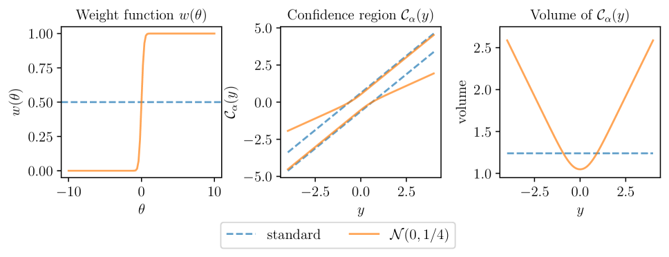
Figure 1: Comparison of the standard and FAB procedures under the prior $\mathcal{N}(0,1/4)$ when $Y\mid\theta\sim\mathcal{N}(\theta,0.1)$. The Gaussian prior results in confidence regions that are shorter than the standard one when $y$ is close to zero, but that grow unbounded as $|y|$ increases.

The standard confidence interval (CI) for the mean of a Gaussian with known variance is compared to the FAB-CR under a prior $\theta\sim\mathcal{N}(0,1/4)$. The standard CI has constant length, while the FAB-CR has smaller length when $y\simeq 0$. Whatever the choice of the prior, FAB-CRs have the correct frequentist coverage. A limitation of using the FAB approach is that the volume of the associated confidence region may not be uniformly bounded. This is the case with the Gaussian prior, as $\mathrm{vol}(C_{\alpha}(y))\to\infty$ as $|y|\to\infty$. Some modifications of the FAB approach have been proposed to alleviate this (Farchione and Kabaila, 2008; Hoff and Yu, 2019), but a general framework for providing uniformly bounded confidence regions is missing.

Another object of interest, which has not been investigated in the FAB literature, is the focal point of the collection of nested FAB-CRs $(C_{\alpha}(y))_{\alpha\in(0,1)}$, defined (assuming $\lim_{\alpha\to 1}\mathrm{vol}(C_{\alpha}(y))=0$) as

$$\widehat{\theta}^{\mathrm{FAB}}(y)=\bigcap_{\alpha\in(0,1)}C_{\alpha}(y).$$ (6)

The random variable $\widehat{\theta}^{\mathrm{FAB}}(Y)$, which always lies within the FAB-CR $C_{\alpha}(Y)$, may naturally be used as an estimator for the parameter of interest $\theta$, and reported together with the FAB-CR.

The contributions of this paper are as follows:

• We show that for Gaussian likelihoods, under mild assumptions on the prior $\pi$, the focal point $\widehat{\theta}^{\mathrm{FAB}}(y)$ of the FAB-CRs $(C_{\alpha}(y))$ is the posterior mean $\mathbb{E}[\theta\mid Y=y]$;

• The above result is extended to likelihoods in the natural exponential family; a closed-form expression for $\widehat{\theta}^{\mathrm{FAB}}(y)$ is given, in terms of the cumulant function and posterior mean of the natural parameter of the NEF;

• In the Gaussian likelihood case, we show that, if the marginal density $f(y)$ has power-law tails, the FAB-CRs are uniformly bounded and revert to the usual confidence interval as $|y|$ goes to infinity

• In the Gaussian likelihood case, we further propose a class of shrinkage priors that lead to CRs that (i) have an analytical expression for $f(y)$, allowing for a simple evaluation of the FAB-CRs, (ii) are uniformly bounded and (iii) are shrunk towards zero, encouraging sparsity. The resulting focal point is a shrinkage estimator that admits as special case many Bayesian estimators proposed in the literature, in particular the one based on the horseshoe prior (Carvalho et al., 2010), providing useful connections between shrinkage priors and robust FAB-CRs.

This article is organised as follows. In Section 2, we consider the Gaussian likelihood case, identifying both the focal point of the FAB-CRs, and sufficient conditions for robust FAB-CRs. In Section 3, we describe a class of prior that leads to a tractable, robust FAB-CR procedure, and draw connections with the Bayesian shrinkage literature. In Section 4, we consider more generally likelihoods in the natural exponential family, giving an expression for the focal point in this case.

2 Gaussian likelihood with known variance

Consider here a Gaussian likelihood,

$$f_{\theta}(y)=\frac{1}{\sqrt{2\pi\sigma^{2}}}\exp\left(-\frac{(y-\theta)^{2}}{2\sigma^{2}}\right)$$

where $y\in\mathbb{R}$, $\theta\in\mathbb{R}$ and $\sigma>0$ is assumed known here.

Assumption 2.1.

Assume $\pi(d\theta)$ is a non-degenerate Borel measure on $\mathbb{R}$, such that $\pi(A)<\infty$ for any Borel set $A$ of $\mathbb{R}$, and $0<\int_{\mathbb{R}}f_{\theta}(y)\pi(d\theta)<\infty$ for any $y\in\mathbb{R}$. We will refer to $\pi$ as the prior distribution.

Remark 2.1.

In most cases discussed in this paper, $\pi$ will be a probability distribution on $\mathbb{R}$, with $\int_{\mathbb{R}}\pi(d\theta)=1$. But 2.1 also allows for the use of improper priors with $\int\pi(d\theta)=\infty$, such as $\pi(d\theta)=d\theta$. The finiteness of $f(y)=\int_{\mathbb{R}}f_{\theta}(y)\pi(d\theta)$ guarantees that the posterior distribution $\pi(d\theta\mid y)=\frac{f_{\theta}(y)\pi(d\theta)}{f(y)}$ is proper. Note however that $f(y)$ is not a proper density function if $\pi(d\theta)$ is not a probability distribution. We will use a slight abuse of language, and call $f(y)$ the marginal likelihood, even when $\pi$ is not a probability distribution. The fact that $\pi(d\theta)$ need not be a (proper) probability distribution was already mentioned by Pratt (1963). The degenerate case $\pi(d\theta)=\delta_{\theta_{1}}$ for some $\theta_{1}\in\mathbb{R}$ is excluded from 2.1; this case has been covered in details by Pratt (1961, 1963).

Denote $\ell_{\theta}(y)=\log f_{\theta}(y)$ the log-likelihood and $\ell(y)=\log f(y)$ the log-marginal likelihood under some prior distribution $\pi$ satisfying 2.1. Let $\lambda_{\theta}(y)=\ell(y)-\ell_{\theta}(y)$ the log-likelihood ratio, and recall that the confidence region $C_{\alpha}(y)$ is obtained by inversion of the acceptance region $A_{\alpha}(\theta)=\left\{y\mid\lambda_{\theta}(y)\leq k_{\alpha}(\theta)\right\}$. Let

$$\widehat{\theta}(y)=\mathbb{E}[\theta|y]=y+\sigma^{2}\ell^{\prime}(y)$$ (7)

be the posterior mean of $\theta$ given $y$ under the prior $\pi$. We have the following result, that states that the acceptance regions $A_{\alpha}(\theta)$ are intervals, whose bounds are continuous and differentiable functions, and the FAB-CR $C_{\alpha}(y)$ contains the posterior mean under the prior $\pi$.

Theorem 2.1.

Assume $\pi(d\theta)$ satisfies 2.1. Then, for any $\theta_{0}\in\mathbb{R}$, the function $\lambda_{\theta_{0}}(y)=\ell(y)-\ell_{\theta_{0}}(y)$ is a strictly convex function of $y$ with

$$\arg\min_{y\in\mathbb{R}}\lambda_{\theta_{0}}(y)=\widehat{\theta}^{-1}(\theta_{0}).$$

Let $\alpha\in(0,1)$. The acceptance region $A_{\alpha}(\theta_{0})$ is an interval $[\underline{A}_{\alpha}(\theta_{0}),\overline{A}_{\alpha}(\theta_{0})]$, where $\underline{A}_{\alpha}(\theta_{0})<\widehat{\theta}^{-1}(\theta_{0})<\overline{A}_{\alpha}(\theta_{0})$. Let

$$w_{\alpha}(\theta)=\frac{1}{\alpha}\Phi\left(\frac{\underline{A}_{\alpha}(\theta)-\theta}{\sigma}\right)\in[0,1].$$ (8)

The functions $\underline{A}_{\alpha}(\theta)$, $\overline{A}_{\alpha}(\theta)$ and $w_{\alpha}(\theta)$ are all continuously differentiable on $\mathbb{R}$.

Let $y\in\mathbb{R}$. The confidence regions $C_{\alpha}(y)$ are given by

$$C_{\alpha}(y)=\{\theta\mid\underline{A}_{\alpha}(\theta)=\theta-\sigma z_{1-\alpha w_{\alpha}(\theta)}\leq y\leq\theta+\sigma z_{1-\alpha(1-w_{\alpha}(\theta))}=\overline{A}_{\alpha}(\theta)\},$$ (9)

and the focal point (6) of the FAB-CRs, assuming $\lim_{\alpha\to 1}\mathrm{vol}(C_{\alpha}(y))=0$, is given by

$$\widehat{\theta}^{\mathrm{FAB}}(y)=\widehat{\theta}(y)=\mathbb{E}[\theta\mid y].$$

Proof.

For any $\theta_{0}\in\mathbb{R}$, the function

$$\lambda_{\theta_{0}}(y)=\lambda_{0}(y)-\frac{y\theta_{0}}{\sigma^{2}}+\frac{{\theta_{0}}^{2}}{2\sigma^{2}}$$

is differentiable, with derivative

$$\lambda^{\prime}_{\theta_{0}}(y)=\lambda^{\prime}_{0}(y)-\frac{\theta_{0}}{\sigma^{2}}.$$

From Tweedie’s formula, one has

$$\lambda^{\prime}_{0}(y) =\ell^{\prime}(y)+\frac{y}{\sigma^{2}}=\frac{1}{\sigma^{2}}\mathbb{E}[\theta\mid y],$$

$$\lambda^{\prime\prime}_{0}(y) =\ell^{\prime\prime}(y)+\frac{1}{\sigma^{2}}=\frac{1}{\sigma^{4}}\mathrm{var}(\theta\mid y).$$

As the prior $\pi$ is non-degenerate, $\mathrm{var}(\theta\mid y)>0$, hence $\lambda_{0}$ (and $\lambda_{\theta_{0}}$, for any $\theta_{0}$) are strictly convex and $\lambda^{\prime}_{0}(y)$ and $\widehat{\theta}(y)$ are strictly increasing and bijective functions. Solving $\lambda^{\prime}_{\theta_{0}}(y_{0})=0$ yields $y_{0}={\widehat{\theta}}^{-1}(\theta_{0})\in A_{\alpha}(\theta_{0})$, and therefore $\widehat{\theta}(y)\in C_{\alpha}(y)$ for all $\alpha\in(0,1)$. The strict convexity of $\lambda_{\theta_{0}}$ also implies that $A_{\alpha}(\theta_{0})$ is an interval, written $[\underline{A}_{\alpha}(\theta_{0}),\overline{A}_{\alpha}(\theta_{0})]$, where the functions $\underline{A}_{\alpha}(\theta)$ and $\overline{A}_{\alpha}(\theta)$ satisfy the identities

$$\lambda_{\theta}(\overline{A}_{\alpha}(\theta)) =\lambda_{\theta}(\underline{A}_{\alpha}(\theta))$$ (10)

$$\Phi\left(\frac{\overline{A}_{\alpha}(\theta)-\theta}{\sigma}\right)-\Phi\left(\frac{\underline{A}_{\alpha}(\theta)-\theta}{\sigma}\right) =1-\alpha.$$ (11)

Writing $w_{\alpha}(\theta)$ as in Eq. 8 together with Eq. 4 gives Eq. 9. Finally, Eq. 11 implies that $\underline{A}_{\alpha}(\theta)=h_{\theta}(\overline{A}_{\alpha}(\theta))$ where

$$h_{\theta}(u)=\theta+\sigma\Phi^{-1}\left(\Phi\left(\frac{u-\theta}{\sigma}\right)-(1-\alpha)\right).$$ (12)

$\underline{A}_{\alpha}(\theta)$ and $w_{\alpha}(\theta)$ can be expressed as the composition of $\overline{A}_{\alpha}(\theta)$ by a continuous and differentiable function. Hence it is enough to prove the continuity and differentiability of $\overline{A}_{\alpha}(\theta)$. $\overline{A}_{\alpha}(\theta)$ is the solution to the implicit equation

$$G(\theta,\overline{A}_{\alpha}(\theta))=0,$$

where

$$G(\theta,u)=\lambda_{\theta}(u)-\lambda_{\theta}\left(h_{\theta}(u)\right).$$

Note that $h_{\theta}(u)$ is differentiable, with $h^{\prime}_{\theta}(u)>0$. We have

$$\frac{\partial G(\theta,u)}{du} =\lambda^{\prime}_{\theta}(u)-\lambda^{\prime}_{\theta}\left(h_{\theta}(u)\right)\times h^{\prime}_{\theta}(u).$$

Additionally, $\lambda^{\prime}_{\theta}(\overline{A}_{\alpha}(\theta))>0$ and $\lambda^{\prime}_{\theta}(\underline{A}_{\alpha}(\theta))<0$. Hence

$$\left.\frac{\partial G(\theta,u)}{du}\right|_{(\theta,\overline{A}_{\alpha}(\theta))}>0.$$

By the implicit function theorem, $\overline{A}_{\alpha}(\theta)$ is continuously differentiable. Hence $\underline{A}_{\alpha}$ and $w_{\alpha}$ are continuously differentiable. ∎

The results from Theorem 2.1, stated for a Gaussian likelihood, can be generalised to natural exponential families, as we will show in Section 4. We now consider sufficient conditions for the confidence region to be uniformly bounded, and for the volume of the confidence region to converge to the volume of the standard confidence region as $|y|\to\infty$.

Theorem 2.2.

Assume 2.1. Additionally, assume that the marginal likelihood $f(y)$ under the prior $\pi$ has power-law tails (or converges to a positive constant), that is

$$f(y) \sim\gamma|y|^{-\delta}\text{ as }y\to\pm\infty$$ (13)

for some exponent $\delta\geq 0$ and some constant $\gamma>0$. Let $\alpha<1/2$. Then

$$\sup_{y\in\mathbb{R}}\mathrm{vol}(C_{\alpha}(y))<\infty$$

and

$$\lim_{y\to\infty}\mathrm{vol}(C_{\alpha}(y))=\lim_{y\to-\infty}\mathrm{vol}(C_{\alpha}(y))=2z_{1-\alpha/2}.$$

Remark 2.2.

The above theorem can be slightly generalised by replacing the constant $\gamma$ with a slowly varying function (e.g. log, power log, etc.). The proof applies similarly.

Proof.

By Theorem 2.1, $A_{\alpha}(\theta)=[\underline{A}_{\alpha}(\theta),\overline{A}_{\alpha}(\theta)]$, where $\underline{A}_{\alpha}(\theta)$ and $\overline{A}_{\alpha}(\theta)$ satisfy, for any fixed $\theta$, Eqs. 10 and 11. The confidence region $C_{\alpha}(y)$ is given by

$$C_{\alpha}(y)=\{\theta\mid\underline{A}_{\alpha}(\theta)=\theta-\sigma z_{1-\alpha w_{\alpha}(\theta)}\leq y\leq\theta+\sigma z_{1-\alpha(1-w_{\alpha}(\theta))}=\overline{A}_{\alpha}(\theta)\}$$

where $w_{\alpha}$ is defined by Eq. 8. We state the following lemma on $w_{\alpha}$, proved in Section A.1.

Lemma 2.1.

Assume 2.1. Let $\alpha<1/2$ and $w_{\alpha}$ be defined as in Eq. 8. If (13) holds, then $w_{\alpha}(\theta)$ is bounded away from 0 and 1, and converges to 1/2 as $|\theta|\to\infty$.

As $w_{\alpha}$ is bounded away from 0 and 1, then $\sup_{\theta\in\mathbb{R}}(z_{1-\alpha w_{\alpha}(\theta)},z_{1-\alpha(1-w_{\alpha}(\theta))})\leq M$ for some $M>0$. Hence, for any $\theta\in C_{\alpha}(y)$, $y-\sigma M\leq\theta\leq y+\sigma M$ and $\mathrm{vol}(C_{\alpha}(y))\leq 2\sigma M$. $\inf C_{\alpha}(y)\geq y-\sigma M$ hence $\inf C_{\alpha}(y)\to\infty$ as $y\to\infty$. From Lemma 2.1, $w_{\alpha}(\theta)\to 1/2$ as $\theta\to\infty$, hence $\inf C_{\alpha}(y)-y\to-\sigma z_{1-\alpha/2}$ and $\sup C_{\alpha}(y)-y\to\sigma z_{1-\alpha/2}$ as $y\to\infty$. A similar proof applies when $y\to-\infty$. ∎

Example 2.1.

Farchione and Kabaila (2008) proposed to consider a FAB procedure with (improper) prior $\pi(d\theta)=\gamma d\theta+\delta_{0}$, $\gamma>0$, showing that it leads to robust FAB-CRs. Indeed, the marginal likelihood is $f(y)=\gamma+f_{0}(y)$, with $f(y)\to\gamma$ as $|y|\to\infty$, and satisfies assumption (13).

We describe in the next section a flexible class of prior distributions $\pi$ that leads to an analytic expression for the marginal likelihood $f(y)$ and power-law tails.

3 Shrinkage priors for robust FAB confidence regions

In this section, we propose a flexible class of shrinkage priors for the mean $\theta$ of the Gaussian likelihood model presented in Section 2. Being shrinkage priors, they encourage sparsity in the parameter of interest $\theta$, effectively shrinking the associated FAB confidence region and focal point towards zero. At the same time, they result in confidence regions that are both robust, since they satisfy the assumptions of Theorem 2.2, and computationally tractable, as the marginal likelihood $f(y)$ required to compute $w_{\alpha}(\theta)$ admits a closed-form expression.

For the purpose of this section, we restrict our attention to proper priors on $\mathbb{R}$ that admit a density with respect to the Lebesgue measure, that we also denote with $\pi(\theta)$ with some abuse of notation. In this case, the FAB weight function $w_{\alpha}(\theta)$ associated with $\pi(\theta)$ enjoys some properties, stated in the following proposition, that are operationally convenient for the computation of FAB confidence regions.

Proposition 3.1.

Assume that the prior $\pi(\theta)$ depends on $\sigma$ as a scale parameter. That is, $\pi(\theta)=\pi(\theta;\sigma)$ with

$$\pi(\theta;\sigma)=\frac{1}{\sigma}\pi\left(\frac{\theta}{\sigma};0,1\right).$$

Let $w_{\alpha}(\theta;\sigma)$ be as in Eq. 8 for prior $\pi(\theta;\sigma)$. Then, for any $\theta\in\mathbb{R}$,

$$w_{\alpha}(\theta;\sigma)=w_{\alpha}\left(\frac{\theta}{\sigma};1\right).$$

Moreover, if $\pi(\theta;1)$ is symmetric about zero, then $w_{\alpha}(-\theta;1)=1-w_{\alpha}(\theta;1)$.

In general, obtaining the FAB confidence region $C_{\alpha}(y)$ for $\theta$ requires the computation of the weight function $w_{\alpha}(\theta)$ associated with the prior $\pi(\theta;\sigma)$ for a grid of values of $\theta$. In practice, the properties in Proposition 3.1 allow to restrict the computation of $w_{\alpha}(\theta)$ to $\theta>0$ and $\sigma=1$.

We consider priors $\pi(\theta)$ defined by a scale mixture of normals (Andrews and Mallows, 1974), i.e.

$$\pi(\theta)=\int_{0}^{\infty}\mathcal{N}(\theta;0,\sigma^{2}\tau^{2})dF_{\tau^{2}}(\tau^{2}),$$ (14)

where $F_{\tau^{2}}(\tau^{2})$ is a CDF on $(0,\infty)$. Conveniently, when $\tau^{2}$ is a continuous random variable with density $f_{\tau^{2}}(\tau^{2})$, this class of priors allows to relate the tail behaviour required by Theorem 2.2 to the tail behaviour of $f_{\tau^{2}}(\tau^{2})$, as the following result shows.

Proposition 3.2.

Let $\pi(\theta)$ be a scale mixture of normals (14) with mixing density $f_{\tau^{2}}(\tau^{2})$. If $f_{\tau^{2}}(\tau^{2})$ has power-law tails with exponent $\beta+1$, i.e.

$$f_{\tau^{2}}(\tau^{2})\sim C_{1}(\tau^{2})^{-(\beta+1)}\quad\text{as}\quad\tau^{2}\to\infty,$$ (15)

for some constants $\beta,C_{1}>0$, then the marginal likelihood $f(y)$ has power-law tails with exponent $2\beta+1$, i.e.

$$f(y)\sim C_{2}|y|^{-(2\beta+1)}\quad\text{as}\quad y\to\pm\infty,$$

for some constant $C_{2}>0$.

As a result of Proposition 3.2, any scale mixture of normals $\pi(\theta)$ induced by $f_{\tau^{2}}(\tau^{2})$ satisfying Eq. 15 is guaranteed to lead to robust FAB confidence regions through Theorem 2.2.

Scale mixtures of normals (14) encompass several priors used in the literature. For instance, by defining $\tau^{2}$ as a discrete random variable that takes values $0$ and $\tau_{0}^{2}$, one recovers the spike and slab prior used by Hoff and Yu (2019). In this case, the marginal likelihood $f(y)$ is available in closed form, but it exhibits no power-law tails. Conversely, taking $\tau^{2}$ to be an inverse-gamma random variable induces a student-t distribution for $\pi(\theta)$. By Proposition 3.2, the resulting marginal likelihood $f(y)$ has power-law tails, but it must be computed numerically, making it cumbersome to evaluate the resulting $w_{\alpha}(\theta)$. Instead, we specify a beta prime distribution with parameters $a,b>0$ for $\tau^{2}$, denoted by $\tau^{2}\sim\mathrm{BP}(a,b)$. The beta prime prior is well-known in the shrinkage literature (Carvalho et al., 2010; Armagan et al., 2011) and admits further generalisations (Polson and Scott, 2012). Its density is given by

$$f_{\tau^{2}}(\tau^{2})=\frac{(\tau^{2})^{b-1}(1+\tau^{2})^{-(a+b)}}{B(a,b)},$$ (16)

where $B(a,b)$ is the beta function. It is easy to see that such an $f_{\tau^{2}}(\tau^{2})$ behaves as a polynomial both at infinity and at zero, i.e.

$$f_{\tau^{2}}(\tau^{2}) \sim\frac{1}{B(a,b)}\frac{1}{(\tau^{2})^{a+1}}\quad\text{as}\quad\tau^{2}\to+\infty,$$ (17)

$$f_{\tau^{2}}(\tau^{2}) \sim\frac{1}{B(a,b)}(\tau^{2})^{b-1}\quad\text{as}\quad\tau^{2}\to 0.$$ (18)

In particular, the power-law tails (17) of the beta prime density $f_{\tau^{2}}(\tau^{2})$ guarantee the robustness of the resulting FAB confidence region through Proposition 3.2. On the other hand, the polynomial behaviour at zero (18), controlled by the parameter $b$, relates to the amount of shinkage towards zero induced by the prior $\pi(\theta)$. Contrary to common choices of $f_{\tau^{2}}(\tau^{2})$ with power-law tails, the beta prime density (16) induces a marginal likelihood $f(y)$ that is available in closed form. In turn, this allows to derive an analytic expression for the focal point $\widehat{\theta}^{\text{FAB}}(y)$ of the FAB-CR (7). We summarise these results in the following proposition.

Proposition 3.3.

Let $\pi(\theta)$ be a scale mixture of normals (14) with a beta prime mixing density $f_{\tau^{2}}(\tau^{2})$ with parameters $a,b>0$ (16). Then, the marginal likelihood $f(y)$ is given by

$$f(y)=\frac{1}{\sqrt{2\pi\sigma^{2}}}\times\frac{\Gamma(a+1/2)\Gamma(a+b)}{\Gamma(a)\Gamma(a+b+1/2)}\times_{1}F_{1}\left(a+\frac{1}{2},a+b+\frac{1}{2},-\frac{y^{2}}{2\sigma^{2}}\right),$$

where ${}_{1}F_{1}(\alpha,\beta,z)$ is Kummer’s confluent hypergeometric function of the first kind. Furthermore, the associated focal point $\widehat{\theta}^{\text{FAB}}(y)=\mathbb{E}[\theta|y]$ is given by

$$\widehat{\theta}^{\text{FAB}}(y)=y\times\left(1-\frac{\Gamma\left(a+\frac{1}{2}\right)}{\Gamma\left(a+b+\frac{1}{2}\right)}\frac{{}_{1}F_{1}\left(a+\frac{3}{2},a+b+\frac{3}{2},-\frac{y^{2}}{2\sigma^{2}}\right)}{{}_{1}F_{1}\left(a+\frac{1}{2},a+b+\frac{1}{2},-\frac{y^{2}}{2\sigma^{2}}\right)}\right).$$

Several choices of $a$ and $b$ in the beta prime density (16) lead to simplifications in the expressions for $f(y)$. In some case, the resulting $\pi(\theta)$ recovers known shrinkage priors. Below, we discuss some of these choices.

Example 3.1.

Let $a=1/2$ and $b=1/2$. In this case, $f_{\tau^{2}}(\tau^{2})$ corresponds to the half Cauchy density $C^{+}(0,1)$ on $\tau$, i.e.

$$f_{\tau}(\tau)=\frac{2}{\pi(1+\tau^{2})}$$

for $\tau\in(0,\infty)$. The resulting prior $\pi(\theta)$ and focal point $\widehat{\theta}^{\text{FAB}}(y)$ are the well known horseshoe prior and estimator (Carvalho et al., 2010), respectively. Moreover, the marginal likelihood $f(y)$ can be simplified to

$$f(y)=\frac{2}{\pi^{3/2}}\frac{1}{|y|}D\left(\frac{|y|}{\sqrt{2\sigma^{2}}}\right),$$

where $D(z)=e^{-z^{2}}\int_{0}^{z}e^{t^{2}}dt$ is the Dawson function.

Example 3.2.

Let $a=1/2$ and $b=1$. In this case, $f_{\tau^{2}}(\tau^{2})$ is given by

$$f_{\tau^{2}}(\tau^{2})=\frac{1}{2}(1+\tau^{2})^{-3/2},$$

which corresponds to a generalised pareto density $\mathrm{GPD}(0,1,2)$ on $z=\tau^{2}/2$ (Griffin and Brown, 2011), i.e.

$$f_{z}(z)=(1+2y)^{-3/2}$$

for $z\in(0,\infty)$. Furthermore, the marginal likelihood $f(y)$ can be simplified to

$$f(y)=\begin{cases}\frac{\sigma}{\sqrt{2\pi}}\frac{1-\exp(-y^{2}/(2\sigma^{2}))}{y^{2}}&y\neq 0\\ \frac{1}{2\sigma\sqrt{2\pi}}&y=0.\end{cases}$$

Example 3.3.

Let $a=1$ and $b=1/2$. In this case, $f_{\tau^{2}}(\tau^{2})$ is given by

$$f_{\tau^{2}}(\tau^{2})=\frac{1}{2}(\tau^{2})^{-1/2}(1+\tau^{2})^{-3/2}.$$

Moreover, the marginal likelihood $f(y)$ can be simplified to

$$f(y)=\frac{1}{\sqrt{2\pi\sigma^{2}}}\times\frac{\pi}{4}\times\exp\left(-\frac{y^{2}}{4\sigma^{2}}\right)\times\left[I_{0}\left(\frac{y^{2}}{4\sigma^{2}}\right)-I_{1}\left(\frac{y^{2}}{4\sigma^{2}}\right)\right],$$

where $I_{n}(z)$ is the $n$-th order modified Bessel functions of the first kind.

Figure 2 compares the FAB-CRs resulting from the priors in the three examples above when $Y\mid\theta\sim\mathcal{N}(\theta,0.1)$.

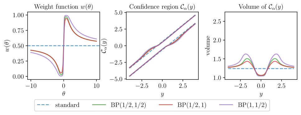
Figure 2: Comparison of the standard and FAB procedures under the Gaussian scale mixture prior with mixing measure $\mathrm{BP}(1/2,1/2)$, $\mathrm{BP}(1/2,1)$ and $\mathrm{BP}(1,1/2)$, respectively, when $Y\mid\theta\sim\mathcal{N}(\theta,0.1)$. All priors result in CRs that are shorter than the standard one when $y$ is close to zero, and that revert to the standard one as $|y|$ increases.

As expected, all FAB-CRs achieve smaller volume than the standard CI when $y$ is close to zero. However, contrary to the Gaussian prior in Fig. 1, these priors result in CRs that are uniformly bounded and revert to the standard CI as $|y|$ increases, ensuring robustness.

4 Extension to natural exponential families

In this section, we generalise Theorem 2.1 to the case where the likelihood $f_{\theta}(y)$ belongs to the exponential family. We first recall some background on natural exponential families (NEF); see (Brown, 1986; Wainwright and Jordan, 2008).

Definition 4.1 (Natural Exponential Family).

Let $\nu$ be a sigma-finite measure on the Borel subsets of $\mathbb{R}^{d}$, and $h:\mathbb{R}^{d}\to[0,\infty)$. Define

$$\Omega=\left\{\eta\mid\int_{\mathbb{R}^{d}}h(y)e^{\eta^{\top}y}\nu(dy)<\infty\right\}.$$ (19)

For any $\eta\in\Omega$, let

$$\psi(\eta)=\log\left(\int_{\mathbb{R}^{d}}h(y)e^{\eta^{\top}y}\nu(dy)\right)$$ (20)

and define, for any $\eta\in\Omega$,

$$f_{\eta}(y)=h(y)e^{\eta^{\top}y-\psi(\eta)}.$$ (21)

The family $\{f_{\eta}(y);\eta\in\Omega\}$ is a $d$-dimensional natural exponential family (NEF) of probability densities with respect to the reference measure $\nu$.

$\Omega$ is called the natural parameter space. We will be interested here in cases where $\Omega$ is an open set. The exponential family is then said to be regular. The reference measure $\nu$ will typically be either the Lebesgue measure or the counting measure. Let $\mathcal{Y}\subseteq\mathbb{R}^{d}$ be the support of $h(y)\nu(dy)$, and let $\mathcal{M}\subseteq\mathbb{R}^{d}$ denote the closure of the convex hull of $\mathcal{Y}$. We will also assume here that the exponential family is minimal, that is $\dim\Omega=\dim\mathcal{M}=d$.

Proposition 4.1 (Mean).

(Wainwright and Jordan, 2008, Section 3.5, Propositions 2 and 3) The set $\Omega$ is a convex set, and $\psi$ is a strictly convex function on $\Omega$. For any $\eta\in\Omega$,

$$\mathbb{E}[Y\mid\eta] =\nabla\psi(\eta)$$ (22)

Moreover, the gradient mapping $\nabla\psi:\Omega\to\mathcal{M}$ is one-to-one.

Assumption 4.1.

Let $\pi(d\eta)$ be a non-degenerate Borel measure on $\Omega$, such that $\pi(A)<\infty$ for any Borel set $A$ of $\Omega$, and $0<\int_{\Omega}f_{\eta}(y)\pi(d\eta)<\infty$ for any $y\in\mathcal{Y}$. We will refer to $\pi$ as the prior distribution on the natural parameter $\eta$. Assume $\pi(d\eta)$ is absolutely continuous w.r.t. some sigma-finite reference measure $\xi$ on $\mathbb{R}^{d}$, with density $g(\eta)$. Let $\widetilde{\Omega}$ be the support of $\pi$, and assume that its closure has dimension $d$. Finally, assume that

$$\widetilde{\mathcal{Y}}=\left\{y\in\mathbb{R}^{d}\mid\int_{\mathbb{R}^{d}}e^{\eta^{\top}y-\psi(\eta)}g(\eta)\xi(d\eta)<\infty\right\}$$ (23)

is an open set.

Remark 4.1.

As in Section 2, $\pi$ will generally be a proper probability distribution, but the definition allows for the use of improper priors. $\xi$ will generally be the Lebesgue measure, but the definition allows for the use of spike and slab priors. Also, in practice one would define a prior on the mean $\nabla\psi(\eta)$, and $\pi$ would be its push-forward measure w.r.t. the inverse gradient map.

Note that $\mathcal{Y}\subseteq\widetilde{\mathcal{Y}}$, hence $\dim(\widetilde{\mathcal{Y}})=d$. For any $y\in\widetilde{\mathcal{Y}}$, let

$$\lambda(y)=\log\left(\int_{\mathbb{R}^{d}}e^{\eta^{\top}y-\psi(\eta)}g(\eta)\xi(d\eta)\right).$$ (24)

For any $y\in\widetilde{Y}$, and any $\eta\in\Omega$, define

$$\widetilde{f}_{y}(\eta)=\left[g(\eta)e^{-\psi(\eta)}\right]e^{\eta^{\top}y-\lambda(y)}.$$ (25)

Then, by definition, the family $\{\widetilde{f}_{y}(\eta);y\in\widetilde{\mathcal{Y}}\}$ defines a regular, minimal, NEF of probability densities over $\Omega$ with respect to the reference measure $\xi$, whose cumulant function is $\lambda(y)$.

Remark 4.2.

For $y\in\mathcal{Y}$, $\widetilde{f}_{y}(\eta)$ may be interpreted as the posterior density of $\eta$ given $y$ under the likelihood $f_{\eta}(y)$ and the prior $\pi$. Similarly, $\lambda(y)$ may be interpreted as $\log\left(\frac{f(y)}{h(y)}\right)$ where $f(y)=\int f_{\eta}(y)g(\eta)\xi(d\eta)$ is the marginal likelihood. The log-ratio between the marginal and the likelihood takes the form $\log\frac{f(y)}{f_{\eta}(y)}=\lambda(y)-\eta^{\top}y+\log(\psi(\eta))$.

We now define the FAB-CR for the natural parameter and for any one-to-one statistical functional of a random variable in the natural exponential family. The procedure below is equivalent to the general FAB procedure described in Section 1, with two differences. To deal in particular with discrete observations, the exact coverage (1) is replaced by a lower bound and, in order to derive the focal point, the log-likelihood function is extended on the larger (convex) space $\widetilde{\mathcal{Y}}\supseteq\mathcal{Y}$.

Definition 4.2.

Let $\alpha\in(0,1)$ and $Y\sim f_{\eta}$ be a random variable in the regular, minimal NEF with cumulant $\psi$. Let $\theta=\mathcal{F}(\eta)$ be some one-to-one statistical functional of the density $f_{\eta}$ e.g. its mean, median or quantile. In the case of the mean, $\mathcal{F}=\nabla\psi$. Let $g(\eta)$ be some prior density on the natural parameter $\eta$ with respect to some reference measure $\xi$. For any $y\in\widetilde{\mathcal{Y}}$, let

$$\lambda_{\eta}(y)=\lambda(y)-\eta^{\top}y+\log(\psi(\eta)).$$ (26)

The $(1-\alpha)$ FAB-CR $C_{\alpha}(y)$ for the parameter $\theta$ is

$$C_{\alpha}(y)=\{\mathcal{F}(\eta)\mid\eta\in C_{\alpha}^{\mathrm{np}}(y)\}$$ (27)

where $C_{\alpha}^{\mathrm{np}}$ is the $(1-\alpha)$ FAB-CR for the natural parameter $\eta$, defined as

$$C_{\alpha}^{\mathrm{np}}(y)=\{\eta\in\Omega\mid y\in A_{\alpha}^{\mathrm{np}}(\eta)\}$$

with

$$A_{\alpha}^{\mathrm{np}}(\eta)=\left\{y\in\widetilde{\mathcal{Y}}\mid\lambda_{\eta}(y)\leq k_{\alpha}(\eta)\right\}$$ (28)

where $k_{\alpha}(\eta)$ is the smallest value such that

$$\int_{A_{\alpha}^{\mathrm{np}}(\eta)}f_{\eta}(y)\nu(dy)\geq 1-\alpha.$$

For discrete observations, $\lim_{\alpha\to 1}\mathrm{vol}(C_{\alpha}(y))\neq 0$, and $\cap_{\alpha\in(0,1)}C_{\alpha}$ is therefore an interval, preventing the use of (6) as a focal point. We use instead the following definition for the focal point

$$\widehat{\eta}^{\mathrm{FAB}}(y)=y_{\min}^{-1}(y)$$

where

$$y_{\min}(\eta)=\arg\min_{y\in\widetilde{\mathcal{Y}}}\lambda_{\eta}(y)$$

and

$$\widehat{\theta}^{\mathrm{FAB}}(y)=\mathcal{F}(\widehat{\eta}^{\mathrm{FAB}}(y)).$$

The above definition reduces to (6) if $\lim_{\alpha\to 1}\mathrm{vol}(C_{\alpha}(y))=0$.

For any $y\in\widetilde{\mathcal{Y}}$, let

$$\widehat{\eta}(y)=\int\eta\widetilde{f}_{y}(\eta)\xi(d\eta)=\nabla\lambda(y)$$ (29)

be the mean of the random variable with density (25). If $y\in\mathcal{Y}\subseteq\widetilde{\mathcal{Y}}$, then $\widehat{\eta}(y)=\mathbb{E}[\eta\mid y]$ is the posterior mean of the natural parameter $\eta$ given $y$ under the likelihood $f_{\eta}(y)$ and prior $\pi$. The next proposition shows that, when constructing a FAB-CR $C_{\alpha}(y)$ for the natural parameter $\eta$, its posterior mean $\mathbb{E}[\eta\mid y]$ always lies in the confidence interval.

Theorem 4.1.

Assume that 4.1 holds. Let $\alpha\in(0,1)$. For any $\eta\in\Omega$, $A_{\alpha}^{\mathrm{np}}(\eta)$ is a convex set, and $\widehat{\eta}^{-1}(\eta)\in A_{\alpha}^{\mathrm{np}}(\eta)$. For an observation $y\in\mathcal{Y}$, let $C_{\alpha}(y)$ and $C_{\alpha}^{\mathrm{np}}(y)$ be the $(1-\alpha)$ FAB-CR for $\theta$ and $\eta$, respectively, as defined in Definition 4.2. Then,

$$\widehat{\eta}^{\mathrm{FAB}}=\nabla\lambda(y)=\mathbb{E}[\eta\mid y]\in C_{\alpha}^{\mathrm{np}}(y)$$ (30)

and

$$\widehat{\theta}^{\mathrm{FAB}}=\mathcal{F}(\nabla\lambda(y))=\mathcal{F}(\mathbb{E}[\eta\mid y])\in C_{\alpha}(y).$$ (31)

Proof.

Note that $\lambda_{\eta}(y)$ is a strictly convex function. $A_{\alpha}^{\mathrm{np}}$ is a sublevel set of $\lambda_{\eta}$, and is therefore convex. $\lambda_{\eta}$ is differentiable w.r.t. $y$, with

$$\nabla\lambda_{\eta}(y)=\nabla\lambda(y)-\eta.$$

Solving $\nabla\lambda_{\eta}(y)=0$ gives $y=(\nabla\lambda)^{-1}(\eta)$. Hence $(\nabla\lambda)^{-1}(\eta)\in A_{\alpha}^{\mathrm{np}}(\eta)$, therefore $\nabla\lambda(y)\in C_{\alpha}^{\mathrm{np}}(y)$. It follows that $\mathcal{F}(\nabla\lambda(y))\in C_{\alpha}(y)$. ∎

Example 4.1.

Let $Y\sim\mathrm{Binomial}(n,p)$ be a Binomial random variable with mean $\theta=np$. It takes the NEF form $f_{\eta}(y)=e^{\eta y-\psi(\eta)}$ where $\eta=\log(\theta/(n-\theta))\in\mathbb{R}$, $\psi(\eta)=n\log(1+e^{\eta})$ and $h(y)=\left(\begin{array}[]{c}n\\ y\\ \end{array}\right)$. Assuming $\theta\sim\mathrm{Beta}(a,b)$, $\eta=\log(\theta/(n-\theta))$ follows a logistic-beta distribution, with density $g(\eta)$. We have

$$\lambda(y) =\log\int e^{\eta y-\psi(\eta)}g(\eta)d\eta$$ (32)

$$=\log\frac{B(a+y,b+n-y)}{B(a,b)}$$ (33)

$$=\log\frac{\Gamma(a+y)\Gamma(b+n-y)\Gamma(a+b)}{\Gamma(a+b+n)\Gamma(a)\Gamma(b)}$$ (34)

which is defined for $y\in\widetilde{\mathcal{Y}}=(-a,b+n)$. Its derivative is

$$\lambda^{\prime}(y)=\mathrm{di}\Gamma(a+y)-\mathrm{di}\Gamma(b+n-y)=\widehat{\eta}(y),$$

where $\mathrm{di}\Gamma(z)$ is the digamma function. For $y\in\{0,1\}$, $\lambda^{\prime}(y)=\mathbb{E}[\eta\mid y]\in C_{\alpha}^{\mathrm{np}}(y)$. Similarly, $\psi^{\prime}(\eta)=\frac{n}{1+e^{-\eta}}$, hence $n(1+e^{-(\mathrm{di}\Gamma(a+y)-\mathrm{di}\Gamma(b+n-y))})^{-1}\in C_{\alpha}(y)$. When using a uniform prior ($a=b=1$), one recovers the intervals for binomial proportions introduced by Sterne (1954); see also (Crow, 1956) and the discussion in (Pratt, 1961, Section 6). The construction can be generalised to multinomial random variables. When using a uniform prior over the simplex (Dirichlet prior with parameters equal to 1), one recovers the confidence regions of Chafai and Concordet (2009) and Malloy et al. (2020).

Example 4.2.

Let $Y$ be a Poisson random variable with mean $\theta$. It takes the NEF form $f_{\eta}(y)=h(y)e^{\eta y-\psi(\eta)}$ where $\eta=\log(\theta)\in\mathbb{R}$, $\psi(\eta)=e^{\eta}$ and $h(y)=1/y!$. Assume $\theta\sim\mathrm{Gamma}(a,p/(1-p))$, then $\eta$ follows a log-gamma distribution, and

$$\lambda(y) =\log\int e^{\eta y-\psi(\eta)}g(\eta)d\eta$$ (35)

$$=\log\left(\frac{\Gamma(a+y)}{\Gamma(a)}(1-p)^{y}p^{a}\right)$$ (36)

We obtain

$$\lambda^{\prime}(y) =\mathrm{di}\Gamma(a+y)+\log(1-p)$$ (37)

When $y\in\mathbb{N}$, this corresponds to $\mathbb{E}[\eta\mid y]$ (expectation of log of gamma RV with parameters $(a+y,p/(1-p)+1)$). Additionally, $\psi^{\prime}(\eta)=e^{\eta}$, hence $\exp(\mathrm{di}\Gamma(a+y)+\log(1-p))=(1-p)e^{\mathrm{di}\Gamma(a+y)}$ always belongs to the FAB-CR for the mean parameter $\theta$.

Appendix A Proofs

A.1 Proof of Lemma 2.1

Proof.

For ease of presentation, we drop the subscript $\alpha$ and write $w$ for $w_{\alpha}$. We prove that $w(\theta)$ is bounded away from 0 and converges to 1/2 as $\theta\to-\infty$. The proof that it is bounded away from 1 and converges to 1/2 as $\theta\to\infty$ proceeds similarly. Let $\alpha<\frac{1}{2}$. Let $\mu_{1}(w)=z_{1-\alpha(1-w)}$ and $\mu_{2}(w)=z_{1-\alpha w}$, which take values in $[z_{1-\alpha},\infty)$. Assume for a contradiction that $w(\theta)$ is not bounded away from 0. Let $(w_{n})_{n\geq 1}$ be a sequence in $(0,1)$ such that $w_{n}<\frac{1-\Phi(n)}{\alpha}$ for all $n\geq 1$. Then, $\mu_{1}(w_{n})\in[z_{1-\alpha},z_{2-\alpha-\Phi(n)}]$ and$\ \mu_{2}(w_{n})>n$. For $n\geq 1$, let $\theta_{n}$ be the solution of $\lambda_{\theta_{n}}(\theta_{n}+\mu_{1}(w_{n}))=\lambda_{\theta_{n}}(\theta_{n}-\mu_{2}(w_{n}))$ or, equivalently,

$$f\left(\theta_{n}+\mu_{1}(w_{n})\right)\exp\left(\frac{1}{2}\left[\mu_{1}(w_{n})\right]^{2}\right)=f\left(\theta_{n}-\mu_{2}(w_{n})\right)\exp\left(\frac{1}{2}\left[\mu_{2}(w_{n})\right]^{2}\right).$$

As Eq. 13 holds, $f(y)\leq M$ on $\mathbb{R}$ and

$$f\left(\theta_{n}+\mu_{1}(w_{n})\right)\exp\left(\frac{1}{2}\left[\mu_{1}(w_{n})\right]^{2}\right)\leq M\exp\left(\frac{1}{2}\left[z_{2-\alpha-\Phi(n)}\right]^{2}\right).$$

Hence, for any $\varepsilon>0$, and any $n$ large enough,

$$f\left(\theta_{n}-\mu_{2}(w_{n})\right) \leq M\exp\left(\frac{1}{2}\left[\mu_{1}(w_{n})\right]^{2}\right)\exp\left(-\frac{1}{2}\left[\mu_{2}(w_{n})\right]^{2}\right)$$ (38)

$$\leq M\exp\left(\frac{1}{2}\left[z_{1-\alpha}+\varepsilon\right]^{2}\right)\exp\left(-\frac{1}{2}n^{2}\right).$$

By sandwiching, $f\left(\theta_{n}-\mu_{2}(w_{n})\right)\rightarrow 0$ as $n\rightarrow\infty$. If $\delta=0$, this leads to a contradiction; hence, $\delta>0$ and $\left|\theta_{n}-\mu_{2}(w_{n})\right|\rightarrow\infty$. From Eq. 13, we have $f\left(\theta_{n}-\mu_{2}(w_{n})\right)\sim\gamma\left|\theta_{n}-\mu_{2}(w_{n})\right|^{-\delta}$. From Eq. 38, $f\left(\theta_{n}-\mu_{2}(w_{n})\right)=O(\exp\left(-\frac{1}{2}\left[\mu_{2}(w_{n})\right]^{2}\right))$; this implies $|\mu_{2}(w_{n})|=o(|\theta_{n}|)$. Hence, $|\theta_{n}-\mu_{2}(w_{n})|\sim|\theta_{n}|\sim\gamma|\theta_{n}|^{-\delta}$. Additionally, as $\mu_{1}(w_{n})$ is bounded, $|\theta_{n}-\mu_{1}(w_{n})|\sim|\theta_{n}|$ as $n\to\infty$, and $f(\theta_{n}-\mu_{1}(w_{n}))\sim\gamma|\theta_{n}|^{-\delta}$ as $n\to\infty$. It follows that

$$\frac{f\left(\theta_{n}+\mu_{1}(w_{n})\right)}{f\left(\theta_{n}-\mu_{2}(w_{n})\right)}\rightarrow 1\text{ as }n\rightarrow\infty,$$

hence for any $\varepsilon_{2}>0$, there is $N$ large enough such that for all $n\geq N,$

$$e^{n/2}\leq\exp\left(\frac{1}{2}\left[\mu_{2}(w_{n})\right]^{2}\right)=\frac{f\left(\theta_{n}+\mu_{1}(w_{n})\right)}{f\left(\theta_{n}-\mu_{2}(w_{n})\right)}\exp\left(\frac{1}{2}\left[\mu_{1}(w_{n})\right]^{2}\right)\leq\exp(\frac{1}{2}(z_{1-\alpha})^{2})+\varepsilon_{2}.$$

Taking $n\geq N$ large enough gives the required contradiction. Henc,e $w$ is bounded away from 0. The proof for 1 proceeds similarly.

We now prove $w(\theta)\to 1/2$ as $\theta\to\infty$. As $w$ if bounded away from $0$ and $1$, the functions $z_{\alpha(1-w(\cdot))}$ and $z_{1-\alpha w(\cdot)}$ are bounded. Then $\left|\theta-z_{\alpha(1-w)}\right|\sim\left|\theta-z_{1-\alpha w}\right|\sim|\theta|$ as $\theta\rightarrow\infty$. It follows from (13) that

$$\lim_{\theta\rightarrow\infty}\frac{f\left(\theta-z_{\alpha(1-w)}\right)}{f\left(\theta-z_{1-\alpha w}\right)}=1$$

hence, for any $\delta>0$, there exists $\theta$ large enough such that $w(\theta)$ satisfies

$$1-\delta\leq\frac{\exp\left(-\frac{1}{2}\left[z_{\alpha(1-w)}\right]^{2}\right)}{\exp\left(-\frac{1}{2}\left[z_{1-\alpha w}\right]^{2}\right)}\leq 1+\delta$$

The function $h(w)=\frac{\exp\left(-\frac{1}{2}\left[z_{\alpha(1-w)}\right]^{2}\right)}{\exp\left(-\frac{1}{2}\left[z_{1-\alpha w}\right]^{2}\right)}$ is continuous, strictly monotone from $(0,1)$ into $(0,\infty)$, therefore has a continuous inverse $h^{-1}$. By continuity of $h^{-1}$, for any $\varepsilon>0$, there exists $\delta>0$ such that $\left|h(w)-1\right|$$<$$\delta$ implies $\left|w-h^{-1}(1)\right|=\left|w-1/2\right|<\varepsilon$. This completes the proof. ∎

A.2 Proof of Proposition 3.1

Proof.

The marginal likelihood $f(y;\sigma)$ under the prior $\pi(\theta;\sigma)$ is given by

$$f(y;\sigma) =\int_{\mathbb{R}}f_{\theta}(y)\pi(\theta;\sigma)d\theta$$

$$=\int_{\mathbb{R}}f_{\theta}(y)\frac{1}{\sigma}\pi\left(\frac{\theta}{\sigma};1\right)d\theta$$

$$=\int_{\mathbb{R}}f_{(\sigma\theta^{\prime})}(y)\pi(\theta^{\prime};1)d\theta^{\prime}$$

$$=\frac{1}{\sigma}\int_{\mathbb{R}}f_{\theta^{\prime}}\left(\frac{y}{\sigma}\right)\pi(\theta^{\prime};1)d\theta^{\prime}$$

$$=\frac{1}{\sigma}f\left(\frac{y}{\sigma};1\right),$$ (39)

where the third equality follows from the change of variables $\theta^{\prime}=\theta/\sigma$. By Eq. 10, $\underline{A}_{\alpha}(\theta;\sigma)$ and $\overline{A}_{\alpha}(\theta;\sigma)$ under the prior $\pi(\theta;\sigma)$ satisfy

$$f(\underline{A}_{\alpha}(\theta;\sigma);\sigma)\exp\left(\frac{\underline{A}_{\alpha}(\theta;\sigma)^{2}}{2\sigma^{2}}\right)=f(\overline{A}_{\alpha}(\theta;\sigma);\sigma)\exp\left(\frac{\overline{A}_{\alpha}(\theta;\sigma)^{2}}{2\sigma^{2}}\right)$$ (40)

under the constraint in Eq. 11. Furthermore, by Eq. 39, Eq. 40 is equivalent to

$$f\left(\frac{\underline{A}_{\alpha}(\theta;\sigma)}{\sigma};1\right)\exp\left(\frac{(\underline{A}_{\alpha}(\theta;\sigma)/\sigma)^{2}}{2}\right)=f\left(\frac{\overline{A}_{\alpha}(\theta;\sigma)}{\sigma};1\right)\exp\left(\frac{(\overline{A}_{\alpha}(\theta;\sigma)/\sigma)^{2}}{2}\right).$$

We have that $\underline{A}_{\alpha}(\theta;\sigma)=\sigma\underline{A}_{\alpha}(\theta/\sigma;1)$ and $\overline{A}_{\alpha}(\theta;\sigma)=\sigma\overline{A}_{\alpha}(\theta/\sigma;1)$. To see this, plug these expressions into Section A.2, which becomes

$$f\left(\underline{A}_{\alpha}(\theta/\sigma;1);1\right)\exp\left(\frac{\underline{A}_{\alpha}(\theta/\sigma;1)^{2}}{2}\right)=f\left(\overline{A}_{\alpha}(\theta/\sigma;1);1\right)\exp\left(\frac{\overline{A}_{\alpha}(\theta;1)^{2}}{2}\right).$$

Similarly, Eq. 11 takes the form

$$\Phi\left(\overline{A}_{\alpha}(\theta/\sigma;1)-\frac{\theta}{\sigma}\right)-\Phi\left(\underline{A}_{\alpha}(\theta/\sigma;1)-\frac{\theta}{\sigma}\right)=1-\alpha.$$

Finally, by plugging in the expressions for $\underline{A}_{\alpha}(\theta;\sigma)$ into Eq. 8, we obtain

$$w_{\alpha}(\theta;\sigma) =\frac{1}{\alpha}\Phi\left(\underline{A}_{\alpha}(\theta/\sigma;1)-\frac{\theta}{\sigma}\right)=w_{\alpha}(\theta/\sigma;1),$$

as desired. From now on, we suppress the scale parameter $\sigma$ in the notation to indicate $\sigma=1$. If $\pi(\theta)$ is symmetric about $0$, then also $f(y)$ is, since

$$f(-y)=\int_{\mathbb{R}}f_{\theta}(-y)\pi(\theta)d\theta=\int_{\mathbb{R}}f_{-\theta}(y)\pi(\theta)d\theta=f(y).$$

This implies that $\underline{A}_{\alpha}(-\theta)=-\overline{A}_{\alpha}(\theta)$ and $\overline{A}_{\alpha}(-\theta)=-\underline{A}_{\alpha}(\theta)$. To see this, notice that these expressions for $\underline{A}_{\alpha}(-\theta)$ and $\overline{A}_{\alpha}(-\theta)$ satisfy Eq. 10 and, moreover, Eq. 11 becomes

$$\Phi\left(\overline{A}_{\alpha}(-\theta)+\theta\right)-\Phi\left(\underline{A}_{\alpha}(-\theta)+\theta\right) =\Phi\left(-\underline{A}_{\alpha}(\theta)+\theta\right)-\Phi\left(-\overline{A}_{\alpha}(\theta)+\theta\right)=1-\alpha$$

because $\Phi(-x)=1-\Phi(x)$. By plugging in the expression for $\underline{A}_{\alpha}(-\theta)$ into Eq. 8 and using the expression for $\overline{A}_{\alpha}(\theta)$ in Eq. 9, this implies that

$$w_{\alpha}(-\theta)=\frac{1}{\alpha}\Phi\left(-\overline{A}_{\alpha}(\theta)+\theta\right)=\frac{1}{\alpha}\Phi\left(-\Phi^{-1}\left(1-\alpha(1-w_{\alpha}(\theta))\right)\right)=1-w_{\alpha}(\theta),$$

as desired. ∎

A.3 Proof of Proposition 3.2

Proof.

The marginal likelihood $f(y)$ is given by

$$f(y) =\int_{\mathbb{R}}f_{\theta}(y)\pi(\theta)d\theta$$

$$=\int_{\mathbb{R}}\mathcal{N}(y;\theta,\sigma^{2})\left(\int_{0}^{\infty}\mathcal{N}(\theta;0,\sigma^{2}\tau^{2})f_{\tau^{2}}(\tau^{2})d\tau^{2}\right)d\theta$$

$$=\int_{0}^{\infty}\mathcal{N}(y;0,\sigma^{2}(1+\tau^{2}))f_{\tau^{2}}(\tau^{2})d\tau^{2}$$

$$=\frac{1}{\sqrt{2\pi\sigma^{2}}}\int_{0}^{\infty}\frac{1}{\sqrt{1+\tau^{2}}}\exp\left(-\frac{y^{2}}{2\sigma^{2}(1+\tau^{2})}\right)f_{\tau^{2}}(\tau^{2})d\tau^{2}.$$

Using the change of variable $u=1/(1+\tau^{2})$, this becomes

$$f(y) =\frac{1}{\sqrt{2\pi\sigma^{2}}}\int_{0}^{1}\exp\left(-u\frac{y^{2}}{2\sigma^{2}}\right)u^{-3/2}f_{\tau^{2}}\left(\frac{1-u}{u}\right)du$$ (41)

$$=g\left(\frac{y^{2}}{2\sigma^{2}}\right),$$

where

$$g(x)=\int_{0}^{1}\frac{1}{\sqrt{2\pi\sigma^{2}}}e^{-ux}u^{-3/2}f_{\tau^{2}}\left(\frac{1-u}{u}\right)du.$$

Since $f_{\tau^{2}}(\tau^{2})\sim C_{1}(\tau^{2})^{-(\beta+1)}$ as $\tau^{2}\to\infty$, we have

$$\frac{1}{\sqrt{2\pi\sigma^{2}}}u^{-3/2}f_{\tau^{2}}\left(\frac{1-u}{u}\right)\sim\frac{C_{1}}{\sqrt{2\pi\sigma^{2}}}u^{-3/2}u^{\beta+1}$$

as $u\to 0$. By Karamata’s Tauberian theorem on regularly varying functions (Bingham et al., 1989, Theorem 1.7.1’), this implies

$$g(x)\sim\frac{C_{1}}{\sqrt{2\pi\sigma^{2}}}\frac{\Gamma(\beta+1/2)}{x^{\beta+1/2}}$$

as $x\to\infty$. Finally, from standard properties of regularly varying functions, we have that

$$f(y)\sim C_{1}\frac{(2\sigma^{2})^{\beta}}{\sqrt{\pi}}\Gamma(\beta+1/2)|y|^{-(2\beta+1)}$$

as $y\to\pm\infty$, as desired. ∎

A.4 Proof of Proposition 3.3

Proof.

Starting from the same change of variables as in Eq. 41, the marginal likelihood $f(y)$ is given by

$$f(y) =\frac{1}{\sqrt{2\pi\sigma^{2}}}\int_{0}^{1}\exp\left(-u\frac{y^{2}}{2\sigma^{2}}\right)u^{-3/2}f_{\tau^{2}}\left(\frac{1-u}{u}\right)du$$

$$=\frac{1}{B(a,b)\sqrt{2\pi\sigma^{2}}}\int_{0}^{1}\exp\left(-u\frac{y^{2}}{2\sigma^{2}}\right)u^{-3/2}\left(\frac{1-u}{u}\right)^{b-1}\left(\frac{1}{u}\right)^{-(a+b)}du$$

$$=\frac{1}{B(a,b)\sqrt{2\pi\sigma^{2}}}\int_{0}^{1}\exp\left(-u\frac{y^{2}}{2\sigma^{2}}\right)u^{a-1/2}(1-u)^{b-1}du$$

$$=\frac{1}{B(a,b)\sqrt{2\pi\sigma^{2}}}\times\frac{\Gamma(b)\Gamma(a+1/2)}{\Gamma(a+b+1/2)}\times{{}_{1}F_{1}}\left(a+1/2,a+b+1/2,-\frac{y^{2}}{2\sigma^{2}}\right)$$

$$=\frac{1}{\sqrt{2\pi\sigma^{2}}}\times\frac{\Gamma(a+b)\Gamma(a+1/2)}{\Gamma(a+b+1/2)\Gamma(a)}\times{{}_{1}F_{1}}\left(a+1/2,a+b+1/2,-\frac{y^{2}}{2\sigma^{2}}\right)$$

because ${}_{1}F_{1}(\alpha,\beta,z)$ admits integral representation (Abramowitz and Stegun, 1968)

$${}_{1}F_{1}(\alpha,\beta,z)=\frac{\Gamma(\beta)}{\Gamma(\beta-\alpha)\Gamma(\alpha)}\int_{0}^{1}e^{zu}u^{\alpha-1}(1-u)^{\beta-\alpha-1}du.$$

Moreover, $f^{\prime}(y)$ is given by

$$f^{\prime}(y)=-\frac{1}{\sqrt{2\pi\sigma^{2}}}\times\frac{\Gamma(a+b)\Gamma(a+3/2)}{\Gamma(a+b+3/2)\Gamma(a)}\times\frac{y}{\sigma^{2}}\times{{}_{1}F_{1}}\left(a+3/2,a+b+3/2,-\frac{y^{2}}{2\sigma^{2}}\right)$$

because

$$\frac{\partial}{\partial z}{{}_{1}F_{1}}(\alpha,\beta,z)=\frac{\alpha}{\beta}{{}_{1}F_{1}}(\alpha+1,\beta+1,z).$$

As a result of this, by Tweedie’s formula (7),

$$\mathbb{E}[\theta|y]=y+\sigma^{2}\frac{f^{\prime}(y)}{f(y)},$$

from which the expression for $\widehat{\theta}^{\text{FAB}}(y)$ follows. ∎

References

• Abramowitz and Stegun (1968) Abramowitz, M. and I.Β A. Stegun (1968). Handbook of mathematical functions with formulas, graphs, and mathematical tables, VolumeΒ 55. US Government printing office.
• Andrews and Mallows (1974) Andrews, D. and C.Β Mallows (1974). Scale mixtures of normal distributions. Journal of the Royal Statistical Society: Series B (Methodological)Β 36(1), 99–102.
• Armagan etΒ al. (2011) Armagan, A., D.Β B. Dunson, and M.Β Clyde (2011). Generalized Beta Mixtures of Gaussians. Advances in neural information processing systemsΒ 24, 523.
• Bingham etΒ al. (1989) Bingham, N.Β H., C.Β M. Goldie, and J.Β L. Teugels (1989). Regular variation, VolumeΒ 27. Cambridge university press.
• Brown (1986) Brown, L.Β D. (1986). Fundamentals of Statistical Exponential Families with Applications in Statistical Decision Theory. Lecture Notes-Monograph SeriesΒ 9, i–279. Publisher: Institute of Mathematical Statistics.
• Brown etΒ al. (1995) Brown, L.Β D., G.Β Casella, and J.Β G.Β Hwang (1995). Optimal confidence sets, bioequivalence, and the limacon of Pascal. Journal of the American Statistical AssociationΒ 90(431), 880–889.
• Carvalho etΒ al. (2010) Carvalho, C.Β M., N.Β G. Polson, and J.Β G. Scott (2010). The horseshoe estimator for sparse signals. BiometrikaΒ 97(2), 465–480.
• Chafai and Concordet (2009) Chafai, D. and D.Β Concordet (2009). Confidence regions for the multinomial parameter with small sample size. Journal of the American Statistical AssociationΒ 104(487), 1071–1079.
• Crow (1956) Crow, E.Β L. (1956). Confidence intervals for a proportion. BiometrikaΒ 43(3/4), 423–435.