AdaNeg: Adaptive Negative Proxy Guided
OOD Detection with Vision-Language Models
Abstract
Recent research has shown that pre-trained vision-language models are effective at identifying out-of-distribution (OOD) samples by using negative labels as guidance. However, employing consistent negative labels across different OOD datasets often results in semantic misalignments, as these text labels may not accurately reflect the actual space of OOD images. To overcome this issue, we introduce adaptive negative proxies, which are dynamically generated during testing by exploring actual OOD images, to align more closely with the underlying OOD label space and enhance the efficacy of negative proxy guidance. Specifically, our approach utilizes a feature memory bank to selectively cache discriminative features from test images, representing the targeted OOD distribution. This facilitates the creation of proxies that can better align with specific OOD datasets. While task-adaptive proxies average features to reflect the unique characteristics of each dataset, the sample-adaptive proxies weight features based on their similarity to individual test samples, exploring detailed sample-level nuances. The final score for identifying OOD samples integrates static negative labels with our proposed adaptive proxies, effectively combining textual and visual knowledge for enhanced performance. Our method is training-free and annotation-free, and it maintains fast testing speed. Extensive experiments across various benchmarks demonstrate the effectiveness of our approach, abbreviated as AdaNeg. Notably, on the large-scale ImageNet benchmark, our AdaNeg significantly outperforms existing methods, with a 2.45% increase in AUROC and a 6.48% reduction in FPR95. Codes are available at https://github.com/YBZh/OpenOOD-VLM.
1 Introduction
In real applications, artificial intelligence (AI) systems often encounter test samples of unknown classes, termed out-of-distribution (OOD) data. These OOD data often result in overly confident errors [52, 44], posing security threats. Therefore, accurately identifying OOD data is essential for ensuring the reliability and security of AI systems in open-world environments.
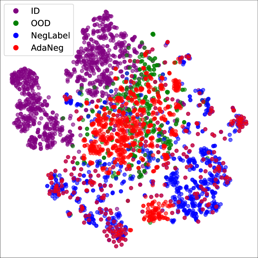
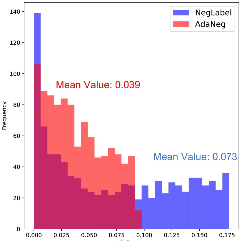
Traditional OOD detection methods in image domain primarily rely on vision-only models [20, 33, 36]. Recent advancements in vision-language models (VLMs) have demonstrated remarkable OOD detection performance by leveraging multi-modal knowledge [17, 15, 39]. Recently, NegLabel [27] explores negative labels by identifying text labels that are semantically distant from the in-distribution (ID) labels. This method achieves state-of-the-art performance by detecting test images closer to negative labels as OOD. In other words, NegLabel regards these negative labels as proxies of OOD data. However, employing consistent negative labels across different OOD datasets often leads to semantic misalignment, where these text labels may not accurately reflect the actual label space of OOD images, as shown in Fig. 1. This misalignment between the proxies and targeted OOD distribution leads to sub-optimal performance.
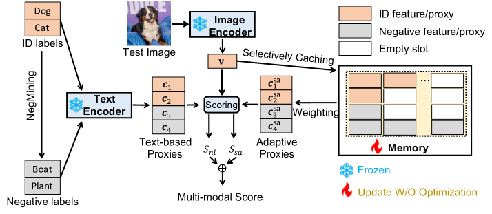
To promote the alignment between the negative proxies and target OOD distribution, we introduce the Adaptive Negative proxies (AdaNeg), which are dynamically generated during testing by exploring actual OOD images. Specifically, we start by initializing an empty category-split memory bank for each OOD dataset and selectively cache features of discriminative OOD images during testing. The OOD discrimination is assessed using mined negative labels, as detailed in [27]. With this feature memory, we develop task-adaptive proxies by simply averaging cached features within each category. These proxies, derived from actual OOD images, reflect the distinct characteristics of the target OOD dataset and align more closely with the underlying OOD label space.
The task-adaptive proxies mentioned previously provide unique proxies for different OOD datasets while maintaining consistency across various test samples within the same dataset. To delve into the fine-grained nuances at the sample level, we introduce the sample-adaptive proxies by weighting cached features based on their similarity to a particular test sample. This is achieved with an attention mechanism, where the feature memory serves as both keys and values, and the test feature acts as the query. The final score for detecting OOD samples integrates static negative labels with our adaptive proxies, effectively combining textual and visual knowledge for enhanced performance.
We conduct extensive experiments on standard benchmarks to validate the effectiveness of AdaNeg, where our proposed adaptive proxies outperform the negative-label-based one, enhancing performance with complementary multi-modal knowledge. Particularly, on the large-scale ImageNet dataset, our AdaNeg method outperforms existing methods by 2.45% AUROC and 6.48% FPR95. Notably, our method is training-free and annotation-free, and it maintains fast testing speed, as analyzed in Tab. 4. The ability to dynamically adjust to new OOD datasets without affecting testing speed or labor-intensive annotation/training makes our approach particularly valuable for real-world applications where adaptability and efficiency are crucial. We summarize our contribution as follows:
-
•
We first identify the label space misalignment between existing negative-label-based proxies and the target OOD distributions. In response, we introduce adaptive negative proxies that are dynamically generated during testing by exploring actual OOD images, resulting in a more effective alignment with the OOD label space.
-
•
Our adaptive negative proxies are constructed with a feature memory bank that selectively caches discriminative image features during testing. We instantiate this concept by developing task-adaptive proxies to reflect the unique characteristics of each OOD dataset and sample-adaptive proxies to capture detailed sample-level nuances. The final OOD detection score combines these insights with complementary textual and visual knowledge.
-
•
We conduct thorough analyses of the proposed components and perform extensive experiments on standard benchmarks. Our method is training-free and annotation-free, and it maintains fast testing speed and achieves state-of-the-art performance. Notably, our method significantly outperforms existing methods, with a 2.54% increase in AUROC and a 6.48% reduction in FPR95 on the large-scale ImageNet dataset.
2 Related Work
OOD Detection focuses on identifying OOD test samples with semantic shifts, thus distinguishing it from generalization studies which typically focus on covariate shifts [3, 4, 5, 75]. A variety of OOD detection techniques have been developed, which can be roughly categorized into score-based [20, 33, 36, 37, 66, 26, 64, 56], distance-based [58, 59, 57, 12, 41, 53], and generative-based [50, 29] methods. Among them, score-based methods are particularly notable by employing a variety of scoring functions to differentiate between ID and OOD samples. These functions include confidence-based [20, 36, 56, 64], discriminator-based [29], energy-based [37, 66], and gradient-based [25] scores. In contrast, distance-based methods determine OOD samples by evaluating the distance in the feature space between test data and the closest ID samples [58] or ID prototypes [59], using metrics such as KNN [57, 12, 41] or Mahalanobis distance [33, 53].
Despite their achievements, traditional OOD detection methods generally rely on manually annotated ID images and often overlook the integration of textual information. To leverage the textual knowledge, recent advancements have focused on employing VLMs [39, 40, 27, 77, 76, 15, 42, 65, 45]. Specifically, ZOC [15] applies VLMs to discern OOD instances by training a captioner that generates potential OOD labels. Nevertheless, this captioner often fails to produce effective OOD labels, particularly for ID datasets containing many classes. LoCoOp [42] adopts a novel approach by learning ID prompts from few-shot ID samples, and further enhances the robustness of these prompts by incorporating OOD features mined from the backgrounds of images. CLIPN [65], LSN [45] and LAPT [76] explore learning text prompts for expressing negative concepts. In specific, CLIPN initializes text prompts with the word ‘no’ combined with ID labels and refines them with large-scale multi-modal data; LSN starts with manually collected ID samples to learn negative prompts, offering a different approach to leveraging textual information in OOD detection; LAPT conducts automated prompt tuning with automatically collected training samples, boosting OOD detection without any manual effort. MCM [39] utilizes ID class names to facilitate effective zero-shot OOD detection. It is further refined by NegLabel [27], which incorporates additional negative class names mined from available data sources as negative proxies. However, as illustrated in Fig. 1, there is a mismatch between the negative-label-based proxies and the target OOD distribution, underscoring the limitations of this strategy. This observation has inspired us to construct adaptive proxies by exploring potential OOD test images during testing. This leads to an efficient method that aligns better with the target OOD distribution, resulting in enhanced OOD detection performance.
Furthermore, we clarify the relationship between our method and existing approaches on OOD exposure [17, 21, 73]. Most OOD exposure methods introduce manually collected negative images during training, where manual labor is necessary to ensure that the labels of negative images are different from ID ones. Moreover, involving negative images in training typically introduces additional computational overhead, impeding its practical deployment. Unlike these methods, NegLabel [27] is exposed to negative labels during the test phase in a training-free manner. However, given a fixed ID dataset, the exposed negative texts remain consistent for different OOD datasets, inevitably resulting in label misalignment, as shown in Fig. 1. To address this, we expose the VLMs to adaptive negative proxies, which explore actual OOD samples during testing and align more effectively with OOD distribution. Our method does not require manual annotations and works in a training-free manner, making it an appealing solution for real applications.
Test-time Adaptation. We adopt an online update of the negative proxies during testing, resembling test-time adaptation (TTA) methods [35, 63, 54]. Existing TTA methods primarily address covariate shifts between training and testing domains. In contrast, our approach mitigates the label shift between negative proxies and the target OOD distribution by exploring online test samples. Recently, TTA strategies have been considered in the field of OOD detection. However, these methods typically require test-time optimization [18, 72, 16], slowing down the testing process. In contrast, our method is optimization-free and introduces only a lightweight memory interaction operation, enabling rapid and accurate testing, as analyzed in Tab. 4.
Memory Networks. The use of memory networks for storing and retrieving past knowledge [67, 55] has been extensively applied across various fields, including classification [28, 51, 77], segmentation [46, 69], detection [8, 6], and NLP [47]. To our best knowledge, our work is the first to apply memory networks to the field of OOD detection. By caching and retrieving test images with a feature memory, we propose adaptive proxies to more effectively align with the OOD distribution in a training-free manner. This innovative approach significantly enhances the OOD detection performance.
3 Methodology
3.1 Preliminaries
OOD Detection Setup. Consider as the image domain and as the space of ID class labels, where comprises text elements such as , and represents the total number of classes. Let and be random variables representing ID and OOD samples from , respectively. We define and as the marginal distributions for ID and OOD, respectively. In conventional classification scenarios, it is assumed that the test image originates from the ID and is associated with a specific ID label, specifically, and , with being the label of . However, in real applications, AI systems often face data from unknown classes, denoted by and . Such occurrences can make AI models incorrectly categorize these instances into familiar ID categories with substantial certainty [52, 44], resulting in security concerns. To address these challenges, OOD detection is proposed to accurately categorize ID samples into their respective classes and reject OOD samples as non-ID. Recognition within the ID categories is performed using a -way classifier, following standard classification approaches [31, 19]. Concurrently, OOD detection typically employs a scoring mechanism [33, 36, 37] to differentiate between ID and OOD inputs:
| (1) |
where represents the OOD detector set at a threshold . The test sample is identified as an ID sample if and only if .
CLIP and NegLabel. For an ID test image within the label space , we derive the image feature vector and the text feature matrix using pre-trained CLIP encoders, where represents the feature dimension. The functions and are the encoders for images and text, respectively. The function is the text prompt mechanism, typically defined as ‘a photo of a <label>.’, where label is the actual class name, for example, ‘cat’ or ‘dog’. Both and undergo normalization across the dimension . Then, zero-shot classification probabilities are computed utilizing as the classifier:
| (2) |
where is the scaling temperature.
The vanilla CLIP is proposed for zero-shot ID recognition and has recently been extended to OOD detection. Specifically, the NegLabel approach [27] introduces negative class names sourced from broad text corpora, where is the length of negative classes and . Then, we can obtain the full text feature matrix with the pre-trained CLIP text encoder, leading to the classification probability across classes:
| (3) |
Assuming that ID samples exhibit greater similarity to ID labels and lesser similarity to negative labels compared to OOD samples, NegLabel introduces the following score for OOD detection:
| (4) |
where is the -th entry of , indicating the classification probability of the -th class. Intuitively, the NegLabel method uses negative labels as proxies of the OOD distribution, detecting OOD images based on the similarity to these negative labels.
3.2 AdaNeg
Although NegLabel has successfully employed negative labels as the OOD proxies, there is a semantic misalignment between such OOD proxies and actual OOD labels, as illustrated in Fig. 1. We aim to obtain OOD proxies that align better to the targeted OOD distribution. However, acquiring such OOD proxies is challenging, as the OOD information is unknown prior to actual testing.
From another perspective, we can access real OOD information during testing, motivating us to refine OOD proxies in the testing stage. We can identify discriminative negative images during testing and then adjust the OOD proxies toward detected images. This is achieved by selectively caching features of test images into a task-aware memory bank, followed by memory reading operations to produce adaptive proxies. We detail our implementation as follows.
Task-aware Memory. We construct a task-aware memory as a category-split tensor , where is the memory length for each category. is initialized with zero values and gradually filled with features of selected images during testing. Specifically, for a test image with feature , we first calculate its score with Eq. (4). If , we detect this test point as a negative image, and otherwise, it is identified as a positive sample. For negative and positive images, we respectively identify their closest labels as:
| (5) | ||||
| (6) |
where and are the classification probabilities corresponding to negative and ID class names, respectively. Then, we cache this feature into the task-aware memory:
| (7) |
where indicates an empty slot of . Once is filled, we drop the image feature with the highest prediction entropy, as detailed in Appendix A.2. In one word, we keep confident image features with low prediction entropy in the memory.
The aforementioned strategy attempts to cache all test images, including those with high confusion between ID and OOD. However, we found that selectively retaining only those image features that exhibit strong ID/OOD distinguishing capabilities can effectively reduce this confusion. Specifically, we modify the selection criterion for memorization as follows:
| (8) |
where is a hyperparameter that introduces a gap in the score space. Consequently, image features falling within the gap are considered to have low distinguishing confidence and are not cached.
Task-adaptive Proxies. Given the updated , we can easily get the task-adaptive proxy by averaging along the length dimension :
| (9) |
where indicates the normalization along feature dimension , and is the extended memory with vanilla text proxies . Such a memory extension is necessary since is initially empty and uninformative. Initially, this extension initializes the adaptive proxies with the basic text proxies . However, there are two key distinctions between the adaptive and the vanilla . First, unlike the NegLabel approach, which employs a fixed proxy across various OOD datasets, our dynamically adjusts to the targeted OOD domain as the memory accumulates data, thereby providing dataset-specific adaptive proxies. Second, the primarily incorporates image features, offering modal knowledge that complements the text-based proxies . The benefits of this approach are further analyzed in Tab. 3.
The score function for OOD detection with the task-adaptive proxy is derived as:
| (10) |
where measures the cosine similarity, and is the -th entry of .
Sample-adaptive Proxies. As evidenced in Table 3, our task-adaptive proxies significantly outperform the fixed text proxies by effectively adapting to the characteristics of target OOD dataset. Building on this success, we further refine our approach by leveraging finer-grained, sample-level nuances to introduce even more effective sample-adaptive proxies. Specifically, given the extended memory and the test image feature , we introduce the sample-adaptive proxy via the following cross-attention operation:
| (11) |
where measures the cosine similarities between normalized features of and , and modulates the sharpness of with hyper-parameter . and are the -th entry of and , respectively.
Both the task-adaptive and the sample-adaptive proxies are derived from the memorized image features stored in . The primary distinction between them lies in their respective weighting strategies. For , each feature in the memory is assigned a uniform weighting coefficient of . Conversely, in constructing , the weighting coefficient for each cached feature is dynamically determined based on its cosine similarity to the test image feature, denoted as . Consequently, while remains constant across different test samples, adapts to each individual test sample. This adaptability allows to tailor its response based on the specific characteristics of each test image, thereby enhancing discrimination between ID and OOD samples, particularly in diverse and variable testing scenarios.
The score function for OOD detection with the sample-adaptive proxies is derived as:
| (12) |
Multi-modal Score. As previously discussed, the score function relies primarily on text features, whereas the sample-adaptive score function utilizes cached image features. Given the complementary nature of text and image modalities, we derive the final score function by integrating knowledge from both modalities:
| (13) |
where is the hyperparameter balancing the two modalities. The overall pipeline of our method is illustrated in Fig. 2 and summarized in Algorithm 1.
4 Experiments
4.1 Setup
Datasets. We conduct extensive experiments with the large-scale ImageNet-1k [9] as ID data. Following prior practice [26, 39, 27], four OOD datasets of iNaturalist [60], SUN [68], Places [78], and Textures [7] are evaluated. We also validate our method on the OpenOOD benchmark [74, 71], where OOD datasets are grouped into near-OOD (e.g., SSB-hard [62], NINCO [2]) and far-OOD (e.g., iNaturalist [60], Textures [7], OpenImage-O [64]) according to their similarity to ImageNet dataset. Besides ImageNet, we also evaluate our method on smaller-sized CIFAR10/100 datasets [30] with the OpenOOD setup. Specifically, with the ID dataset of CIFAR10/100, we adopt near-OOD datasets of CIFAR100/10 and TIN [32], and far-ood datasets of MNIST [10], SVHN [43], Texture [7], and Plances365 [78]. These experiments with various ID and OOD datasets enable a comprehensive evaluation on various OOD settings.
Implementation Details. We adopt the visual encoder of VITB/16 pretrained by CLIP [48] and analyze more backbone architectures in Tab. A11. For hyper-parameters, we adopt the memory length =10, threshold =0.5 with the gap =0.5 in Eq. 3.2, =5.5 in Eq. 11, and =0.1 in Eq. 13 in all experiments. These hyper-parameters are carefully analyzed in Sec. 4.3. Following NegLabel, we adopt the text prompt of ‘The nice <label>.’, set temperature =0.01, and define the number of negative labels as for the ImageNet dataset. For the CIFAR datasets, we set the number as since we find that a larger leads to better results for CIFAR. Following common practice [26, 39, 27], we employ the evaluation metrics of FPR95, AUROC, and ID ACC, which are detailed in Appendix A.3. All experiments are conducted with a single Tesla V100 GPU.
4.2 Main Results
ImageNet Results with Four OOD Datasets. As illustrated in Tab. 1, our AdaNeg significantly outperforms existing training-free methods and even surpasses approaches requiring additional training. Specifically, we report traditional methods [20, 36, 37, 25, 64, 57, 13, 59] by fine-tuning CLIP-encoders with labeled training samples following [27], and report results of [45, 42, 27, 34, 1] from their original paper. Compared to the closest competitor [27], our method achieves consistent and notable improvements, validating the advantage of the proposed adaptive proxies over the negative-label-based ones.
ImageNet Results with OpenOOD Setup. Our method is extensively evaluated against a range of OOD datasets in Tab. 2 on the OpenOOD benchmark. Competing methods that require training are referred from OpenOOD. These methods utilize the full ImageNet training set and hold an unfair advantage over zero-shot, training-free methods like ours. Our AdaNeg consistently outperforms its closest competitor [27] in both near-OOD and far-OOD scenarios. Additionally, AdaNeg not only enhances OOD detection capabilities but also improves ID classification, presenting higher robustness under diverse conditions.
Results on CIFAR10/100 datasets are provided in Appendix A.5, where our advantages still hold.
| OOD datasets | ||||||||||
| Methods | INaturalist | Sun | Places | Textures | Average | |||||
| AUROC | FPR95 | AUROC | FPR95 | AUROC | FPR95 | AUROC | FPR95 | AUROC | FPR95 | |
| Methods requiring training (or fine-tuning) | ||||||||||
| MSP [20] | 87.44 | 58.36 | 79.73 | 73.72 | 79.67 | 74.41 | 79.69 | 71.93 | 81.63 | 69.61 |
| ODIN [36] | 94.65 | 30.22 | 87.17 | 54.04 | 85.54 | 55.06 | 87.85 | 51.67 | 88.80 | 47.75 |
| Energy [37] | 95.33 | 26.12 | 92.66 | 35.97 | 91.41 | 39.87 | 86.76 | 57.61 | 91.54 | 39.89 |
| GradNorm [25] | 72.56 | 81.50 | 72.86 | 82.00 | 73.70 | 80.41 | 70.26 | 79.36 | 72.35 | 80.82 |
| ViM [64] | 93.16 | 32.19 | 87.19 | 54.01 | 83.75 | 60.67 | 87.18 | 53.94 | 87.82 | 50.20 |
| KNN [57] | 94.52 | 29.17 | 92.67 | 35.62 | 91.02 | 39.61 | 85.67 | 64.35 | 90.97 | 42.19 |
| VOS [13] | 94.62 | 28.99 | 92.57 | 36.88 | 91.23 | 38.39 | 86.33 | 61.02 | 91.19 | 41.32 |
| NPOS [59] | 96.19 | 16.58 | 90.44 | 43.77 | 89.44 | 45.27 | 88.80 | 46.12 | 91.22 | 37.93 |
| ZOC [15] | 86.09 | 87.30 | 81.20 | 81.51 | 83.39 | 73.06 | 76.46 | 98.90 | 81.79 | 85.19 |
| LSN [45] | 95.83 | 21.56 | 94.35 | 26.32 | 91.25 | 34.48 | 90.42 | 38.54 | 92.96 | 30.22 |
| CLIPN [65] | 95.27 | 23.94 | 93.93 | 26.17 | 92.28 | 33.45 | 90.93 | 40.83 | 93.10 | 31.10 |
| LoCoOp [42] | 96.86 | 16.05 | 95.07 | 23.44 | 91.98 | 32.87 | 90.19 | 42.28 | 93.52 | 28.66 |
| LAPT [76] | 99.63 | 1.16 | 96.01 | 19.12 | 92.01 | 33.01 | 91.06 | 40.32 | 94.68 | 23.40 |
| NegPrompt [34] | 98.73 | 6.32 | 95.55 | 22.89 | 93.34 | 27.60 | 91.60 | 35.21 | 94.81 | 23.01 |
| Zero-Shot Training-free Methods | ||||||||||
| Mahalanobis [33] | 55.89 | 99.33 | 59.94 | 99.41 | 65.96 | 98.54 | 64.23 | 98.46 | 61.50 | 98.94 |
| Energy [37] | 85.09 | 81.08 | 84.24 | 79.02 | 83.38 | 75.08 | 65.56 | 93.65 | 79.57 | 82.21 |
| MCM [39] | 94.59 | 32.20 | 92.25 | 38.80 | 90.31 | 46.20 | 86.12 | 58.50 | 90.82 | 43.93 |
| NegLabel [27] | 99.49 | 1.91 | 95.49 | 20.53 | 91.64 | 35.59 | 90.22 | 43.56 | 94.21 | 25.40 |
| AdaNeg (Ours) | 99.71 | 0.59 | 97.44 | 9.50 | 94.55 | 34.34 | 94.93 | 31.27 | 96.66 | 18.92 |
| Methods | FPR95 | ACC | |||
| Near-OOD | Far-OOD | Near-OOD | Far-OOD | ID | |
| Methods requiring training (or fine-tuning) | |||||
| GEN [38] | – | – | 78.97 | 90.98 | 81.59 |
| AugMix [23] + ReAct [56] | – | – | 79.94 | 93.70 | 77.63 |
| RMDS [49] | – | – | 80.09 | 92.60 | 81.14 |
| SCALE [70] | – | – | 81.36 | 96.53 | 76.18 |
| AugMix [23] + ASH [11] | – | – | 82.16 | 96.05 | 77.63 |
| LAPT [76] | 58.94 | 24.86 | 82.63 | 94.26 | 67.86 |
| Zero-shot Training-free Methods | |||||
| MCM [39] | 79.02 | 68.54 | 60.11 | 84.77 | 66.28 |
| NegLabel [27] | 69.45 | 23.73 | 75.18 | 94.85 | 66.82 |
| AdaNeg (Ours) | 67.51 | 17.31 | 76.70 | 96.43 | 67.13 |
4.3 Analyses and Discussions
| Near-OOD AUROC | Far-OOD AUROC | |||
|---|---|---|---|---|
| ✓ | 75.18 | 94.85 | ||
| ✓ | 75.76 | 96.20 | ||
| ✓ | 76.03 | 96.35 | ||
| ✓ | ✓ | 76.49 | 96.45 | |
| ✓ | ✓ | 76.70 | 96.63 |
| Methods | Training | FPS | Param. | FPR95 |
|---|---|---|---|---|
| ZOC [15] | 24h | 287 | 336M | 85.19 |
| CLIPN [65] | 24h | 605 | 37.8M | 31.10 |
| LoCoOp [42] | 9h | 625 | 8K | 28.66 |
| MCM [39] | – | 625 | – | 43.93 |
| NegLabel [27] | – | 592 | – | 25.40 |
| AdaNeg (Ours) | – | 476 | – | 18.92 |
Score Functions. As illustrated in Tab. 3, the adaptive score functions and consistently outperforms the fixed , validating the advantage of adaptive proxies over fixed label proxies. The sample-adaptive score slightly surpasses the task-adaptive one , verifying the usefulness of fine-grained sample characteristics. Combining adaptive image-based proxies and fixed text-based proxies leads to the best performance, proving their complementarity.
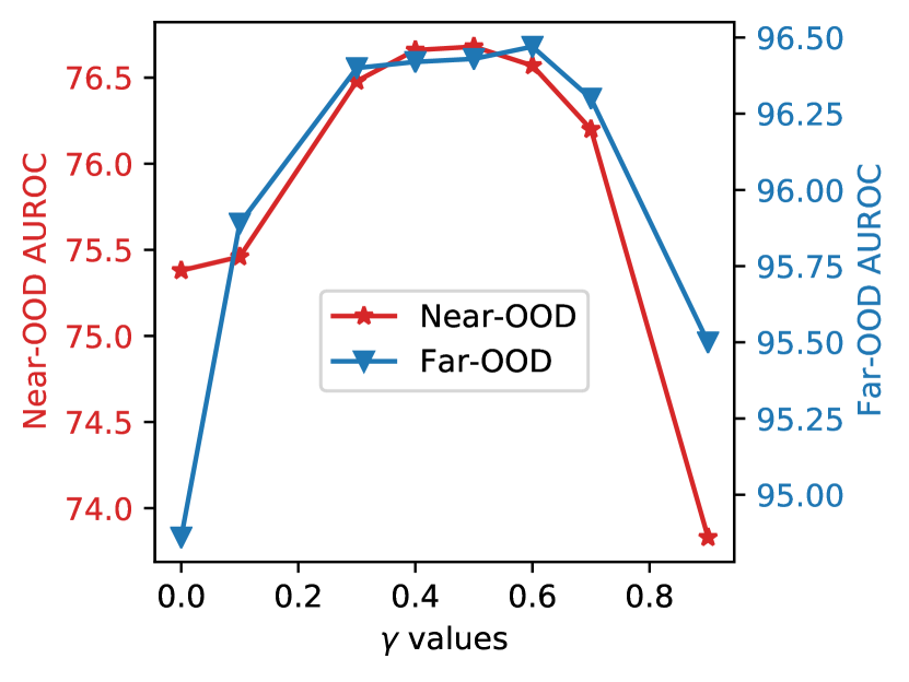
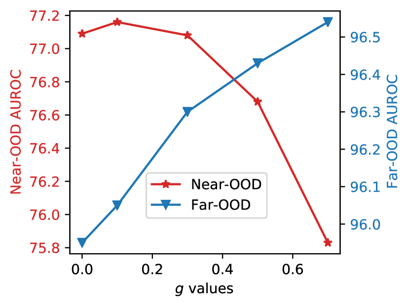
Threshold and gap in Eq. 3.2. As illustrated in Fig. 3, employing a moderate threshold (e.g., 0.4 < < 0.6) proves effective in distinguishing OOD samples across various scenarios. However, the efficacy of the gap parameter depends upon the specific characteristics of different OOD datasets. A larger facilitates the identification of more confidently classified ID/OOD samples, thereby improving the detection of far-OOD samples. Conversely, a smaller is advantageous for near-OOD detection as it accommodates low-confidence OOD samples, which are typically more prevalent in near-OOD scenarios.
In scenarios where the OOD distribution is entirely unknown, we adopt a conservative approach by setting to 0.5 in all experiments. This balanced setting provides a robust baseline for performance across a variety of conditions. However, if prior knowledge regarding the difficulty levels of OOD datasets is accessible, tailoring the hyperparameters—such as opting for a smaller in more challenging OOD contexts—can yield enhanced detection performance.
ID-OOD imbalanced Test Data. To investigate the stability of our method with imbalanced ID-OOD test data, we construct test sets with various mixture ratios of ID and OOD samples. Specifically, we adopted the 1.28M ImageNet training data as ID and randomly sampled 12.8K and 1.28K instances from the SUN OOD dataset to construct the ID:OOD ratios of 100:1 and 1000:1 settings, respectively. To construct the ID:OOD ratios of 1:100, 1:10, 1:1, and 10:1 settings, we randomly sampled 40K samples from the SUN dataset as OOD and randomly sampled 400, 4K, 40K, and 400K instances from the ImageNet training data. As shown in Tab. 5, our method outperforms NegLabel across a wide range of mixture ratios (from 1:100 to 100:1), validating the robustness and reliability of our approach. However, unbalanced mixture ratios do pose a challenge to our method. Our approach performs the best in scenarios with a balanced mixture of ID and OOD samples, reducing the FPR95 by 11.18%. As the mixture ratio becomes increasingly unbalanced, the improvement brought by our method gradually decreases. When the unbalanced ratio reaches 1000:1, our method shows some negative impact.
After a more detailed analysis, we discovered that the fundamental issue stems from the increased proportion of misclassified samples in the memory due to the growing ID-OOD imbalance. To effectively address this problem, we refine the selection criterion for memorizing OOD samples by adaptively adjusting the gap . We refer to this adaptive gap strategy as AdaGap, which significantly improves the robustness of our method against ID-OOD imbalanced test data, as demonstrated in Table 5. To summarize, we first estimate the ratio of ID to OOD in the test data online. If there is a higher proportion of ID/OOD compared to OOD/ID, we adjust the standards for caching ID/OOD data into memory by dynamically modifying the gap in Eq. 3.2. For more detailed implementation, please refer to the Appendix A.6.
| ID:OOD Ratio | 1:100 | 1:10 | 1:1 | 10:1 | 100:1 | 1K:1 |
|---|---|---|---|---|---|---|
| NegLabel | 22.42 | 21.11 | 20.99 | 20.92 | 21.48 | 23.69 |
| AdaNeg | 21.00 | 12.49 | 9.81 | 15.61 | 20.71 | 26.28 |
| AdaNeg (With AdaGap) | 20.50 | 12.22 | 9.73 | 12.98 | 15.61 | 18.43 |
| OOD datasets | ||||||
| Methods | CT-SCAN | X-Ray-Bone | Average | |||
| AUROC | FPR95 | AUROC | FPR95 | AUROC | FPR95 | |
| NegLabel | 63.53 | 100 | 99.68 | 0.56 | 81.61 | 50.28 |
| AdaNeg (Ours) | 93.48 | 100 | 99.99 | 0.11 | 96.74 | 50.06 |
Generalization to Other Domains. Besides experiments with natural images, we further validate our method on the BIMCV-COVID19+ dataset [61], which includes medical images, following the OpenOOD setup. Specifically, we select BIMCV as the ID dataset, which includes chest X-ray images CXR (CR, DX) of COVID-19 patients and healthy individuals. For the OOD datasets, we follow the OpenOOD setup and use CT-SCAN and X-Ray-Bone datasets. The CT-SCAN dataset includes computed tomography (CT) images of COVID-19 patients and healthy individuals, while the X-Ray-Bone dataset contains X-ray images of hands. As illustrated in Tab. 6, our AdaNeg method consistently outperforms NegLabel on this medical image dataset.
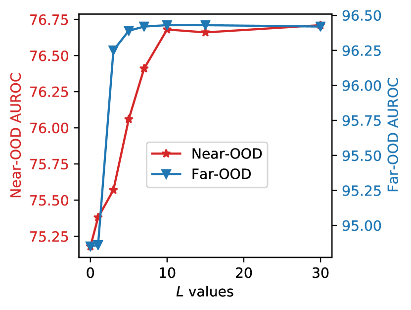
Memory Length. As demonstrated in Fig. 3(c), there is a positive correlation between the memory length and the performance outcomes, affirming the efficacy of feature memorization from another perspective. In all our experiments, we have set to 10.
Complexity Analyses. As analyzed in Table 4, our AdaNeg approach does not introduce any learnable parameters or require model training. Furthermore, it significantly enhances performance while maintaining a fast testing speed.
5 Conclusion and Limitations
We proposed adaptive negative proxies that aligned more effectively with OOD distributions, thereby providing more effective guidance for OOD detection. These proxies were constructed using a task-aware feature memory that selectively cached discriminative image features during testing. Our approach facilitated the generation of both task-adaptive and sample-adaptive proxies through carefully designed memory reading operations. Notably, our method was training-free and annotation-free, and it maintained fast testing speed and achieved state-of-the-art results on various benchmarks. These results validated the effectiveness of the proposed adaptive proxies.
One minor limitation of our method is the introduction of an external memory requirement. For example, this memory occupies a storage space of 214.75MB when using the ImageNet dataset as the ID, which may pose challenges for storage-constrained applications.
References
- [1] Yichen Bai, Zongbo Han, Changqing Zhang, Bing Cao, Xiaoheng Jiang, and Qinghua Hu. Id-like prompt learning for few-shot out-of-distribution detection. arXiv preprint arXiv:2311.15243, 2023.
- [2] Julian Bitterwolf, Maximilian Mueller, and Matthias Hein. In or out? fixing imagenet out-of-distribution detection evaluation. In ICML, 2023.
- [3] Chaoqi Chen, Jiongcheng Li, Hong-Yu Zhou, Xiaoguang Han, Yue Huang, Xinghao Ding, and Yizhou Yu. Relation matters: Foreground-aware graph-based relational reasoning for domain adaptive object detection. IEEE Transactions on Pattern Analysis and Machine Intelligence, 45(3):3677–3694, 2022.
- [4] Chaoqi Chen, Luyao Tang, Yue Huang, Xiaoguang Han, and Yizhou Yu. Coda: generalizing to open and unseen domains with compaction and disambiguation. Advances in Neural Information Processing Systems, 36, 2023.
- [5] Chaoqi Chen, Luyao Tang, Leitian Tao, Hong-Yu Zhou, Yue Huang, Xiaoguang Han, and Yizhou Yu. Activate and reject: towards safe domain generalization under category shift. In Proceedings of the IEEE/CVF International Conference on Computer Vision, pages 11552–11563, 2023.
- [6] Yihong Chen, Yue Cao, Han Hu, and Liwei Wang. Memory enhanced global-local aggregation for video object detection. In Proceedings of the IEEE/CVF conference on computer vision and pattern recognition, pages 10337–10346, 2020.
- [7] Mircea Cimpoi, Subhransu Maji, Iasonas Kokkinos, Sammy Mohamed, and Andrea Vedaldi. Describing textures in the wild. In Proceedings of the IEEE conference on computer vision and pattern recognition, pages 3606–3613, 2014.
- [8] Hanming Deng, Yang Hua, Tao Song, Zongpu Zhang, Zhengui Xue, Ruhui Ma, Neil Robertson, and Haibing Guan. Object guided external memory network for video object detection. In Proceedings of the IEEE/CVF International Conference on Computer Vision, pages 6678–6687, 2019.
- [9] Jia Deng, Wei Dong, Richard Socher, Li-Jia Li, Kai Li, and Li Fei-Fei. Imagenet: A large-scale hierarchical image database. In 2009 IEEE conference on computer vision and pattern recognition, pages 248–255. Ieee, 2009.
- [10] Li Deng. The mnist database of handwritten digit images for machine learning research [best of the web]. IEEE signal processing magazine, 29(6):141–142, 2012.
- [11] Andrija Djurisic, Nebojsa Bozanic, Arjun Ashok, and Rosanne Liu. Extremely simple activation shaping for out-of-distribution detection. arXiv preprint arXiv:2209.09858, 2022.
- [12] Xuefeng Du, Gabriel Gozum, Yifei Ming, and Yixuan Li. Siren: Shaping representations for detecting out-of-distribution objects. Advances in Neural Information Processing Systems, 35:20434–20449, 2022.
- [13] Xuefeng Du, Xin Wang, Gabriel Gozum, and Yixuan Li. Unknown-aware object detection: Learning what you don’t know from videos in the wild. In Proceedings of the IEEE/CVF Conference on Computer Vision and Pattern Recognition, pages 13678–13688, 2022.
- [14] Xuefeng Du, Zhaoning Wang, Mu Cai, and Yixuan Li. Vos: Learning what you don’t know by virtual outlier synthesis. arXiv preprint arXiv:2202.01197, 2022.
- [15] Sepideh Esmaeilpour, Bing Liu, Eric Robertson, and Lei Shu. Zero-shot out-of-distribution detection based on the pre-trained model clip. In Proceedings of the AAAI conference on artificial intelligence, volume 36, pages 6568–6576, 2022.
- [16] Ke Fan, Yikai Wang, Qian Yu, Da Li, and Yanwei Fu. A simple test-time method for out-of-distribution detection. arXiv preprint arXiv:2207.08210, 2022.
- [17] Stanislav Fort, Jie Ren, and Balaji Lakshminarayanan. Exploring the limits of out-of-distribution detection. Advances in Neural Information Processing Systems, 34:7068–7081, 2021.
- [18] Zhitong Gao, Shipeng Yan, and Xuming He. Atta: Anomaly-aware test-time adaptation for out-of-distribution detection in segmentation. Advances in Neural Information Processing Systems, 36:45150–45171, 2023.
- [19] Kaiming He, Xiangyu Zhang, Shaoqing Ren, and Jian Sun. Deep residual learning for image recognition. In Proceedings of the IEEE conference on computer vision and pattern recognition, pages 770–778, 2016.
- [20] Dan Hendrycks and Kevin Gimpel. A baseline for detecting misclassified and out-of-distribution examples in neural networks. arXiv preprint arXiv:1610.02136, 2016.
- [21] Dan Hendrycks, Mantas Mazeika, and Thomas Dietterich. Deep anomaly detection with outlier exposure. arXiv preprint arXiv:1812.04606, 2018.
- [22] Dan Hendrycks, Mantas Mazeika, Saurav Kadavath, and Dawn Song. Using self-supervised learning can improve model robustness and uncertainty. Advances in neural information processing systems, 32, 2019.
- [23] Dan Hendrycks, Norman Mu, Ekin D Cubuk, Barret Zoph, Justin Gilmer, and Balaji Lakshminarayanan. Augmix: A simple data processing method to improve robustness and uncertainty. arXiv preprint arXiv:1912.02781, 2019.
- [24] Dan Hendrycks, Andy Zou, Mantas Mazeika, Leonard Tang, Bo Li, Dawn Song, and Jacob Steinhardt. Pixmix: Dreamlike pictures comprehensively improve safety measures. In Proceedings of the IEEE/CVF Conference on Computer Vision and Pattern Recognition, pages 16783–16792, 2022.
- [25] Rui Huang, Andrew Geng, and Yixuan Li. On the importance of gradients for detecting distributional shifts in the wild. Advances in Neural Information Processing Systems, 34:677–689, 2021.
- [26] Rui Huang and Yixuan Li. Mos: Towards scaling out-of-distribution detection for large semantic space. In Proceedings of the IEEE/CVF Conference on Computer Vision and Pattern Recognition, pages 8710–8719, 2021.
- [27] Xue Jiang, Feng Liu, Zhen Fang, Hong Chen, Tongliang Liu, Feng Zheng, and Bo Han. Negative label guided OOD detection with pretrained vision-language models. In The Twelfth International Conference on Learning Representations, 2024.
- [28] Geethan Karunaratne, Manuel Schmuck, Manuel Le Gallo, Giovanni Cherubini, Luca Benini, Abu Sebastian, and Abbas Rahimi. Robust high-dimensional memory-augmented neural networks. Nature communications, 12(1):2468, 2021.
- [29] Shu Kong and Deva Ramanan. Opengan: Open-set recognition via open data generation. In Proceedings of the IEEE/CVF International Conference on Computer Vision, pages 813–822, 2021.
- [30] Alex Krizhevsky, Geoffrey Hinton, et al. Learning multiple layers of features from tiny images. 2009.
- [31] Alex Krizhevsky, Ilya Sutskever, and Geoffrey E Hinton. Imagenet classification with deep convolutional neural networks. Advances in neural information processing systems, 25, 2012.
- [32] Ya Le and Xuan Yang. Tiny imagenet visual recognition challenge. CS 231N, 7(7):3, 2015.
- [33] Kimin Lee, Kibok Lee, Honglak Lee, and Jinwoo Shin. A simple unified framework for detecting out-of-distribution samples and adversarial attacks. Advances in neural information processing systems, 31, 2018.
- [34] Tianqi Li, Guansong Pang, Xiao Bai, Wenjun Miao, and Jin Zheng. Learning transferable negative prompts for out-of-distribution detection. In Proceedings of the IEEE/CVF Conference on Computer Vision and Pattern Recognition, pages 17584–17594, 2024.
- [35] Jian Liang, Ran He, and Tieniu Tan. A comprehensive survey on test-time adaptation under distribution shifts. arXiv preprint arXiv:2303.15361, 2023.
- [36] Shiyu Liang, Yixuan Li, and Rayadurgam Srikant. Enhancing the reliability of out-of-distribution image detection in neural networks. arXiv preprint arXiv:1706.02690, 2017.
- [37] Weitang Liu, Xiaoyun Wang, John Owens, and Yixuan Li. Energy-based out-of-distribution detection. Advances in neural information processing systems, 33:21464–21475, 2020.
- [38] Xixi Liu, Yaroslava Lochman, and Christopher Zach. Gen: Pushing the limits of softmax-based out-of-distribution detection. In Proceedings of the IEEE/CVF Conference on Computer Vision and Pattern Recognition, pages 23946–23955, 2023.
- [39] Yifei Ming, Ziyang Cai, Jiuxiang Gu, Yiyou Sun, Wei Li, and Yixuan Li. Delving into out-of-distribution detection with vision-language representations. Advances in Neural Information Processing Systems, 35:35087–35102, 2022.
- [40] Yifei Ming and Yixuan Li. How does fine-tuning impact out-of-distribution detection for vision-language models? International Journal of Computer Vision, 132(2):596–609, 2024.
- [41] Yifei Ming, Yiyou Sun, Ousmane Dia, and Yixuan Li. How to exploit hyperspherical embeddings for out-of-distribution detection? arXiv preprint arXiv:2203.04450, 2022.
- [42] Atsuyuki Miyai, Qing Yu, Go Irie, and Kiyoharu Aizawa. Locoop: Few-shot out-of-distribution detection via prompt learning. Advances in Neural Information Processing Systems, 36, 2024.
- [43] Yuval Netzer, Tao Wang, Adam Coates, Alessandro Bissacco, Baolin Wu, Andrew Y Ng, et al. Reading digits in natural images with unsupervised feature learning. In NIPS workshop on deep learning and unsupervised feature learning, volume 2011, page 7. Granada, Spain, 2011.
- [44] Anh Nguyen, Jason Yosinski, and Jeff Clune. Deep neural networks are easily fooled: High confidence predictions for unrecognizable images. In Proceedings of the IEEE conference on computer vision and pattern recognition, pages 427–436, 2015.
- [45] Jun Nie, Yonggang Zhang, Zhen Fang, Tongliang Liu, Bo Han, and Xinmei Tian. Out-of-distribution detection with negative prompts. In The Twelfth International Conference on Learning Representations, 2024.
- [46] Seoung Wug Oh, Joon-Young Lee, Ning Xu, and Seon Joo Kim. Video object segmentation using space-time memory networks. In Proceedings of the IEEE/CVF International Conference on Computer Vision, pages 9226–9235, 2019.
- [47] Charles Packer, Vivian Fang, Shishir G Patil, Kevin Lin, Sarah Wooders, and Joseph E Gonzalez. Memgpt: Towards llms as operating systems. arXiv preprint arXiv:2310.08560, 2023.
- [48] Alec Radford, Jong Wook Kim, Chris Hallacy, Aditya Ramesh, Gabriel Goh, Sandhini Agarwal, Girish Sastry, Amanda Askell, Pamela Mishkin, Jack Clark, et al. Learning transferable visual models from natural language supervision. In International conference on machine learning, pages 8748–8763. PMLR, 2021.
- [49] Jie Ren, Stanislav Fort, Jeremiah Liu, Abhijit Guha Roy, Shreyas Padhy, and Balaji Lakshminarayanan. A simple fix to mahalanobis distance for improving near-ood detection. arXiv preprint arXiv:2106.09022, 2021.
- [50] Seonghan Ryu, Sangjun Koo, Hwanjo Yu, and Gary Geunbae Lee. Out-of-domain detection based on generative adversarial network. In Proceedings of the 2018 Conference on Empirical Methods in Natural Language Processing, pages 714–718, 2018.
- [51] Adam Santoro, Sergey Bartunov, Matthew Botvinick, Daan Wierstra, and Timothy Lillicrap. Meta-learning with memory-augmented neural networks. In International conference on machine learning, pages 1842–1850. PMLR, 2016.
- [52] Walter J Scheirer, Anderson de Rezende Rocha, Archana Sapkota, and Terrance E Boult. Toward open set recognition. IEEE transactions on pattern analysis and machine intelligence, 35(7):1757–1772, 2012.
- [53] Vikash Sehwag, Mung Chiang, and Prateek Mittal. Ssd: A unified framework for self-supervised outlier detection. arXiv preprint arXiv:2103.12051, 2021.
- [54] Manli Shu, Weili Nie, De-An Huang, Zhiding Yu, Tom Goldstein, Anima Anandkumar, and Chaowei Xiao. Test-time prompt tuning for zero-shot generalization in vision-language models. Advances in Neural Information Processing Systems, 35:14274–14289, 2022.
- [55] Sainbayar Sukhbaatar, Jason Weston, Rob Fergus, et al. End-to-end memory networks. Advances in neural information processing systems, 28, 2015.
- [56] Yiyou Sun, Chuan Guo, and Yixuan Li. React: Out-of-distribution detection with rectified activations. Advances in Neural Information Processing Systems, 34:144–157, 2021.
- [57] Yiyou Sun, Yifei Ming, Xiaojin Zhu, and Yixuan Li. Out-of-distribution detection with deep nearest neighbors. In International Conference on Machine Learning, pages 20827–20840. PMLR, 2022.
- [58] Jihoon Tack, Sangwoo Mo, Jongheon Jeong, and Jinwoo Shin. Csi: Novelty detection via contrastive learning on distributionally shifted instances. Advances in neural information processing systems, 33:11839–11852, 2020.
- [59] Leitian Tao, Xuefeng Du, Xiaojin Zhu, and Yixuan Li. Non-parametric outlier synthesis. arXiv preprint arXiv:2303.02966, 2023.
- [60] Grant Van Horn, Oisin Mac Aodha, Yang Song, Yin Cui, Chen Sun, Alex Shepard, Hartwig Adam, Pietro Perona, and Serge Belongie. The inaturalist species classification and detection dataset. In Proceedings of the IEEE conference on computer vision and pattern recognition, pages 8769–8778, 2018.
- [61] Maria De La Iglesia Vayá, Jose Manuel Saborit, Joaquim Angel Montell, Antonio Pertusa, Aurelia Bustos, Miguel Cazorla, Joaquin Galant, Xavier Barber, Domingo Orozco-Beltrán, Francisco García-García, et al. Bimcv covid-19+: a large annotated dataset of rx and ct images from covid-19 patients. arXiv preprint arXiv:2006.01174, 2020.
- [62] Sagar Vaze, Kai Han, Andrea Vedaldi, and Andrew Zisserman. Open-set recognition: A good closed-set classifier is all you need? arXiv preprint arXiv:2110.06207, 2021.
- [63] Dequan Wang, Evan Shelhamer, Shaoteng Liu, Bruno Olshausen, and Trevor Darrell. Tent: Fully test-time adaptation by entropy minimization. arXiv preprint arXiv:2006.10726, 2020.
- [64] Haoqi Wang, Zhizhong Li, Litong Feng, and Wayne Zhang. Vim: Out-of-distribution with virtual-logit matching. In Proceedings of the IEEE/CVF conference on computer vision and pattern recognition, pages 4921–4930, 2022.
- [65] Hualiang Wang, Yi Li, Huifeng Yao, and Xiaomeng Li. Clipn for zero-shot ood detection: Teaching clip to say no. In Proceedings of the IEEE/CVF International Conference on Computer Vision, pages 1802–1812, 2023.
- [66] Yezhen Wang, Bo Li, Tong Che, Kaiyang Zhou, Ziwei Liu, and Dongsheng Li. Energy-based open-world uncertainty modeling for confidence calibration. In Proceedings of the IEEE/CVF International Conference on Computer Vision, pages 9302–9311, 2021.
- [67] Jason Weston, Sumit Chopra, and Antoine Bordes. Memory networks. arXiv preprint arXiv:1410.3916, 2014.
- [68] Jianxiong Xiao, James Hays, Krista A Ehinger, Aude Oliva, and Antonio Torralba. Sun database: Large-scale scene recognition from abbey to zoo. In 2010 IEEE computer society conference on computer vision and pattern recognition, pages 3485–3492. IEEE, 2010.
- [69] Guo-Sen Xie, Huan Xiong, Jie Liu, Yazhou Yao, and Ling Shao. Few-shot semantic segmentation with cyclic memory network. In Proceedings of the IEEE/CVF International Conference on Computer Vision, pages 7293–7302, 2021.
- [70] Kai Xu, Rongyu Chen, Gianni Franchi, and Angela Yao. Scaling for training time and post-hoc out-of-distribution detection enhancement. arXiv preprint arXiv:2310.00227, 2023.
- [71] Jingkang Yang, Pengyun Wang, Dejian Zou, Zitang Zhou, Kunyuan Ding, Wenxuan Peng, Haoqi Wang, Guangyao Chen, Bo Li, Yiyou Sun, Xuefeng Du, Kaiyang Zhou, Wayne Zhang, Dan Hendrycks, Yixuan Li, and Ziwei Liu. Openood: Benchmarking generalized out-of-distribution detection. 2022.
- [72] Puning Yang, Jian Liang, Jie Cao, and Ran He. Auto: Adaptive outlier optimization for online test-time ood detection. arXiv preprint arXiv:2303.12267, 2023.
- [73] Jingyang Zhang, Nathan Inkawhich, Yiran Chen, and Hai Li. Fine-grained out-of-distribution detection with mixup outlier exposure. CoRR, (abs/2106.03917), 2021.
- [74] Jingyang Zhang, Jingkang Yang, Pengyun Wang, Haoqi Wang, Yueqian Lin, Haoran Zhang, Yiyou Sun, Xuefeng Du, Kaiyang Zhou, Wayne Zhang, Yixuan Li, Ziwei Liu, Yiran Chen, and Hai Li. Openood v1.5: Enhanced benchmark for out-of-distribution detection. arXiv preprint arXiv:2306.09301, 2023.
- [75] Yabin Zhang, Bin Deng, Hui Tang, Lei Zhang, and Kui Jia. Unsupervised multi-class domain adaptation: Theory, algorithms, and practice. IEEE Transactions on Pattern Analysis and Machine Intelligence, 44(5):2775–2792, 2020.
- [76] Yabin Zhang, Wenjie Zhu, Chenhang He, and Lei Zhang. Lapt: Label-driven automated prompt tuning for ood detection with vision-language models. 2024.
- [77] Yabin Zhang, Wenjie Zhu, Hui Tang, Zhiyuan Ma, Kaiyang Zhou, and Lei Zhang. Dual memory networks: A versatile adaptation approach for vision-language models. In Proceedings of the IEEE/CVF conference on computer vision and pattern recognition, pages 28718–28728, 2024.
- [78] Bolei Zhou, Agata Lapedriza, Aditya Khosla, Aude Oliva, and Antonio Torralba. Places: A 10 million image database for scene recognition. IEEE transactions on pattern analysis and machine intelligence, 40(6):1452–1464, 2017.
Appendix A Appendix
A.1 ID-Similarity to OOD Ratio with ground truth ID and OOD labels
We introduce the ID-Similarity to OOD Ratio (ISOR) to quantitatively measure the relative alignment of negative proxies with ground truth OOD labels, compared to their alignment with ID labels. In implementation, we adapt the score function of NegLabel (i.e., Eq. 4), which originally measures the similarity of a test image to ID labels over negative labels. We modify this function by replacing the negative labels with ground truth OOD labels and changing the input from test images to negative proxies (e.g., negative texts), while keeping other aspects consistent with Eq. 4. This modified score function allows us to assess the degree of similarity between the inputs and ground truth ID/OOD labels, thereby quantifying the relative alignment between negative proxies and OOD labels. Specifically, lower ISOR indicates a higher similarity to OOD labels and a reduced similarity to ID labels.
A.2 Entropy-based caching strategy for full memory
The memory we construct is of finite length; hence, as the number of cached images increases, it may become fully occupied. To address this, we have devised a simple strategy to retain only those images with low entropy, e.g., high confidence. Specifically, when storing an image in memory, we also record its entropy pertinent to OOD detection:
| (A.1) |
where represents the probability of belonging to the ID, as shown in Eq. (4). Given the entropy of the current test image and a full memory , we replace the item with the maximum entropy in with the current image feature if the current test image exhibits lower entropy. Otherwise, we do not cache the current test sample.
A.3 Evaluation criteria
Following common practice [26, 39, 27], we employ the following three evaluation metrics: (1) FPR95, which measures the false positive rate for OOD samples when the detection accuracy for ID samples is at 95%; (2) AUROC, the area under the receiver operating characteristic curve; and (3) ID ACC, which quantifies the accuracy of correctly identifying and classifying ID samples.
A.4 Detailed results on ImageNet dataset under OpenOOD setting
The detailed OOD detection results on the OpenOOD benchmark are presented in Tab. A7.
A.5 Results on CIFAR10/100
As illustrated in Tab. A8, the advantage of our AdaNeg also holds on the CIFAR10/100 dataset. Notably, our method achieves new state-of-the-art results in the far-OOD setting under a zero-shot training-free manner, even outperforming its competitors training on the full labeled training set.
| Near-/Far-OOD | Datasets | FPR95 | AUROC |
|---|---|---|---|
| Near-OOD | SSB-hard [62] | 74.91 | 75.11 |
| NINCO [2] | 60.10 | 78.30 | |
| Mean | 67.51 | 76.70 | |
| Far-OOD | iNaturalist [60] | 0.72 | 99.72 |
| Textures [7] | 21.40 | 95.71 | |
| OpenImage-O [64] | 29.81 | 93.87 | |
| Mean | 17.31 | 96.43 |
| Methods | FPR95 | |||
|---|---|---|---|---|
| Near-OOD | Far-OOD | Near-OOD | Far-OOD | |
| Methods requiring training (or fine-tuning) | ||||
| PixMix [24] + KNN [57] | – | – | 93.10 | 95.94 |
| OE [21] + MSP [20] | – | – | 94.82 | 96.00 |
| PixMix [24] + RotPred [22] | – | – | 94.86 | 98.18 |
| Zero-shot Training-free Methods | ||||
| MCM [39] | 30.86 | 17.99 | 91.92 | 95.54 |
| NegLabel [27] | 28.75 | 6.60 | 94.58 | 98.39 |
| AdaNeg (Ours) | 20.40 | 2.79 | 94.78 | 99.26 |
| Methods | FPR95 | |||
|---|---|---|---|---|
| Near-OOD | Far-OOD | Near-OOD | Far-OOD | |
| Methods requiring training (or fine-tuning) | ||||
| GEN [38] | – | – | 81.31 | 79.68 |
| VOS [14] + EBO [37] | – | – | 80.93 | 81.32 |
| SCALE [70] | – | – | 80.99 | 81.42 |
| OE [21] + MSP [20] | – | – | 88.30 | 81.41 |
| Zero-shot Training-free Methods | ||||
| MCM [39] | 75.20 | 59.32 | 71.00 | 76.00 |
| NegLabel [27] | 71.44 | 40.92 | 70.58 | 89.68 |
| AdaNeg (Ours) | 59.07 | 29.35 | 84.62 | 95.25 |
| Near-/Far-OOD | Datasets | FPR95 | AUROC |
|---|---|---|---|
| Near-OOD | CIFAR10 [30] | 58.24 | 79.91 |
| TIN [32] | 59.90 | 89.34 | |
| Mean | 59.07 | 84.62 | |
| Far-OOD | MNIST [10] | 4.18 | 97.90 |
| SVHN [43] | 6.03 | 97.60 | |
| Texture [7] | 30.00 | 95.14 | |
| Places365 [78] | 77.20 | 90.35 | |
| Mean | 29.35 | 95.25 |
| Near-/Far-OOD | Datasets | FPR95 | AUROC |
|---|---|---|---|
| Near-OOD | CIFAR100 [30] | 35.80 | 90.93 |
| TIN [32] | 5.01 | 98.63 | |
| Mean | 20.40 | 94.78 | |
| Far-OOD | MNIST [10] | 0.13 | 99.96 |
| SVHN [43] | 0.04 | 99.97 | |
| Texture [7] | 0.04 | 99.82 | |
| Places365 [78] | 10.93 | 97.29 | |
| Mean | 2.79 | 99.26 |
A.6 More analyses
Detailed Implementation of AdaGap Module. We have implemented an adaptive gap (AdaGap) module to adjust the memorization selection criteria dynamically. This strategy builds on the observation that as the score increases/decreases, the probability that a sample is ID/OOD also increases accordingly. By enforcing a stringent selection criterion, we can effectively minimize the inclusion of misclassified samples in our memory. Specifically, we first online estimate the ratio of ID to OOD samples in the test data using a First-In-First-Out queue, which caches the ID/OOD estimation (cf. Eq. 3.2) of the most recent samples:
| (A.2) |
where the ID and OOD numbers are acquired within the queue.
Leveraging the estimated mix ratio (), we can dynamically adjust the gap in memory caching to avoid a majority of misclassified samples within the memory. For instance, if we find that ID samples constitute the majority of the test samples (i.e., > 0.5), this could lead to an increased proportion of ID samples in the OOD memory. In response, we can adjust the selection criterion for OOD memorization to only cache higher confidence OOD samples. This adjustment is achieved by modifying the selection criterion for memorization in Eq. 3.2 as follows:
| (A.3) |
where is the default gap analyzed in Figure 3(b). In this way, under ID/OOD balanced conditions (i.e., = 0.5), our method aligns with our original version. However, if the proportion of ID samples is higher in the test samples’ estimation (i.e., > 0.5), we raise the standard for storing negative samples in the memory. In an extreme case when = 1, we estimate that there might be no OOD samples among the test samples; thus, we stop storing test samples in the negative memory and only selectively cache test samples into the positive memory. We adjust our approach conversely when the value is lower than 0.5.
Please note that the selection criterion is dynamically adjusted online because the is estimated with the most recent test samples. Here, we set by default. This dynamic adjustment ensures that our memory caching strategy remains responsive to the evolving nature of the test sample distribution, thereby optimizing memory utilization and enhancing the accuracy of our domain distinction process.
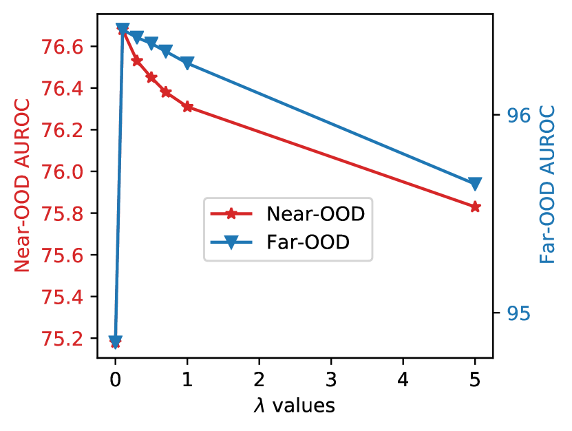
in Eq. 13. As illustrated in Fig. 4(a), the OOD detection performance remains robust across a wide range of values, e.g., from 0.01 to 1. For all experiments, we have set to 0.1.
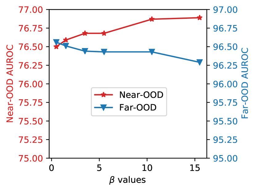
in Eq. 11. Results with different values are shown in Fig. 4(b), where OOD detection performance is robust to the values. We adopt =5.5 in all experiments.
Ordering of Testing Data. Our AdaNeg selectively caches test data into memory, potentially causing variations in the results depending on the ordering of the test data. To rigorously test this aspect, we randomly shuffled the order of the test data using three distinct seeds. We observed that our method exhibits robustness to changes in the ordering of test data. Specifically, across three experiments conducted on the ImageNet dataset, the AUROC scores were 96.65%, 96.69%, and 96.64%, respectively, demonstrating fluctuations of less than 0.1%. We report the average results from three random runs in our paper.
Various Backbone Architectures. Results with various VLMs architectures are illustrated in Tab. A11, where better results are typically achieved with stronger backbones.
| OOD datasets | ||||||||||
|---|---|---|---|---|---|---|---|---|---|---|
| Backbone | INaturalist | Sun | Places | Textures | Average | |||||
| AUROC | FPR95 | AUROC | FPR95 | AUROC | FPR95 | AUROC | FPR95 | AUROC | FPR95 | |
| ResNet50 | 99.58 | 1.18 | 97.37 | 10.56 | 93.84 | 43.19 | 94.18 | 35.00 | 96.24 | 22.48 |
| VITL/32 | 99.59 | 1.02 | 97.53 | 9.63 | 93.99 | 38.45 | 94.21 | 37.92 | 96.33 | 21.76 |
| VITB/16 | 99.71 | 0.59 | 97.44 | 9.50 | 94.55 | 34.34 | 94.93 | 31.27 | 96.66 | 18.92 |
Complementarity to Training-based Method. We validated the complementarity between our AdaNeg method and the latest works, NegPrompt [34] and LAPT [76], which use learned prompts. As shown in Table A12, our method significantly improves performance over these approaches, demonstrating its complementarity with training-based methods.
| Methods | INaturalist | SUN | Places | Textures | Average |
|---|---|---|---|---|---|
| NegPrompt [34] | 6.76 | 23.41 | 28.32 | 34.57 | 23.27 |
| + AdaNeg | 3.87 | 11.35 | 25.45 | 29.79 | 17.62 |
| LAPT [76] | 1.10 | 20.59 | 35.38 | 40.11 | 24.29 |
| + AdaNeg | 0.58 | 9.98 | 30.47 | 24.25 | 16.32 |
Number of Testing Data. We examine the dependency of our approach on the number of test images by evaluating its performance across different scales of test samples. As the number of test samples increases (from 900 to 90K), the cached feature data also increases, leading to an improvement in our method’s results, as shown in Tab. A13. Even with a small number of test samples (e.g., 90 and 900), our method significantly reduces FPR95 compared to NegLabel, demonstrating its robustness across different numbers of test images.
Note that with only 90 test images, the task of distinguishing between ID and OOD samples degenerates into a simpler task since the number of test images is even smaller than the number of classes (e.g., 1000 for ImageNet). Consequently, both NegLabel and our method achieve lower FPR95 in such an easier scenario.
| Num. of Test Images | 90 | 900 | 9K | 45K | 90K |
|---|---|---|---|---|---|
| NegLabel | 14.00 | 20.44 | 20.71 | 20.51 | 20.53 |
| AdaNeg | 6.00 | 10.12 | 9.78 | 9.66 | 9.50 |