Peculiarities of hydraulic fracture propagation in media with heterogeneous toughness: the energy balance, elastic battery and fluid backflow

Abstract

This paper investigates hydraulic fracture in a media with periodic heterogeneous toughness. Results for the plane-strain (KGD) model are analysed. The energy distribution as the fracture propagates is examined, along with the evolution of the crack geometry. It is shown that the solid layer acts as an elastic battery, discharging to promote rapid propagation through weaker material layers. The limiting behaviour as length $L\to\infty$ is discussed. The velocity of the fluid throughout the crack length is also considered. For fractures in high-toughness material it is shown that fluid backflow can occur, with its profile dependent on the toughness distribution. The implications of these findings are discussed.

1 Introduction

Hydraulic fracture (HF) is the process of a fluid-drive crack propagating in a solid material. This process occurs in many forms, both in nature and industrial applications, such as: fracking shale to obtain natural gas, deposition of CO₂ rich fluid during carbon storage, the evolution of volcanic dykes, and subglacial drainage. Consequently, hydraulic fracture modelling and the study of HF-related effects have been an active field of research for decades. Amongst the earliest approaches are the 1D models, including the Kristianovich-Geertsma-de Klerk (KGD, plane strain) approximation [Khristianovic Zheltov, 1955, Geertsma and de Klerk, 1969]. Although since superseded in most applications, the fact that it is more easily modified than later models makes it useful for incorporating and testing previously unincorporated effects, and analysing their impact on the HF process.

One such important effect is the impact of heterogeneity of the fracture media, which has typically been neglected in HF models due to the complexity of the problem. In particular, while homogenisation strategies exist for the Young’s modulus and other parameters, homogenisation of the fracture toughness $K_{Ic}$ cannot generally be done in a straightforward way (see e.g.  [Kachanov and Sevostianov, 2018, Ponson, 2023]). Therefore, if heterogeneous toughness is to be incorporated via homogenisation, further investigation is needed to develop effective strategies. Heterogeneity of the toughness can also lead to secondary consequences of importance, such as crack deflection [Zeng and Wei, 2017], and the impact on transport of dissolved CO₂ within fractures related to carbon-storage (and therefore the potential for CO₂ leak-off) [Chen et al., 2024].

Concerning homogenization of the fracture toughness in the context of HF, a general discussion was given in the introductions of [Da Fies et al., 2022, Oyedokun and Schubert, 2017]. There is also the recent work of [Sarmadi et al., 2024], who proposed an approach to dealing with fracture in heterogeneous media where there was no clear distinction between rock layers utilizing a stochastic-based method, as well as the work of [Da Fies et al., 2021, Da Fies et al., 2022, Da Fies et al., 2023] where a temporal-averaging based approach was proposed, claiming that it provided the optimal ‘average’ toughness.

Testing these homogenisation strategies, and the perculiarities of HF propagating in heterogeneous media, requires numerical simulations. FEM techniques (see for example [Li et al., 2020] and references therein) constitute an effective approach; we mention, in particular, the mesh-transition technique for use within an ABAQUS environment by [Rueda et al., 2023], the phase-field approach for porous media was developed by [Sarmadi et al., 2024], and the sandwich-layered structure model of multi-layered rockbeds by [Zhong et al., 2024].

An alternative method for modelling HF propagating in media with heterogeneous toughness is based on the ‘universal algorithm’ approach. This was developed by [Wrobel and Mishuris, 2015] in the context of the 1D fracture models (PKN, KGD, radial), before later being extended to the case of heterogeneous media as outlined in [Da Fies, 2020]. We can mention methods of modelling more general planar fractures in layered rocks, such as an approach using the 3D-displacement discontinuity method by [Li et al., 2024]. An alternative approach, based on incorporating conditions for initiation of crack propagation between distinct rock layers [Peruzzo et al., 2021, Peruzzo and Lecampion, 2024] within the level-set method was given by [Peruzzo, 2023]. This has been applied to analyses of the effect of rock heterogeneity on crack arrest in the case of buoyant fractures [Möri et al., 2024]. It should be noted that [Wang et al., 2024] suggested the system asymptotics, which are utilized by these approaches when obtaining solutions need to be updated, since the solutions may lose accuracy in cases of cracks propagating between material layers. They have suggested that an additional ’intermediate’ asymptotic solution needs to be utilized, in addition to the crack-tip and far-field asymptotics.

Experimental investigations have also been conducted. For example, HF propagating along weak interfaces was examined by [Stanchits et al., 2015], where the fracture path was found to be neither symmetrical nor planar. Other experimental results for materials with heterogeneous toughness [Shi et al., 2023] confirmed that the present of heterogeneities promotes more tortuous fracture paths. Also, a difference between near-wellbore and far-field behaviour was observed, particularly regarding fracture arrest and diversion (around inhomogeneities), hypothesising that they were related to the elastic energy available over the fracture length.

Figure 1: The KGD fracture propagating periodic toughness layers.

We note that analyses of the fracture energy can be completed utilizing existing formulations for the energy balance during HF propagation. This was derived for a planar hydraulic fracture with fluid lag by [Lecampion and Detournay, 2007], and extended to the case of multiple hydraulic fractures by [Bunger, 2013]. Very recently, an investigation of the energy balance in a hydraulic fracture at depth was provided in [Peruzzo et al., 2024]. However, these works assumed homogeneous fracture toughness; the effect of its heterogeneity has yet to be examined.

The present work carries out this investigation of the energy balance for HF in heterogeneous media, while also extending the results from [Da Fies et al., 2022]. That paper focused on strategies for evaluating the average toughness, and as such neglected discussion of processes not involved in the averaging procedure. Here, we provide an overview of peculiar features of hydraulic fracture propagation in heterogeneous materials, concentrating on those that are extremely relevant for HF modelling. Results obtained for the KGD model using the ‘universal-solver’ algorithm [Da Fies, 2020] are analysed, with particular focus on the crack geometry, energy balance, crack/ fluid velocities, and the limiting behaviour of the propagation regime.

The paper is organised as follows. The problem formulation is introduced in Sect. 2. This includes the governing equations, distribution of the periodic toughness heterogeneity, and approaches to characterising the fracture regime local to the crack tip. Limiting behaviour of this regime parameter are investigated. In Sect. 3, the energy distribution during fracture of heterogeneous media is considered in detail. In Sect. 4 the velocity of the crack tip is investigated, followed by an examination of the fluid behaviour within the fracture. Concluding remarks are given in Sect. 5. Some of the limiting analysis and figures are relegated to the Appendices for the sake of readability.

2 The KGD problem with a periodic fracture toughness distribution

2.1 Problem formulation with periodic toughness

The Kristianovich-Geertsma-de Klerk (KGD, plane strain) model [Khristianovic Zheltov, 1955, Geertsma and de Klerk, 1969] assumes of crack situated in the plane $x\in[-l(t),l(t)]$, that is symmetrical about the midpoint $x=0$ such that only the length $x\geq 0$ needs to be considered. The crack has fixed height $H$, while it’s length $2l(t)$ and aperture $w(t,x)$ change in time as the fracture advances (see Fig. 1). The crack growth is driven by a Newtonian fluid that is injected at the point $x=0$ at a known rate $Q_{0}(t)$. A periodic toughness distribution is assumed, with spacial period $X$, the material toughness at the crack tip being a function of the crack length $K_{Ic}(l(t))$. We normalise the crack length as $L(t)=l(t)/X$, so that each toughness period is of length $1$. Further details on the toughness distribution are provided in Sect. 2.1.1. Fluid leak-off into the surrounding domain, alongside any fluid-lag at the crack tip, are neglected.

2.1.1 Distribution of the material toughness

The material toughness distribution is assumed to vary between two values, $K_{Ic}\equiv K_{Ic}^{max}$ and $K_{Ic}\equiv K_{Ic}^{min}$, over the normalised spacial period. The values of $K_{Ic}^{max}$ and $K_{Ic}^{min}$ are chosen to investigate the different fracturing regimes as discussed in Sect. 2.2. We consider both a step-wise and a sinusoidal periodic distribution of the toughness (see Fig. 2). They represent a simple two-layered material and the case of a many-layered material (in the limit as the layer width tends to zero). In all figures to follow, the sinusoidal distribution will be shown on the left-hand side of the page, and step-wise distribution on the right-hand side. In a earlier investigations for the radial model [Da Fies et al., 2023], the case of uneven layering was also examined and shown to have minimal effect. Consequently, we will assume even layering in this work.

Figure 2: The (a) sinusoidal and (b) step-wise toughness distribution, shown over the spatial length $x$ of the material (with $\delta_{max}=10$, $\delta_{min}=1$, see Sect. 2.2.1).

2.1.2 Governing equations

The 1D formulations of KGD/radial fracture with varying material toughness are provided in [Da Fies et al., 2022, Da Fies et al., 2023] (see also references therein). Here we will only provide a summary of the main equations for the KGD model with variable toughness.
Continuity equation (mass conservation):

$$\frac{\partial w}{\partial t}+\frac{\partial q}{\partial x}=0,\quad t>t_{0},\quad 0<x<L(t),$$ (1)

where $w(t,x)$ is the crack aperture (opening), and $q(t,x)$ is the fluid flow rate.
The global fluid balance equation:
Obtained by integrating (1) over space and time:

$$\int_{0}^{L(t)}w(t,x)-w(0,x)\,dx=\frac{1}{2H}\int_{0}^{t}Q_{0}(\tau)\,d\tau.$$ (2)

Poiseuille equation (fluid flow):

$$q=-\frac{1}{M^{\prime}}w^{3}\frac{\partial p}{\partial x},$$ (3)

where $p=p(t,x)$ ($p=p_{f}-\sigma_{0}$, with $\sigma_{0}$ the confining stress) is the net fluid pressure, while constant $M^{\prime}$ is the modified dynamic viscocity $M^{\prime}=12\mu$.
Inverse elasticity equation (solid-fluid coupling):

$$w(t,x)=\underbrace{-\frac{4}{\pi{E^{\prime}}}\int_{0}^{L(t)}\frac{\partial p(t,s)}{\partial s}K\left(\frac{x}{L(t)},\frac{s}{L(t)}\right)ds}_{w_{1}(t,x)}+\underbrace{\frac{4K_{Ic}(t)}{\sqrt{\pi L(t)}{E^{\prime}}}\sqrt{L^{2}(t)-x^{2}}}_{w_{2}(t,x)},$$ (4)

where $E^{\prime}=E/(1-\nu^{2})$, with $E$ the Young’s modulus and $\nu$ the Poisson’s ratio, while the kernel $K(\eta,x)$ is given in [Wrobel and Mishuris, 2015]. Note that term $w_{1}(t,x)$ describes the effect of the fluid viscosity, while $w_{2}(t,x)$ describes the impact of the material toughness, with the decomposition shown in Fig. 3.

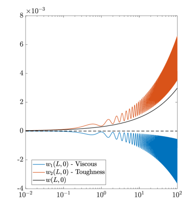
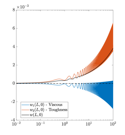
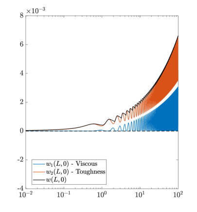
Figure 3: Toughness and viscosity components of the aperture (4) at $x=0$, (a), (b) $\delta_{max}=1$, $\delta_{min}=0.1$, (c), (d) $\delta_{max}=10$, $\delta_{min}=1$, (e), (f) $\delta_{max}=100$, $\delta_{min}=10$.

Stress intensity factor:

$$K_{I}(t)=2\sqrt{\frac{L(t)}{\pi}}\int_{0}^{L(t)}\frac{p(t,s)ds}{\sqrt{L^{2}(t)-s^{2}}},$$ (5)

where $K_{I}(t)$ is the stress intensity factor.
Irwin criterion (fracture criterion from Linear Elastic Fracture Mechanics):

$$K_{I}(t)=K_{IC}(L(t)),\quad t\geq 0,$$ (6)

where $K_{IC}(L(t))$ is the material toughness (see Sect. 2.1.1) local to the crack tip.
Crack opening boundary conditions:

$$q(t,0)=\frac{1}{2}Q_{0}(t).$$ (7)

In addition, the form of operator (4) implies that:

$$\frac{\partial w}{\partial x}(t,0)=0.$$ (8)

Crack tip boundary conditions:

$$w(t,L(t))=0,\quad q(t,L(t))=0.$$ (9)

Fluid velocity:
In addition to these equations we introduce the fluid velocity, $v$, as a new parameter. It describes the average speed of fluid flow through the fracture cross section. This follows from (3) as:

$$v(t,x)=\frac{q(t,x)}{w(t,x)}=-\frac{1}{M^{\prime}}w^{2}\frac{\partial p}{\partial x}.$$ (10)

Provided the fluid front coincides with the crack tip (i.e. no fluid lag and finite fluid leakoff at the tip), the speed equation holds [Linkov, 2011]

$$\frac{dl}{dt}=v(t,L(t))=-\frac{1}{M^{\prime}}w^{2}\frac{\partial p}{\partial x}\bigg{|}_{x=L(t)}.$$ (11)

The advantages of applying this in computations alongside the system asymptotics are well documented, see e.g. [Detournay and Peirce, 2014, Linkov, 2012, Wrobel and Mishuris, 2015]. Crucially for the present analysis, this allows for highly accurate tracing of the fracture front while also ensuring that the fracture velocity is computed as a component of the solution.

2.1.3 Numerical solver for hydraulic fracture of a heterogeneous material

This system of equations is solved utilizing a time-space solver developed by the authors, which is of “universal algorithm” type, see e.g. [Wrobel and Mishuris, 2015, Perkowska et al., 2015, Peck et al., 2018]. The particular algorithm utilized in this paper is the same as that utilized in [Da Fies et al., 2022, Da Fies et al., 2023], while a detailed overview of its construction can be found in [Da Fies, 2020]. The algorithm has been demonstrated to achieve an exceptionally high level of solution accuracy, with the algorithm being computed to a specified level of global solution error. Throughout this paper, the key computational parameters $w$, $v$, $p_{x}$, have a global error below $10^{-4}$ (see e.g. the energy balance relative error presented in Fig. 5). Note however that the local error may be higher, particularly for high toughness ratios (e.g. $\delta_{max}=100$, $\delta_{min}=10$) and the step-wise distribution. More accurate computations were performed where necessary. Checks have been performed to ensure that datasets are computed to a sufficient level of accuracy to verify the stated results. For full details see [Da Fies, 2020].

2.1.4 Material parameters used in computations

The material parameters used in simulations correspond to those typically encountered in hydraulic fracturing of rock (see [Da Fies et al., 2022] and references therein). They are provided in Table. 1.

$E$	$\nu$	$\mu$	$H$	$Q_{0}$
$2.81\times 10^{10}$   [Pa]	$0.25$	$1\times 10^{-3}$   [Pa s]	$15$   [m]	$6.62\times 10^{-2}$   [m3 / s]

Table 1: Problem parameters used in simulations, with $H$ denoting the fracture height. Note that the pumping rate $Q_{0}$ is taken to be constant.

2.2 Monitoring the local fracture regime

The regime of the fracture determines the extent and character of crack propagation (for more details see e.g. [Garagash et al., 2011, Lecampion et al., 2017] and references therein). In its simplest description (and in absence of fluid leak-off), hydraulic fracture propagation is either fluid viscosity or material toughness dominated, with a transient regime in between. Unlike in conventional models, those incorporating heterogeneous toughness may experience “rock-layer”-dependent propagation regimes, which vary rapidly as the crack advances, see e.g. [Da Fies et al., 2022, Da Fies et al., 2023].

Examining the behaviour of such fractures therefore requires outlining a measure with which to estimate the regime of fracture propagation at any given moment. We utilize the measure, denoted $\delta(t)$, first introduced in [Da Fies et al., 2022] to characterise the regime local to the crack tip. As it was investigated in more details there, below we focus only on re-introducing it and briefly discussing its behaviour.

2.2.1 Parameter $\delta$

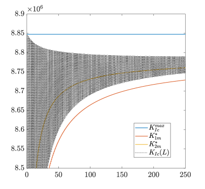
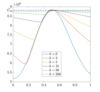
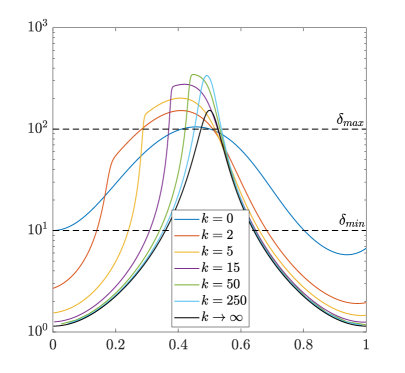
Figure 4: Behaviour of (a), (b) $C(L)$ over $L(t)$ (see (15)), and (c), (d) $C(L)$ and (e), (f) $\delta(L)$ against the value of $L(t)$ within the $k^{\text{th}}$ toughness period for the (a), (c), (e) sinusoidal, (b), (d), (f) piece-wise toughness distribution. Data is taken for the toughness-toughness case ($\delta_{max}=100$, $\delta_{min}=10$). The (assumed constant) limiting value $C\to C_{\infty}$ is $L\to\infty$ is obtained using least-squares, with the limiting behaviour of $\delta$ following from (17). The parameters $K_{1m}^{*}$, $K_{2m}^{*}$ are temporal-averaged values of the toughness, obtained using the formulae from [Da Fies et al., 2022].

As noted in Sect. 2.1.2, the elasticity equation (4) can be expressed as

$$w(t,x)=w_{1}(t,x)+w_{2}(t,x),$$ (12)

where term $w_{1}(t,x)$ describes the effect of the fluid viscosity, while $w_{2}(t,x)$ describes the impact of the material toughness on the fracture profile (shown graphically in Fig. 3). Let us examine the fracture volume, described as

$$V(t)=\int_{0}^{L(t)}w(t,x)dx,\quad V_{j}(t)=\int_{0}^{L(t)}w_{j}(t,x)dx,\quad j=1,2,$$ (13)

$$V(t)=V_{1}(t)+V_{2}(t).$$

In the case of a constant injection rate ($Q_{0}=const$), and where the crack starts from zero length, two of these terms can be computed explicitly (utilizing (2))

$$V(t)=\frac{Q_{0}t}{2H},\quad V_{2}(t)=\sqrt{\pi L(t)}\,\frac{K_{I}(t)}{E^{\prime}}L(t).$$ (14)

This allows us to introduce the following measure, first outlined in [Da Fies et al., 2022], which is given by the ratio of the fluid and toughness associated volumes

$$\delta(t)=\frac{V_{2}(t)}{V_{1}(t)}=\frac{V_{2}(t)}{V(t)-V_{2}(t)}=\frac{K_{Ic}(t)}{C(t)-K_{Ic}(t)},\quad C(t)=\frac{q_{0}E^{\prime}}{2H\sqrt{\pi}}\frac{t}{L^{3/2}(t)},$$ (15)

that describes the local propagation regime at the crack tip: $\delta\ll 1$ corresponds to the viscosity dominated (small toughness) regime, while $\delta\gg 1$ indicates toughness dominated propagation. Note however that this is only intended as an approximate measure. The new parameter $C(t)$, shown in Fig. 4a,b, is useful for modelling and investigating limiting behaviour as $t\to\infty$, as will be discussed in the next section. The values of $\delta(L(t)))$, $C(L(t))$, as the crack propagates through various toughness periods are given in Fig. 4.

To account for the fracturing regime in our investigations, we take the material toughness’ maximum, $K_{Ic}^{max}$, and minimum, $K_{Ic}^{min}$, values to correspond to specific values of $\delta$ (computed for a homogeneous material). These values are given in Table. 2. For example, taking $K_{Ic}^{max}$ corresponding to $\delta=10$, and $K_{Ic}^{min}$ corresponding to $\delta=0.1$, we can investigate a material whose layers alternate between the Toughness and Viscosity dominated regimes respectively. Throughout the paper, we denote the toughness pairing using $\delta_{max}$, $\delta_{min}$, for the sake of simplicity.

${\delta}$	$0.1$	$1$	$10$	$100$
$K_{Ic}$ [Pa $\sqrt{\text{m}}$]	$3.260\times 10^{5}$	$1.860\times 10^{6}$	$4.700\times 10^{6}$	$8.760\times 10^{6}$

Regime	Intermediate - Viscosity	Toughness - Intermediate	Toughness - Toughness
	$\delta_{max}=1$, $\delta_{min}=0.1$	$\delta_{max}=10$, $\delta_{min}=1$	$\delta_{max}=100$, $\delta_{min}=10$

Table 2: (a) Values of the material toughness $K_{Ic}$ (to $3$ s.f.) corresponding to the given value of the ratio $\delta$ (15), for a rock whose other material parameters are as stated in Table. 1. (b) Values of $\delta_{max}$ and $\delta_{min}$ (corresponding to $K_{Ic}^{max}$ and $K_{Ic}^{min}$) used in computations to model different regime combinations.

2.2.2 Behaviour as $L\to\infty$

It has been demonstrated that the solution for heterogeneous toughness will tend to the maximum toughness solution as the crack length tends to infinity [Dontsov and Suarez-Rivera, 2021, Da Fies et al., 2022]. Combining this with results for the long-time asymptotics (see e.g. [Garagash et al., 2011] and references therein), as $t\to\infty$:

$$L(t)=l_{\infty}(Q_{0},\mu,E^{\prime},K_{IC}^{\max})t^{2/3},$$ (16)

for some $l_{\infty}$, which depends upon the process parameters.

Assuming the function $C(t)$ tends to some constant limiting value $C\to C_{\infty}$ as $t\to\infty$ (for discussion of this assumption, see Appendix. A), then combining this representation with the definition of $\delta$ (15) we obtain the limiting behaviour as $t\to\infty$

$$\delta_{\infty}(t)=\frac{K_{Ic}\left(L(t)\right)}{C_{\infty}-K_{Ic}\left(L(t)\right)}.$$ (17)

It is clear that we must have $C_{\infty}>K_{Ic}^{max}$, while in the infinite toughness limit $C_{\infty}\to K_{Ic}^{max}$ as $K_{Ic}^{max}\to\infty$. We also have that, for two periodic toughness distributions $K^{(1)}_{IC}(x)$ and $K^{(2)}_{IC}(x)$ such that $K^{(1)max}_{IC}=K^{(2)max}_{IC}$, and $K^{(1)}_{IC}(x)\geq K^{(2)}_{IC}(x)$, then $\delta_{\infty}^{(1)max}=\delta_{\infty}^{(2)max}$ and $\delta_{\infty}^{(1)}(x)\geq\delta_{\infty}^{(2)}(x)$.

$\delta_{max}-\delta_{min}$	$1-0.1$	$10-1$	$100-0.1$	$100-1$	$100-10$
$C_{\infty}$ [Pa $\sqrt{\text{m}}$]	$3.690\times 10^{6}$	$5.131\times 10^{6}$	$8.806\times 10^{6}$	$8.813\times 10^{6}$	$8.816\times 10^{6}$
$C_{\infty}$ for $K_{Ic}\equiv K_{1m}^{*}$ [Pa $\sqrt{\text{m}}$]	$3.690\times 10^{6}$	$5.118\times 10^{6}$	$8.790\times 10^{6}$	$8.798\times 10^{6}$	$8.799\times 10^{6}$
$C_{\infty}$ for $K_{Ic}\equiv K_{2m}^{*}$ [Pa $\sqrt{\text{m}}$]	$3.699\times 10^{6}$	$5.130\times 10^{6}$	$8.792\times 10^{6}$	$8.805\times 10^{6}$	$8.806\times 10^{6}$
$C_{\infty}$ for $K_{Ic}\equiv K_{Ic}^{max}$ [Pa $\sqrt{\text{m}}$]	$3.723\times 10^{6}$	$5.170\times 10^{6}$	$8.848\times 10^{6}$	$8.848\times 10^{6}$	$8.848\times 10^{6}$
$K_{Ic}^{max}$ [Pa $\sqrt{\text{m}}$]	$1.860\times 10^{6}$	$4.700\times 10^{6}$	$8.760\times 10^{6}$	$8.760\times 10^{6}$	$8.760\times 10^{6}$

$\delta_{max}-\delta_{min}$	$1-0.1$	$10-1$	$100-0.1$	$100-1$	$100-10$
$C_{\infty}$ [Pa $\sqrt{\text{m}}$]	$3.711\times 10^{6}$	$5.158\times 10^{6}$	$8.842\times 10^{6}$	$8.843\times 10^{6}$	$8.843\times 10^{6}$
$C_{\infty}$ for $K_{Ic}\equiv K_{1m}^{*}$ [Pa $\sqrt{\text{m}}$]	$3.689\times 10^{6}$	$5.151\times 10^{6}$	$8.828\times 10^{6}$	$8.830\times 10^{6}$	$8.832\times 10^{6}$
$C_{\infty}$ for $K_{Ic}\equiv K_{2m}^{*}$ [Pa $\sqrt{\text{m}}$]	$3.700\times 10^{6}$	$5.158\times 10^{6}$	$8.830\times 10^{6}$	$8.836\times 10^{6}$	$8.842\times 10^{6}$
$C_{\infty}$ for $K_{Ic}\equiv K_{Ic}^{max}$ [Pa $\sqrt{\text{m}}$]	$3.723\times 10^{6}$	$5.170\times 10^{6}$	$8.848\times 10^{6}$	$8.848\times 10^{6}$	$8.848\times 10^{6}$
$K_{Ic}^{max}$ [Pa $\sqrt{\text{m}}$]	$1.860\times 10^{6}$	$4.700\times 10^{6}$	$8.760\times 10^{6}$	$8.760\times 10^{6}$	$8.760\times 10^{6}$

Table 3: Values of $C_{\infty}$ (17) obtained for material toughness regimes $K_{Ic}(L)$ with the (a) sinusoidal, (b) step-wise, distribution. Here $K_{1m}^{*}$, $K_{2m}^{*}$, are the values of the ’average’ material toughness obtained using the temporal-averaging strategy outlined in [Da Fies et al., 2022].

The behaviour of $C(t)$ and $\delta(t)$, alongside the limiting behaviour as $t\to\infty$, are provided in Fig. 4. The limiting value $C_{\infty}$ is also shown, with the values for various toughness distributions provided in Table. 3, alongside those for the heterogeneous case with $K_{Ic}(L)\equiv K_{Ic}^{max}$. The values predicted by the temporal-averaged toughness $K_{Ic}(L)\equiv K_{1,2m}^{*}$ from [Da Fies et al., 2022] are also included. The method by which these values were obtained is outlined in Appendix. A, with the behaviour of $\delta_{\infty}$ following from (17).

From Table. 3, we can see that the rock heterogeneity does play a role in the limiting behaviour. The values of $C(L)$ for the heterogeneous toughness distribution do not converge to those of the maximum toughness $K_{Ic}\equiv K_{Ic}^{max}$ as $L\to\infty$, with $C_{\infty}(K_{Ic}(L))<C_{\infty}(K_{Ic}^{max})$ in all cases. The temporal-averaging based approaches from [Da Fies et al., 2022] are effective at predicting the limiting value $C_{\infty}$ for all considered distributions, with the energy-based average $K_{2m}^{*}$ being a better predictor than $K_{1m}^{*}$. Meanwhile, the particular toughness distribution also influences the result, with the value of $C_{\infty}$ for the square distribution always being larger than that for the sinusoidal distribution. Finally, comparing the results when $\delta_{max}-\delta_{min}$ are $100-1$ and $100-10$, we can see that the minimum toughness only plays a minor role in the value of $C_{\infty}$ compared to that of the maximum toughness.

3 Energy distribution during heterogeneous fracture

As a hydraulic fracture propagates within a heterogeneous material the extent of ‘viscosity’ and ‘toughness’-dominated behaviour is amplified. This can be seen from the behaviour of $\delta$ in Fig. 4c,d, with the maximum of $\delta$ noticeably exceeding $\delta_{max}$, and the minimum of $\delta$ being almost an order of magnitude below $\delta_{min}$.

In the preceding work [Da Fies et al., 2022] (and by others, see that paper), an explanation of this was given in terms of the fracture pressurisation. To obtain a fuller picture however, we need to examine the system behaviour from an energy perspective.

3.1 Overview of the energy distribution

Figure 5: The global (cumulative) relative error of numerical computations for the energy components against (propagation) time, computed from (18), for the (a) sinusoidal and (b) step-wise toughness distributions.

In order to investigate the physical processes occurring within the hydraulic fracture, we consider the energy balance within the fracture over time. In the case of a single hydraulic fracture propagating without fluid lag, the energy within the fracture at each moment in time consists of four primary terms:

• The power, $P(L)$, representing the energy added to the system due to fluid injection.

• The toughness energy, $S(L)$, representing the energy spent fracturing the solid material.

• The viscous energy, $D(L)$, stored within the fluid.

• The elastic energy, $U(L)$, stored within the solid material.

For details on the derivation of these terms within a hydraulic fracture see for example [Lecampion and Detournay, 2007, Bunger, 2013] and references therein. The formulae given below are adapted from those provided in [Bunger, 2013].

These four energy terms in the case of a single fracture without fluid lag are related as

$$P(L)=D(L)+S(L)+U(L).$$ (18)

where each energy term is given by:

$$P(L)=2p(0,t)q(0,t),\quad D(L)=\frac{1}{M^{\prime}}\int_{0}^{L(t)}w\left(\frac{\partial p}{\partial x}\right)^{2}\,dx=M^{\prime}\int_{0}^{L(t)}\frac{v^{2}(t,x)}{w(t,x)}\,dx,$$ (19)

$$S(L)=\frac{2}{E^{\prime}}v_{0}(t)K_{Ic}^{2}\left(L(t)\right),\quad U(L)=\int_{0}^{L(t)}p\frac{\partial w}{\partial t}+w\frac{\partial p}{\partial t}\,dx=\int_{0}^{L(t)}\frac{\partial}{\partial t}\left(p(t,x)w(t,x)\right)\,dx.$$

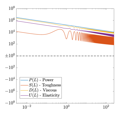
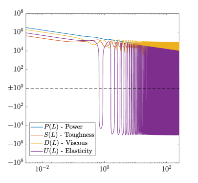
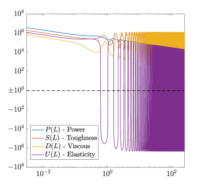
Figure 6: Distribution of the power [W] (19) within the hydraulic fracture as it propagates through the domain. This is for the (a), (b) intermediate-viscosity, (c), (d) toughness-intermediate, (e), (f) toughness-toughness, case with the (a), (c), (e) sinusoidal, (b), (d), (f) step-wise, toughness distribution.

In the numerical solver, each of these terms is computed separately during post-processing from the system parameters. Consequently, the accuracy of the energy computations can be inferred using (18), with the global (cumulative) relative error of this expression provided in Fig. 5. The solver is run to a prescribed tolerance, with the default setting ensuring that the error in the crack tip velocity remains below $10^{-4}$ at each time-step. As can be seen in Fig. 5, the relative error of the total energy is of the same order throughout the simulations. This however can still mean sharp spikes in the local error, particularly when the difference between the maximum and minimum toughness is large (e.g. $\delta_{max}=100,\delta_{min}=10$), and over long simulated time-scales. On the other hand, taking a stricter tolerance for the crack tip velocity improves the local energy balance, while the relative difference in results for the physical parameters (crack length, velocities, pressure) remains below the original threshold.

This however remains sufficiently accurate to verify the claims made in this paper. With this we can examine how the energy balance impacts the propagation of fracture within a heterogeneous material.

3.2 Energy distribution and the elastic battery

Figure 7: Distribution of the power [W] (19) within the hydraulic fracture as it propagates through the $250^{\text{th}}$ toughness period. This is for the intermediate-viscosity case ($\delta_{max}=1$, $\delta_{min}=0.1$) with the (a), sinusoidal, (b) step-wise, toughness distribution. Recall that for the stepwise distribution, $0.25<L-kX<0.75$ corresponds to the maximum toughness layer, with the remainder of the domain corresponding to the minimum toughness layer.

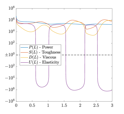
Figure 8: Distribution of the power [W] (19) within the hydraulic fracture as it propagates through (a), (b) the first three toughness periods, and the $k^{\text{th}}$ toughness period with (c), (d) $k=250$. This is for the toughness-toughness case ($\delta_{max}=100$, $\delta_{min}=10$) with the (a), (c) sinusoidal, (b), (d) step-wise, toughness distribution. Recall that for the stepwise distribution, $0.25<L-kX<0.75$ corresponds to the maximum toughness layer, with the remainder of the domain corresponding to the minimum toughness layer.

To more easily examine the data, we make a change of coordinate system to examine $(x,L(t))$. As $L(t)$ represents the crack length, and hence the layer of material the crack is propagating through at time $t$, this change allows us to examine the dependence of the energy on the toughness of the material being propagated through at each specific moment. This is also necessary to make the analysis easier, as the exceptionally rapid propagation of the fracture through weaker material layers (i.e. reaching propagation velocities of almost $100$m/s in the toughness-toughness case, see Fig. 11), means that effects occurring during propagation through weaker layers would be almost imperceptible without rescaling.

Figures showing the energy distribution (19) as the fracture propagates through the heterogeneous material are provided in Fig. 6, while a comparison of the energy terms within a single toughness period are given in Figs. 7-8. Additional figures showing the energy distribution for all cases are in the supplementary material (Figs. B.1-B.3). It can be seen that, after the initial two periods, the energy distribution settles into a periodic oscillation to match the toughness, with only small changes over time.

With at least one layer in the toughness dominated regime

• As can be seen clearly in Fig. 8, while propagating in the maximum toughness layer, the ‘power’ being injected into the fracture is stored within the elastic material - with far less being used to propagate the fracture, resulting in a slower propagation rate.

• Once the fracture reaches the minimum toughness layer, this elastic energy is rapidly transferred to both the fracture propagation and the fluid.

This behaviour is observed in both the toughness-toughness and toughness-intermediate cases (see Fig. 6, also Figs. B.1-B.3), indicating that the presence of a ’toughness-dominated’ layer is the key factor for initiating this behaviour.
With all layers in the viscosity dominated/ intermediate regime

• If both layers are in the viscosity dominated regime then the energy distribution is largely independent of the material toughness. Storage within the elastic material does however play a significant role over long length-scales, due to the abundance of elastic material, however this is dependent on the toughness distribution (compare Fig. 7a,b).

These behaviours explain the rapid fracture propagation through the weaker material. However, this also induces more fundamental changes in the fracture geometry. These can be seen most clearly be examining the fracture aperture at the point of injection $x=0$, provided in Fig. 9a,b, which can be seen to oscillate as the crack passes between high and low toughness layers. In this way, the elastic medium behaves as a battery, storing energy while propagating through tougher material, and then releasing it during propagation through the weaker layers. Corresponding oscillations can also be seen in the fluid velocity and pressure, as shown in Figs. 9c-f, and for the fluid velocity throughout the crack length in Fig. 11.

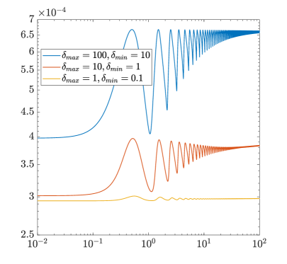
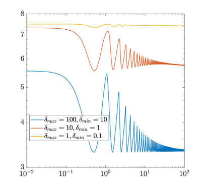
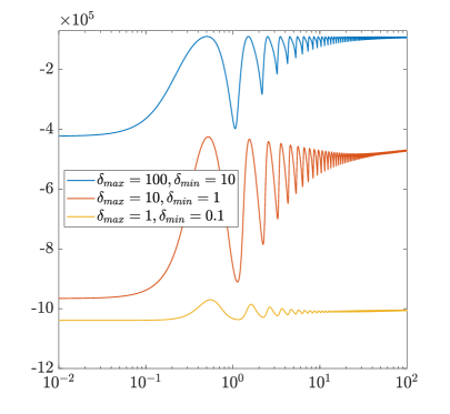
Figure 9: The (a), (b) normalised aperture $w(L(t),x)/\sqrt{L(t)}$, (c), (d) normalised fluid velocity $\sqrt{L(t)}v(L(t),x)$, (e), (f) normalised fluid pressure derivative $L^{3/2}(t)p_{x}(L(t),x)$, at the fracture opening $x=0$ as the crack propagates through the heterogeneous material whose periodic toughness has a (a), (c), (e) sinusoidal, (b), (d), (f) step-wise, distribution.

3.3 Limiting behaviour of the energy distribution

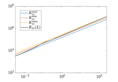
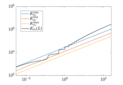
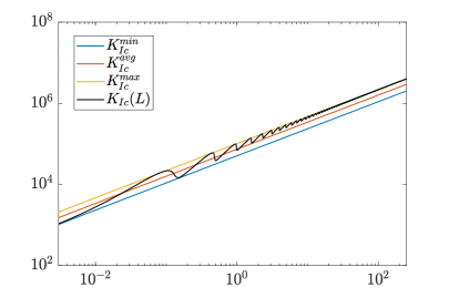
Figure 10: The cumulative energy terms (19) for the toughness-toughness case with (a), (c), (e), (g) sinusoidal, (b), (d), (f), (h) step-wise, distribution. These are shown alongside the behaviour for the case of homogeneous toughness with distributions: maximum toughness $K_{Ic}(L)\equiv K_{Ic}^{max}$, minimum toughness $K_{Ic}(L)\equiv K_{Ic}^{min}$, and the (arithmetic) average toughness $K_{Ic}(L)\equiv K_{Ic}^{avg}$. Here $P$ is the power injected into the fracture, $S$ the toughness (propagation energy), $D$ the viscous energy (stored in the fluid), and $U$ the elastic energy (stored in the solid).

With the instantaneous energy distribution considered, let us now investigate the limit behaviour. To do this, we consider the cumulative energy for each term, and compare it against the behaviour expected for fracture in a homogeneous material with the toughness equal to: the maximum toughness $K_{Ic}(L)\equiv K_{Ic}^{max}$, the minimum toughness $K_{Ic}(L)\equiv K_{Ic}^{min}$, and the (arithmetic) average toughness $K_{Ic}(L)\equiv K_{Ic}^{avg}=0.5\left(K_{Ic}^{max}+K_{Ic}^{min}\right)$.

As the viscosity-dominated case has cumulative behaviour that is largely independent of the toughness distribution, the figures for these cases are relegated to the supplementary material (Figs. B.4-B.7). Meanwhile, figures showing the toughness-toughness case ($\delta_{max}=100$, $\delta_{min}=10$) are provided in Fig. 10.

With all layers are in the viscosity dominated/ intermediate regime

• In this case, only the toughness energy $S$ shows significant differences in behaviour between the different toughness distributions, with the cumulative behaviour for the oscillating toughness case being close to, but slightly above, that of the average toughness (see Figs. B.4-B.7).

With both layers in the toughness-dominated regime
There is a clear difference in limiting behaviour between the different energy terms (see Fig. 10).

• For the power $P$ and elastic energy $U$ the oscillating (periodic) toughness tends to that of the maximum $K_{Ic}^{max}$.

• The toughness term meanwhile tends to that of the (arithmetic) average $K_{Ic}^{avg}$.

• To balance this, the viscous energy (stored in the fluid) $D$ exceeds that for all cases, tending to something visibly above the maximum.

• There is no apparent dependence on the form of the toughness distribution, with both the sinusoidal and step-wise toughness distributions providing almost identical results.

Similar results are found for the toughness-intermediate case (see Figs. B.4-B.7), with $P$, $U$, tending to a value slightly below that for the maximum $K_{Ic}^{max}$, and $S$ again tending to that for the (arithmetic) average. The main difference is that $D$ does not need to go above the maximum to balance the other terms, and thus tends to a value slightly below the maximum.

4 Velocity of the fluid and the crack tip

With the energy distribution considered, let us now examine the velocity and acceleration of the crack tip, as well as that of the fluid within the fracture.

4.1 Crack tip propagation

As the fluid front and crack tip coincide (due to the no-lag assumption), we show graphically only the more general case of the fluid velocity throughout the fracture. These are provided in Fig. 11, for various normalised positions within the crack $\tilde{x}=x/L$. The case $\tilde{x}=1$ therefore coincides with the velocity of the crack front. The associated fluid acceleration is meanwhile relegated to the supplementary material (Fig. B.8).

As expected, Fig. 11 shows that the fracture rapidly propagates through the weaker material, while it slows as it permeates the tougher material, leading to rapid velocity oscillations. Comparing the various cases, it can be seen that the oscillations are far greater in the toughness-toughness case than the intermediate-viscosity one, with the former’ crack tip experiencing both the fastest and slowest velocities of any case shown here. Comparisons by the authors (keeping $\delta_{max}=100$ and taking $\delta_{min}=10,1,0.1$) found that the extent of these oscillations primarily depends upon the maximum toughness, rather than the difference between the maximum and minimum toughness, although the latter does play a small role.

The toughness distribution meanwhile does have some impact, with the variations in the velocity being larger for the step-wise case than the sinusoidal one. The main impact of the toughness distribution however is on the acceleration of the crack front, as seen in Fig. B.8 (with $\tilde{x}=1$). It is apparent from those figures that the step-wise distribution experiences a peak acceleration that is consistently higher than that of the sinusoidal one. For example, in the toughness-toughness case ($\delta_{max}=100,\delta_{min}=10$) the peak acceleration of the step-wise distribution exceeds $10^{5}$ m/s², which is an order of magnitude greater than that of the sinusoidal one. This trend holds for all of the cases considered here, with the acceleration in the step-wise case always being an order or more greater than that for the sinusoidal distribution.

4.2 Fluid velocity within the fracture: the backflow effect

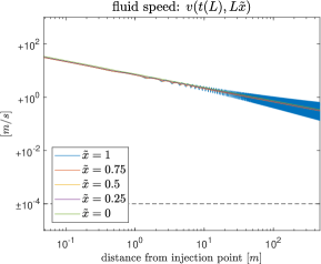
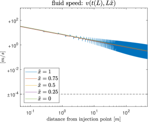
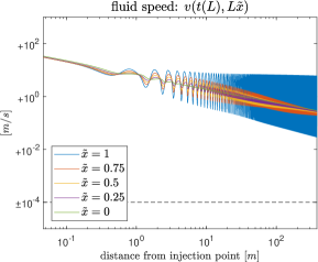
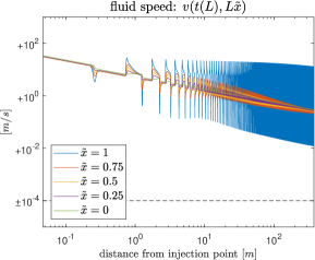
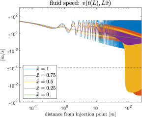
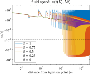
Figure 11: Fluid velocity inside the fracture for KGD for 5 chosen positions (beginning and the end of the fracture and at each quarter of the length). Note that the points move in time. (a), (b) $\delta_{max}=1$, $\delta_{min}=0.1$, (c), (d) $\delta_{max}=10$, $\delta_{min}=1$, (e), (f) $\delta_{max}=100$, $\delta_{min}=10$.

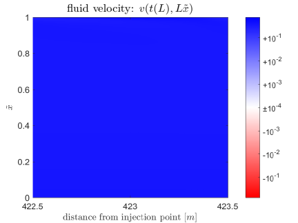
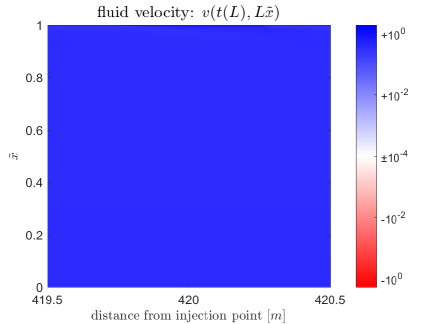
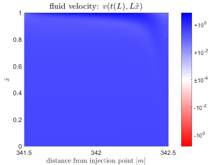
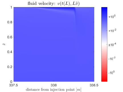
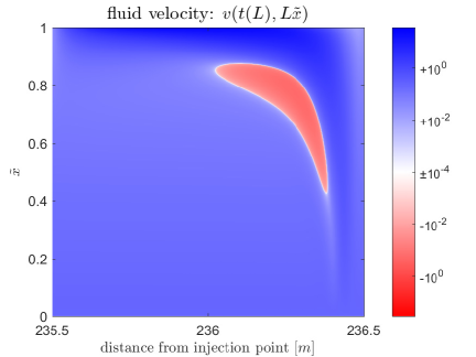
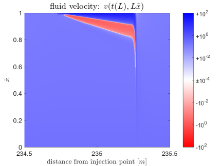
Figure 12: Plots showing the fluid velocity within a single period. (a), (b) $\delta_{max}=1$, $\delta_{min}=0.1$, (c), (d) $\delta_{max}=10$, $\delta_{min}=1$, (e), (f) $\delta_{max}=100$, $\delta_{min}=10$.

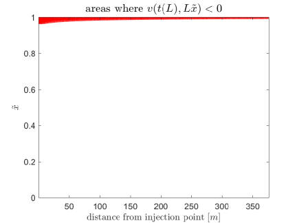
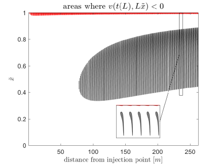
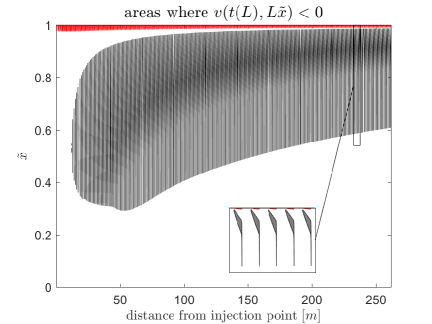
Figure 13: Plots showing negative velocity. (a), (b) $\delta_{max}=10$, $\delta_{min}=1$, (c), (d) $\delta_{max}=100$, $\delta_{min}=10$. The regions coloured red denote the portion near to the crack tip where the pressure derivative is negative.

With the propagation of the crack tip considered, let us now consider the velocity of the fluid inside the fracture. The fluid velocity within the fracture for fixed normalised spacial positions $\tilde{x}=x/L$ are again shown in Fig. 11, while the fluid acceleration is relegated to the supplementary material (Fig. B.8).

We can see that in the intermediate-viscosity and toughness-intermediate cases there is a very similar trend for the fluid velocity as was seen for the crack tip velocity (and crack opening $x=0$, see Fig. 9c,d). Namely, the fluid velocity oscillates as the crack propagates between weaker and tougher layers. This effect reduces away from the crack tip and almost disappears at the fracture opening $x=0$. However, the extent to which this is the case varies depending on whether the crack is (locally) in the viscosity or toughness dominated regimes.

Examining the toughness-toughness case however, we can see a significantly different behaviour occurring between the fracture front and midpoint. Namely, while behaving similarly to the previous cases during initial propagation (until $L\approx 50$), after this point the fluid velocity begins to ’backflow’ upon encountering weaker material layers. This can clearly be seen in Figs. 11e,f, where the fluid velocity at $\tilde{x}=0.5,0.75$ is negative, and of order $10^{0}$, when transitioning from the tougher material layers to the weaker ones.

We focus in more detail on the region of the fracture where this backflow occurs. In Fig. 12 we show on the behaviour within a single toughness period. We can see that the extent of the backflow effect is strongly dependent on the maximum toughness, with there being a strong backflow effect in the toughness-toughness case, but in the toughness-intermediate case there are only regions of fluid stagnation (without backflow). These effects are entirely absent in the intermediate-viscosity case, for which fluid always travels towards the crack tip. Note however that the backflow is in part dependent on the toughness distribution, occurring in a different portion of the crack for the step-wise and sinusoidal distributions.

In 13 we can see that this behaviour is mirrored throughout the later periods of fracture propagation, rather than an isolated effect. The toughness distribution plays a crucial role here, with the step-wise (layered) distribution exhibiting the backflow effect after a far shorter propagation distance (time), and over a far wider portion of the crack, than the sinusoidal toughness distribution.

This backflow effect is physical, and has been replicated by others whose solvers are based on significantly differing assumptions. Crucially, this phenomena can be explained in terms of the elastic battery outlined in Sect. 3.2. The crack geometry changes as it transitions from propagating in a tougher material to a weaker one. Notably, the aperture decreases throughout the crack. The resulting redistribution of fluid is the most likely cause of the backflow effect.

5 Discussions and Conclusions

Essential features of HF propagation in media with heterogeneous fracture toughness were investigated. A ‘universal solver’-type algorithm was implemented to provide high accuracy results for the fracture growth, profile and energy distribution. The key findings are as follows.

• Limiting behaviour: A new parameter $C_{\infty}$ was introduced to describe the limiting regime of a hydraulic fracture through heterogeneous media as crack length $L\to\infty$. This value, provided it is constant (see analysis in Appendix. A), can be used to quantify the impact of the heterogeneity on the crack behaviour. Crucially, the value of $C_{\infty}$ for oscillating toughness $K_{Ic}(L)$ does not converge to that for the maximum toughness $K_{Ic}^{max}$, and is dependent on the toughness distribution (i.e. sinusoidal or step-wise).

• Energy distribution: The energy distribution within a hydraulic fracture travelling through heterogeneous rock was investigated. The four primary terms, the power, toughness, viscous and elastic energy were evaluated for the case of periodic toughness distribution with a step-wise and sinusoidal (infinitely layered) distribution.

• Elastic battery: It was demonstrated that the solid media acts as an elastic battery. Elastic energy is stored during propagation through tougher layers, before being rapidly released to the fluid and to drive crack propagation once the crack tip reaches a weaker layer. This elastic battery phenomena was most pronounced when the maximum material toughness promoted toughness-dominated behaviour, but was still present over long length-scales for viscosity-dominated fractures.

• Oscillation of the crack tip velocity: As previously observed, there were rapid changes in fracture velocity during propagation through differing toughness layers. This follows from the elastic battery phenomena, which also describes more fundamental changes in crack geometry (e.g. the crack aperture).

• Fluid backflow: A certain fraction of the fluid volume inside the crack moved in the opposite direction to the crack tip motion. This effect was dependent on the toughness distribution, with backflow occurring at differing times for step-wise and sinusoidal toughness distributions, and the extent (or existence) of backflow depending on the maximum toughness of the material.

The presented work provides physical explanations for observed phenomena. It also predicts new phenomena caused by the heterogeneity. For example, the fluid backflow may lead to sediment redistribution during fracking operations, increasing the likelihood of blockages during flowback operations. The elastic battery phenomenon meanwhile indicates that the likelihood of crack arrest following injection shut-in (see e.g. [Möri and Lecampion, 2021]) should strongly depend on the toughness of the rock-layer at the time fluid injection ceases. Furthermore, as only Newtonian fluid was considered in this work, the impact of the fracturing fluid on the elastic battery is left unanswered; with it possible that it occurs even for dry cracks. More targeted investigations are required to quantify such effects.

Meanwhile, the results for the crack tip velocity oscillation and the fluid backflow are physical effects arising from the change in crack geometry during fracture propagation. These results, and in particular the extreme acceleration of the fluid when propagating between material layers, raises immediate questions about the validity of neglecting the inertia term in the governing equations (1)-(2). Incorporation of this term may well dampen the oscillations seen for the acceleration of the crack tip in heterogeneous media, and lead to qualitative differences in the evolution of the fracture geometry over time. The energy balance may also be impacted by the incorporation of the kinetic energy term.

CRediT authorship contribution statement

Daniel Peck analysis of results, visualisation, produced the manuscript. Gaspare Da Fies produced results for KGD in heterogeneous media, performed initial analysis, initial visualisation. Ivan Virshylo analysis of results, reviewed/edited the manuscript. Gennady Mishuris oversaw all research, analysis of results, reviewed/edited the manuscript.

Appendix A The limiting value $C_{\infty}$

To investigate the limiting value of the parameter $C(L(t))$ (15) as $L\to\infty$, we first extract the minimum and maximum values of the parameter within each period, denoted $C^{min}(L)$ and $C^{max}(L)$ respectively. Examples of these can be seen in Fig. A.1. Determining whether $C(L)\to C_{\infty}$, some constant, as $L\to\infty$ is now equivalent to demonstrating that $C^{min}(L)$ and $C^{max}(L)$ have the same limiting value as $L\to\infty$.

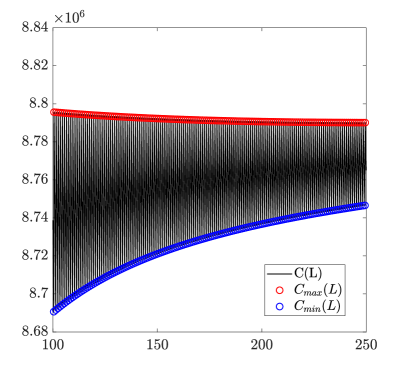
Figure A.1: The value of $C(L(t))$ (15), alongside the distribution of its maximum within each period $C^{max}(L(t))$ and minimum $C^{min}(L(t))$ when $\delta_{max}=100$, $\delta_{min}=10$ for the (a) sinusoidal, (b) step-wise, toughness distribution.

To investigate the limits of the two distributions $C^{max}$ and $C^{min}$, we utilize the least-squares method. We first seek to approximate each of these in the form

$$C^{max/min}(L_{k})=C_{\infty}^{max/min}+AL_{k}^{n}+BL_{k}^{2n},$$ (A.1)

where $C_{\infty}$, $A$, $B$, and $n$ are computed to obtain the approximation. These are obtained separately for $C^{max}(L)$ and $C^{min}(L)$. The limiting values $C_{\infty}^{max}$ and $C_{\infty}^{min}$ are then compared, with their relative differences given in Table. A.1. It can be seen that the relative differences are small in almost all cases, although it does exceed $10^{-1}$ in one instance (sinusoidal distribution with $\delta_{max}-\delta_{min}$ being $10-1$).

While it is not possible to conclude whether the values converge to the same constant $C_{\infty}^{max},C_{\infty}^{min}\to C_{\infty}$ (and therefore $C(L)\to C_{\infty}$ as $L\to\infty$ in general), at minimum because different values can be obtained depending on the assumed distribution, we can state from the above that this will be a reasonable approximation in the cases considered.

Finally, if we assume that $C(L)\to C_{\infty}$ as $L\to\infty$, then we compute $C_{\infty}$ using a combination of both distributions. Namely, noting that all the distributions previously could be approximated taking $n=-0.5$

$$\left\{\begin{array}[]{l}C^{max}(L_{i})=C_{\infty}+AL_{i}^{-\frac{1}{2}}+BL_{i}^{-1},\\ C^{min}(L_{j})=C_{\infty}+DL_{j}^{-\frac{1}{2}}+EL_{j}^{-1},\end{array}\right.$$

$$\therefore\,\sum_{i}\left(C^{max}(L_{i})-C_{\infty}-AL_{i}^{-\frac{1}{2}}-BL_{i}^{-1}\right)^{2}+\sum_{j}\left(C^{min}(L_{j})-C_{\infty}-DL_{j}^{-\frac{1}{2}}-EL_{j}^{-1}\right)^{2}=0.$$

The values of $C_{\infty}$ provided in Table. 3 were obtained using this least-squares approximation applied to the final $50$ toughness periods (to avoid early-time behaviour impacting the long-time approximation). The parameter $\delta_{\infty}$ then follows immediately from (17).

$\delta_{max}-\delta_{min}$	$1-0.1$	$10-1$	$100-1$	$100-10$
Sinusoidal	$6.11\times 10^{-3}$	$1.44\times 10^{-1}$	$1.07\times 10^{-3}$	$6.46\times 10^{-2}$
Square	$1.18\times 10^{-2}$	$3.00\times 10^{-4}$	$7.45\times 10^{-3}$	$2.64\times 10^{-2}$

Table A.1: Relative difference between $C_{\infty}^{max}$ and $C_{\infty}^{min}$ obtained using the least-squares approximation (A.1) (to 2s.f.).

Appendix B Figures

For the sake of readability, not all figures were included in the main text. Here, we include the remaining figures, alongside some brief discussion.

Power distribution as the hydraulic fracture propagates through the rock layers, discussed in the main text in Sect. 3.2, are provided in Figs. B.1-B.3. Note that some figures are repetitions of those given in the main text in Figs. 7,8, but are repeated here for ease of comparison. These figures clearly reinforce the conclusions stated in the main text, namely: the energy terms enter into a periodic oscillation to match the toughness after the first two periods; and the solid domain ‘stores’ elastic energy during propagation through tougher layers, releasing it during propagation through weaker layers (the elastic battery). The latter effect is present in both the toughness-intermediate and toughness-toughness cases, but is only significant for the intermediate-viscosity toughness distribution over long length-scales.

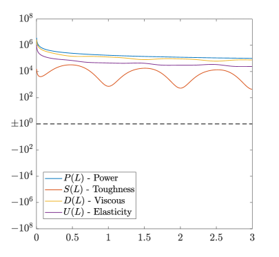
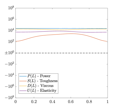
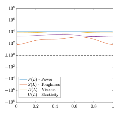
Figure B.1: Distribution of the power [W] (19) within the hydraulic fracture as it propagates through (a), (b) the first three toughness periods, and the $k^{\text{th}}$ toughness period with (c), (d) $k=50$, (e), (f) $k=250$. This is for the intermediate-viscosity case ($\delta_{max}=1$, $\delta_{min}=0.1$) with the (a), (c), (e) sinusoidal, (b), (d), (f) step-wise, toughness distribution. Recall that for the stepwise distribution, $0.25<L-kX<0.75$ corresponds to the maximum toughness layer, with the remainder of the domain corresponding to the minimum toughness layer.

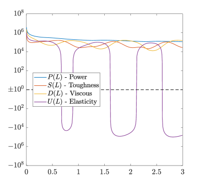
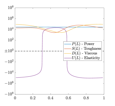
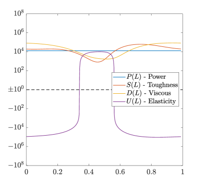
Figure B.2: Distribution of the power [W] (19) within the hydraulic fracture as it propagates through (a), (b) the first three toughness periods, and the $k^{\text{th}}$ toughness period with (c), (d) $k=50$, (e), (f) $k=250$. This is for the toughness-intermediate case ($\delta_{max}=10$, $\delta_{min}=1$) with the (a), (c), (e) sinusoidal, (b), (d), (f) step-wise, toughness distribution. Recall that for the stepwise distribution, $0.25<L-kX<0.75$ corresponds to the maximum toughness layer, with the remainder of the domain corresponding to the minimum toughness layer.

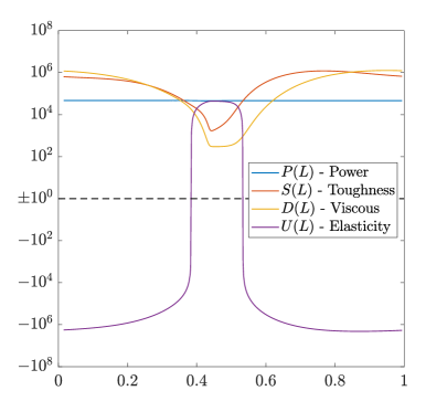
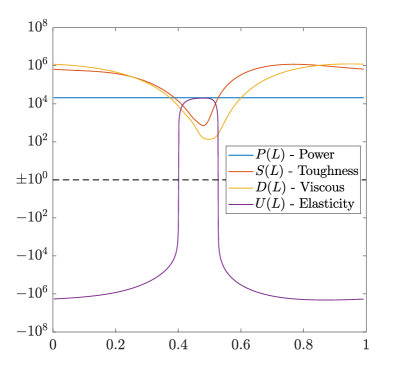
Figure B.3: Distribution of the power [W] (19) within the hydraulic fracture as it propagates through (a), (b) the first three toughness periods, and the $k^{\text{th}}$ toughness period with (c), (d) $k=50$, (e), (f) $k=250$. This is for the toughness-toughness case ($\delta_{max}=100$, $\delta_{min}=10$) with the (a), (c), (e) sinusoidal, (b), (d), (f) step-wise, toughness distribution. Recall that for the stepwise distribution, $0.25<L-kX<0.75$ corresponds to the maximum toughness layer, with the remainder of the domain corresponding to the minimum toughness layer.

The cumulative energy distribution, discussed in the main text in Sect. 3.3, is provided in Figs. B.4-B.7. The comparable figure in the main text is given in Fig. 10, providing all energy terms $P,D,S,U$ for the case $\delta_{max}=100$, $\delta_{min}=10$. Here, we provide each energy term separately and for all three toughness ratios considered in this paper.

These figures include the cumulative energy distribution for oscillating toughness $K_{Ic}(L)$, alongside the cases with homogeneous toughness $K_{Ic}(L)\equiv K_{Ic}$ as:

$$K_{Ic}^{max}=\max_{L\in[0,X]}\left(K_{Ic}(L)\right),\quad K_{Ic}^{min}=\min_{L\in[0,X]}\left(K_{Ic}(L)\right)\quad K_{Ic}^{avg}=\frac{1}{2}\left(K_{Ic}^{min}+K_{Ic}^{max}\right).$$

As stated in the main text:

• In the intermediate-viscosity case, the cumulative energy terms related to the power $P$ (injected into the crack), toughness $D$ (spent extending the fracture), and elasticity $U$ (stored in the solid), show minimal variation between different toughness distributions (i.e. $K_{Ic}(L)\equiv K_{Ic}^{max}$, etc). It is therefore only the viscous term $S$ (energy stored in the fluid) that varies significantly with the toughness distribution, and this tends to that of the (arithmetic) average toughness.

• For cases with at least one layer in the toughness dominated regime, the power $P$ and elastic $U$ energy terms tend to that for the maximum toughness $K_{Ic}(L)\equiv K_{Ic}^{max}$, while the viscous term $S$ tends to that for the (arithmetic) average $K_{Ic}\equiv K_{Ic}^{avg}$. The toughness term $D$, spent extending the fracture, then takes the value needed to maintain the energy balance (18), resulting in a limiting value above those for all considered homogeneous cases for the toughness-toughness distribution (see Fig. B.5e,f).

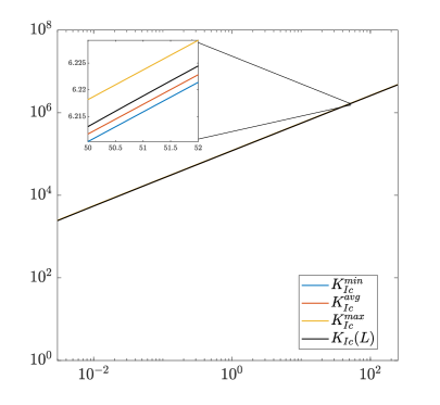
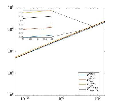
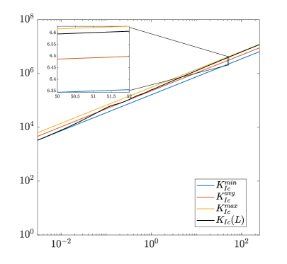
Figure B.4: The cumulative power injected into the fracture $P$, (19), alongside the behaviour for the case of homogeneous toughness with distributions: maximum toughness $K_{Ic}(L)\equiv K_{Ic}^{max}$, minimum toughness $K_{Ic}(L)\equiv K_{Ic}^{min}$, and the (arithmetic) average toughness $K_{Ic}(L)\equiv K_{Ic}^{avg}$. We consider toughness distributions (a), (b) $\delta_{max}=1$, $\delta_{min}=0.1$, (c), (d) $\delta_{max}=10$, $\delta_{min}=1$, (e), (f) $\delta_{max}=100$, $\delta_{min}=10$, in the (a), (c), (e) sinusoidal, (b), (d), (f) step-wise, cases.

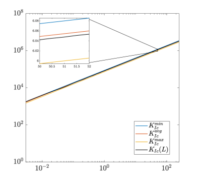
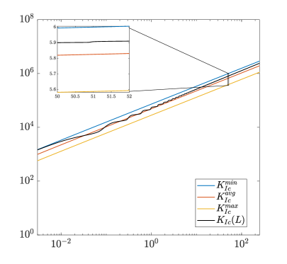
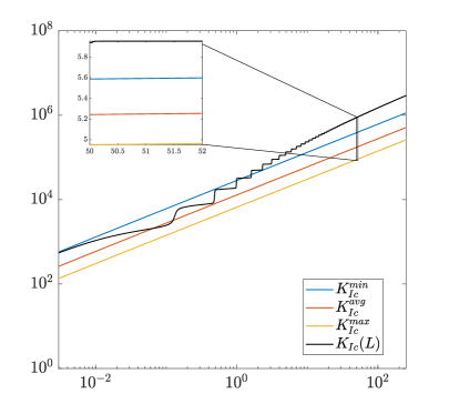
Figure B.5: The cumulative viscous energy stored within the fluid $D$, (19), alongside the behaviour for the case of homogeneous toughness with distributions: maximum toughness $K_{Ic}(L)\equiv K_{Ic}^{max}$, minimum toughness $K_{Ic}(L)\equiv K_{Ic}^{min}$, and the (arithmetic) average toughness $K_{Ic}(L)\equiv K_{Ic}^{avg}$. We consider toughness distributions (a), (b) $\delta_{max}=1$, $\delta_{min}=0.1$, (c), (d) $\delta_{max}=10$, $\delta_{min}=1$, (e), (f) $\delta_{max}=100$, $\delta_{min}=10$, in the (a), (c), (e) sinusoidal, (b), (d), (f) step-wise, cases.

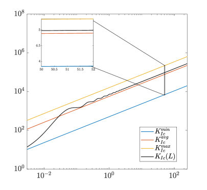
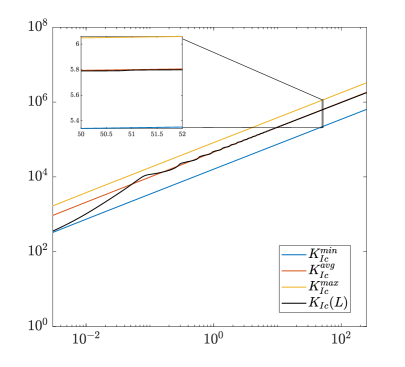
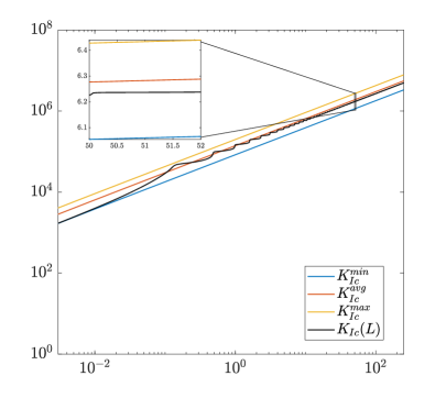
Figure B.6: The cumulative toughness energy expended fracturing the solid material $S$, (19), alongside the behaviour for the case of homogeneous toughness with distributions: maximum toughness $K_{Ic}(L)\equiv K_{Ic}^{max}$, minimum toughness $K_{Ic}(L)\equiv K_{Ic}^{min}$, and the (arithmetic) average toughness $K_{Ic}(L)\equiv K_{Ic}^{avg}$. We consider toughness distributions (a), (b) $\delta_{max}=1$, $\delta_{min}=0.1$, (c), (d) $\delta_{max}=10$, $\delta_{min}=1$, (e), (f) $\delta_{max}=100$, $\delta_{min}=10$, in the (a), (c), (e) sinusoidal, (b), (d), (f) step-wise, cases.

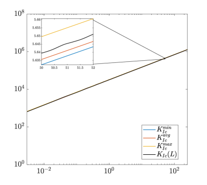
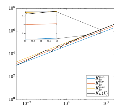
Figure B.7: The cumulative elastic energy $U$ stored within the solid material, (19), alongside the behaviour for the case of homogeneous toughness with distributions: maximum toughness $K_{Ic}(L)\equiv K_{Ic}^{max}$, minimum toughness $K_{Ic}(L)\equiv K_{Ic}^{min}$, and the (arithmetic) average toughness $K_{Ic}(L)\equiv K_{Ic}^{avg}$. We consider toughness distributions (a), (b) $\delta_{max}=1$, $\delta_{min}=0.1$, (c), (d) $\delta_{max}=10$, $\delta_{min}=1$, (e), (f) $\delta_{max}=100$, $\delta_{min}=10$, in the (a), (c), (e) sinusoidal, (b), (d), (f) step-wise, cases.

The acceleration of the fluid, discussed in the main text in Sect. 4, is provided in Fig. B.8. The corresponding figures for the fluid velocity are given in the main text as Fig. 11. Note that there is a high level of error for the fluid acceleration at late-time, due to the disproportionate impact of the local error for the fluid velocity $v$ on computations of this parameter (see e.g. the local error in Fig. LABEL:Fig_Energy_Balance_supp). The general trends however are accurately displayed.

It is clear that there is an exceptionally high peak acceleration, which occurs when transitioning between different rock layers. The maximum acceleration is strongly dependent on the toughness distribution, being order $10^{5}$m/s² for the step-wise distribution in the toughness-toughness case, but of order $10^{1}$m/s² for the sinusoidal distribution in the intermediate-viscosity case. Note also that the peak acceleration decreases as the crack propagates for the intermediate-viscosity regime, but remains almost constant for the toughness-toughness case (over the length-scale considered here).

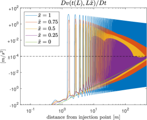
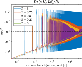
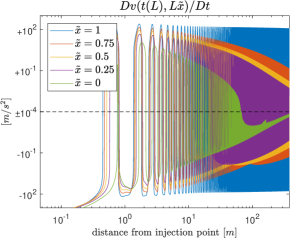
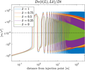
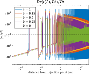
Figure B.8: Acceleration of the fluid particles inside the fracture for those 3 cases and 2 different toughness distributions in KGD model. (a), (b) $\delta_{max}=1$, $\delta_{min}=0.1$, (c), (d) $\delta_{max}=10$, $\delta_{min}=1$, (e), (f) $\delta_{max}=100$, $\delta_{min}=10$.

References

- [Bunger, 2013] Bunger, A. (2013). Analysis of the power input needed to propagate multiple hydraulic fractures. International Journal of Solids and Structures, 50(10):1538–1549.
- [Chen et al., 2024] Chen, R., Xu, W., Chen, Y., Nagel, T., Chen, C., Hu, Y., Li, J., and Zhuang, D. (2024). Influence of heterogeneity on dissolved co2 migration in a fractured reservoir. Environmental Earth Sciences, 83.
- [Da Fies, 2020] Da Fies, G. (2020). Efective time-space adaptive algorithm for hydraulic fracturing. PhD thesis, Aberystwth University, Aberystwyth.
- [Da Fies et al., 2021] Da Fies, G., Dutko, M., and Mishuris, G. (2021). Remarks on Dealing With Toughness Heterogeneity in Modelling of Hydraulic Fracture. volume All Days of U.S. Rock Mechanics/Geomechanics Symposium. ARMA-2021-2010.
- [Da Fies et al., 2023] Da Fies, G., Dutko, M., and Peck, D. (2023). Averaging-Based Approach to Toughness Homogenisation for Radial Hydraulic Fracture, pages 69–103. Springer International Publishing, Cham.
- [Da Fies et al., 2022] Da Fies, G., Peck, D., Dutko, M., and Mishuris, G. (2022). A temporal averaging–based approach to toughness homogenisation in heterogeneous material. Mathematics and Mechanics of Solids. (Accepted), eprint: https://doi.org/10.1177/10812865221117553.
- [Detournay and Peirce, 2014] Detournay, E. and Peirce, A. (2014). On the moving boundary conditions for a hydraulic fracture. International Journal of Engineering Science, 84:147–155.
- [Dontsov and Suarez-Rivera, 2021] Dontsov, E. and Suarez-Rivera, R. (2021). Representation of high resolution rock properties on a coarser grid for hydraulic fracture modeling. Journal of Petroleum Science and Engineering, 198:108144.
- [Garagash et al., 2011] Garagash, D., Detournay, E., and Adachi, J. (2011). Multiscale tip asymptotics in hydraulic fracture with leak-off. Journal of Fluid Mechanics, 669:260–297.
- [Geertsma and de Klerk, 1969] Geertsma, J. and de Klerk, F. (1969). A rapid method of predicting width and extent of hydraulically induced fractures. Journal of Petroleum Technology, 21 (12):1571–1581, SPE–2458–PA.
- [Kachanov and Sevostianov, 2018] Kachanov, M. and Sevostianov, I. (2018). Micromechanics of Materials, with Applications. Solid Mechanics and Its Applications. Springer, Cham.
- [Khristianovic Zheltov, 1955] Khristianovic Zheltov, A. (1955). Formation of vertical fractures by means of highly viscous liquid. In Proceedings of the fourth world petroleum congress, pages 579–586, Rome.
- [Lecampion et al., 2017] Lecampion, B., Desroches, J., Jeffrey, R. G., and Bunger, A. P. (2017). Experiments versus theory for the initiation and propagation of radial hydraulic fractures in low-permeability materials. Journal of Geophysical Research: Solid Earth, 122(2):1239–1263.
- [Lecampion and Detournay, 2007] Lecampion, B. and Detournay, E. (2007). An implicit algorithm for the propagation of a hydraulic fracture with a fluid lag. Computer Methods in Applied Mechanics and Engineering, 196(49):4863–4880.
- [Li et al., 2024] Li, K., Qi, C., Wang, M., Li, J., and Chen, H. (2024). Research on the influence of rock fracture toughness of layered formations on the hydraulic fracture propagation at the initial stage. Geohazard Mechanics, 2(2):121–130.
- [Li et al., 2020] Li, M., Guo, P., Stolle, D. F., Liang, L., and Shi, Y. (2020). Modeling hydraulic fracture in heterogeneous rock materials using permeability-based hydraulic fracture model. Underground Space, 5(2):167–183.
- [Linkov, 2011] Linkov, A. (2011). Speed equation and its application for solving ill-posed problems of hydraulic fracturing. Doklady Physics, 56 (8):436–438.
- [Linkov, 2012] Linkov, A. (2012). On efficient simulation of hydraulic fracturing in terms of particle velocity. International Journal of Engineering Science, 52:77–88.
- [Möri and Lecampion, 2021] Möri, A. and Lecampion, B. (2021). Arrest of a radial hydraulic fracture upon shut-in of the injection. International Journal of Solids and Structures, 219-220:151–165.
- [Möri et al., 2024] Möri, A., Peruzzo, C., Garagash, D., and Lecampion, B. (2024). How stress barriers and fracture toughness heterogeneities arrest buoyant hydraulic fractures. Rock Mechanics and Rock Engineering.
- [Oyedokun and Schubert, 2017] Oyedokun, O. and Schubert, J. (2017). A quick and energy consistent analytical method for predicting hydraulic fracture propagation through heterogeneous layered media and formations with natural fractures: The use of an effective fracture toughness. Journal of Natural Gas Science and Engineering, 44:351–364.
- [Peck et al., 2018] Peck, D., Wróbel, M., Perkowska, M., and Mishuris, G. (2018). Fluid velocity based simulation of hydraulic fracture: a penny shaped model—part i: the numerical algorithm. Meccanica, 53:3615 – 3635.
- [Perkowska et al., 2015] Perkowska, M., Wrobel, M., and Mishuris, G. (2015). Universal hydrofracturing algorithm for shear-thinning fluids: particle velocity based simulation. Computers and Geotechnics, 71:310–377.
- [Peruzzo, 2023] Peruzzo, C. (2023). Three-dimensional hydraulic fracture propagation in homogeneous and heterogeneous media. PhD thesis, EPFL, Lausanne.
- [Peruzzo et al., 2021] Peruzzo, C., Capron, J., and Lecampion, B. (2021). The breakthrough time of a hydraulic fracture contained between two tough layers. 19th Swiss Geoscience Meeting.
- [Peruzzo and Lecampion, 2024] Peruzzo, C. and Lecampion, B. (2024). How contained hydraulic fractures emerge from layers of alternating fracture toughness. 85th EAGE Annual Conference & Exhibition, 2024(1):1–5.
- [Peruzzo et al., 2024] Peruzzo, C., Möri, A., and Lecampion, B. (2024). The energy balance of a hydraulic fracture at depth. ArXiv Preprint, arXiv:2407.05785.
- [Ponson, 2023] Ponson, L. (2023). Fracture Mechanics of Heterogeneous Materials: Effective Toughness and Fluctuations, pages 207–254. Springer International Publishing, Cham.
- [Rueda et al., 2023] Rueda, C., Mejía, C., Paullo, L., Roehl, D., Rossi, D., and Henriques, F. (2023). 3D Hydraulic Fracture Propagation in a Heterogeneous Rock Formation Using a Mesh Transition Technique. U.S. Rock Mechanics/Geomechanics Symposium, All Days:ARMA–2023–0516.
- [Sarmadi et al., 2024] Sarmadi, N., Harrison, M., Nezhad, M. M., and Fisher, Q. J. (2024). Hydraulic fracture propagation in layered heterogeneous rocks with spatially non-gaussian random hydromechanical features. Rock Mechanics and Rock Engineering.
- [Savitski and Detournay, 2002] Savitski, A. and Detournay, E. (2002). Propagation of a penny-shaped fluid-driven fracture in an impermeable rock: asymptotic solutions. International Journal of Solids and Structures, 39:6311–6337.
- [Shi et al., 2023] Shi, X., Qin, Y., Gao, Q., Liu, S., Xu, H., and Yu, T. (2023). Experimental study on hydraulic fracture propagation in heterogeneous glutenite rock. Geoenergy Science and Engineering, 225:211673.
- [Stanchits et al., 2015] Stanchits, S., Burghardt, J., and Surdi, A. (2015). Hydraulic fracturing of heterogeneous rock monitored by acoustic emission. Rock Mechanics and Rock Engineering, 48:2513–2527.
- [Wang et al., 2024] Wang, Q., Yu, H., Xu, W., Huang, H., Li, F., and Wu, H. (2024). How does the heterogeneous interface influence hydraulic fracturing? International Journal of Engineering Science, 195:104000.
- [Wrobel and Mishuris, 2015] Wrobel, M. and Mishuris, G. (2015). Hydraulic fracture revisited: Particle velocity based simulation. International Journal of Engineering Science, 94:23–58.
- [Zeng and Wei, 2017] Zeng, X. and Wei, Y. (2017). Crack deflection in brittle media with heterogeneous interfaces and its application in shale fracking. Journal of the Mechanics and Physics of Solids, 101:235–249.
- [Zhong et al., 2024] Zhong, Y., Yu, H., Wang, Q., Chen, X., Ke, X., Huang, H., and Wu, H. (2024). Hydraulic fracturing in layered heterogeneous shale: The interaction between adjacent weak interfaces. Engineering Fracture Mechanics, 303:110115.