Controllable single-photon wave packet scattering in two-dimensional waveguide by a giant atom

Abstract

Nonlocal interactions between photonic waveguide and giant atoms have attracted extensive attentions. Researchers have studied how to optimize and control quantum states via giant atoms. We here study the dynamical scattering of a single-photon wave packet by a giant atom coupled to a two-dimensional photonic waveguide via multiple spatial points. We show that arbitrary target scattering single-photon wave packets can be generated by adjusting the coupling strength between the giant atom and different lattice sites of the waveguide. Furthermore, the dynamical scattering of the wave packets enables us to study the propagating properties of the target scattering wave packets and observe the excitation of giant atoms. Our study provides alternative way for photon state control based on giant atoms.

I introduction

Single-photon sources have important applications in quantum optics, quantum communication Couteau ; Luo , quantum metrology Eisaman ; Chunnilall , and quantum computation Maring . The best-performing single-photon source is based on the conditional detection for correlated photon pairs generated by spontaneous parametric down-conversion process DP . Single photons source can also be obtained via linear optics Darquie , spontaneous emission of quantum emitters two-level1 ; two-level2 ; two-level3 ; two-level4 and other approaches Hofmann ; Yuan . In practice, the single-photon source produces a light pulse with no more than one photon and is characterized by the second-order correlation function Senellart ; Zhai . A single-photon pulse is usually described by a single-photon wave packet state, which is a superposition of single-photon Fock states of infinite plane wave modes. To enhance the collection efficiency and the spontaneous emission rate of single-photons, the quantum emitter for single-photon sources is usually coupled to one-dimensional waveguides Zumofen ; Chang ; YChen or single-mode resonators Peng-NC . Moreover, to realize quantum information transfer via single-photons, arbitrarily controllable single-photon wave packets are highly desired Cai ; Srivathsan ; Tian . For example, specifically temporal shaped single-photon wave packets can be used for optical amplifiers Rephaeli2 ; Linares ; FWSun , deterministic quantum state transfers Cirac , and implementation of quantum logic gates Heuck .

Photon scattering by atoms or artificial atoms has emerged as one of powerful and straightforward quantum optical tools for manipulating the single-photon wave packets in the waveguide POGuimond ; Shi ; Shen ; Shi2 ; Xu ; Zheng ; Zhou ; Nie . However, in these studies POGuimond ; Shi ; Shen ; Shi2 ; Xu ; Zheng ; Zhou ; Nie , the atoms are considered as point particles and are assumed to be coupled to the waveguide via a point due to its negligible size compared to the wavelength of the modes in waveguide. Recently, in a seminal work, the superconducting qubits Gu-PR , acting as giant artificial atoms, were designed to interact with surface acoustic waves via multiple coupling points Andersson . From then on, the interaction between superconducting giant atoms and surface acoustic wave resonators was extensively studied SAW1 ; SAW2 ; SAW3 ; SAW4 ; SAW5 ; Xin2 ; Kannan ; xin2 , and the studies on giant atoms are also extended to cold atom systems GonzalezTudela and ferromagnetic spin systems ZQWang . Various new phenomena, e.g., retardation effect Cheng , frequency-dependent radiative decay rate Kockum , nonexponential decay Andersson2 ; Guo , and decoherence-free interaction Kockum2 , were found in the systems of giant atoms. Moreover, single-photon scattering has also been studied in a system of one-dimensional waveguide coupled to giant atoms via multiple points Chen ; Peng ; NLiu ; WZhao .

Two-dimensional waveguide or coupled-cavity waveguide systems can be used to simulate quantum phase transitions of light Greentree , realize quantum walks of correlated photons TD1 ; Jiao , photosynthetic energy transport Mohseni . The theoretical study shows that the relaxing of the giant atom can be avoided when the giant atom interacts with an environment of two-dimensional coupled-cavity waveguides Ingelsten . Moreover, coherent interaction between a quantum emitter and the edge states in two-dimensional optical topological insulators has been studied QE-T1 . Topological multimode waveguide QED with two-dimensional topological photonic system coupled to a quantum emitter has also been demonstrated QE-T2 . Furthermore, it has also been shown that the single-photon scattered by many atoms, interacting with a system of two-dimensional coupled-cavity waveguides, can exhibit collective effect  DZXu .

Stimulated by previous studies on single-photon scattering by an atom in one-dimensional waveguide or many atoms in two-dimensional photonic wavguides, we here study single-photon scattering by a giant atom coupled to two-dimensional photonic waveguides via multiple discrete points. We first show the dispersion effect on the size of the propagating wave packet and show how a stable wave packet can be obtained. Then we study the dynamical scattering of the single-photon wave packets by both the small and giant atoms via scattering matrix. By adjusting the coupling strengths of different coupling points between two-dimensional photonic wavguides and the giant atom, we find that the photon distribution of the target scattered single-photon wavepacket can be optimized. In addition, we also explore the propagating properties of the incident and target scattering wave packets via the propagating fidelity and study the excitation of giant atoms by single-photon wave packet. Finally, we compare the numerical results with analytical ones and show the effectiveness of our analytical studies.

The paper is organized as follows. In Sec. II, we describe the theoretical Hamiltonian model and derive a formula of the scattering matrix. In Sec. III, we introduce a theory to produce the desired incident single-photon wave packet in the two-dimensional photonic waveguide. The dispersion effect on the propagation of the single-photon wave packet is also studied. In Sec. IV, we use the scattering matrix to study the dynamical scattering of single-photon wave packet by a small atom. In Sec. V, we derive an optimization function and study controllable single-photon scattering based on the giant atom. In Sec. VI, we summarize our results and analyze the feasibility of the experiment.

II Theoretical Model and Scattering Matrix

II.1 Theoretical Model and Hamiltonian

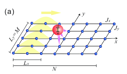
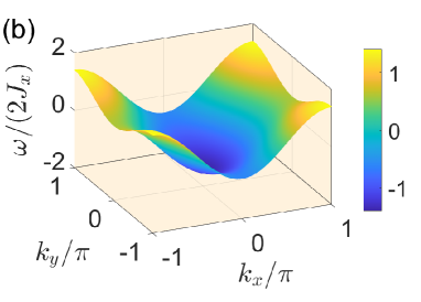
Figure 1: (a) Schematic diagram for the 2D photonic waveguide coupled to a giant atom. (b) The energy spectrum $\omega(\vec{k})$ of the 2D photonic waveguide. The parameters are set as: $\omega_{l}=0$, $J_{y}/(2J_{x})=0.2$.

As schematically shown in Fig. 1(a), we consider that a two-level giant atom, with the transition frequency $\omega_{a}$ between the ground state $|g\rangle$ and excited state $|e\rangle$, is coupled to a two-dimensional (2D) photonic waveguide via multiple spatial points. The Hamiltonian of the whole system can be written as

$$H=H_{0}+H_{{\rm G,I}}.$$ (1)

Where the free Hamiltonian $H_{0}$ of the 2D photonic waveguide and the giant atom is given by

$$H_{0}=H_{0}^{\prime}+\omega_{a}|e\rangle\langle e|,$$ (2)

with the free Hamiltonian $H^{\prime}_{0}$ of the 2D photonic waveguide

$$\begin{split}H_{0}^{\prime}&=\sum_{n,m}\left\{\omega_{l}a_{n,m}^{{\dagger}}a_{n,m}\right.-(J_{x}a_{n,m}^{{\dagger}}a_{n+1,m}\\ &+\left.J_{y}a_{n,m}^{{\dagger}}a_{n,m+1}+{\rm H.c})\right\},\end{split}$$ (3)

hereafter, we assume $\hbar=1$. $a_{n,m}$ and $a_{n,m}^{{\dagger}}$ are the annihilation and creation operators of the photonic mode on the lattice site $(n,m)$, respectively. The integer numbers $n$ and $m$ denote the discrete values in $x$-direction and $y$-direction, respectively. We also assume that all photonic modes have the same frequency $\omega_{l}$. Moreover, we assume that there are only the nearest-neighbor hopping interaction stremgths between different photonic modes. The parameters $J_{y}$ and $J_{x}$ denote the hopping strengths along $y$-axis and $x$-axis, respectively. $\sigma_{+}=|e\rangle\langle g|$ ($\sigma_{-}=|g\rangle\langle e|$) is the raising (lowering) operator of the two-level giant atom. The interaction Hamiltonian $H_{{\rm G,I}}$ between the giant atom and the photonic waveguide via multiple coupling points is given as

$$H_{{\rm G,I}}=\sum_{m_{1}=-M_{1}}^{M_{1}}\sum_{n_{1}=-N_{1}}^{N_{1}}\frac{g}{\Lambda}\left\{\lambda_{n_{1},m_{1}}a_{n_{1},m_{1}}\sigma^{+}+{\rm H.c}\right\}.$$

(4)

The summation is taken for all coupling points $(n_{1},m_{1})$. The parameter $g\lambda_{n_{1},m_{1}}/\Lambda$ represents the interaction between the giant atom and the photonic mode at a specific lattice site $(n_{1},m_{1})$ and $\Lambda=\sum_{n_{1},m_{1}}|\lambda_{n_{1},m_{1}}|$ is the normalization constant to ensure that the summation of all coupling strengths is equal to $g$. For convenience and without loss of generality, we assume that the site $(0,0)$ is the center of all coupling sites and the total number of the coupling points is $(2N_{1}+1)(2M_{1}+1)$.

Let us now apply the Fourier transform $a_{n,m}=\sum_{k_{x},k_{y}}a_{k_{x},k_{y}}e^{ik_{x}n+ik_{y}m}/\sqrt{MN}$ to the free Hamiltonian $H_{0}^{\prime}$ of the photonic waveguide under the periodical boundary condition with the total lattice numbers $N$ and $M$ in the $x$-axis and $y$-axis, and then the Hamiltonian $H_{0}^{\prime}$ in Eq. (3) is expressed as

$$H_{0}^{\prime}(\vec{k})=\sum_{k_{x},k_{y}}\omega(\vec{k})a_{k_{x},k_{y}}^{{\dagger}}a_{k_{x},k_{y}},$$ (5)

in the momentum space with

$$\omega(\vec{k})\equiv\omega(k_{x},k_{y})=\omega_{l}-2J_{x}\cos(k_{x})-2J_{y}\cos(k_{y}),$$ (6)

which has a cosine-type nonlinear structure. Here, the wavenumbers $k_{x}$ and $k_{y}$ are defined as $k_{x}\in\{-\pi,-\pi(N-1)/N,\cdots,0,\cdots,\pi(N-1)/N,\pi\}$ and $k_{y}\in\{-\pi,-\pi(M-1)/M,\cdots,0,\cdots,\pi(M-1)/M,\pi\}$. Equation (6) clearly shows that the energy spectrum $\omega(\vec{k})$ is in the range $[\omega_{l}-2J_{x}-2J_{y},\omega_{l}+2J_{x}+2J_{y}]$ and is an even function of $k_{x}$ and $k_{y}$. Thus, as shown in Fig. 1(b), $\omega(\vec{k})$ exhibits a symmetrical characteristics in both $k_{x}$ and $k_{y}$ directions.

In the momentum space under the Fourier transform $a_{n,m}=\sum_{k_{x},k_{y}}a_{k_{x},k_{y}}e^{ik_{x}n+ik_{y}m}/\sqrt{MN}$, the interaction Hamiltonian $H_{{\rm G,I}}$ in Eq. (4) can be rewritten as

$$H_{{\rm G,I}}(\vec{k})=\sum_{k_{x},k_{y}}\left\{G(\vec{k})a_{k_{x},k_{y}}\sigma^{+}+{\rm H.c}\right\},$$ (7)

with the coupling constant $G(\vec{k})$ between the giant atom and $\vec{k}=(k_{x},k_{y})$ mode photon

$$G(\vec{k})=\frac{g}{\Lambda}\sum_{n_{1},m_{1}}\lambda_{n_{1},m_{1}}e^{ik_{x}n_{1}+ik_{y}m_{1}},$$ (8)

which is derived from the summation of the coupling strengths of different coupling points in the position space and is characterized by the quantum interference.

II.2 Scattering Matrix

For the sake of completeness and convenience of following study, we now briefly summarize the theoretical description of the scattering process. In the scattering theory, the relation between final and initial states of the system can be expressed by the scattering matrix, which can be obtained via the scattering operator $S=U(t_{i},t_{f})$ from the initial time $t_{i}=-\infty$ to the final time $t_{f}=+\infty$ as POGuimond ; Taylor

$$S=1-2\pi i\delta(E_{f}-E_{i})T(E_{i}),$$ (9)

with

$$T(E_{i})=\sum_{n=0}^{\infty}H_{{\rm G,I}}\left(\frac{1}{E_{i}-H_{0}+i0^{+}}H_{{\rm G,I}}\right)^{n}.$$ (10)

Here, the subscripts $i$ and $f$ denote initial and final, respectively. In our study, the number of excitations is conserved since the Hamiltonian is derived in the rotating wave approximation. That is, the energy is conserved in the scattering process, which is guaranteed by $\delta$-function. For the case of a single photon scattering, $E_{i}$ and $E_{f}$ correspond to the energies of single-photons for the initial state $|\vec{k}_{i},g\rangle=|\vec{k}_{i}\rangle\otimes|g\rangle$ with the photon wave vector $\vec{k}_{i}$ and final state $|\vec{k}_{f},g\rangle=|\vec{k}_{f}\rangle\otimes|g\rangle$ with the photon wave vector $\vec{k}_{f}$, which satisfy equations $H_{0}|k_{i}\rangle=E_{i}|k_{i}\rangle$ and $H_{0}|k_{f}\rangle=E_{f}|k_{f}\rangle$, respectively. Here, the energies of the single-photons corresponding to the initial and final states are given as

$$E_{\alpha}=\omega(\vec{k}_{\alpha})=\omega_{l}-2J_{x}\cos(k_{\alpha,x})-2J_{y}\cos(k_{\alpha,y}),$$ (11)

for $\vec{k}_{\alpha}=(\vec{k}_{\alpha,x},\vec{k}_{\alpha,y})$ with $\alpha=i$ or $\alpha=f$. We note that the first term in Eq. (9) describes the free evolution of the single-photon packet, while the operator $T(E_{i})$ describes the scattering effect of the atoms on the single-photons. According to Ref. POGuimond , the matrix elements of the scattering operator in Eq. (9) can be written as (see details in Appendix A)

$$\langle g,\vec{k}_{f}|S|\vec{k}_{i},g\rangle = \langle\vec{k}_{f}|\vec{k}_{i}\rangle-\frac{i}{2\pi}\sum_{q}\frac{\delta(\vec{k}_{f}-\vec{q})}{|\nabla E_{f}|_{\vec{k}_{f}=\vec{q}}}\frac{G^{\ast}(\vec{k}_{f})G(\vec{k}_{i})}{E_{i}-\omega_{a}-\Sigma+i0^{+}}.$$ (12)

The parameter $\Sigma$ is the self-energy of the giant atom and is given by

$$\Sigma = \left\langle e,0\left|\frac{H_{G,I}}{E_{i}-H_{0}+i0^{+}}H_{G,I}\right|0,e\right\rangle$$

$$= \frac{1}{4\pi^{2}}\int dk_{x}dk_{y}\frac{|G(\vec{k})|^{2}}{E_{i}-\omega(\vec{k})+i0^{+}}.$$

The self-energy function is interpreted as the interaction energy between the giant atom and the photonic waveguide, whose imaginary part corresponds to the decay of an atomic excitation via photon and real part corresponds to the Lamb shift. From Eq. (12), we can obtain the scattering probability $s=|\langle g,\vec{k}_{i}|S|\vec{k}_{i},g\rangle|^{2}$ as

$$s=\left|1-\frac{i|G(\vec{k}_{i})|^{2}}{2\pi|\nabla E_{f}|_{\vec{k}_{f}=\vec{k}_{i}}(E_{i}-\omega_{a}-\Sigma+i0^{+})}\right|^{2}.$$ (14)

when we only consider $q=\vec{k}_{i}$.

III Dispersion effect on propagation of single-photon wave packet in 2D photonic waveguide

Our goal is to study the scattering of single-photon, which is described by a single-photon wave packet state. We know that a single-photon wave packet in continuous space can usually be expressed as YWang

$$|\psi(\vec{k})\rangle=\int d\vec{r}\phi(\vec{r})e^{i\vec{k}_{c}\cdot\vec{r}-i\vec{k}\cdot\vec{r}}a_{\vec{r}}^{{\dagger}}|0\rangle,$$ (15)

where $a_{\vec{r}}^{{\dagger}}$ is the creation operator at the position $\vec{r}$ and $\phi(\vec{r})$ is the spatial distribution function of the single-photon wave packet with $\int d\vec{r}|\phi(\vec{r})|^{2}=1$. $\vec{k}_{c}$ corresponds to the center wave vector. However, such a wave packet cannot stably propagate due to the dispersion even that the wave packet is not scattered by other subjects. Thus, before going to study the scattering of the single-photon wave packet, we first study the dispersion effect on the size of the wave packet when the wave packet propagates with a given group velocity. We also discuss how a stable wave packet can be obtained.

According to the dispersion relation of the wave vector and angular frequency in Eq. (6), the group velocity of photons in the $2$D photonic waveguide can be given as

$$\vec{v}=\nabla\omega(\vec{k})=(2J_{x}\sin(k_{x}),2J_{y}\sin(k_{y})).$$ (16)

Thus, if a single-photon wave packet propagates in the $2$D photonic waveguide with the group velocity $\vec{v}\sim(2J_{x},0)\equiv(v_{x}=2J_{x},v_{y}=0)$, then such wave packet is composed of modes $k_{x}\sim\pi/2$ and $k_{y}=0$, that is, the wave vector of this wave packet is $\vec{k}\sim(\pi/2,0)$. It is clear that there is no dispersion along $y$ direction when this wave packet propagates with the group velocity $\vec{v}\sim(2J_{x},0)$, but this wave packet has broadening along the $x$ direction with its propagation.

To better understand the dispersion effect on the propagation of the wave packet in $2$D photonic waveguide, we now assume that a single-photon wave packet is initially prepared to a state, for example,

$$|\psi_{0}\rangle=\sum_{m=-M}^{M}\alpha a_{n_{i},m}^{{\dagger}}|0,g\rangle,$$ (17)

where all sites of photonic excitations in the wave packet form a straight line with $n=n_{i}<0$ parallel to the $y$-axis, the size $L_{y}$ of the wave packet along $y$-axis is assumed to be $2M+1$, and the single-photon excitation at each lattice site $(n_{i},m)$ with $m=-M,\cdots,M$ has the same probability $|\alpha|^{2}$ with the normalization $(2M+1)|\alpha|^{2}=1$. That is, the size of the single-photon wave packet is initially a straight line with the length $2M+1$ along $y$ axis and locates in the left of the origin in the $x$ axis. The state $|0,g\rangle$ denotes that the giant atom is the ground state $|g\rangle$ and the $2$D photonic waveguide is in the vacuum state $|0\rangle$.

Let us assume that the single-photon wave packet in Eq. (17) freely propagates from the negative direction (the left side of the origin) to the positive direction (the right side of the origin) with the the group velocity $\vec{v}\sim(2J_{x},0)$. That is, we assume that the excited sites in $2$D photonic waveguide are far away from the giant atom or the $2$D photonic waveguide and the giant atom are decoupled from each other during the photon propagation, the giant atom has a negligibly small or no effect on the wave packet in the $2$D photonic waveguide. Thus, the time evolution of both $2$D photonic waveguide and the giant atom is governed by the free Hamiltonian in Eq. (2). Hereafter, the time evolution of the $2$D photonic waveguide is considered to be equivalent to the photon propagation.

It is clear that the wave packet has no broadening along $y$ direction due to $v_{y}=0$ when it propagates with the group velocity $\vec{v}\sim(2J_{x},0)$. That is, the size $2M+1$ of the $y$ direction for this wave packet is not changed with the time evolution. The size of the $x$ direction is increased with the time evolution. However, we find that the size of the propagating wave packet gradually tends stable. To obtain the the size of the stable wave packet, we now assume that the wave packet dynamically evolve with a time $T$ from initial state in Eq. (17) under the Hamiltonian $H_{0}$ given in Eq. (2), then the initial wave packet evolves to $|\psi_{1}\rangle=\exp(-iH_{0}T)|\psi_{0}\rangle$. Let us truncate a part in the position space from the wave packet $|\psi_{1}\rangle$ with the size $L_{x}\times L_{y}$ as schematically shown in Fig. 1(a), the center line $n=n_{i}$ along $y$ direction of the initial wave packet in Eq. (17) is now changed to $n=n_{i}+v_{x}T$ for the truncated wave packet, and the lattice site coordinate in $y$-axis of the truncated wave packet is not changed due to $v_{y}=0$ and still takes values $m=-M,\cdots,M$. The size $L_{x}$ is determined by the group velocity and is discussed below.

We normalize the truncated wave packet and use it as a new initial wave packet to evolve the same time $T$. Then we truncate another wave packet with the same size $L_{x}\times L_{y}$, but the the center line is now changed to $n=n_{i}+2v_{x}T$. We iterate such procedure many times. That is, the evolution time for each iteration is assumed to be $T$, the size of the truncated wave packet is $L_{x}\times L_{y}$, but the center line along $y$ direction for the truncated wave packet should add $v_{x}T$. The iteration is finished until the truncated wave packet with the size $L_{x}\times L_{y}$ has a stable fidelity discussed below in Eq. (19). We can assume that the formal solution of the truncated wave packet $|\psi_{i}(0)\rangle$ with the size $L_{x}\times L_{y}$ is written as

$$|\psi_{i}(0)\rangle=\sum_{m=-M}^{M}\sum_{n=-(L_{x}/2)+n_{f}}^{(L_{x}/2)+n_{f}}\beta_{n,m}e^{ik_{c,x}n+ik_{c,y}m}a_{n,m}^{{\dagger}}|0,g\rangle,$$

(18)

where the parameters $\beta_{n,m}$ satisfy the normalization condition $\sum_{m,n}|\beta_{n,m}|^{2}=1$, and are determined by $\alpha$ and the total time $T_{\rm total}$ of all iterations. The center line $n_{f}$ along $y$ direction for finally truncated wave packet should be $n_{f}=n_{i}+v_{x}T_{\rm total}$. In our calculation, we assume $n_{i}=-1047.5$ and $T=25/(2J_{x})$. We find that the size of $L_{x}$ is about $25$ with the given parameters when the wave packet reaches nearly stable with $n_{f}=-47.5$. The photon distribution $|\beta_{n,m}|^{2}$ of the wave packet in the position space is shown in Fig. 2(a). In Fig. 2(c), we plot the real and imaginary part of the initial wave packet $|\psi_{i}(0)\rangle$ in the momentum space. It confirms that photon distribution is confined to be around the central wave vector $\vec{k}_{c}$ with $k_{c,x}\sim\pi/2$ and $k_{c,y}=0$. We further study the time evolution of the wave packet with an evolution time $t$ when the initial state is expressed as $|\psi_{i}(0)\rangle$ in Eq. (18), then we find that the final state $|\psi_{f}(t)\rangle=\exp(-iH_{0}t)|\psi_{i}(0)\rangle$ with an evolution time $t=80/(2J_{x})$ exhibits localization in the position space and can propagate to the designated position with a group velocity $\vec{v}\sim(2J_{x},0)$ as show in Fig. 2(b). Its main photon distribution is concentrated in $m\in\{-M,\cdots,M\}$ and $n\in\{v_{x}t+n_{f}-(L_{x}/2),\cdots,v_{x}t+n_{f}+(L_{x}/2)\}$.

To describe the distortion degree of the wave packet during the propagation, we here define the propagating fidelity (${\rm PF}$) MichaelMurphy , which is inner product of the translational wave packet $D(t)|\psi_{i}(0)\rangle$ and the evolved wave packet $|\psi_{f}(t)\rangle$ with an evolution time $t$

$${\rm PF}=|\langle\psi_{f}(t)|D(t)|\psi_{i}(0)\rangle|^{2},$$ (19)

where

$$D=\sum_{m=-M}^{M}\sum_{n=-(L_{x}/2)+n_{f}}^{(L_{x}/2)+n_{f}}a^{{\dagger}}_{n+v_{x}t,m}a_{n,m}$$ (20)

is the translational operation on the initial wave packet with a translational distance $v_{x}t=2J_{x}t$. When ${\rm PF}=1$, we say that the wave packet perfectly propagates, otherwise when ${\rm PF}=0$, we say that the wave packet is completely distorted. In Fig. 2(d), we have exhibited the ${\rm PF}$ of the wave packet versus the time $t$. It shows that the ${\rm PF}$ decreases with the time evolution and oscillates periodically on local time scales. If the ${\rm PF}$ of the initial wave packet remains above 0.9 after propagating a distance equal to its own size of $L_{x}$ as shown by the red-dashed line in Fig. 2(d), then we consider the initial wave packet as an incident light source for studying the scattering of light. Below, we will study the scattering of the single-photon wave packet which has the group velocity $\vec{v}\sim(2J_{x},0)$ and is initially prepared to the state given in Eq. (18).

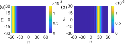
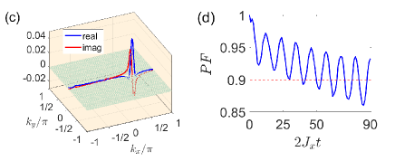
Figure 2: (a) The population distribution $|\langle\psi_{i}(0)|a^{{\dagger}}_{n,m}|0,g\rangle|^{2}$ at each lattice site $(n,m)$ for the wave packet state in Eq. (18). (b) The population distribution $|\langle\psi_{f}(t)|a^{{\dagger}}_{n,m}|0,g\rangle|^{2}$ at each lattice site $(n,m)$ for the wave packet $|\psi_{f}(t)\rangle$ with the evolution time $t=80/(2J_{x})$. Here, $m=-M,\cdots,M$ and $n=-N,\cdots,N$. (c) The real part ${\rm Re}(\langle\psi_{i}(0)|a^{{\dagger}}_{k_{x},k_{y}}|0,g\rangle)$ and imaginary part ${\rm Im}(\langle\psi_{i}(0)|a^{{\dagger}}_{k_{x},k_{y}}|0,g\rangle)$ in the moment space for the wave packet in Eq. (18). Here, $k_{x}=-\pi,-\pi(N-1)/N,\cdots,0,\cdots,\pi(N-1)/N,\pi$ and $k_{y}=-\pi,-\pi(M-1)/M,\cdots,0,\cdots,\pi(M-1)/M,\pi$. (d) The propagating fidelity PF of the initial wave packet versus the time $t$. The parameters are set $J_{y}/(2J_{x})=0.2$, $N=121$, $M=61$, $L_{x}=25$. $v_{x}t=2J_{x}t=80$ for (b).

IV Scattering Matrix and Scattering of Wave Packet by small atom

Let us now study the scattering of the single-photon wave packet by a small atom, which is consider as a point particle. That is, we assume that the small atom is coupled to the photonic lattice at the point $(0,0)$ and $\omega_{a}=\omega_{l}$. Thus, the coupling strength in Eq. (8) between the small atom and $2$D photonic waveguide in the momentum space is simplified to $G(\vec{k})=g$.

To study the scattering properties of the system, we assume that the atom is in the ground state $|g\rangle$ and the photonic waveguide is initially prepared to the wave packet state $|\psi_{i}(0)\rangle$ given in Eq. (18) and shown in Fig. 2(a). The single-photon wave packet propagates in the group velocity $\vec{v}\sim(2J_{x},0)$. With an evolution time $t$, the system is changed from the initial state $|\psi_{i}(0)\rangle$ to final state $|\psi_{s}(t)\rangle=\exp(-iHt)|\psi_{i}(0)\rangle$, where $H$ is the total Hamiltonian of the small atom and the photonic waveguide given in Eq. (1). As shown in Fig. 3(a), the photonic distribution $|\langle\psi_{s}(t)|a^{{\dagger}}_{n,m}|0,g\rangle|^{2}$ for the wave packet $|\psi_{s}(t)\rangle$ is plotted. It clearly shows that the atom has negligibly small effect on the part of the incident wave packet far from the atom during propagation, but the part of the incident wave packet close to the atom undergoes significant scattering. To clearly show the influence of the scatterer to the wave packet, we subtract the “background” as shown in Fig. 2(b) from Fig. 3(a), and calculate the photon distribution $|(\langle\psi_{s}(t)|-\langle\psi_{f}(t)|)a^{{\dagger}}_{n,m}|0,g\rangle|^{2}$ as shown in Fig. 3(b) with the state $|\psi_{f}(t)\rangle=\exp(-iH_{0}t)|\psi_{i}(0)\rangle$. It shows that the scattered photon distributes symmetrically around the small atom. The symmetry originates from the energy spectrum of the system as shown in Fig. 1(b). As shown in Fig. 3(c), we plot the photon distribution $|(\langle\psi_{s}(t)|-\langle\psi_{f}(t)|)a^{{\dagger}}_{k_{x},k_{y}}|0,g\rangle|^{2}$ in the momentum space. It shows that the photons distributed around the constant-energy surface of the system. In practice, the method of ”background” elimination can be attributed to the influence of the second term in the $S$-matrix in Eq. (12). Therefore, in Fig. 3(d), we plot the photon distribution $|\langle g,\vec{k}_{f}|S-1|\vec{k}_{i},g\rangle|^{2}$ in momentum space by using the analytic result in Eq. (12). The agreement of numerical and analytical results shows the rationality of our approach for dynamically simulating the scattering process.

We note that the scattering probability of the photons in one-dimensional systems can be significantly modulated by adjusting the frequency of the atoms and the coupling strength between the atoms and the waveguide Zhou ; Nie . However, in 2D systems, the photon scattered by a small atom evenly distributes around the constant-energy surface of the system. Therefore, we find that the distribution modulation of scattered photons by the coupling between the small atom and $2$D waveguide has the significant limitation. To overcome this limitation, we develop to the giant atom setup and design on demand scattering process by optimizing the coupling between the giant atom and the 2D photonic waveguide.

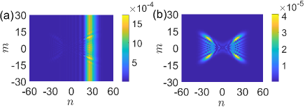
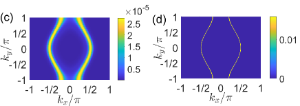
Figure 3: (a) and (b) The distribution diagrams of the scattering wave packets with $|\langle\psi_{s}(t)|a^{{\dagger}}_{n,m}|0,g\rangle|^{2}$ and without $|(\langle\psi_{s}(t)|-\langle\psi_{f}(t)|)a^{{\dagger}}_{n,m}|0,g\rangle|^{2}$ the “background” for the small atom, respectively. Here, $m=-M,\cdots,M$ and $n=-N,\cdots,N$ (c) The distribution diagram $|(\langle\psi_{s}(t)|-\langle\psi_{f}(t)|)a^{{\dagger}}_{k_{x},k_{y}}|0,g\rangle|^{2}$ of the scattering wave packet without the “background” in momentum space for the small atom. Here, $k_{x}\in\{-\pi,-\pi(N-1)/N,\cdots,0,\cdots,\pi(N-1)/N,\pi\}$ and $k_{y}\in\{-\pi,-\pi(M-1)/M,\cdots,0,\cdots,\pi(M-1)/M,\pi\}$. (d) The distribution of the photon scattering expression $|\langle g,\vec{k}_{f}|S-1|\vec{k}_{i},g\rangle|^{2}$ for the small atom. The parameters are set as: $n_{0}=m_{0}=0$, $J_{y}/(2J_{x})=0.2$, $N=121$, $M=61$, $L_{x}=25$, $g=2J_{x}$, $\omega_{l}=\omega_{a}=0$. $2J_{x}t=80$ for (a), (b) and (c).

V Controllable Scattering of Single-Photon Wave Packet by a Giant Atom

V.1 Optimization Function

We now turn to study the photon scattering by a giant atom. The nonlocal coupling between the giant atom and 2D waveguide via multiple spatial points results in nontrivial phase accumulations of the propagating field, which originates from the quantum interference between different coupling points. This quantum interference provides a possible way to optimally designs the photon scattering, which is different from that in the system of many atoms POGuimond ; DZXu . Here, we assume that all of the coupling points aline along the $y$-axis from the lattice site $(0,-M)$ to the site $(0,M)$, i.e., the giant atom-waveguide coupling points are symmetric with $y=0$. Then Eq. (8) can be simplified to

$$G(\vec{k})=\frac{2g}{\Lambda}\left\{\sum_{m_{1}=0}^{M_{1}}\lambda_{m_{1}}\cos(m_{1}k_{y})\right\}.$$ (21)

Here, we set $\lambda_{0,0}\rightarrow 2\lambda_{0}$ and $\lambda_{0,m_{1}}\equiv\lambda_{m_{1}}$ ($m_{1}=1,2,...,M_{1}$). We assume $\lambda_{m_{1}}=\lambda_{-m_{1}}$ when Eq. (21) is derived from Eq. (8). Thus, the parameter $2g\lambda_{0}/\Lambda$ is the coupling strength between the giant atom and the waveguide at the site $(0,0)$, and the parameter $g\lambda_{m_{1}}/\Lambda$ corresponds to the coupling strength between the giant atom and waveguide at the site $(0,\pm m_{1})$.

Table 1: The values of $\xi_{m_{1},m_{2}}$ with parameters $J_{y}/(2J_{x})=0.2$.

$\xi_{m_{1},m_{2}}$	$m_{2}=0$	$m_{2}=1$	$m_{2}=2$	$m_{2}=3$	$m_{2}=4$	$m_{2}=5$	$m_{2}=6$	$m_{2}=7$
$m_{1}=0$	-1.9985i	0.1470i	-0.0598i	0.0173i	-0.0061i	0.00207i	-0.00073i	0.000259
$m_{1}=1$		-0.6298i	0.08215i	-0.03295i	0.009679i	-0.0034i	0.001163i	-0.0004117i
$m_{1}=2$			-0.5208i	0.07454i	-0.0303i	0.0088i	-0.00309i	0.001082i
$m_{1}=3$				-0.6003i	0.0736i	-0.02996i	0.008663i	-0.003048i
$m_{1}=4$					-0.59997i	0.0735i	-0.02992i	0.008648i
$m_{1}=5$						-0.5994i	0.07351i	-0.02991i
$m_{1}=6$							-0.59993i	0.07351i
$m_{1}=7$								-0.59993i

We know that the single-photon wave packet is scattered by the giant atom to all directions with different momentums in the momentum space. However, if we can manipulate the coupling strengths between the giant atom and waveguide via the coupling points, then we can engineer the scattering photons to the expected state. In the following, we show how we can obtain an expected target scattering state, which is composed of several sets of momentum modes by well engineering the coupling constants of different coupling points. Hereafter, we refer to these momentums as expected momentums. Each set, e.g., the $j$th set of momentum modes in the target state, consists of four different momentum modes $(k_{{\rm xtar,j}},k_{{\rm ytar,j}}),~{}(-k_{{\rm xtar,j}},k_{{\rm ytar,j}}),~{}(k_{{\rm xtar,j}},-k_{{\rm ytar,j}}),$ $(-k_{{\rm xtar,j}},-k_{{\rm ytar,j}})$, which are symmetrical distribution in four quadrants of the $xy$-plane. The integer number $j$ labels the set of modes, $k_{{\rm xtar,j}}$ and $-k_{{\rm xtar,j}}$ ($k_{{\rm ytar,j}}$ and $-k_{{\rm ytar,j}}$) are assumed to be two centers for the $j$th set of modes in x (y) direction of the momentum space. They satisfy the relation $E_{i}-E(\vec{k}_{{\rm tar,j}})=0$.

To achieve the target scattering state with $j$ sets of momentum modes, we define an optimization function:

$$Q\equiv Q(k_{{\rm ytar,j}},k_{j},\lambda_{0},\lambda_{1}...\lambda_{M_{1}})=\frac{\Pi_{j}P_{j}}{O-\Sigma_{j}P_{j}},$$ (22)

with

$$P_{j}(k_{{\rm ytar,j}},k_{j},\{\lambda_{m_{1}}\})=\int_{-\pi}^{\pi}dk_{{\rm xf}}\int_{\Delta_{-}}^{\Delta_{+}}dk_{{\rm yf}}\left|S_{f,i}\right|^{2}$$ (23)

and

$$O(k_{{\rm ytar,j}},k_{j},\{\lambda_{m_{1}}\})=\int_{-\pi}^{\pi}dk_{{\rm xf}}\int_{0}^{\pi}dk_{{\rm yf}}\left|S_{f,i}\right|^{2}.$$ (24)

The function $P_{j}\equiv P_{j}(k_{{\rm ytar,j}},k_{j},\lambda_{0},...,\lambda_{M_{1}})\equiv P_{j}(k_{{\rm ytar,j}},k_{j},\{\lambda_{m_{1}}\})$ denotes the probability that the photon momentums of the scattering state are in the range $k_{x}\in(-\pi,\pi)$ and $k_{y}\in(\Delta_{-},\Delta_{+})$ with $\Delta_{\pm}=k_{{\rm ytar,j}}\pm k_{j}/2$ and $S_{f,i}=\langle g,\vec{k}_{f}|S-1|\vec{k}_{i},g\rangle$. Here, $k_{j}$ is the width of the $j$th set of the modes in $y$ direction. However, the function $O\equiv O(k_{{\rm ytar,j}},k_{j},\lambda_{0},...,\lambda_{M_{1}})\equiv O(k_{{\rm ytar,j}},k_{j},\{\lambda_{m_{1}}\})$ denotes the probability that the momentums of the scattering photons are in the range $k_{x}\in(-\pi,\pi)$ and $k_{y}\in(0,\pi)$. We note that we only consider the case of $0<k_{{\rm ytar,j}}<\pi$ due to the symmetric distribution of the target scattering state with the reflectional symmetric axis $y=0$. Then we have $k_{{\rm ytar,j}}-k_{j}/2\geq 0$ and $k_{{\rm ytar,j}}+k_{j}/2\leq\pi$.

In the optimization function $Q$, the continuous multiplication of $\{P_{j}\}$ guarantees that photons in the target scattering state have the expected momentum. The function $O-\Sigma_{j}P_{j}$ is the probability that photons in the target scattering state have no the expected momentum. To obtain the optimization function $Q$, we need to calculate the self-energy function $\Sigma$ given in Eq. (LABEL:self-energy) and the coupling strength in Eq. (21) which can be expanded as

$$|G(\vec{k})|^{2}=\frac{4|g|^{2}}{\Lambda^{2}}\left[\sum_{m_{1}=0}^{M_{1}}|\lambda_{m_{1}}|^{2}\cos^{2}(m_{1}k_{y})\right.$$ (25)

$$+\left.\sum_{m_{1}=0}^{M_{1}-1}\sum_{m_{2}=m_{1}+1}^{M_{1}}2{\rm Re}(\lambda^{*}_{m_{1}}\lambda_{m_{2}})\cos(m_{1}k_{y})\cos(m_{2}k_{y})\right].$$

with the normalized constant $\Lambda=\left(\sum_{m_{1}=0}^{m_{1}=M_{1}}2|\lambda_{m_{1}}|\right)^{2}$. If we define

$$\xi_{m_{1},m_{2}}=\frac{2J_{x}}{4\pi^{2}}\int dk_{x}dk_{y}\frac{\cos(m_{1}k_{y})\cos(m_{2}k_{y})}{\omega_{l}-2J_{y}-\omega(\vec{k})+i0^{+}},$$ (26)

then the self-energy function $\Sigma$ in Eq. (LABEL:self-energy) can be simplified to

$$\Sigma = \frac{4|g|^{2}}{2J_{x}\left(\sum_{m_{1}}|\lambda_{m_{1}}|\right)^{2}}\left\{\sum_{m_{1}=0}^{M_{1}}|\lambda_{m_{1}}|^{2}\xi_{m_{1},m_{1}}\right.$$ (27)

$$+ \left.\sum_{m_{1}=0}^{M_{1}-1}\sum_{m_{2}=m_{1}+1}^{M_{1}}2{\rm Re}(\lambda^{*}_{m_{1}}\lambda_{m_{2}})\xi_{m_{1},m_{2}}\right\}.$$

That is, once $\xi_{m_{1},m_{2}}$ and $\{\lambda_{m_{1}}\}$ are given, then we can obtain $\Sigma$. For example, in Table 1, a set of $\xi_{m_{1},m_{2}}$ is given for $15$ coupling points by numerical calculation when $J_{y}/(2J_{x})=0.2$. By optimizing coupling strengths $\{\lambda_{m_{1}}\}$, we can obtain the optimized function $Q$ and target scattering state.

To obtain the target scattering state with expected photon distributions, the optimization function $Q$ should be as large as possible by optimizing coupling strengths $\{\lambda_{m_{1}}\}$. Such maximization of the optimization function $Q$ can be converted to a convex optimization problem. Thus, we have to introduce optimization algorithms. For a relatively simple optimization function with few scattering modes, the gradient descent Ruder is sufficient to deal with it. However, when the optimization function is composed of many modes, the particle swarm optimization Kennedy is an optional effective optimization algorithm for obtaining the optimization function $Q$.

V.2 Controllable scattering of single-photon wave packet by a giant atom

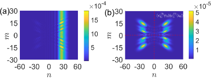
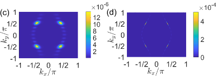
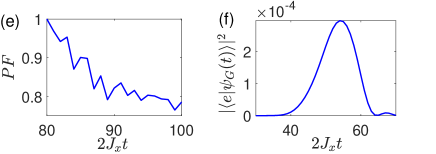
Figure 4: (a) and (b) The distribution diagrams of the scattering wave packets with $|\langle\psi_{G}(t)|a^{{\dagger}}_{n,m}|0,g\rangle|^{2}$ and without $|(\langle\psi_{G}(t)|-\langle\psi_{f}(t)|)a^{{\dagger}}_{n,m}|0,g\rangle|^{2}$ the “background” for the giant atoms, respectively. Here, $m=-M,\cdots,M$ and $n=-N,\cdots,N$. (c) The distribution diagram $|(\langle\psi_{G}(t)|-\langle\psi_{f}(t)|)a^{{\dagger}}_{k_{x},k_{y}}|0,g\rangle|^{2}$ of the scattering wave packet without the background in momentum space for the giant atom. (d) The distribution of the photon scattering expression $|\langle g,\vec{k}_{f}|S-1|\vec{k}_{i},g\rangle|^{2}$ for the giant atom. Here, $k_{x}\in\{-\pi,-\pi(N-1)/N,\cdots,0,\cdots,\pi(N-1)/N,\pi\}$ and $k_{y}\in\{-\pi,-\pi(M-1)/M,\cdots,0,\cdots,\pi(M-1)/M,\pi\}$. (e) The PF of the scattering wave packet versus the time $t$. (f) The excited state population $|\langle e,0|\psi_{G}(t)\rangle|^{2}$ of the giant atom versus the time $t$. The parameters are set as: $n_{0}=m_{0}=0$, $J_{y}/(2J_{x})=0.2$, $N=121$, $M=61$, $L_{x}=25$, $g/(2J_{x})=1$, $\omega_{l}=\omega_{a}=0$, $M_{1}=7$, $k_{ytar,1}=\pi/2$, $k_{1}=\pi/7$. $2\lambda_{0}:\lambda_{1}:\lambda_{2}:\lambda_{3}:\lambda_{4}:\lambda_{5}:\lambda_{6}:\lambda_{7}=1:-0.00088:-2.0547:-0.0476:2.1248:0.0026:-2.6811:-0.2156$. $2J_{x}t=80$ for (a), (b) and (c). $t_{0}=80/(2J_{x})$, $L^{\prime}_{x}=20$ and $L^{\prime}_{y}=18$ for (e).

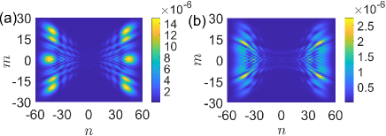
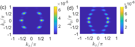
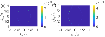
Figure 5: (a) and (b) The distribution diagrams $|(\langle\psi_{G}(t)|-\langle\psi_{f}(t)|)a^{{\dagger}}_{n,m}|0,g\rangle|^{2}$ of the scattering wave packets without the “background” for two different types of giant atoms. Here, $m=-M,\cdots,M$ and $n=-N,\cdots,N$. (c) and (d) The distribution diagrams $|(\langle\psi_{G}(t)|-\langle\psi_{f}(t)|)a^{{\dagger}}_{k_{x},k_{y}}|0,g\rangle|^{2}$ of the scattering wave packets without the “background” in momentum space for two different types of giant atoms. Here, $k_{x}\in\{-\pi,-\pi(N-1)/N,\cdots,0,\cdots,\pi(N-1)/N,\pi\}$ and $k_{y}\in\{-\pi,-\pi(M-1)/M,\cdots,0,\cdots,\pi(M-1)/M,\pi\}$. (e) and (f) The distributions of the photon scattering expression $|\langle g,\vec{k}_{f}|S-1|\vec{k}_{i},g\rangle|^{2}$ from two different types of giant atoms. The parameters are set as: $n_{0}=m_{0}=0$, $J_{y}/(2J_{x})=0.2$, $N=121$, $M=61$, $L_{x}=25$, $g/(2J_{x})=1$, $\omega_{l}=\omega_{a}=0$, $M_{1}=7$, $2J_{x}t=100$ for (a), (b), (c) and (d). $k_{ytar,1}=\pi/28$, $k_{ytar,2}=\pi/2$, $k_{1}=\pi/14$, $k_{2}=pi/7$, $2\lambda_{0}:\lambda_{1}:\lambda_{2}:\lambda_{3}:\lambda_{4}:\lambda_{5}:\lambda_{6}:\lambda_{7}=1:-1.4332:-3.2858:-1.3093:1.1984:-1.3141:-3.2387:-0.9584$ for (a), (c) and (e). $k_{ytar,1}=\pi/7$, $k_{ytar,2}=3\pi/7$, $k_{ytar,3}=5\pi/7$, $k_{ytar,4}=27\pi/28$, $k_{1}=k_{2}=k_{3}=\pi/7$, $k_{4}=pi/14$, $2\lambda_{0}:\lambda_{1}:\lambda_{2}:\lambda_{3}:\lambda_{4}:\lambda_{5}:\lambda_{6}:\lambda_{7}=1:0.3509:0.2903:-0.0347:0.00684:0.1582:-0.1743:-0.9628$ for (b), (d) and (f).

By using the optimization function $Q$ and the gradient descent algorithm, we can obtain a set of optimal coupling parameters $\{\lambda_{m_{1}}\}$ to achieve the target scattering states. For instance, we assume that the giant atom is coupled to the $2$D photonic waveguide through $15$ coupling points, the system is initially in the state given in Eq. (18), and the photons propagate with the group velocity $\vec{v}=(2J_{x},0)$. If we expect that the target scattering state has a stable configuration in the momentum space as shown in Fig. 4(c) after the single-photon wave packet is scattered by the giant atom with a time $t$, then we can use the optimization function $Q$ and the gradient descent algorithm to obtain the optimal coupling parameters, which satisfy the condition $2\lambda_{0}:\lambda_{1}:\lambda_{2}:\lambda_{3}:\lambda_{4}:\lambda_{5}:\lambda_{6}:\lambda_{7}=1:-0.00088:-2.0547:-0.0476:2.1248:0.0026:-2.6811:-0.2156$.

For above optimized coupling strengths, let us show the behavior of the target scattering state $|\psi_{G}(t)=\exp(-iHt)|\psi_{i}(0)\rangle$ with the scattering time $t$ in the position space, where $|\psi_{i}(0)\rangle$ is given in Eq. (18) and the total Hamiltonian $H$ is given in Eq. (1) for $15$ coupling points with above optimized coupling strengths. In the position space, the photon distribution $|\langle\psi_{G}(t)|a^{{\dagger}}_{n,m}|0,g\rangle|^{2}$ is plotted in Fig. 4(a). In Fig. 4(b), the photon distribution $|(\langle\psi_{G}(t)|-\langle\psi_{f}(t)|)a^{{\dagger}}_{n,m}|0,g\rangle|^{2}$ is plotted when we subtract the “background” state $|\psi_{f}(t)\rangle=\exp(-iH_{0}t)|\psi_{i}(0)\rangle$ with $H_{0}$ given in Eq. (2). Both Fig. 4(a) and Fig. 4(b) clearly show that the configuration of initial state $|\psi_{i}(0)\rangle$ in Eq. (18) shown in Fig. 2(a) is changed by the giant atom. We can also find that the target scattering single-photon wave packet in Fig. 4(c) composed of the set of the modes $\{(\arccos(J_{y}/J_{x}),\pi/2),(-\arccos(J_{y}/J_{x}),\pi/2)$, $(\arccos(J_{y}/J_{x}),-\pi/2),(-\arccos(J_{y}/J_{x}),-\pi/2)\}$. The group velocities $\vec{v}_{x}=2J_{x}$ and $\vec{v}_{y}=0$ of the incident wave packet are changed to $v_{x}=\pm 2\sqrt{1-(J_{y}/J_{x})^{2}}J_{x}$ and $v_{y}=\pm 2J_{y}$ after the wave packet is scattered by the giant atom. We note that the photon distribution in Fig. 4(c) is plotted by using $|(\langle\psi_{G}(t)|-\langle\psi_{f}(t)|)a^{{\dagger}}_{k_{x},k_{y}}|0,g\rangle|^{2}$ in the momentum space. We further plot $|\langle g,\vec{k}_{f}|S-1|\vec{k}_{i},g\rangle|^{2}$ in Fig. 4(d) by using above optimized coupling strengths. We find that Fig. 4(c) agrees well with Fig. 4(d).

To study the propagation of the target scattering single-photon wave packet, we can project the target scattering wave packet ($|\psi_{G}(t)\rangle-|\psi_{f}(t)\rangle$) in Fig. 4(b) to four subspaces with four states denoted as $|\psi_{G}^{(j)}(t)\rangle$ with $j=1,2,3,4$. These four states have up-down and left-right symmetries as shown by the red-dashed lines in Fig. 4(b). The symmetry makes sure that each state has the same photon propagating behavior. Therefore, we here focus on one state to study the propagating fidelity (${\rm PF}$) of the target scattering photons. For instance, if we consider the top-right state $|\psi_{G}^{(2)}(t)\rangle$ in Fig. 4(b), then the ${\rm PF}$ can be given as

$${\rm PF}=\frac{|\langle\psi_{G}^{(2)}(t)|D(t)|\psi_{G}^{(2)}(t_{0})\rangle|^{2}}{|\langle\psi_{G}^{(2)}(t_{0})|\psi_{G}^{(2)}(t_{0})\rangle|^{2}},$$ (28)

where

$$D(t)=\sum_{m=1}^{L_{y}^{\prime}}\sum_{n=1}^{L_{x}^{\prime}}a^{{\dagger}}_{n+v_{x}(t-t_{0}),m+v_{y}(t-t_{0})}a_{n,m}$$ (29)

being the translational operation of the initial scattering single-photon wave packet with the an integer translational distance $\vec{r}=(v_{x}(t-t_{0}),v_{y}(t-t_{0}))$ and $\vec{v}=(v_{x},v_{y})$ is the group velocity of the target scattering wave packet. $t_{0}$ is the artificially selected initial time of the target scattering wave packet and $L_{x}^{\prime}\times L_{y}^{\prime}$ is the size of the target scattering wave packet $|\psi_{G}^{(2)}(t)\rangle$. We find that the ${\rm PF}$ of the scattering photon is still close to 0.8 as shown in Fig. 4(e) after propagating a distance equal to its own size of $L^{\prime}_{x}$. This behavior originates from a compact distribution of the single-photon wave packet in momentum space, as shown in Fig. 4(c). Moreover, the dynamical evolutions of the wave packets provide us with a convenient way to observe the excitation of giant atom during the scattering process. In Fig. 4(f), we show the evolution of the excited state population $|\langle e,0|\psi_{G}(t)\rangle|^{2}$ of the giant atom. The asymmetry for the excitation of the giant atom in Fig. 4(f) result in an asymmetrical photon distribution of single-photon scattering wave packet in the position space as shown in Fig. 4(b).

Moreover, by implementing the particle swarm optimization to adjust the coupling strengths at different coupling points, the target scattering photon state with complex configuration can also be produced. For example, if we want to obtain the target scattering state, with photon distribution $|(\langle\psi_{G}(t)|-\langle\psi_{f}(t)|)a^{{\dagger}}_{n,m}|0,g\rangle|^{2}$ without “background” as shown in Fig. 5(a) in position space corresponding to the photon distribution $|(\langle\psi_{G}(t)|-\langle\psi_{f}(t)|)a^{{\dagger}}_{k_{x},k_{y}}|0,g\rangle|^{2}$ shown in Fig. 5(c) in the momentum space with multiple modes, then we can use the particle swarm optimization algorithm to obtain optimal coupling strengths, which satisfy the condition $2\lambda_{0}:\lambda_{1}:\lambda_{2}:\lambda_{3}:\lambda_{4}:\lambda_{5}:\lambda_{6}:\lambda_{7}=1:-1.4332:-3.2858:-1.3093:1.1984:-1.3141:-3.2387:-0.9584$. We also plot $|\langle g,\vec{k}_{f}|S-1|\vec{k}_{i},g\rangle|^{2}$ in Fig. 5(e) using optimized coupling strengths. Figure 5(e) agrees well with Fig. 5(c). If we want to obtain a target scattering state with photon distribution $|(\langle\psi_{G}(t)|-\langle\psi_{f}(t)|)a^{{\dagger}}_{n,m}|0,g\rangle|^{2}$ without “background” as shown in Fig. 5(b) in position space corresponding to the photon distribution $|(\langle\psi_{G}(t)|-\langle\psi_{f}(t)|)a^{{\dagger}}_{k_{x},k_{y}}|0,g\rangle|^{2}$ in momentum space as shown in Fig. 5(d), then we can use the particle swarm optimization algorithm to obtain another set of optimal coupling strengths, which satisfy the condition $2\lambda_{0}:\lambda_{1}:\lambda_{2}:\lambda_{3}:\lambda_{4}:\lambda_{5}:\lambda_{6}:\lambda_{7}=1:0.3509:0.2903:-0.0347:0.00684:0.1582:-0.1743:-0.9628$. We also plot $|\langle g,\vec{k}_{f}|S-1|\vec{k}_{i},g\rangle|^{2}$ in Fig. 5(f) using optimized coupling strengths. Figure 5(f) agrees well with Fig. 5(d). Thus, we conclude that the target scattering state can be obtained by optimizing the coupling strengths via the optimization function $Q$ in Eq. (22) and optimization algorithms.

We note that it is necessary to have a sufficient interaction time between the wave packet and the giant atom for realizing the scattering of single-photon scattering. It is clear that the self-energy function $\Sigma$ in Eq. (LABEL:self-energy) is purely imaginary number and corresponds to the system decay with the rate $\gamma=|\Sigma|$ determined by the coupling between the waveguide and the giant atom. Thus, to realize scattering, the interaction time $\tau=L_{x}/v_{x}$ between the incident wave packet and the atom should satisfy the condition $\tau\gg 1/\gamma$, where $1/\gamma$ is the lifetime of the atomic excited state. That is, the giant atom should be strongly coupled to the waveguide or the single-photon wave packet should have large enough width. In our numerical somulations, we assume $2J_{x}\tau=25$, $2J_{x}/\gamma\thickapprox 0.8334$ Fig. 3(d), $2J_{x}/\gamma\thickapprox 4.7461$ for Fig. 4(d), $2J_{x}/\gamma\thickapprox 8.3091$ for Fig. 5(e), $2J_{x}/\gamma\thickapprox 3.7397$ for Fig. 5(f). For these parameters, the atoms and the wave packets have the sufficient interaction time.

V.3 Transmission Probabilities

We emphasize that our study mainly focuses on the distributions of the scattering photons. However, traditional scattering problems primarily study the scattering or transmission probabilities Zhou ; Nie . Corresponding to Fig. 3 and Fig. 4(d), we can obtain transmission probabilities derived from Eq. (14) $T\thickapprox 0.7771$ and $T\thickapprox 0.9951$, respectively. However, corresponding to Figs. 5(e) and (f), the transmission probabilities are given by $T\thickapprox 0.9749$ and $T\thickapprox 0.9940$, respectively. That is, only a small portion of the photons is scattered, this is owing to the locality of the coupling patterns compared to the size of the incident wave packet. In Figs. 6(a) and (b), we plot the transmission probabilities $T$ versus the coupling strength $g$ and the detuning $\Delta$ for the small atom and giant atom, respectively. Here, $g$ is the coupling strength of the atom and $\Delta=\omega_{l}-\omega_{a}$. With these parameters, there is no the Lamb shift [${\rm Re}(\Sigma)=0$]. We observe a symmetric structure with the reflectional symmetric axis $\Delta-2J_{y}=0$ and the transmission probabilities have the minimum values on this axis, e.g., $T_{\rm min}=0.7523$ for Fig. 6(a) and $T_{\rm min}=0.9774$ for Fig. 6(b). When $\Delta-2J_{y}\neq 0$, the transmission probabilities are decay with the increase of $|g|$ and the transmission windows become wider as $|g|$ gets larger.

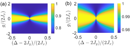
Figure 6: (a) and (b) The transmission probabilities $T$ versus the coupling strength $g$ and the detuning $\Delta$ for the small atom and giant atom, respectively. The parameters are set as: $n_{0}=m_{0}=0$, $J_{y}/(2J_{x})=0.2$. $M_{1}=7$ and $2\lambda_{0}:\lambda_{1}:\lambda_{2}:\lambda_{3}:\lambda_{4}:\lambda_{5}:\lambda_{6}:\lambda_{7}=1:-0.00088:-2.0547:-0.0476:2.1248:0.0026:-2.6811:-0.2156$ for (b).

VI Conclusion

In summary, we have studied the single-photon scattering in a 2D photonic waveguide coupled to a giant atom. We calculate the S-matrix of the system and propose an optimization function to control scattering photons. To simulate the scattering of single photons, we first study the dispersion effect on the size of the single-photon wave packet during the photon propagation. We particularly show that the size of a wave packet may reach nearly stable with the time evolution when the photon excitations of the initial wave packet aline along $y$-direction in the position space. We then consider such a wave packet with a stable size as the incident state and study the dynamical scattering of such wave packet by either a small atom or a giant atom. For the small atom, we find that the scattering photons evenly distribute around the constant energy surface of the system. However, for the giant atom, the scattering photon distribution can be tuned by optimizing the coupling strengths between the giant atom and different lattice sites of the $2$D photonic waveguide. We particularly show how to generate the arbitrary target scattering single-photon wave packet composed of the set of the symmetrical modes using the giant atom. Moreover, we also study the $\rm PF$ of the target scattering wave packets and calculate the excitation of giant atoms during the photon scattering process. Control of propagation and scattering for light fields in $2$D photonic waveguides plays a crucial role for the integrated on chip all-optical devices Altug ; Majumdar , thus our study for the control of the scattering photons by the giant atom may have a potential application in $2$D photonic devices.

With the current technoloy, our model may be implementable by using superconducting quantum circuits, in which the superconducting qubits and ${\rm LC}$ resonator arrays act as the giant atoms and the microwave photonic waveguides, respectively Gu-PR ; Roushan ; Hacohen-Gourgy ; Saxberg . The coupling strengths between the superconducting qubits and ${\rm LC}$ resonators can be tuned using various methods Goren . The decoherence time of the superconducting qubit circuits is about $100~{}\mu$s, while the energy scales of ${\rm LC}$ resonator arrays are typically in the range 100${\rm MHz}$-10${\rm GHz}$ Carroll ; Georgescu . Moreover, the synthetic frequency dimension has been recently proposed and extensively explored in a variety of physical systems LuqiYuan1 , e.g., in the system of the giant atoms coupled to the waveguide Du . Thus, the dynamics can be observed within the coherence time for our photon scattering proposal. We finally point out that our proposal for the dynamical scattering of wave packets can be applied to study the scattering problem in other systems composed of waveguides and atoms.

Appendix A Derivation of the matrix elements of scattering matrix

According to Ref. POGuimond , we can calculate the matrix elements of scattering matrix in Eq. (9) as

$$\langle g,\vec{k}_{f}|S|\vec{k}_{i},g\rangle = \langle\vec{k}_{f}|\vec{k}_{i}\rangle-2\pi i\delta(E_{f}-E_{i})\langle g,\vec{k}_{f}|\sum_{n=0}^{\infty}H_{\rm G,I}\left(\frac{1}{E_{i}-H_{0}+i0^{+}}H_{\rm G,I}\right)^{n}|\vec{k}_{i},g\rangle$$ (30)

$$= \langle\vec{k}_{f}|\vec{k}_{i}\rangle-2\pi i\delta(E_{f}-E_{i})\langle g,\vec{k}_{f}|H_{\rm G,I}\sum_{n=0}^{\infty}\left(\frac{1}{E_{i}-H_{0}+i0^{+}}H_{\rm G,I}\right)^{n}\frac{1}{E_{i}-H_{0}+i0^{+}}H_{\rm G,I}|\vec{k}_{i},g\rangle$$

$$= \langle\vec{k}_{f}|\vec{k}_{i}\rangle-2\pi i\delta(E_{f}-E_{i})\frac{G^{\ast}(\vec{k}_{f})G(\vec{k}_{i})}{E_{i}-\omega_{a}+i0^{+}}\langle e,0|\sum_{n=0}^{\infty}\left(\frac{1}{E_{i}-H_{0}+i0^{+}}H_{G,I}\right)^{n}|0,e\rangle$$

$$= \langle\vec{k}_{f}|\vec{k}_{i}\rangle-2\pi i\delta(E_{f}-E_{i})\frac{G^{\ast}(\vec{k}_{f})G(\vec{k}_{i})}{E_{i}-\omega_{a}+i0^{+}}\langle e,0|\sum_{n=0}^{\infty}\left[\frac{1}{E_{i}-\omega_{a}+i0^{+}}\left(\frac{H_{\rm G,I}}{E_{i}-H_{0}+i0^{+}}H_{\rm G,I}\right)\right]^{n}|0,e\rangle$$

$$= \langle\vec{k}_{f}|\vec{k}_{i}\rangle-\frac{i}{2\pi}\sum_{q}\frac{\delta(\vec{k}_{f}-\vec{q})}{|\nabla E_{f}|_{\vec{k}_{f}=\vec{q}}}\frac{G^{\ast}(\vec{k}_{f})G(\vec{k}_{i})}{E_{i}-\omega_{a}-\Sigma+i0^{+}}.$$

The summation of the first line in Eq. (12) can be rewritten to the second line by using the relation $\langle g,\vec{k}_{f}|H_{\rm G,I}|\vec{k}_{i},g\rangle=0$. We further insert the unit operator $|0,e\rangle\langle e,0|+\sum_{k}|k,g\rangle\langle g,k|$ into the summation of the second line, then we find that the contribution of the summation in the third line is only from the terms of even number $n$, all terms with the odd numbers are zero. Thus, we can further rewrite the summation of the third line to the fourth line by only considering the terms of the even number. In the last line, we also use the relation $\sum_{n=0}^{\infty}x^{n}=1/(1-x)$ and change the summation into the integral. From the fourth line to the fifth line, we use $\delta[\varphi(x)]=\sum_{i}\delta(x_{i})/|\varphi^{\prime}(x_{i})|$ such that $\delta(E_{f}-E_{i})$ for energy can be changed to $\delta(\vec{k}_{f}-\vec{q})$ for wavevector, where $q$ is root of the equation $E(\vec{k}_{f})-E(\vec{k}_{i})=0$ for variable $\vec{k}_{f}$ with the given initial wavevector $\vec{k}_{i}$ of the incident single-photon wavepacket.

References

- (1) C. Couteau, S. Barz, T. Durt, T. Gerrits, J. Huwer, R. Prevedel, J. Rarity, A. Shields, and G. Weihs, Applications of single photons to quantum communication and computing, Nat. Rev. Phys. 5, 326 (2023).
- (2) W. Luo, L. Cao, Y. Shi, L. Wan, H. Zhang, S. Li, G. Chen, Y. Li, S. Li, Y. Wang, S. Sun, M. F. Karim, H. Cai, L. C. Kwek, and A. Q. Liu, Recent progress in quantum photonic chips for quantum communication and internet, Light Sci. Appl. 12, 175 (2023).
- (3) M. D. Eisaman, J. Fan, A. Migdall, and S. V. Polyakov, Invited Review Article: Single-photon sources and detectors, Rev. Sci. Instrum. 82, 071101 (2011).
- (4) C. J. Chunnilall, I. P. Degiovanni, S. Kück, I. Müller, and A. G. Sinclair, Metrology of single-photon sources and detectors: a review, Opt. Eng. 53, 081910 (2014).
- (5) N. Maring, A. Fyrillas, M. Pont, E. Ivanov, P. Stepanov, N. Margaria, W. Hease, A. Pishchagin, A. Lemaitre, I. Sagnes, T. H. Au, S. Boissier, E. Bertasi, A. Baert, M. Valdivia, M. Billard, O. Acar, A. Brieussel, R. Mezher, S. C. Wein, A. Salavrakos, P. Sinnott, D. A. Fioretto, P. E. Emeriau, N. Belabas, S. Mansfield, P. Senellart, J. Senellart, and N. Somaschi, A versatile single-photon-based quantum computing platform, Nat. Photon. 79, 1 (2024).
- (6) D. C. Burnham and D. L. Weinberg, Observation of simultaneity in parametric production of optical photon pairs, Phys. Rev. Lett. 25, 84 (1970).
- (7) E. Knill, R. Laflamme, and G. J. Milburn, A scheme for efficient quantum computation with linear optics, Nature 409, 46 (2001).
- (8) H. J. Kimble, M. Dagenais and L. Mandel, Photon antibunching in resonance fluorescence, Phys. Rev. Lett. 39, 691 (1977).
- (9) F. Diedrich, and H. Walther, Nonclassical radiation of a single stored ion, Phys. Rev. Lett. 58, 203 (1987).
- (10) T. Basche, W. E. Moerner, M. Orrit, and H. Talon, Photon antibunching in the fluorescence of a single dye molecule trapped in a solid, Phys. Rev. Lett. 69, 1516 (1992).
- (11) Z. Yuan, B. E. Kardynal, R. M. Stevenson, A. J. Shields, C. J. Lobo, K. Cooper, N. S. Beattie, D. A. Ritchie, M. Pepper, Electrically Driven Single-Photon Source, Science 295, 102 (2002).
- (12) J. Hofmann, M. Krug, N. Ortegel, L. Gérard, M. Weber, W. Rosenfeld, and H. Weinfurter, Heralded entanglement between widely separated atoms, Science 337, 72 (2012).
- (13) C. H. Yuan, L. Q. Chen, Z. Y. Ou, and W. Zhang, Generation of frequency-multiplexed entangled single photons assisted by entanglement, Phys. Rev. A 83, 054302 (2011).
- (14) P. Senellart, G. Solomon, and A. White, High-performance semiconductor quantum-dot single-photon sources, Nat. Nanotechnol. 12, 1026 (2017).
- (15) L. Zhai, and A. Javadi, Harmonizing single photons with a laser pulse, Nat. Nanotechnol. 17, 436 (2022).
- (16) G. Zumofen, N. M. Mojarad, V. Sandoghdar, and M. Agio, Perfect Reflection of Light by an Oscillating Dipole, Phys. Rev. Lett. 101, 180404 (2007).
- (17) D. E. Chang, A. S. Sorensen, P. R. Hemmer, and M. D. Lukin, A single-photon transistor using nanoscale surface plasmons, Nat. Phys. 3 807 (2007).
- (18) Y. Chen, M. Wubs, J. Mørk, and A F. Koenderink, Coherent single-photon absorption by single emitters coupled to one-dimensional nanophotonic waveguides, New J. Phys. 13 103010 (2011).
- (19) Z. Peng, S. De Graaf, J. Tsai, and O. Astafiev, Tuneable on-demand single-photon source in the microwave range, Nat. Commun. 7, 12588 (2016).
- (20) M. Cai, Y. Lu, Z. Y. Ou, and W. Zhang, Optimizing single-photon generation and storage with machine learning, Phys. Rev. A 104, 053707 (2021).
- (21) B. Srivathsan, G. K. Gulati, A. Cere, B. Chng, and C. Kurtsiefer, Reversing the Temporal Envelope of a Heralded Single Photon using a Cavity, Phys. Rev. Lett. 113, 163601 (2014).
- (22) Z. Tian, Q. Liu, Y. Tian, and Y. Gu,Wavepacket interference of two photons: from temporal entanglement to wavepacket shaping, arXiv:2403.04432v1 (2024).
- (23) E. Rephaeli and S. Fan, Stimulated Emission from a Single Excited Atom in a Waveguide, Phys. Rev. Lett. 108, 143602 (2012).
- (24) A. Lamas-Linares, C. Simon, J. C. Howell, and D. Bouwmeester, Experimental Quantum Cloning of Single Photons, Science 296, 712 (2002).
- (25) F. W. Sun, B. H. Liu, Y. X. Gong, Y. F. Huang, Z. Y. Ou, and G. C. Guo, Stimulated Emission as a Result of Multiphoton Interference, Phys. Rev. Lett. 99, 043601 (2007).
- (26) J. I. Cirac, P. Zoller, H. J. Kimble, and H. Mabuchi, Quantum State Transfer and Entanglement Distribution among Distant Nodes in a Quantum Network, Phys. Rev. Lett. 78, 3221 (1997).
- (27) M. Heuck, K. Jacobs, and D. R. Englund, Controlled-Phase Gate Using Dynamically Coupled Cavities and Optical Nonlinearities, Phys. Rev. Lett. 124, 160501 (2020).
- (28) P. O. Guimond, M. Pletyukhov, H. Pichler, and P. Zoller, Delayed coherent quantum feedback from a scattering theory and a matrix product state perspective, Quantum Sci. Technol. 2, 044012 (2017).
- (29) T. Shi, D. E. Chang, and J. I. Cirac, Multiphoton-scattering theory and generalized master equations, Phys. Rev. A 92, 053834 (2015).
- (30) J. T. Shen and S. Fan, Strongly Correlated Two-Photon Transport in a One-Dimensional Waveguide Coupled to a Two-Level System, Phys. Rev. Lett. 98, 153003 (2007).
- (31) T. Shi and C. P. Sun, Lehmann-Symanzik-Zimmermann reduction approach to multiphoton scattering in coupled-resonator arrays, Phys. Rev. B 79, 205111 (2009).
- (32) S. Xu and S. Fan, Input-output formalism for few-photon transport: A systematic treatment beyond two photons, Phys. Rev. A 91, 043845 (2015).
- (33) H. X. Zheng, D. J. Gauthier, and H. U. Baranger, Waveguide-QED-Based Photonic Quantum Computation, Phys. Rev. Lett. 111, 090502 (2013).
- (34) L. Zhou, Z. R. Gong, Y. X. Liu, C. P. Sun, and F. Nori, Controllable Scattering of a Single Photon inside a One-Dimensional Resonator Waveguide, Phys. Rev. Lett. 101, 100501 (2008).
- (35) W. Nie, T. Shi, Y. X. Liu, and F. Nori, Non-Hermitian Waveguide Cavity QED with Tunable Atomic Mirrors, Phys. Rev. Lett. 131, 103602 (2023).
- (36) X. Gu, A. F. Kockum, A. Miranowicz, Y. X. Liu, and F. Nori, Microwave photonics with superconducting quantum circuits, Phys. Rep. 718-719, 1 (2017).
- (37) M. V. Gustafsson, T. Aref, A. F. Kockum, M. K. Ekstrom, G. Johansson, and P. Delsing, Propagating phonons coupled to an artificial atom, Science 346, 207 (2014).
- (38) A. N. Bolgar, J. I. Zotova, D. D. Kirichenko, I. S. Besedin, A. V. Semenov, R. S. Shaikhaidarov, and O. V. Astafiev, Quantum Regime of a Two-Dimensional Phonon Cavity, Phys. Rev. Lett. 120, 223603 (2018).
- (39) G.-H. Zeng, Y. Zhang, A. N. Bolgar, D. He, B. Li, X.-H. Ruan, L. Zhou, L. M. Kuang, O. V. Astafiev, Y.-X. Liu, and Z. H. Peng, Quantum versus classical regime in circuit quantum acoustodynamics, New J. Phys. 23, 123001 (2021).
- (40) R. Manenti, A. F. Kockum, A. Patterson, T. Behrle, J. Rahamim, G. Tancredi, F. Nori, and P. J. Leek, Circuit quantum acoustodynamics with surface acoustic waves, Nat. Commun. 8, 975 (2017).
- (41) A. Noguchi, R. Yamazaki, Y. Tabuchi, and Y. Nakamura, Qubit-Assisted Transduction for a Detection of Surface Acoustic Waves near the Quantum Limit, Phys. Rev. Lett. 119, 180505 (2017).
- (42) A. Bienfait, K. J. Satzinger, Y. Zhong, H.-S. Chang, M.-H. Chou, C. R. Conner, . Dumur, J. Grebel, G. A. Peairs, R. G. Povey, and A. N. Cleland, Phonon-mediated quantum state transfer and remote qubit entanglement, Science 364, 368 (2019).
- (43) X. Wang, T. Liu, A. F. Kockum, H. R. Li, and F. Nori, Tunable Chiral Bound States with Giant Atoms, Phys. Rev. Lett. 126, 043602 (2021).
- (44) B. Kannan, M. J. Ruckriegel, D. L. Campbell, A. F. Kockum, J. Braumüller, D. K. Kim, M. Kjaergaard, P. Krantz, A. Melville, B. M. Niedzielski, A. Vepsäläinen, R. Winik, J. L. Yoder, F. Nori, T. P. Orlando, S. Gustavsson and W. D. Oliver, Waveguide quantum electrodynamics with superconducting artificial giant atoms, Nature 583, 775 (2020).
- (45) X. Wang, H.-B. Zhu, T. Liu, and F. Nori, Realizing quantum optics in structured environments with giant atoms, Phys. Rev. Res. 6, 013279 (2024).
- (46) A. González-Tudela, C. S. Muñoz, and J. I. Cirac, Engineering and Harnessing Giant Atoms in High-Dimensional Baths: A Proposal for Implementation with Cold Atoms, Phys. Rev. Lett. 122, 203603 (2019).
- (47) Z.-Q. Wang, Y.-P. Wang, J. Yao, R.-C. Shen, W.-J. Wu, J. Qian, J. Li, S.-Y. Zhu and J. Q. You, Giant spin ensembles in waveguide magnonics, Nat. Commun. 13, 7580 (2022).
- (48) W. J. Cheng, Z. H. Wang, and Y. X. Liu, Topology and retardation effect of a giant atom in a topological waveguide, Phys. Rev. A 106, 033522 (2022).
- (49) A. F. Kockum, P. Delsing, and G. Johansson, Designing frequency-dependent relaxation rates and Lamb shifts for a giant articial atom, Phys. Rev. A 90, 013837 (2014).
- (50) G. Andersson, B. Suri, L. Guo, T. Aref, and P. Delsing, Non-exponential decay of a giant artificial atom, Nat. Phys. 15, 1123 (2019).
- (51) L. Guo, A. Grimsmo, A. F. Kockum, M. Pletyukhov, and G. Johansson, Giant acoustic atom: A single quantum system with a deterministic time delay, Phys. Rev. A 95, 053821 (2017).
- (52) A. F. Kockum, G. Johansson, and F. Nori, Decoherence Free Interaction between Giant Atoms in Waveguide Quantum Electrodynamics, Phys. Rev. Lett. 120, 140404 (2018).
- (53) Y. T. Chen, L. Du, L. Guo, Z. Wang, Y. Zhang, Y. Li and J.-H. Wu, Nonreciprocal and chiral single-photon scattering for giant atoms, Commun. Phys. 5, 215 (2022).
- (54) Y. P. Peng and W. Z. Jia, Single-photon scattering from a chain of giant atoms coupled to a one-dimensional waveguide, Phys. Rev. A 108, 043709 (2023).
- (55) N. Liu, X. Wang, X. Wang, X.-S. Ma, and M.-T. Cheng, Tunable single photon nonreciprocal scattering based on giant atom-waveguide chiral couplings, Opt. Express 30, 23428 (2022).
- (56) W. Zhao and Z. Wang, Single-photon scattering and bound states in an atom-waveguide system with two or multiple coupling points, Phys. Rev. A 101, 053855 (2020).
- (57) A. D. Greentree, C. Tahan, J. H. Cole, and L. C. L. Hollenberg, Quantum phase transitions of light, Nat. Phys. 2, 856 (2006).
- (58) K. Poulios, R. Keil, D. Fry, J. D. A. Meinecke, J. C. F. Matthews, A. Politi, M. Lobino, M. Grafe, M. Heinrich, S. Nolte, A. Szameit, and J. L. O’Brien, Quantum Walks of Correlated Photon Pairs in Two-Dimensional Waveguide Arrays, Phys. Rev. Lett. 112, 143604 (2014).
- (59) Z.-Q. Jiao, J. Gao, W.-H. Zhou, X.-W. Wang, R.-J. Ren, X.-Y. Xu, L.-F. Qiao, Y. Wang, and X.-M. Jin, Two-dimensional quantum walks of correlated photons, Optica 8, 1129 (2021).
- (60) M. Mohseni, P. Rebentrost, S. Lloyd, and A. A. Guzik, Environment-assisted quantum walks in photosynthetic energy transfer, J. Chem. Phys. 129, 174106 (2008).
- (61) E. R. Ingelsten, A. F. Kockum and A. Soro, Avoiding decoherence with giant atoms in a two-dimensional structured environment, arXiv:2402.10879 (2024).
- (62) H. Zhang, J. Li, H. Jiang, N. Li, J. Wang, J. Xu, C. Zhu, and Y. P. Yang, Coherent interaction of a quantum emitter and the edge states in two-dimensional optical topological insulators, Phys. Rev. A 105, 053703 (2022).
- (63) C. Vega, D. Porras, and A. Gonzalez-Tudela, Topological multimode waveguide QED, Phys. Rev. Research 5, 023031 (2023).
- (64) D. Z. Xu, Y. Li, C. P. Sun, and P. Zhang, Collective effects of multiscattering on the coherent propagation of photons in a two-dimensional network, Phys. Rev. A 88, 013832 (2013).
- (65) J. R. Taylor, and Herbert Uberall, Scattering Theory: The Quantum Theory of Nonrelativistic Collisions, Physics Today 26, 55 (1973).
- (66) Y. Wang, Y. Zhang, Q. Zhang, B. Zou, and U. Schwingenschlogl, Dynamics of single photon transport in a one-dimensional waveguide two-point coupled with a Jaynes-Cummings system, Sci. Rep. 6, 33867 (2016).
- (67) M. Murphy and S. Montangero, Communication at the quantum speed limit along a spin chain, Phys. Rev. A 82, 022318 (2010).
- (68) S. Ruder, An overview of gradient descent optimization algorithms, arXiv:1609.04747v2 (2017).
- (69) J. Kennedy and R. C. Eberhart, Particle swarm optimization, Proc. IEEE International Conference on Neural Networks (Perth, Australia), IEEE Service Center, Piscataway, NJ, pp. IV: 1942(1995).
- (70) H. Altug and J. Vukovi, Polarization control and sensing with two-dimensional coupled photonic crystal microcavity arrays, Opt. Lett. 30, 9 (2004).
- (71) A. Majumdar, A. Rundquist, M. Bajcsy, V. D. Dasika, S. R. Bank, and J. Vukovi, Design and analysis of photonic crystal coupled cavity arrays for quantum simulation, Phys. Rev. B 86, 195312 (2012).
- (72) P. Roushan, C. Neill, J. Tangpanitanon, V. M. Bastidas, A. Megrant, R. Barends, Y. Chen, Z. Chen, B. Chiaro, A. Dunsworth, A. Fowler,B. Foxen, M. Giustina, E. Jeffrey, J. Kelly, E. Lucero, J. Mutus, M. Neeley, C. Quintana, D. Sank, A. Vainsencher, J. Wenner, T. White, H. Neven, D. G. Angelakis, J. Martinis, Spectroscopic signatures of localization with interacting photons in superconducting qubits, Science 358, 1175 (2017).
- (73) S. Hacohen-Gourgy, V. V. Ramasesh, C. D. Grandi, I. Siddiqi, and S. M. Girvin, Cooling and Autonomous Feedback in a Bose-Hubbard Chain with Attractive Interactions, Phys. Rev. Lett. 115, 240501 (2015).
- (74) R. Ma, B. Saxberg, C. Owens, N. Leung, Y. Lu, J. Simon, and D. I. Schuster, A dissipatively stabilized Mott insulator of photons, Nature 566, 51 (2019).
- (75) T. Goren, K. Plekhanov, F. Appas, and K. Le Hur, Topological Zak phase in strongly coupled circuits, Phys. Rev. B 97, 041106 (2018).
- (76) M. Carroll, S. Rosenblatt, P. Jurcevic, I. Lauer and, A. Kandala, Dynamics of superconducting qubit relaxation times, npj Quantum Inf. 8, 132 (2022).
- (77) I. M. Georgescu, S. Ashhab, and Franco Nori, Quantum simulation, Rev. Mod. Phys. 86, 153 (2014).
- (78) L. Du, Y. Zhang, J. H. Wu, A. F. Kockum, and Y. Li, Giant Atoms in a Synthetic Frequency Dimension, Phys. Rev. Lett. 128, 223602 (2022).
- (79) L. Q. Yuan, Q. Lin, A. W. Zhang, M. Xiao, X. F. Chen, and S. H. Fan, Photonic Gauge Potential in One Cavity with Synthetic Frequency and Orbital Angular, Phys. Rev. Lett. 122, 083903 (2019).