Amelia Pompilio
Department of Mathematics, Statistics, and Computer Science
University of Illinois at Chicago
Chicago, IL, USA
(Date: November 5, 2024)
Abstract.
Divisible convex sets have long been important in the study of Hilbert geometries. When a divisible convex set is an ellipsoid, the Hilbert geometry it induces is the hyperbolic space. In general, strictly convex divisible domains exhibit negative curvature properties, but only the ellipsoid is a CAT(0) space. The notion of -uniform convexity from the theory of Banach spaces has been proposed as a generalization of the Alexandrov-Toponogov comparison theorems to Finsler manifolds. We prove that a natural Finsler metric on a strictly convex divisible domain is -uniformly convex, where the exact constant is related to the regularity of the boundary.
1. Introduction
Divisible convex domains have historically been objects of interest due to their rich connections to multiple areas of geometry. They form the most interesting examples of Hilbert geometries and have received thorough surveying as in [Ben08] and [Mar14].
Kelly and Strauss proved that if a Hilbert geometry has determinate Busemann curvature, then it must be an ellipsoid and hence hyperbolic [KS58]. Further, as Hilbert geometries are Finsler manifolds, they are CAT() only when is an ellipsoid [Oht09]. For non-ellipsoid strictly convex divisible domains, there are still hints of negative curvature; for example, the geodesic flow of the Hilbert metric on the quotient is Anosov (see Theorem 2.4). To understand this behavior, we study the notion of -uniform convexity, a decay condition on the modulus of convexity (see Definition 2.8). In [Oht09], Ohta proposes this notion as a generalization of the CAT(0) condition.
For , let be the Minkowski functional (see Definition 2.3). Now we can state our main result:
Theorem 1.1.
Let be a strictly convex divisible domain. Then for any the space is -uniformly convex for some .
There is a natural Finsler metric on that is the symmetrization of the Minkowski functional , see Definition 2.2. Due to this fact we get the following corollary of Theorem 1.1:
Corollary 1.2.
Let be a strictly convex divisible domain. Then the space is -uniformly convex for some .
The proof of Theorem 1.1 is divided into three cases; one degenerate case, and two cases in which we use geometric constructions to bound the modulus of convexity of from below. All three cases require a series of affine transformations that situate in convenient coordinates for our computations, and these transformations are outlined in Section 3
This paper is organized as follows. In Section 2 we briefly introduce the notions of divisible convex sets, -Hölder regularity and -convexity, and -uniform convexity. In Section 3 we describe the precise coordinate set-up required for the proof of theorem. In Section 4 we prove Theorem 1.1 and Corollary 1.2, and in Section 5 we discuss how our results may extend to the Hilbert metric on .
Acknowledgments
I would like to thank Wouter Van Limbeek for his continued guidance, patience, and support throughout this project. His expertise and engagement have made this work a delightful experience.
A divisible convex set is a properly convex open subset for which there exists a discrete group of projective transformations which acts cocompactly on .
Any such will come equipped with the Hilbert metric . To define for , we consider the line through and and the points . We then have the quadruple of points in the order and compute the quantity
(2.1)
The Hilbert metric comes from a Finsler metric on , see [Mar14].
Definition 2.2.
The natural Finsler metric on is defined by
(2.2)
where , , and are the forward and backward boundary points in the directions of and .
For the proof of Theorem 1.1, we consider the Minkowski functional relative to .
Definition 2.3.
The Minkowski functional on is defined by
(2.3)
where and . The Minkowski functional can be thought of as the “forward direction” of the Finsler metric on . Moreover, is the symmetrization of .
2.2. -Hölder regularity and -convexity
The -Hölder regularity regularity of is related to the Anosov geodesic flow of the Hilbert metric on . In this section we recall the statement of this fact due to Benoist and define -convexity.
Let be a torsion-free discrete subgroup which divides some strictly convex open set in . Then the geodesic flow of the Hilbert metric on the quotient is Anosov.
As a consequence of Theorem 2.4, we have the following statement about the regularity of .
Let be a hypersurface of class in . is called -convex for some real number if, for all compact in , there exists a strictly positive constant such that
(2.4)
Remarks 2.7.
(1)
Guichard remarks in Section 3.2 of [Gui05] that Definition 2.6 applies to the boundary , and is equivalent to -convexity of if is the graph of a function .
For , a Banach space is -uniformly convex if there exists satisfying
for all where is the modulus of convexity defined by the infimum
for where the infimum is taken over all with , and .
Geometrically, can be thought of as measuring the rate at which the midpoint of a chord of length in the unit ball of approaches the boundary of the ball as decreases.
Remarks 2.9.
(1)
The notion of -uniform convexity comes from the study of Banach spaces (see [BCL94]), and our definition above is due to Suzuki [Suz14].
(2)
We note that is increasing with , and that it is sufficient to consider with .
(3)
If is a Hilbert space, then , so is 2-uniformly convex.
3. Coordinate Set-Up
Two cases in the proof of the main theorem require linear transformations in order to put in convenient coordinates. In this section we describe these transformations and prove that the amount they distort is bounded.
Let be strictly convex, , and . We define
as the composition
where
rotates so that is parallel to ,
simultaneously translates to the first-coordinate axis and rotates into the plane given by the first two coordinates, and
is the shear transformation taking to the second coordinate axis, defined by
(3.1)
where the function
(3.2)
is defined as the composition
where
and
In the above definition, is the unit vector based at in the direction of the basepoint and is tangent to at .
Claim 3.1.
For fixed basepoint , the shear transformation defined by is bounded independently of .
Proof.
The angle function is continuous on a closed set and thus has a maximum and a minimum. Indeed, is continuous since is , and thus is also continuous.
Moreover, is bounded away from 0 and . We recall that since is strictly convex, it must lie completely on one side of its tangent line at . Then, since and the vectors and meet at , the lines spanned by and cannot be parallel.
∎
When , we define as the boundary point in the direction of as seen from . Using , we situate in coordinates as specified in Section 3. We define as the angle between and , and consider the cases where and separately.
Case 2().
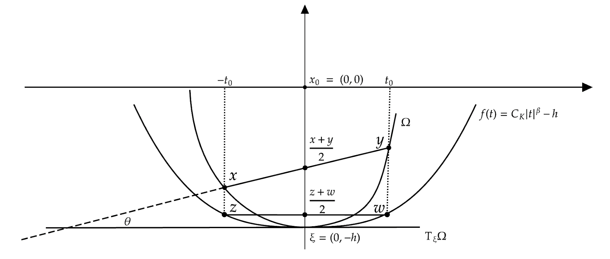
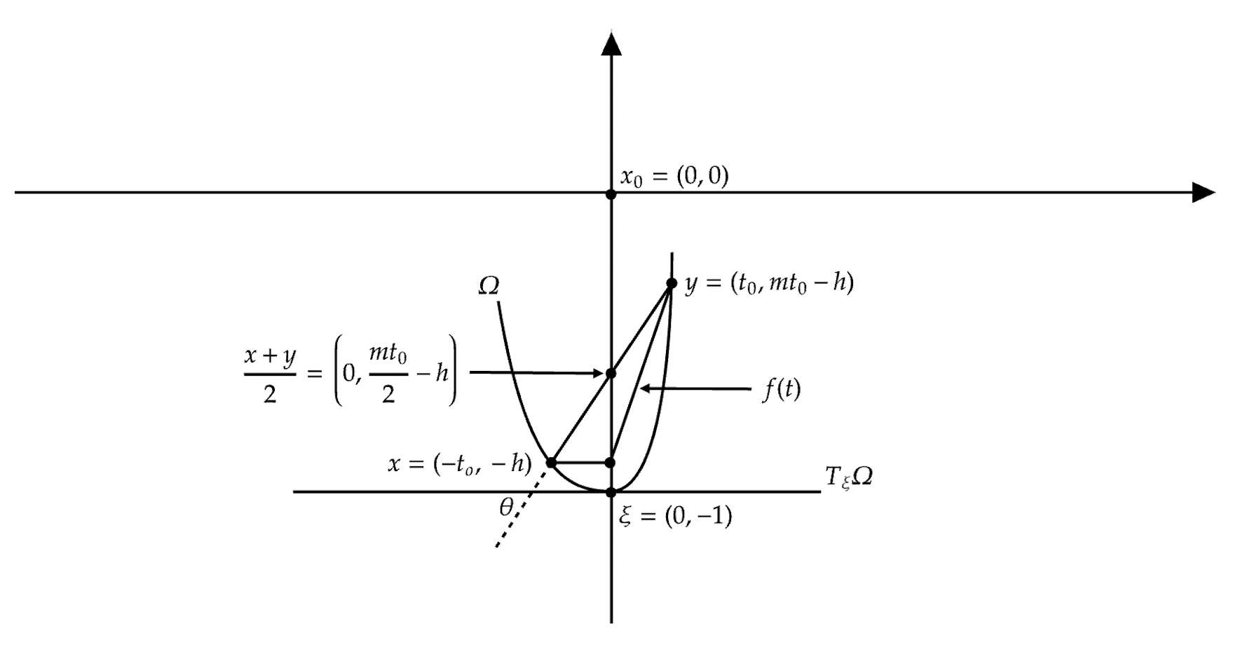
Since is -convex, we have that is bounded below by for some constants and , with both curves meeting at . We denote by the modulus of convexity of , and define and as the vertical projections onto of and , respectively, as shown in Figure 1. Since , we proceed by computing in order to bound from below.
without loss of generality we have , and so . Then by 4.5,
(4.7)
and
(4.8)
Then
(4.9)
∎
5. -Uniform Convexity of the Hilbert metric?
For narrative resolution it would be satisfying to prove that the Hilbert metric on a divisible convex set has -uniformly convex behavior. Toward this end, Ohta’s generalization of 2-uniform convexity for a nonlinear metric space may be useful.
Let be a nonlinear metric space. Then is 2-uniformly convex if for any and any minimal geodesic , we have
(5.1)
Remark 5.2.
When , Equation 5.1 corresponds to the CAT(0) property.
We then have the following question.
Question 5.3.
Let be a strictly convex divisible domain with the Hilbert metric . Is -uniformly convex?
To answer Question 5.3, it would likely be necessary to prove that is uniformly -uniformly convex, i.e. that with independent of the choice of basepoint .
References
[BCL94]
Keith Ball, Eric A. Carlen, and Elliott H. Lieb.
Sharp uniform convexity and smoothness inequalities for trace norms.
Invent. Math., 115(3):463–482, 1994.
[Ben08]
Yves Benoist.
A survey on divisible convex sets.
In Geometry, analysis and topology of discrete groups, volume 6 of Adv. Lect. Math. (ALM), pages 1–18. Int. Press, Somerville, MA, 2008.
[Gui05]
Olivier Guichard.
Sur la régularité Hölder des convexes divisibles.
Ergodic Theory Dynam. Systems, 25(6):1857–1880, 2005.
[KS58]
Paul Kelly and Ernst Straus.
Curvature in hilbert geometries.
Pacific J. Math, 8:119–125, 1958.
[Mar14]
Ludovic Marquis.
Around groups in Hilbert geometry.
In Handbook of Hilbert geometry, volume 22 of IRMA Lect. Math. Theor. Phys., pages 207–261. Eur. Math. Soc., Zürich, 2014.
[Oht09]
Shin-ichi Ohta.
Uniform convexity and smoothness, and their applications in Finsler geometry.
Math. Ann., 343(3):669–699, 2009.
[Suz14]
Tomonari Suzuki.
-uniform convexity and -uniform smoothness of absolute normalized norms on .
Abstr. Appl. Anal., pages Art. ID 746309, 9, 2014.