latex‘!h’ float specifier changed to ‘!ht’
Understanding the Effect of GCN Convolutions
in Regression Tasks
Abstract
Graph Convolutional Networks (GCNs) have become a pivotal method in machine learning for modeling functions over graphs. Despite their widespread success across various applications, their statistical properties (e.g. consistency, convergence rates) remain ill-characterized. To begin addressing this knowledge gap, in this paper, we provide a formal analysis of the impact of convolution operators on regression tasks over homophilic networks. Focusing on estimators based solely on neighborhood aggregation, we examine how two common convolutions—the original GCN and GraphSage convolutions—affect the learning error as a function of the neighborhood topology and the number of convolutional layers. We explicitly characterize the bias-variance trade-off incurred by GCNs as a function of the neighborhood size and identify specific graph topologies where convolution operators are less effective. Our theoretical findings are corroborated by synthetic experiments, and provide a start to a deeper quantitative understanding of convolutional effects in GCNs for offering rigorous guidelines for practitioners.
1 Introduction
Graph Convolutional Networks (GCNs [10, 17]) have become one of the preferred tools for modeling, analyzing, and predicting signals on graphs. Despite their impressive success on academic benchmarks, several fundamental issues limit their broader applicability and reliability in real-world scenarios. In particular, while graphs are highly diverse in their properties (e.g., sparsity, degree distribution, node feature types) and the relationships they encode, GCNs are often suggested as a one-size-fits-all approach. This leaves practitioners with the challenge of selecting an appropriate GCN convolution and architecture for their specific task. Without a clear understanding of the inductive biases these convolutions encode and their expected performance in relation to dataset properties, choosing among the 66 available convolution options in pytorch geometric [25] can become a daunting task. To begin bridging this knowledge gap, this paper investigates the properties of graph convolutions, and relates it to graph or neighborhood properties, focusing specifically on regression tasks over networks.
Statistical Setting.
In this paper, we consider the problem of network regression under fixed design. Let denote a graph with vertex set and edge set . Assume that at each node , we observe a corresponding real-valued response variable , which is generated according to the following mechanism:
| (1) |
where the noise variables are assumed to be uncorrelated, centered, and have variance equal to one. Let denote the vector of responses from all nodes in the graph , the noise vector, and the regression vector. Our goal is to recover from the observations . We also assume that is a homopholic graph, so that neighboring nodes are expected to have similar signal: , if
To reconstruct , a possible solution is to minimize the least squares objective:
with a prespecified function class. To incorporate information about the graph, graph-based regularization methods consider instead a penalized objective of the form:
where Pen denotes a function penalizing differences along edges of the graph.
When the graph is endowed with node features , and the estimator is chosen to be a function of these features (e.g. ), the task is usually known as node regression. When the estimator is constructed using information solely from the observed values of , the problem boils down to a denoising task usually known as graph-trend filtering [15, 35], an extension of the classical Gaussian Sequence model [26, 36] to accommodate graph structure. In this paper, we aim to study the performance of graph convolutionals to provide reliable estimates for in the denoising setting.
Notations.
Let represent the cardinality of a set . We denote a graph with vertex set and edge set by . Without loss of generality, we assume that the vertices are indexed from 1 to , so and . Let denote the binary adjacency matrix, which encodes the edge structure of the graph as follows:
For any , we further denote by all nodes that are at most hops away from node . We denote the neighborhood of node by . Note that . For any , let denote the edge degree of node , specifically . The degree matrix is the diagonal matrix with diagonal entries
The graph Laplacian is denoted by
and is a positive semi-definite and symmetric matrix [4]. For a vector , denotes the squared Euclidean norm and the notation represents the -th component of the vector. For a square matrix , let denote the Frobenius norm and denote the trace.
Related literature.
The theory for node regression has been derived from different viewpoints. Asymptotic viewpoint assumes that the number of vertices tends to infinity, so that the Laplacian matrix is used to approximate the Laplace-Beltrami operator on an underlying manifold [1, 19, 29] on which the function is assumed to be smooth [11, 34]. Instead of assuming a growing graph, one can alternatively work with a fixed graph where, for a randomly selected subset of nodes, the response vectors are masked/unobserved [17, 6]. A typical assumption consists in assuming that neighboring nodes will have the same response – in other words, assuming that the graph is homophilic. In this setting, several strategies leveraging the graph structure to guide the inference can be deployed: (a) Laplacian regularization, (b) regularization and (c) graph convolutions.
Laplacian regularization (also known as Laplacian smoothing [30], a special instance of Tikhonov regularisation) is perhaps one of the better studied version of the problem. As described in a previous paragraph, these methods usually consider a smooth function (where the smoothness of the function is consequently defined via the eigenvalue decay of the graph Laplacian), and use the convergence of the graph Laplacian to the Laplace-Beltrami operator to establish the consistency and convergence rates of the proposed estimator [11, 34]. Several research groups have explored similar concepts. [2] provides bounds on the generalization error for Tikhonov regularization and interpolated regularization. Work by [18] derives posterior contraction rates for using a Bayesian formalism. The rates depend on the eigenvalue decay of the graph Laplacian and a smoothness index that is defined via a Sobolev-type space based on the graph Laplacian. More recently, work by Green and coauthors [8, 9] derives optimal convergence rates for Laplacian-based regularization in the fixed design setting.
Graph-trend filtering (also known as “graph total-variation” or “fused lasso”) estimators use an penalty to guide the inference, so that estimators are derived as the solution of the following optimisation problem:
Recent work, see [15, 24] has characterized the convergence rate of these estimators as a function of the underlying graph smoothness, defined this time in the amount of variation registered along the graph edges: While this approach is attractive for approximative near piece-wise constant functions over graphs, estimators are often more computational intensive than Laplacian based estimators.
Finally, Graph Convolution Neural Networks [17] are a more recent addition to the set of methods. While typically used for classification, this method is increasingly used for node regression tasks. The theoretical understanding of GCNs models remains quite limited. For example, [32] analyses the stability of single-layer GCNs models and derives their generalization guarantees, showing that, in regression problems, the generalization gap between training error and testing error decreases at a sub-linear rate as the number of training samples increases. The work in [12, 5] demonstrates that GCNs can be interpreted as a simplification of spectral-type GNNs that utilize the graph Laplacian. In [20], it is shown that graph convolution is essentially a form of Laplacian smoothing. [33] investigates the classification performance of graph neural networks with graph-polynomial features under a general contextual stochastic block model.
Contrary to earlier work, in this paper we aim to provide statistical insight into the regression setting. We analyze a widely used class of GNNs, Graph Convolutional Networks (GCNs), which we introduce in depth in the next section.
2 Graph convolutional networks (GCNs)
While graph neural networks (GNNs) is a broad term encompassing various network structures for graph learning, graph convolutional networks (GCNs) [17] form a specific class of GNNs. GCNs take the response vector and the adjacency matrix as the input. Let be the number of GCN layers. For each , the output of the layers can be defined recursively via
where is a non-linear function and . In layer , the network has performed a -fold composition of the map and we will set A GCN with layers is then a function
Specific GCN models differ in the choice and parametrization of the function . An important case is the layer-wise propagation rule with of the form
| (2) |
Here, denotes componentwise application of the ReLU activation function, is a weight parameter, and
| (3) |
for the adjacency/degree matrix with added self-loops and that is, and is the diagonal matrix with diagonal entries
The definition can be extended to the case where at each node we do not only observe one number but a feature vector of length . In this case, becomes a matrix and can be chosen as matrix.
The formulation of (2) originates from [17]. Its motivation is to provide a first-order approximation for the localized spectral filters introduced in [5] for signal processing, suggesting that GCNs should be applied in the fixed design framework.
In addition to the widely used propagation operator , this paper also discusses the original normalization approach, that replaces by
| (4) |
If the activation function in (2) is set to the identity function, then the GCN of depth takes on a specific form
| (5) |
with , or , and are the weight parameters in each layer. Empirical studies demonstrate that, compared to nonlinear activation functions (2), linear GCNs as defined in (5) do not have a detrimental effect on accuracy in many downstream applications [37]. In [23], the authors provide theoretical evidence that non-linearity does not enhance the expressive power of GCNs. The linear setting has also been considered in [33] and referred to as poly-GNN. Further discussion comparing linear GCNs to the original GCNs can be found in [21, 22].
Rewriting (5) yields
| (6) |
with some . We denote the class of functions described in (6) as and base our analysis on this class.
The theory of GCNs.
Several studies have begun investigating the capabilities and limitations of Graph Neural Networks (GNNs). Most analyses focus on comparing different classes of GNN architectures using the Weisfeiler-Lemann test to distinguish graph structures [38] or on performance in classification tasks [7]. While issues such as oversmoothing in deeper GNNs have been explored [20, 23], there is a noticeable gap in evaluating the consistency of GNN-based estimators. In particular, little has been done to analyze the bias-variance trade-off concerning neighborhood size and topology. This gap highlights the need for a deeper understanding of how graph convolution operations affect the statistical properties of GNNs, motivating our investigation.
3 Theoretical results for deep linear GCNs
GCNs incorporate the graph information in the layers and do not require any penalization. Instead, it is sufficient to minimize the least-squares objective over the class of GCNs,
with
where the equality follows by minimizing over the GCN parameter in (6). This estimator denoises by regressing it on itself and neighboring nodes. The size of the neighborhood is controlled by the depth
To understand the role of the parameter in the GCN, we disregard its randomness and focus on a fixed parameter For any matrix using that the measurement noise in Model (1) is centered and the triangle inequality, we then obtain the bias-variance type decomposition
| (7) |
Optimizing over the parameter balances squared bias and variance. In case of a small signal the optimal will be in and induces thus shrinkage. An extreme case is Choosing will then lead to vanishing mean squared error.
In nonparametric statistics, the convergence rates of an estimator depends on the smoothness of the regression function. In the context of graphs, this smoothness is naturally expressed in terms of the neighborhood structure. As mentioned in the statistical setting, we consider a homophilic graph meaning that neighboring nodes are expected to have similar signals . However, the specific similarity assumption concerning neighboring nodes depends on the graph aggregation operator , which incorporates various normalization approaches. We present these formally as follows.
Assumption 1.
There exists a such that for any and any
| (8) |
and
| (9) |
Recall that denotes the Frobenius norm of a matrix, while represents the number of edges in the graph The subsequent result bounds the mean squared error by a squared bias and a variance term.
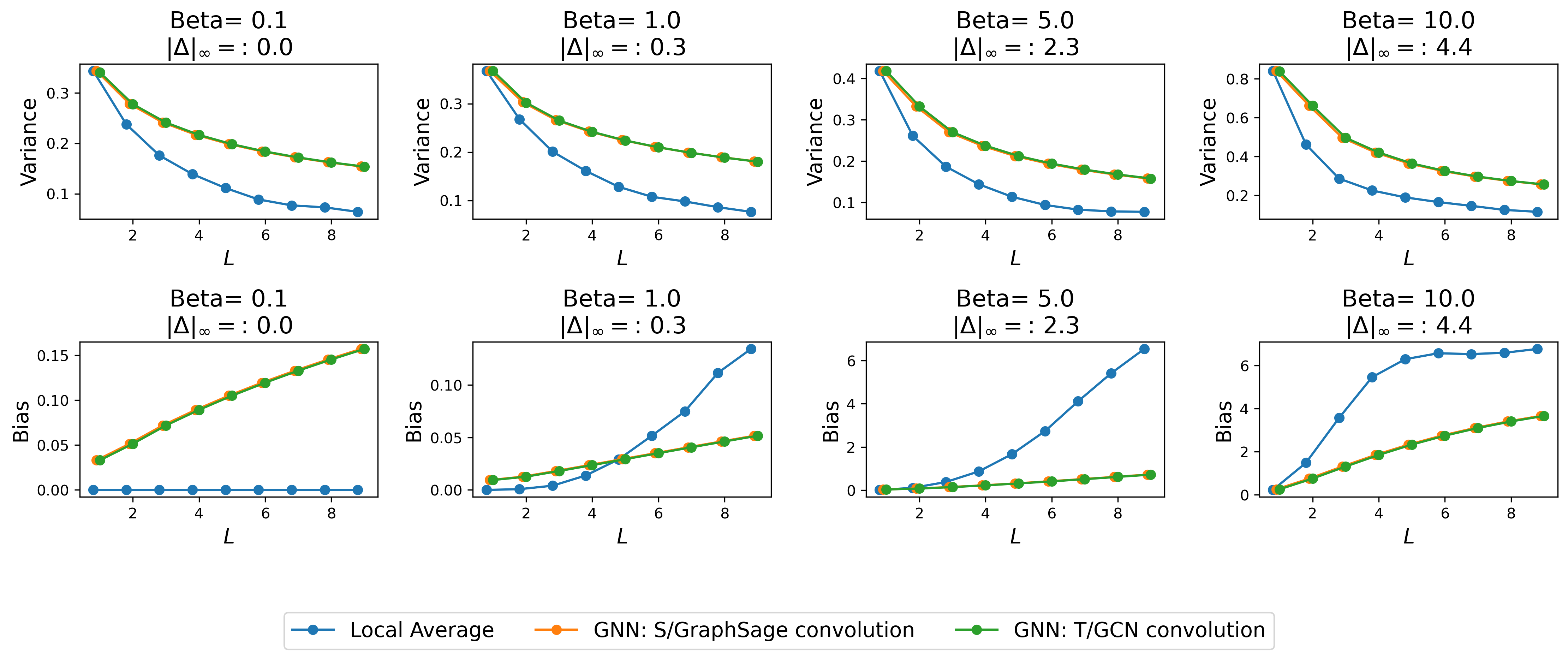
While the bias term will increase in the depth we will show that the variance term can quickly decrease in This elucidates why, in practical applications, there is an optimal layer for implementing linear GCNs. This finding will also be further validated and demonstrated in the experimental study section (see Figure 1 in Section 4).
Besides this bias-variance trade-off phenomenon involving , the variance decay can exhibit significantly different behaviors depending on the specific structure of the graph . Even within a single fixed graph, nodes with distinct local features may exhibit varying patterns of variance decay, which we will discuss in more detail shortly.
GCNs with linear layers denoise the response variables by averaging over neighboring nodes. A natural competitor is the estimator that estimates the -th signal by uniformly averaging over the set denoting the neighboring nodes within a distance of at most from node . Writing for its cardinality, the local average estimator is
| (12) |
with
| (13) |
Theorem 2.
For the variance of each is given by . If (8) holds, then
| (14) |
If we compare the upper bounds given by Theorems 1 and 2, we see that the bias term in (10) can be smaller depending on . We analyse the variance term in details in the next session.
3.1 Bounds for the variance via weighted local walks on the graph
We now examine the dependence of the network depth on the variance decay for different local graph topologies and the graph aggregation operators and .
The definition of in (3) and in (4) are based on the adjacency matrix with added self-loops While the original graph is denoted by , we write for the graph augmented with self-loops. Recall that the edge degrees of the graph are denoted by A path from node to node via nodes is denoted by
The length of the path is We associate to this path the weights
and
| (15) |
Let denote all paths from node to node of length in the self-loop augmented graph There is a one-to-one correspondence with the paths from to of length in the original graph The key observation is that for any vector
and
see also the supplement for a derivation.
Since the noise vector consists of centered and uncorrelated random variables with variance one, we find
and
The edge degrees and the length of the paths decrease the weights but increase the number of paths. Interestingly, the variance can exhibit significantly different behaviors depending on the local graph structure around node . In the following, we primarily focus on the analysis for the case . The results for are similar to those for due to the connection in (15); therefore, we have included the corresponding results and proofs in the Appendix.
Since the row sums of the matrix are all one, is a transition matrix of a Markov chain. Thus, is a transition matrix with row sums equal to one and for any node
Recall that and denote the set of neighboring nodes within a distance of at most from node and its cardinality. In the previous display, can be replaced by Applying the Cauchy-Schwarz inequality (AM-QM) and Theorem 2, we deduce
| (16) |
For equality holds in (16). The inequality shows that, in general, the local averaging estimator has smaller variance if we take the same in the GCN estimator and the local averaging estimator. On the contrary, the GCN estimator is expected to have a smaller bias, as it computes a weighted sum over the local neighborhood assigning more mass to nodes that are closer to in path distance. Although the gain in the bias is hard to quantify theoretically, we see that it outweighs the loss in the variance in our empirical studies. For instance, in all the scenarios in Figure 4 the GCN estimator has smaller test error.
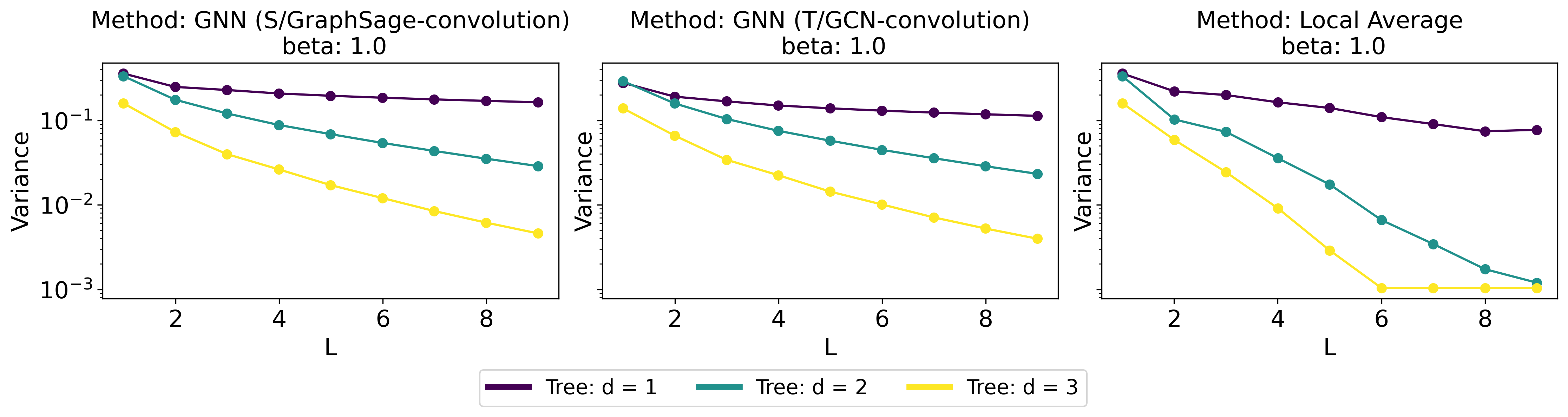
We now provide an upper bound assuming that node is the root of a locally-rooted tree. In this scenario, the variance term decays exponentially in the number of layers (see Figure 2).
Proposition 1.
Assume the local graph around node is a rooted tree, in the sense that the subgraph induced by the vertices forms a rooted tree with root and all nodes having edge degree . Then, we have
In this case, the variance decay in is This is the sharp rate, since the lower bound in (16) gives the same rate, namely
A slow rate of the variance term occurs if node has edge degree say but is connected to nodes with small edge degree.
Proposition 2.
If there exists a path from node to node via nodes such that then
This indicates that under this scenario, the decay of the variance term in is significantly slower than
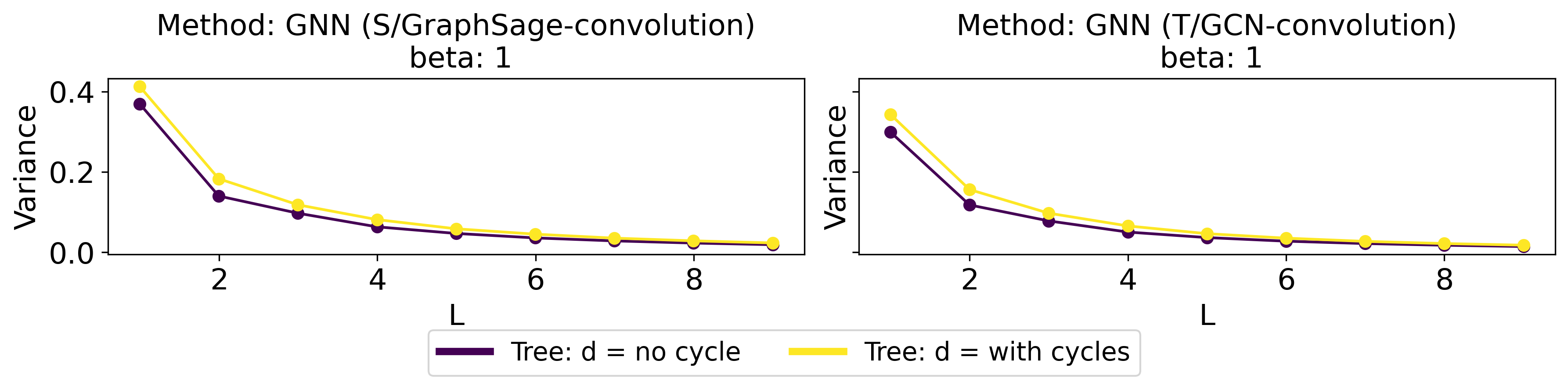
Aside from the tree structure, the decay of the variance term can suddenly exhibit slow decay once an additional cycle is attached to some node in the graph .
Proposition 3.
Assume that the graph decomposes into a cycle of length and a graph in the sense that and share exactly one node and there are no edges connecting and Then, for any ,
| (17) |
The variance term in GCNs is sensitive to small perturbations in the graph. To see this, suppose node admits a local tree structure as described in Proposition 1. Attaching an additional cycle to node , (17) demonstrates that regardless of the edge degree of node , the variance decay rate in will immediately drop from to . On the contrary, the local average estimator (12) will hardly be affected by an additional cycle.
In practical applications, such as social network analysis, it is common to observe nodes exhibiting an additional cycle, or even multiple ones. Once a cycle is attached to some nodes, the variance decay slows down. However, increasing the number of convolutional layers may also increase the bias, as indicated by a combination of Theorem 1 and Proposition 3. Our example serves as a prototype to demonstrate why, in practice, simply stacking the layers of a GCN leads to poor performance for the resulting estimator. This phenomenon, known as over-smoothing in GCN literature [23, 3, 27, 20], contrasts with Fully Connected Neural Networks (FNNs), where theory and evidence suggest that greater depth improves representation power [31, 28]. In [23, 3], the over-smoothing phenomenon is studied asymptotically, assuming the number of layers tends to infinity. Some results in [23] also rely on large graphs with being large. Our result, established in a non-asymptotic regression setting, differs from most existing work focused on node classification. By starting with a bias-variance decomposition and analyzing weighted local walks on the graph, we quantitatively uncover the underlying reasons for this phenomenon, offering insights for improving GCNs in practice.
4 Numerical simulations
We validate our results through a set of numerical experiments. Specifically, to evaluate the link between neighborhood topology — particularly degree distribution and degree skewness — and optimal neighborhood size, we generate graphs with nodes using the following topologies:
-
•
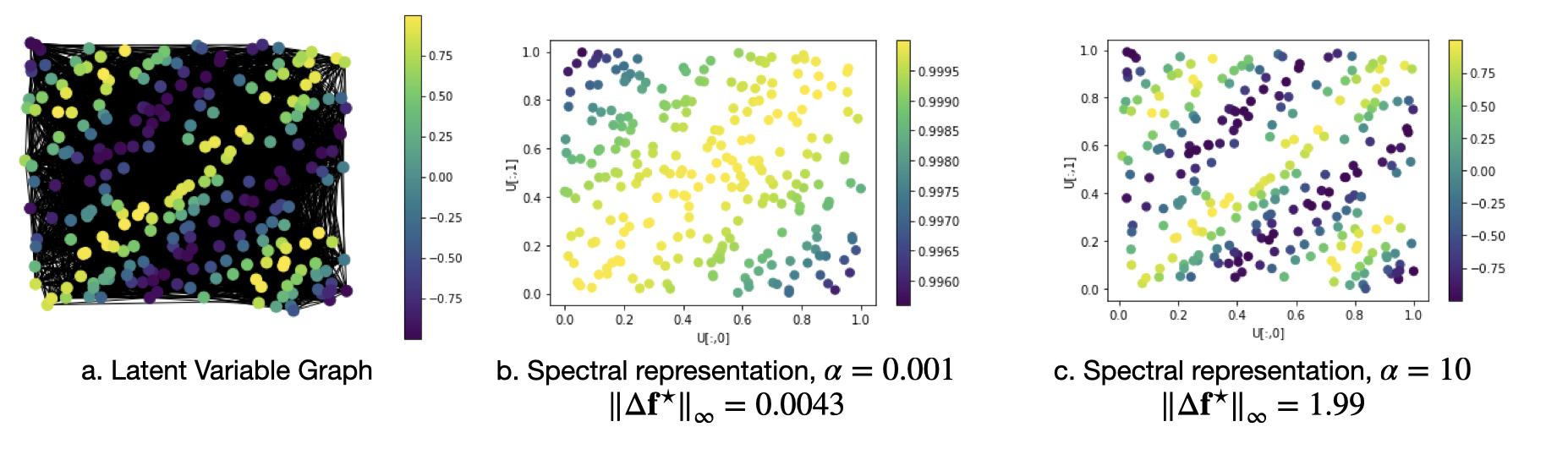
Latent variable graphs: we generate latent variables for nodes by drawing dimensional latent variables from a uniform distribution. The edges of the network are then sampled from a Bernoulli distribution with , where the scaling factor is chosen empirically to control the edge density. To further measure the effect of the density of the network on the optimal neighborhood size, we sparsify the induced network as follows. To ensure the connectedness of the graph, we first sample a minimum spanning tree. We then delete edges that are not in the MST with probability , so that a higher results in a sparser graph. The resulting sparsity of the graph is highlighted in Table 1 in the Appendix.
-
•
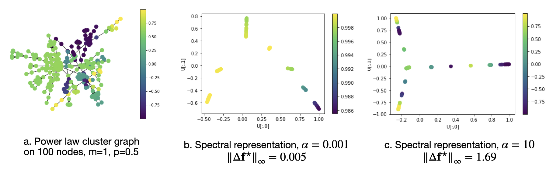
Preferential attachment graphs using the Holme and Kim algorithm [13], varying their local clustering probability . In this case, higher values of yield graphs with higher clustering coefficients.
-
•
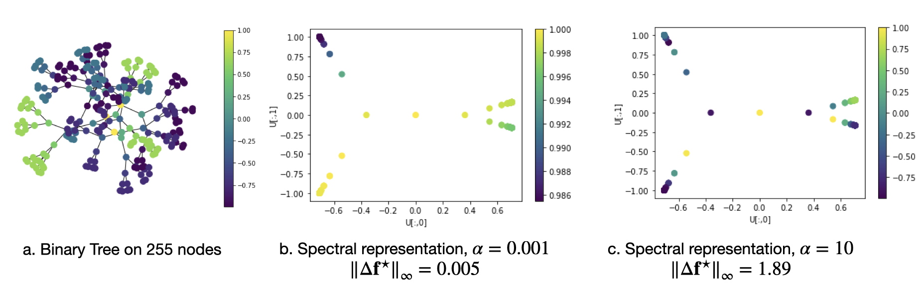
k-regular trees, where denotes the degree of each node in the tree.
-
•
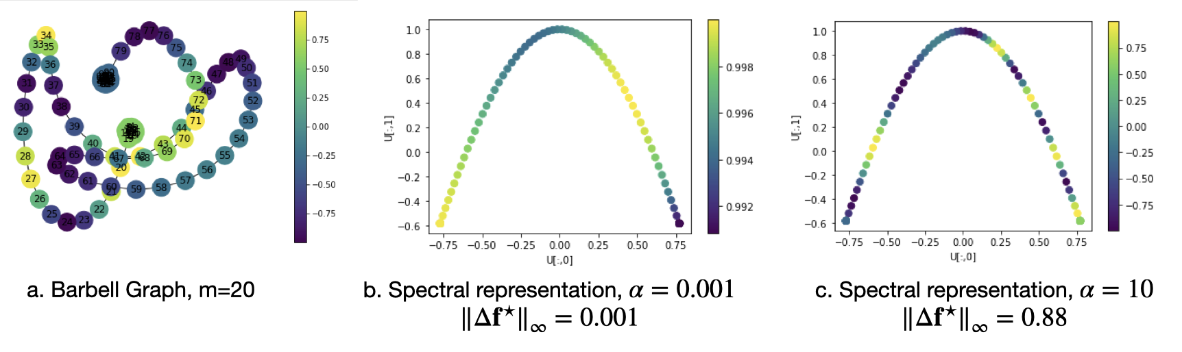
Barbell graphs, consisting of two cliques of fully connected nodes, joined by a chain on nodes.
In the first case, the signal is created as a smooth function of the latent variable : , with a coefficient of the form , where is adjusted to control different levels of smoothness across the graph: as highlighted in Figure 1 in the Appendix, lower values of tend to create smooth functions, while higher values of induce faster varying signals. In the three other cases, the signal is created in a similar fashion, replacing the latent variables with the first two eigenvectors of the graph Laplacian. An example of our generation setup is provided in the Appendix.
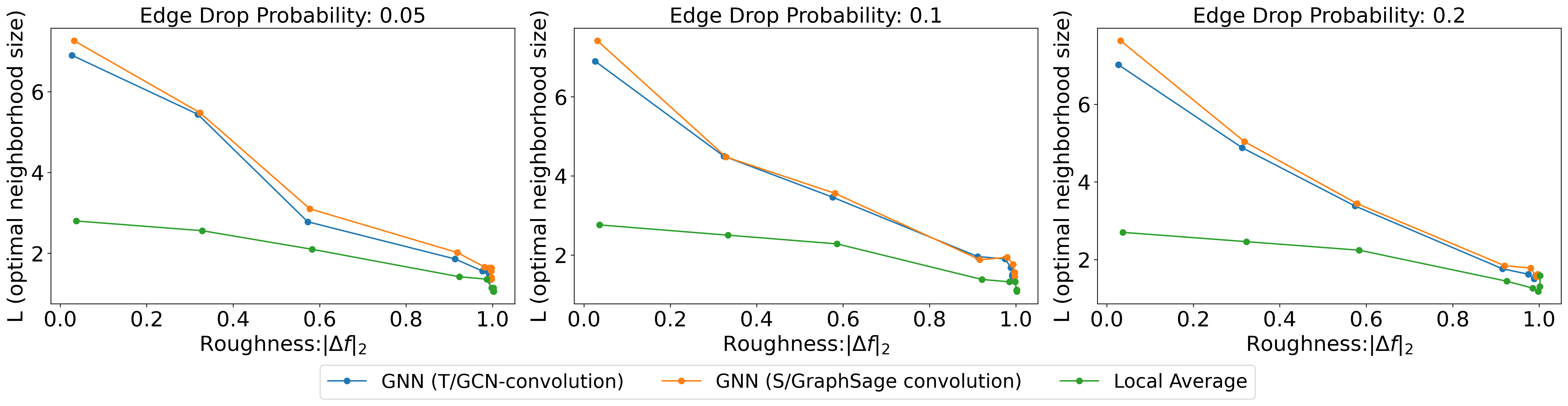
Results
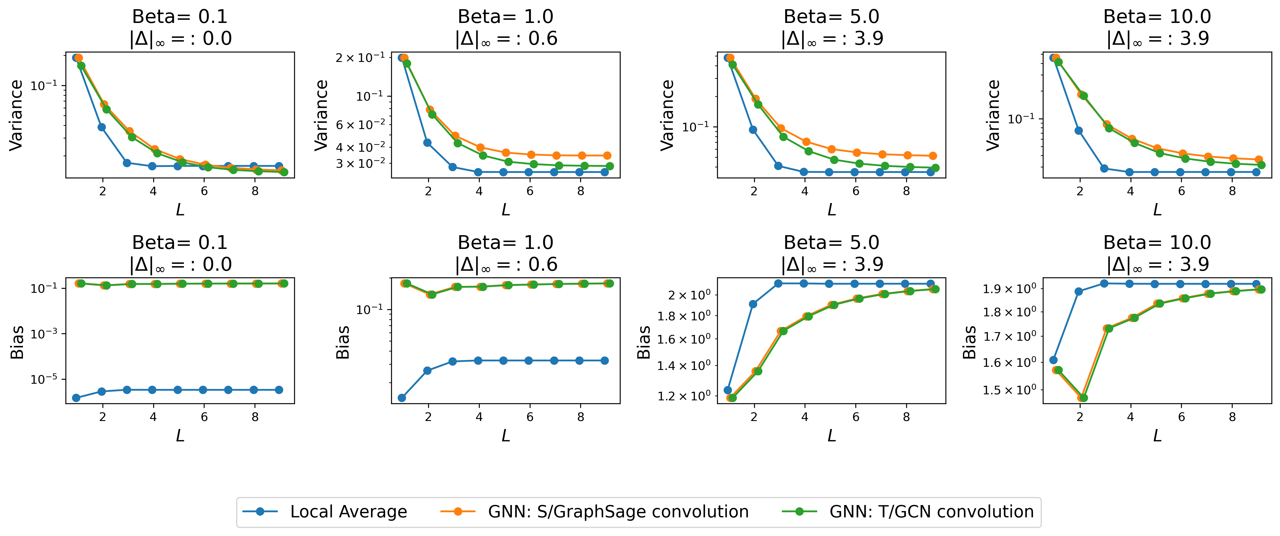
The results for the various topologies are provided in the Appendix. Overall, the optimal number of convolutions seems to be dependent on the local topology of the node’s neighborhood. We also assess the decay rate of the variance in rooted trees as a function of the degree. As detailed in Proposition 1, we expect the variance decay to be larger as increases. Figure 2 shows the decay of the squared bias and variance as a function of (the neighborhood depth, here logged on the x-axis) for where controls the smoothness of the function . As expected, we note that the log of the variance decays as a linear function of the number of convolutions , with higher degrees yielding higher decay slopes.
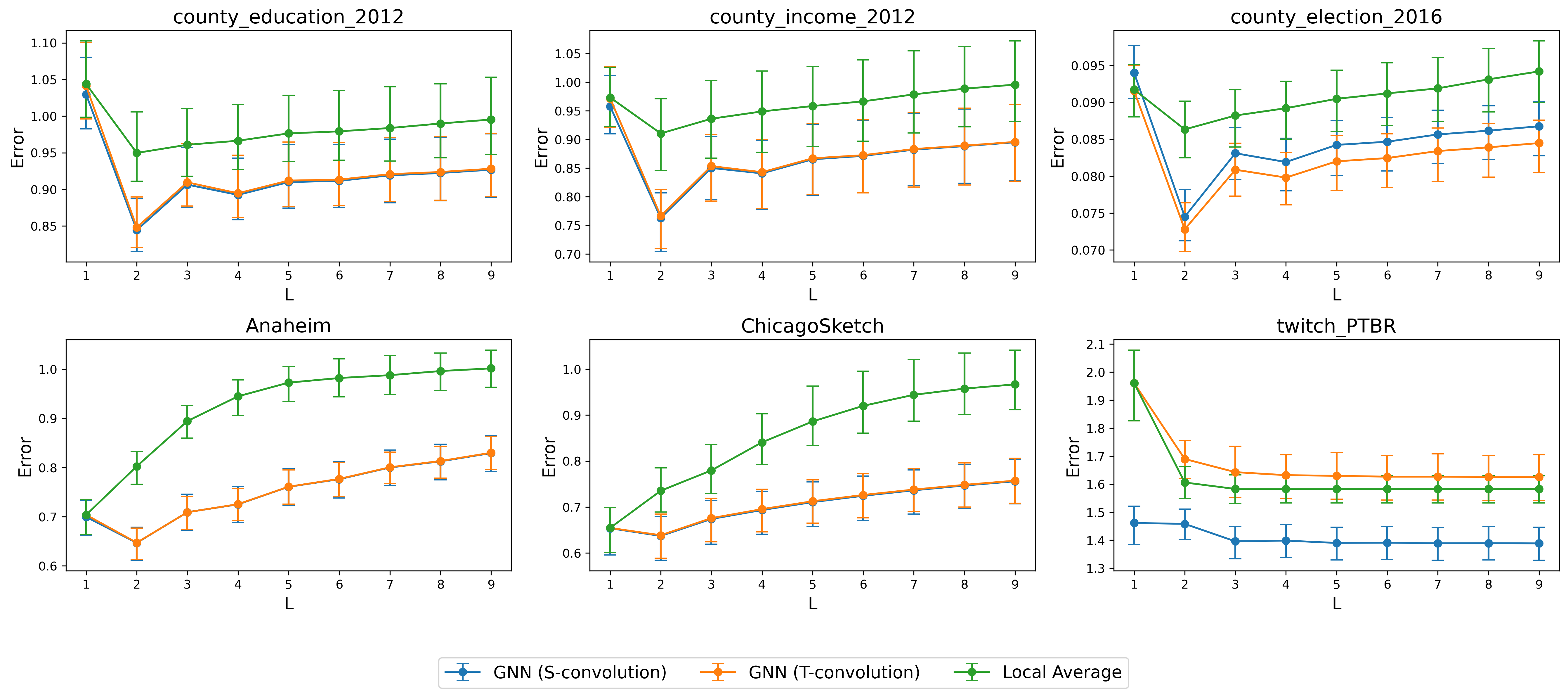
5 Real-data analysis
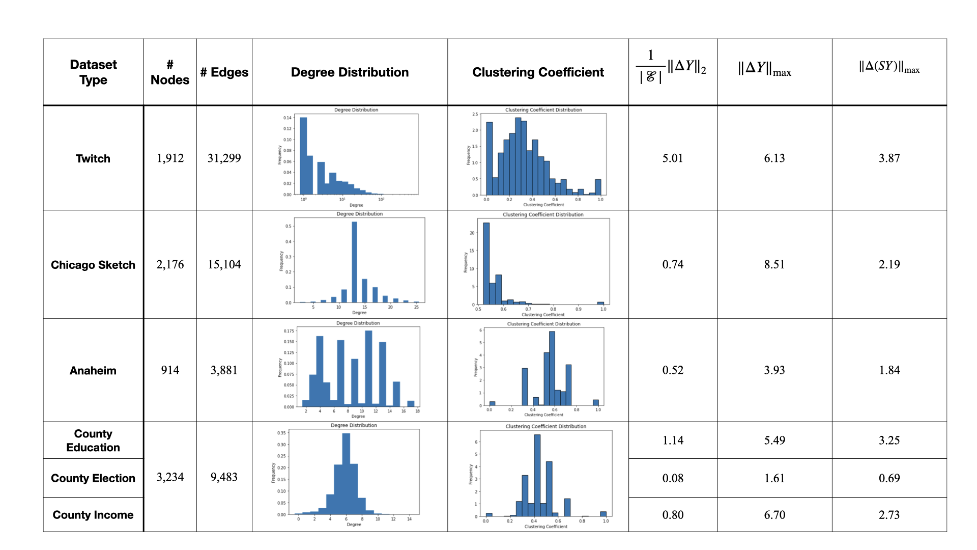
We validate our framework on 6 real-world examples. More specifically, we used the publicly available regression datasets used as validation by [16] and [14]. These datasets include 4 spatial datasets on election results, income, unemployment as well as education levels across the counties in the US. These datasets also include 2 transportation networks, based on traffic data in the cities of Anaheim and Chicago. Each vertex represents a directed lane, and two lanes that meet at the same intersection are connected. In these datasets, the signal represents the traffic flow in the lane. Finally, the Twitch dataset captures friendships amongst Twitch streamers in Portugal, while the node signal corresponds to the logarithm of the number of viewers for each streamer. A table listing the datasets and their properties can be found in the Appendix, highlighting the different topological characteristics of these datasets. In particular, spatial datasets tend to have a regular degree, while the degree distribution is highly skewed in the twitch datasets.
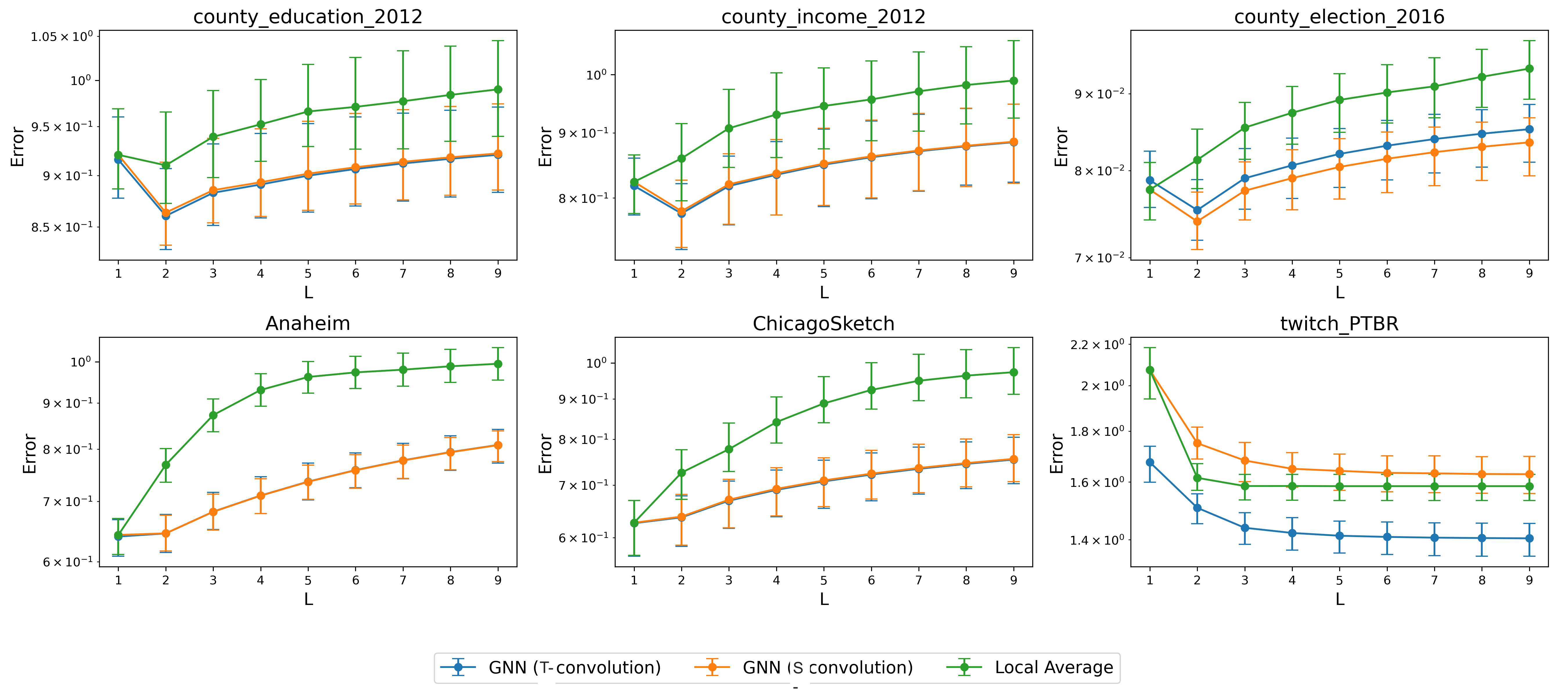
We use our estimator in the prediction setting, where the value at the node of interest is unobserved. To this end, we select at random a set of 500 nodes for training (i.e. selection of the most appropriate value of neighborhood size ) and 500 for validation. Figure 4 shows the MSE error as a function of the neighborhood size. Interestingly, we note that the optimal neighborhood size is reached at for all spatial graphs. In these settings, the degree distribution is relatively homogeneous across the nodes (see statistics in the Appendix), and the convolutions and give reasonably similar results. Interestingly, however, in the social network example, the convolution yields drastically different effects.
We also test our estimator in the denoising setting. To avoid data snooping, we replace the value at the selected nodes with one of their direct neighbours. In the homophilic graph setting, this is indeed akin to assuming that direct neighbours have roughly the same distribution of the node of interest. Therefore, replacing the node by one of its neighbors ensures that we are generating an independent copy of the graph with the same distribution. The results are presented in the Appendix.
6 Discussion
In this work we pave the way towards a statistical foundation of graph convolutional networks (GCNs). Graph convolutional networks perform weighted local averaging over neighboring nodes where the neighborhood size is controlled by the depth of the GCN. Studying node regression, we showed that the variance of the GCN is a weighted sum over paths. This link allows to derive lower and upper bounds of the variance based on local graph properties. Our analysis reveals some non-robustness of GCNs in the sense that small perturbations of these graph properties can lead to huge changes in the variance.
Acknowledgements
The research of J. S.-H. and J. C. was supported by the NWO Vidi grant VI.Vidi.192.021. The research of C. D. was funded by the National Science Foundation (Award Number 2238616), as well as the resources provided by the University of Chicago’s Research Computing Center. The work of O. K. was funded by CY Initiative (grant “Investissements d’Avenir” ANR-16-IDEX0008) and Labex MME-DII(ANR11-LBX-0023-01).
References
- Belkin and Niyogi [2003] Mikhail Belkin and Partha Niyogi. Laplacian eigenmaps for dimensionality reduction and data representation. Neural computation, 15(6):1373–1396, 2003.
- Belkin et al. [2004] Mikhail Belkin, Irina Matveeva, and Partha Niyogi. Regularization and semi-supervised learning on large graphs. In Conference on Learning Theory (COLT), pages 624–638, 2004.
- Cai and Wang [2020] Chen Cai and Yusu Wang. A note on over-smoothing for graph neural networks. arXiv preprint arXiv:2006.13318, 2020.
- Chung [1996] Fan R. K. Chung. Lectures on spectral graph theory. CBMS Lectures, Fresno, 6(92):17–21, 1996.
- Defferrard et al. [2016] Michaël Defferrard, Xavier Bresson, and Pierre Vandergheynst. Convolutional neural networks on graphs with fast localized spectral filtering. In Neural Information Processing Systems (NeurIPS), pages 3844–3852, 2016.
- Donnat et al. [2024] Claire Donnat, Olga Klopp, and Nicolas Verzelen. One-bit total variation denoising over networks with applications to partially observed epidemics. arXiv preprint arXiv:2405.00619, 2024.
- Garg et al. [2020] Vikas Garg, Stefanie Jegelka, and Tommi Jaakkola. Generalization and representational limits of graph neural networks. In International Conference on Machine Learning (ICML), pages 3419–3430, 2020.
- Green et al. [2021] Alden Green, Sivaraman Balakrishnan, and Ryan Tibshirani. Minimax optimal regression over Sobolev spaces via Laplacian regularization on neighborhood graphs. In International Conference on Artificial Intelligence and Statistics (AIStats), pages 2602–2610, 2021.
- Green et al. [2023] Alden Green, Sivaraman Balakrishnan, and Ryan J Tibshirani. Minimax optimal regression over Sobolev spaces via Laplacian Eigenmaps on neighbourhood graphs. Information and Inference: A Journal of the IMA, 12(3):2423–2502, 2023.
- Hamilton et al. [2017] William L Hamilton, Rex Ying, and Jure Leskovec. Inductive representation learning on large graphs. arXiv preprint arXiv:1706.02216, 2017.
- Hein [2006] Matthias Hein. Uniform convergence of adaptive graph-based regularization. In Conference on Learning Theory (COLT), pages 50–64, 2006.
- Henaff et al. [2015] Mikael Henaff, Joan Bruna, and Yann LeCun. Deep convolutional networks on graph-structured data. arXiv preprint arXiv:1506.05163, 2015.
- Holme and Kim [2002] Petter Holme and Beom Jun Kim. Growing scale-free networks with tunable clustering. Physical review E, 65(2):026107, 2002.
- Huang et al. [2024] Kexin Huang, Ying Jin, Emmanuel Candes, and Jure Leskovec. Uncertainty quantification over graph with conformalized graph neural networks. In Neural Information Processing Systems (NeurIPS), volume 36, 2024.
- Hütter and Rigollet [2016] Jan-Christian Hütter and Philippe Rigollet. Optimal rates for total variation denoising. In Conference on Learning Theory (COLT), pages 1115–1146, 2016.
- Jia and Benson [2020] Junteng Jia and Austion R Benson. Residual correlation in graph neural network regression. In Proceedings of the 26th ACM SIGKDD International Conference on Knowledge Discovery & Data Mining, pages 588–598, 2020.
- Kipf and Welling [2017] Thomas N. Kipf and Max Welling. Semi-supervised classification with graph convolutional networks. In International Conference on Learning Representations (ICLR), 2017.
- Kirichenko and van Zanten [2017] Alisa Kirichenko and Harry van Zanten. Estimating a smooth function on a large graph by Bayesian Laplacian regularisation. Electronic Journal of Statistics, 11(1):891–915, 2017.
- Lafon [2004] Stéphane S Lafon. Diffusion maps and geometric harmonics. Yale University, 2004.
- Li et al. [2018] Qimai Li, Zhichao Han, and Xiao-Ming Wu. Deeper insights into graph convolutional networks for semi-supervised learning. In AAAI Conference on Artificial Intelligence, 2018.
- NT and Maehara [2019] Hoang NT and Takanori Maehara. Revisiting graph neural networks: All we have is low-pass filters. arXiv preprint arXiv:1905.09550, 2019.
- NT et al. [2021] Hoang NT, Takanori Maehara, and Tsuyoshi Murata. Revisiting graph neural networks: Graph filtering perspective. In International Conference on Pattern Recognition (ICPR), pages 8376–8383, 2021.
- Oono and Suzuki [2020] Kenta Oono and Taiji Suzuki. Graph neural networks exponentially lose expressive power for node classification. In International Conference on Learning Representations (ICLR), 2020. URL https://openreview.net/forum?id=S1ldO2EFPr.
- Padilla et al. [2018] Oscar Hernan Madrid Padilla, James Sharpnack, James G. Scott, and Ryan J. Tibshirani. The DFS Fused Lasso: Linear-time denoising over general graphs. Journal of Machine Learning Research, 18(176):1–36, 2018. ISSN 1533-7928. URL http://jmlr.org/papers/v18/16-532.html.
- Paszke et al. [2019] Adam Paszke, Sam Gross, Francisco Massa, Adam Lerer, James Bradbury, Gregory Chanan, Trevor Killeen, Zeming Lin, Natalia Gimelshein, Luca Antiga, Alban Desmaison, Andreas Kopf, Edward Yang, Zachary DeVito, Martin Raison, Alykhan Tejani, Sasank Chilamkurthy, Benoit Steiner, Lu Fang, Junjie Bai, and Soumith Chintala. Pytorch: An imperative style, high-performance deep learning library. In Neural Information Processing Systems (NeurIPS), 2019.
- Rigollet [2015] Philippe Rigollet. High-dimensional statistics. Lecture Notes, Cambridge, MA, USA: MIT Open-CourseWare, 2015.
- Rusch et al. [2023] T. Konstantin Rusch, Michael M. Bronstein, and Siddhartha Mishra. A survey on oversmoothing in graph neural networks. arXiv preprint arXiv:2303.10993, 2023.
- Schmidt-Hieber [2020] Johannes Schmidt-Hieber. Nonparametric regression using deep neural networks with ReLU activation function. The Annals of Statistics, 48(4):1875 – 1897, 2020. doi: 10.1214/19-AOS1875. URL https://doi.org/10.1214/19-AOS1875.
- Singer [2006] Amit Singer. From graph to manifold Laplacian: The convergence rate. Applied and Computational Harmonic Analysis, 21(1):128–134, 2006.
- Smola and Kondor [2003] Alexander J. Smola and Risi Kondor. Kernels and regularization on graphs. In Conference on Learning Theory (COLT), pages 144–158, 2003.
- Telgarsky [2016] Matus Telgarsky. Benefits of depth in neural networks. In Conference on Learning Theory (COLT), pages 1517–1539, 2016.
- Verma and Zhang [2019] Saurabh Verma and Zhi-Li Zhang. Stability and generalization of graph convolutional neural networks. In ACM SIGKDD International Conference on Knowledge Discovery & Data Mining, pages 1539–1548, 2019.
- Vinas and Amini [2024] Lucian Vinas and Arash A. Amini. Sharp bounds for Poly-GNNs and the effect of graph noise. arXiv preprint arXiv:2407.19567, 2024.
- Von Luxburg et al. [2008] Ulrike Von Luxburg, Mikhail Belkin, and Olivier Bousquet. Consistency of spectral clustering. The Annals of Statistics, pages 555–586, 2008.
- Wang et al. [2016] Yu-Xiang Wang, James Sharpnack, Alexander J Smola, and Ryan J Tibshirani. Trend filtering on graphs. Journal of Machine Learning Research, 17(105):1–41, 2016.
- Wasserman [2006] Larry Wasserman. All of nonparametric statistics. Springer Science & Business Media, 2006.
- Wu et al. [2019] Felix Wu, Amauri Souza, Tianyi Zhang, Christopher Fifty, Tao Yu, and Kilian Weinberger. Simplifying graph convolutional networks. In International Conference on Machine Learning (ICML), pages 6861–6871, 2019.
- Xu et al. [2018] Keyulu Xu, Weihua Hu, Jure Leskovec, and Stefanie Jegelka. How powerful are graph neural networks? arXiv preprint arXiv:1810.00826, 2018.
Appendix A PROOFS OF MAIN THEOREMS
A.1 Proof of Theorem 1
Recall that as the noise is centered, with inequality (7), we have for any fixed parameter and matrix ,
| (1∗) |
We first consider the case for . To further bound (1∗) for , we now prove by induction on that
| (2∗) |
where for any vector .
Write
| (3∗) |
where , for all and , for indicating whether nodes and are connected by an edge belonging to . The matrix represents the connection structure of the augmented graph , where self-loops are included by setting , for . Thus,
| (4∗) |
where is the edge degree of node .
For , we can employ the smoothness condition (8) in Assumption 1 and the fact that the edge degree is the same as the number of neighbors of to show
For the induction step, assume the claim holds until , in the sense that, for any , Then,
completing the induction step. Thus, we conclude that for all . This implies that
| (5∗) |
Moreover, for the variance part, we use the fact that the components of are uncorrelated and have a variance of one to obtain
| (6∗) |
Plugging (5∗) and (6∗) into (1∗) with , we deduce that
which completes the proof of (10).
A.2 Proof of Theorem 2
By definition (13),
Since the components of are uncorrelated and have a variance of one, we obtain
For any , there exists a path in the augmented graph , where self-loops are allowed, given by
| (10∗) |
which connects node to node through nodes and has a length of . The path in (10∗) also implies that . Therefore, if condition (8) in Assumption 1 holds, we have, for any ,
| (11∗) |
Since the noise variables are assumed to be uncorrelated, centered, and have a variance of one, we can derive using (11∗) that for any ,
| (12∗) |
Summing (12∗) for all finally yields
Appendix B DERIVATION OF ASSOCIATED WEIGHTS
B.1 Associated weights for
Recall that we can represent as shown in (4∗), where for indicates whether node is connected to node by an edge in , and since self-loops are included. Similarly, we define , if there exists a path with self-loops of length from node to node via nodes ; otherwise . In particular, when , we have .
Let be the entry of the matrix in the -th row and -th column. In what follows, we show by induction that for any ,
| (13∗) |
where denote the edge degrees of nodes , respectively. The equality (13∗) then implies that the associated weight for each path is given by
One can observe from (4∗) that the conclusion holds for . For the induction step, assume the claim holds until , in the sense that, for any , and ,
Then
which completes the argument.
B.2 Associated weights for
Appendix C PROOFS OF PROPOSITIONS
C.1 Proof of Proposition 1
We examine walks on the augmented graph that includes self-loops. Specifically, for an integer satisfying , we consider the paths on that start at node and arrive after moves at node . For any , we denote the set of paths by .
To derive an upper bound on the cardinality of , we refine the analysis as follows. For each , define the set
which represents the set of integers satisfying and having the same parity as . Each path in can then be expressed as starting at node , moving times toward , times away from , and remaining at the same node for steps, for some . For any with and , let denote all paths from node to node of length in the self-loop augmented graph , characterized by movements toward , movements away from , and steps remaining at the same node. Since , we now focus our attention on the set .
We will use to represent a movement towards , to represent a movement away from , and write if the walk remains at the same node. Then each path in corresponds to a sequence of length composed of , , and , with , and occurring , , and times, respectively. An example of such a sequence is
| (15∗) |
Under the locally rooted tree structure assumption on , there is a unique sequence of edges connecting node to node in the original graph. All paths in in are derived from variations of this path in . For the and steps, the resulting node after one movement is completely determined, ensuring that multiple branches will not arise based on the existing path before employing either or in . In contrast, in every step, we have choices to move to another node. Focusing on the occurrences of we can write the walk in the form
| (16∗) |
with and . The number of paths of the form (16∗) in the augmented graph is hence bounded by In a path we can in each step choose one of the three options Thus there are at most different ways in (16∗) and for any , , and ,
| (17∗) |
C.2 Proof of Proposition 2
In this case, we only need to focus on the single path , where and under the given condition. For this single path, the associated weight is
| (20∗) |
A direct calculation using (20∗) gives the result,
C.3 Proof of Proposition 3
Consider all the nodes on the cycle , where the nodes are reindexed from 1 to , starting from the node . It is sufficient to consider only paths that remain in the cycle , move in the first step to either node or node , and do not visit node again. Since self-loops are allowed, walking along these paths gives in every step at least two possible nodes to move to in the next step. The total number of paths is thus Then by the pigeonhole principle, there exists at least one node such that Thus,
Appendix D ADDITIONAL PROPOSITIONS AND PROOFS FOR
In this section, we will repeatedly use the equality
| (21∗) |
derived in the main part of the paper.
Proposition 1’.
Assume the local graph around node is a rooted tree, in the sense that the subgraph induced by the vertices forms a rooted tree with root and all nodes having edge degree . Then, we have
Proof.
Proposition 2’.
If there exists a path from node to node via nodes such that then
where denotes the edge degree of node .
Proof.
Proposition 3’.
Assume that the graph decomposes into a cycle of length and a graph in the sense that and share exactly one node and there are no edges connecting and Then, for any ,
Appendix E Experiments
E.1 Real data
In this subsection, we present some of the properties of the regression datasets used in the main text of this paper. Figure 5 shows the differences in terms of graph topologies and graph signal (assessed in terms of their “roughness”). In particular, we note that the county graphs are extremely regular in structure, while the twitch dataset exhibits a heavier tail in terms of degree distribution. Amongst the county graphs, the county election data exhibits the most smoothness. Interestingly, it is in this setting that the GCN convolution exhibits a significant advantage over the GraphSage convolution in both the denoising (see Figure 6) and prediction settings.
E.2 Simulated Data
In this subsection, we provide examples of the different graphs generated to perform our synthetic experiments. The following set of 4 figures (Figures 7, 8, 9, and 10) highlight the different graph topologies, as well as the graph signal used.
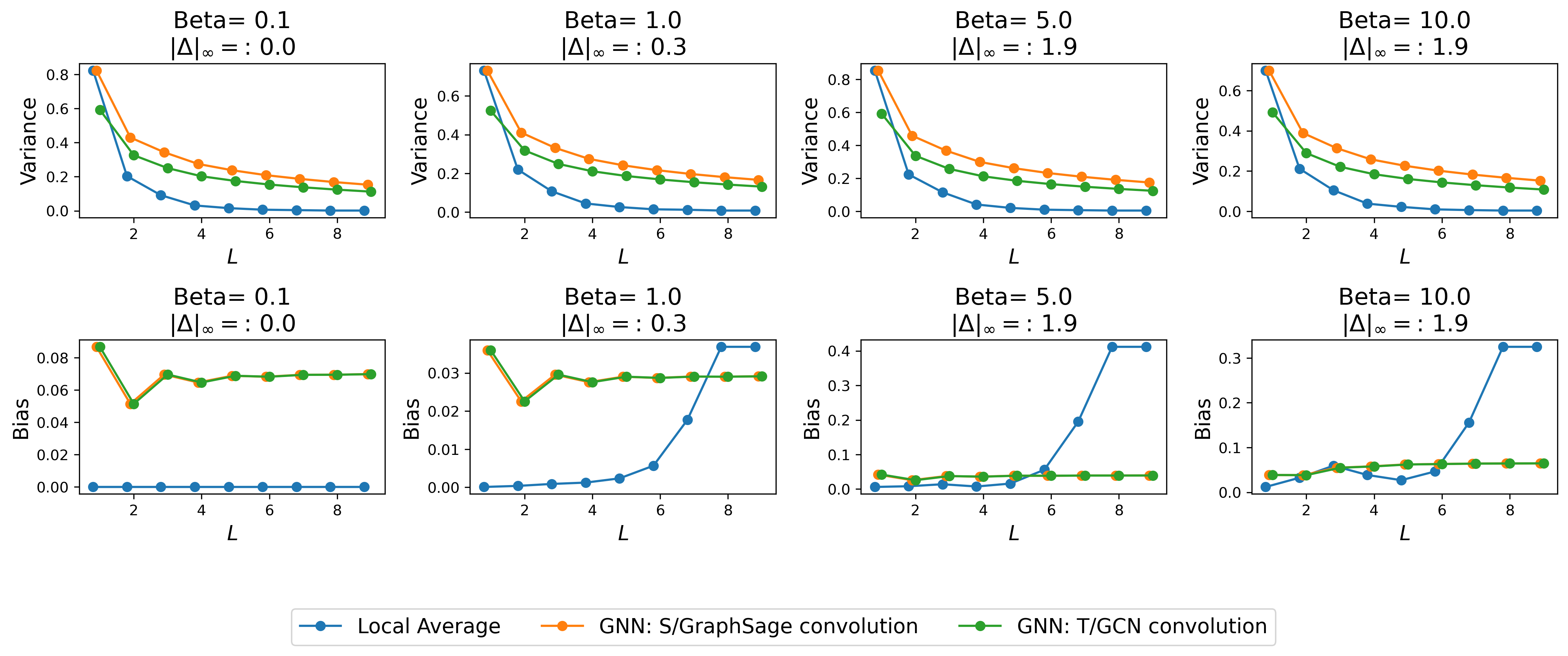
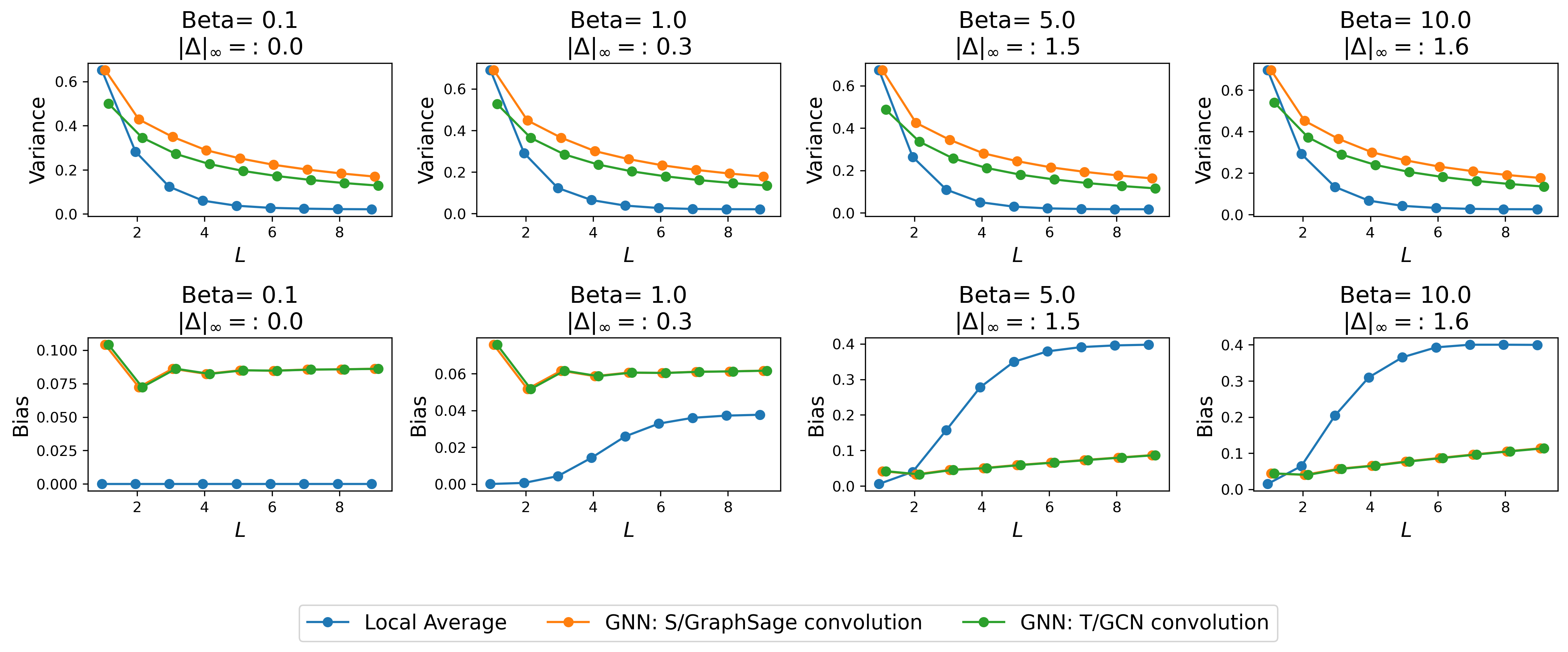
The next four sets of plots (Figures 11, 12, 13 and 14) highlight the bias-variance trade-off across different types of topologies. Overall, we observe a slower decay of the variance for the GraphSage convolution compared to the GCN convolution, for similar levels of bias.