Dynamic Kohn anomaly in twisted bilayer graphene

Abstract

Twisted bilayer graphene (TBG) has attracted great interest in the last decade due to the novel properties it exhibited. It was revealed that e-phonon interaction plays an important role in a variety of phenomena in this system, such as superconductivity and exotic phases. However, due to its complexity, the e-phonon interaction in TBG is not well studied yet. In this work, we study the electron interaction with the acoustic phonon mode in twisted bilayer graphene and one of its consequences, i.e., the Kohn anomaly. The Kohn anomaly in ordinary metals usually happens at phonon momentum $q=2k_{F}$ as a dramatic modification of the phonon frequency when the phonon wave vector nests the electron Fermi surface. However, novel Kohn anomaly can happen in topological semimetals, such as graphene and Weyl semimetals. In this work, we show that the novel dynamic Kohn anomaly can also take place in twisted bilayer graphene due to the nesting of two different Moire Dirac points by the phonon wave vector. Moreover, by tuning the twist angle, the dynamic Kohn anomaly in TBG shows different features. Particularly, at magic angle when the electron bandwidth is almost flat, the dynamic Kohn anomalies of acoustic phonons disappear. We also studied the effects of finite temperature and doping on the dynamic Kohn anomaly in TBG and discussed the experimental methods to observe the Kohn anomaly in such system.

I Introduction

Twisted bilayer graphene has intrigued great interest in recent years due to its fascinating properties, such as the unconventional superconductivity [1, 2, 3, 4, 5, 6, 7] at magic angle and the fractional quantum Hall effect at low magnetic field[10, 11, 12, 13, 8, 9]. Besides, the TBG can also exhibit a variety of exotic phases, such as the Chern insulator phase at integer fillings[14, 15, 16, 17, 18, 19, 20, 21, 22, 23] or the incommensurate Kekule pattern state[24, 25]. It was discovered that these exotic phases and properties are often related to the correlation effects originating from the interactions in the system. While the role of the e-e Coulomb interaction has been intensively studied in the Chern insulating state of the TBG[26, 27, 28, 29, 30, 31, 32, 33], the e-phonon interaction is relatively less studied due to the complexity of such interaction. On the other hand, it was revealed that the e-phonon interaction plays an important role in both the unconventional superconductivity in TBG[34, 35, 36, 37, 38, 39, 40, 42, 41] and some of the exotic state of the system, such as the Kekule spiral order phase[43].

A strict and complete study of all the phonon modes in the TBG is unrealistic due to the enormous number of the phonon modes in this system. Fortunately, only a small percentage of all the phonon modes couples strongly with the electrons and is important[35, 36, 37, 38, 39, 40, 41, 44, 45, 46]. Ref.[40] studied the nine dominant optical phonon modes in TBG and their effects on the electronic states of the system. In this work, we study the e-phonon interaction of the acoustic phonon modes which couple most strongly with the electrons in TBG, which is also considered to be the most important e-phonon coupling for the superconductivity in the TBG[35, 37].

We derive an effective e-phonon interaction Hamiltonian for the acoustic phonons interacting with electrons in the lowest two bands near the Fermi energy in the continuum model of the TBG. We then studied the dynamic Kohn anomaly [47, 48] in the system induced by the intervalley e-phonon scatterings. The dynamic Kohn anomaly in the continuum model TBG originates from the nesting of the Fermi surface near the Moire Dirac points by the phonon wavevector. Similar phenomena has been observed in 3D Weyl semimetal (WSM) TaP[49] and 2D graphene[50, 48, 51, 52]. However, we show that TBG exhibits different and more diverse behaviors of the Kohn anomaly due to the adjustable band structure by tuning the twisting angle. When the twist angle is away from the magic angle, the Kohn anomaly in TBG exhibits more similarity to that in Weyl semimetals. However, at magic angle when the two electron bands crossing the Fermi energy become almost flat, the Kohn anomaly induced by the acoustic phonon may disappear because the energy and momentum conservation cannot be satisfied at the same time in the e-phonon scattering processes in the system. The Kohn anomaly in TBG may be observed through inelastic x-ray[53] and neutron scatterings[54] in such system.

II Review of the Continuum model of the twisted bilayer graphene

We first have a brief review of the continuum model of TBG following Ref.[55, 56]. We consider a TBG with the two layers rotated by an angle $\theta/2$ and $-\theta/2$ respectively. Each single layer contains two sublattices labeled by $X=A,B$ in its unit cell. Without lattice distortion, the positions of sublattice $X$ on layer $l$ are given by

$$\mathbf{R}^{(l)}_{X}=m_{1}\mathbf{a}_{1}^{(l)}+m_{2}\mathbf{a}^{(l)}_{2}+\bm{\tau}^{(l)}_{X},$$ (1)

where $\mathbf{a}_{1}^{(l)}$ and $\mathbf{a}^{(l)}_{2}$ are the lattice unit vectors of graphene layer $l$, $m_{1},m_{2}$ are integers and $\bm{\tau}^{(l)}_{X}$ is the sublattice position of atom $X$ in the unit cell in layer $l$. For the unrotated graphene, $\bm{\tau}^{(l)}_{A}=(0,0),\bm{\tau}^{(l)}_{B}=a(0,-\sqrt{3}/3)$ with $a$ the bond length of graphene.

The Brillouin zones (BZ) of the single layer graphene and TBG are shown in Fig.1(a). The two Dirac points of the rotated single layer 1 and 2 are denoted as $\mathbf{K}^{(1)}_{\pm}$ and $\mathbf{K}^{(2)}_{\pm}$ respectively where $+$ and $-$ label the two valleys of a single graphene layer. The primitive reciprocal lattice vectors of layer $l$ are ${\mathbf{a}}^{*(l)}_{i}=R(\pm\theta/2){\mathbf{a}}^{*}_{i}$ for $l=1,2$ respectively, where ${\mathbf{a}}_{1}^{*}=(2\pi/a)(1,-1/\sqrt{3}),\mathbf{a}^{*}_{2}=(2\pi/a)(0,2/\sqrt{3})$ are the reciprocal lattice vectors for the unrotated graphene, and $R(\pm\theta/2)$ is the rotation operator. For a given valley, e.g., $\eta=+$, the Moire Reciprocal lattice vectors are given by $\textbf{g}_{\text{M}i}=\mathbf{a}^{*(1)}_{i}-\mathbf{a}_{i}^{*(2)},i=1,2,$ and the first Moire BZ of the TBG corresponds to the small hexagon in Fig.1a. We label the two Dirac points of the moire BZ for valley $+$ as $\mathbf{K}_{M1}$ and $\mathbf{K}_{M2}$.

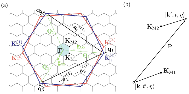
Figure 1: (a)Momentum-space geometry of the twisted bilayer graphene. The blue and red hexagons mark the first Brillouin zones of the rotated graphene layer 1 and 2 respectively. $\mathbf{K}^{(1)}_{\pm}$ and $\mathbf{K}^{(2)}_{\pm}$ label the Dirac points of the two rotated graphene layers and the subscripts $+$ and $-$ label the two valleys of a single graphene layer. The shaded hexagons represent the first Moire BZ of the superlattice. (b)Schematic description of an electron scattering from state $|\mathbf{k},t^{\prime},\eta\rangle$ to $|\mathbf{k}^{\prime},t,\eta\rangle$ by a phonon with momentum $\mathbf{p}$, where $t,t^{\prime}=\pm$ are the band indices.

The electronic band structure of the TBG has been studied extensively in previous works[55, 56, 58, 60, 59, 57]. We employ the continuum model in Ref.[55, 56] to describe the low energy electronic structure of the TBG in this work. In such model, the hopping processes from the valley $+$ to $-$ between the two layers are neglected due to the large momentum transfer. For valley $\pm$, only the three dominant hopping processes near the Dirac points of the two layers with momentum transfer $0$, $\mp{\mathbf{g}}_{M1}$ and $\mp{\mathbf{g}}_{M1}\mp{\mathbf{g}}_{M2}$ between the two layers are retained. The low energy Hamiltonian of the TBG at valley $\eta$ is then described by the Dirac spinor fields $\psi^{(1)}_{\eta}$ and $\psi^{(2)}_{\eta}$ of layer $1$ and layer $2$ as:

$$H_{0,\eta}=\sum_{\eta}\int d\mathbf{r}\left(\psi^{(1)\dagger}_{\eta},\,\psi^{(2)\dagger}_{\eta}\right)\begin{pmatrix}\hbar v_{F}(-i{\bm{\nabla}}-\mathbf{K}^{(1)}_{\eta})\cdot{\bm{\sigma}}_{\theta/2}&\hat{T}(\mathbf{r})\\ \hat{T}^{\dagger}(\mathbf{r})&\hbar v_{F}(-i{\bm{\nabla}}-\mathbf{K}^{(2)}_{\eta})\cdot{\bm{\sigma}}_{-\theta/2}\end{pmatrix}\begin{pmatrix}\psi^{(1)}_{\eta}\\ \psi^{(2)}_{\eta}\end{pmatrix}.$$ (2)

Here the diagonal matrix elements describe the Hamiltonian of the rotated single layer 1 and 2 near the Dirac points and $\bm{\sigma}_{\theta/2}=e^{\pm i\theta\sigma_{z}/4}(\eta\sigma_{x},-\sigma_{y})e^{\mp i\theta\sigma_{z}/4}$. For small rotation angle $\theta$, $e^{\pm i\theta\sigma_{z}/4}\approx 1$ and the rotation factor for the single layers can be neglected.

The off-diagonal matrices $\hat{T}(\mathbf{r})$ and $\hat{T}^{\dagger}(\mathbf{r})$ describe the hopping processes between the two layers. In the continuum model, it is assumed that the interlayer tunneling amplitude between the carbon $p_{z}$ orbital is a smooth function $T(\mathbf{r})$ of the spatial separation projected onto the graphene planes. The tunneling matrix element for an electron with momentum $\mathbf{k}$ on the sublattice $X$ in layer 1 to layer 2 with momentum $\mathbf{k}^{\prime}$ on sublattice $X^{\prime}$ is

$$T_{\mathbf{k}X}^{\mathbf{k}^{\prime}X^{\prime}}=\bra{\mathbf{k}^{\prime},X^{\prime},2}U\ket{\mathbf{k},X,1},$$ (3)

where the Bloch states in a single-layer $l$ can be written as

$$\ket{\mathbf{k},X,l}=\frac{1}{\sqrt{N}}\sum_{\mathbf{R}\in\mathbf{R}_{X}^{(l)}}e^{i\mathbf{k}\cdot\mathbf{R}}\ket{\mathbf{R}+\mathbf{u}^{(l)}_{X}+h^{(l)}_{X}\mathbf{z}}$$ (4)

with $\mathbf{u}^{(l)}_{X}$ and $h^{(l)}_{X}\mathbf{z}$ the atomic displacement parallel and perpendicular to the graphene plane respectively. The interlayer hopping matrix element then becomes

$$\bra{\mathbf{k}^{\prime},X^{\prime},2}U\ket{\mathbf{k},X,1}=-\frac{1}{N}\sum_{\mathbf{R}^{\prime}\in\mathbf{R}_{X^{\prime}}^{(2)}}\sum_{\mathbf{R}\in\mathbf{R}_{X}^{(1)}}e^{i\mathbf{k}\cdot\mathbf{R}-i\mathbf{k}^{\prime}\cdot\mathbf{R}^{\prime}}T\left(\mathbf{R}^{\prime}+\mathbf{u}^{(2)}_{X^{\prime}}+h^{(2)}_{X^{\prime}}\mathbf{z}-\mathbf{R}-\mathbf{u}^{(1)}_{X}-h^{(1)}_{X}\mathbf{z}\right),$$ (5)

where

$$T\left(\mathbf{R}^{\prime}+\mathbf{u}^{(2)}_{X^{\prime}}+h^{(2)}_{X^{\prime}}\mathbf{z}-\mathbf{R}-\mathbf{u}^{(1)}_{X}-h^{(1)}_{X}\mathbf{z}\right)=-\bra{\mathbf{R}^{\prime}+\mathbf{u}^{(2)}_{X^{\prime}}+h^{(2)}_{X^{\prime}}\mathbf{z}}U\ket{\mathbf{R}+\mathbf{u}^{(1)}_{X}+h^{(1)}_{X}\mathbf{z}}$$ (6)

only depends on the distance of the two carbon atoms.

At zero atomic displacement, i.e., $\mathbf{u}^{(l)}_{X}=0,\mathbf{h}^{(l)}_{X}=0$, one can perform the Fourier transform of $T(\mathbf{r})$ in Eq.(5) followed by the sum over the lattice sites $\mathbf{R}$ and $\mathbf{R}^{\prime}$ and get

$$T_{\mathbf{k}X}^{\mathbf{k}^{\prime}X^{\prime}}=-\sum_{\mathbf{G}^{(1)},\mathbf{G}^{(2)}}T_{\parallel}(\mathbf{k}+\mathbf{G}^{(1)},d_{X^{\prime}X})e^{-i[\mathbf{G}^{(1)}\cdot{\bm{\tau}}^{(1)}_{X}-\mathbf{G}^{(2)}\cdot\bm{\tau}^{(2)}_{X^{\prime}}]}\delta_{\mathbf{k}+\mathbf{G}^{(1)},\mathbf{k}^{\prime}+\mathbf{G}^{(2)}}$$ (7)

where $\mathbf{G}^{(1)},\mathbf{G}^{(2)}$ are reciprocal lattice vectors for layer 1 and layer 2, $d_{X^{\prime}X}$ is the $z$ direction distance between the nearest $X$ and $X^{\prime}$ atom in the two layers and

$$T_{\parallel}(\mathbf{Q},z)=\frac{d_{0}}{2\pi}\int dp_{z}T_{\mathbf{Q}+p_{z}\hat{\mathbf{z}}}e^{ip_{z}z}=\frac{1}{S_{0}}\int d^{2}re^{-i\mathbf{Q}\cdot\mathbf{r}}T\left(\mathbf{r}+d\hat{\mathbf{z}}\right)$$ (8)

is the Fourier transform of the hopping matrix in terms of the in-plane coordinates with $T_{\mathbf{Q}+p_{z}\hat{\mathbf{z}}}$ the 3D Fourier transform of $T(\mathbf{r})$ and $S_{0}$ the unit cell area.

Since $T_{\parallel}(\mathbf{Q},d_{XX^{\prime}})$ decays quickly with large $Q$, for $\mathbf{k}$ near the Dirac point $\mathbf{K}^{(1)}_{+}$ and $\mathbf{k}^{\prime}$ near the Dirac point $\mathbf{K}^{(2)}_{+}$, the dominant coupling occurs in three cases $(\mathbf{G}^{(1)},\mathbf{G}^{(2)})=(0,0),(-\mathbf{a}^{*(1)}_{1},-\mathbf{a}^{*(2)}_{1}),(-\mathbf{a}^{*(1)}_{1}-\mathbf{a}^{*(1)}_{2},-\mathbf{a}^{*(2)}_{1}-\mathbf{a}^{*(2)}_{2})$. The corresponding $\mathbf{Q}_{j}\equiv\mathbf{k}+\mathbf{G}^{(1)}$ is close to the three equivalent Dirac points of the first BZ of the non-rotated graphene layer $1$. In the continuum model, only these three components of $T_{\parallel}(\mathbf{Q}_{j},d_{XX^{\prime}})$ are retained and the matrix elements $T^{\mathbf{k}^{\prime}}_{\mathbf{k}^{\prime}}$ in Eq.(7) corresponding to these three processes in the sublattice basis are

$$\begin{gathered}T_{1}=\begin{pmatrix}t_{0}&t_{1}\\ t_{1}&t_{0}\end{pmatrix},\,T_{2}=\begin{pmatrix}t_{0}&t_{1}e^{i\frac{2\pi}{3}}\\ t_{1}e^{-i\frac{2\pi}{3}}&t_{0}\end{pmatrix},T_{3}=\begin{pmatrix}t_{0}&t_{1}e^{-i\frac{2\pi}{3}}\\ t_{1}e^{i\frac{2\pi}{3}}&t_{0}\end{pmatrix},\end{gathered}$$ (9)

where $t_{0}=-T_{\parallel}(\mathbf{Q}_{j},d_{AA}),t_{1}=-T_{\parallel}(\mathbf{Q}_{j},d_{AB})$. Due to the lattice relaxation, the interlayer distance of the AA region becomes greater than the AB region, i.e.,, $d_{AA}>d_{AB}$. For the reason, the hopping energy $t_{0}$ is smaller than $t_{1}$. In Ref.[60], the hopping integral $t_{1}$ is estimated to be $110\rm meV$ and $t_{0}\approx 0.8t_{1}$.

The electronic Hamiltonian for valley $+$ keeping only the three $T^{i}$ matrices is [55]

$$H_{0,\eta=+}=\int d\mathbf{r}\left(\psi^{{\dagger}(1)}_{\eta=+},\,\psi^{{\dagger}(2)}_{\eta=+}\right)\begin{pmatrix}\hbar v_{F}(-i{\bm{\nabla}}-\mathbf{K}^{(1)}_{+})\cdot(\sigma_{x},-\sigma_{y}),&\sum_{j=1}^{3}(T_{j})^{\dagger}e^{-i\delta\mathbf{k}_{j}\cdot\mathbf{r}}\\ \sum_{j=1}^{3}T_{j}e^{i\delta\mathbf{k}_{j}\cdot\mathbf{r}},&\hbar v_{F}(-i{\bm{\nabla}}-\mathbf{K}^{(2)}_{+})\cdot(\sigma_{x},-\sigma_{y})\end{pmatrix}\begin{pmatrix}\psi^{(1)}_{\eta=+}\\ \psi^{(2)}_{\eta=+}\end{pmatrix},$$ (10)

where $\delta\mathbf{k}_{j}=0,-\mathbf{g}_{M_{1}},-\mathbf{g}_{M_{1}}-\mathbf{g}_{M_{2}}$ for $j=1,2,3$ respectively and is equal to the momentum transfers between the two layers for the hopping processes.

The Hamiltonian in the momentum space can be truncated using the four single-layer spinor states involved in the three dominant hopping processes, i.e., $|\mathbf{k},1\rangle$ and $|\mathbf{k}^{\prime}=\mathbf{k}+\delta\mathbf{k}_{i},2\rangle,i=1,2,3$ as basis, and one gets the truncated Hamiltonian for valley $+$ as [56, 58]

$$H_{\eta=+,\mathbf{K}_{M1}}^{8\times 8}(\mathbf{k})=\begin{pmatrix}v_{F}(\mathbf{k}-\mathbf{K}^{(1)}_{+})\cdot\bm{\sigma}^{*}&T_{1}^{\dagger}&T_{2}^{\dagger}&T_{3}^{\dagger}\\ T_{1}&v_{F}(\mathbf{k}+\delta\mathbf{k}_{1}-\mathbf{K}^{(2)}_{+})\cdot\bm{\sigma}^{*}&0&0\\ T_{2}&0&v_{F}(\mathbf{k}+\delta\mathbf{k}_{2}-\mathbf{K}^{(2)}_{+})\cdot\bm{\sigma}^{*}&0\\ T_{3}&0&0&v_{F}(\mathbf{k}+\delta\mathbf{k}_{3}-\mathbf{K}^{(2)}_{+})\cdot\bm{\sigma}^{*}\end{pmatrix},$$ (11)

where $\bm{\sigma}^{*}=(\sigma_{x},-\sigma_{y})$ acts on the sublattice basis.

The Moire momentum $\tilde{\mathbf{k}}$ characterizing the band structure of the TBG can be obtained by zone folding of the single layer momentum $\mathbf{k}$ or $\mathbf{k}^{\prime}$ to the Moire BZ, i.e., $\mathbf{k}=\tilde{\mathbf{k}}+m_{1}\mathbf{g}_{M1}+m_{2}\mathbf{g}_{M2},\mathbf{k}^{\prime}=\tilde{\mathbf{k}}+n_{1}\mathbf{g}_{M1}+n_{2}\mathbf{g}_{M2}$, where $m_{1},m_{2},n_{1},n_{2}$ are integers and $\tilde{\mathbf{k}}$ locates in the Moire BZ. The Hamiltonian Eq.(11) gives eight effective low energy bands for the TBG. There are two bands per spin and per valley in the middle of the spectrum that touch at two inequivalent Moire Dirac points $\mathbf{K}_{M1}$ and $\mathbf{K}_{M2}$ shown in Fig.1(a) with a linear dispersion due to the $\hat{\mathcal{C}}_{2z}\hat{\mathcal{T}}$ and $\hat{\mathcal{C}}_{3z}$ symmetry[34]. At neutrality, the Fermi energy locates at the Moire Dirac points. An effective $2*2$ Hamiltonian for the two bands near the Moire Dirac point $\mathbf{K}_{M1}$ was constructed by the $\mathbf{k}\cdot\mathbf{p}$ expansion near $\mathbf{K}_{M1}$ as[56, 58]

$$H^{*}(\tilde{\mathbf{k}})=\hbar v(\tilde{\mathbf{k}}-\mathbf{K}_{M1})\cdot\bm{\sigma}^{*}$$ (12)

where $v=\frac{1-3\alpha_{1}^{2}}{1+3\alpha_{0}^{2}+3\alpha_{1}^{2}}v_{F}$ with $\alpha_{0}=\frac{t_{0}}{\hbar v_{F}\absolutevalue{\mathbf{q}_{1}}},\alpha_{1}=\frac{t_{1}}{\hbar v_{F}\absolutevalue{\mathbf{q}_{1}}}$. The effective Hamiltonian near ${\mathbf{K}}_{M2}$ has the same form by replacing ${\mathbf{K}}_{M1}$ by ${\mathbf{K}}_{M2}$. The two Moire Dirac points $\mathbf{K}_{M1}$ and $\mathbf{K}_{M2}$ carry the same chirality[61, 62, 63] because they originate from the unperturbed Dirac cones of the two different layers in the same valley.

III Electron-phonon interaction Hamiltonian in the TBG

TBG contains a large number of phonon modes due to the large number of atoms in a unit cell. However, only a limited number of phonon modes couple strongly with the electrons. Ref.[40] studied the nine dominant optical phonon modes which couple strongly with the electrons and their effects on stablizing the electron order in the system. In this work, we instead focus on the most important acoustic mode, i.e., the in-plane $\mathbf{u}^{-}$ mode in TBG in the following text, which was considered to be the dominant phonon mode resulting in the superconductivity in TBG[35].

III.1 Interlayer e-phonon scattering matrix

The interlayer electron-phonon interaction Hamiltonian in TBG can be obtained by expanding the hopping matrix elements in Eq.(5) in terms of the lattice displacement $\mathbf{u}_{X}^{(l)}$ and $h_{X}^{(l)}$, as shown in Ref.[64, 65]. Since the flexural mode $h_{X}^{(l)}$ perpendicular to the graphene plane has quadratic dispersion[66] and is weak at low energy. We only consider the in-plane mode $\mathbf{u}_{X}^{(l)}$ in the following. We absorb the static lattice relaxation effects to the hopping integral $t_{0}$ and $t_{1}$ and only consider the expansion in terms of the dynamic vibration of the lattice. It was shown that the static lattice relaxation does not change the electronic band structure qualitatively [64].

Since the interlayer hopping energy only depends on the relative displacement of the two layers, i.e., $\mathbf{u}^{-}=\mathbf{u}^{(2)}-\mathbf{u}^{(1)}$, we only consider the dominant acoustic phonon modes corresponding to $\mathbf{u}^{-}$ and neglect the centre of mass modes $\mathbf{u}^{+}=(\mathbf{u}^{(2)}+\mathbf{u}^{(1)})/2$.

At finite displacement $\mathbf{u}^{(l)}_{X}$, the interlayer hopping matrix element Eq.(5) after the Fourier transform of $T({\mathbf{r}})$ becomes

$$\bra{\mathbf{k}^{\prime},X^{\prime},2}U\ket{\mathbf{k},X,1}=-\frac{1}{N}\frac{S_{0}d_{0}}{(2\pi)^{3}}\int d^{3}\tilde{\mathbf{p}}T(\tilde{\mathbf{p}})\sum_{\mathbf{R}\in\mathbf{R}^{(1)}_{X},\mathbf{R}^{\prime}\in\mathbf{R}^{(2)}_{X^{\prime}}}e^{i(\mathbf{k}-\tilde{\mathbf{p}})\mathbf{R}-i\tilde{\mathbf{p}}\cdot\mathbf{u}^{(1)}_{X}(\mathbf{R})}e^{-i(\mathbf{k}^{\prime}-\tilde{\mathbf{p}})\mathbf{R}^{\prime}+i\tilde{\mathbf{p}}\cdot\mathbf{u}^{(2)}_{X^{\prime}}(\mathbf{R}^{\prime})}.$$ (13)

Following the procedure in Ref.[64], i.e., replacing $u^{(l)}_{X}$ by its Fourier transform

$$\mathbf{u}_{X}^{(l)}(\mathbf{r})=\frac{1}{\sqrt{S}}\sum_{\mathbf{p}}\mathbf{u}_{X,\mathbf{p}}^{(l)}e^{i\mathbf{p}\cdot\mathbf{r}},\quad$$ (14)

and expanding the exponential functions $\exp(i\tilde{\mathbf{p}}\cdot\mathbf{u}_{\mathbf{p}}e^{i\mathbf{p}\cdot\mathbf{R}})$ in a Taylor series, one gets the interlayer hopping matrix element after the sum over the lattice sites $\mathbf{R}$ and $\mathbf{R}^{\prime}$ as

$$\bra{\mathbf{k}^{\prime},X^{\prime},2}U\ket{\mathbf{k},X,1}$$ (15)

$$= \sum_{\mathbf{G}^{(1)},\mathbf{G}^{(2)}}\sum_{n_{1},n_{2},..}\sum_{n^{\prime}_{1},n^{\prime}_{2},..}\Gamma^{(n^{\prime}_{1},n^{\prime}_{2}..)}_{(n_{1},n_{2},..)}(\mathbf{Q})e^{-i(\mathbf{G}^{(1)}\cdot\bm{\tau}^{(1)}_{X}-\mathbf{G}^{(2)}\cdot\bm{\tau}^{(2)}_{X^{\prime}})}\delta_{\mathbf{k}+\mathbf{G}^{(1)}+n_{1}\mathbf{p}_{1}..,\ \mathbf{k}^{\prime}+\mathbf{G}^{(2)}-n^{\prime}_{1}\mathbf{p}_{1}-..}$$

where $\mathbf{p}_{1,2}$ are the momentum from the Fourier transform of $\mathbf{u}^{(l)}_{X}$, and $\mathbf{Q}=\mathbf{k}+\mathbf{G}^{(1)}+n_{1}\mathbf{p}_{1}+n_{2}\mathbf{p}_{2}+..=\mathbf{k}^{\prime}+\mathbf{G}^{(2)}-n^{\prime}_{1}\mathbf{p}_{1}-n^{\prime}_{2}\mathbf{p}_{2}-..$, with $n_{i},n^{\prime}_{i}=0,1,2...$. The Fourier component of the hopping matrix

$$\Gamma^{(n^{\prime}_{1},n^{\prime}_{2},..)}_{(n_{1},n_{2},..)}(\mathbf{Q})= -\frac{d_{0}}{2\pi}\int dp_{z}\,T_{\mathbf{Q}+p_{z}\hat{\mathbf{z}}}e^{ip_{z}d_{X^{\prime}X}}\frac{\left[-i\mathbf{Q}\cdot\mathbf{u}^{(1)}_{X,\mathbf{p}_{1}}\right]^{n_{1}}}{n_{1}!(\sqrt{S})^{n_{1}}}\frac{\left[-i\mathbf{Q}\cdot\mathbf{u}^{(1)}_{X,\mathbf{p}_{2}}\right]^{n_{2}}}{n_{2}!(\sqrt{S})^{n_{2}}}...\frac{\left[i\mathbf{Q}\cdot\mathbf{u}^{(2)}_{X^{\prime},\mathbf{p}_{1}}\right]^{n^{\prime}_{1}}}{n^{\prime}_{1}!(\sqrt{S})^{n^{\prime}_{1}}}\frac{\left[i\mathbf{Q}\cdot\mathbf{u}^{(2)}_{X^{\prime},\mathbf{p}_{2}}\right]^{n^{\prime}_{2}}}{n^{\prime}_{2}!(\sqrt{S})^{n^{\prime}_{2}}}...$$ (16)

For small twist angles and long range displacement, $u^{(l)}_{A}(\mathbf{r})\approx u^{(l)}_{B}(\mathbf{r})=u^{(l)}(\mathbf{r})$, where $u^{(l)}(\mathbf{r})$ is smooth varying compared to the atomic scale, $\mathbf{p}$ in $\mathbf{u}^{(l)}_{\mathbf{p}}$ is much smaller than $1/a$ and one can neglect the small shift $n_{1}\mathbf{p}_{1}+n_{2}\mathbf{p}_{2}+...$ in $\mathbf{Q}$ in the coupling amplitude $\Gamma^{(n^{\prime}_{1},n^{\prime}_{2},..)}_{(n_{1},n_{2},..)}(\mathbf{Q})$ and replace $\mathbf{Q}$ by the three ${\mathbf{Q}}_{j}$ in the above text, i.e., $\mathbf{Q}_{1}=\mathbf{K}_{+},\ \mathbf{Q}_{2}=\mathbf{K}_{+}-\mathbf{a}^{*}_{1},\ \mathbf{Q}_{3}=\mathbf{K}_{+}-\mathbf{a}^{*}_{1}-\mathbf{a}^{*}_{2}.$ In the leading order we only need to keep the linear order of the displacement $\mathbf{u}_{\mathbf{p}}$ and get the e-phonon interaction matrix element as

$$\bra{\mathbf{k}^{\prime},X^{\prime},2}H_{e-ph}\ket{\mathbf{k},X,1}$$ (17)

$$= -\frac{1}{\sqrt{S}}\sum_{\mathbf{p}}\sum_{j=1,2,3}T_{\parallel}\left(\mathbf{Q}_{j};\,d_{X^{\prime}X}\right)e^{i(-\mathbf{G}_{j}^{(1)}\cdot\bm{\tau}^{(1)}_{X}+\mathbf{G}_{j}^{(2)}\cdot\bm{\tau}^{(2)}_{X^{\prime}})}\left(i\mathbf{Q}_{j}\cdot\mathbf{u}^{-}_{\mathbf{p}}\right)\delta_{\mathbf{k}+\delta\mathbf{k}_{j}+\mathbf{p},\mathbf{k}^{\prime}},$$

where $\mathbf{u}^{-}_{\mathbf{p}}$ is the Fourier transform of $\mathbf{u}^{-}(\mathbf{r})$. This matrix element can be written in the sublattice basis as

$$\bra{\mathbf{k}^{\prime},2}H_{e-ph}\ket{\mathbf{k},1}=\frac{1}{\sqrt{S}}\sum_{\mathbf{p}}\sum_{j=1,2,3}T_{j}\left(i\mathbf{Q}_{j}\cdot\mathbf{u}^{-}_{\mathbf{p}}\right)\delta_{\mathbf{k}+\delta\mathbf{k}_{j}+\mathbf{p},\mathbf{k}^{\prime}},$$ (18)

where $T_{i},i=1,2,3$ is defined in the last section.

III.2 Intra-layer e-phonon scattering matrix

For e-phonon scatterings within the same single-layer, we neglect the weak interaction between the two layers, and the electron-phonon Hamiltonian is identical to that in single-layer graphene. In the continuum limit, the matrix element is given by[67, 68, 69]

$$\bra{\mathbf{k}^{\prime},l}H_{e-ph}\ket{\mathbf{k},l}=ev_{F}\left(\sum_{\mathbf{p}}\mathbf{A}^{(l)}_{\eta,\mathbf{p}}\delta_{\mathbf{k}^{\prime},\mathbf{k}+\mathbf{p}}\right)\cdot(\eta\sigma_{x},-\sigma_{y}),$$ (19)

where $\mathbf{A}^{(l)}_{\eta}$ represents the pseudo-vector potential resulting from in-plane lattice displacement. The out-of-plane single layer phonon mode couples quadratically to the electrons[70, 71] and does not contribute to the intra-layer e-phonon scattering in the first-order so we neglect it. The single layer pseudo-vector potential is expressed as[67, 68, 69]

$$\mathbf{A}^{(l)}_{\eta,\mathbf{p}}=-\frac{3}{4}\eta\frac{\beta_{0}\gamma_{0}}{ev_{F}}(\hat{W}_{\mathbf{p}}\,\mathbf{u}^{(l)}_{\mathbf{p}}).$$ (20)

Furthermore, $\beta_{0}\approx 3.14$ remains constant[64], and $\gamma_{0}=2.8\,\text{eV}$ represents the electronic nearest hopping energy in single-layer graphene. The matrix $\hat{W}_{\mathbf{p}}$ is given by[67, 68, 69]

$$\hat{W}_{\mathbf{p}}=\matrixquantity(ip_{x}&-ip_{y}\\ -ip_{y}&-ip_{x})$$ (21)

The in-plane phonon modes can be divided into the longitudinal mode with polarization direction $\hat{\mathbf{e}}_{\mathbf{p},L}=\mathbf{p}/|\mathbf{p}|$ and transverse mode with polarization direction $\hat{\mathbf{e}}_{\mathbf{p},T}=\hat{\mathbf{e}}_{z}\crossproduct\mathbf{p}/|\mathbf{p}|$. The atomic displacement can then be quantized as[35]

$$\mathbf{u}^{-}_{\mathbf{p}} = \sum_{\chi=T,L}\sqrt{\frac{\hbar}{\rho\omega_{0,\mathbf{p},\chi}}}i\hat{\mathbf{e}}_{\mathbf{p},\chi}\left(\hat{a}_{\mathbf{p},\chi}+\hat{a}^{\dagger}_{-\mathbf{p},\chi}\right),$$ (22)

where $\hat{a}_{\mathbf{p},\chi}$ is the in-plane phonon annihilation operator with momentum $\mathbf{p}$ and polarization $\chi=L,T$. The phonon frequency $\omega_{0,\mathbf{p},\chi}=c_{\chi}|\mathbf{p}|$ for $\chi=L,T$. For simplicity[67, 35], we take $c_{L}=c_{T}=s=10^{4}\text{ m/s}$.

III.3 Projection of e-phonon interaction to the lowest two bands

At low energy, we only need to consider the two bands near $E=0$. The effective Hamiltonian for this two-band system is given in Eq.(12) in the sub-lattice basis. The two eigenstates of the two-band system near the Moire Dirac point ${\mathbf{K}}_{M1}$ can be solved as

$$\ket{\bm{\phi}^{s=+}_{\eta=+}(\tilde{\mathbf{k}})} = \frac{1}{\sqrt{1+3\alpha_{0}^{2}+3\alpha_{1}^{2}}}\left[\ket{\mathbf{k},A,1}-\sum_{j=1,2,3}\left(-i\alpha_{1}\ket{\mathbf{k}+\delta\mathbf{k}_{j},A,2}+i\alpha_{0}e^{-i\frac{2\pi}{3}(j-1)}\ket{\mathbf{k}+\delta\mathbf{k}_{j},B,2}\right)\right],$$ (23)

$$\ket{\bm{\phi}^{s=-}_{\eta=+}(\tilde{\mathbf{k}})} = \frac{1}{\sqrt{1+3\alpha_{0}^{2}+3\alpha_{1}^{2}}}\left[\ket{\mathbf{k},B,1}-\sum_{j=1,2,3}\left(-i\alpha_{0}e^{i\frac{2\pi}{3}(j-1)}\ket{\mathbf{k}+\delta\mathbf{k}_{j},A,2}+i\alpha_{1}\ket{\mathbf{k}+\delta\mathbf{k}_{j},B,2}\right)\right].$$ (24)

Similarly, the eigenstates near the Moire Dirac point ${\mathbf{K}}_{M2}$ are solved as

$$\bra{\bm{\phi}^{s^{\prime}=+}_{\eta=+}(\tilde{\mathbf{k}}^{\prime})} = \frac{1}{\sqrt{1+3\alpha_{0}^{2}+3\alpha_{1}^{2}}}\left[\bra{\mathbf{k}^{\prime},A,2}+\sum_{m=1,2,3}\left(i\alpha_{1}\bra{\mathbf{k}^{\prime}-\delta\mathbf{k}_{m},A,1}-i\alpha_{0}e^{i\frac{2\pi}{3}(m-1)}\bra{\mathbf{k}^{\prime}-\delta\mathbf{k}_{m},B,1}\right)\right],$$ (25)

$$\bra{\bm{\phi}^{s^{\prime}=-}_{\eta=+}(\tilde{\mathbf{k}}^{\prime})} = \frac{1}{\sqrt{1+3\alpha_{0}^{2}+3\alpha_{1}^{2}}}\left[\bra{\mathbf{k}^{\prime},B,2}+\sum_{m=1,2,3}\left(i\alpha_{0}e^{-i\frac{2\pi}{3}(m-1)}\bra{\mathbf{k}^{\prime}-\delta\mathbf{k}_{m},A,1}-i\alpha_{1}\bra{\mathbf{k}^{\prime}-\delta\mathbf{k}_{m},B,1}\right)\right]$$ (26)

where $\mathbf{k},\mathbf{k}^{\prime}$ are the single layer momentum near $\mathbf{K}^{(1)}_{+}$ and $\mathbf{K}^{(2)}_{+}$ respectively, and $\tilde{\mathbf{k}},\tilde{\mathbf{k}^{\prime}}$ are the Moire momentum band-folded from the single layer momentum $\mathbf{k}$ and $\mathbf{k}^{\prime}$. At $\mathbf{k}=\mathbf{K}^{(1)}_{+}$, i.e., $\tilde{\mathbf{k}}=\mathbf{K}_{M1}$, $|\phi^{\pm}_{+}(\tilde{\mathbf{k}})\rangle$ give the two degenerate eigenstates of Eq.(11) with $E=0$. Similarly, at $\mathbf{k}^{\prime}=\mathbf{K}^{(2)}_{+}$, i.e., $\tilde{\mathbf{k}}^{\prime}=\mathbf{K}_{M2}$, $|\phi^{\pm}_{+}(\tilde{\mathbf{k}^{\prime}})\rangle$ give the two degenerate eigenstates with $E=0$ at $\mathbf{K}_{M2}$.

At zero doping, the Fermi surface aligns with the Moire Dirac points $\mathbf{K}_{\text{M1}}$ and $\mathbf{K}_{\text{M2}}$ of the two bands crossing $E=0$. We then focus on the inter-Moire-Dirac-point scatterings induced by phonons, which may result in a dynamic Kohn anomaly due to the nesting of the Fermi surface. Considering the e-phonon scatterings in the valley $+$, the scattering matrix from the two eigenstates $|\phi^{\pm}_{+}(\tilde{\mathbf{k}})\rangle$ near $\mathbf{K}_{M1}$ to the two eigenstates $|\phi^{\pm}_{+}(\tilde{\mathbf{k}}^{\prime})\rangle$ near $\mathbf{K}_{M2}$ can be obtained from Eq.(18), (19), (23)-(26) and written in the sublattice basis as

$$\bra{\bm{\phi}^{s^{\prime}}_{+}(\tilde{\mathbf{k}}^{\prime})}H_{e-ph}\ket{\bm{\phi}^{s}_{+}(\tilde{\mathbf{k}})}=\frac{1}{\sqrt{S}}\sum_{\chi}\sum_{\mathbf{p}}[\hat{g}_{+,\chi}(\mathbf{p})]_{s^{\prime}s}\delta_{\tilde{\mathbf{k}}^{\prime},\tilde{\mathbf{k}}+\mathbf{p}+m\mathbf{g}_{\mathbf{M}1}+n\mathbf{g}_{\mathbf{M}2}}(a_{\mathbf{p},\chi}+a^{\dagger}_{-\mathbf{p},\chi}),$$ (27)

where $\tilde{\mathbf{k}^{\prime}}$ and $\tilde{\mathbf{k}}$ are the Moire momentum near $\mathbf{K}_{M1}$ and $\mathbf{K}_{M2}$ respectively, $\mathbf{p}$ is the phonon momentum and the $\delta$ function gives the momentum conservation during the e-phonon scatterings. The Umklapp processes are subleading due to the large mismatch of energy and momentum so we only consider the case $m=0,n=0$.

For $\tilde{\mathbf{k}}(\tilde{\mathbf{k}}^{\prime})$ locating near $\mathbf{K}_{M1}(\mathbf{K}_{M2})$ or its two other equivalent Moire Dirac points, the phonon momenta for the inter-Moire-Dirac-point scattering then take the values $\mathbf{p}\approx-\mathbf{q}_{m},m=1,2,3$. The scattering matrices with these three phonon momenta are connected by the ${\cal C}_{3z}$ symmetry. The scattering matrix $\hat{g}_{+,\chi}(\mathbf{p})$ includes the contribution from both inter-layer and intra-layer scatterings, i.e., $\hat{g}_{+,\chi}(\mathbf{p})=\hat{g}^{\rm inter}_{+,\chi}(\mathbf{p})+\hat{g}^{\rm intra}_{+,\chi}(\mathbf{p})$. For $\mathbf{p}\approx-\mathbf{q}_{1}$, we get the interlayer scattering matrix in the sublattice basis as

$$\hat{g}^{\rm inter}_{\eta=+,\chi=T,L}(\mathbf{p})=$$

$$-\xi\sqrt{\frac{\hbar}{\rho\omega_{0,\mathbf{p},\chi}}}\left[\hat{T}_{1}(\mathbf{Q}_{1}\cdot\hat{\mathbf{e}}_{\mathbf{p},\chi})-\sum_{i,j,n=1,2,3}\left(\frac{\hat{T}_{i}^{\dagger}}{\hbar v_{F}\absolutevalue{\mathbf{q}_{1}}}\right)\left(\frac{\mathbf{q}_{i}\cdot\bm{\sigma}^{*\dagger}}{\absolutevalue{\mathbf{q}_{1}}}\right)\hat{T}_{n}\left(\frac{-\mathbf{q}_{j}\cdot\bm{\sigma}^{*}}{\absolutevalue{\mathbf{q}_{1}}}\right)\left(\frac{\hat{T}_{j}}{\hbar v_{F}\absolutevalue{\mathbf{q}_{1}}}\right)(\mathbf{Q}_{n}\cdot\hat{\mathbf{e}}_{\mathbf{p},\chi})\right],$$ (28)

where $\chi=T,L$ represent the transverse and longitudinal phonon modes respectively, $\bm{\sigma}^{*}$ acts on the sublattice basis, $\xi=\frac{1}{1+3\alpha_{0}^{2}+3\alpha_{1}^{2}}$ and ${\hat{\mathbf{e}}}_{\mathbf{p},\chi}$ is the polarization direction of the phonon modes. For $\mathbf{p}\approx-\mathbf{q}_{1}$, the momentum conservation restricts $(i,j,n)$ only to the values $(1,1,1),(1,2,2)$, $(2,1,2)$, $(1,3,3)$, $(3,1,3)$.

The contribution to the e-phonon matrix elements Eq.(27) from the intralayer e-phonon scatterings is obtained as

$$\hat{g}^{\rm intra}_{\eta=+,\chi=T,L}(\mathbf{p})=$$

$$\frac{3}{8}\xi\beta_{0}\gamma_{0}\sqrt{\frac{\hbar}{\rho\omega_{0,\mathbf{p},\chi}}}\bigg{[}\left(\frac{\hat{T}_{1}^{\dagger}}{\hbar v_{F}\absolutevalue{\mathbf{q}_{1}}}\right)\left(\frac{\mathbf{q}_{1}\cdot\bm{\sigma}^{*\dagger}}{\absolutevalue{\mathbf{q}_{1}}}\right)\Big{(}(i\hat{W}_{\mathbf{p}}\,\hat{\mathbf{e}}_{\mathbf{p},\chi})\cdot\bm{\sigma}^{*}\Big{)}-\Big{(}(i\hat{W}_{\mathbf{p}}\,\hat{\mathbf{e}}_{\mathbf{p},\chi})\cdot\bm{\sigma}^{*}\Big{)}\left(\frac{-\mathbf{q}_{1}\cdot\bm{\sigma}^{*}}{\absolutevalue{\mathbf{q}_{1}}}\right)\left(\frac{\hat{T}_{1}}{\hbar v_{F}\absolutevalue{\mathbf{q}_{1}}}\right)\bigg{]}.$$

Putting the contributions from the interlayer and intralayer e-phonon scatterings together, we get the effective e-phonon interaction Hamiltonian for the inter-Moire-Dirac-Point scatterings in the effective two band system as

$$H^{*}_{\rm e-ph}= \frac{1}{\sqrt{S}}\sum_{\tilde{\mathbf{k}},\eta}\sum_{\mathbf{p}\approx-\mathbf{q}_{m},\chi}\bm{\hat{\phi}}^{\dagger}_{\eta}(\tilde{\mathbf{k}}+\mathbf{p})\cdot\left[\hat{g}_{\eta,\chi}(\mathbf{p})\left(a_{\mathbf{p},\chi}+a^{\dagger}_{-\mathbf{p},\chi}\right)\right]\cdot\bm{\hat{\phi}}_{\eta}(\tilde{\mathbf{k}})+\text{h.c.},$$ (30)

where $\bm{\hat{\phi}}$ is the electron field of the two band system, and $\hat{g}_{\eta,\chi}(\mathbf{p})$ for $\eta=+,\mathbf{p}\approx-\mathbf{q}_{1}$ can be written as

$$\hat{g}_{\eta=+,T}(\mathbf{p}\approx-\mathbf{q}_{1}) = g_{T,\mathbf{p}}\left(\alpha_{0}\sigma_{0}+\alpha_{1}\sigma_{x}\right),$$ (31)

$$\hat{g}_{\eta=+,L}(\mathbf{p}\approx-\mathbf{q}_{1}) = g_{L,\mathbf{p}}\alpha_{1}\sigma_{y},$$ (32)

where $\sigma_{0},\sigma_{x},\sigma_{y}$ are the Pauli matrices acting on the sublattice basis and the coupling constant

$$g_{T,\mathbf{p}}=\frac{\tilde{g}^{\rm intra}_{T,\mathbf{p}}+\tilde{g}^{\rm inter}_{T,\mathbf{p}}(1+2\alpha_{0}^{2}-2\alpha_{1}^{2})}{1+3\alpha_{0}^{2}+3\alpha_{1}^{2}},\qquad g_{L,\mathbf{p}}=\frac{-\tilde{g}^{\rm intra}_{L,\mathbf{p}}+\tilde{g}^{\rm inter}_{L,\mathbf{p}}(3\alpha_{0}^{2}-3\alpha_{1}^{2})}{1+3\alpha_{0}^{2}+3\alpha_{1}^{2}},$$ (33)

with

$$\tilde{g}^{\rm inter}_{\chi=T,L;\mathbf{p}}=(4\pi\hbar v_{F}/3a)\sqrt{\hbar\absolutevalue{\mathbf{q}_{1}}/\rho c_{\chi}},\qquad\tilde{g}^{\rm intra}_{\chi=T,L;\mathbf{p}}=(3\beta_{0}\gamma_{0}/4)\sqrt{\hbar\absolutevalue{\mathbf{q_{1}}}/\rho c_{L}}.\qquad$$ (34)

For phonons with momentum $\mathbf{p}\approx-\mathbf{q}_{2},-\mathbf{q}_{3}$, the e-phonon scattering matrix can be obtained by the $\mathcal{C}_{3z}$ symmetry as

$$\hat{g}_{\eta,\chi}(\mathcal{C}_{3z}\mathbf{p})=e^{-i\eta\frac{2\pi}{3}\sigma_{z}}\left[\hat{g}_{\eta,\chi}\left(\mathbf{p}\right)\right]e^{i\eta\frac{2\pi}{3}\sigma_{z}}$$ (35)

for which $\mathbf{q}_{2}=\mathcal{C}_{3z}(\mathbf{q}_{1})$, $\mathbf{q}_{3}=\mathcal{C}^{2}_{3z}(\mathbf{q}_{1})$ and $\hat{g}_{\eta,\chi}(-\mathbf{p})=\left[\hat{g}_{\eta,\chi}\left(\mathbf{p}\right)\right]^{\dagger}$.

Similarly, the e-phonon scattering matrix for valley $-$ can be obtained by the time reversal symmetry $\hat{g}_{\eta=-,\chi}(-\mathbf{p})=\left[\hat{g}_{\eta=+,\chi}\left(\mathbf{p}\right)\right]^{*}$.

IV Dynamic Kohn anomaly in TBG

The nesting of the Moire Dirac points by phonon wave vector at neutrality may result in a dynamic Kohn anomaly, for which the phonon self-energy diverges due to e-phonon interaction. As a consequence, the phonon frequency is modified dramatically. However, when the electron bands become so flat that the electron velocity $v$ is even smaller than the phonon velocity $s$, the e-phonon scatterings are highly suppressed because of the energy mismatch during the scatterings. For TBG, when the twist angle approaches the magic angle, the Kohn anomaly may disappear. We study this phenomenon in the following. Since we only consider the inter-Moire-Dirac point e-phonon scattering near the two Moire Dirac points in the following text, we use $\mathbf{k}$ to replace $\tilde{\mathbf{k}}$ to lighten the notation from now on.

IV.1 Phonon self-energy in TBG

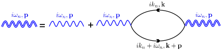
Figure 2: Feynman diagram of the renormalized phonon propagator. The double wavy line and single wavy line represent the renormalized and bare phonon propagator respectively. The solid line represents the bare electron Green’s function.

The Feynman diagram of the phonon self-energy is shown in Fig.2, which can be written as

$$\Pi_{\chi}(i\omega_{n},\mathbf{p})=2\sum_{\eta=\pm}\Pi^{\eta}_{\chi}(i\omega_{n},\mathbf{p})$$ (36)

where the factor 2 accounts for spin degeneracy, and $\Pi^{\eta}_{\chi}(i\omega_{n},\mathbf{p})$ represents the contributions to the phonon self-energy from the valley $\eta$,

$$\Pi^{\eta}_{\chi}(i\omega_{n},\mathbf{p})= \frac{1}{\beta}\sum_{ik_{n},\mathbf{k}}\text{Tr}\Big{[}G^{0}_{\eta,\mathbf{K}_{M1}}(ik_{n},\mathbf{k})\hat{g}^{\dagger}_{\eta,\chi}(\mathbf{p})G^{0}_{\eta,\mathbf{K}_{M2}}(ik_{n}+i\omega_{n},\mathbf{k}+\mathbf{p})\hat{g}_{\eta,\chi}(\mathbf{p})\Big{]},$$ (37)

with $\beta=1/k_{B}T$.

The bare electron Green’s function near the Moire Dirac point $\mathbf{K}_{M_{i}}$ of valley $\eta$ is

$$G_{\eta,\mathbf{K}_{Mi}}^{0}(ik_{n},\mathbf{k})=\frac{(ik_{n}+\mu)\sigma_{0}+v(\mathbf{k}-\mathbf{K}_{Mi})\cdot\bm{\sigma}_{\eta}}{(ik_{n}+\mu)^{2}-E_{\mathbf{k}-\mathbf{K}_{Mi}}^{2}},$$ (38)

where $\bm{\sigma}_{\eta}\equiv(\eta\sigma_{x},-\sigma_{y})$, $E_{\mathbf{k}-\mathbf{K}_{Mi}}\equiv v\absolutevalue{\mathbf{k}-\mathbf{K}_{Mi}}$ represents the upper band spectrum of Eq.(12), $ik_{n}$ denotes the electronic Matsubara frequency and $\mu$ the chemical potential.

For the phonon momentum $\mathbf{p}\approx-\mathbf{q}_{1}$, the phonon self-energy after the sum over the electron Matsubara frequency $ik_{n}$ becomes

$$\Pi_{\chi}(i\omega_{n},\mathbf{p})=2\sum_{\mathbf{k}}\sum_{t,t^{\prime}=\pm}\sum_{\eta=\pm}\frac{n_{F}(t^{\prime}E_{\mathbf{k}-\mathbf{K}_{\text{M1}}}-\mu)-n_{F}(tE_{\mathbf{k}+\mathbf{p}-\mathbf{K}_{\text{M2}}}-\mu)}{i\omega_{n}+t^{\prime}E_{\mathbf{k}-\mathbf{K}_{M1}}-tE_{\mathbf{k}+\mathbf{p}-\mathbf{K}_{\text{M2}}}}\left|\bra{\mathbf{k}+\mathbf{p},t;\eta}\hat{g}_{\eta,\chi}(\mathbf{p})\ket{\mathbf{k},t^{\prime};\eta}\right|^{2}.$$ (39)

Here, $t,t^{\prime}=\pm 1$ represents the two bands of the effective Hamiltonian Eq.(12), $n_{F}$ is the Fermi distribution function, $\bra{\mathbf{k}+\mathbf{p},t;\eta}\hat{g}_{\eta,\chi}(\mathbf{p})\ket{\mathbf{k},t^{\prime};\eta}$ is the e-phonon scattering matrix from the electronic state $\mathbf{k}$ of band $t^{\prime}$ to the state $\mathbf{k}+\mathbf{p}$ of band $t$ in valley $\eta$ caused by the phonon with polarization $\chi$, as shown in Fig.1b. For $\chi=L,T$, the e-phonon scattering matrices are respectively

$$\left|\bra{\mathbf{k}+\mathbf{p},t;\eta}\hat{g}_{\eta,\chi=L}(\mathbf{p})\ket{\mathbf{k},t^{\prime};\eta}\right|^{2} = \frac{\absolutevalue{g_{L,\mathbf{p}}}^{2}}{2}\left[\alpha_{1}^{2}-tt^{\prime}\alpha_{1}^{2}\cos{(\varphi_{\mathbf{k}+\mathbf{p}}+\varphi_{\mathbf{k}})}\right],$$ (40)

$$\left|\bra{\mathbf{k}+\mathbf{p},t;\eta}\hat{g}_{\eta,\chi=T}(\mathbf{p})\ket{\mathbf{k},t^{\prime};\eta}\right|^{2} = \frac{\absolutevalue{g_{T,\mathbf{p}}}^{2}}{2}[(\alpha_{0}^{2}+\alpha_{1}^{2})+tt^{\prime}\alpha_{0}^{2}\cos{(\varphi_{\mathbf{k}+\mathbf{p}}-\varphi_{\mathbf{k}})}$$ (41)

$$+tt^{\prime}\alpha_{1}^{2}\cos{(\varphi_{\mathbf{k}+\mathbf{p}}+\varphi_{\mathbf{k}})}+2t^{\prime}\eta\alpha_{0}\alpha_{1}\cos{\varphi_{\mathbf{k}}}+2t\eta\alpha_{0}\alpha_{1}\cos{\varphi_{\mathbf{k}+\mathbf{p}}}],$$

where $\varphi_{\mathbf{k}}$ and $\varphi_{\mathbf{k}+\mathbf{p}}$ are the polar angles of the vectors $\mathbf{k}-\mathbf{K}_{\text{M1}}$ and $\mathbf{k}+\mathbf{p}-\mathbf{K}_{\text{M2}}$ respectively.

We separate the phonon self-energy in Eq.(LABEL:eq:Phonon_self_energy) to two parts in the calculation: One part corresponds to the contribution at zero temperature and zero doping, which we denote as the vacuum part $\Pi^{\rm vac}_{\chi}$; the other part corresponds to the contribution at finite temperature and finite doping, which is denoted as the matter part $\Pi^{\rm mat}_{\chi}$. We then get after the analytic continuation $i\omega_{n}\to\omega+i0^{+}$,

$$\Pi^{\text{vac}}_{\chi=T}(\omega,\mathbf{p}) = \frac{4\absolutevalue{g_{T,\mathbf{p}}}^{2}}{(2\pi)^{2}}\int d\mathbf{k}\left(\frac{1}{\omega-E_{\mathbf{k}-\mathbf{K}_{\text{M1}}}-E_{\mathbf{k}+\mathbf{p}-\mathbf{K}_{\text{M2}}}+i0^{+}}-\frac{1}{\omega+E_{\mathbf{k}-\mathbf{K}_{\text{M1}}}+E_{\mathbf{k}+\mathbf{p}-\mathbf{K}_{\text{M2}}}+i0^{+}}\right)$$ (42)

$$\times\frac{1}{2}\left[(\alpha_{0}^{2}+\alpha_{1}^{2})-\alpha_{0}^{2}\cos{(\varphi_{\mathbf{k}+\mathbf{p}}-\varphi_{\mathbf{k}})}-\alpha_{1}^{2}\cos{(\varphi_{\mathbf{k}+\mathbf{p}}+\varphi_{\mathbf{k}})}\right],$$

$$\Pi^{\text{vac}}_{\chi=L}(\omega,\mathbf{p}) = \frac{4\absolutevalue{g_{L,\mathbf{p}}}^{2}}{(2\pi)^{2}}\int d\mathbf{k}\left(\frac{1}{\omega-E_{\mathbf{k}-\mathbf{K}_{\text{M1}}}-E_{\mathbf{k}+\mathbf{p}-\mathbf{K}_{\text{M2}}}+i0^{+}}-\frac{1}{\omega+E_{\mathbf{k}-\mathbf{K}_{\text{M1}}}+E_{\mathbf{k}+\mathbf{p}-\mathbf{K}_{\text{M2}}}+i0^{+}}\right)$$ (43)

$$\times\frac{1}{2}\left[\alpha_{1}^{2}+\alpha_{1}^{2}\cos{(\varphi_{\mathbf{k}+\mathbf{p}}+\varphi_{\mathbf{k}})}\right],$$

$$\Pi^{\text{mat}}_{\chi}(\omega,\mathbf{p}) = \Pi_{\chi}(\omega,\mathbf{p})-\Pi^{\text{vac}}_{\chi}(\omega,\mathbf{p}).$$ (44)

In the case $v\gg s$ and the temperature much less than the bandwidth, the deviation of the total phonon self-energy $\Pi_{\chi}$ from the vacuum part $\Pi^{\text{vac}}_{\chi=T}$ is very small and we can get the information of the Kohn anomaly analytically from $\Pi^{\text{vac}}_{\chi=T}$. At zero doping, only inter-band scattering processes can happen, i.e., $tt^{\prime}=-1$ in Eq.(LABEL:eq:Phonon_self_energy). The vacuum part of the phonon self-energy can be obtained as

$$\text{Re}\left[\Pi^{\text{vac}}_{\chi=T}(\omega,\mathbf{p})\right]=\absolutevalue{g_{T,\mathbf{p}}}^{2}\frac{\absolutevalue{\mathbf{p}+\mathbf{q}_{1}}}{2\pi v}\Bigg{\{}-\frac{\alpha_{1}^{2}}{4}(\Lambda-1)-\frac{\alpha_{1}^{2}}{4}(-\frac{1}{\Lambda}+1)$$

$$\ -\frac{\left(\alpha_{0}^{2}+\alpha_{1}^{2}(\omega^{2}/v^{2}|\mathbf{p}+\mathbf{q}_{1}|^{2}\right)}{\sqrt{1-\omega^{2}/v^{2}|\mathbf{p}+\mathbf{q}_{1}|^{2}}}\sum_{t=\pm}\left[\arctan(\frac{\Lambda+t\omega/v|\mathbf{p}+\mathbf{q}_{1}|}{\sqrt{1-\omega^{2}/v^{2}|\mathbf{p}+\mathbf{q}_{1}|^{2}}})-\arctan(\frac{1+t\omega/v|\mathbf{p}+\mathbf{q}_{1}|}{\sqrt{1-(\omega)^{2}/v^{2}|\mathbf{p}+\mathbf{q}_{1}|^{2}}})\right]\Bigg{\}},$$ (45)

$$\text{Re}\left[\Pi^{\text{vac}}_{\chi=L}(\omega,\mathbf{p})\right]=\absolutevalue{g_{L,\mathbf{p}}}^{2}\frac{\absolutevalue{\mathbf{p}+\mathbf{q}_{1}}}{2\pi v}\Bigg{\{}-\frac{\alpha_{1}^{2}}{2}\Lambda+\frac{\alpha_{1}^{2}}{2}\frac{1}{\Lambda}$$

$$+\alpha_{1}^{2}\frac{\left(1+\omega^{2}/v^{2}|\mathbf{p}+\mathbf{q}_{1}|^{2}\right)}{\sqrt{1-\omega^{2}/v^{2}|\mathbf{p}+\mathbf{q}_{1}|^{2}}}\sum_{t=\pm}\left[\arctan(\frac{\Lambda+t\omega/v|\mathbf{p}+\mathbf{q}_{1}|}{\sqrt{1-\omega^{2}/v^{2}|\mathbf{p}+\mathbf{q}_{1}|^{2}}})-\arctan(\frac{1+t\omega/v|\mathbf{p}+\mathbf{q}_{1}|}{\sqrt{1-(\omega)^{2}/v^{2}|\mathbf{p}+\mathbf{q}_{1}|^{2}}})\right]\Bigg{\}}$$ (46)

and

$$\text{Im}\left[\Pi^{\text{vac}}_{\chi=T}(\omega,\mathbf{p})\right] = \absolutevalue{g_{T,\mathbf{p}}}^{2}\frac{\absolutevalue{\mathbf{p}+\mathbf{q}_{1}}}{4v}\frac{\left(\alpha_{0}^{2}+\alpha_{1}^{2}(\omega)^{2}/E_{\mathbf{p}+\mathbf{q}_{1}}^{2}\right)}{\sqrt{\absolutevalue{(\omega)^{2}/E_{\mathbf{p}+\mathbf{q}_{1}}^{2}-1}}}\left[-\Theta(\omega-E_{\mathbf{p}+\mathbf{q}_{1}})+\Theta(-\omega-E_{\mathbf{p}+\mathbf{q}_{1}})\right],$$ (47)

$$\text{Im}\,\left[\Pi^{\text{vac}}_{\chi=L}(\omega,\mathbf{p})\right] = \absolutevalue{g_{L,\mathbf{p}}}^{2}\alpha_{1}^{2}\frac{\absolutevalue{\mathbf{p}+\mathbf{q}_{1}}}{4v}\sqrt{\absolutevalue{\frac{\omega^{2}}{v^{2}\absolutevalue{\mathbf{p}+\mathbf{q}_{1}}^{2}}-1}}\left[-\Theta(\omega-v\absolutevalue{\mathbf{p}+\mathbf{q}_{1}})+\Theta(-\omega-v\absolutevalue{\mathbf{p}+\mathbf{q}_{1}})\right]$$ (48)

where $\Lambda=1+\frac{2E_{c}}{v\absolutevalue{\mathbf{p}+\mathbf{q}_{1}}}+\sqrt{\Big{(}1+\frac{2E_{c}}{v\absolutevalue{\mathbf{p}+\mathbf{q}_{1}}}\Big{)}^{2}+1}$ with $E_{c}\sim vq_{1}$ the high energy cutoff of the Moire electrons, and $\Theta(\omega-E_{\mathbf{p}+\mathbf{q}_{1}})$ is the Heaviside step function.

The matter part of the phonon self-energy comes from the contribution of finite temperature and finite doping. For the $\rm TA$ mode, it is

$$\Pi^{\text{mat}}_{\chi=T}(i\omega_{n},\mathbf{p}) = \frac{4\absolutevalue{g_{T,\mathbf{p}}}^{2}}{(2\pi)^{2}}\int d\mathbf{k}\sum_{t,t^{\prime}=\pm 1}\frac{n_{F}(t^{\prime}E_{\mathbf{k}-\mathbf{K}_{\text{M1}}}-\mu)-n_{F}(tE_{\mathbf{k}+\mathbf{p}-\mathbf{K}_{\text{M2}}}-\mu)-\delta_{t,-t^{\prime}}(\delta_{t^{\prime},-1}-\delta_{t,-1})}{i\omega_{n}+t^{\prime}E_{\mathbf{k}-\mathbf{K}_{\text{M1}}}-tE_{\mathbf{k}+\mathbf{p}-\mathbf{K}_{\text{M2}}}}$$ (49)

$$\frac{1}{2}\left[(\alpha_{0}^{2}+\alpha_{1}^{2})+tt^{\prime}\alpha_{0}^{2}\cos{(\varphi_{\mathbf{k}+\mathbf{p}}-\varphi_{\mathbf{k}})}+tt^{\prime}\alpha_{1}^{2}\cos{(\varphi_{\mathbf{k}+\mathbf{p}}+\varphi_{\mathbf{k}})}\right].$$

Since $1-n_{F}(-E_{\mathbf{k}-\mathbf{K}_{\text{M1}}}-\mu)=n_{F}(E_{\mathbf{k}-\mathbf{K}_{\text{M1}}}+\mu)$, the above equation can be simplified as

$$\Pi^{\text{mat}}_{\chi=T}(i\omega_{n},\mathbf{p})=\frac{4\absolutevalue{g_{T,\mathbf{p}}}^{2}}{(2\pi)^{2}}\int_{0}^{\infty}\frac{d(E_{\mathbf{k}-\mathbf{K}_{\text{M1}}})}{v^{2}}\Big{(}n_{F}(E_{\mathbf{k}-\mathbf{K}_{\text{M1}}}+\mu)+n_{F}(E_{\mathbf{k}-\mathbf{K}_{\text{M1}}}-\mu)\Big{)}\left[\sum_{t=\pm}\int_{0}^{2\pi}d\varphi_{\mathbf{k}}\,F_{t,\chi=T}(\mathbf{k},\mathbf{p},i\omega_{n})\right]$$ (50)

where

$$F_{t,\chi=T}(i\omega_{n},\mathbf{k},\mathbf{p}) = \frac{1}{\big{(}E_{\mathbf{k}-\mathbf{K}_{\text{M1}}}+t(i\omega_{n})\big{)}^{2}-E_{\mathbf{k}+\mathbf{p}-\mathbf{K}_{\text{M2}}}^{2}}\Big{[}(\alpha_{0}^{2}+\alpha_{1}^{2})\big{(}E_{\mathbf{k}-\mathbf{K}_{\text{M1}}}+t(i\omega_{n})\big{)}E_{\mathbf{k}-\mathbf{K}_{\text{M1}}}$$ (51)

$$+ \alpha_{0}^{2}E_{\mathbf{k}-\mathbf{K}_{\text{M1}}}E_{\mathbf{k}+\mathbf{p}-\mathbf{K}_{\text{M2}}}\cos{(\varphi_{\mathbf{k}+\mathbf{p}}-\varphi_{\mathbf{k}})}+\alpha_{1}^{2}E_{\mathbf{k}-\mathbf{K}_{\text{M1}}}E_{\mathbf{k}+\mathbf{p}-\mathbf{K}_{\text{M2}}}\cos{(\varphi_{\mathbf{k}+\mathbf{p}}+\varphi_{\mathbf{k}})}\Big{]},$$

and the integration over the angel $\varphi_{\mathbf{k}}$ can be worked out as

$$\Phi_{T}(i\omega_{n},\mathbf{p},E_{\mathbf{k}-\mathbf{k}_{M1}})\equiv\sum_{t=\pm}\int_{0}^{2\pi}d\varphi_{\mathbf{k}}\,F_{t,\chi=T}(\mathbf{k},\mathbf{p},i\omega_{n})=2\pi\Big{[}\alpha_{1}^{2}\frac{(i\omega_{n})^{2}}{v^{2}|\mathbf{p}+\mathbf{q}_{1}|^{2}}+\alpha_{0}^{2}\Big{]}\sum_{t=\pm}\bigg{\{}-\frac{1}{2}$$

$$+\frac{2E_{\mathbf{k}-\mathbf{K}_{\text{M1}}}^{2}+2t(i\omega_{n})\,E_{\mathbf{k}-\mathbf{K}_{\text{M1}}}+\frac{1}{2}\left((i\omega_{n})^{2}-v^{2}|\mathbf{p}+\mathbf{q}_{1}|^{2}\right)}{\sqrt{4\left((i\omega_{n})^{2}-v^{2}|\mathbf{p}+\mathbf{q}_{1}|^{2}\right)E_{\mathbf{k}-\mathbf{K}_{\text{M1}}}^{2}+4t(i\omega_{n})\left((i\omega_{n})^{2}-v^{2}|\mathbf{p}+\mathbf{q}_{1}|^{2}\right)E_{\mathbf{k}-\mathbf{K}_{\text{M1}}}+\left((i\omega_{n})^{2}-v^{2}|\mathbf{p}+\mathbf{q}_{1}|^{2}\right)^{2}}}\bigg{\}}.$$ (52)

Similarly, for the $\rm LA$ mode, the matter part of the phonon self-energy is

$$\Pi^{\text{mat}}_{\chi=L}(i\omega_{n},\mathbf{p}) = \frac{4\absolutevalue{g_{T,\mathbf{p}}}^{2}}{(2\pi)^{2}}\int d\mathbf{k}\sum_{t,t^{\prime}=\pm 1}\frac{n_{F}(t^{\prime}E_{\mathbf{k}-\mathbf{K}_{\text{M1}}}-\mu)-n_{F}(tE_{\mathbf{k}+\mathbf{p}-\mathbf{K}_{\text{M2}}}-\mu)-\delta_{t,-t^{\prime}}(\delta_{t^{\prime},-1}-\delta_{t,-1})}{i\omega_{n}+t^{\prime}E_{\mathbf{k}-\mathbf{K}_{\text{M1}}}-tE_{\mathbf{k}+\mathbf{p}-\mathbf{K}_{\text{M2}}}}$$

$$\quad\quad\quad\quad\quad\quad\frac{1}{2}\left[\alpha_{1}^{2}-tt^{\prime}\alpha_{1}^{2}\cos{(\varphi_{\mathbf{k}+\mathbf{p}}+\varphi_{\mathbf{k}})}\right]$$

$$= \frac{4\absolutevalue{g_{T,\mathbf{p}}}^{2}}{(2\pi)^{2}}\int_{0}^{\infty}\frac{d(E_{\mathbf{k}-\mathbf{K}_{\text{M1}}})}{v^{2}}\Big{(}n_{F}(E_{\mathbf{k}-\mathbf{K}_{\text{M1}}}+\mu)+n_{F}(E_{\mathbf{k}-\mathbf{K}_{\text{M1}}}-\mu)\Big{)}\left[\sum_{t=\pm}\int_{0}^{2\pi}d\varphi_{\mathbf{k}}\,F_{t,\chi=L}(i\omega_{n},\mathbf{k},\mathbf{p})\right]$$

where

$$F_{t,\chi=L}(i\omega_{n},\mathbf{k},\mathbf{p})=$$

$$\quad\quad\frac{\alpha_{1}^{2}}{\big{(}E_{\mathbf{k}-\mathbf{K}_{\text{M1}}}+t(i\omega_{n})\big{)}^{2}-E_{\mathbf{k}+\mathbf{p}-\mathbf{K}_{\text{M2}}}^{2}}\Big{[}\big{(}E_{\mathbf{k}-\mathbf{K}_{\text{M1}}}+t(i\omega_{n})\big{)}E_{\mathbf{k}-\mathbf{K}_{\text{M1}}}-E_{\mathbf{k}-\mathbf{K}_{\text{M1}}}E_{\mathbf{k}+\mathbf{p}-\mathbf{K}_{\text{M2}}}\cos{(\varphi_{\mathbf{k}+\mathbf{p}}+\varphi_{\mathbf{k}})}\Big{]}$$ (54)

and

$$\Phi_{L}(i\omega_{n},\mathbf{p},E_{\mathbf{k}-\mathbf{k}_{M1}})\equiv\sum_{t=\pm 1}\int_{0}^{2\pi}d\varphi_{\mathbf{k}}\,F_{t,\chi=L}(i\omega_{n},\mathbf{k},\mathbf{p})=2\pi\alpha_{1}^{2}\frac{(i\omega_{n})^{2}}{v^{2}|\mathbf{p}+\mathbf{q}_{1}|^{2}}\sum_{t=\pm 1}$$ (55)

$$\left[\frac{1}{2}+\frac{\left(v^{2}|\mathbf{p}+\mathbf{q}_{1}|^{2}/(i\omega_{n})^{2}-1\right)\left(2E_{\mathbf{k}-\mathbf{K}_{\text{M1}}}^{2}+2t(i\omega_{n})\,E_{\mathbf{k}-\mathbf{K}_{\text{M1}}}+\frac{1}{2}(i\omega_{n})^{2}\right)}{\sqrt{4\left((i\omega_{n})^{2}-v^{2}|\mathbf{p}+\mathbf{q}_{1}|^{2}\right)E_{\mathbf{k}-\mathbf{K}_{\text{M1}}}^{2}+4t(i\omega_{n})\left((i\omega_{n})^{2}-v^{2}|\mathbf{p}+\mathbf{q}_{1}|^{2}\right)E_{\mathbf{k}-\mathbf{K}_{\text{M1}}}+\left((i\omega_{n})^{2}-v^{2}|\mathbf{p}+\mathbf{q}_{1}|^{2}\right)^{2}}}\right].$$

At finite temperature, it is hard to get an analytic result of the integration in Eq.(50) and (IV.1). We then evaluate $\Pi^{\rm mat}_{\chi}$ numerically and add it to the total phonon self-energy $\Pi_{\chi}$.

IV.2 Dynamic Kohn anomaly for the TA mode

We first consider the case with zero doping. The renormalized phonon frequency due to the e-phonon interaction can be obtained from the pole of the renormalized phonon GF, $D_{\chi}(i\omega_{n},\mathbf{p})=D^{0}_{\chi}(i\omega_{n},\mathbf{p})/[1-D^{0}_{\chi}(i\omega_{n},\mathbf{p})\Pi_{\chi}(i\omega_{n},\mathbf{p})]$, where $D^{0}_{\chi}(i\omega_{n},\mathbf{p})=2\omega_{0,\mathbf{p},\chi}/[(i\omega_{n})^{2}-\omega^{2}_{0,\mathbf{p},\chi}]$ is the bare phonon propagator. The renormalized phonon frequency $\omega_{\mathbf{p},\chi}$ then satisfies

$$\omega_{\mathbf{p},\chi}^{2}/\omega^{2}_{0,\mathbf{p},\chi}-1=2\rm Re[\Pi_{\chi}(\omega,\mathbf{p})]/\omega_{0,\mathbf{p},\chi},$$ (56)

where the phonon self-energy $\Pi_{\chi}(\omega,\mathbf{p})$ is worked out in the last subsection.

Figure.3(a)-(e) and Fig.5(a)-(e) show the real part of $\Pi^{\rm vac}_{\chi}$ for the TA and LA mode respectively. From Eq.(45) and (46), the real part of $\Pi^{\rm vac}_{\chi}$ for both the TA and LA phonon diverges at

$$\omega=v|\mathbf{p}+\mathbf{q}_{1}|.$$ (57)

In this condition, the imaginary part of the self-energy for the TA mode in Eq.(47) diverges too, whereas the imaginary of the self-energy for the LA mode is finite. For the twist angle away from the magic angle, the electron velocity $v$ is much greater than the phonon velocity $s$ and the phonon frequency $\omega$ is negligible in Eq.(57). The Kohn anomaly, i.e., the divergence of the self-energy then occurs at $\mathbf{p}\approx-\mathbf{q}_{1}$ due to the nesting of the Fermi points at zero doping.

For twist angle close to the magic angle, the two bands of the Hamiltonan Eq.(12) becomes very narrow. In this case, the phonon energy $\omega_{0}=sp$ is not negligible compared to the electron energy and the dynamics of the phonon becomes important. For the perturbative self-energy $\Pi_{\chi}(\omega,\mathbf{p})$, we can set $\omega=\omega_{0}$. The divergence of the self-energy then occurs at phonon momentum $\mathbf{p}$ that satisfies

$$sp=v|\mathbf{p}+\mathbf{q}_{1}|.$$ (58)

The momentum mismatch of the nesting condition $\delta\mathbf{q}\equiv\mathbf{p}+\mathbf{q}_{1}$ is compensated by the dynamics of the phonon.

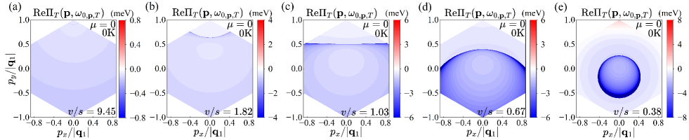
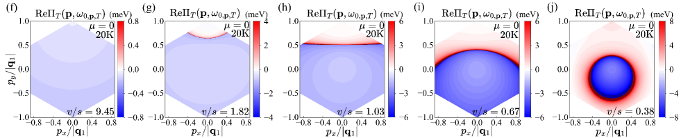
Figure 3: The real part of the TA phonon self-energy at zero doping: (a)-(e) at zero temperature and (f)-(j) at $T=20K$ for different $v/s$.

The orbit of the phonon momentum $\mathbf{p}$ satisfying Eq.(57) is a circle in momentum space with the center $(p_{x},p_{y})=(0,\frac{v^{2}}{v^{2}-s^{2}}q_{1})$ and radius $\frac{sv}{|s^{2}-v^{2}|}q_{1}$ for $s\neq v$ and a straight line for $s=v$. This is clearly seen from the divergence lines in Fig.3(a)-(e) for the vacuum part of the TA self-energy with different $v/s$. Figure 4(a) shows the cut of the TA phonon self-energy along the line $p_{x}=0$ from Fig.3(a)-(e). It is clear that with the decrease of $v/s$, the phonon momentum where the divergence of the self-energy occurs moves from $p_{y}=q_{1}$ towards $p_{y}=0$.

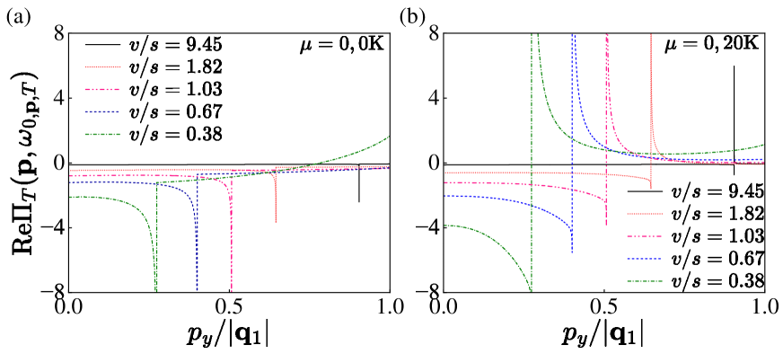
Figure 4: The real part of the TA phonon self-energy at (a)$T=0K$ and (b)$T=20K$ along the line $p_{x}=0$ for different $v/s$.

We should note that since we have set the e-phonon coupling constant $g_{\chi}(\mathbf{p})\approx g_{\chi}(-\mathbf{q}_{1})$ in the calculation, the result of the self-energy in Eq.(45) and (46) is quantitatively accurate only near $\mathbf{p}\approx-\mathbf{q}_{1}$. However, the divergence condition in Eq.(57) comes from the energy conservation and should still be valid for $\mathbf{p}$ deviates from $-\mathbf{q}_{1}$. A particularly interesting question is whether the dynamic Kohn anomaly happens when the electron bands are flat. Here we can see that for the flat bands, i.e., $v/s=0$, the dynamic Kohn anomaly could only happen at phonon momentum $\mathbf{p}=0$ because in this case the e-phonon scattering is elastic. However, for the acoustic mode, either TA or LA mode, the bare phonon frequency at $\mathbf{p}=0$ is already zero. So the phonon softening can no longer happen, i.e., the dynamic Kohn anomaly of the acoustic modes does not occur for the completely flat electron bands.

We next study the effect of the matter part due to the finite temperature. For $T$ much less than the electron bandwidth $\Lambda\sim vq_{1}$, the correction to the phonon self-energy by the finite temperature is very small, i.e., we can neglect the matter part of the phonon self-energy and only include the vacuum part. However, for TBG, the electron bandwidth can become very small by tuning the twist angle. When the bandwidth is comparable to the temperature, the contribution from the matter part becomes significant and one needs to include this part in the phonon self energy. It is hard to get an analytic result for the matter part of the self-energy. For the reason, we compute the matter part of the TA phonon self-energy numerically and show the TA phonon self-energy including the matter part at $T=20K$ in Fig.3(f)-(j) for different $v/s$. The cut of the phonon self-energy at $T=20K$ along the line $p_{x}=0$ is shown in Fig.4(b). It turns out that the matter part of the TA phonon mode has opposite sign as the vacuum part. From Fig.3 and Fig.4, we can see that the finite temperature does not change the position of the phonon momentum where the Kohn anomaly occurs. However, it may change the value of the phonon self-energy significantly. Particularly, when the temperature is comparable to the electron bandwidth, the phonon self-energy may change sign at the momenta where the dynamic Kohn anomaly occurs, which results in a change from phonon softening to phonon hardening for momenta on the two sides of the Kohn anomaly, as shown in Fig.3 and Fig.4.

IV.3 Dynamic Kohn anomaly for the LA mode

The self-energy of the LA phonon mode at zero temperature is shown in Fig.5 for different $v/s$. Different from the TA mode, the peak of the LA phonon self-energy near the Kohn anomaly can be positive for the LA mode even at zero temperature, as can be also seen from the cut of self-energy along the line $p_{x}=0$ in Fig.6a. On the other hand, the matter part of the LA phonon self-energy is small and positive. It vanishes at the Kohn anomaly instead of diverging. For the reason, the finite temperature does not change the LA phonon self-energy qualitatively, as shown in Fig.5 and Fig.6.

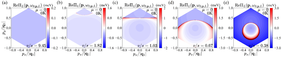
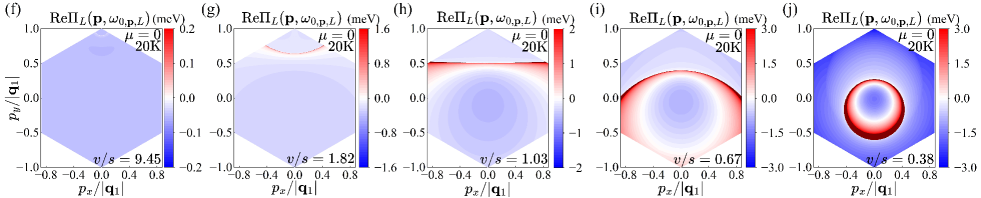
Figure 5: The real part of the LA phonon self-energy: (a)-(e) at zero temperature and (f)-(j) at $T=20K$ for different $v/s$.

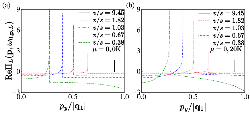
Figure 6: The real part of the phonon self-energy for the LA mode along the line $p_{x}=0$ in the BZ (a) at $T=0$ and (b) at $T=20K$.

IV.4 Dynamic Kohn anomaly at finite doping

The above results are obtained at zero doping, i.e., the electron Fermi energy crosses the Moire Dirac points. In this subsection, we discuss the dynamic Kohn anomaly at finite doping. For simplicity, we only show the phonon self-energy of the TA mode at finite doping and zero temperature. For the same doping at two Moire Dirac points, the TA phonon self-energy can be obtained by setting $\mu$ finite in Eq.(50). In this case the divergence condition of the TA phonon self-energy is the same as for the zero doping. We show the plot of the TA phonon self-energy at finite doping in Fig.7. We can see that the finite doping may change the sign of the TA phonon self-energy near the Kohn anomaly. This effect is similar to that of finite temperature because both doping and finite temperature may activate the electrons at energy $E>0$ and result in a positive matter part of the TA phonon self-energy near the Kohn anomaly.

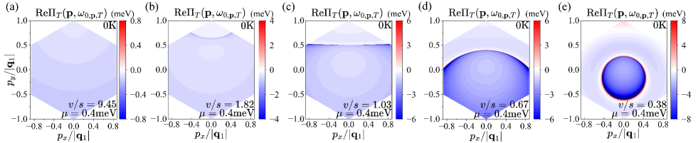
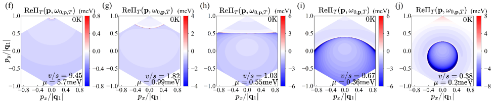
Figure 7: (a)-(e) The self-energy of the TA mode at zero temperature and same finite chemical potential $\mu=0.4\rm meV$ for different $v/s$. (f)-(j)The self-energy of the TA mode at zero temperature and same filling factor $\nu=0.75$ for different $v/s$.

V Discussions and conclusion

The dynamic Kohn anomaly in TBG is different from the Kohn anomaly observed in ordinary metal, for which a cusp in the phonon dispersion appears at $q=2k_{F}$. The difference originates from the relativistic chiral band structure of the TBG we employed in the continuum model. Similar band structure also applies for graphene and results in a novel dynamic Kohn anomaly in such system, as studied in Ref.[48]. For both the graphene and undoped TBG, the dynamics of the phonon can not be neglected. This is revealed in the dependence on the phonon frequency of the phonon wave vector for which the Kohn anomaly occurs. However, the dynamic Kohn anomaly in graphene in Ref.[48] is also different from that in TBG we obtained in this work. The former comes from the intravalley e-phonon scatterings in graphene, whereas the latter comes from the inter-valley electron scatterings mediated by phonons in TBG. For the reason, the phonon wave-vectors where the dynamic Kohn anomaly occurs are different in the two systems. For graphene, the Kohn anomaly occurs at $q=\omega/v$ or $2k_{F}-\omega/q$ for the TO and LO phonons.

Another system which has similar dynamic Kohn anomaly as TBG is the WSM. The Kohn anomaly due to inter-Weyl-node electron scatterings by phonons in tantalum phosphide (TaP) has been studied both theoretically and experimentally in Ref.[49] The phonon momenta where the dynamic Kohn anomaly occurs in TaP satisfy the same condition as for TBG, i.e., Eq.(57). However, since the TaP WSM is three dimensional, the power of the divergence at the Kohn anomaly is different in the two systems. Without screening, the phonon self-energy in TaP diverges logarithmically at the Kohn anomaly, whereas in TBG, the self energy diverges as a power law as shown in Eq.(45) and (46). Besides, in WSM, the electron velocity is usually much greater than the phonon velocity. For the reason, the phonon wave-vector for which the Kohn anomaly occurs is very close to the nesting momentum, i.e., the distance of the two Weyl nodes. However, in TBG, by tuning the twisting angle, the electron velocity may become smaller than the phonon velocity. In this case, the phonon momenta for which the dynamic Kohn anomaly occurs deviate significantly from the nesting momentum or the distance of the two Moire Dirac points. At magic angle when the two electron bands crossing the Fermi energy become almost flat, the dynamic Kohn anomaly disappears because the inter-valley e-phonon scattering cannot satisfy the energy and momentum conservation at the same time.

The Kohn anomaly can be observed through inelastic x-ray and neutron scattering, as done on WSM TaP. The softening or hardening of the phonon frequency may result in modification of the superconductivity or other phonon-related properties in the TBG, which we will leave for a future study.

In conclusion, we studied the e-phonon interaction of the acoustic phonon modes with the electrons in an effective two band system in the TBG under the continuum model. Based on this model, we studied the effect of the e-phonon interaction on the phonon frequency, i.e., the dynamic Kohn anomaly. We show that the Kohn anomaly in the TBG has different properties from that in ordinary metal and other relativistic materials, such as graphene and WSM. Moreover, by tuning the twist angle, the dynamic Kohn anomaly in TBG is also tunable. Especially, at magic angle when the two bands crossing the Fermi energy becomes almost flat, the dynamic Kohn anomaly in TBG disappears. The Kohn anomaly in TBG may be detected by inelastic x-ray or neutron scatterings.

VI Acknowledgement

This work is supported by the National NSF of China under Grant No. 11974166 and the NSF of Jiangsu Province under Grant No.BK20231398.

References

• [1] Cao Y, Fatemi V, Fang S, Watanabe K, Taniguchi T, Kaxiras E and Jarillo-Herrero P 2018 Nature 556 43–50
• [2] Po H C, Zou L, Vishwanath A and Senthil T 2018 Phys. Rev. X 8, 031089
• [3] Lu X, Stepanov P, Yang W, Xie M, Aamir M A, Das I, Urgell C, Watanabe K, Taniguchi T, Zhang G, Bachtold A, MacDonald A H and Efetov D K 2019 Nature 574 653–7
• [4] Yankowitz M, Chen S, Polshyn H, Zhang Y, Watanabe K, Taniguchi T, Graf D, Young A F and Dean C R 2019 Science 363 1059–64
• [5] Stepanov P, Das I, Lu X, Fahimniya A, Watanabe K, Taniguchi T, Koppens F H L, Lischner J, Levitov L and Efetov D K 2020 Nature 583 375–8
• [6] Saito Y, Ge J, Watanabe K, Taniguchi T and Young A F 2020 Nat. Phys. 16 926–30
• [7] Nuckolls K P, Lee R L, Oh M, Wong D, Soejima T, Hong J P, Călugăru D, Herzog-Arbeitman J, Bernevig B A, Watanabe K, Taniguchi T, Regnault N, Zaletel M P and Yazdani A 2023 Nature 620 525–32
• [8] Ledwith P J, Tarnopolsky G, Khalaf E and Vishwanath A 2020 Phys. Rev. Res. 2 023237
• [9] Repellin C and Senthil T 2020 Phys. Rev. Res. 2 023238
• [10] Wilhelm P, Lang T C and Läuchli A M 2021 Phys. Rev. B 103 125406
• [11] Xie Y, Pierce A T, Park J M, Parker D E, Khalaf E, Ledwith P, Cao Y, Lee S H, Chen S, Forrester P R, Watanabe K, Taniguchi T, Vishwanath A, Jarillo-Herrero P and Yacoby A 2021 Nature 600 439–43
• [12] Stepanov P, Xie M, Taniguchi T, Watanabe K, Lu X, MacDonald A H, Bernevig B A and Efetov D K 2021 Phys. Rev. Lett. 127 197701
• [13] Parker D, Ledwith P, Khalaf E, Soejima T, Hauschild J, Xie Y, Pierce A, Zaletel M P, Yacoby A and Vishwanath A 2021 arXiv:2112.13837
• [14] Cao Y, Fatemi V, Demir A, Fang S, Tomarken S L, Luo J Y, Sanchez-Yamagishi J D, Watanabe K, Taniguchi T, Kaxiras E, Ashoori R C and Jarillo-Herrero P 2018 Nature 556 80–84
• [15] Sharpe A L, Fox E J, Barnard A W, Finney J, Watanabe K, Taniguchi T, Kastner M A and Goldhaber-Gordon D 2019 Science 365 605–8
• [16] Nuckolls K P, Oh M, Wong D, Lian B, Watanabe K, Taniguchi T, Bernevig B A and Yazdani A 2020 Nature 588 610–5
• [17] Serlin M, Tschirhart C L, Polshyn H, Zhang Y, Zhu J, Watanabe K, Taniguchi T, Balents L and Young A F 2020 Science 367 900–3
• [18] Choi Y, Kim H, Peng Y, Thomson A, Lewandowski C, Polski R, Zhang Y, Arora H S, Watanabe K, Taniguchi T, Alicea J and Nadj-Perge S 2020 arXiv:2008.11746
• [19] Sharpe A L, Fox E J, Barnard A W, Finney J, Watanabe K, Taniguchi T, Kastner M A and Goldhaber-Gordon D 2021 Nano Lett. 21 4299–304
• [20] Wu S, Zhang Z, Watanabe K, Taniguchi T and Andrei E Y 2021 Nat. Mater. 20 488–94
• [21] Park J M, Cao Y, Watanabe K, Taniguchi T and Jarillo-Herrero P 2021 Nature 592 43–8
• [22] Das I, Lu X, Herzog-Arbeitman J, Song Z-D, Watanabe K, Taniguchi T, Bernevig B A and Efetov D K 2021 Nat. Phys. 17 710–4
• [23] Calugaru D, Regnault N, Oh M, Nuckolls K P, Wong D, Lee R L, Yazdani A, Vafek O and Bernevig B A 2022 Phys. Rev. Lett. 129 117602
• [24] Blason A and Fabrizio M 2022 Phys. Rev. B 106 235112
• [25] Kwan Y H, Wagner G, Soejima T, Zaletel M P, Simon S H, Parameswaran S A and Bultinck N 2021 Phys. Rev. X 11 041063
• [26] Kang J and Vafek O 2018 Phys. Rev. X 8 031088
• [27] Kang J and Vafek O 2019 Phys. Rev. Lett. 122 246401
• [28] Zhang Y-H, Mao D and Senthil T 2019 Phys. Rev. Res. 1 033126
• [29] Repellin C, Dong Z, Zhang Y-H and Senthil T 2020 Phys. Rev. Lett. 124 187601
• [30] Liu J and Dai X 2021 Phys. Rev. B 103 035427
• [31] Bernevig B A, Song Z-D, Regnault N and Lian B 2021 Phys. Rev. B 103 205413
• [32] Lian B, Song Z-D, Regnault N, Efetov D K, Yazdani A and Bernevig B A 2021 Phys. Rev. B 103 205414
• [33] Bernevig B A, Lian B, Cowsik A, Xie F, Regnault N and Song Z-D 2021 Phys. Rev. B 103 205415
• [34] Wu F, MacDonald A H and Martin I 2018 Phys. Rev. Lett. 121 257001
• [35] Lian B, Wang Z and Bernevig B A 2019 Phys. Rev. Lett. 122 257002
• [36] Angeli M, Tosatti E and Fabrizio M 2019 Phys. Rev. X 9 041010
• [37] Cea T and Guinea F 2021 Proceedings of the National Academy of Sciences 118 e2107874118
• [38] Chen C, Nuckolls K P, Ding S, Miao W, Wong D, Oh M, Lee R L, He S, Peng C, Pei D, Li Y, Zhang S, Liu J, Liu Z, Jozwiak C, Bostwick A, Rotenberg E, Li C, Han X, Pan D, Dai X, Liu C, Bernevig B A, Wang Y, Yazdani A and Chen Y 2023 arXiv:2303.14903
• [39] Liu C-X, Chen Y, Yazdani A and Bernevig B A 2024 Phys. Rev. B 110 045133
• [40] Shi H, Miao W and Dai X 2024 arXiv:2402.11824
• [41] Wang Y-J, Zhou G-D, Lian B and Song Z-D 2024 arXiv:2407.11116
• [42] Wang Y-J, Zhou G-D, Peng S-Y, Lian B and Song Z-D 2024 arXiv:2402.00869
• [43] Kwan Y H, Wagner G, Bultinck N, Simon S H, Berg E and Parameswaran S A 2024 Phys. Rev. B 110 085160
• [44] Ochoa H 2019 Phys. Rev. B 100 155426
• [45] Ishizuka H, Fahimniya A, Guinea F and Levitov L 2021 Nano Lett. 21 7465–71
• [46] Davis S M, Wu F and Sarma S D 2023 Phys. Rev. B 107 235155
• [47] Kohn W 1959 Phys. Rev. Lett. 2 393–4
• [48] Tse W-K, Hu B Y-K and Sarma S D 2008 Phys. Rev. Lett. 101 066401
• [49] Nguyen T, Han F, Andrejevic N, Pablo-Pedro R, Apte A, Tsurimaki Y, Ding Z, Zhang K, Alatas A, Alp E E, Chi S, Fernandez-Baca J, Matsuda M, Tennant D A, Zhao Y, Xu Z, Lynn J W, Huang S and Li M 2020 Phys. Rev. Lett. 124 236401
• [50] Ando T 2006 J. Phys. Soc. Jpn. 75 124701
• [51] Mafra D L, Malard L M, Doorn S K, Htoon H, Nilsson J, Castro Neto A H and Pimenta M A 2009 Phys. Rev. B 80 241414
• [52] Gadelha A C, Nadas R, Barbosa T C, Watanabe K, Taniguchi T, Campos L C, Raschke M B and Jorio A 2022 2D Mater. 9 045028
• [53] Baron A Q R, Uchiyama H, Tanaka Y, Tsutsui S, Ishikawa D, Lee S, Heid R, Bohnen K-P, Tajima S and Ishikawa T 2004 Phys. Rev. Lett. 92 197004
• [54] Pouget J P, Hennion B, Escribe-Filippini C and Sato M 1991 Phys. Rev. B 43 8421–30
• [55] Lopes dos Santos J M B, Peres N M R and Castro Neto A H 2007 Phys. Rev. Lett. 99 256802
• [56] Bistritzer R and MacDonald A H 2011 Proc. Natl. Acad. Sci. U.S.A. 108 12233–7
• [57] Tarnopolsky G, Kruchkov A J and Vishwanath A 2019 Phys. Rev. Lett. 122 106405
• [58] Bernevig B A, Song Z-D, Regnault N and Lian B 2021 Phys. Rev. B 103 205411
• [59] Song Z-D and Bernevig B A 2022 Phys. Rev. Lett. 129 047601
• [60] Shi H and Dai X 2022 Phys. Rev. B 106 245129
• [61] de Gail R, Goerbig M O, Guinea F, Montambaux G and Castro Neto A H 2011 Phys. Rev. B 84 045436
• [62] He W-Y, Chu Z-D and He L 2013 Phys. Rev. Lett. 111 066803
• [63] Po H C, Zou L, Senthil T and Vishwanath A 2019 Phys. Rev. B 99 195455
• [64] Koshino M and Nam N N T 2020 Phys. Rev. B 101 195425
• [65] Xie B and Liu J 2023 Phys. Rev. B 108 094115
• [66] Mariani E and von Oppen F 2008 Phys. Rev. Lett. 100 076801
• [67] Suzuura H and Ando T 2002 Phys. Rev. B 65 235412
• [68] Pereira V M and Castro Neto A H 2009 Phys. Rev. Lett. 103 046801
• [69] Guinea F, Katsnelson M I and Geim A K 2010 Nature Phys 6 30–3
• [70] Mariani E and Von Oppen F 2010 Phys. Rev. B 82 195403
• [71] Ochoa H, Castro E V, Katsnelson M I and Guinea F 2012 Physica E: Low-dimensional Systems and Nanostructures 44 963–6