An experiment to test the isotropy of the one-way speed of light.
Abstract
An experimental setup capable, in principle, to test the isotropy of the one way propagation of light to 1 part in (or better), is suggested.
pacs:
04.20.JbI Introduction.
The speed of light in a vacuum is one of the most fundamental quantities in modern physics. It is well known, however, and there has been ample debate in the literature, that while the two way speed of light is experimentally well defined, the one way speed of light cannot be measured as long as speed is conceived as the ratio of distance travelled to time taken for this travel [1]. We shall call this concept of speed as “ballistic”. The problem stems mainly from the fact that the “ballistic” measurement requires the presence of synchronized clocks at each end of the path travelled, and this synchronization uses in turn light signals, creating a circular argument that so far has made this type of measurement invalid.
Going back to the measurement of the two way speed of light, in the typical experiment light is sent from some initial point to a distant mirror, where it is reflected so that it returns to the initial point. By measuring the distance to the mirror, and the time taken for the full trip (which requires only one clock, i.e. no synchronization), the speed is defined as,
| (1) |
In principle, in (1) represents only the average speed of light in the two way trip. This definition contains the implicit assumption that the speed of light is independent of the direction of propagation, that is, that the one way speed of light is isotropic, but this is precisely what the “ballistic” method cannot establish.
We remark that the “ballistic” idea of measuring the speed of light has no consideration of the fact that the propagation of light is fundamentally a wave phenomenon. As such, in a vacuum, in the absence of dispersion, the speed of propagation of a monochromatic wave of period , and wavelength is,
| (2) |
Therefore, we may compute if we can measure both , and . This seems to take us back to the ballistic idea, but we shall argue that this is not the case. Assume we have a plane monochromatic wave propagating in a given direction. By placing a (single) clock at some fixed point, anywhere in the path of the plane wave, we can measure . Assume further that after the measurement of the wave goes through some fixed structure, and that this gives rise to a certain diffraction pattern, that can be observed further along the path of the wave. The fundamental point here is that the diffraction pattern is completely determined by the geometry of the structure and the wavelength of the diffracted light, with no measurement of time involved, or distance travelled. Thus, if the geometry of the structure is known, a measurement of the diffraction pattern provides immediately a measure of the wavelength . Therefore, using the wave properties of the propagation of light we can obtain in (2), with no synchronization involved.
In practice, in (1) can be measured to much larger accuracy than what (2) could provide. However, as just discussed, the two values of should coincide if the isotropy assumption is valid. As it turns out, and will be the main subject of this paper, the ideas behind (2) can be better used, not to obtain , but rather to test the isotropy of . As will be discussed in what follows, this does not even require measuring times or distances, as only intensities will be involved. As we shall show, even a simple setup could be used to test this isotropy to the order of 1 part in or , and possibly, even better.
In the next Section we review the basics of the diffraction of light by a diffraction grating. Then, in Section III we present our basic idea, which, as explained there, is based on the interference of two separate monochromatic but coherent diffracted beams, which are setup in such a way that they move in opposite directions as the wavelength of the diffracted light changes. In Section IV we discuss several concrete examples, assigning definite numerical values to the different parameters involved, and show that the setup could, in principle, display a sensitivity to changes in , and therefore, for fixed , to , in the order of one part in . We discuss a sketch of what could be a concrete experimental arrangement in Section V. We close with some final comments in Section VI.
We have also added an Appendix with two Sections, where we consider a slightly more general case regarding the experimental parameters and show, both theoretically and with an explicit example, that the essential results regarding the sensitivity of the proposed setup are not modified in this case.
The final conclusion is that this type of experimental arrangement might provide either an upper bound to a possible anisotropy in the one way propagation, and therefore a measure of the one way speed of light to that accuracy, or, on the contrary, establish the existence of an anisotropy with a precision of a few meters per second. In either case, the results would undoubtedly be relevant as regards the physical properties of space time.
II The diffraction grating.
We review briefly the basics of the diffraction of light by a diffraction grating [3]. Consider the situation shown in Figure 1.
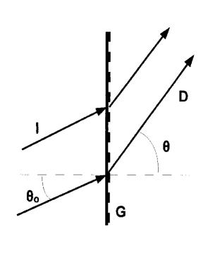
A plane wave of monochromatic light of frequency is incident at an angle on a plane (transmission) diffraction grating , with a spacing between grooves. The complex amplitude diffracted at a large distance from the grating, and at an angle from the normal to the plane of the grating is given by,
| (3) |
where,
| (4) |
with the wave length corresponding to , and we have omitted an overall factor , with a constant. is the total number of grooves illuminated by the incident plane wave, depends on the shape of the grooves, but does not depend on , and is, in general, slowly dependent on .
Let us assume for simplicity that . Then, the intensity of the diffracted light in the direction , , can be written as,
| (5) |
For large , (and fixed and ), this intensity has sharp maxima with for , such that,
| (6) |
where is a positive or negative integer, or,
| (7) |
Similarly, the intensity vanishes for , such that,
| (8) |
where is a positive or negative integer.
Restricting to , and calling the change in from the maximum to the closest zero, we have,
| (9) |
This can also be written as,
| (10) |
Suppose now we have a second normally incident monochromatic plane wave of frequency , and wavelength . The diffracted intensity will then be given by,
| (11) |
and there will be a maximum of for . If we define , and , we then have,
| (12) |
If we apply the criterion that the maxima for and for are seen as separate if the maximum of coincides with the closest zero of , we have that must be equal to of (10), and therefore,
| (13) |
This relation defines the resolving power of the grating. Typically, can be of the order of (or higher), so that one can resolve wavelengths , and that differ on the order of one part in (or more).
But here we want to consider this set up from a different point of view. We first notice that for a monochromatic wave we have,
| (14) |
where is the speed of propagation of the wave in the direction considered.
Suppose now the source of the monochromatic plane wave has a given, fixed frequency , and that we point the whole set up in different directions in space, while keeping the dimensions, relations and relative orientations of its different components (source, grating, supports, etc.) fixed. Notice that in (14) corresponds to what is called the one way speed of light, as no closed loops are involved. For fixed , and the rest of the parameters of the set up, a change in with the direction in which the set up points, will result in a change in , and, as a consequence, in the diffraction angle . Therefore, the set up will be sensitive to a possible dependence of on the direction of propagation, and thus provide a test of the isotropy of the one way speed of light. How sensitive can this set up be? In accordance with (13) and (14), and assuming that the same criterion is applicable, we would have that a negative result (no observable change in ), would indicate,
| (15) |
But, in deriving and applying (13) it was implicitly assumed that the sources of , and were incoherent. As we shall indicate in the next section, where we propose our basic idea for testing the isotropy of the one way speed of light, this can be very different when we consider a superposition of coherent plane waves.
III The basic idea
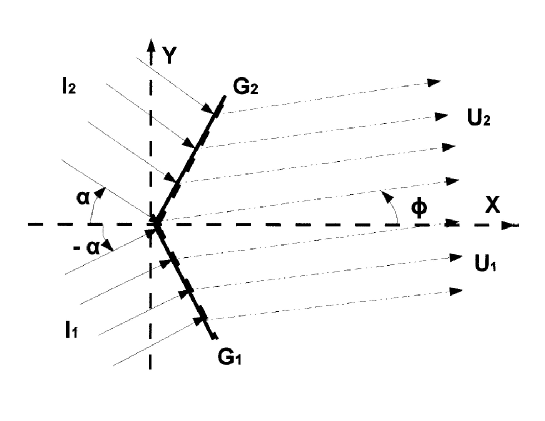
To clarify the basic idea, we refer to Figure 2, where we indicate the plane of an auxiliary orthogonal coordinate system with axes . The axis is perpendicular to the plane. Two identical plane transmission diffraction gratings, , and are placed with their grooves parallel to the axis, with one of their ends touching at the origin of coordinates. The planes of the gratings are set at angles , and respectively to plane. Two monochromatic, coherent, plane waves, , and , are normally incident respectively on , and , giving rise to diffracted amplitudes , and . The total diffracted amplitude, resulting from the superposition of and is to be observed at a large distance in the direction indicated by the angle .
In what follows we will only consider the case close to (and close to ). We have on this account, and for simplicity, set , as they are, in general, slowly changing factors, depending only on the angles and respectively. We have also dropped the factor , but have included a possible phase difference , between the two beams.
The resulting amplitude a long distance from the gratings, can now be computed as a function of the angle between the direction of the diffracted beams and the axis (see Figure 2). We have,
| (18) | |||||
and, therefore, the total amplitude as a function of , and is given by,
| (19) |
and the diffracted intensity is given by .
We are especially interested in the effect of changes in the wavelength on the pattern of diffracted light. Let us fix our attention on a particular wavelength . Define , and , for , and assume that the angle satisfies the relation,
| (20) |
so that for the maximum intensity of both diffracted beams corresponds to . For the condition (20) implies that in the direction we have,
| (21) |
We consider now the two extreme cases , and .
In the first case, (), for close to , we have,
| (22) |
This implies that the second term on the right of (22) will be of the same order as the first for , and, therefore, we expect that this will be also the order of the minimum observable difference . This is similar to the case of two incoherent beams.
In the second case, (), for close to , we have,
| (23) |
But now we have that for , and that for the first term in (23) will be of order one, while the second is of order . Therefore, in the case , the intensity at increases quadratically from zero to order one as increases from zero to order . This would indicate that in this case we have a much larger sensitivity to changes in , and corresponding changes in , than in the case of incoherent differences in wavelength. In the next Section we consider several examples to illustrate these points.
IV Some examples.
In the previous Section we considered only the intensities for . In this Section we consider several explicit examples, where we assume that the source has a unique, highly stable frequency, assign definite values to the grating parameters, and compute the intensities as a function of , for different choices of , and of . Our choice of parameters is: , , Å, and we also take Å, in correspondence with (20). The results are shown in several plots.
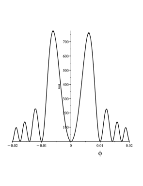
IV.1 The case
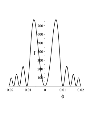
We consider first the case . In Figure 3, we have plots of the intensity as a function of for , (solid curve), , (dashed curve) and (dotted curve). Although the dotted curve, (), shows a clear separation of the maxima, we notice that already for the dashed curve, i.e. for , the maximum of the intensity has decreased to about half of that for . In fact, although not shown in Figure 3, we already have a decrease in the maximum of about , for , so that we may consider that in this case we have a resolution of the order of . We should also keep in mind that, for this choice of parameters, the maximum intensity is of the order of , and that the width of the diffracted line, taken as the angular separation between the zeros next to the maximum, is about .
In the next Subsection we consider the other extreme case, namely .
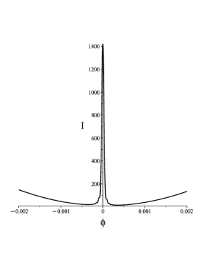
IV.2 The case
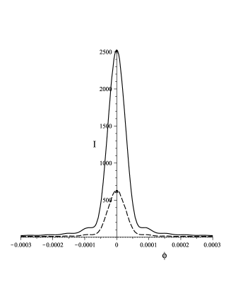
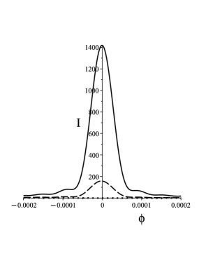
In the case , and for , we have complete cancellation of the diffracted amplitude only for . For , there is, in general, a non vanishing intensity as shown in Figure 4. We notice, however, that the first maximum of the diffracted intensity at either the right or left of , (with an intensity of the order of , i.e., five orders of magnitude below that for , and ), occur at , that is, at an angular separation about times the width of the diffracted line for (notice that the plot extends from to ). Thus, in the case , we have, around , a region much larger than the width of the diffracted line, where the intensity for can be taken as, essentially, zero. This is the situation depicted in Figure 5, which is restricted to the range .
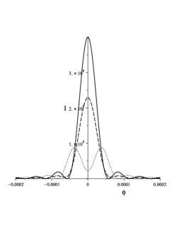
In Figure 5 we have a plot of the intensity as a function of in the range for several choices of . In accordance with the previous discussion, the curve corresponding to , plotted as a dotted line, can barely be distinguished from the horizontal axis, corresponding to . The dashed line corresponds to , and the solid line to . We can see that in this case the arrangement displays a sensitivity to changes in , and, therefore in , of the order of 1 part in . This, however, requires rather accurately. In the next Subsection we consider a value of close to but not equal to .
IV.3 The cases , but with close to .
Consider again (19), with , and satisfying condition (20). Expanding in up to order , after some simplifications, and keeping in each term the leading order in , we arrive at the following expression,
where,
| (25) | |||||
In the case (IV.3) reduces to,
| (26) |
so that, as already indicated, for the intensity has a maximum of intensity, in this case, of the order of , while for the first two terms on the right of (IV.3) (of order and , respectively) have vanishing coefficients, and we are left with,
| (27) |
We notice, however, that for , an effective cancellation of the first term on the right of (IV.3) would require that be of the order of or less, which, in turn, requires of the order of or less. On this account we consider now what happens for close to , but such that the first term in (IV.3) is still dominant.
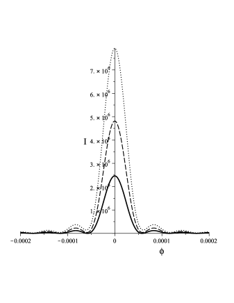
As a first example we chose the value which, on account of the previous discussion, is rather far from the value required for complete cancellation of the leading terms in (IV.3). The resulting intensities are shown in Figure 6 for several choices of . It is clear from this plot that already for there is a substantial change in the intensity.
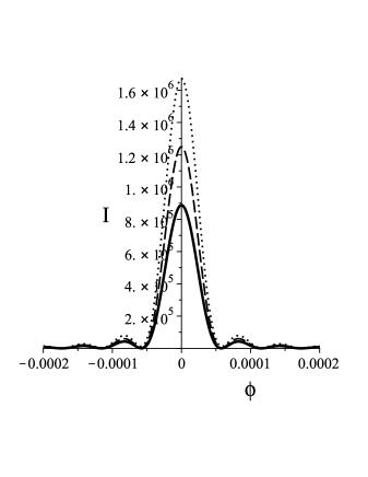
As a second example we considered . The results are shown in Figure 7. This, as expected, shows a higher sensitivity to changes in . In fact, already for we see a change of about in the line intensity.
We close this Section mentioning, although we do not provide explicit examples, that an increase in results also in an increase in sensitivity of the setup. In fact definitive numbers should better refer to a particular experimental arrangement. In the next Section we sketch, but only as an illustrative example, a possible arrangement, without entering in any constructive detail.
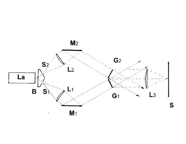
V An experimental setup
A possible basic setup for an experiment using the previous results can be described as follows (see Figure 8). We first assume an auxiliary orthogonal coordinate system with axes , (not shown in the figure), with X and Y in the plane of the figure, and Z perpendicular to that plane, and place a frequency stabilized laser ( in the figure) at the origin of coordinates. The laser emits monochromatic light along the axis. An artifact, , splits the laser light into two equal but separate beams that are directed to slits , and . A pair of lenses , and , situated in such a way that the slits are in their focal plane, transform the beams emerging from the slits into two plane waves. These are reflected on mirrors , and , so that they eventually arrive at the gratings , and , that have their grooves parallel to the direction Z, exactly in the form indicated in Figure 2, so that the previous discussion and results apply to the emerging diffracted light. The corresponding Fraunhoffer pattern can then be observed on the screen , in the focal plane the lens . The whole apparatus could be set on a platform, so that it can be oriented in different directions. Several comments are in order regarding this setup. The arrangement should include (not shown in Figure 8) some way of controlling both the amplitude and the phase of the beams in their way to the gratings , and . This can be achieved in different ways, and we have left it out for clarity. Regarding a concrete setup, besides the usual precautions, such as vibration isolation, a main concern would be temperature control, because a change in temperature, through temperature dilation, would result in a change in , and this is equivalent to a change in . Similar regards concern mechanical stability, because changes in the dimensions could introduce changes in the paths of light previous to the diffraction gratings, and this, in turn, changes in and the angle . It would also be appropriate to enclose the apparatus in a vacuum, and isolate it from electromagnetic disturbances.
In all this discussion we had in mind transmission diffraction gratings, but similar results would be obtained with reflective gratings, although the setup would be different.
VI Comments
In this note we have considered the problem of measuring the one way speed of light, taking into account the wave nature of light. For a monochromatic beam of light, propagating in a vacuum, this speed can be taken as the phase velocity, , where is the wavelength and the period. As remarked already, these quantities can be measured independently. The period by a local clock which that does not involve any type of synchronization, and by measuring the diffraction pattern generated as light passes through some known fixed structure, with no measurement of time or distance involved. We showed that although with an appropriate structure, such as a diffraction grating, one can measure with a certain precision, we can use the properties of the diffraction gratings as regards wavelengths, to construct a setup that is sensitive to changes in wavelength, which, for fixed , amounts to changes in , to a much greater accuracy than that obtained by direct measurement of .
The setup that we have considered can then be viewed as providing the basis for a null type experiment, where one checks for possible changes in the diffraction pattern as the apparatus is made to point in different directions. The invariance of the diffraction pattern (null result) would then provide an upper bound on the possible anisotropy of the one way propagation of light. As shown here, this upper bound could be on the order of 1 part in . Combining these results with the known bounds on the isotropy of the two way speed of light, which are much smaller than this, we would immediately obtain a value of the one way speed of light, with the same accuracy of the order of one part in .
On the other hand, a definite non null result would establish the presence of an anisotropy in the one way speed of light, with an accuracy in the order of a few meters per second, whose origin and properties would certainly require much further analysis, both from the theoretical as from the experimental side.
Acknowledgments
I am grateful to Eli Yudowsky for bringing the question of the one way speed of light to my attention.
References
- [1] See for instance the review [2]. It is not our purpose here to add to this debate, rather, we will concentrate on the topic suggested by the title of this note.
- [2] R. Anderson, I. Vetharaniam, G.E. Stedman, Physics Reports 295 93 (1998).
- [3] See, for instance, M. Born and E. Wolf, Principles of optics, (Pergamon Press Oxford, England, 1986).
Appendix A A (slightly) more general setup.
In all the discussion in the text we have assumed equal amplitudes for the diffracted beams, as well as equal number of grooves () and equal groove separation (). This led rather naturally in the case to the total cancellation of the amplitude for , as well as to a small value of the amplitude in an appropriate neighborhood of .
In this Appendix we consider a slightly more general case, where we allow for different values of amplitudes, and for the gratings. We therefore write the total amplitude in the form,
| (28) |
with the intensity given by,
| (29) |
We fix now the angles imposing the condition that for , the maxima of the corresponding diffracted beams occur for :
| (30) | |||||
| (31) |
where,
| (32) | |||||
We are particularly interested in the behaviour of for and , near . To second order in we find,
Therefore, the intensity will vanish for and only if we impose:
| (34) |
If, assuming now (34) and , we expand the intensity to order , we find,
The term of order vanishes already for . The vanishing of the terms in and for would require,
| (36) |
but this cannot be satisfied in general for integer values of and . Nevertheless, we may impose that, for integer values of and , the left hand side of (36) be a good numerical approximation to the right hand side of (36). We shall assume that and have been chosen that way.
It is also interesting to see the general behaviour of the intensity for , and . Assuming again (34) and , we get,
| (39) |
which reduces to (23) for .
The derivations in this Section indicate that with appropriate fixing of the relative amplitudes () and number of grooves illuminated (), we essentially recover the results obtained in the main text, regarding the properties of the total diffracted intensity in the case . In the next Section we consider an explicit numerical example to illustrate this points.
Appendix B A numerical example
In this Section we shall consider as an explicit example, for , the case where Å, and Å. We also take Å.
Next we consider (36), which in this reads,
| (40) |
Then, taking, for instance, , if choose we have,
| (41) |
Taking this into account, we choose , and , set and replace all numerical values in (31) and (32). Using the resulting expression we compute for several choices of . In Figure 9 we have plot of as a function of for , and , in the range , which shows that this case of can be made essentially equal to the case of by appropriate choices of and . In an experimental set up this means controlling the amplitudes of the beams previous to the gratings, and controlling the extent of the gratings illuminated by those beams.
In Figure 10 we have a plot of the intensity for several values of , in the range . The solid curve, which shows a clear departure from the case , corresponds to , that is , although this departure is apparent already for (the dashed curve). The case is also shown in the figure as the dotted curve, barely distinguishable from the axis .
In Figure 11, mainly for clarity, we show a plot of the case of Figure 10, but here in the range , that is ten times that of Figure 10, to show the clear separation of this “signal” from the “background” .