Insights into regression-based cross-temporal forecast reconciliation
Abstract
Cross-temporal forecast reconciliation aims to ensure consistency across forecasts made at different temporal and cross-sectional levels. We explore the relationships between sequential, iterative, and optimal combination approaches, and discuss the conditions under which a sequential reconciliation approach (either first-cross-sectional-then-temporal, or first-temporal-then-cross-sectional) is equivalent to a fully (i.e., cross-temporally) coherent iterative heuristic. Furthermore, we show that for specific patterns of the error covariance matrix in the regression model on which the optimal combination approach grounds, iterative reconciliation naturally converges to the optimal combination solution, regardless the order of application of the uni-dimensional cross-sectional and temporal reconciliation approaches. Theoretical and empirical properties of the proposed approaches are investigated through a forecasting experiment using a dataset of hourly photovoltaic power generation. The study presents a comprehensive framework for understanding and enhancing cross-temporal forecast reconciliation, considering both forecast accuracy and the often overlooked computational aspects, showing that significant improvement can be achieved in terms of memory space and computation time, two particularly important aspects in the high-dimensional contexts that usually arise in cross-temporal forecast reconciliation.
-
Keywords
Coherent forecasts; Cross-temporal forecast reconciliation; Sequential, iterative, and optimal combination approaches
1 Introduction
A large number of observed phenomena require accurate forecasts across different dimensions, e.g., different time periods and granularities, geographical regions, customer groups. Achieving coherent forecasts at any level of (dis)aggregation is challenging but crucial for optimal decision making, resource allocation and operational efficiency. As effective decision making depends on the support of accurate and coherent forecasts, forecast reconciliation, originally intended as a specific tool to improve the accuracy of the forecasts of a hierarchical time series (Fliedner,, 2001; Hyndman et al.,, 2011; Wickramasuriya et al.,, 2019), has then become a key post-forecasting process aimed at improving the accuracy of forecasts for general linearly constrained multiple time series, of which hierarchical and grouped time series are a specific special case (Panagiotelis et al.,, 2021; Girolimetto and Di Fonzo, 2024b, ). The need for reconciliation arises when base forecasts of the components of a multivariate variable, often produced independently by separate organizational units or using different models, do not match the internal constraints applicable to that variable (Kourentzes,, 2022).
Classical reconciliation methods for hierarchical time series, such as bottom-up and top-down, have been widely employed to address cross-sectionally incoherent forecasts. However, as Pennings and van Dalen, (2017) point out, these classical methods frequently overlook valuable information from different levels of the hierarchy. The introduction of regression-based reconciliation techniques in recent years has addressed this limitation. Consequently, hierarchical forecasting has significantly evolved to include modern least squares-based reconciliation techniques in the cross-sectional framework (Hyndman et al.,, 2011; Wickramasuriya et al.,, 2019; Panagiotelis et al.,, 2021), which were later extended for temporal hierarchies (Athanasopoulos et al.,, 2017; Yang et al., 2017b, ; Spiliotis et al.,, 2019; Nystrup et al.,, 2020; Bergsteinsson et al.,, 2021; Nystrup et al.,, 2021). The temporal coherence aspect is a natural extension, requiring the reconciliation of forecasts with different time granularities, such as months, quarters, or years, to ensure consistency (Athanasopoulos et al.,, 2017).
The cross-temporal framework combines cross-sectional and temporal dimensions to achieve fully coherent forecasts (Kourentzes and Athanasopoulos,, 2019; Yagli et al.,, 2019; Punia et al.,, 2020; Spiliotis et al.,, 2020). In this setting, complexity and dimensions of the problem grow very quickly along with the requested computational time and memory. Kourentzes and Athanasopoulos, (2019) and Yagli et al., (2019) both tackle this issue using sequential procedures that alternate uni-dimensional reconciliation approaches. On the other hand, Di Fonzo and Girolimetto, 2023a proposed an iterative heuristic, extending the results so far, and an optimal (in the least squares sense) cross-temporal forecast reconciliation approach, that simultaneously encompasses both contemporaneous and temporal coherency.
In recent years, there has been a significant increase in the application of cross-temporal reconciliation techniques to improve the accuracy of forecasting models by addressing inconsistencies across different time horizons. Notable applications of these methods include the works of Sanguri et al., (2022), Di Fonzo and Girolimetto, 2023b , English and Abolghasemi, (2024), Quinn et al., (2024). Moreover, Girolimetto et al., (2024) proposed a probabilistic cross-temporal linear reconciliation technique, offering a more flexible approach to consider forecast uncertainties. Finally, it is worth mentioning the contribution by Rombouts et al., (2024), who recently proposed the first Machine Learning-based cross-temporal forecast reconciliation technique, and performed an empirical comparison with the standard linear approaches.
In this paper, we address some open-issues related to the relationships between sequential, iterative and optimal combination cross-temporal forecast reconciliation approaches. We discuss the conditions under which a sequential (either first-cross-sectional-then-temporal, or first-temporal-then-cross-sectional) approach, is equivalent to a fully (i.e, cross-temporally) coherent iterative heuristic. We also show that, for specific patterns of the error covariance matrix of the regression model on which the optimal combination approach grounds, an iterative reconciliation procedure ‘converges’ to the optimal combination reconciliation solution regardless the order with which each uni-dimensional reconciliation is applied. The reduction of the computing effort is evaluated in the experiment of forecasting hourly photovoltaic power generation considered by Yagli et al., (2019) and Di Fonzo and Girolimetto, (2022); Di Fonzo and Girolimetto, 2023b .
The paper is organised as follows. In Section 2, we briefly recapitulate the main definitions and results for cross-sectional, temporal and cross-temporal forecast reconciliation, following the notation presented in Athanasopoulos et al., (2024) and extended in Girolimetto et al., (2024). In Section 3, we present two new results, in the form of theorems describing the relationships between sequential, iterative and optimal cross-temporal reconciliation approaches. To assess the impact of the new results on memory space and computation time, a forecasting experiment on an hourly power generation dataset is presented in Section 4. Conclusions follow in Section 5. All the forecast reconciliation procedures considered in this paper are available in the R package FoReco (Girolimetto and Di Fonzo, 2024a, ).
2 Regression-based cross-temporal reconciliation
In this section, we briefly describe the optimal combination cross-temporal point forecast reconciliation methodology (Di Fonzo and Girolimetto, 2023a, ), and the different regression-based heuristic approaches proposed by Yagli et al., (2019), Kourentzes and Athanasopoulos, (2019), and Di Fonzo and Girolimetto, (2022); Di Fonzo and Girolimetto, 2023a ; Di Fonzo and Girolimetto, 2023b . For more details, the reader is referred to the original articles. The extension to the probabilistic forecast reconciliation setting, which is beyond the scope of this paper, may be pursued according to Girolimetto et al., (2024).
Let be the matrix containing the values to be forecasted of a linearly constrained -variate time series for all the temporal aggregation orders (e.g., for a quarterly time series, , where corresponds to the annual frequency, semi-annual, and quarterly, wich is the highest observed frequency) where and . Matrix can be written as:
where , , is the matrix containing the target values of the temporally aggregated series of order . The variables are split into a matrix and a matrix . These matrices represent, respectively, the upper () and bottom () level variables at any temporal aggregation order within the cross-sectional hierarchy, where the total number of variables is given by . It is worth noting that in the cross-temporal framework, the ‘very bottom’ variables are the highest-frequency bottom time series in matrix .
| Regression-based reconciliation: structural representation | Constraints | |||
| Matrix form | Vector form | Reconciled | cs | te |
| yes | no | |||
| no | yes | |||
| yes | yes | |||
Now, we denote and the structural (summing) matrices in the cross-sectional and temporal frameworks, respectively, mapping the relevant bottom variables into their complete counterpart vector. The structural representations valid for all variables and all temporal aggregation orders , which take into account either cross-sectional or temporal coherence, are given by and , respectively. Since , and , we can express in matrix form the cross-temporal structural representation as well: . Moreover, it is convenient to consider the vectorized forms of the structural representations above:
where , , , , and
with the cross-temporal structural matrix, encompassing both contemporaneous and temporal constraints. The results shown so far are summarized in Table 1 along with the expression for the reconciled forecasts through the classical formula (Hyndman et al.,, 2011):
| (1) |
with , where is a base forecasts’ error covariance matrix for the entire system of involved variables, at any cross-sectional and temporal aggregation levels, and are oblique projection matrices (Panagiotelis et al.,, 2021). More precisely, is the oblique projection in the space spanned by the columns of , and is the oblique projection in the space spanned by the columns of . In addition, is the oblique projection in the space , given by the intersection of and (i.e., ), spanned by the columns of . These three approaches are optimal in the least squares sense, but only is cross-temporally coherent.
In addition to the structural representation, forecast reconciliation can be formulated as a linear constrained quadratic program (Stone et al.,, 1942; Byron,, 1978, 1979; Solomou and Weale,, 1993; Di Fonzo and Girolimetto, 2023a, ), as described in Table 2, starting from the zero-constrained representation
where and denote the zero-constraints matrices representing the relationships between the variables in cross-sectional and temporal frameworks, respectively. Also in this case, we may consider the vectorized forms of the constraints:
where
and
is the cross-temporal matrix encompassing both contemporaneous and temporal constraints.
| Regression-based reconciliation: zero-constrained representation | Constraints | |||
| Matrix form | Vector form | Reconciled | cs | te |
| yes | no | |||
| no | yes | |||
| yes | yes | |||
We can express the reconciled forecasts through the formula proposed by Stone et al., (1942) (Byron,, 1978, 1979; Di Fonzo and Girolimetto, 2023a, ),
| (2) |
where is a projection matrix. The formulae to compute and have been used by Yagli et al., (2019) in two heuristic sequential reconciliation approaches, respectively called cross-sectional-then-temporal (cst) and temporal-then-cross-sectional (cts, see Di Fonzo and Girolimetto, 2023a, ), given by:
where the forecasts in () are not cross-sectionally (temporally) coherent.
Theorem 1 in Section 3 establishes sufficient conditions under which the equality holds. Furthermore, it is shown that under the same conditions, is equivalent to an optimal combination cross-temporal forecast reconciliation solution with a specific error covariance matrix.
A second heuristic proposed by Kourentzes and Athanasopoulos, (2019) is able to obtain cross-temporally coherent forecasts starting from either of the two sequential approaches so far. In particular, the technique consists in an ensemble forecasting procedure that exploits the simple averaging of different forecasts:
with
where is the cross-sectional projection matrix for each temporal aggregation order and is the temporal projection matrix for each single variable (see Di Fonzo and Girolimetto, 2023a, ).
Finally, Di Fonzo and Girolimetto, 2023a proposed an iterative cross-temporal reconciliation approach alternating forecast reconciliation along one single dimension (cross-sectional or temporal) in a cyclic fashion, until a convergence criterion is met:
It is worth noting that, provided convergence was achieved in both cases, and are cross-temporally coherent, but in general .
3 Two new results
The first result (Theorem 1) shows that if the error covariance matrices used in either steps of an iterative reconciliation approach are constant across levels and time granularities, (i) fully reconciled forecasts are obtained in a single (two-step) iteration, (ii) the final result does not depend on the order of application of the uni-dimensional reconciliation approaches, and (iii) the solution is equivalent to that obtained through an optimal combination approach using a separable covariance matrix with a Kronecker product structure.
Theorem 1.
Let , , , be the cross-sectional hierarchy error covariance matrix, and , , the error covariance matrix for the -th series temporal hierarchy. If , and , and , , then:
-
1.
the iterative cross-temporal forecast reconciliation approach reduces to a single (two-step) iteration. Furthermore, , where () is the [] matrix of the temporal-then-cross-sectional (cross-sectional-then-temporal) reconciled forecasts;
-
2.
the heuristic cross-temporal reconciliation approach by Kourentzes and Athanasopoulos, (2019) is equivalent to a sequential approach;
-
3.
denoting the optimal combination reconciled forecasts obtained by using the covariance matrix , it is .
Proof.
-
1.
If , and , and , , the cross-sectional and temporal reconciled forecasts are respectively given by , and , where and are the and , respectively, oblique projection matrices
It easy to check that . In addition, as both and are cross-temporally coherent, it is .
-
2.
Under the conditions of the theorem we have: and . It follows that
and then
-
3.
Recalling that , after a few algebraic steps we find that the optimal combination cross-temporal reconciled forecasts may be expressed as:
On the other hand, as and , it follows
∎
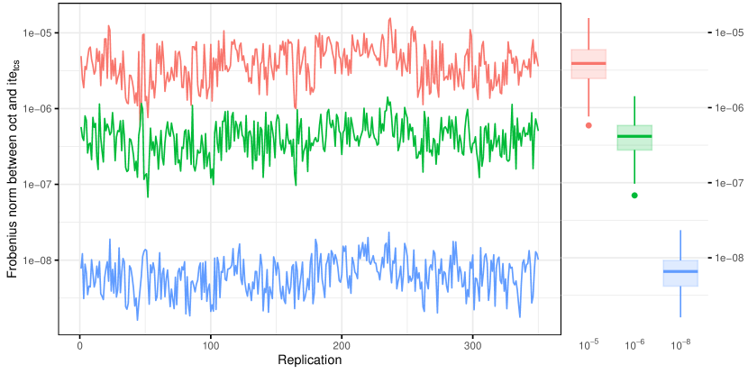
In general, when an iterative reconciliation procedure ‘converges’ to an optimal combination reconciliation approach, this happens regardless the order with which each uni-dimensional reconciliation is applied. A well-known example is the iterative approach where the diagonal covariance matrices computed using the one-step-ahead in-sample forecast errors are used in the cross-sectional phase, and the diagonal matrix “which contains estimates of the in-sample one-step-ahead error variances across each level” (Athanasopoulos et al.,, 2017, p. 64) in the temporal one. Figure 1 shows the Frobenius norm of the difference between the reconciled forecasts obtained through the optimal (with cross-temporal series variance scaling covariance) and iterative heuristic (alternating the temporal series variance scaling and the cross-sectional series variance reconciliation approaches) formulae. The convergence is shown based on 350 replications of the forecasting experiment detailed in Section 4, with different convergence tolerance levels ( in red, in green, and in blue). We obtain similar results using .
These empirical observation is theoretically justified by Theorem 2, that presents a sufficient condition under which an iterative reconciliation heuristic converges to an optimal combination approach.
Theorem 2.
Let , , be the cross-sectional hierarchy error covariance matrix with , and , , the -th series temporal hierarchy error covariance matrix with , with the commutation matrix operating on matrices of dimension (e.g., ), such that . If , then the iterative reconciled forecasts converge in norm to the optimal combination reconciled forecasts with cross-temporal covariance matrix .
Proof.
Let and be the matrix of the temporal-then-cross-sectional and cross-sectional-then-temporal iterative reconciled forecasts using () and () as the cross-sectional and temporal covariance matrices, respectively. The iterative solution obtained at a given complete recursion , may be written as the result of alternating oblique projections, such that , with
| (3) |
We want to prove that .
Since , where is p.d., we can express its inverse as , where is a (unique) upper triangular matrix with positive diagonal elements. Thus, denoting , it can be shown that
where , with , , and , with . Matrices , are orthogonal projection matrices onto the linear sub-spaces spanned by the columns of, respectively, , , and . The oblique projection matrices (3) can thus be written using the orthogonal projection matrices , , such that . As , it follows
As the alternating orthogonal projections onto two subspaces converges in norm to the projection onto the intersection of the two subspaces111Thanks to Tommaso Proietti for suggesting considering alternating projections., we have . The convergence of to is easily obtained by inverting the order in which matrices and are applied in the proof. ∎
4 Empirical application
The dataset PV324 (Yang et al., 2017a, ; Yang et al., 2017b, ; Yagli et al.,, 2019; Di Fonzo and Girolimetto,, 2022; Di Fonzo and Girolimetto, 2023b, ) refers to simulated data from 318 photovoltaic (PV) plants located in California. The hourly irradiation data from these PV plants are structured into three hierarchical levels to facilitate various aggregation analyses (Figure 2).
At the highest level, , there is a single time series representing the total irradiation data for the Independent System Operator (ISO), which is derived by summing the irradiation data from all 318 PV plants. The intermediate level, , consists of five time series, each representing one of the Transmission Zones (TZ) within California. These TZ time series are aggregated from groups of 27, 73, 101, 86, and 31 PV plants, respectively. At the most granular level, , there are 318 time series, each corresponding to the hourly irradiation data of an individual PV plant.
To assess the new results presented so far, we consider the forecasting experiment pursued by Di Fonzo and Girolimetto, 2023b aligned with the operational forecasting requirements of the public corporation managing power grid operations in California (CAISO, Makarov et al.,, 2011; Kleissl,, 2013), ensuring that the experiment closely mimics real-world conditions for grid management and power forecasting operations222A complete set of results is available at the GitHub repository https://github.com/danigiro/ct-comp.. The forecasts were generated with a rolling window of 14 days (336 hours) as training set for a horizon of two days (48 hours), with a specific focus on evaluating the performance of the day 2 (operating day). The base forecasts for the 318 plant-level () time series were derived from numerical weather prediction (NWP) forecasts provided by 3TIER (3TIER,, 2010). For the six aggregated time series at and levels and for the time series at various temporal aggregations (2, 3, 4, 6, 8, 12, and 24 hours), the exponential smoothing state space model (ETS) from the R-package forecast (Hyndman et al.,, 2021) was employed to generate the base forecasts. We consider a total of 3 benchmarks:
-
NWP forecasts for the 318 plant-level time series and ETS for all the aggregated series;
-
PERS
the forecast at any given hour is equal to the observed value at same hour on the previous day and the forecasts for any temporal granularity are obtained through cross-temporal bottom-up;
-
3TIER
the NWP forecasts provided by 3TIER are used for the hourly aggregated level, cross-temporal bottom-up is used for all the other levels.
Standard forecast reconciliation techniques can sometimes result in negative values. This is problematic when dealing with variables that are naturally non-negative, like PV power generation, as negative values are illogical in such scenarios. The set-negative-to-zero (sntz) approach proposed by Di Fonzo and Girolimetto, 2023b is used to avoid this issue. In Figure 3, we compare computational times and CPU memory allocation across iterative ( and ), optimal (), or heuristic (ka and ka) approaches, in the following cases:
-
and with and equivalent to with (Theorem 1);
-
and with and equivalent to and with (Theorem 1);
-
and with and equivalent to with (Theorem 1);
-
and with and equivalent to with (Theorem 1);
-
and alternating temporal series variance scaling and cross-sectional series variance reconciliation approaches, and using the cross-temporal series variance scaling covariance. Following Theorem 2, converges to .
Specifically, Figures 3(a) and 3(b) show the computational performance of the forecasting experiment over 350 replications. Figure 3(a) illustrates the computational times, measured in seconds, required for each approach, while Figure 3(b) shows the corresponding CPU memory usage in megabytes. In both figures, each panel represents a different reconciliation approaches, with the techniques displayed along the y-axes for comparison.
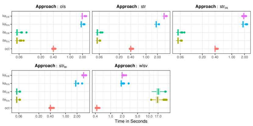
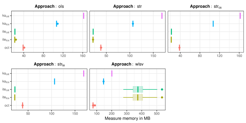
In agreement with Theorem 1, , , , and give identical reconciled forecasts. When using , both iterative heuristics converge to the optimal solution, as stated by Theorem 2, while the KA heuristics ( and ) do not. In details, the iterative approaches with a single iteration (, , , and ) are faster and use less memory than all other methods. However, when the number of iterations exceeds 1 (), it becomes the most expensive in terms of both CPU memory and time. Overall, the empirical evidence highlights a clear advantage of the optimal approach, emphasizing its computational efficiency and practical suitability compared to the equivalent KA heuristics. The same result holds for the optimal approach when compared to the corresponding iterative heuristic.
| Temporal aggregation orders | ||||||||
| App. | ||||||||
| PERSbu | 34.62 | 34.14 | 33.35 | 33.11 | 29.45 | 32.23 | 20.83 | 20.23 |
| 3TIERbu | 26.03 | 25.34 | 24.56 | 23.31 | 22.09 | 19.89 | 15.70 | 12.48 |
| 27.85 | 27.55 | 28.31 | 29.69 | 28.01 | 35.32 | 21.04 | 18.17 | |
| 30.15 | 29.40 | 28.05 | 28.41 | 24.87 | 27.66 | 17.71 | 17.22 | |
| 26.64 | 26.27 | 25.56 | 25.48 | 22.86 | 24.71 | 16.25 | 15.73 | |
| 28.18 | 27.76 | 27.01 | 26.91 | 24.05 | 26.14 | 17.06 | 16.56 | |
| 28.53 | 28.02 | 26.98 | 27.18 | 24.07 | 26.44 | 17.14 | 16.64 | |
| 23.63 | 23.18 | 22.55 | 22.32 | 20.16 | 21.40 | 14.30 | 13.64 | |
| katcs | 23.63 | 23.06 | 22.43 | 22.19 | 20.04 | 21.25 | 14.23 | 13.55 |
| kacst | 24.21 | 23.77 | 23.14 | 22.94 | 20.70 | 22.05 | 14.66 | 14.03 |
| PERSbu | 43.15 | 42.42 | 41.27 | 40.81 | 36.29 | 39.19 | 25.66 | 24.57 |
| 3TIERbu | 33.95 | 32.94 | 31.90 | 30.62 | 28.02 | 26.99 | 19.87 | 16.75 |
| 34.24 | 34.04 | 33.79 | 35.01 | 33.11 | 40.51 | 25.16 | 20.94 | |
| 38.19 | 36.98 | 34.83 | 35.38 | 30.72 | 34.05 | 21.80 | 20.94 | |
| 32.99 | 32.41 | 31.45 | 31.23 | 27.96 | 29.91 | 19.88 | 19.00 | |
| 35.02 | 34.38 | 33.31 | 33.09 | 29.52 | 31.76 | 20.94 | 20.05 | |
| 35.17 | 34.43 | 33.03 | 33.18 | 29.33 | 31.89 | 20.87 | 20.01 | |
| 30.21 | 29.52 | 28.66 | 28.27 | 25.40 | 26.79 | 18.02 | 17.01 | |
| katcs | 30.24 | 29.40 | 28.53 | 28.13 | 25.27 | 26.64 | 17.95 | 16.92 |
| kacst | 30.82 | 30.15 | 29.27 | 28.91 | 25.97 | 27.47 | 18.41 | 17.43 |
| PERSbu | 59.75 | 56.81 | 54.23 | 52.87 | 46.82 | 49.07 | 33.12 | 30.65 |
| 3TIERbu | 53.46 | 50.57 | 48.33 | 46.19 | 41.36 | 40.72 | 29.28 | 25.19 |
| 53.46 | 47.22 | 44.87 | 44.30 | 39.68 | 42.66 | 30.92 | 25.82 | |
| 50.69 | 47.64 | 44.66 | 44.53 | 38.86 | 41.71 | 27.64 | 25.82 | |
| 46.51 | 43.80 | 41.80 | 40.83 | 36.34 | 37.90 | 25.85 | 23.97 | |
| 47.95 | 45.27 | 43.22 | 42.26 | 37.55 | 39.38 | 26.67 | 24.81 | |
| 48.84 | 46.02 | 43.48 | 43.08 | 37.92 | 40.24 | 27.00 | 25.17 | |
| 44.44 | 41.52 | 39.63 | 38.43 | 34.27 | 35.25 | 24.35 | 22.27 | |
| katcs | 44.48 | 41.45 | 39.55 | 38.34 | 34.18 | 35.15 | 24.30 | 22.21 |
| kacst | 44.76 | 41.86 | 39.98 | 38.80 | 34.59 | 35.67 | 24.56 | 22.52 |
Following Yagli et al., (2019) and Di Fonzo and Girolimetto, 2023b , the accuracy of the considered approaches is measured in terms of normalized Root Mean Square Error (nRMSE):
where , denotes the series, , with , denotes the forecasting approach, and . In Table 3, we report the nRMSE at different cross-sectional (, and ) and temporal () levels. Note that we compare the optimal solution for all the approaches (, , , , ) as well as the results for ka and ka alternating the temporal series variance scaling and the cross-sectional series variance matrices. The PERS approach, used as a baseline, almost always has the highest nRMSE values. In contrast, the 3TIER and approaches demonstrate significant improvements over the base forecasts, especially at higher temporal aggregation orders, as discussed in Di Fonzo and Girolimetto, 2023b . and are always better than , but worse than . Notably, the and ka approaches yield the lowest nRMSE values, reflecting their superior forecasting accuracy across all cross-sectional levels and temporal aggregation orders.
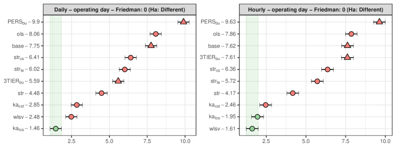
The Multiple Comparison with the Best (MCB) Nemenyi test (Koning et al.,, 2005; Kourentzes and Athanasopoulos,, 2019; Makridakis et al.,, 2022) allows to establish if the forecasting performances of the considered techniques are significantly different. This procedure shown in Figure 4 evaluates the accuracy of hourly and daily solar irradiation forecasts focusing on the operating day forecast horizon for all the 324 series across , , and levels. For daily forecasts, the approach is the most accurate, followed closely by ka and ka. The comparable performance of these three approaches is evident from their overlapping intervals, that means no statistically significant difference in their accuracy. On the other hand, approaches such as PERS, , and show worse performance compared to , as indicated by the non-overlapping intervals. For hourly forecasts, a similar trend emerges, with ka showing superior accuracy, immediately followed by and ka. However, the intervals of , ka, and ka slightly overlap, suggesting that their performances are statistically different. It should be noted that even if does not perform as well as the top three approaches, it consistently outperforms all the remaining approaches, including , PERS and 3TIER.
5 Conclusion
This paper investigates the relationships between sequential, iterative and optimal combination cross-temporal forecast reconciliation approaches. Our study establishes conditions under which a sequential approach, whether starting from a cross-sectional or temporal reconciliation, is equivalent to the heuristics proposed by Kourentzes and Athanasopoulos, (2019) and Di Fonzo and Girolimetto, 2023a . We found that when error covariance matrices remain consistent across different levels and time granularities, these heuristics give the optimal combination approach solution that employs a separable covariance matrix based on the Kronecker product. Moreover, we demonstrate that specific patterns in the error covariance matrix of the iterative reconciliation converge to the optimal solution, regardless of the order of application of the uni-dimensional reconciliation steps. In addition, we offer a comprehensive framework for understanding and improving cross-temporal forecast reconciliation, taking into consideration not only the forecast accuracy, but also computational aspects that have so far been quite overlooked.
Our empirical application utilizes the PV324 dataset (Yagli et al.,, 2019), with 324 simulated hourly irradiation data from photovoltaic plants in California, structured into a three-level hierarchy. The experiment employs a rolling window forecasting approach with a 14-day training set and a two-day forecast horizon. The findings indicate that iterative approaches with a single iteration are computationally faster and utilize less memory compared to methods requiring multiple iterations. Moreover, the optimal combination approach demonstrates better trade-off between accuracy and computational efficiency compared to the two heuristics and the different benchmarks.
These results have significant implications for the field of time series forecasting, particularly in applications requiring high-dimensional and hierarchical forecast reconciliation. By highlighting the conditions under which different reconciliation techniques are equivalent, this research provides valuable insights for practitioners aiming to optimize forecasting accuracy and efficiency.
Future research could explore the application of these findings to other types of hierarchical structures and different domains, as well as the potential integration of machine learning techniques (Rombouts et al.,, 2024) to further enhance forecast reconciliation processes.
Acknowledgments
The authors thank all the participants to the 52nd Scientific Meeting of the Italian Statistical Society in Bari (Italy) and the 44th International Symposium on Forecasting in Dijon (France). Funding support for this article was provided by the Ministero dell’Università e della Ricerca with the project PRIN2022 “PRICE: A New Paradigm for High Frequency Finance” 2022C799SX.
References
- 3TIER, (2010) 3TIER (2010). Development of Regional Wind Resource and Wind Plant Output Datasets: Final Subcontract Report. Electricity generation, Energy storage, Forecasting wind, Solar energy, Wind energy, Wind farms, Wind modeling. (visited on October 16, 2024) https://digitalscholarship.unlv.edu/renew_pubs/4.
- Athanasopoulos et al., (2024) Athanasopoulos, G., Hyndman, R. J., Kourentzes, N., & Panagiotelis, A. (2024). Forecast reconciliation: A review. International Journal of Forecasting, 40(2), 430–456, https://doi.org/10.1016/j.ijforecast.2023.10.010.
- Athanasopoulos et al., (2017) Athanasopoulos, G., Hyndman, R. J., Kourentzes, N., & Petropoulos, F. (2017). Forecasting with temporal hierarchies. European Journal of Operational Research, 262(1), 60–74, https://doi.org/10.1016/j.ejor.2017.02.046.
- Bergsteinsson et al., (2021) Bergsteinsson, H., Møller, J. K., Nystrup, P., Pálsson, Ó. P., Guericke, D., & Madsen, H. (2021). Heat load forecasting using adaptive temporal hierarchies. Applied Energy, 292, https://doi.org/10.1016/j.apenergy.2021.116872.
- Byron, (1978) Byron, R. P. (1978). The estimation of large social account matrices. Journal of the Royal Statistical Society. Series A, 141(3), 359–367, https://doi.org/10.2307/2344807.
- Byron, (1979) Byron, R. P. (1979). Corrigenda: The estimation of large social account matrices. Journal of the Royal Statistical Society. Series A, 142(3), 405, https://doi.org/10.2307/2982515.
- Di Fonzo and Girolimetto, (2022) Di Fonzo, T. & Girolimetto, D. (2022). Enhancements in cross-temporal forecast reconciliation, with an application to solar irradiance forecasting. https://doi.org/10.48550/arXiv.2209.07146.
- (8) Di Fonzo, T. & Girolimetto, D. (2023a). Cross-temporal forecast reconciliation: Optimal combination method and heuristic alternatives. International Journal of Forecasting, 39(1), 39–57, https://doi.org/10.1016/j.ijforecast.2021.08.004.
- (9) Di Fonzo, T. & Girolimetto, D. (2023b). Spatio-temporal reconciliation of solar forecasts. Solar Energy, 251, 13–29, https://doi.org/10.1016/j.solener.2023.01.003.
- English and Abolghasemi, (2024) English, L. & Abolghasemi, M. (2024). Improving the forecast accuracy of wind power by leveraging multiple hierarchical structure. Sustainable Energy, Grids and Networks, 40, 101517, https://doi.org/10.1016/j.segan.2024.101517.
- Fliedner, (2001) Fliedner, G. (2001). Hierarchical forecasting: Issues and use guidelines. Industrial Management & Data Systems, 101(1), 5–12, https://doi.org/10.1108/02635570110365952.
- Girolimetto et al., (2024) Girolimetto, D., Athanasopoulos, G., Di Fonzo, T., & Hyndman, R. J. (2024). Cross-temporal probabilistic forecast reconciliation: Methodological and practical issues. International Journal of Forecasting, 40(3), 1134–1151, https://doi.org/10.1016/j.ijforecast.2023.10.003.
- (13) Girolimetto, D. & Di Fonzo, T. (2024a). Package FoReco: Forecast Reconciliation. Version 1.0. https://doi.org/10.32614/CRAN.package.FoReco.
- (14) Girolimetto, D. & Di Fonzo, T. (2024b). Point and probabilistic forecast reconciliation for general linearly constrained multiple time series. Statistical Methods & Applications, 33, 581–607, https://doi.org/10.1007/s10260-023-00738-6 https://doi.org/10.1007/s10260-023-00738-6.
- Hyndman et al., (2011) Hyndman, R. J., Ahmed, R. A., Athanasopoulos, G., & Shang, H. L. (2011). Optimal combination forecasts for hierarchical time series. Computational Statistics and Data Analysis, 55(9), 2579–2589, https://doi.org/10.1016/j.csda.2011.03.006.
- Hyndman et al., (2021) Hyndman, R. J., et al. (2021). Package forecast: Forecasting functions for time series and linear models. Version 8.15 https://pkg.robjhyndman.com/forecast/.
- Kleissl, (2013) Kleissl, J. (2013). Solar energy forecasting and resource assessment. London: Academic Press.
- Koning et al., (2005) Koning, A. J., Franses, P. H., Hibon, M., & Stekler, H. O. (2005). The M3 competition: Statistical tests of the results. International Journal of Forecasting, 21(3), 397–409, https://doi.org/10.1016/j.ijforecast.2004.10.003.
- Kourentzes, (2022) Kourentzes, N. (2022). Toward a one-number forecast: Cross-temporal hierarchies. Foresight: The International Journal of Applied Forecasting, 67, 32–40.
- Kourentzes and Athanasopoulos, (2019) Kourentzes, N. & Athanasopoulos, G. (2019). Cross-temporal coherent forecasts for Australian tourism. Annals of Tourism Research, 75, 393–409, https://doi.org/10.1016/j.annals.2019.02.001.
- Makarov et al., (2011) Makarov, Y. V., Etingov, P. V., Ma, J., Huang, Z., & Subbarao, K. (2011). Incorporating uncertainty of wind power generation forecast into power system operation, dispatch, and unit commitment procedures. IEEE Transactions on Sustainable Energy, 4(1), 433–442, https://doi.org/10.1109/TSTE.2011.2159254.
- Makridakis et al., (2022) Makridakis, S., Spiliotis, E., & Assimakopoulos, V. (2022). The M5 Accuracy competition: Results, findings and conclusions. International Journal of Forecasting, 38(4), 1346–1364, https://doi.org/10.1016/j.ijforecast.2021.11.013.
- Nystrup et al., (2021) Nystrup, P., Lindström, E., Møller, J. K., & Madsen, H. (2021). Dimensionality reduction in forecasting with temporal hierarchies. International Journal of Forecasting, in press, https://doi.org/10.1016/j.ijforecast.2020.12.003.
- Nystrup et al., (2020) Nystrup, P., Lindström, E., Pinson, P., & Madsen, H. (2020). Temporal hierarchies with autocorrelation for load forecasting. European Journal of Operational Research, 280(3), 876–888, https://doi.org/10.1016/j.ejor.2019.07.061.
- Panagiotelis et al., (2021) Panagiotelis, A., Athanasopoulos, G., Gamakumara, P., & Hyndman, R. J. (2021). Forecast reconciliation: A geometric view with new insights on bias correction. International Journal of Forecasting, 37(1), 343–359, https://doi.org/10.1016/j.ijforecast.2020.06.004.
- Pennings and van Dalen, (2017) Pennings, C. L. P. & van Dalen, J. (2017). Integrated hierarchical forecasting. European Journal of Operational Research, 263(2), 412–418, https://doi.org/10.1016/j.ejor.2017.04.047.
- Punia et al., (2020) Punia, S., Singh, S. P., & Madaan, J. K. (2020). A cross-temporal hierarchical framework and deep learning for supply chain forecasting. Computers & Industrial Engineering, 149, 106796, https://doi.org/10.1016/j.cie.2020.106796.
- Quinn et al., (2024) Quinn, C. O., Corliss, G. F., & Povinelli, R. J. (2024). Cross-temporal hierarchical forecast reconciliation of natural gas demand. Energies, 17(13), 3077, https://doi.org/10.3390/en17133077.
- Rombouts et al., (2024) Rombouts, J., Ternes, M., & Wilms, I. (2024). Cross-temporal forecast reconciliation at digital platforms with machine learning. International Journal of Forecasting, (in press), https://doi.org/10.1016/j.ijforecast.2024.05.008.
- Sanguri et al., (2022) Sanguri, K., Shankar, S., Punia, S., & Patra, S. (2022). Hierarchical container throughput forecasting: The value of coherent forecasts in the management of ports operations. Computers & Industrial Engineering, 173, 108651, https://doi.org/10.1016/j.cie.2022.108651.
- Solomou and Weale, (1993) Solomou, S. & Weale, M. (1993). Balanced estimates of national accounts when measurement errors are autocorrelated. Journal of the Royal Statistical Society A, 156(1), 89–105, https://doi.org/10.2307/2982862.
- Spiliotis et al., (2019) Spiliotis, E., Petropoulos, F., & Assimakopoulos, V. (2019). Improving the forecasting performance of temporal hierarchies. PLoS One, 14(10), e0223422, https://doi.org/10.1371/journal.pone.0223422.
- Spiliotis et al., (2020) Spiliotis, E., Petropoulos, F., Kourentzes, N., & Assimakopoulos, V. (2020). Cross-temporal aggregation: Improving the forecast accuracy of hierarchical electricity consumption. Applied Energy, 261, 114339, https://doi.org/10.1016/j.apenergy.2019.114339.
- Stone et al., (1942) Stone, R., Champernowne, D. G., & Meade, J. E. (1942). The precision of national income estimates. Review of Economic Studies, 9(2), 111–125, https://doi.org/10.2307/2967664.
- Wickramasuriya et al., (2019) Wickramasuriya, S. L., Athanasopoulos, G., & Hyndman, R. J. (2019). Optimal forecast reconciliation for hierarchical and grouped time series through trace minimization. Journal of the American Statistical Association, 114(526), 804–819, https://doi.org/10.1080/01621459.2018.1448825.
- Yagli et al., (2019) Yagli, G. M., Yang, D., & Srinivasan, D. (2019). Reconciling solar forecasts: Sequential reconciliation. Solar Energy, 179, 391–397, https://doi.org/10.1016/j.solener.2018.12.075.
- (37) Yang, D., Quan, H., Disfani, V. R., & Liu, L. (2017a). Reconciling solar forecasts: Geographical hierarchy. Solar Energy, 146, 276–286, https://doi.org/10.1016/j.solener.2017.02.010.
- (38) Yang, D., Quan, H., Disfani, V. R., & Rodríguez-Gallegos, C. D. (2017b). Reconciling solar forecasts: Temporal hierarchy. Solar Energy, 158, 332–346, https://doi.org/10.1016/j.solener.2017.09.055.