Calculation of heavy meson light-cone distribution amplitudes from lattice QCD

Abstract

We develop an approach for calculating heavy quark effective theory (HQET) light-cone distribution amplitudes (LCDAs) by employing a sequential effective theory methodology. The theoretical foundation of the framework is established, elucidating how the quasi distribution amplitudes (quasi DAs) with three scales can be utilized to compute HQET LCDAs. We provide theoretical support for this approach by demonstrating the rationale behind devising a hierarchical ordering for the three involved scales, discussing the factorization at each step, clarifying the underlying reason for obtaining HQET LCDAs in the final phase, and addressing potential theoretical challenges. The lattice QCD simulation aspect is explored in detail, and the computations of quasi DAs are presented. We employ three fitting strategies to handle contributions from excited states and extract the bare matrix elements. For renormalization purposes, we apply hybrid renormalization schemes at short and long distance separations. To mitigate long-distance perturbations, we perform an extrapolation in $\lambda=z\cdot P^{z}$ and assess the stability against various parameters. After two-step matching, our results for HQET LCDAs are found in agreement with existing model parametrizations. The potential phenomenological implications of the results are discussed, shedding light on how these findings could impact our understanding of the strong interaction dynamics and physics beyond the standard model. It should be noted, however, that systematic uncertainties have not been accounted for yet.

I Introduction

Heavy meson light-cone distribution amplitudes (LCDAs) encapsulate details regarding the likelihood of having a heavy quark and a light (anti)quark with specific momentum sharing inside a heavy meson Grozin:1996pq . These LCDAs are defined within the framework of heavy quark effective theory (HQET) as:

$$\langle 0|O_{v}^{P}(t) |H(p_{H})\rangle=i\tilde{f}_{H}m_{H}n_{+}\cdot v$$

$$\times\int_{0}^{\infty}d\omega e^{i\omega tn_{+}\cdot v}\varphi^{+}(\omega;\mu),$$ (1)

where $\omega$ is the momentum carried by the light quark, $\tilde{f}_{H}$ is the HQET decay constant, and the involved operators are:

$$O_{v}^{P}(t)= \bar{q}_{s}(tn_{+})\not{n}_{+}\gamma_{5}W_{c}[tn_{+},0]{h}_{v}(0).$$ (2)

Here the $h_{v}$ is the effective operator for a heavy quark moving along the $v$ direction and $W_{c}[tn_{+},0]$ is a finite-distance Wilson line along the light-like vector $n_{+}$ ($n_{+}^{2}=0$). $q_{s}$ represents a light quark field with soft momentnum, and $t$ denotes the separation along the light-cone between $q_{s}$ and $h_{v}$. The presence of the Wilson line connecting the soft quark field $q_{s}$ and $h_{v}$ ensures gauge invariance in the context of HQET. Heavy meson LCDAs are needed for the description of exclusive reactions and thus play a crucial role in elucidating the dynamics of the strong force at the boundary between long-range hadronic characteristics and short-range quark-gluon aspects.

On the theoretical front, heavy meson LCDAs are crucial in predicting decay widths and other decay characteristics of heavy bottom mesons, which offer a valuable testing ground for the standard model of particle physics. This also allows us to explore potential new physics phenomena and enhance our comprehension of the strong and weak nuclear forces. Within QCD factorization Beneke:1999br ; Beneke:2000ry (see Refs. Keum:2000wi ; Lu:2000em for an alternative scheme based on $k_{T}$ factorization), once the highly off-shell degrees of freedom have been integrated out, the matrix elements for nonleptonic decays, such as $\overline{B}^{0}\to\pi^{+}\pi^{-}$, can be expressed as:

$$\langle\pi^{+}\pi^{-}|Q_{i}|\overline{B}^{0}(p)\rangle=f^{0}_{B\to\pi}(m_{\pi}^{2})\int^{1}_{0}dx\,T^{I}_{i}(x;\mu)\Phi_{\pi}(x;\mu)$$

$$~{}~{}+\int^{1}_{0}d\xi dxdyT^{II}_{i}(\xi,x,y;\mu)\varphi^{+}(\xi;\mu)\Phi_{\pi}(x;\mu)\Phi_{\pi}(y;\mu),$$ (3)

where $\mu$ is the factorization scale. $Q_{i}$ represents a four-quark operator, $T_{i}^{I}$ and $T_{i}^{II}$ are the short-distance coefficients, $f^{0}_{B\to\pi}(q^{2})$ denotes a $B\to\pi$ form factor with $q^{2}$ being the momentum transfer square which is equal to $m_{\pi}^{2}$ in the present case. $\Phi_{\pi}$ and $\varphi^{+}$ correspond to the pion and heavy $B$ meson LCDAs, respectively. Therefore, it is evident that a thorough understanding of heavy meson LCDAs is essential for accurately predicting decay widths and various other observables.

Though their ultraviolet behavior is calculable from QCD perturbation theory Lange:2003ff ; Lee:2005gza ; Kawamura:2008vq ; Bell:2013tfa ; Feldmann:2014ika ; Braun:2019wyx , the precise shapes of LCDAs are quite uncertain. Many model parametrizations are proposed  Wang:2015vgv ; Beneke:2018wjp ; Gao:2021sav with parameters studied in Grozin:1996pq ; Lee:2005gza ; Braun:2003wx ; Lan:2019img ; Khodjamirian:2020hob ; Rahimi:2020zzo ; Serna:2020txe , and are commonly employed in phenomenological investigations. For instance, recent studies have utilized these models in the framework of $B$ meson light-cone sum rules (LCSRs) to calculate the form factors for $B\to K^{*}$ and $B\to\pi$ Gao:2019lta ; Cui:2022zwm  . The obtained results at $q^{2}=0$ are as follows:

$${\cal V}_{B\to K^{*}}(0)= 0.359^{+0.141}_{-0.085}\Big{|}_{\lambda_{B}}{}^{+0.019}_{-0.019}\Big{|}_{\sigma_{1}}{}^{+0.001}_{-0.062}\Big{|}_{\mu}$$

$${}^{+0.010}_{-0.004}\Big{|}_{M^{2}}{}^{+0.016}_{-0.017}\Big{|}_{s_{0}}{}^{+0.153}_{-0.079}\Big{|}_{\varphi_{\pm}(\omega)},$$ (4)

$$f_{B\to\pi}^{0}(0)= 0.122\times\bigg{[}1\pm 0.07\Big{|}_{S_{0}^{\pi}}{}\pm 0.11\Big{|}_{\Lambda_{q}}$$

$$\quad\pm 0.02\Big{|}_{\lambda_{E}^{2}/\lambda_{H}^{2}}{}^{+0.05}_{-0.06}\Big{|}_{{M^{2}}}\pm 0.05\Big{|}_{2\lambda_{E}^{2}+\lambda_{H}^{2}}$$

$$\quad{}^{+0.06}_{-0.10}\Big{|}_{\mu_{h}}\pm 0.04\Big{|}_{\mu}{}^{+1.36}_{-0.56}\Big{|}_{\lambda_{B}}{}^{+0.25}_{-0.43}\Big{|}_{\sigma_{1},\sigma_{2}}\bigg{]}.$$ (5)

It is evident that uncertainties from heavy meson LCDAs, namely the terms with the subscript $\lambda_{B}$, $\sigma_{1}$ and ${\varphi_{\pm}(\omega)}$ in the $B\to K^{*}$ form factor and the terms with the subscript $\lambda_{B}$ and $\sigma_{1},\sigma_{2}$ in the $B\to\pi$ form factor, are dominant. Therefore, obtaining a thorough and reliable understanding of heavy meson LCDAs is essential for enhancing the precision of predictions in current research endeavors within the realm of heavy flavor physics.

However, to establish a reliable result on the full distribution of heavy meson LCDAs from the first-principle is extremely difficult due to various reasons. Firstly, these quantities are defined on the light cone, making them difficult to handle directly in first-principle calculations like lattice QCD. Secondly, the heavy meson LCDAs are formulated with the HQET field $h_{v}$, which also poses challenges for direct simulations on the lattice. Additionally, the simultaneous presence of light-cone separation and the HQET effective field give rise to cusp divergences, which can be illustrated by a perturbative one-loop result for the relevant operators Braun:2003wx :

$$O_{v}^{P,\mathrm{ren}}(t,\mu)=O_{v}^{P,{\rm bare}}(t)$$

$$\;\;\;\;+\frac{\alpha_{s}C_{F}}{4\pi}\bigg{\{}\left(\frac{4}{\hat{\epsilon}^{2}}+\frac{4}{\hat{\epsilon}}\ln(it\mu)\right)O_{v}^{P,{\rm bare}}(t)$$

$$\;\;\;\;-\frac{4}{\hat{\epsilon}}\int_{0}^{1}du\frac{u}{1-u}[O_{v}^{P,{\rm bare}}(ut)-O_{v}^{P,{\rm bare}}(t)]\bigg{\}},$$ (6)

with $d=4-\epsilon$ and the standard notation $2/\hat{\epsilon}=2/\epsilon-\gamma_{E}+\ln(4\pi)$. The term ${4}\ln(it\mu)/{\hat{\epsilon}}$ arises from an expansion of ${4(it\mu)^{\epsilon}}/{\hat{\epsilon}^{2}}$, which arises from the overlap of UV divergence and cusp divergence Korchemskaya:1992je . One can see that in the local limit $t\to 0$, the $\ln(it\mu)$ term also diverges. Thus, the operator product expansion (OPE) for heavy meson LCDAs is ineffective, leading to ambiguities in defining the non-negative moments of heavy meson LCDAs. The conventional method for calculating these moments also proves to be unsuccessful in this scenario, unlike for light meson LCDAs.

In this work, we advance the approach proposed in Ref. Han:2024min to use a sequential matching method to circumvent all three obstacles and determine heavy meson LCDAs from lattice QCD. To be explicit, one first employs the equal-time correlation functions, also named quasi distribution amplitudes (quasi-DAs), of a heavy meson with a large momentum component $P^{z}$ and the mass $m_{H}$. By designing a hierarchical ordering $\pi/a\gg P^{z}\gg m_{H}\gg\Lambda_{\rm{QCD}}$, dynamics associated with these scales can be separated by integrating out $P^{z}$ and $m_{H}$ in two steps. Integrating out $P^{z}$, one can match the quasi-DAs to QCD LCDAs, which is done routinely in large momentum effective theory (LaMET) Ji:2013dva ; Ji:2014gla (see Ref. Ji:2020ect ; Cichy:2018mum for recent reviews). After integrating out $m_{H}$, one can match the QCD LCDAs onto boosted HQET and obtain the required LCDAs in HQET  Ishaq:2019dst ; Beneke:2023nmj . In this work, we will provide theoretical supports for this approach by demonstrating the rationale behind requiring this hierarchical ordering for the three involved scales, discussing the factorization at each step, clarifying the underlying reason for obtaining HQET LCDAs in the final phase, and addressing potential theoretical challenges.

Moreover we will in this study make use of these theoretical advancements and conduct a lattice QCD simulation of quasi-distribution amplitudes on a lattice ensemble with the lattice spacing $a=0.05187$ fm to validate our proposed approach numerically. The gauge configurations employed are generated by the Chinese Lattice QCD (CLQCD) collaboration using $N_{f}=2+1$ flavor stout smeared clover fermions and Symanzik gauge action Hu:2023jet . To enhance the stability of the pion mass at a given bare quark mass, a step of Stout link smearing is applied to the gauge field utilized by the clover action. With 549 gauge configurations, we perform 8784 measurements of the bare matrix elements of a heavy charmed $D$ meson with momenta $P^{z}=\{0,~{}6,~{}7,~{}8\}\times 2\pi/La\simeq\{0,~{}2.99,~{}3.49,~{}3.98\}$ GeV. To improve the signal-to-noise ratio, we employ the grid source technique on the Coulomb gauge fixed configurations, involving a summation over all spatial sites along the $x$ and $y$ directions for each time slice. We will employ three fitting strategies to extract the bare matrix elements and eliminate contributions from excited states. For renormalization purposes, we utilize the state-of-the-art techniques and apply hybrid renormalization schemes at short and long distance separations. To mitigate long-distance perturbations, we perform an extrapolation in $\lambda=z\cdot P^{z}$ and assess the stability under variation of various parameters.

After two-step matching, our results for HQET LCDAs are found in agreement with existing phenomenological models. To facilitate their phenomenological application, we directly provide the tabulated results for HQET LCDA in the peak region. These results enable extrapolation to the low $\omega$ region using a model-independent parametrization. Subsequently, we determine the first inverse moment $\lambda_{B}$, along with the first and second inverse logarithmic moments $\sigma^{1,2}$ based on these results. Additionally, we fit the first inverse moment using recent models for HQET LCDAs, resulting in $\lambda_{B}\simeq 0.48-0.52$ GeV, which falls within the experimentally constrained range $\lambda_{B}>0.24$ GeV established from the $B\to\gamma\ell\nu_{\ell}$ measurement Belle:2018jqd . These predictions align with phenomenological determinations, demonstrating consistency. Consequently, using the analytical results in Ref. Gao:2019lta we update the $B\to K^{*}$ form factors and show the dependence on the first inverse moment we have studied. The overall agreement of the pertinent results underlines the potential of the approach from Ref. Han:2024min in providing first-principle predictions for heavy meson LCDAs, enhancing the prospects for phenomenological applications.

The remainder of this paper is structured as follows. In Sec.II, we lay the foundations of the framework used, and explain how the proposed sequential effective theory method can be used to calculate the HQET LCDAs. Sec. III provides details on the lattice QCD simulation, discussing the dispersion relation and fitting strategy. Sec. IV presents our calculations of quasi DAs, QCD LCDAs, and HQET LCDAs. Sec. V delves into the phenomenological implications of our results. The concluding section provides a summary and a perspective on future enhancements.

II Framework for the Sequential effective theory

The presence of light-cone divergence is one of the reasons that prevent a direct computation of HQET LCDAs Braun:2003wx . In HQET, the heavy quark behaves akin to a Wilson line along the $v$ direction. The coefficient for UV divergences between two Wilson lines is proportional to the angle between these two Wilson lines which follows the definition Korchemskaya:1992je :

$$\cosh\theta=\frac{n_{+}\cdot v}{\sqrt{n_{+}^{2}}{\sqrt{v^{2}}}}.$$ (7)

Here $v^{2}=1$. Apparently for HQET LCDA, light-cone divergence, $n_{+}^{2}=0$, directly leads to the cusp divergence.

To address the divergence, two approaches can be considered in general. One option is to utilize an off-lightcone Wilson line, with some advantages discussed in Refs. Kawamura:2018gqz ; Wang:2019msf ; Zhao:2020bsx ; Xu:2022krn ; Xu:2022guw ; Hu:2023bba ; Hu:2024ebp . However, simulating heavy quark field on the lattice in this approach remains challenging, and successful applications have not yet been achieved. The other option is to refrain from employing the HQET operator $h_{v}$, and directly constructs the LCDAs with QCD heavy quark field. In order to implement this approach successfully, it is essential to ensure that the infrared behavior of the two quantities involved is the same, with their differences being only at perturbative scale ${\cal O}(m_{H})$ Han:2024min . An expansion by region analysis of QCD LCDAs and HQET LCDAs can be employed to confirm this fact Beneke:2023nmj ; Deng:2024dkd . This necessitates boosting the heavy meson and employing a factorization of hard-collinear and soft-collinear degrees of freedoms. When doing so, lattice simulations must avoid using lightcone quantities which can be achieved by using an equal-time correlator with a large momentum $P^{z}$ in LaMET. Following the factorization of hard and collinear degrees of freedom and taking into account the ultraviolet distinctions, one can convert the equal-time correlator to QCD LCDAs as a low-energy effective theory. Consequently, we succeed in addressing the cusp divergence together with the other two obstacles by utilizing a quasi distribution amplitude that encompasses three scales with the hierarchical ordering: $P^{z}\gg m_{H}\gg\Lambda_{\textrm{QCD}}$ Han:2024min .

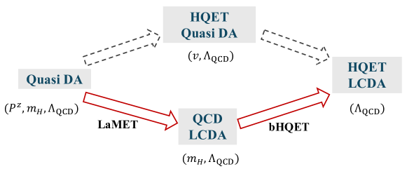
Figure 1: The procedure to calculate the HQET LCDAs. We adopt a two-step matching scheme which makes sequential use of effective field theories. In this approach, one starts with the quasi DAs. After factorizing the hard and collinear degrees of freedom, one can obtain the QCD LCDAs which contains the dynamics far below $P^{z}$. The collinear modes with offshellness $m_{Q}^{2}\sim m_{H}^{2}$ are integrated out and the QCD LCDAs can be matched onto the HQET LCDAs in a boost frame. This procedure is depicted by the red arrows. Another alternative approach that makes use of quasi DAs within HQET is also shown in this figure.

By progressively isolating the higher two scales $P^{z}$ and $m_{H}$ through the utilization of two effective theory factorization formulas via LaMET and boosted HQET (bHQET) sequentially, we can deduce the LCDAs within HQET. A visual representation of this procedure is depicted in Fig. 1. The alternative approach Kawamura:2018gqz ; Wang:2019msf ; Zhao:2020bsx ; Xu:2022krn ; Xu:2022guw ; Hu:2023bba ; Hu:2024ebp that makes use of HQET quasi DA is also incorporated in this figure. This will be beneficial when direct simulation of the HQET heavy quark field on the lattice is straightforward to implement.

It is necessary to stress that using the quasi DAs have the potential to resolve all three obstacles in calculating HQET LCDAs, but the procedure must be properly designed. More explicitly, in the large momentum limit, the quasi-DA involves three distinct scales: the large momentum $P^{z}$, the heavy hadron mass $m_{H}$ which is at leading power equal to the heavy quark mass $m_{Q}$, and the hadronic scale $\Lambda_{\textrm{QCD}}$. We will point out that only for $P^{z}\gg m_{H}\gg\Lambda_{\textrm{QCD}}$, the first two energy scales fall within the perturbative regime and can be integrated out step by step. In the first step, the scale $P^{z}$ can be integrated out, facilitating the matching of the quasi-DA to the LCDA defined in QCD. This is guaranteed by the separation of hard modes with offshellness $\left(P^{z}\right)^{2}$ and collinear modes. This procedure is consistent with the treatment of parton distribution functions (PDFs) and light meson LCDAs in LaMET (for recent developments, please refer to the reviews Ji:2020ect ; Cichy:2018mum ), while a difference is that collinear modes in the present case include both hard-collinear and soft-collinear modes. Once the QCD LCDA is derived, the second step involves integrating out the $m_{H}$ scale and matching the resulting quantity to the LCDA defined in HQET, more explicitly in boosted HQET. Hard-collinear modes with an off-shellness of $m_{Q}^{2}$ are absorbed by the jet function, while the low-energy contributions are accounted for in the HQET LCDAs Ishaq:2019dst ; Beneke:2023nmj . In the subsequent discussion, we will explain in detail who to carry out this two-step matching procedure.

II.1 Step I: Integrating out $P^{z}$

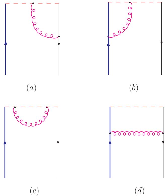
Figure 2: The one-loop Feynman diagrams for $\tilde{M}^{0}(z,0;\gamma^{t}\gamma_{5},m_{H})$ of quasi-DA in Eq. (8). The red dashed line represents the gauge link, while the blue and black line denote the heavy quark and light quark, respectively.

LaMET calculation involves a separation of hard and collinear components Ji:2013dva ; Ji:2014gla , and has a wide range of applications on the lattice, including calculations of quark distribution functions Xiong:2013bka ; Lin:2014zya ; Alexandrou:2015rja ; Chen:2016utp ; Alexandrou:2016jqi ; Alexandrou:2018pbm ; Chen:2018xof ; Lin:2018pvv ; LatticeParton:2018gjr ; Alexandrou:2018eet ; Liu:2018hxv ; Chen:2018fwa ; Izubuchi:2018srq ; Izubuchi:2019lyk ; Shugert:2020tgq ; Chai:2020nxw ; Lin:2020ssv ; Fan:2020nzz ; Gao:2021hxl ; Gao:2021dbh ; Gao:2022iex ; Su:2022fiu ; LatticeParton:2022xsd ; Gao:2022uhg ; Chou:2022drv ; Gao:2023lny ; Gao:2023ktu ; Chen:2024rgi ; Holligan:2024umc ; Holligan:2024wpv , gluon distribution functions Wang:2017qyg ; Wang:2017eel ; Fan:2018dxu ; Wang:2019tgg ; Good:2024iur , generalized parton distributions Chen:2019lcm ; Alexandrou:2019dax ; Lin:2020rxa ; Alexandrou:2020zbe ; Lin:2021brq ; Scapellato:2022mai ; Bhattacharya:2022aob ; Bhattacharya:2023nmv ; Bhattacharya:2023jsc ; Lin:2023gxz ; Holligan:2023jqh ; Ding:2024hkz , distribution amplitudes Zhang:2017bzy ; Chen:2017gck ; Zhang:2020gaj ; Hua:2020gnw ; LatticeParton:2022zqc ; Gao:2022vyh ; Xu:2022guw ; Holligan:2023rex ; Deng:2023csv ; Han:2023xbl ; Han:2023hgy ; Han:2024min ; Han:2024ucv ; Baker:2024zcd ; Cloet:2024vbv ; Han:2024cht ; Deng:2024dkd , transverse-momentum-dependent distributions Ji:2014hxa ; Shanahan:2019zcq ; Shanahan:2020zxr ; Zhang:2020dbb ; Ji:2021znw ; LatticePartonLPC:2022eev ; Liu:2022nnk ; Zhang:2022xuw ; Deng:2022gzi ; Zhu:2022bja ; LatticePartonCollaborationLPC:2022myp ; Rodini:2022wic ; Shu:2023cot ; Chu:2023jia ; delRio:2023pse ; LatticePartonLPC:2023pdv ; LatticeParton:2023xdl ; Alexandrou:2023ucc ; Avkhadiev:2023poz ; Zhao:2023ptv ; Avkhadiev:2024mgd ; Bollweg:2024zet ; Spanoudes:2024kpb , and double parton distribution functions Zhang:2023wea ; Jaarsma:2023woo . Hard modes at the scale $\mu=P^{z}$ are captured in the short-distance coefficient, while the collinear sector, encompassing the low-energy degrees of freedom $(m_{Q}^{2},\Lambda_{\rm QCD}^{2})$, is accounted for within the LCDAs defined with QCD quark fields.

In LaMET, the relevant quasi-DA is defined as

$$\tilde{\phi}(x,P^{z})=\int\frac{dz}{2\pi}e^{-ixP^{z}z}\tilde{M}^{R}(z,P^{z}).$$ (8)

In this context, $\tilde{M}^{R}(z,P^{z})$ represents the renormalized nonlocal matrix element (ME) of a highly boosted heavy meson in coordinate space. Here, we consider the renormalization of the bare ME $\tilde{M}^{B}(z,P^{z};\Gamma)$ which is defined as:

$$\tilde{M}^{B}(z,P^{z};\Gamma)=\frac{\left\langle 0\left|\bar{q}(z)\Gamma W_{c}(z,0)Q(0)\right|H(P^{z})\right\rangle}{\left\langle 0\left|\bar{q}(0)\Gamma Q(0)\right|H(P^{z})\right\rangle},$$ (9)

in the hybrid-ratio scheme Ji:2020brr . The hybrid renormalization involves identifying and subsequently subtracting linear and logarithmic divergences present in bare MEs. This renormalization procedure is carried out in two distinct regions LatticePartonLPC:2021gpi ; Holligan:2023jqh ; Baker:2024zcd :

$$\tilde{M}^{R}\left(z,P^{z}\right)=\begin{cases}\frac{\tilde{M}^{B}\left(z,P^{z};\gamma^{z}\gamma_{5}\right)}{\tilde{M}^{B}\left(z,P^{z}=0;\gamma^{t}\gamma_{5}\right)}&|z|<z_{s}\\ e^{\left(\delta m+m_{0}\right)\left(z-z_{s}\right)}\frac{\tilde{M}^{B}\left(z,P^{z};\gamma^{z}\gamma_{5}\right)}{\tilde{M}^{B}\left(z_{s},P^{z}=0;\gamma^{t}\gamma_{5}\right)}&|z|\geq z_{s}\end{cases}.$$ (10)

Here, $z_{s}$ represents the scale distinguishing the short-distance (perturbative) and long-distance (nonperturbative) regions. $\delta m$ delineates linear divergence within bare matrix elements, stemming from self-energy of Wilson line and influencing the decay properties at large values of $z$. Additionally, $m_{0}$ encapsulates the regularization scheme-specific renormalon ambiguity, arising due to the non-convergence of the perturbation series used to compute $\delta m$ across all orders.

The logarithmic UV divergence within the bare matrix elements, stemming from the perturbative corrections to the quark-Wilson-line vertex, can be eliminated by normalizing certain lattice MEs that exhibit the same divergence. For instance, MEs with the same operator but different external states can be leveraged for this purpose. In our study, we employ the zero-momentum ME $\tilde{M}^{B}\left(z,P^{z}=0;\gamma^{t}\gamma_{5}\right)$ to renormalize the bare MEs. It is important to note that the bare ME in Eq. (9) featuring the Dirac structure $\gamma^{\mu}\gamma_{5}$ is proportional to $P^{\mu}$, thereby making the zero momentum MEs with $\gamma^{z}\gamma_{5}$ equal to zero and unsuitable as renormalization factors. As a substitute, we utilize the zero momentum MEs with $\Gamma=\gamma^{t}\gamma_{5}$, which possess the same UV divergence as those with $\Gamma=\gamma^{z}\gamma_{5}$.

In the regime where the meson momentum $P^{z}$ substantially exceeds the heavy meson mass, the renormalized quasi-DA $\tilde{\phi}(x,P^{z})$ can be matched to the QCD LCDA via the following factorization formula

$$\tilde{\phi}(x,P^{z})= \int_{0}^{1}dy\,C\left(x,y,\frac{\mu}{P^{z}}\right)\phi(y,\mu)$$

$$+\mathcal{O}\left(\frac{m_{H}^{2}}{\left(P^{z}\right)^{2}},\frac{\Lambda_{\mathrm{QCD}}^{2}}{(xP^{z},\bar{x}P^{z})^{2}}\right)$$ (11)

with $\bar{x}=1-x$. $\phi(y,\mu)$ denotes the QCD LCDA in $\overline{\textrm{MS}}$ scheme, which is defined as

$$\phi(y,\mu)=\frac{1}{if_{H}}\int_{-\infty}^{+\infty}\frac{d\tau}{2\pi}\,e^{iyP_{H}\tau n_{+}}$$

$$\qquad\times\left\langle 0\left|\bar{q}(\tau n_{+}){n}\!\!\!/_{+}\gamma_{5}W_{c}(\tau n_{+},0)Q(0)\right|H(P_{H})\right\rangle.$$ (12)

In the above formula $y$ represents the momentum fraction of the light quark in heavy meson $H$. $|H(P_{H})\rangle$ is the heavy meson state with mass $m_{H}$. $f_{H}$ signifies the decay constant in QCD. The $C\left(x,y,\frac{\mu}{P^{z}}\right)$ in Eq.(11) is the matching coefficient

$$C\left(x,y,\frac{\mu}{P^{z}}\right)=~{} \delta(x-y)+C_{B}^{(1)}\left(x,y,\frac{\mu}{P^{z}}\right)$$

$$-C_{CT}^{(1)}\left(x,y\right)+\mathcal{O}(\alpha_{s}^{2}),$$ (13)

where $C_{B}^{(1)}$ is the bare matching kernel, and $C_{CT}^{(1)}$ denotes the counter term in the hybrid-ratio scheme.

It is convenient to perform the calculation in Feynman gauge, and the dimensional regularization ($d\!=\!4\!-\!2\epsilon$) can be utilized to handle both ultraviolet and infrared divergences. The relevant Feynman diagrams at one-loop are shown in Fig. 2. At leading power, we find that the $C_{B}^{(1)}\left(x,y,\frac{\mu}{P^{z}}\right)$ is identical to the matching kernel for the light meson, which has been reported in Ref. Liu:2018tox ,

$$C_{B}^{(1)}\left(x,y,\frac{\mu}{P^{z}}\right)$$

$$= \frac{\alpha_{s}C_{F}}{2\pi}\begin{cases}{\left[H_{1}(x,y)\right]_{+}}&x<0<y\\ {\left[H_{2}\left(x,y,P^{z}/\mu\right)\right]_{+}}&0<x<y\\ {\left[H_{2}\left(1-x,1-y,\frac{P^{z}}{\mu}\right)\right]_{+}}&y<x<1\\ {\left[H_{1}(1-x,1-y)\right]_{+}}&y<1<x\end{cases}\,,$$ (14)

where

$$H_{1}(x,y) =\frac{1+x-y}{y-x}\frac{1-x}{1-y}\ln\frac{y-x}{1-x}$$

$$+\frac{1+y-x}{y-x}\frac{x}{y}\ln\frac{y-x}{-x}\,,$$

$$H_{2}\left(x,y,P^{z}/\mu\right) =\frac{1+y-x}{y-x}\frac{x}{y}\ln\frac{4x(y-x)\left(P^{z}\right)^{2}}{\mu^{2}}$$

$$+\frac{1+x-y}{y-x}\left(\frac{1-x}{1-y}\ln\frac{y-x}{1-x}-\frac{x}{y}\right)\,.$$

In the above formulas, the plus function is defined as

$$\left[h(x,y)\right]_{+}=h(x,y)-\delta(x-y)\int dzh(z,y).$$ (15)

In the hybrid scheme Ji:2020brr , a perturbatively controlled short-distance correction is introduced to eliminate the singularity at $z^{2}\rightarrow 0$ to reconcile perturbation theory and lattice data. The Fourier transform of this correction into momentum space yields the counter-term $\tilde{\phi}_{CT}(x,x_{0},P^{z})$,

$$\tilde{\phi}_{CT}^{(1)}(x,P^{z};x_{0})$$

$$=\int\frac{d\lambda}{2\pi}e^{-i\lambda(x-x_{0})}\frac{\alpha_{s}C_{F}}{2\pi}\frac{3}{2}\ln\left(\frac{\lambda^{2}}{z_{s}^{2}P_{z}^{2}}\right)\theta\left(z_{s}-\left|\frac{\lambda}{P^{z}}\right|\right)$$

$$=-\frac{3\alpha_{s}C_{F}}{4\pi}\frac{2\,\text{Si}[(x-x_{0})z_{s}P^{z}]}{\pi(x-x_{0})}\ ,$$ (16)

where Si denotes the sine integral function. Accordingly, we can determine the counter-term $C_{CT}^{(1)}\left(x,y\right)$:

$$C_{CT}^{(1)}=-\frac{3\alpha_{s}C_{F}}{4\pi}\left[\frac{2\,\text{Si}[(x-y)z_{s}P^{z}]}{\pi(x-y)}\right]_{+}\ ,$$ (17)

where the plus function is introduced to preserve the proper normalization of the distribution. Notably, delta functions are excluded from the above derivation as they vanish within the overall plus function. It should be noted that the counter term is derived in the small spatial separation $z$ and higher power corrections are neglected. Inclusion of power corrections $m_{Q}\times z$ in the future are likely to improve the convergence of perturbation theory, and deserves a detailed analysis.

II.2 Step II: Integrating out $m_{H}$

It is important to note that in HQET, the momentum of a light quark inside a heavy meson at rest is typically soft. Conversely, when the momentum of the light quark is large, with $\omega\sim m_{H}\gg\Lambda_{\mathrm{QCD}}$, the heavy quark will carry a relatively small momentum, referred to as the tail region. In this regime, the HQET LCDA is perturbatively calculable. Thereby it can be handled using QCD perturbation theory, and the one-loop result can be found in Ref. Lee:2005gza

$$\varphi^{+}_{\mathrm{tail}}(\omega,\mu)=\frac{\alpha_{s}C_{F}}{\pi\omega}\bigg{[}\bigg{(}\frac{1}{2}-\ln\frac{\omega}{\mu}\bigg{)}+\frac{4\bar{\Lambda}}{3\omega}\left(2-\ln\frac{\omega}{\mu}\right)\bigg{]},$$ (18)

with $\bar{\Lambda}=m_{H}-m_{Q}$ characterizing the size of power corrections.

When the $\omega$ is small, this is the so-called peak region. In this regime, the QCD LCDA can be matched onto the HQET LCDAs using boosted HQET. Such a matching can be performed by employing heavy quark expansion with $m_{H}\gg\Lambda_{\mathrm{QCD}}$. It leads to a factorization theorem that the LCDA in QCD can be factorized into a multiplication of jet function $\mathcal{J}$ and the HQET LCDA $\varphi^{+}(\omega,\mu)$. This relation was first derived for the inverse moment Pilipp:2007sb and was later generated to LCDAs Ishaq:2019dst ; Beneke:2023nmj and the heavy-light QCD operators Zhao:2019elu .

In this work we will adopt the result reported in Ref. Beneke:2023nmj , in which the matching relation is written as

$$\varphi^{+}_{\mathrm{peak}}(\omega,\mu)=\frac{1}{m_{H}}\frac{f_{H}}{\widetilde{f}_{H}}\frac{1}{\mathcal{J}_{\mathrm{peak}}}\phi(y,\mu;m_{H})$$ (19)

where the perturbative result for $\mathcal{J}_{\text{peak }}$ is given as:

$$\mathcal{J}_{\text{peak }}=1 +\frac{\alpha_{s}C_{F}}{4\pi}\bigg{(}\frac{1}{2}\ln^{2}\frac{\mu^{2}}{m_{H}^{2}}+\frac{1}{2}\ln\frac{\mu^{2}}{m_{H}^{2}}+\frac{\pi^{2}}{12}+2\bigg{)}$$

$$+\mathcal{O}\left(\alpha_{s}^{2}\right),$$ (20)

with $\omega=ym_{H}$, $\bar{y}\equiv 1-y$. $f_{H}$ and $\widetilde{f}_{H}$ are the decay constants of heavy meson in QCD and HQET, respectively. Their relation is given by

$$f_{H}=\tilde{f}_{H}(\mu)\left[1-\frac{\alpha_{s}C_{F}}{4\pi}\left(\frac{3}{2}\ln\frac{\mu^{2}}{m_{Q}^{2}}+2\right)+\mathcal{O}\left(\alpha_{s}^{2}\right)\right].$$ (21)

The factorization formula in Eq. (19) is multiplicative. The scale $\mu$ here satisfies $\Lambda_{\rm QCD}\leq\mu\leq m_{H}$, and the renormalization group equation allows to evolve the HQET LCDAs to a low energy scale.

With the results in Eq. 18 and Eq. (19) for the tail and peak regions repsectively, we can merge them to obtain a full distribution:

$$\varphi^{+}(\omega,\mu)=\left\{\begin{array}[]{lr}\varphi^{+}_{\mathrm{peak}}(\omega,\mu),{}{}{}{}&\omega\sim\Lambda_{\mathrm{QCD}}\\ \\ \varphi^{+}_{\mathrm{tail}}(\omega,\mu).{}{}{}{}&\omega\sim m_{H}\end{array}\right.$$ (25)

The details of merging these two regions will be discussed in Sec.IV.4.

II.3 Theoretical clarifications

In the preceding subsections, we have detailed the two-step matching method that involves the successive application of effective field theories. Beyond the theoretical methodology, there are several noteworthy observations to be highlighted.

• In heavy meson decays, the HQET LCDAs defined in the rest frame with $(v^{\mu}=(1,0,0,0))$ are typically employed. However, in this study, the QCD LCDAs can be matched onto the LCDAs defined in the boosted HQET scenario Fleming:2007qr ; Fleming:2007xt :

  $$\langle 0|\mathcal{O}_{b}^{P}(\omega)|H(p_{H})\rangle= -i\tilde{f}_{H}\varphi^{+}(\omega;\mu),$$ (26)

  The involved bHQET operator is constructed as:

  $$\mathcal{O}_{b}^{P} (\omega)=\frac{1}{m_{H}}\int\frac{dt}{2\pi}e^{-it\omega n_{+}\cdot v}$$

  $$\times\sqrt{\frac{n_{+}\cdot v}{2}}\bar{\xi}_{sc}(tn_{+})\not{n}_{+}\gamma_{5}W_{c}[tn_{+},0]{h}_{n}(0),$$ (27)

  where the soft-collinear field $\xi_{sc}=\frac{\not{n}_{-}\not{n}_{+}}{4}q_{sc}(x)$ describes the light anti-quark in the heavy meson in the boosted frame. The bHQET field $h_{n}$ Dai:2021mxb is given as:

  $$h_{n}(x)\equiv\sqrt{\frac{2}{n_{+}\cdot v}}e^{im_{Q}v\cdot x}\frac{\not{n}_{-}\not{n}_{+}}{4}Q(x),$$ (28)

  which is considered as a hard-collinear field. An analysis based on expansion by region has demonstrated that the matching of QCD LCDAs to HQET LCDAs is the same in these two frames Deng:2024dkd .

• It is important to note that HQET LCDAs are not dependent on heavy quark mass. Therefore, in the methodology, one has the flexibility to choose $m_{Q}$ as the charm quark mass $m_{c}$, the bottom quark mass $m_{b}$, or any other suitable value, with the resulting HQET LCDAs remaining unchanged. Discrepancies observed in the obtained results can indicate the presence of power corrections. In the following simulation we will choose $m_{Q}=m_{c}$.

• Given that HQET LCDAs are not influenced by the heavy quark mass, the mass dependence of QCD LCDAs can be deduced, leading to the derivation of an evolution equation for this mass dependence. This process aligns with the concept of a renormalization group equation, which can enhance the power expansion in relation to $(\Lambda_{\text{QCD}}/m_{Q})$. Furthermore, employing QCD LCDAs to derive HQET LCDAs aligns with the principle of LaMET, which illustrates that lightcone observables, traditionally defined in the infinite momentum limit, can be accessed using a finite yet large $P^{z}$. Likewise, exploring observables related to heavy quarks defined in HQET is achievable through utilizing quantities that involve a large yet finite heavy quark mass.

• In heavy quark limit $(m_{Q}\to\infty)$, the interaction becomes uncorrelated with heavy quark spin, establishing the presence of heavy quark spin symmetry. As a result, the identical HQET LCDAs can be defined for a heavy vector meson:

  $$\langle 0|O_{v}^{||}(tn_{+})|H^{*}(p_{H},\eta)\rangle= \tilde{f}_{H}m_{H}n_{+}\cdot\eta$$

  $$\times\int_{0}^{\infty}d\omega e^{i\omega tn_{+}\cdot v} \varphi^{+}(\omega;\mu),$$

  $$\langle 0|O_{v}^{\perp\mu}(tn_{+})|H^{*}(p_{H},\eta)\rangle= \tilde{f}_{H}m_{H}n_{+}\cdot v\eta_{\perp}^{\mu}$$

  $$\times\int_{0}^{\infty}d\omega e^{i\omega tn_{+}\cdot v} \varphi^{+}(\omega;\mu),$$ (29)

  where $\eta$ is the polarization vector. The involved operators are given as:

  $$O_{v}^{||}(tn_{+})= \,\bar{q}_{s}(tn_{+})\not{n}_{+}W_{c}[tn_{+},0]{h}_{v}(0),$$

  $$O_{v}^{\perp\mu}(tn_{+})= \,\bar{q}_{s}(tn_{+})\not{n}_{+}\gamma^{\mu}_{\perp}W_{c}[tn_{+},0]{h}_{v}(0).$$ (30)

  Building upon this symmetry, a recent study demonstrates that quasi distribution amplitudes for a vector meson can also be employed to extract the same HQET LCDAs Deng:2024dkd . Discrepancies in these extractions arise from power corrections attributed to the breaking of heavy quark spin symmetry.

• The factorization scheme in the present work operates at the leading power level. In the first step the factorization of hard and collinear modes, the power expansion is conducted in terms of $m_{H}^{2}/\left(P^{z}\right)^{2}$, and $\Lambda_{\mathrm{QCD}}^{2}/(xP^{z})^{2},\Lambda_{\mathrm{QCD}}^{2}/((1-x)P^{z})^{2}$. Some power corrections, target mass corrections with $m_{H}^{2}/\left(P^{z}\right)^{2}$, have been estimated, and $\Lambda_{\mathrm{QCD}}^{2}/(xP^{z})^{2}$ corrections are estimated using a renormalon model  Han:2024cht . The findings suggest that these corrections typically fall below $20\%$, but it is important to note that other power corrections, particularly those in the subsequent step involving terms of $\Lambda_{\mathrm{QCD}}/m_{Q}$, have not yet been explored.

• The two-step matching method derives the HQET LCDAs only in the peak region. However, in order to integrate the perturbative result in the endpoint region, a strategy for their combination must be devised. In bringing together these outcomes, it is crucial to identify a region where both predictions are anticipated to be accurate. A suitable selection for this integration is around $\omega\sim 1$GeV.

• In LaMET, the prediction for QCD LCDAs is uncertain in the region where $y\sim\Lambda_{\mathrm{QCD}}/P^{z}$. This translates to $\omega=ym_{H}\sim\Lambda_{\mathrm{QCD}}/P^{z}\times m_{H}$. For typical values of $P^{z}\sim(3-4)$ GeV and $m_{H}\sim(1.5-2)$ GeV, this corresponds to $y\sim 0.1$ and $\omega\sim 0.2$ GeV, which falls below the peak region of HQET LCDAs. To match such high momenta, lattice ensembles with a lattice spacing of $a\lesssim 0.05$ fm are required and will be used in our lattice simulation.

III Lattice simulation

III.1 Lattice setup

The numerical simulation in this work is performed on the gauge configuration generated by China Lattice QCD (CLQCD) collaboration with $N_{f}=2+1$ flavor stout smeared clover fermions and Symanzik gauge action Hu:2023jet . One step of Stout link smearing is applied to the gauge field used by the clover action to improve the stability of the pion mass for given bare quark mass. In this work, we adopt a single ensemble (named “H48P32” in Ref.Hu:2023jet ) at the finest lattice spacing $a=0.05187$fm and volume $L^{3}\times T=48^{3}\times 144$ with sea quark masses corresponding to $m_{\pi}=317.2$MeV and $m_{K}=536.1$MeV. Furthermore, we determine the charm quark mass by requiring the corresponding $J/\psi$ mass to have its physical value $m_{J/\psi}=3.96900(6)$GeV within $0.3\%$ accuracy, hence the heavy $D$ meson mass on this ensemble is calibrated as $m_{D}=1.917(5)$GeV. These configurations have been successfully applied in studies involving hadron spectrum Liu:2022gxf ; Xing:2022ijm ; Yan:2024yuq , decay and mixing of charmed hadron Zhang:2021oja ; Liu:2023feb ; Liu:2023pwr ; Meng:2024nyo ; Du:2024wtr ; Chen:2024rgi and other interesting phenomena Zhao:2022ooq ; Meng:2023nxf .

From a total of 549 gauge configurations, we use 8784 measurements of the bare MEs of heavy $D$ meson with boosted momentum $P^{z}=\{0,~{}6,~{}7,~{}8\}\times 2\pi/(La)\simeq\{0,~{}2.99,~{}3.49,~{}3.98\}$GeV respectively. To improve the signals, we adopt the plane source on the Coulomb gauge fixed configurations, which involves summing over all spatial sites along the $x$ and $y$ directions for each time slice. The advantage of using this particular source lies in its ability to produce good correlation signals through the summation of spatial wave functions across all sites in the $x$ and $y$ directions. Simultaneously, the fixed positional coordinates along the $z$ axis guarantee the ability to obtain any momentum values following a Fourier transformation.

We use the grid-source-to-point-sink propagators

$$G_{f}(x^{3},t,t_{0})\equiv\sum_{\vec{y}}\sum_{\vec{x}}D^{-1}_{f}(t,\vec{y};t_{0},\vec{x})e^{i\vec{p}\cdot(\vec{x}-\vec{y})},$$ (31)

where $D^{-1}_{f}(t,\vec{y};t_{0},\vec{x})$ denotes the $f$-flavored quark propagator from $(t_{0},\vec{x})$ to $(t,\vec{y})$. The summation of $\vec{x}=(x^{1},x^{2})$ corresponds to the summing over all spatial sites along $x$ and $y$ directions of the grid source, and the residual $x^{3}$ will contribute to the momentum of the hadronic external state in the nonlocal two point function (2pt),

$$C_{2}(z,P^{z},t;\Gamma)= \sum_{x^{3}}e^{iP^{z}x^{3}}\left\langle G_{q}(x^{3}+z,t,0)\Gamma\right.$$

$$\times\left.W_{c}(x^{3}+z,x^{3})\gamma_{5}G_{Q}^{\dagger}(x^{3},t,0)\right\rangle,$$ (32)

where $z$ denotes the spatial separation between the light and heavy quarks within the nonlocal quark operator, and $W_{c}(x^{3}+z,x^{3})$ is the spatial Wilson line along the $z$ direction that ensures gauge invariance. The matrix $\Gamma=\gamma^{t}\gamma_{5}$ or $\gamma^{z}\gamma_{5}$ serves as the Dirac matrix that can be projected onto $\gamma^{+}\gamma_{5}$ in the large momentum limit, which is related to the leading twist LCDAs. When the lattice operators incorporate $\gamma^{t}\gamma_{5}$, they induce chiral symmetry breaking at finite lattice spacings and intertwine with other operators Constantinou:2017sej ; Chen:2017mzz ; Liu:2018tox . Consequently, we opt for $\Gamma=\gamma^{z}\gamma_{5}$ to establish correlations corresponding to large momentum MEs. For the zero momentum ME, we choose $\Gamma=\gamma^{t}\gamma_{5}$, as this ME is directly proportional to $P^{\mu}$ in the local limit and becomes null when $\Gamma=\gamma^{z}\gamma_{5}$.

III.2 Extraction of bare matrix elements

By incorporating single-particle intermediate state, the nonlocal two point correlation function in Eq. 32 can be parameterized as:

$$C_{2}(z,P^{z},t;\Gamma) =\sum_{n}\frac{1}{2E_{n}}e^{-E_{n}t}\langle n(P^{z})|\bar{Q}(0)\gamma_{5}q(0)|0\rangle$$

$$\times\left\langle 0|\bar{q}(z)\Gamma W_{c}(z,0)Q(0)|n(P^{z})\right\rangle.$$ (33)

The local ME is related to the decay constant of heavy meson in QCD:

$$\langle n(P^{\mu})|\bar{Q}\gamma_{5}q|0\rangle=if_{H^{(*)}}P^{\mu}.$$ (34)

After taking a ratio of nonlocal and local 2pt, we can obtain the $R(z,P^{z},t;\Gamma)$

$$R(z,P^{z},t;\Gamma)\equiv\frac{C_{2}(z,P^{z},t{;\Gamma})}{C_{2}(0,P^{z},t;\Gamma)},$$ (35)

which can be expanded as

$$R(z,P^{z},t;\Gamma) =e^{-E_{0}t}\left\langle 0|\bar{q}(z)\Gamma W_{c}(z,0)Q(0)|H(P^{z})\right\rangle$$

$$+e^{-E_{1}t}\left\langle 0|\bar{q}(z)\Gamma W_{c}(z,0)Q(0)|H_{1}^{*}(P^{z})\right\rangle$$

$$+\cdots,$$ (36)

in which $H_{n}^{*}$ denotes the excited states of the pseudoscalar heavy meson $H$ with energy level $E_{n}$. One can extract $E_{n}$ as well as the ground-state ME $\tilde{M}^{B}(z,P^{z};\Gamma)$ from a multi-state fit of $R(z,P^{z},t;\Gamma)$, with the parametrization

$$R(z,P^{z},t;\Gamma) =\tilde{M}^{B}(z,P^{z};\Gamma)e^{-E_{0}t}\left[\sum_{n=0}^{N_{\mathrm{stat}}-1}A_{n}e^{-(E_{n}-E_{0})t}\right].$$ (37)

Here $A_{0}=1$, and $A_{n}$ denotes the contribution of ME at $n$-th excited state and can be determined from fitting the $t$-dependence of $R(z,P^{z},t;\Gamma)$.

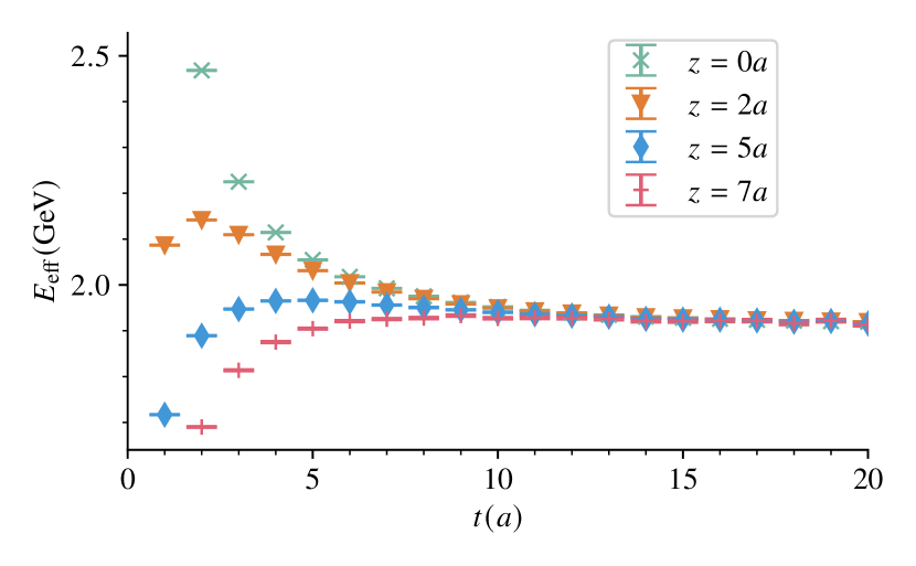
Figure 3: Effective energies of nonlocal 2pt $C_{2}(z,P^{z}=0,t;\gamma^{t}\gamma_{5})$ at different $z$, which is defined as $E_{\mathrm{eff}}=\ln C_{2}(z,P^{z},t;\Gamma)/C_{2}(z,P^{z},t+1;\Gamma)$ and will converge to $E_{0}$ at sufficiently large $t$. All the data tend to converge on the same plateau at large $t$, suggesting that they share the same ground-state energy.

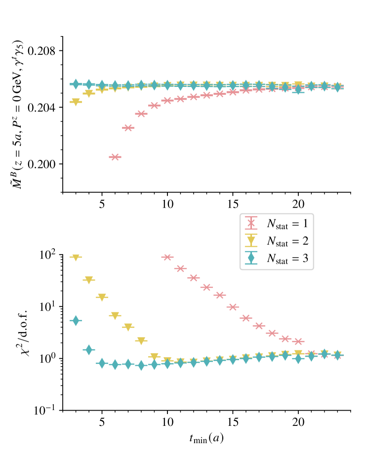
Figure 4: Upper panel: The fitting results of the ground-state ME $\tilde{M}^{B}(z,P^{z}=0;\gamma^{t}\gamma_{5})$ from one-state, two-state, and three-state fit with a fit range $t\in[t_{\mathrm{min}},31a]$. Lower panel: The $\chi^{2}/$d.o.f. values of the fits.

We will conduct the fitting using one-state ($N_{\mathrm{stat}}=1$), two-state ($N_{\mathrm{stat}}=2$), and three-state ($N_{\mathrm{stat}}=3$) ansatz. First we exam the behavior of effective energies of the nonlocal 2pt $C_{2}(z,P^{z}=0,t;\gamma^{t}\gamma_{5})$ at different $z$. As shown in Fig. 3, it is observed that all curves of $E_{\mathrm{eff}}(z)$ with the same external momentum $P$ exhibit a common plateau at large $t$. To ensure the success of the one-state fits, it is necessary to utilize the data from sufficiently large $t$ values (e.g., $t\geq t_{\mathrm{min}}\simeq 13a$ for $z=2a$ case, or $t_{\mathrm{min}}\simeq 6a$ for $z=5a$ case in Fig. 3) to capture the plateau behavior. However, achieving this scenario is often challenging due to the signal-to-noise ratio in the nonlocal correlation functions, which tends to increase more rapidly for large momenta or spatial separations. This suggests that for the highly boosted nonlocal 2-point functions under consideration, the potential plateau behavior at large $t$ might be obscured by rapidly growing errors. As higher excited states possess larger energies, their contributions diminish quickly with the increase of $t$. Consequently, we can introduce the two-state, three-state (or even higher states) fits step by step by gradually reducing the value of $t_{\mathrm{min}}$ for each fit.

In the upper panel of Fig. 4, we compare the results of the ground-state ME $\tilde{M}^{B}(z,P^{z}=0;\gamma^{t}\gamma_{5})$ obtained from one-state, two-state, and three-state fits with a fit range of $t\in[t_{\mathrm{min}},31a]$. It is evident that the results from all three fitting strategies stabilize and converge with each other when $t_{\mathrm{min}}>20a$. The lower panel displays the $\chi^{2}$/d.o.f. values, further confirming that in this region: the $\chi^{2}$/d.o.f. values from the three fitting strategies are all slightly less than 1, indicating the reliability of the fits. When $t_{\mathrm{min}}$ is decreased from $20a$ to $10a$, deviations in the results from the one-state fits are observed, accompanied by an exponential increase in $\chi^{2}$ /d.o.f.. This behavior suggests that the contribution from the first excited state becomes significant, rendering a single-state parametrization inadequate to describe the data. Continuing to decrease $t_{\mathrm{min}}$, the effectiveness of the two-state fit diminishes as well, indicating the need to include more excited states to capture the more pronounced changes in the data.

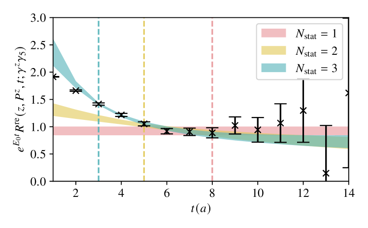
(a) $P^{z}=2.99$GeV, $z=9a$

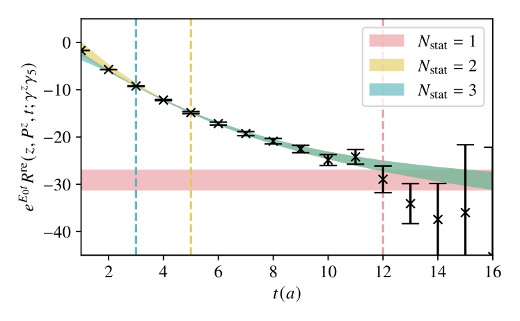
(b) $P^{z}=3.49$GeV, $z=5a$

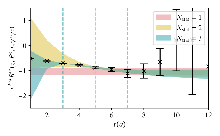
(c) $P^{z}=3.98$GeV, $z=10a$

Figure 5: Comparison of the original lattice data $e^{E_{0}t}R^{\mathrm{re}}(z,P^{z},t;\gamma^{z}\gamma_{5})$ with large $P^{z}$ and $z$, along with the fit results of $\tilde{M}^{B}(z,P^{z};\gamma^{z}\gamma_{5})$ obtained using three fitting strategies. We choose the combinations for $(P^{z},z)=(2.99\mathrm{GeV},9a),(3.49\mathrm{GeV},5a)$ and $(3.98\mathrm{GeV},10a)$ as examples to demonstrate the consistency of the results obtained from three fitting strategies. The solid lines of varying colors represent the different $t_{\mathrm{min}}$ values utilized in each fit.

In practice, it is important to strike a balance between the number of excited states included and the fit range utilized in the fitting process. A conservative approach involves first performing the ground state fit over a sufficiently large range of $t$, after excluding excited-state contaminations. However, this may not always be feasible, especially in situations where the signal-to-noise ratio increases rapidly. In such cases, it becomes necessary to judiciously reduce the value of $t_{\mathrm{min}}$ and incorporate the contributions from higher states to accurately describe the data.

In Fig. 5, we present a comparison of the original lattice data with large momentum $P^{z}$ and spatial separation $z$, along with the fit results obtained using three different strategies. The fits are carried out based on the parametrization form in Eq. (37). To ensure that the ground state MEs eventually converge to a plateau at large $t$, we display the vertical axis as $e^{E_{0}t}R(z,P^{z},t)$. The various colored vertical dashed lines in the plots indicate the values of $t_{\mathrm{min}}$ utilized in the different fit strategies. It is evident that the signal-to-noise ratio of the original data experiences rapid growth and becomes unstable at large $t$. In such scenarios, there may be limited data available to effectively constrain the parameters when employing a one-state fit. By incorporating more excited states, we can utilize data from smaller $t$ values to better constrain the fit parameters. It is noticeable that the $t_{\mathrm{min}}$ values used for two-state and three-state fits gradually decrease, while the final fitting results from all three strategies remain consistent.

Table 1: List of the fitting strategies and $t$ range utilized to extract all the large momentum MEs $\tilde{M}^{B}(z,P^{z};\gamma^{z}\gamma_{5})$.

$z$	$P^{z}=2.99$GeV	$P^{z}=3.49$GeV	$P^{z}=3.98$ GeV
0	1-state, [11,16]	2-state, [6,15]	2-state, [6,13]
1	1-state, [11,16]	2-state, [6,15]	2-state, [6,13]
2	1-state, [11,16]	2-state, [6,15]	2-state, [6,13]
3	1-state, [11,16]	2-state, [5,15]	2-state, [5,13]
4	1-state, [11,16]	2-state, [5,14]	2-state, [5,13]
5	1-state, [11,14]	2-state, [5,13]	2-state, [5,13]
6	1-state, [11,14]	2-state, [5,13]	2-state, [5,13]
7	1-state, [11,14]	2-state, [5,12]	2-state, [5,12]
8	1-state, [11,14]	2-state, [5,10]	1-state, [8,12]
9	1-state, [11,14]	2-state, [5,9]	1-state, [8,11]
10	1-state, [11,14]	2-state, [5,9]	1-state, [8,11]
11	1-state, [11,14]	1-state, [8,13]	1-state, [8,11]
12	1-state, [10,14]	1-state, [8,11]	1-state, [8,11]
13	1-state, [10,14]	1-state, [8,11]
14	1-state, [10,14]	1-state, [7,11]
15	1-state, [10,14]
16	1-state, [10,14]

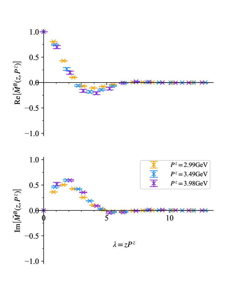
Figure 6: Bare MEs of quasi DA $\tilde{M}^{B}(z,P^{z};\gamma^{z}\gamma_{5})$ with boosted momenta $P^{z}=\{2.99,~{}3.49,~{}3.98\}$GeV. Both real and imaginary parts are shown as function of $\lambda=zP^{z}$.

In summary, the fitting strategies and $t$ ranges utilized to extract all $\tilde{M}^{B}(z,P^{z};\gamma^{z}\gamma_{5})$ are summarized in Tab. 1. For each fit, we initially assess the consistency of results obtained from different strategies, and subsequently determine the final fitting approach based on an evaluation of the fit quality. During the selection process, preference is given to the more conservative one-state fit. Only under conditions where the $\chi^{2}$ /d.o.f. of the fit exceeds 1, or when there are fewer than 4 effective data points available for fitting (to prevent overfitting), we resort to the two-state fit. The three-state fits are solely employed to validate the reliability of the results obtained from the initial two strategies and will not be used to derive the final outcomes.

From the aforementioned deliberations, we ultimately derive the results for the bare MEs of quasi DA $\tilde{M}^{B}(z,P^{z};\gamma^{z}\gamma_{5})$ with the boosted momenta $P^{z}=\{2.99,~{}3.49,~{}3.98\}$GeV, illustrated in Fig. 6. Both real and imaginary parts are shown as functions of $\lambda=zP^{z}$ in this figure. From this figure, one can see that these results exhibit consistency across various momentum values.

III.3 Dispersion relation

Before delving into further discussions, it is essential to verify the dispersion relation for the heavy meson. The effective energies with different momenta can be deduced from $R(z=0,P^{z},t)$ with $\Gamma=\gamma^{t}\gamma_{5}$. By applying the fitting methodologies outlined in the preceding subsection, we can acquire the outcomes for the ground state (from both two- and three-state fits) and the first excited state (from the three-state fit), as depicted in Fig. 7.

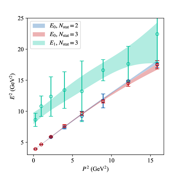
Figure 7: The dispersion relation of heavy $D$ meson with boosted momenta up to 3.98GeV. Two-state and three-state fits strategies are used to extract the ground-state (and first excited state from the latter one) energies. All the fit bands are consistent with the data points well.

For illustration, we adopt the following parametrization form to investigate the dispersion relation

$$E(P^{z})=\sqrt{m^{2}+c_{0}\left(P^{z}\right)^{2}+c_{1}\left(P^{z}\right)^{4}a^{2}},$$ (38)

where a quadratic term of the lattice spacing $a$ is introduced to account for discretization errors. The fit results are shown as the bands in Fig.7. For the ground state energy $E_{0}$ obtained from the two-state fit, we find that $m=1.917(5)$GeV and $c_{0}=0.977(23)$, $c_{1}=-0.072(25)$; for the ground state energy $E_{0}$ from three-state fit, we have $m=1.915(6)$GeV and $c_{0}=1.007(30)$, $c_{1}=-0.124(45)$. We have also conducted a fit for the dispersion relation of the first excited state, resulting in $E_{1}=2.98(16)$GeV, $c_{0}=1.00(43)$, $c_{1}=-0.21(49)$. These findings indicate that the results are fairly consistent with the relativistic dispersion relation up to possible $P_{z}^{2}a^{2}$ discretization error. Therefore, for a moving heavy meson with momenta up to 4 GeV, the discretization effects on the ensemble we utilized remain controllable on this lattice ensemble.

IV Numerical results for LCDAs

IV.1 Renormalization in the hybrid scheme

Based on the renormalization formula in Eq.(10), we will proceed with the renormalization of the bare MEs $\tilde{M}^{B}(z,P^{z};\Gamma)$ in the hybrid-ratio scheme. As discussed in Sec.II.1, an important concept in hybrid renormalization involves identifying and addressing the linear and logarithmic divergences in the bare MEs, followed by subtracting them in distinct regions.

In the long-distance region where $|z|\geq z_{s}$, the renormalization factors will encompass additional non-perturbative effects arising from the conversion of lattice results obtained at a finite spacing $a$ to a continuum scheme. Their explicit origins are given as follows.

• $\delta m$ characterizes the linear divergence, which comes from the self-energy of the Wilson line in the bare ME, and governs the decay behavior at large-$z$. It can be extracted from fitting the long-range correlations of the zero momentum ME.

• $m_{0}$ characterizes the regularization scheme dependent renormalon ambiguity, which arises from the fact that the perturbation series used to calculate $\delta m$ is not convergent to all orders. It can be determined from matching the lattice data of zero momentum MEs at small-$z$ range to the perturbative one.

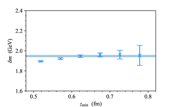
Figure 8: Results of $\delta m$ by fitting the zero momentum MEs in the fit range $z\in[z_{\mathrm{min}},z_{\mathrm{min}}+4a]$. It can be observed that the results of $\delta m$ converge after $z_{\mathrm{min}}>12a\simeq 0.62$fm, then we obtain its value from a constant fit, as shown by the horizontal band.

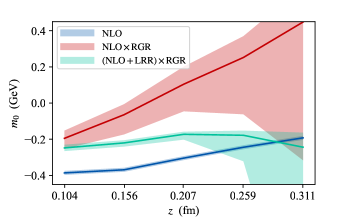
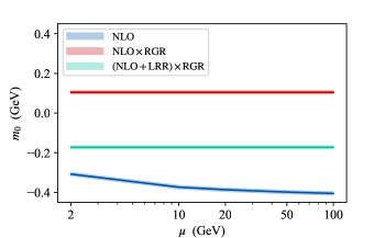
Figure 9: Upper panel: Results of $m_{0}$ from Eq.(42) with the perturbative Wilson coefficient schemes: “NLO”, “NLO$\times$RGR” and “(NLO+LRR)$\times$RGR”. The fitting is carried out in the range $[z-a,z+a]$ for each $z$. Both statistical and systematic errors are included, where the latter one comes from the scale variation of $\mu_{0}$. Lower panel: The scale dependence of $m_{0}$ from different schemes. Only statistical error is included in each bands.

The $\delta m$ can be determined by fitting the MEs according to the exponential decay behavior $Ae^{-\delta mz}$ in the large-$z$ range Ji:2020brr . In principle, the parameter $\delta m$ should depend on the lattice spacing $a$ and the regularization scheme. However, with only one lattice spacing available at this stage, $\delta m$ is treated as a constant Holligan:2023jqh . Since $\delta m$ is independent of the momentum of the external state, it can be extracted by fitting the ME at zero momentum. In practice, we select the fitting range $z\in[z_{\mathrm{min}},z_{\mathrm{min}}+4a]$ with $z_{\mathrm{min}}$ varying from $10a$ to $15a$ to assess the stability of the fits. The specific results obtained from different $z$-ranges are depicted as data points in Fig. 8. It is observed that the values of $\delta m$ obtained from different intervals in the large-$z$ region are consistently around 1.9 GeV, indicating the universality of the extracted $\delta m$. By performing a constant fit of the $\delta m$ values from different $z_{\mathrm{min}}$ values, the exact value of $\delta m$ is determined to be $\delta m=1.948(11)$ GeV, as shown by the band in Fig.8.

After removing the linear divergence, there still remains an $a$-independent term $m_{0}$ collecting the renormalon ambiguity and other effects Ji:2020brr . At small-$z$ region, where the perturbation theory works well, one can extract $m_{0}$ by matching the renormalized zero momentum ME to the continuum perturbative $\overline{\mathrm{MS}}$ result of the Wilson coefficient $C_{0}(z,\mu)$ Baker:2024zcd

$$\tilde{M}^{B}(z,0;a) e^{\left(\delta m(a)+m_{0}\right)z}=$$

$$\qquad C_{0}\left(z,\mu_{0}\right)e^{-\mathcal{I}\left(\mu_{0}\right)}e^{\mathcal{I}^{\mathrm{lat}}\left(a^{-1}\right)}.$$ (39)

Here $\mathcal{I}(\mu)=\int_{\alpha_{s}(\mu_{0})}^{\alpha_{s}(\mu)}d\alpha\frac{\gamma(\alpha)}{\beta(\alpha)}$ denotes the renormalization group resummation (RGR) improvement that cancels the renormalization scheme dependence of the results between lattice scale $\mu_{0}=2e^{-\gamma_{E}}z^{-1}$ and perturbative $\overline{\mathrm{MS}}$ scale $\mu$. The result of Wilson coefficient up to the next-to-leading order (NLO) in $\alpha_{s}$ reads

$$C_{0}^{\mathrm{NLO}}(z,\mu)=1+\frac{\alpha_{s}C_{F}}{2\pi}\left[\frac{3}{2}\log\left(\frac{1}{4}e^{2\gamma_{E}}z^{2}\mu^{2}\right)+A\right],$$ (40)

where the coefficient $A=5/2$ for $\Gamma=\gamma^{t}/\gamma^{t}\gamma_{5}$ cases LatticePartonLPC:2021gpi ; LatticeParton:2022zqc ; Yao:2022vtp and $A=7/2$ for $\Gamma=\gamma^{z}/\gamma^{z}\gamma_{5}$ cases Holligan:2023rex ; Yao:2022vtp . Since the fixed-order result contains large constants due to the renormalon divergence, which influences the perturbative convergence, we apply the leading renormalon resummation (LRR) method Zhang:2023bxs to account for this effect. We then modify the Wilson coefficient as suggested in Zhang:2023bxs ; Holligan:2023jqh :

$$C_{0}^{\mathrm{NLO+LRR}}(z,\mu)=C_{0}^{\mathrm{NLO}}(z,\mu)$$

$$\qquad+z\mu\left(C_{\mathrm{PV}}(z,\mu)-\sum_{i=0}^{k-1}\alpha_{s}^{i+1}(\mu)r_{i}\right),$$ (41)

where $r_{i}$ denote the coefficients of the renormalon series in $\alpha_{s}$ and $C_{\mathrm{PV}}(z,\mu)$ denotes the leading renormalon contribution for $C_{0}$ after a Borel transformation. The explicit forms of $r_{i}$ and $C_{\mathrm{PV}}$ can be found in Eqs.(12) and (13) of Ref. Zhang:2023bxs .

For a single lattice spacing $a$, Eq.(39) can be written as

$$(m_{0}+\delta m)z-I_{0}=\ln\left[\frac{C_{0}^{\mathrm{NLO(+LRR)(\times RGR)}}\left(z,\mu\right)}{\tilde{M}^{B}(z,0)}\right],$$ (42)

where $I_{0}=\mathcal{I}^{\mathrm{lat}}\left(a^{-1}\right)$ is a constant, and the RGR improvement provides the scale conversion from lattice scale $z^{-1}$ to the renormalization scale $\mu$ in $\overline{\mathrm{MS}}$ scheme.

In the region $0\ll z<z_{s}$ , where perturbation theory is effective and discretization effects are not too large, we fit $m_{0}$ and $I_{0}$ based on Eq.(42) over multiple ranges of $z$ up to a maximum of $z\simeq 0.3$ fm. The fitting is carried out in the range $[z-a,z+a]$ for each $z$, using four different perturbative Wilson coefficient schemes: “NLO” representing the fixed-order (NLO) $C_{0}$ at scale $\mu=m_{D}$, “NLO$\times$RGR” including the RGR improvement of $C_{0}$, and “$\mathrm{(NLO+LRR)}\times\mathrm{RGR}$” combining both LRR and RGR improvements. The fit results with these different schemes are presented in the upper panel of Fig.9, showing both statistical and systematic errors. The systematic errors are assessed by varying the lattice scale $\mu_{0}$ within a range from 0.8 to 1.2, accounting for the scaling uncertainties inherent in the lattice results.

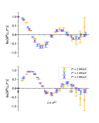
Figure 10: The renormalized MEs of quasi DA $\tilde{M}^{R}(z,P^{z})$ obtained from $z_{s}=6a$ with boosted momenta $P^{z}=\{2.99,~{}3.49,~{}3.98\}$GeV. Both real and imaginary parts are shown as function of $\lambda=zP^{z}$.

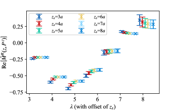
Figure 11: The $z_{s}$ dependence of $\tilde{M}^{R}(z,P^{z})$ at fixed $P^{z}=2.99$GeV. We compare the results from $z_{s}\in[3,8]a$ and find that at $z_{s}\geq 6a\simeq 0.31$fm, the results of $\tilde{M}^{R}(z,P^{z})$ becomes consistent with each other.

Notice that the errors of “NLO$\times$RGR” are significant larger than the ones of “$\mathrm{(NLO+LRR)}\times\mathrm{RGR}$”, which mainly come from the systematic errors by varying the lattice scale $\mu_{0}$. This reflects the systematic errors of fixed-order perturbation theory. Without performing the LRR improvement, the contributions from renormalons would be more significant, and contribute to a larger error after combining the variation of $\mu_{0}$. When including the leading renormalon, the result labeled as “(NLO+LRR)$\times$RGR” displays a clear plateau around $z\simeq 0.2$ fm in the values of $m_{0}$, that indicates the LRR improvement can significantly reduce the dependence on $z$. We choose the result $m_{0}=(-0.173^{+0.014}_{-0.029})$GeV at $z=0.207$ fm, which exhibits a clear plateau. Consequently, the selection of $z_{s}$ should be $z_{s}\gtrsim 0.3$ fm.

We also investigate the scale dependence of $m_{0}$ to assess the impact of unaccounted higher-order terms in $C_{0}$. We compare the extracted results of $m_{0}$ from fixed-order $C_{0}^{\mathrm{NLO}}(z,\mu)$, as well as from the RGR improvement $C_{0}^{\mathrm{NLO\times RGR}}(z,\mu)$ and $C_{0}^{\mathrm{(NLO+LRR)}\times\mathrm{RGR}}(z,\mu)$. The results are shown in the lower panel of Fig.9. One can see from the comparison that the RGR method significantly enhances the stability of $m_{0}$ after scale variation.

After removing the linear divergence and renormalon ambiguity, the renormalized MEs as a function of $\lambda=zP^{z}$ are depicted in Fig. 10. The MEs at different momenta exhibit reasonable consistency, indicating the saturation of equal-time correlations at large $P^{z}$. In showing the results, we have chosen $z_{s}=6a$, where $z_{s}$ represents the boundary between perturbative and nonperturbative regions, with $\mathcal{O}(z_{s}^{-1})$ typically chosen to be around hundreds of MeV to a few GeV. In Fig.11, we show the $z_{s}$ dependence of the real part of the renormalized ME at $P^{z}=2.99$GeV. It is observed that for $z_{s}\geq 6a\simeq 0.31$ fm, the renormalized MEs converge and show consistency, in line with the earlier observation. Additionally, the differences between $z_{s}=(6,7,8)a$ are nearly imperceptible. Consequently, we choose $z_{s}=6a$ for the rest of this study.

IV.2 Extrapolating the long-range correlations

Due to the finite volume of gauge ensembles and the exponential increase in signal-to-noise ratio with spatial separation, the lattice results of nonlocal equal-time correlations tend to exhibit large uncertainties in the large-$\lambda$ region. To reconstruct the complete distributions, we make the following assumption, drawing inspiration from the asymptotic behavior in the long-tail region $e^{-\delta mz}c_{1}/|\lambda|^{d_{1}}$ Ji:2020brr ; Gao:2021dbh . In this scenario, the exponential decay behavior is governed by the linear divergence factor $\delta m$, similar in the zero-momentum MEs. Considering the definition in Eq.(10), the decay factor in the renormalized MEs is $e^{-|m_{0}|(z-z_{s})}$ (please note $m_{0}$ is negative, and thus $m_{0}=-|m_{0}|$). This behavior can be converted to correlation length using the relation $\lambda_{0}\simeq P^{z}/|m_{0}|$. When the momentum $P^{z}$ approaches infinity, the exponential decay behavior vanishes, leaving only the leading-twist contribution that decays algebraically at large $\lambda$.

Therefore, we extrapolate the renormalized MEs by using the following form: Ji:2020brr

$$\tilde{M}^{R}(\lambda)=\left[\frac{c_{1}}{(-i\lambda_{1})^{d_{1}}}+e^{i\lambda}\frac{c_{2}}{(i\lambda_{2})^{d_{2}}}\right]e^{-\lambda/\lambda_{0}},$$ (43)

where the parameterization inside the square brackets account for the algebraic behavior and is motivated by the Regge behavior Regge:1959mz of the light-cone distributions at endpoint regions.

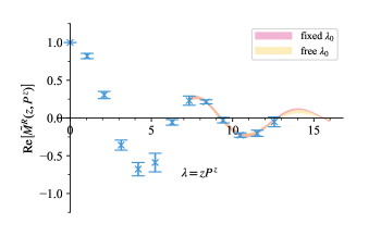
Figure 12: The comparison of extrapolated results from fix the parameter $\lambda_{0}$ from the long-tail behavior of zero-momentum MEs, or treat it as a free parameter. We take the real part of $\tilde{M}^{R}(\lambda)$ at $P^{z}=3.98$GeV as example, and one can see that the extrapolated result from “fixed $\lambda_{0}$” is consistent with “free $\lambda_{0}$”, while giving stricter restrictions of the errors.

As outlined earlier, the $m_{0}$ (and thereby $\lambda_{0}$) can be obtained by fitting the zero-momentum MEs, where the uncertainties are significantly smaller compared to those wither a higher momenta. This can provide a more stringent constraint on the fitting procedure. To illustrate this point, we conducted a comparison between two fitting strategies: one involving a “fixed $\lambda_{0}$” determined by the result of $m_{0}$, and the other using a “free $\lambda_{0}$” parameter in the fit Gao:2021dbh . The comparison of these two strategies is presented in Fig. 12. It is evident from the figure that the extrapolated bands obtained from both strategies are in agreement, while the errors associated with the “fixed $\lambda_{0}$” approach are considerably smaller. To prevent underestimation of errors, we opt to employ the “free $\lambda_{0}$” strategy in our subsequent analysis.

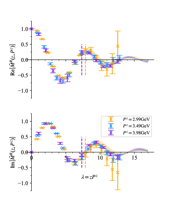
Figure 13: Comparison of the original (data points) and extrapolated results (colored bands) at $P^{z}=\{2.99,~{}3.49,~{}3.98\}$GeV. We take the “free $\lambda_{0}$” strategy to perform the fit with fit range at $\lambda\geq\lambda_{L}$. The $\lambda_{L}$ for each $P^{z}$ are $\lambda_{L}=\{7.07,~{}7.33,~{}7.33\}$, as indicated by the dashed vertical lines.

The results before and after extrapolation are shown as the colored data points and bands in Fig. 13. We utilize the data at $\lambda\geq\lambda_{L}$ in the fitting procedure, as indicated by the data points to the right of the dashed line for each $P^{z}$ case. The choice of $\lambda_{L}$ is crucial, as it should strike a balance between being too small or too large. On one hand, the region $\lambda\geq\lambda_{L}$ should capture the endpoint behavior of the momentum space distribution after Fourier transformation. On the other hand, the selection of $\lambda_{L}$ is constrained by the presence of rapidly increasing errors, necessitating a region where the MEs retain substantial non-zero values. To assess the impact of $\lambda_{L}$ on the extrapolation, we compare the extrapolated results of the renormalized MEs at $P^{z}=3.98$ GeV obtained with different choices of $\lambda_{L}=\{7.33,8.38,9.42\}$ in the upper panel of Fig. 14. In the lower panel, we contrast the results of the quasi DAs $\tilde{\phi}(x,P^{z})$ in momentum space at a fixed momentum fraction of $x=0.25$ derived from the extrapolated data using varying values of $\lambda_{L}$. It is evident that the results tend to stabilize after $\lambda_{L}\sim 7$ for each momentum value, with only the errors showing an increasing trend. Based on this observation, we select $\lambda_{L}=\{7.07,7.33,7.33\}$ for the renormalized MEs at $P^{z}=\{2.99,3.49,3.98\}$ GeV as our final outcomes. To assess the systematic uncertainty stemming from the $\lambda$-extrapolation, we also explore the scenario where $\lambda_{L}$ is varied to $\{9.42,9.16,9.42\}$ and quantify the deviations between the results as the systematic uncertainty.

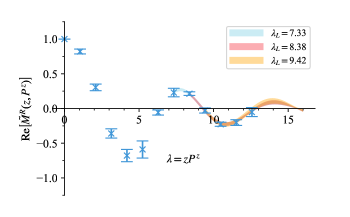
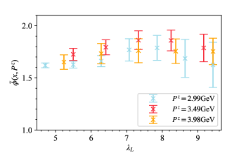
Figure 14: Upper panel: Comparison of the $\lambda_{L}$ dependence of the real part of $\tilde{M}^{R}(z,P^{z})$ at $P^{z}=3.98$GeV. The extrapolated results with $\lambda_{L}=\{7.33,~{}8.38,~{}9.42\}$ are consistent with each other, with only differences in errors. Lower panel: The $\lambda_{L}$ dependence of the quasi DAs $\tilde{\phi}(x,P^{z})$ at fixed $x=0.25$ and $P^{z}=3.98$GeV, which come from the Fourier transformation of extrapolated MEs with different $\lambda_{L}$.

After the extrapolation, we then Fourier transform the extrapolated MEs into momentum space to obtain the quasi DA $\tilde{\phi}(x,P^{z})$ using

$$\tilde{\phi}(x,P^{z})=\int_{-\infty}^{+\infty}\frac{dz}{2\pi}e^{-ixP^{z}z}\tilde{M}^{R}(z,P^{z}).$$ (44)

The numerical results for $\tilde{\phi}(x,P^{z})$ at various $P^{z}$ values are presented in Figure 15. It is crucial to emphasize that the extrapolation formula given by Eq.(43) is formulated based on the behavior of the light-cone distribution at the endpoints as $x$ tends towards 0 and 1. This specifically pertains to the small-$x$ region, where $x$ is roughly less than $1/\lambda_{L}$.

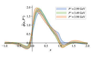
Figure 15: Quasi DAs $\tilde{\phi}(x,P^{z})$ with boosted momenta $P^{z}=\{2.99,3.49,3.98\}$GeV.

IV.3 Matching the quasi DAs to QCD LCDAs

Applying the matching relation given in Eq. (11), we can establish the connection between the renormalized quasi DA $\tilde{\phi}(x,P^{z})$ and the QCD LCDA $\phi(y,\mu)$ at next-to-leading order in $\alpha_{s}$. In order to perform the matching between the quasi DA and the QCD LCDA in the $\overline{\mathrm{MS}}$ scheme, which characterized by the scale $\mu_{0}=2yP^{z}$ or $2\bar{y}P^{z}$, it is essential to resum the large logarithmic terms $\sim\log\left[(2yP^{z})^{2}/\mu^{2}\right]$ and $\log\left[(2\bar{y}P^{z})^{2}/\mu^{2}\right]$ arising in the endpoint region of $y$ to all orders in perturbation theory.

Note that the counterterm in hybrid-ratio scheme does not contain any logarithm, and thus the $\mu$-dependence of the inverse matching coefficient $C^{-1}$ is same as the QCD LCDA $\phi(y,\mu)$ , and the renormalized quasi DA is independent of $\mu$. Therefore, we resum the large logarithms by using the renormalization group equation of the inverse matching coefficient:

$$\frac{dC^{-1}(x,y,P^{z},\mu)}{d\ln\mu^{2}}=\int_{0}^{1}d\zeta V\left[\zeta,y,\alpha_{s}(\mu)\right]C^{-1}(x,\zeta,P^{z},\mu),$$ (45)

which is same as the evolution of $\phi(y,\mu)$. $V\left[\zeta,y,\alpha_{s}(\mu)\right]$ is the Efremov-Radyushkin- Brodsky-Lepage (ERBL) evolution kernel Efremov:1979qk ; Lepage:1980fj of the QCD LCDA which has been calculated up to three loops Braun:2017cih . It is important to note that this evolution process is carried out for the momentum fraction $y$ within $\phi(y,\mu)$, as opposed to the momentum fraction $x$ within $\tilde{\phi}(x,P^{z})$.

By solving Eq.(45) we can obtain the RGR matching kernel $C^{\mathrm{RGR}}(x,y,P^{z},\mu)$ at $\overline{\mathrm{MS}}$ scale $\mu$. We choose $\mu=m_{D}$ to satisfy both the factorization scale of quasi DA, and the renormalization scale of QCD LCDA. Given the uncertainty associated with the initial resummation scale, we systematically vary the scale $\mu_{0}$ to assess the robustness of the perturbative matching procedure and to estimate the pertinent systematic uncertainties, following a similar approach detailed in Sec. IV.1. The selection of different resummation scales captures higher-order effects in $\alpha_{s}$, which are expected to vanish when the perturbative calculation is extended to all orders.

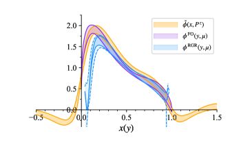
Figure 16: Quasi DA $\tilde{\phi}(x,P^{z})$ with $P^{z}=3.98$GeV, and matched QCD LCDAs from NLO kernel with fixed-order perturbation theory $\phi^{\mathrm{FO}}(y,\mu)$ and RGR improvement $\phi^{\mathrm{RGR}}(y,\mu)$. The scale $\mu$ is chosen as $m_{D}$. The first two results only contain statistical errors, while the latter one not only contains statistical error (solid lines in the blue band), but also the systematic error arising from the scale variation (dashed lines).

Fig. 16 presents a comparison between the quasi distribution amplitude $\tilde{\phi}(x,P^{z})$ at $P^{z}=3.98$ GeV, and the QCD LCDAs obtained from matching with fixed-order perturbation theory, denoted as $\phi^{\mathrm{FO}}(y,\mu)$, and with the RGR improvement, denoted as $\phi^{\mathrm{RGR}}(y,\mu)$. The RGR improvement is performed on both endpoint regions at $y\to 0$ and $y\to 1$. The dashed lines in $\phi^{\mathrm{RGR}}(y,\mu)$ represent the variation of the resummation scale from $0.8\mu_{0}$ to $1.2\mu_{0}$, corresponding to approximately a $20\%$ change in the strong coupling constant $\alpha_{s}(\mu_{0})$ around $y\sim 0.2$. In the intermediate $y$ region, where the physical scale of the quasi distribution amplitude $\mu_{0}$ is in proximity to the $\overline{\mathrm{MS}}$ scale $\mu=m_{D}$ and the resummed logarithms are not excessively large, the RGR-improved and fixed-order matched QCD LCDAs exhibit a high degree of consistency.

In the small $y$ region, such as $0.1\lesssim y\lesssim 0.3$, a significant discrepancy between the two distributions is apparent, indicating the increasing importance of the resummation effect which enhances the accuracy of the theoretical predictions. Additionally, at the endpoint where $y\lesssim 0.1$ and $y\gtrsim 0.9$, the sharp change in behavior observed in $\phi^{\mathrm{RGR}}(y,\mu)$ is attributed to the emergence of the Landau pole, signifying the breakdown of perturbative matching in this region.

Moreover, it is important to note that the resummation of logarithmic terms from higher orders can disrupt the normalization of the QCD LCDAs at fixed order. Specifically, we observe that $\int_{0}^{1}dy\phi^{\mathrm{FO}}(y,\mu)=1\neq\int_{0}^{1}dy\phi^{\mathrm{RGR}}(y,\mu)$ in Fig. 16. A similar normalization problem also exists in the analysis of QCD LCDAs from the matching of HQET LCDAs Beneke:2018wjp . To address this issue, we have determined that the central values of the QCD LCDAs obtained from the RGR-improved matching kernel are typically normalized to around 0.81. Consequently, we rescale the QCD LCDA $\phi^{\mathrm{RGR}}(y,\mu)$ to ensure its normalization to 1 for subsequent phenomenological analyses.

In Fig. 17, we present the $P^{z}$-dependence of the QCD LCDA with RGR-improved NLO matching. The momenta of the boosted heavy meson are selected as $P^{z}=\{6,~{}7,~{}8\}\times 2\pi/L\simeq\{2.99,~{}3.49,~{}3.98\}$ GeV. Our analysis reveals that the results at different $P^{z}$ values exhibit consistent behavior within the margins of error, suggesting a potential saturation at large momenta which needs more detailed analysis in the future. Given the consistency across various momenta, we opt to utilize the result obtained at $P^{z}=3.98$ GeV as our final prediction for the QCD LCDA , and compute the systematic error arising from power corrections at finite $P^{z}$ by comparing the central value of the result at $P^{z}=3.98$GeV with that at $P^{z}=2.99$GeV.

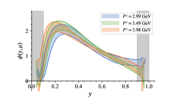
Figure 17: The $P^{z}$ dependence of the QCD LCDAs. Only statistic error and systematic error from scale variation in RGR are included in the error bands. The grey band indicates the region ($y\lesssim\Lambda_{\mathrm{QCD}}/P^{z}\simeq 0.1$) where the matching in LaMET failed.

IV.4 Determination of HQET LCDA

As discussed in Sec. II.2, we extract the peak region of the HQET LCDA from the QCD LCDA using a multiplicative factorization approach. The resulting matched HQET LCDA is depicted by the red band in Fig. 18. From this figure, one can observe that the peak position of the QCD LCDA $\phi(y,\mu=m_{D})$ (orange band) is situated within the range $y\in[0.2,0.3]$, corresponding to the scenario where the light quark carries a typical light-cone momentum fraction $y\sim\Lambda_{\mathrm{QCD}}/m_{D}$. Furthermore, at very large scales $\mu\gg m_{D}$, the QCD LCDA reverts back to its asymptotic form akin to that of a light meson.

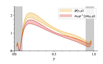
Figure 18: Comparison of QCD LCDA and HQET LCDA obtained from matching via Eq.(19) at $\mu=m_{D}$. Only statistic errors are obtained in both results. It should be noted that although the full distribution of HQET LCDA is shown, only the part satisfies $\omega\sim\Lambda_{\mathrm{QCD}}$ is valid.

Before reaching a final conclusion regarding the peak region, we address potential sources of systematic errors in our analysis, which may arise from

• the extrapolation of long-range correlations. We use the data with $\lambda\geq\lambda_{L}$ for the fit, and vary the values of $\lambda_{L}$ from $\{7.07,~{}7.33,~{}7.33\}$ to $\{9.42,~{}9.16,~{}9.42\}$ (for the renormalized MEs at $P^{z}=\{2.99,3.49,3.98\}$GeV) to estimate the systematic error.

• the scale uncertainty of the MEs renormalized in hybrid-ratio scheme. In the process of matching from lattice results to the light-cone quantities in the $\overline{\mathrm{MS}}$ scheme, uncertainties in the initial conditions can introduce systematic errors. In the renormalization group running of the Wilson coefficient discussed in Sec. IV.1, we adopt an initial condition for scale evolution of $c^{\prime}\times 2e^{-\gamma_{E}}z^{-1}$, while in the renormalization group running of the perturbative matching kernel as discussed in Sec. IV.3, we use $c^{\prime}\times 2xP^{z}$. To assess the impact of these initial conditions, we vary the factor $c^{\prime}$ in the range of 0.8 to 1.2 to estimate the systematic error.

• the difference between QCD LCDAs extracted at different large $P^{z}$. Rather than extrapolating $P^{z}$ to infinite momentum, we adopt the QCD LCDA result at $P^{z}=3.98$ GeV as our final prediction. To quantify the systematic error, we calculate the difference between this prediction and the one at $P^{z}=2.99$ GeV.

Combining the statistical and systematic errors discussed earlier, we derive the numerical results for the heavy meson HQET LCDA from lattice QCD through a two-step matching process, which contributes to the peak region of the final prediction. The results are shown in Fig.19, in which the band represented by dashed lines corresponds to the result including only statistical errors, while the one with solid lines represents the result incorporating both statistical and systematic errors.

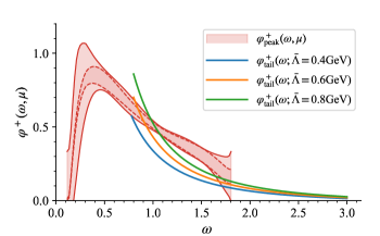
Figure 19: The result of HQET LCDA in the peak region $\varphi_{\mathrm{peak}}^{+}(\omega,\mu)$ and in the tail region $\varphi_{\mathrm{tail}}^{+}(\omega;\bar{\Lambda})$. The dashed lines in $\varphi_{\mathrm{peak}}^{+}(\omega,\mu)$ indicate the upper and lower limits of the result containing only statistical error, while the solid lines indicate the result including both statistical and systematic errors. Three colored solid lines of $\varphi_{\mathrm{tail}}^{+}(\omega;\bar{\Lambda})$ represent the results at $\bar{\Lambda}=\{0.4,0.6,0.8\}$GeV, where $\bar{\Lambda}$ denotes the power corrections in the perturbative calculations.

The tail region of HQET LCDA contains only hard-collinear contributions, which would contribute only through power corrections. We employ the one-loop level result from Ref. Lee:2005gza that is given in Eq. (18). The parameter $\bar{\Lambda}$ reflects the power correction and usually be chosen at hundreds of MeV. Here we use $\bar{\Lambda}=\{0.4,\,0.6,\,0.8\}$GeV to estimate the power correction in Eq.(18), shown as the colored lines in Fig.19.

The power counting of parameters in HQET LCDA reveals that the momentum of the light quark in the peak region satisfies $\omega\sim\mathcal{O}(\Lambda_{\mathrm{QCD}})$, while in the tail region it satisfies $\omega\sim\mathcal{O}(m_{D})$. This suggests that the boundary between them lies in the range $\Lambda_{\mathrm{QCD}}\ll\omega_{b}\ll m_{D}$. From Fig. 19, we observe that the intersection of the peak and tail regions occurs around 0.9 GeV, confirming the aforementioned statement. Consequently, we merge them into a continuous distribution with

$$\varphi^{+}(\omega,\mu)=\varphi^{+}_{\mathrm{peak}}(\omega,\mu)\theta(\omega_{b}-\omega)+\varphi^{+}_{\mathrm{tail}}(\omega,\mu)\theta(\omega-\omega_{b}),$$ (46)

where the intersection position $\omega_{b}=\{0.79,~{}0.87,~{}0.96\}$GeV for $\bar{\Lambda}=\{0.4,~{}0.6,~{}0.8\}$GeV. In order to ensure a smooth transition between the peak and tail regions, we utilize a polynomial filter, specifically the Savitzky-Golay filter, on the results within a vicinity of $\delta=0.05$ GeV around $\omega_{b}$ to smoothen the curve.

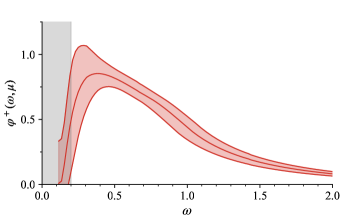
Figure 20: Final result of HQET LCDA $\varphi^{+}(\omega,\mu)$ at $\mu=m_{D}$. All statistical and systematic errors are included. The grey band indicates the region where our result suffers significant power corrections, approximately in $\omega\lesssim 0.19$GeV.

The combined result of the peak and tail regions is illustrated in Fig. 20. The peak region is derived from lattice QCD calculations and encompasses both statistical and systematic errors, while the tail region is determined from one-loop perturbation theory and includes solely systematic errors. The grey band highlights the range where our findings are notably affected by power corrections, specifically around $\omega\lesssim 0.19$ GeV.

V Phenomenological discussions

V.1 Tabulated results for HQET LCDA

We present the numerical results of the peak region of HQET LCDA $\varphi^{+}_{\mathrm{peak}}(\omega,\mu)$ in Tab.2, which are determined from lattice QCD calculations. As mentioned earlier, in the small $\omega$ region ($\omega\sim m_{D}\Lambda_{\mathrm{QCD}}/P^{z}$), the results are affected by significant power corrections, while in the large $\omega$ region ($\omega\gg\Lambda_{\mathrm{QCD}}$), the HQET LCDA prediction relies on perturbative calculations. Therefore, we present the numerical results for the HQET LCDA $\varphi^{+}(\omega,\mu)$ in the peak region with $\omega\in[0.192,~{}0.806]$ GeV. These results include the central values $\overline{\varphi^{+}_{\mathrm{peak}}(\omega,\mu)}$ and the covariance matrix $\mathrm{Cov}(\varphi^{+}_{\mathrm{peak}}(\omega,\mu))$ associated with different $\omega$ values. The renormalization scale $\mu$ is chosen to be the charmed meson mass $m_{D}$.

Table 2: Numerical results for the HQET LCDA $\varphi^{+}(\omega,\mu)$ at ranging $\omega\in[0.192,~{}0.806]$GeV, including the central value $\overline{\varphi^{+}_{\mathrm{peak}}(\omega,\mu)}$ and covariant matrix $\mathrm{Cov}(\varphi^{+}_{\mathrm{peak}}(\omega,\mu))$ (in units of $10^{-3}$). The non-diagonal terms in the covariant matrix come from the correlations between different gauge ensembles. The renormalization scale $\mu$ is chosen to be $m_{D}$.

$\omega$ (GeV)	0.192	0.269	0.346	0.422	0.499	0.576	0.653	0.73	0.806
$\overline{\varphi^{+}_{\mathrm{peak}}(\omega,\mu)}$	0.458	0.779	0.868	0.869	0.839	0.793	0.742	0.689	0.637
	158.9	0.941	1.125	1.157	1.095	0.967	0.796	0.601	0.394
	0.941	98.6	2.325	2.450	2.334	2.051	1.662	1.220	0.762
	1.125	2.325	33.38	3.266	3.138	2.761	2.228	1.618	0.993
$\mathrm{Cov}(\varphi^{+}_{\mathrm{peak}}(\omega,\mu))$	1.157	2.450	3.266	10.86	3.450	3.060	2.489	1.828	1.144
(in units of $10^{-3}$)	1.095	2.334	3.138	3.450	5.538	3.037	2.513	1.890	1.233
	0.967	2.051	2.761	3.060	3.037	4.635	2.352	1.829	1.261
	0.796	1.662	2.228	2.489	2.513	2.352	4.771	1.668	1.226
	0.601	1.220	1.618	1.828	1.890	1.829	1.668	4.582	1.128
	0.394	0.762	0.993	1.144	1.233	1.261	1.226	1.128	3.764

V.2 Comparison with phenomenological models

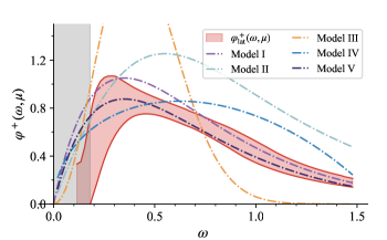
Figure 21: Comparison of the numerical results of $\varphi^{+}\left(\omega,\mu\right)$ from lattice QCD with several commonly used phenomenological models in Eq.(47). The renormalization scale $\mu$ of our result is chosen to be $m_{D}$. We only show the central values of the models as colored dashed lines, and interpret their spread as error estimate.

Table 3: Our results of the parameters by fitting the models in Eq.(47) compare to those values given in references Wang:2015vgv ; Beneke:2018wjp ; Gao:2021sav . Due to the unique behavior of model III, we are unable to obtain a good fit using this model ($\chi^{2}/$d.o.f$>$2 and the fitted results are unable to describe the data). When fitting model V, we adopt the values for parameters $\alpha$ and $\beta$ from Ref. Beneke:2018wjp ; Gao:2021sav .

Models	I	II	III	IV	V
This work	$\omega_{0}=444\pm 60$MeV	$\omega_{0}=630\pm 133$MeV	———	$\omega_{0}=365\pm 33$MeV	$\omega_{0}=439\pm 59$MeV
		$\sigma_{B}^{(1)}=2.54\pm 1.89$GeV
References	$\omega_{0}=354_{-30}^{+38}$MeV	$\omega_{0}=368_{-32}^{+42}$MeV	$\omega_{0}=389_{-28}^{+35}$MeV	$\omega_{0}=303_{-26}^{+35}$MeV	$\omega_{0}=350$MeV
		$\sigma_{B}^{(1)}=1.4\pm 0.4$GeV

In this subsection, we will compare our results for the HQET LCDA with those from previous studies based on various phenomenological models Grozin:1996pq ; Braun:2003wx ; Beneke:2018wjp :

$$\varphi_{\mathrm{I}}^{+}\left(\omega,\mu_{0}\right)=\frac{\omega}{\omega_{0}^{2}}e^{-\omega/\omega_{0}},$$

$$\varphi_{\mathrm{II}}^{+}\left(\omega,\mu_{0}\right)=\frac{4}{\pi\omega_{0}}\frac{k}{k^{2}+1}\left[\frac{1}{k^{2}+1}-\frac{2\left(\sigma_{B}^{(1)}-1\right)}{\pi^{2}}\ln k\right],$$

$$\varphi_{\mathrm{III}}^{+}\left(\omega,\mu_{0}\right)=\frac{2\omega^{2}}{\omega_{0}\omega_{1}^{2}}e^{-\left(\omega/\omega_{1}\right)^{2}},$$

$$\varphi_{\mathrm{IV}}^{+}\left(\omega,\mu_{0}\right)=\frac{\omega}{\omega_{0}\omega_{2}}\frac{\omega_{2}-\omega}{\sqrt{\omega\left(2\omega_{2}-\omega\right)}}\theta\left(\omega_{2}-\omega\right),$$

$$\varphi_{\mathrm{V}}^{+}(\omega,\mu_{0})=\frac{\Gamma(\beta)}{\Gamma(\alpha)}\frac{\omega}{\omega_{0}^{2}}e^{-\omega/\omega_{0}}U(\beta-\alpha,3-\alpha,\omega/\omega_{0}).$$ (47)

The parameters of the first four models are collected as follows Wang:2015vgv : in model I, $\omega_{0}=354_{-30}^{+38}$MeV; in model II, $\omega_{0}=368_{-32}^{+42}$MeV, $\sigma_{B}^{(1)}=1.4\pm 0.4$GeV and $k={\omega}/{1\,\mathrm{GeV}}$; in model III, $\omega_{0}=389_{-28}^{+35}$MeV and $\omega_{1}={2\omega_{0}}/{\sqrt{\pi}}$; in model IV, $\omega_{0}=303_{-26}^{+35}$MeV and $\omega_{2}={4\omega_{0}}/{(4-\pi)}$. These parameters are all given at $\mu=1$GeV. In model V, $U(a,b,z)$ denotes the second kind confluent hypergeometric function, and the parameters $\omega_{0}$, $\alpha$ and $\beta$ can be solved from the numerical results of $\lambda_{B}$ and $\hat{\sigma}_{1}$ Beneke:2018wjp ; Gao:2021sav .

In Fig. 21, we compare our results with those parametrized in Eq. (47). To avoid cluttering the plot and due to the challenges in estimating uncertainties in model-based analyses, we only display the central values as colored dashed lines. The spread of these lines serves as an estimate of systematic errors in the models, and we refrain from discussing the relative merits of these different models. It is worth noting that while our results are consistent with the combined phenomenological model estimates, they exhibit better theoretical foundation. The analysis in this study was primarily intended as a demonstration. We are confident that future lattice simulations following similar methodologies will significantly improve precision, possibly eliminating the necessity for model-based analyses.

Furthermore, we have conducted data fitting based on the models outlined in Eq.(47), and the corresponding results are detailed in Table 3. The fit range is selected based on the range that yields the optimal quality of fit to the data. Due to the unique behavior of model III, we are unable to obtain a good fit using this model ($\chi^{2}/$d.o.f$>$2 and the fitted results are unable to describe the data). When fitting model V, we adopt the parameter values for $\alpha$ and $\beta$ as specified in Ref. Beneke:2018wjp ; Gao:2021sav , which are not significantly influenced by the data. Notably, in these models, the parameter $\omega_{0}$ is equivalent to $\lambda_{B}$.

V.3 Determination of the inverse and inverse-logarithmic moments

The first inverse moment $\lambda_{B}^{-1}$ and inverse-logarithmic moments $\sigma_{B}^{(n)}$ play a pivotal role in QCD factorization theorems and lightcone sum rule studies in heavy flavor physics. These quantities are defined as:

$$\lambda_{B}^{-1}(\mu)= \int_{0}^{\infty}\frac{d\omega}{\omega}\varphi^{+}(\omega,\mu),$$ (48)

$$\sigma^{(n)}_{B}(\mu)= \lambda_{B}(\mu)\int_{0}^{\infty}\frac{d\omega}{\omega}\ln\left(\frac{\mu}{\omega}\right)^{(n)}\varphi^{+}(\omega,\mu).$$ (49)

While the first inverse moment $\lambda_{B}^{-1}$ and the first inverse-logarithmic moments $\sigma_{B}^{(1)}$ have been estimated in various approaches Belle:2018jqd ; Khodjamirian:2020hob ; Lee:2005gza ; Braun:2003wx ; Grozin:1996pq , there is considerable scope for enhancing their reliability and precision. In the case of $\sigma^{(2)}_{B}$ and subsequent orders, no existing results are currently available.

To determine these values from the HQET LCDA we have developed, it is essential to integrate the HQET LCDA $\varphi^{+}(\omega,\mu)$ over $\omega$ from 0 to infinity. As noted earlier, our results will be influenced by significant power corrections at low $\omega$, presenting difficulties for accurate predictions in this regime. Alternatively, we can employ a model-independent parametrization formula to extrapolate our results towards the region near $\omega=0$. For small $\omega$, an expansion can be expressed as:

$$\varphi^{+} \left(\omega,\mu\right)=\sum_{n=1}^{N}c_{n}\frac{\omega^{n}}{\omega_{0}^{n+1}}e^{-\omega/\omega_{0}}$$

$$= \frac{c_{1}\omega}{\omega_{0}^{2}}\left[1+c_{2}^{\prime}\frac{\omega}{\omega_{0}}+c_{3}^{\prime}\left(\frac{\omega}{\omega_{0}}\right)^{2}+\cdots\right]e^{-\omega/\omega_{0}},$$ (50)

with $c_{n}^{\prime}\equiv c_{n}/c_{1}$. One benefit of this parametrization is that for small $\omega\ll\omega_{0}$, higher moments become less influential. By expanding Eq.(50) up to the first ($N=1$), second ($N=2$), and third ($N=3$) order terms, we can determine the parameters as:

$$N=1:~{} \omega_{0}=0.403(44),~{}c_{1}=0.932(73);$$

$$N=2:~{} \omega_{0}=0.352(82),~{}c_{1}=0.69(37),$$

$$c_{2}^{\prime}=0.17(32);$$

$$N=3:~{} \omega_{0}=0.32(15),~{}c_{1}=0.63(44),$$

$$c_{2}^{\prime}=0.12(37),c_{3}^{\prime}=0.04(19).$$ (51)

The outcomes derived using the aforementioned parameters are illustrated in Fig. 22. It is evident that the results obtained from expanding to the $N$-th order ($N=1,~{}2,~{}3$) exhibit consistency, signifying the favorable convergence of the expansion depicted in Eq.(50).

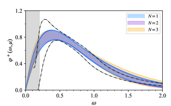
Figure 22: Fit results of the model-independent parametrization in Eq.(50) up to the $N$-th order. The fitting range adopted is $\omega\in[0.192,0.806]$GeV. The dashed lines indicate the upper and lower limits of the original data.

Using the extrapolated data, we can evaluate the integrals in Eq.(49) to determine the numerical values of the first inverse moment $\lambda_{B}^{-1}$ and the first two inverse-logarithmic moments $\sigma_{B}^{(1,2)}$ of the HQET LCDA. These results are displayed in the upper panel of Table 4, where $N$ denotes the truncation order in the expansion of Eq.(49). Note that these results are obtained at $\mu=m_{D}$ through fitting the data in Tab.2. To evolve them to the soft scale $\mu=1$ GeV, which is commonly used in phenomenology, we adopt the following RG evolution equations Wang:2015vgv

$$\frac{\lambda_{B}\left(\mu_{0}\right)}{\lambda_{B}(\mu)}= 1+\frac{a_{s}(\mu_{0})}{4}\ln\frac{\mu}{\mu_{0}}\left[2-2\ln\frac{\mu}{\mu_{0}}-4\sigma_{B}^{(1)}\left(\mu_{0}\right)\right]$$

$$\qquad+\mathcal{O}\left(a_{s}^{2}\right),$$ (52)

$$\sigma_{B}^{(1)}(\mu)= \sigma_{B}^{(1)}\left(\mu_{0}\right)+\ln\frac{\mu}{\mu_{0}}\bigg{(}1+a_{s}(\mu_{0})$$

$$\qquad\times\left[\left(\sigma_{B}^{(1)}\left(\mu_{0}\right)\right)^{2}-\sigma_{B}^{(2)}\left(\mu_{0}\right)\right]\bigg{)}+\mathcal{O}\left(a_{s}^{2}\right).$$ (53)

Here $a_{s}(\mu)\equiv\alpha_{s}(\mu)C_{F}/\pi$. The results of $\lambda_{B}$ and $\sigma_{B}^{(1)}$ after RG evolution are collected in the central panel of Table 4. The values of $\sigma_{B}^{(2)}$ is not included because its evolution depends on the value of $\sigma_{B}^{(3)}$ at $\mu=m_{D}$. There is no phenomenological estimate for them at this stage.

Table 4: Upper panel: Numerical results for $\lambda_{B}$ and $\sigma_{B}^{(1,2)}$ at $\mu=m_{D}$, which are obtained from the fits based on Eq.(50) up to the $N$-th order. Central panel: Results of $\lambda_{B}$ and $\sigma_{B}^{(1)}$ at $\mu=1$GeV after RG evolution, which is consistent with the scale of theoretical results rpesented in the lower panel. Lower panel: $\lambda_{B}$ and $\sigma_{B}^{(1)}$ from experiment and other theoretical approaches.

$\mu$		$\lambda_{B}$ (GeV)	$\sigma_{B}^{(1)}$	$\sigma_{B}^{(2)}$
	$N=1$	0.433(39)	2.14(11)	6.20(46)
$m_{D}$	$N=2$	0.437(41)	2.13(10)	6.14(43)
	$N=3$	0.424(65)	2.15(15)	6.21(81)
	$N=1$	0.389(35)	1.63(8)
1GeV	$N=2$	0.393(37)	1.62(7)
	$N=3$	0.381(59)	1.63(12)
	Ref.Belle:2018jqd	$>0.24$
	Ref.Khodjamirian:2020hob	$0.383(153)$
1GeV	Ref.Lee:2005gza	$0.48(11)$	$1.6(2)$
	Ref.Braun:2003wx	$0.46(11)$	$1.4(4)$
	Ref.Grozin:1996pq	$0.35(15)$
	Ref. Gao:2019lta	$0.343^{+0.064}_{-0.079}$
	Ref.Mandal:2023lhp	$0.338(68)$

For a comparison, we present the results of inverse and inverse-logarithmic moments from experimental data and other theoretical approaches in the lower panel of Table 4. Using the measurement of $B\to\gamma\ell\nu$, the Belle collaboration has provided a lower bound of $\lambda_{B}>0.24$ GeV at a $90\%$ confidence level Belle:2018jqd . Further constraints on $\lambda_{B}$ Khodjamirian:2020hob ; Braun:2003wx ; Grozin:1996pq and $\sigma_{B}^{(1)}$ Braun:2003wx are derived from QCD sum rules. Additionally, Ref. Lee:2005gza offers results for $\lambda_{B}$ and $\sigma_{B}^{(1)}$ using a realistic model description of the B-meson LCDA. In Ref.Mandal:2023lhp , $\lambda_{B}$ is extracted by fitting the lattice results of the $B\to K$ form factors.

Comparing the results presented in Table 4, we observe that our findings for $\lambda_{B}$ are in agreement with those derived from experimental data and other theoretical methods. While the results for $\sigma_{B}^{(1)}$ are only available from certain theoretical studies, it is notable that our results are still in approximate agreement with them after performing the scale evolution.

V.4 Impact on $B\to V$ form factors

In Ref. Gao:2019lta , the $B\to V$ form factors have been updated in LCSRs using $B$-meson light-cone distribution amplitudes. In addition to the next-to-leading order QCD corrections, the light-quark mass effect for the local soft-collinear effective theory form factors is also computed from the LCSR method. Furthermore, the subleading power corrections to $B\to V$ form factors from the higher-twist B-meson light-cone distribution amplitudes are also computed with the same method at tree level up to the twist-six accuracy.

Instead of the ordinary form factors, the authors of Ref. Gao:2019lta have calculated the following form factors:

$${\cal V}(q^{2})= \frac{m_{B}}{m_{B}+m_{V}}V(q^{2}),$$

$${\cal A}_{0}(q^{2})= \frac{m_{V}}{E_{V}}A_{0}(q^{2}),$$

$${\cal A}_{1}(q^{2})= \frac{m_{B}+m_{V}}{2E_{V}}A_{1}(q^{2}),$$

$${\cal A}_{12}(q^{2})= \frac{m_{B}+m_{V}}{2E_{V}}A_{1}(q^{2})-\frac{m_{B}-m_{V}}{m_{B}}A_{2}(q^{2}),$$

$${\cal T}_{1}(q^{2})= T_{1}(q^{2}),$$

$${\cal T}_{2}(q^{2})= \frac{m_{B}}{2E_{V}}T_{2}(q^{2}),$$

$${\cal T}_{23}(q^{2})= {\cal T}_{2}(q^{2})-T_{3}(q^{2}),$$ (54)

where $m_{V}$ and $E_{V}$ denote the mass and energy for the vector meson, respectively. $m_{B}$ is the $B$ meson mass. At $q^{2}=0$, ${\cal A}_{0}(0)={\cal A}_{12}(0)$ and ${\cal T}_{1}(0)={\cal T}_{2}(0)$.

Using these analytical results, we present the dependence of the $B\to K^{*}$ form factors on the first inverse moment in Fig. 23. In alignment with the conventions of Ref. Gao:2019lta , we have adopted the results for $N=1$. Given that ${\cal V}$, ${\cal T}_{1}$, and ${\cal A}_{1}$ exhibit very similar numerical values, we have chosen to only display the results for ${\cal V}$ and ${\cal A}_{0},{\cal T}_{23}$ at $q^{2}=0$. The band labeled as “GLSWW” represents the results obtained using the inverse moment directly from Ref. Gao:2019lta , as shown in Eq. 55. On the other hand, the band labeled as “This work” corresponds to the inverse moment calculated in this paper. It is important to mention that in Ref. Gao:2019lta , the exponential model for the $B$ meson LCDAs utilizes the first inverse moment as:

$$\lambda_{B}=(0.343^{+0.064}_{-0.079}){\rm GeV}.$$ (55)

This value is obtained by matching the results for $B\to\rho$ form factors onto the QCD LCSRs using light meson LCDAs.

From Fig. 23, we can see that the form factors computed using our inverse moment are in agreement with those in Ref. Gao:2019lta , although it should be stressed that systematic uncertainties are not included in this paper. From the results for ${\cal V}^{B\to K^{*}}(0)$ in Eq. I, one can observe that a precise determination of $\lambda_{B}$ can lead to an accurate prediction. More importantly, our results from first-principles of QCD help to remove the primary uncertainties arising from the model parametrizations of heavy meson LCDAs. This indicates the potential for a more precise analysis of form factors and accordingly physical observables, like the determination of $|V_{ub}|$.

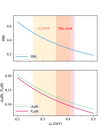
Figure 23: The dependence of the $B\to K^{*}$ form factors on the inverse moment of heavy meson LCDAs in the exponential model based on the results in Ref. Gao:2019lta . The band labeled as “GLSWW” represents the results obtained using the inverse moment directly from Ref. Gao:2019lta , as shown in Eq. 55. On the other hand, the band labeled as “This work” corresponds to the inverse moment calculated in this paper.

VI Summary

In this study, a unique framework for determining HQET LCDAs through a sequential effective theory approach is introduced and elaborated upon. The theoretical underpinnings of the framework have been discussed, providing a comprehensive overview of the methodology. We have then delved into the intricacies of lattice QCD simulations, emphasizing the importance of analyzing dispersion relations and implementing fitting strategies to extract meaningful results. The calculations of quasi DAs, QCD LCDAs, and HQET LCDAs are showcased, offering valuable insights into the structure and behavior of heavy quark systems. Discussions focuses on the potential phenomenological implications of the findings, highlighting the implications for future research in the field of high-energy physics. The potential phenomenological implications of the results are explored, offering insights into how these findings could influence our comprehension of the dynamics of strong and weak interactions.

It should be emphasized that the current results are based on the simulation of quasi DAs with a single lattice spacing and perturbative calculation at leading power, where the predictions are likely to be affected by various systematic uncertainties from both lattice and analytical sides. In the future, there are several areas of research that can be explored to further advance our understanding of heavy quark systems through the framework of HQET LCDAs using a sequential effective theory approach. Here are some potential avenues for future investigation.

• Building upon the framework of heavy quark spin symmetry, delving into the properties and behaviors of heavy vector mesons within the context of HQET LCDAs could yield valuable insights into the dynamics of these systems. Exploring their quasi-distribution amplitudes and QCD local distribution amplitudes can deepen our comprehension of the structure of heavy quark systems.

• Utilizing smaller lattice spacings and larger momentum values in lattice QCD simulations can help improve the accuracy and precision of our calculations. Together with the investigation of lattice artifacts such as operator mixing effects, they can lead to more reliable results and a better understanding of the behavior of heavy quark systems at different energy scales.

• Exploring a wider range of masses for the heavy quark and studying their dependence on various parameters can provide a more comprehensive picture of the behavior of heavy quark systems. This can help elucidate the effects of mass on the structure and dynamics of these systems. An analysis using different heavy quark mass is under progress.

• The perturbative results employed in this study are at the next-to-leading order in $\alpha_{s}$. Accounting for higher-order or instance two-loop corrections has the potential to substantially diminish the associated uncertainties. This involves the perturbative calculation of two-loop matching kernels in two steps, and the HQET LCDAs in the endpoint region.

• Our current focus is mainly on $\varphi_{B}^{+}(\omega)$, while investigating the function $\varphi_{B}^{-}(\omega)$, which describes another leading-power distribution amplitudes of heavy quark systems, can offer valuable insights into the internal structure and properties of these systems. Understanding the behavior of $\varphi^{-}(\omega)$ can also help refine our theoretical framework and improve our theoretical predictions.

By exploring these areas of research in the future, we can further enhance our understanding of heavy quark systems and advance the field of high-energy physics.

References

- (1) A. G. Grozin and M. Neubert, Phys. Rev. D 55, 272-290 (1997) doi:10.1103/PhysRevD.55.272 [arXiv:hep-ph/9607366 [hep-ph]].
- (2) M. Beneke, G. Buchalla, M. Neubert and C. T. Sachrajda, Phys. Rev. Lett. 83, 1914-1917 (1999) doi:10.1103/PhysRevLett.83.1914 [arXiv:hep-ph/9905312 [hep-ph]].
- (3) M. Beneke, G. Buchalla, M. Neubert and C. T. Sachrajda, Nucl. Phys. B 591, 313-418 (2000) doi:10.1016/S0550-3213(00)00559-9 [arXiv:hep-ph/0006124 [hep-ph]].
- (4) Y. Y. Keum, H. N. Li and A. I. Sanda, Phys. Rev. D 63, 054008 (2001) doi:10.1103/PhysRevD.63.054008 [arXiv:hep-ph/0004173 [hep-ph]].
- (5) C. D. Lu, K. Ukai and M. Z. Yang, Phys. Rev. D 63, 074009 (2001) doi:10.1103/PhysRevD.63.074009 [arXiv:hep-ph/0004213 [hep-ph]].
- (6) B. O. Lange and M. Neubert, Phys. Rev. Lett. 91, 102001 (2003) doi:10.1103/PhysRevLett.91.102001 [arXiv:hep-ph/0303082 [hep-ph]].
- (7) S. J. Lee and M. Neubert, Phys. Rev. D 72, 094028 (2005) doi:10.1103/PhysRevD.72.094028 [arXiv:hep-ph/0509350 [hep-ph]].
- (8) H. Kawamura and K. Tanaka, Phys. Lett. B 673, 201-207 (2009) doi:10.1016/j.physletb.2009.02.028 [arXiv:0810.5628 [hep-ph]].
- (9) G. Bell, T. Feldmann, Y. M. Wang and M. W. Y. Yip, JHEP 11, 191 (2013) doi:10.1007/JHEP11(2013)191 [arXiv:1308.6114 [hep-ph]].
- (10) T. Feldmann, B. O. Lange and Y. M. Wang, Phys. Rev. D 89, no.11, 114001 (2014) doi:10.1103/PhysRevD.89.114001 [arXiv:1404.1343 [hep-ph]].
- (11) V. M. Braun, Y. Ji and A. N. Manashov, Phys. Rev. D 100, no.1, 014023 (2019) doi:10.3204/PUBDB-2019-02451 [arXiv:1905.04498 [hep-ph]].
- (12) Y. M. Wang and Y. L. Shen, Nucl. Phys. B 898, 563-604 (2015) doi:10.1016/j.nuclphysb.2015.07.016 [arXiv:1506.00667 [hep-ph]].
- (13) M. Beneke, V. M. Braun, Y. Ji and Y. B. Wei, JHEP 07, 154 (2018) doi:10.1007/JHEP07(2018)154 [arXiv:1804.04962 [hep-ph]].
- (14) J. Gao, T. Huber, Y. Ji, C. Wang, Y. M. Wang and Y. B. Wei, JHEP 05, 024 (2022) doi:10.1007/JHEP05(2022)024 [arXiv:2112.12674 [hep-ph]].
- (15) V. M. Braun, D. Y. Ivanov and G. P. Korchemsky, Phys. Rev. D 69, 034014 (2004) doi:10.1103/PhysRevD.69.034014 [arXiv:hep-ph/0309330 [hep-ph]].
- (16) J. Lan, C. Mondal, M. Li, Y. Li, S. Tang, X. Zhao and J. P. Vary, Phys. Rev. D 102, no.1, 014020 (2020) doi:10.1103/PhysRevD.102.014020 [arXiv:1911.11676 [nucl-th]].
- (17) A. Khodjamirian, R. Mandal and T. Mannel, JHEP 10, 043 (2020) doi:10.1007/JHEP10(2020)043 [arXiv:2008.03935 [hep-ph]].
- (18) M. Rahimi and M. Wald, Phys. Rev. D 104, no.1, 016027 (2021) doi:10.1103/PhysRevD.104.016027 [arXiv:2012.12165 [hep-ph]].
- (19) F. E. Serna, R. C. da Silveira, J. J. Cobos-Martínez, B. El-Bennich and E. Rojas, Eur. Phys. J. C 80, no.10, 955 (2020) doi:10.1140/epjc/s10052-020-08517-3 [arXiv:2008.09619 [hep-ph]].
- (20) J. Gao, C. D. Lü, Y. L. Shen, Y. M. Wang and Y. B. Wei, Phys. Rev. D 101, no.7, 074035 (2020) doi:10.1103/PhysRevD.101.074035 [arXiv:1907.11092 [hep-ph]].
- (21) B. Y. Cui, Y. K. Huang, Y. L. Shen, C. Wang and Y. M. Wang, JHEP 03, 140 (2023) doi:10.1007/JHEP03(2023)140 [arXiv:2212.11624 [hep-ph]].
- (22) I. A. Korchemskaya and G. P. Korchemsky, Phys. Lett. B 287, 169-175 (1992) doi:10.1016/0370-2693(92)91895-G
- (23) X. Y. Han, J. Hua, X. Ji, C. D. Lü, W. Wang, J. Xu, Q. A. Zhang and S. Zhao, [arXiv:2403.17492 [hep-ph]].
- (24) X. Ji, Phys. Rev. Lett. 110, 262002 (2013) doi:10.1103/PhysRevLett.110.262002 [arXiv:1305.1539 [hep-ph]].
- (25) X. Ji, Sci. China Phys. Mech. Astron. 57, 1407-1412 (2014) doi:10.1007/s11433-014-5492-3 [arXiv:1404.6680 [hep-ph]].
- (26) X. Ji, Y. S. Liu, Y. Liu, J. H. Zhang and Y. Zhao, Rev. Mod. Phys. 93, no.3, 035005 (2021) doi:10.1103/RevModPhys.93.035005 [arXiv:2004.03543 [hep-ph]].
- (27) K. Cichy and M. Constantinou, Adv. High Energy Phys. 2019, 3036904 (2019) doi:10.1155/2019/3036904 [arXiv:1811.07248 [hep-lat]].
- (28) S. Ishaq, Y. Jia, X. Xiong and D. S. Yang, Phys. Rev. Lett. 125, no.13, 132001 (2020) doi:10.1103/PhysRevLett.125.132001 [arXiv:1905.06930 [hep-ph]].
- (29) M. Beneke, G. Finauri, K. K. Vos and Y. Wei, JHEP 09, 066 (2023) doi:10.1007/JHEP09(2023)066 [arXiv:2305.06401 [hep-ph]].
- (30) Z. C. Hu et al. [CLQCD], Phys. Rev. D 109, no.5, 054507 (2024) doi:10.1103/PhysRevD.109.054507 [arXiv:2310.00814 [hep-lat]].
- (31) M. Gelb et al. [Belle], Phys. Rev. D 98, no.11, 112016 (2018) doi:10.1103/PhysRevD.98.112016 [arXiv:1810.12976 [hep-ex]].
- (32) H. Kawamura and K. Tanaka, PoS RADCOR2017, 076 (2018) doi:10.22323/1.290.0076
- (33) W. Wang, Y. M. Wang, J. Xu and S. Zhao, Phys. Rev. D 102, no.1, 011502 (2020) doi:10.1103/PhysRevD.102.011502 [arXiv:1908.09933 [hep-ph]].
- (34) S. Zhao and A. V. Radyushkin, Phys. Rev. D 103, no.5, 054022 (2021) doi:10.1103/PhysRevD.103.054022 [arXiv:2006.05663 [hep-ph]].
- (35) J. Xu, X. R. Zhang and S. Zhao, Phys. Rev. D 106, no.1, L011503 (2022) doi:10.1103/PhysRevD.106.L011503 [arXiv:2202.13648 [hep-ph]].
- (36) J. Xu and X. R. Zhang, Phys. Rev. D 106, no.11, 114019 (2022) doi:10.1103/PhysRevD.106.114019 [arXiv:2209.10719 [hep-ph]].
- (37) S. M. Hu, W. Wang, J. Xu and S. Zhao, Phys. Rev. D 109, no.3, 034001 (2024) doi:10.1103/PhysRevD.109.034001 [arXiv:2308.13977 [hep-ph]].
- (38) S. M. Hu, J. Xu and S. Zhao, Eur. Phys. J. C 84, no.5, 502 (2024) doi:10.1140/epjc/s10052-024-12672-2 [arXiv:2401.04291 [hep-ph]].
- (39) Z. F. Deng, W. Wang, Y. B. Wei and J. Zeng, [arXiv:2409.00632 [hep-ph]].
- (40) X. Xiong, X. Ji, J. H. Zhang and Y. Zhao, Phys. Rev. D 90, no.1, 014051 (2014) doi:10.1103/PhysRevD.90.014051 [arXiv:1310.7471 [hep-ph]].
- (41) H. W. Lin, J. W. Chen, S. D. Cohen and X. Ji, Phys. Rev. D 91, 054510 (2015) doi:10.1103/PhysRevD.91.054510 [arXiv:1402.1462 [hep-ph]].
- (42) C. Alexandrou, K. Cichy, V. Drach, E. Garcia-Ramos, K. Hadjiyiannakou, K. Jansen, F. Steffens and C. Wiese, Phys. Rev. D 92, 014502 (2015) doi:10.1103/PhysRevD.92.014502 [arXiv:1504.07455 [hep-lat]].
- (43) J. W. Chen, S. D. Cohen, X. Ji, H. W. Lin and J. H. Zhang, Nucl. Phys. B 911, 246-273 (2016) doi:10.1016/j.nuclphysb.2016.07.033 [arXiv:1603.06664 [hep-ph]].
- (44) C. Alexandrou, K. Cichy, M. Constantinou, K. Hadjiyiannakou, K. Jansen, F. Steffens and C. Wiese, Phys. Rev. D 96, no.1, 014513 (2017) doi:10.1103/PhysRevD.96.014513 [arXiv:1610.03689 [hep-lat]].
- (45) C. Alexandrou, K. Cichy, M. Constantinou, K. Jansen, A. Scapellato and F. Steffens, Phys. Rev. Lett. 121, no.11, 112001 (2018) doi:10.1103/PhysRevLett.121.112001 [arXiv:1803.02685 [hep-lat]].
- (46) J. W. Chen, L. Jin, H. W. Lin, Y. S. Liu, Y. B. Yang, J. H. Zhang and Y. Zhao, [arXiv:1803.04393 [hep-lat]].
- (47) H. W. Lin, J. W. Chen, X. Ji, L. Jin, R. Li, Y. S. Liu, Y. B. Yang, J. H. Zhang and Y. Zhao, Phys. Rev. Lett. 121, no.24, 242003 (2018) doi:10.1103/PhysRevLett.121.242003 [arXiv:1807.07431 [hep-lat]].
- (48) Y. S. Liu et al. [Lattice Parton], Phys. Rev. D 101, no.3, 034020 (2020) doi:10.1103/PhysRevD.101.034020 [arXiv:1807.06566 [hep-lat]].
- (49) C. Alexandrou, K. Cichy, M. Constantinou, K. Jansen, A. Scapellato and F. Steffens, Phys. Rev. D 98, no.9, 091503 (2018) doi:10.1103/PhysRevD.98.091503 [arXiv:1807.00232 [hep-lat]].
- (50) Y. S. Liu, J. W. Chen, L. Jin, R. Li, H. W. Lin, Y. B. Yang, J. H. Zhang and Y. Zhao, [arXiv:1810.05043 [hep-lat]].
- (51) J. H. Zhang, J. W. Chen, L. Jin, H. W. Lin, A. Schäfer and Y. Zhao, Phys. Rev. D 100, no.3, 034505 (2019) doi:10.1103/PhysRevD.100.034505 [arXiv:1804.01483 [hep-lat]].
- (52) T. Izubuchi, X. Ji, L. Jin, I. W. Stewart and Y. Zhao, Phys. Rev. D 98, no.5, 056004 (2018) doi:10.1103/PhysRevD.98.056004 [arXiv:1801.03917 [hep-ph]].
- (53) T. Izubuchi, L. Jin, C. Kallidonis, N. Karthik, S. Mukherjee, P. Petreczky, C. Shugert and S. Syritsyn, Phys. Rev. D 100, no.3, 034516 (2019) doi:10.1103/PhysRevD.100.034516 [arXiv:1905.06349 [hep-lat]].
- (54) C. Shugert, X. Gao, T. Izubichi, L. Jin, C. Kallidonis, N. Karthik, S. Mukherjee, P. Petreczky, S. Syritsyn and Y. Zhao, [arXiv:2001.11650 [hep-lat]].
- (55) Y. Chai, Y. Li, S. Xia, C. Alexandrou, K. Cichy, M. Constantinou, X. Feng, K. Hadjiyiannakou, K. Jansen and G. Koutsou, et al. Phys. Rev. D 102, no.1, 014508 (2020) doi:10.1103/PhysRevD.102.014508 [arXiv:2002.12044 [hep-lat]].
- (56) H. W. Lin, J. W. Chen, Z. Fan, J. H. Zhang and R. Zhang, Phys. Rev. D 103, no.1, 014516 (2021) doi:10.1103/PhysRevD.103.014516 [arXiv:2003.14128 [hep-lat]].
- (57) Z. Fan, X. Gao, R. Li, H. W. Lin, N. Karthik, S. Mukherjee, P. Petreczky, S. Syritsyn, Y. B. Yang and R. Zhang, Phys. Rev. D 102, no.7, 074504 (2020) doi:10.1103/PhysRevD.102.074504 [arXiv:2005.12015 [hep-lat]].
- (58) X. Gao, K. Lee, S. Mukherjee, C. Shugert and Y. Zhao, Phys. Rev. D 103, no.9, 094504 (2021) doi:10.1103/PhysRevD.103.094504 [arXiv:2102.01101 [hep-ph]].
- (59) X. Gao, A. D. Hanlon, S. Mukherjee, P. Petreczky, P. Scior, S. Syritsyn and Y. Zhao, Phys. Rev. Lett. 128, no.14, 142003 (2022) doi:10.1103/PhysRevLett.128.142003 [arXiv:2112.02208 [hep-lat]].
- (60) X. Gao, A. D. Hanlon, N. Karthik, S. Mukherjee, P. Petreczky, P. Scior, S. Shi, S. Syritsyn, Y. Zhao and K. Zhou, Phys. Rev. D 106, no.11, 114510 (2022) doi:10.1103/PhysRevD.106.114510 [arXiv:2208.02297 [hep-lat]].
- (61) Y. Su, J. Holligan, X. Ji, F. Yao, J. H. Zhang and R. Zhang, Nucl. Phys. B 991, 116201 (2023) doi:10.1016/j.nuclphysb.2023.116201 [arXiv:2209.01236 [hep-ph]].
- (62) F. Yao et al. [Lattice Parton], Phys. Rev. Lett. 131, no.26, 261901 (2023) doi:10.1103/PhysRevLett.131.261901 [arXiv:2208.08008 [hep-lat]].
- (63) X. Gao, A. D. Hanlon, J. Holligan, N. Karthik, S. Mukherjee, P. Petreczky, S. Syritsyn and Y. Zhao, Phys. Rev. D 107, no.7, 074509 (2023) doi:10.1103/PhysRevD.107.074509 [arXiv:2212.12569 [hep-lat]].
- (64) C. Y. Chou and J. W. Chen, Phys. Rev. D 106, no.1, 014507 (2022) doi:10.1103/PhysRevD.106.014507 [arXiv:2204.08343 [hep-lat]].
- (65) X. Gao, W. Y. Liu and Y. Zhao, Phys. Rev. D 109, no.9, 094506 (2024) doi:10.1103/PhysRevD.109.094506 [arXiv:2306.14960 [hep-ph]].
- (66) X. Gao, A. D. Hanlon, S. Mukherjee, P. Petreczky, Q. Shi, S. Syritsyn and Y. Zhao, Phys. Rev. D 109, no.5, 054506 (2024) doi:10.1103/PhysRevD.109.054506 [arXiv:2310.19047 [hep-lat]].
- (67) C. Chen, L. Liu, P. Sun, Y. B. Yang, Y. Geng, F. Yao, J. H. Zhang and K. Zhang, [arXiv:2408.12819 [hep-lat]].
- (68) J. Holligan and H. W. Lin, J. Phys. G 51, no.6, 065101 (2024) doi:10.1088/1361-6471/ad3162 [arXiv:2404.14525 [hep-lat]].
- (69) J. Holligan and H. W. Lin, Phys. Lett. B 854, 138731 (2024) doi:10.1016/j.physletb.2024.138731 [arXiv:2405.18238 [hep-lat]].
- (70) W. Wang, S. Zhao and R. Zhu, Eur. Phys. J. C 78, no.2, 147 (2018) doi:10.1140/epjc/s10052-018-5617-3 [arXiv:1708.02458 [hep-ph]].
- (71) W. Wang and S. Zhao, JHEP 05, 142 (2018) doi:10.1007/JHEP05(2018)142 [arXiv:1712.09247 [hep-ph]].
- (72) Z. Y. Fan, Y. B. Yang, A. Anthony, H. W. Lin and K. F. Liu, Phys. Rev. Lett. 121, no.24, 242001 (2018) doi:10.1103/PhysRevLett.121.242001 [arXiv:1808.02077 [hep-lat]].
- (73) W. Wang, J. H. Zhang, S. Zhao and R. Zhu, Phys. Rev. D 100, no.7, 074509 (2019) doi:10.1103/PhysRevD.100.074509 [arXiv:1904.00978 [hep-ph]].
- (74) W. Good, K. Hasan and H. W. Lin, [arXiv:2409.02750 [hep-lat]].
- (75) J. W. Chen, H. W. Lin and J. H. Zhang, Nucl. Phys. B 952, 114940 (2020) doi:10.1016/j.nuclphysb.2020.114940 [arXiv:1904.12376 [hep-lat]].
- (76) C. Alexandrou, K. Cichy, M. Constantinou, K. Hadjiyiannakou, K. Jansen, A. Scapellato and F. Steffens, PoS LATTICE2019, 036 (2019) doi:10.22323/1.363.0036 [arXiv:1910.13229 [hep-lat]].
- (77) H. W. Lin, Phys. Rev. Lett. 127, no.18, 182001 (2021) doi:10.1103/PhysRevLett.127.182001 [arXiv:2008.12474 [hep-ph]].
- (78) C. Alexandrou, K. Cichy, M. Constantinou, K. Hadjiyiannakou, K. Jansen, A. Scapellato and F. Steffens, Phys. Rev. Lett. 125, no.26, 262001 (2020) doi:10.1103/PhysRevLett.125.262001 [arXiv:2008.10573 [hep-lat]].
- (79) H. W. Lin, Phys. Lett. B 824, 136821 (2022) doi:10.1016/j.physletb.2021.136821 [arXiv:2112.07519 [hep-lat]].
- (80) A. Scapellato, C. Alexandrou, K. Cichy, M. Constantinou, K. Hadjiyiannakou, K. Jansen and F. Steffens, Rev. Mex. Fis. Suppl. 3, no.3, 0308104 (2022) doi:10.31349/SuplRevMexFis.3.0308104 [arXiv:2201.06519 [hep-lat]].
- (81) S. Bhattacharya, K. Cichy, M. Constantinou, J. Dodson, X. Gao, A. Metz, S. Mukherjee, A. Scapellato, F. Steffens and Y. Zhao, Phys. Rev. D 106, no.11, 114512 (2022) doi:10.1103/PhysRevD.106.114512 [arXiv:2209.05373 [hep-lat]].
- (82) S. Bhattacharya, K. Cichy, M. Constantinou, J. Dodson, A. Metz, A. Scapellato and F. Steffens, Phys. Rev. D 108, no.5, 054501 (2023) doi:10.1103/PhysRevD.108.054501 [arXiv:2306.05533 [hep-lat]].
- (83) S. Bhattacharya, K. Cichy, M. Constantinou, J. Dodson, X. Gao, A. Metz, J. Miller, S. Mukherjee, P. Petreczky and F. Steffens, et al. Phys. Rev. D 109, no.3, 034508 (2024) doi:10.1103/PhysRevD.109.034508 [arXiv:2310.13114 [hep-lat]].
- (84) H. W. Lin, Phys. Lett. B 846, 138181 (2023) doi:10.1016/j.physletb.2023.138181 [arXiv:2310.10579 [hep-lat]].
- (85) J. Holligan and H. W. Lin, Phys. Rev. D 110, no.3, 3 (2024) doi:10.1103/PhysRevD.110.034503 [arXiv:2312.10829 [hep-lat]].
- (86) H. T. Ding, X. Gao, S. Mukherjee, P. Petreczky, Q. Shi, S. Syritsyn and Y. Zhao, [arXiv:2407.03516 [hep-lat]].
- (87) J. H. Zhang, J. W. Chen, X. Ji, L. Jin and H. W. Lin, Phys. Rev. D 95, no.9, 094514 (2017) doi:10.1103/PhysRevD.95.094514 [arXiv:1702.00008 [hep-lat]].
- (88) J. H. Zhang et al. [LP3], Nucl. Phys. B 939, 429-446 (2019) doi:10.1016/j.nuclphysb.2018.12.020 [arXiv:1712.10025 [hep-ph]].
- (89) R. Zhang, C. Honkala, H. W. Lin and J. W. Chen, Phys. Rev. D 102, no.9, 094519 (2020) doi:10.1103/PhysRevD.102.094519 [arXiv:2005.13955 [hep-lat]].
- (90) J. Hua et al. [Lattice Parton], Phys. Rev. Lett. 127, no.6, 062002 (2021) doi:10.1103/PhysRevLett.127.062002 [arXiv:2011.09788 [hep-lat]].
- (91) J. Hua et al. [Lattice Parton], Phys. Rev. Lett. 129, no.13, 132001 (2022) doi:10.1103/PhysRevLett.129.132001 [arXiv:2201.09173 [hep-lat]].
- (92) X. Gao, A. D. Hanlon, N. Karthik, S. Mukherjee, P. Petreczky, P. Scior, S. Syritsyn and Y. Zhao, Phys. Rev. D 106, no.7, 074505 (2022) doi:10.1103/PhysRevD.106.074505 [arXiv:2206.04084 [hep-lat]].
- (93) J. Holligan, X. Ji, H. W. Lin, Y. Su and R. Zhang, Nucl. Phys. B 993, 116282 (2023) doi:10.1016/j.nuclphysb.2023.116282 [arXiv:2301.10372 [hep-lat]].
- (94) Z. F. Deng, C. Han, W. Wang, J. Zeng and J. L. Zhang, JHEP 07, 191 (2023) doi:10.1007/JHEP07(2023)191 [arXiv:2304.09004 [hep-ph]].
- (95) C. Han, Y. Su, W. Wang and J. L. Zhang, JHEP 12, 044 (2023) doi:10.1007/JHEP12(2023)044 [arXiv:2308.16793 [hep-ph]].
- (96) C. Han and J. Zhang, Phys. Rev. D 109, no.1, 014034 (2024) doi:10.1103/PhysRevD.109.014034 [arXiv:2311.02669 [hep-ph]].
- (97) C. Han, W. Wang, J. Zeng and J. L. Zhang, JHEP 07, 019 (2024) doi:10.1007/JHEP07(2024)019 [arXiv:2404.04855 [hep-ph]].
- (98) E. Baker, D. Bollweg, P. Boyle, I. Cloët, X. Gao, S. Mukherjee, P. Petreczky, R. Zhang and Y. Zhao, JHEP 07, 211 (2024) doi:10.1007/JHEP07(2024)211 [arXiv:2405.20120 [hep-lat]].
- (99) I. Cloet, X. Gao, S. Mukherjee, S. Syritsyn, N. Karthik, P. Petreczky, R. Zhang and Y. Zhao, [arXiv:2407.00206 [hep-lat]].
- (100) C. Han, W. Wang, J. L. Zhang and J. H. Zhang, [arXiv:2408.13486 [hep-ph]].
- (101) X. Ji, P. Sun, X. Xiong and F. Yuan, Phys. Rev. D 91, 074009 (2015) doi:10.1103/PhysRevD.91.074009 [arXiv:1405.7640 [hep-ph]].
- (102) P. Shanahan, M. L. Wagman and Y. Zhao, Phys. Rev. D 101, no.7, 074505 (2020) doi:10.1103/PhysRevD.101.074505 [arXiv:1911.00800 [hep-lat]].
- (103) P. Shanahan, M. Wagman and Y. Zhao, Phys. Rev. D 102, no.1, 014511 (2020) doi:10.1103/PhysRevD.102.014511 [arXiv:2003.06063 [hep-lat]].
- (104) Q. A. Zhang et al. [Lattice Parton], Phys. Rev. Lett. 125, no.19, 192001 (2020) doi:10.22323/1.396.0477 [arXiv:2005.14572 [hep-lat]].
- (105) X. Ji and Y. Liu, Phys. Rev. D 105, no.7, 076014 (2022) doi:10.1103/PhysRevD.105.076014 [arXiv:2106.05310 [hep-ph]].
- (106) M. H. Chu et al. [Lattice Parton (LPC)], Phys. Rev. D 106, no.3, 034509 (2022) doi:10.1103/PhysRevD.106.034509 [arXiv:2204.00200 [hep-lat]].
- (107) Y. Liu, Acta Phys. Polon. B 53, no.4, 4-A2 (2022) doi:10.5506/APhysPolB.53.4-A2
- (108) K. Zhang et al. [Lattice Parton (LPC)], Phys. Rev. Lett. 129, no.8, 082002 (2022) doi:10.1103/PhysRevLett.129.082002 [arXiv:2205.13402 [hep-lat]].
- (109) Z. F. Deng, W. Wang and J. Zeng, JHEP 09, 046 (2022) doi:10.1007/JHEP09(2022)046 [arXiv:2207.07280 [hep-th]].
- (110) R. Zhu, Y. Ji, J. H. Zhang and S. Zhao, JHEP 02, 114 (2023) doi:10.1007/JHEP02(2023)114 [arXiv:2209.05443 [hep-ph]].
- (111) J. C. He et al. [Lattice Parton Collaboration (LPC)], Phys. Rev. D 109, no.11, 114513 (2024) doi:10.1103/PhysRevD.109.114513 [arXiv:2211.02340 [hep-lat]].
- (112) S. Rodini and A. Vladimirov, JHEP 09, 117 (2023) doi:10.1007/JHEP09(2023)117 [arXiv:2211.04494 [hep-ph]].
- (113) H. T. Shu, M. Schlemmer, T. Sizmann, A. Vladimirov, L. Walter, M. Engelhardt, A. Schäfer and Y. B. Yang, Phys. Rev. D 108, no.7, 074519 (2023) doi:10.1103/PhysRevD.108.074519 [arXiv:2302.06502 [hep-lat]].
- (114) M. H. Chu et al. [Lattice Parton], Phys. Rev. D 109, no.9, L091503 (2024) doi:10.1103/PhysRevD.109.L091503 [arXiv:2302.09961 [hep-lat]].
- (115) Ó. del Río and A. Vladimirov, Phys. Rev. D 108, no.11, 114009 (2023) doi:10.1103/PhysRevD.108.114009 [arXiv:2304.14440 [hep-ph]].
- (116) M. H. Chu et al. [Lattice Parton (LPC)], JHEP 08, 172 (2023) doi:10.1007/JHEP08(2023)172 [arXiv:2306.06488 [hep-lat]].
- (117) M. H. Chu et al. [Lattice Parton], Phys. Rev. D 109, no.9, L091503 (2024) doi:10.1103/PhysRevD.109.L091503 [arXiv:2302.09961 [hep-lat]].
- (118) C. Alexandrou, S. Bacchio, K. Cichy, M. Constantinou, X. Feng, K. Jansen, C. Liu, A. Sen, G. Spanoudes and F. Steffens, et al. Phys. Rev. D 108, no.11, 114503 (2023) doi:10.1103/PhysRevD.108.114503 [arXiv:2305.11824 [hep-lat]].
- (119) A. Avkhadiev, P. E. Shanahan, M. L. Wagman and Y. Zhao, Phys. Rev. D 108, no.11, 114505 (2023) doi:10.1103/PhysRevD.108.114505 [arXiv:2307.12359 [hep-lat]].
- (120) Y. Zhao, [arXiv:2311.01391 [hep-ph]].
- (121) A. Avkhadiev, P. E. Shanahan, M. L. Wagman and Y. Zhao, Phys. Rev. Lett. 132, no.23, 231901 (2024) doi:10.1103/PhysRevLett.132.231901 [arXiv:2402.06725 [hep-lat]].
- (122) D. Bollweg, X. Gao, S. Mukherjee and Y. Zhao, Phys. Lett. B 852, 138617 (2024) doi:10.1016/j.physletb.2024.138617 [arXiv:2403.00664 [hep-lat]].
- (123) G. Spanoudes, M. Constantinou and H. Panagopoulos, Phys. Rev. D 109, no.11, 114501 (2024) doi:10.1103/PhysRevD.109.114501 [arXiv:2401.01182 [hep-lat]].
- (124) J. H. Zhang, [arXiv:2304.12481 [hep-ph]].
- (125) M. Jaarsma, R. Rahn and W. J. Waalewijn, JHEP 12, 014 (2023) doi:10.1007/JHEP12(2023)014 [arXiv:2305.09716 [hep-ph]].
- (126) X. Ji, Y. Liu, A. Schäfer, W. Wang, Y. B. Yang, J. H. Zhang and Y. Zhao, Nucl. Phys. B 964, 115311 (2021) doi:10.1016/j.nuclphysb.2021.115311 [arXiv:2008.03886 [hep-ph]].
- (127) Y. K. Huo et al. [Lattice Parton (LPC)], Nucl. Phys. B 969, 115443 (2021) doi:10.1016/j.nuclphysb.2021.115443 [arXiv:2103.02965 [hep-lat]].
- (128) Y. S. Liu, W. Wang, J. Xu, Q. A. Zhang, S. Zhao and Y. Zhao, Phys. Rev. D 99, no.9, 094036 (2019) doi:10.1103/PhysRevD.99.094036 [arXiv:1810.10879 [hep-ph]].
- (129) V. Pilipp, [arXiv:hep-ph/0703180 [hep-ph]].
- (130) S. Zhao, Phys. Rev. D 101, no.7, 071503 (2020) doi:10.1103/PhysRevD.101.071503 [arXiv:1910.03470 [hep-ph]].
- (131) S. Fleming, A. H. Hoang, S. Mantry and I. W. Stewart, Phys. Rev. D 77, 074010 (2008) doi:10.1103/PhysRevD.77.074010 [arXiv:hep-ph/0703207 [hep-ph]].
- (132) S. Fleming, A. H. Hoang, S. Mantry and I. W. Stewart, Phys. Rev. D 77, 114003 (2008) doi:10.1103/PhysRevD.77.114003 [arXiv:0711.2079 [hep-ph]].
- (133) L. Dai, C. Kim and A. K. Leibovich, JHEP 09, 148 (2021) doi:10.1007/JHEP09(2021)148 [arXiv:2104.14707 [hep-ph]].
- (134) H. Liu, J. He, L. Liu, P. Sun, W. Wang, Y. B. Yang and Q. A. Zhang, Sci. China Phys. Mech. Astron. 67, no.1, 211011 (2024) doi:10.1007/s11433-023-2205-0 [arXiv:2207.00183 [hep-lat]].
- (135) H. Xing, J. Liang, L. Liu, P. Sun and Y. B. Yang, [arXiv:2210.08555 [hep-lat]].
- (136) H. Yan, C. Liu, L. Liu, Y. Meng and H. Xing, [arXiv:2404.13479 [hep-lat]].
- (137) Q. A. Zhang, J. Hua, F. Huang, R. Li, Y. Li, C. Lü, C. D. Lu, P. Sun, W. Sun and W. Wang, et al. Chin. Phys. C 46, no.1, 011002 (2022) doi:10.1088/1674-1137/ac2b12 [arXiv:2103.07064 [hep-lat]].
- (138) H. Liu, L. Liu, P. Sun, W. Sun, J. X. Tan, W. Wang, Y. B. Yang and Q. A. Zhang, Phys. Lett. B 841, 137941 (2023) doi:10.1016/j.physletb.2023.137941 [arXiv:2303.17865 [hep-lat]].
- (139) H. Liu, W. Wang and Q. A. Zhang, Phys. Rev. D 109, no.3, 036037 (2024) doi:10.1103/PhysRevD.109.036037 [arXiv:2309.05432 [hep-ph]].
- (140) Y. Meng, J. L. Dang, C. Liu, X. Y. Tuo, H. Yan, Y. B. Yang and K. L. Zhang, Phys. Rev. D 110, no.7, 074510 (2024) doi:10.1103/PhysRevD.110.074510 [arXiv:2407.13568 [hep-lat]].
- (141) H. Y. Du et al. [CLQCD], [arXiv:2408.03548 [hep-lat]].
- (142) D. J. Zhao et al. [QCD], Phys. Rev. D 107, no.9, L091501 (2023) doi:10.1103/PhysRevD.107.L091501 [arXiv:2207.14132 [hep-lat]].
- (143) X. L. Meng et al. [QCD and CLQCD], [arXiv:2305.09459 [hep-lat]].
- (144) M. Constantinou and H. Panagopoulos, Phys. Rev. D 96, no.5, 054506 (2017) doi:10.1103/PhysRevD.96.054506 [arXiv:1705.11193 [hep-lat]].
- (145) J. W. Chen, T. Ishikawa, L. Jin, H. W. Lin, Y. B. Yang, J. H. Zhang and Y. Zhao, Phys. Rev. D 97, no.1, 014505 (2018) doi:10.1103/PhysRevD.97.014505 [arXiv:1706.01295 [hep-lat]].
- (146) F. Yao, Y. Ji and J. H. Zhang, JHEP 11, 021 (2023) doi:10.1007/JHEP11(2023)021 [arXiv:2212.14415 [hep-ph]].
- (147) R. Zhang, J. Holligan, X. Ji and Y. Su, Phys. Lett. B 844, 138081 (2023) doi:10.1016/j.physletb.2023.138081 [arXiv:2305.05212 [hep-lat]].
- (148) T. Regge, Nuovo Cim. 14, 951 (1959) doi:10.1007/BF02728177
- (149) A. V. Efremov and A. V. Radyushkin, Phys. Lett. B 94, 245-250 (1980) doi:10.1016/0370-2693(80)90869-2
- (150) G. P. Lepage and S. J. Brodsky, Phys. Rev. D 22, 2157 (1980) doi:10.1103/PhysRevD.22.2157
- (151) V. M. Braun, A. N. Manashov, S. Moch and M. Strohmaier, JHEP 06, 037 (2017) doi:10.1007/JHEP06(2017)037 [arXiv:1703.09532 [hep-ph]].
- (152) R. Mandal, S. Nandi and I. Ray, Phys. Lett. B 848, 138345 (2024) doi:10.1016/j.physletb.2023.138345 [arXiv:2308.07033 [hep-ph]].
- (153) R. G. Edwards et al. [SciDAC, LHPC and UKQCD], Nucl. Phys. B Proc. Suppl. 140, 832 (2005) doi:10.1016/j.nuclphysbps.2004.11.254 [arXiv:hep-lat/0409003 [hep-lat]].
- (154) M. A. Clark et al. [QUDA], Comput. Phys. Commun. 181, 1517-1528 (2010) doi:10.1016/j.cpc.2010.05.002 [arXiv:0911.3191 [hep-lat]].
- (155) R. Babich et al. [QUDA], doi:10.1145/2063384.2063478 [arXiv:1109.2935 [hep-lat]].
- (156) M. A. Clark et al. [QUDA], doi:10.5555/3014904.3014995 [arXiv:1612.07873 [hep-lat]].
- (157) Y. J. Bi, Y. Xiao, W. Y. Guo, M. Gong, P. Sun, S. Xu and Y. B. Yang, PoS LATTICE2019, 286 (2020) doi:10.22323/1.363.0286 [arXiv:2001.05706 [hep-lat]].