Thin-wall vacuum decay in the presence of a compact dimension meets the $H_{0}$ and $S_{8}$ tensions

Abstract

The proposal of a rapid sign-switching cosmological constant in the late universe, mirroring a transition from anti-de Sitter (AdS) to de Sitter (dS) space, has significantly improved the fit to observational data and provides a compelling framework for ameliorating major cosmological tensions, such as the $H_{0}$ and $S_{8}$ tensions. An attractive theoretical realisation that accommodates the AdS $\to$ dS transition relies on the Casimir forces of fields inhabiting the bulk of a 5-dimensional (5-dim) set up. Among the fields characterising the dark sector, there is a real scalar field $\phi$ endowed with a potential holding two local minima with very small difference in vacuum energy and bigger curvature (mass) of the lower one. Shortly after the false vacuum tunnels to its true vacuum state, $\phi$ becomes more massive and its contribution to the Casimir energy becomes exponentially suppressed. The tunneling process then changes the difference between the total number of fermionic and bosonic degrees of freedom contributing to the quantum corrections of the vacuum energy, yielding the AdS $\to$ dS transition. We investigate the properties of this theoretical realisation to validate its main hypothesis and characterise free parameters of the model. We adopt the Coleman-de Luccia formalism for calculating the transition probability within the thin-wall approximation. We show that the Euclidean bounce configuration that drives the transition between $\phi$ vacua has associated at least a sixth order potential. We also show that distinctive features of the required vacuum decay to accommodate the AdS $\to$ dS transition are inconsistent with a 5-dim non-compact description of the instanton, for which the bounce is $O(5)$ symmetric, and instead call for a 5-dim instanton with a compact dimension, for which the bounce is $O(4)\times U(1)$ symmetric.

1 Introduction

Over time and through many experiments, $\Lambda$-cold-dark-matter ($\Lambda$CDM) has become established as a well-tested phenomenologically concordant model of modern cosmology, accommodating simultaneously data from the cosmic microwave background (CMB), baryon acoustic oscillation (BAO), and type Ia supernovae (SNe Ia) ParticleDataGroup:2024 . However, precision data from recent experiments were able to pierce this concordant model’s resistant armor Abdalla:2022yfr . In particular, $\Lambda$CDM has been cracked by an ever-enlarging ($\sim 5\sigma$) tension on the Hubble constant $H_{0}$ between the global fitting of CMB observations with $\Lambda$CDM extrapolation Planck:2018vyg and the local quasi-direct measurements from SNe Pantheon+ compilation Scolnic:2021amr with Supernovae and $H_{0}$ for the Equation of State of dark energy (SH0ES) calibration Riess:2021jrx ; Murakami:2023xuy . Low- and high-redshift observations have also set off a tension in the determination of the amplitude of the matter clustering in the late Universe (parametrised by $S_{8}$). More categorically, the value of $S_{8}$ inferred from Planck’s CMB data assuming $\Lambda$CDM Planck:2018vyg is in $\sim 3\sigma$ tension with the determination of $S_{8}$ from the cosmic shear data of the Kilo-Degree Survey (KiDS-1000) Heymans:2020gsg . There has been an explosion of creativity to resolve the cosmic conundrum DiValentino:2021izs ; Schoneberg:2021qvd ; Perivolaropoulos:2021jda ; the good news is that all possible explanations involve new physics. There is no feeling though that we are dotting the i’s and crossing the t’s of any mature theory.

$\Lambda_{s}$CDM Akarsu:2019hmw ; Akarsu:2021fol ; Akarsu:2022typ ; Akarsu:2023mfb is one of the many new physics models that have been proposed to simultaneously resolve the $H_{0}$ and $S_{8}$ tensions. The model relies on an empirical conjecture, which postulates that $\Lambda$ may have switched sign (from negative to positive) at critical redshift $z_{c}\sim 2$;

$$\Lambda\quad\rightarrow\quad\Lambda_{\rm s}\equiv\Lambda_{0}\ {\rm sgn}[z_{c}-z],$$ (1)

with $\Lambda_{0}>0$, and where ${\rm sgn}[x]=-1,0,1$ for $x<0$, $x=0$ and $x>0$, respectively. It is important to note that besides resolving the $H_{0}$ and $S_{8}$ tensions, $\Lambda_{s}$CDM achieves quite a good fit to Lyman-$\alpha$ data provided $z_{c}\lesssim 2.3$ Akarsu:2019hmw , and it is in agreement with the otherwise puzzling observations of the James Webb Space Telescope Adil:2023ara ; Menci:2024rbq .

At this stage, it is worthwhile to note two caveats of $\Lambda_{s}$CDM:

• The analysis in Akarsu:2023mfb is based on the (angular) transversal two dimensional (2D) BAO data on the shell, which are less model dependent than the 3D BAO data. This is because the 3D BAO data sample relies on $\Lambda$CDM to determine the distance to the spherical shell, and hence could potentially introduce a bias when analyzing beyond $\Lambda$CDM models Bernui:2023byc ; Gomez-Valent:2023uof . When using 2D BAO data one can accommodate simulateously the actual SH0ES $H_{0}$ measurement and the angular diameter distance to the last scattering surface, but the effective energy density must be negative for $z\gtrsim 2$.

• The abrupt behavior of the transition in the vacuum energy density, which is driven by the signum function, leads to a hidden sudden singularity at $z_{c}$ Barrow:2004xh . It is easily seen that the scale factor $a$ of $\Lambda_{s}$CDM is continuous and non-zero at $t=t_{c}$, but its first derivative $\dot{a}$ is discontinuous, and its second derivative $\ddot{a}$ diverges. However, the sudden singularity yields a minimal impact on the formation and evolution of cosmic bound structures, thereby preserving the viability of $\Lambda_{s}$CDM Paraskevas:2024ytz .

The rapid nature of the sign-switching cosmological constant posits a challenging problem in identifying a concrete theoretical model able to accomodate the transition from an anti-de Sitter (AdS) to a de Sitter (dS) space. The problem is actually exacerbated by the AdS distance conjecture, which states that there is an arbitrarily large distance between AdS and dS vacua in metric space Lust:2019zwm . Having said that, the phenomenological success of $\Lambda_{s}$CDM, despite its simplistic structure, provides robust motivation to search for possible underlying physical mechanisms that can accommodate the conjectured AdS $\to$ dS transition, and many theoretical realizations are rising to the challenge Anchordoqui:2023woo ; Akarsu:2024qsi ; Akarsu:2024eoo . In this paper we reexamine the ideas introduced in one of these theoretical realizations Anchordoqui:2023woo to validate its main hypothesis and characterise free parameters of the model.

By combining swampland conjectures with observational data, it was recently suggested that the cosmological hierarchy problem (i.e. the smallness of the dark energy in Planck units) could be understood as an asymptotic limit in field space, corresponding to a decompactification of one extra (dark) dimension of a size in the micron range Montero:2022prj . More recently, it was shown that the Casimir forces of fields inhabiting this dark dimension could drive an AdS $\to$ dS transition in the vacuum energy Anchordoqui:2023woo . Within this set up the Standard Model (SM) is localized on a D-brane transverse to the compact fifth dimension, whereas gravity spills into the dark dimension Antoniadis:1998ig . The five-dimensional (5-dim) Einstein-de Sitter gravity action

$$S_{5}=\int[d^{4}x\,dy]\left({\frac{1}{2}}M_{*}^{3}{\cal R}^{(5)}-\Lambda_{5}\right)$$ (2)

reduced to four dimensions in a circle

$$S_{4}=\int[d^{4}x]\left({\frac{1}{2}}M_{p}^{2}{\cal R}^{(4)}-{\frac{3}{4}}M_{p}^{2}\left({\frac{\partial R}{R}}\right)^{2}-(2\pi\langle R\rangle)^{2}\frac{\Lambda_{5}}{2\pi R}\right)$$ (3)

has a runaway potential inherited from the 5-dim cosmological term

$$V(R)={\frac{M_{p}^{2}}{M_{*}^{3}}}{\frac{\Lambda_{5}\ \langle R\rangle}{R}}\,,$$ (4)

where ${\cal R}^{(d)}$ is the $d$-dimensional curvature scalar, $M_{*}$ is the species scale, $\Lambda_{5}$ is a positive 5-dim cosmological constant, $\langle R\rangle$ is the vacuum expectation value of the modulus controlling the radius (or radion field) $R$, and

$$M_{p}=(M_{*}^{3}\ 2\pi\ \langle R\rangle)^{1/2}$$ (5)

is the 4-dim reduced Planck mass Anchordoqui:2023etp . For notational simplicity, we use brackets in the measure transforming as a density under 5-dim diffeomorphisms. Now, if the 5-dim cosmological constant is small, then the quantum contribution of the lightest 5-dim modes to the effective potential becomes relevant. Their contribution at one-loop level can be identified with the Casimir energy Arkani-Hamed:2007ryu . Bearing this in mind, the effective 4-dim potential of the radion can be written as

$$V(R)=\frac{2\pi\ \Lambda_{5}\ \langle R\rangle^{2}}{R}+\left(\frac{\langle R\rangle}{R}\right)^{2}\ T_{4}+V_{C}(R)\,,$$ (6)

where the second term arises from localised orientifolds and D3-branes (note that orientifolds and D-branes can be on top of each other) with total tension $T_{4}$, and

$$V_{C}(R)=\sum_{i}\frac{\pi\ \langle R\rangle^{2}}{32\pi^{7}R^{6}}\ (N_{F}-N_{B})\ \Theta(R_{i}-R)\,,$$ (7)

stands for the quantum corrections to the vacuum energy due to Casimir forces, with $m_{i}=R_{i}^{-1}$ the masses of the 5-dim fields, $\Theta$ a step function, and $N_{F}-N_{B}$ the difference between the number of light fermionic and bosonic degrees of freedom. The value and in particular the sign of the the uplifted vacuum energy $V(R)$ now depends on the difference $N_{F}-N_{B}$ Anchordoqui:2023woo .

A minimal set up that accommodates the AdS $\to$ dS transition requires a 5-dim mass spectrum containing: the graviton, three generations of light right-handed neutrinos, and a light real scalar field $\phi$. In Anchordoqui:2023woo it was hypothesised that the real scalar has a potential $V(\phi)$ holding two local minima with very small difference in vacuum energy and bigger curvature (mass) of the lower one, such that at $z_{c}\sim 2$ the false vacuum could “tunnel” to its true vacuum state. After the quantum tunneling $\phi$ becomes more massive and its contribution to the Casimir energy becomes exponentially suppressed. The tunneling process then changes the difference between the total number of fermionic $N_{F}$ and bosonic $N_{B}$ degrees of freedom contributing to the quantum corrections of the vacuum energy. As shown in Anchordoqui:2023woo the change of $N_{F}-N_{B}$ could drive the required AdS $\to$ dS transition at $z_{c}\sim 2$ if $\Lambda_{5}^{1/5}\sim 22.6~{}{\rm meV}$, $|T_{4}|^{1/4}\sim 24.2~{}{\rm meV}$, and $\langle R\rangle\sim 10~{}\mu{\rm m}$. In this paper we particularise the study carried out in Antoniadis:2024ent to determine the shape of the potential $V(\phi)$ that would allow $\phi$ to undergo the hypothesised Coleman-de Luccia (CdL) transition Coleman:1980aw and at the same time would exponentially suppress the contribution of the scalar field to $V_{C}(R)$ for $z\lesssim 2$.

The layout of the paper is as follows. In Sec. 2, we briefly review the basics of the bounce configuration and their relation to the second functional variation of the Euclidean action, which has a negative mode Callan:1977pt . The existence and uniqueness of such a negative mode is a criterion for the bounce to mediate vacuum transitions. We thus investigate the interplay of negative and Kaluza-Klein (KK) modes. We demand that the system has a single negative mode and therefore a KK tower with positive modes. This condition leads to a stability constraint on the radius of the compact dimension. In Secs. 3 and 4, we set up conditions on the shape of the potential $V(\phi)$ under which a late time AdS $\to$ dS transition could be driven by Casimir forces. In Sec. 5 we equate the required lifetime of the false vacuum to the CdL (semi-classical) tunneling rate per unit volume to obtain an estimate of the on-shell Euclidean action of the bounce. The normalization factor, which is a one-loop determinant, is approximated using dimensional analysis. Because of the exponential dependence of the vacuum decay rate on the bounce factor, this approximation does not lead to large errors in our calculations. Adjusting the free parameters of the model to fiducial values we study two possible regimes of the bounce factor. We show that to accommodate the required transition at $z_{c}$ the size of the CdL instanton must be larger than the compactification radius. The paper wraps up in Sec. 6 with some conclusions.

Before proceeding, we pause to note that the 5-dim fields characterising the deep infrared region of the dark sector contribute to the effective number of relativistic neutrino-like species. We also note that the addition of extra relativistic degrees of freedom does not spoil the $\Lambda_{s}$CDM resolution of the $H_{0}$ and $S_{8}$ tensions Anchordoqui:2024gfa ; Yadav:2024duq .

2 Bounce, negative mode and Kaluza-Klein tower

It has long been known that quantum tunnelling causes vacuum decay, both with and without gravity Coleman:1977py ; Callan:1977pt ; Coleman:1980aw . Broadly speaking, the decay of a metastable vacuum embodies a first-order phase transition, in which the order parameter changes from a metastable phase to a stable phase. The transition could materialize via nucleation of bubbles produced by quantum or statistical fluctuations. Bubbles below a critical size collapse because of the overwhelming surface energy cost, whereas the larger bubbles grow rapidly and after some time fill space to complete the phase transition.

The classical technique for computing the bubble nucleation rate in field theory requires solving the equations of motion (EoM) in Euclidean signature to find the saddle point of the path integral (a.k.a. the bounce). The tunnelling probability per unit volume is given by

$$\frac{\Gamma}{V_{D-1}}=Ae^{-B/\hslash}\ \left[1+{\cal O}(\hslash)\right]\,,$$ (8)

where $D$ is the number of moduli of the bounce solution to the EoM that makes the main contribution to the vacuum decay, as we will explain in detail later. $V_{D-1}$ is the volume of $(D-1)$-dimensional Euclidean space ${\mathbf{R}}^{D-1}$, which is the volume of the spatial subspace of the moduli space corresponding to the degrees of freedom of the spatial translation of the bounce, $B$ is the on-shell Euclidean action at the bounce, and $A$ is a normalization factor that consists of one-loop determinants Coleman:1980aw . Since the domain of integration of the on-shell Euclidean action $S_{\rm E}[\phi]$ naturally splits into three regions, following Coleman:1980aw we identify three contributions to the total bounce factor

$$B\equiv S_{\rm E}[\phi_{\mathrm{B}}]-S_{\rm E}[v_{+}]=B_{\rm in}+B_{\rm wall}+B_{\rm out}\,,$$ (9)

where $\phi_{\mathrm{B}}$ denotes the bounce solution, and $v_{+}$ is the expectation value of $\phi$ at the false vacuum. We will also use $v_{-}$ as the expectation value of $\phi$ at the true vacuum. These regions are defined in terms of the interior, the thin wall, and the exterior of the bubble. The false vacuum $v_{+}$ resides outside the bubble and the true vacuum $v_{-}$ resides inside. We can distuinguish two distinct regimes for the bounce configuration that are characterised by a 4-dim space with a compact extra dimension (in which $D=4$) and a 5-dim non-compact space (in which $D=5$).

Now, linear fluctuations around a stationary point of the action describing vacuum decay must allow only one negative mode. This is because the decay rate of a metastable vacuum is determined by the imaginary part of the energy as computed by the effective action Callan:1977pt , and hence only solutions that contribute an imaginary part to the vacuum energy will contribute to metastability. In the reminder of this section, we discuss the interplay of negative and KK modes. To identify the 4-dim non-compact negative mode we will follow the argument given in Lee:2014uza , which in our 5-dim case with a compact fifth dimension will be dressed by a KK tower. We demand that the system has a single negative mode and therefore a KK tower on top of it only with positive modes. This leads to a constraint on the radius of the compact dimension, which is translated into a critical value above which the bounce is unstable and fails to describe the vacuum decay.

In the following, we will consider a simple setup for the vacuum decay, which consists of a real scalar field $\phi$ in a potential $V$ in a $d$-dimensional spacetime. Its Euclidean action $S_{\mathrm{E}}[\phi]$ is given by

$$S_{\mathrm{E}}[\phi]=\int\!d\tau d^{d-2}xdy\,\left[\frac{1}{2}({\partial}\phi)^{2}+V(\phi)\right]\,,$$ (10)

where $\tau$ is the Euclidean time, $d^{d-2}x=dx^{1}\cdots dx^{d-2}$ with coordinates $x^{1},\cdots,x^{d-2}$ for the $(d-2)$-dimensional flat space ${\mathbf{R}}^{d-2}$, and $y$ refers to a coordinate for the $d$-th dimension, which is either a real line ${\mathbf{R}}^{1}$ or a line interval $S^{1}/\mathbf{Z}_{2}$ with two ends of length $\pi R_{0}$.

We will work in the gravity decoupling limit $\kappa_{d}\to 0$, which will be justified a posteriori in Sec. 5. In the absense of gravity we can shift the vacuum energy arbitrarily and for convenience we choose to normalise it to zero in the true vacuum.

2.1 Non-compact $d$-dimensions

We start from the case with the $d$-dimensional non-compact spacetime in the absence of gravity, thereby $x^{M}=(\tau,x^{1},\cdots,x^{d-2},y)$ forming coordinates of $d$-dimensional Euclidean flat spacetime ${\mathbf{R}}^{d}$. The EoM from the action $S_{\mathrm{E}}[\phi]$ reads

$$-\triangle_{d}\phi+V^{\prime}(\phi)=0\,,$$ (11)

where $\triangle_{d}$ is the $d$-dimensional Laplacian ${\partial}^{M}{\partial}_{M}$. Since its bounce solution $\phi_{\mathrm{B}}$ is spherical, namely $O(d)$-symmetric, it is convenient to work with the spherical coordinates. The translation symmetry of the system allows free choice of the position of the centre of the bounce. Therefore, we may define the radial coordinate by

$$\xi=\sqrt{(x-x_{0})^{M}(x-x_{0})_{M}}\,,$$ (12)

where $x_{0}^{M}$ refers to the position of the centre of the bounce in ${\mathbf{R}}^{d}$, playing the role of the moduli of the bounce. Namely, the moduli space of the bounce in the present case is ${\mathbf{R}}^{d}$.

In terms of spherical coordinates of ${\mathbf{R}}^{d}$, the bounce is just a function of $\xi$ and satisfies the EoM

$$\ddot{\phi}_{\mathrm{B}}(\xi)+\frac{d-1}{\xi}\dot{\phi}_{\mathrm{B}}(\xi)=V^{\prime}(\phi_{\mathrm{B}})\,,$$ (13)

where each dot means $d/d\xi$.

Linear fluctuations

Eigenmodes of linear fluctuations around the bounce $\phi_{\mathrm{B}}$ satisfy the equation

$$\left[-\triangle_{d}+V^{\prime\prime}(\phi_{{\mathrm{B}}})\right]\eta=h\eta\,,$$ (14)

where $\eta$ is the eigenmode with eigenvalue $h$ satisfying $\eta=0$ at $\xi=0$ and $\xi\to\infty$. In spherical coordinates the Laplacian reads

$$\triangle_{d}=\frac{\partial^{2}}{\partial\xi^{2}}+\frac{d-1}{\xi}\frac{\partial}{\partial\xi}+\frac{1}{\xi^{2}}\triangle_{S^{d-1}}\,,$$ (15)

where $\triangle_{S^{d-1}}$ is the Laplacian on the unit sphere $S^{d-1}$ with respect to its angular coordinates, playing the role of the quadratic Casimir of $O(d)$. Let us summarise its properties in a bit more detail. Spherical harmonics of spin $\ell$ on $S^{d-1}$ form a basis of the spin-$\ell$ representation space of $O(d)$ of dimension $\mathfrak{d}_{\ell,d}$ given by

$$\mathfrak{d}_{\ell,d}=\frac{(\ell+d-3)!(2\ell+d-2)}{\ell!(d-2)!}\,,$$ (16)

and the spherical Laplacian $\triangle_{S^{d-1}}$ has eigenvalue $\ell(\ell+d-2)$ in the spin-$\ell$ representation $O(d)$. Let us denote spherical harmonics in the spin $\ell$ representation of $O(d)$ by $Y^{d}_{\ell,m}({\Omega})$, where $m=1,2,\cdots,\mathfrak{d}_{\ell,d}$ and ${\Omega}$ collectively denotes angular coordinates of $S^{d-1}$. We can then expand any normalisable function $f$ on $S^{d-1}$ as $f=\sum_{\ell=0}^{\infty}\sum_{m=1}^{\mathfrak{d}_{\ell,d}}c_{\ell,m}Y^{d}_{\ell,m}$ with coefficients $c_{\ell,m}$, and the Laplacian $\triangle_{S^{d-1}}$ on $S^{d-1}$ satisfies

$$\triangle_{S^{d-1}}Y^{d}_{\ell,m}=\ell(\ell+d-2)Y^{d}_{\ell,m}\,.$$ (17)

Therefore, each eigenfunction of the eigenmode equation (14) can be written in the form:

$$\psi_{\ell}(\xi)Y^{d}_{\ell,m}({\Omega})\,,\quad\ell\geq 0\,,\quad 1\leq m\leq\mathfrak{d}_{\ell,d}\,,$$ (18)

where the radial part $\psi_{\ell}(\xi)$ satisfies the radial eigenmode equation with an eigenvalue $h_{\ell}$,

$$\tilde{O}_{{\mathrm{B}},\ell}\,\psi_{\ell}=h_{\ell}\,\psi_{\ell}\,,\quad\psi_{\ell}(0)=\psi_{\ell}(\infty)=0\,,$$ (19)

$$\tilde{O}_{{\mathrm{B}},\ell}:=-\frac{\partial^{2}}{\partial\xi^{2}}-\frac{d-1}{\xi}\frac{\partial}{\partial\xi}-\frac{\ell(\ell+d-2)}{\xi^{2}}+V^{\prime\prime}(\phi_{{\mathrm{B}}})\,,$$ (20)

so that $\psi_{\ell}(\xi)Y^{d}_{\ell,m}({\Omega})$ corresponds to eigenvalue $h=h_{\ell}$. Note that it is independent of the label $m$ of spherical harmonics for each spin $\ell$ and hence all $\psi_{\ell}(\xi)Y^{d}_{\ell,m}({\Omega})$ $(1\leq m\leq\mathfrak{d}_{\ell,d})$ have the same eigenvalue $h_{\ell}$.

In summary, denoting the set of all eigenvalues of $\tilde{O}_{{\mathrm{B}},\ell}$ by $\sigma(\tilde{O}_{{\mathrm{B}},\ell})$, we can obtain all eigenvalues of the eigenmode equation (14) by collecting $\sigma(\tilde{O}_{{\mathrm{B}},\ell})$ for all spins $\ell$; namely $\cup_{\ell\geq 0}\,\sigma(\tilde{O}_{{\mathrm{B}},\ell})$. Each eigenvalue $h_{\ell}$ corresponds to the eigenfunctions of the form in (18) and has multiplicity $\mathfrak{d}_{\ell,d}$.

Negative mode

As mentioned above, the eigenmode equation (14) yields one negative eigenmode. We can demonstrate it explicitly in the thin-wall approximation starting from the EoM of the bounce (13), following Lee:2014uza . Differentiating (13) with respect to $\xi$ gives

$$\left[\frac{d^{2}}{d\xi^{2}}+\frac{d-1}{\xi}\frac{d}{d\xi}-V^{\prime\prime}(\phi_{\mathrm{B}})\right]\dot{\phi}_{\mathrm{B}}=\frac{d-1}{\xi^{2}}\dot{\phi}_{\mathrm{B}}\,.$$ (21)

This is not in the form of the eigenmode equation (14) because its right hand side depends on $\xi$. However, in the thin-wall approximation Coleman:1977py ; Coleman:1980aw , the bounce solution exhibits non-trivial dependence on $\xi$ only on the wall, which is located at $\xi=\bar{\xi}$, having a constant profile in- and outide the wall. This implies that $\dot{\phi}_{\mathrm{B}}$ has a sharp peak around the wall $\xi=\bar{\xi}$ and is zero in- and outside the wall. Therefore, Eq. (21) can be rewritten as

$$\left[-\frac{d^{2}}{d\xi^{2}}-\frac{d-1}{\xi}\frac{d}{d\xi}+V^{\prime\prime}(\phi_{\mathrm{B}})\right]\dot{\phi}_{\mathrm{B}}=-\frac{d-1}{\bar{\xi}^{2}}\dot{\phi}_{\mathrm{B}}\,.$$ (22)

Note that $\dot{\phi}_{\mathrm{B}}$ satisfies $\triangle_{S^{d-1}}\dot{\phi}_{\mathrm{B}}=0$ because $\phi_{\mathrm{B}}$ is independent of the angular coordinates of $S^{d-1}$. Therefore, comparing Eq. (22) with the eigenmode equation (19), we find that Eq. (22) is the eigenmode equation of spin 0 with the eigenfunction $\dot{\phi}_{\mathrm{B}}$ corresponding to a negative eigenvalue $h_{0}$ given by

$$h_{0}=-\frac{d-1}{\bar{\xi}^{2}}\,,$$ (23)

where the subscript $0$ refers to the spin. This negative mode reflects the change in the size of the bounce, which is nothing but the instability associated with the vacuum decay.

Zero modes

The moduli of the bounce solution are associated with zero modes of the linear fluctuations around the bounce. The zero modes are given by eigenfunctions ${\partial}_{M}\phi_{B}$ $(M=1,\cdots,d)$ of (19) for spin 1. Indeed, by acting on the EoM of the bounce (13) with ${\partial}_{M}$, we obtain

$$\left[-\frac{\partial^{2}}{\partial\xi^{2}}-\frac{d-1}{\xi}\frac{\partial}{\partial\xi}+V^{\prime\prime}(\phi_{\mathrm{B}})+\frac{d-1}{\xi^{2}}\right]{\partial}_{M}\phi_{\mathrm{B}}=0\,.$$ (24)

The spin is read off by noticing that $d-1$ is equal to $\ell(\ell+d-2)$ with $\ell=1$. Note that ${\partial}_{M}\phi_{\mathrm{B}}=(x_{M}/\xi)\dot{\phi}_{\mathrm{B}}$ and functions $x_{M}/\xi$ are $d$ spherical harmonics of spin 1. Therefore, the radial operator $\tilde{O}_{{\mathrm{B}},1}$ has one zero eigenvalue and the number of the zero modes $d$ is nothing but the dimension $\mathfrak{d}_{1,d}$ of the spin 1 representation of $O(d)$.

2.2 $d$-dimensions with a compact direction

Let us proceed to the case where the extra ($d$-th) direction is an interval of length $\pi R$ with coordinate $y$, thereby the Euclidean spacetime being ${\mathbf{R}}^{d-1}\times S^{1}/\mathbf{Z}_{2}$. We use $x^{\mu}$ as coordinates of ${\mathbf{R}}^{d-1}$. The equation of motion is

$$-\triangle_{d-1}\phi-\frac{{\partial}^{2}\phi}{{\partial}y^{2}}+V^{\prime}(\phi)=0\,.$$ (25)

where $\triangle_{d-1}$ is the Laplacian ${\partial}^{\mu}{\partial}_{\mu}$ in ${\mathbf{R}}^{d-1}$ with respect to $x^{\mu}$. In this case, the bounce is taken to be independent of the $S^{1}$ coordinate $y$, and has spherical symmetry in the non-compact part ${\mathbf{R}}^{d-1}$; namely the bounce is $O(d-1)\times U(1)$ symmetric Antoniadis:2024ent . The translation symmetry of ${\mathbf{R}}^{d-1}$ allows free choice of the centre of the bounce. Therefore, we may define the radial coordinate as

$$\xi=\sqrt{(x-x_{0})^{\mu}(x-x_{0})_{\mu}}\,,$$ (26)

where $x_{0}^{\mu}$ refers to the centre of the bounce in ${\mathbf{R}}^{d-1}$. On the other hand, the degrees of freedom in choosing the origin of the $S^{1}$ coordinate does not provide a modulus because the bounce is independent of $y$ and hence translation of the bounce in $S^{1}$ does nothing, giving the identical configuration, while different moduli $x_{0}^{\mu}$ give different (translated) configurations. In conclusion, the moduli space of the bounce in the present case is ${\mathbf{R}}^{d-1}$.

In spherical coordinates of ${\mathbf{R}}^{d-1}$, the EoM of the bounce reads

$$\ddot{\phi}_{\mathrm{B}}(\xi)+\frac{d-2}{\xi}\dot{\phi}_{\mathrm{B}}(\xi)=V^{\prime}(\phi_{\mathrm{B}})\,,$$ (27)

which is identical with the EoM of the bounce in ${\mathbf{R}}^{d-1}$ without the extra dimension.

Linear fluctuations

The eigenmode equation around the bounce reads

$$\left[-\triangle_{d}+V^{\prime\prime}(\phi_{{\mathrm{B}}})\right]\eta=h\eta\,.$$ (28)

The differential operator $-\triangle_{d}+V^{\prime\prime}(\phi_{{\mathrm{B}}})$ can be expressed in spherical coordinates as

$$\left[-\frac{\partial^{2}}{\partial\xi^{2}}-\frac{d-2}{\xi}\frac{\partial}{\partial\xi}-\frac{1}{\xi^{2}}\triangle_{S^{d-2}}-\frac{{\partial}^{2}}{{\partial}y^{2}}+V^{\prime\prime}(\phi_{\mathrm{B}})\right]\eta=h\eta\,.$$ (29)

where we used the decomposition of the Laplacian (15) with the replacement $d\to d-1$. Since $\phi_{\mathrm{B}}$ is independent of $y$, this has a separable form. To find mode functions for fluctuations, we need to specify boundary conditions on $\eta$ at the two endpoints $y=0,\pi R_{0}$ of the interval $S^{1}/\mathbf{Z}_{2}$. In general, $\eta$ can be expanded in $\sin$ and $\cos$ wave functions. Since fluctuations without extra-dimensional dependence are allowed to contribute the one-loop determinant, we need a zero (constant) mode. We therefore adopt $\cos$ wavefunctions satisfying the Neumann boundary conditions. This choice is consistent with the classical bounce configuration since it is independent of $y$ and hence satisfies the Neumann boundary condition trivially. Taking them into account, we can express each eigenfunction in the form:

$$\psi_{\ell}(\xi)Y^{d-1}_{\ell,m}({\Omega})\cos(sy/R_{0})\,,$$ (30)

$$\ell=0,1,2,\cdots\,,\quad m=1,\cdots,\mathfrak{d}_{\ell,d-1}\,,\quad s=0,1,2,\cdots\,,$$ (31)

where ${\Omega}$ collectively denotes the angular coordinates of $S^{d-2}$, $R_{0}$ is the radius of $S^{1}$, and $s$ labels the KK modes. The radial part $\psi_{\ell}$ satisfies the radial eigenmode equation with an eigenvalue $h_{\ell}$,

$$\tilde{O}_{{\mathrm{B}},\ell}\,\psi_{\ell}=h_{\ell}\,\psi_{\ell}\,,\quad\psi_{\ell}(0)=\psi_{\ell}(\infty)=0\,,$$ (32)

$$\tilde{O}_{{\mathrm{B}},\ell}:=-\frac{\partial^{2}}{\partial\xi^{2}}-\frac{d-2}{\xi}\frac{\partial}{\partial\xi}-\frac{\ell(\ell+d-3)}{\xi^{2}}+V^{\prime\prime}(\phi_{\mathrm{B}})\,,$$ (33)

so that the function (30) corresponds to eigenvalue

$$h_{\ell}+\frac{s^{2}}{R_{0}^{2}}\,.$$ (34)

In other words, given an eigenfunction $\psi_{\ell}(\xi)$ of (32) with spin $\ell$, the set

$$\{\psi_{\ell}(\xi)Y^{d-1}_{\ell,m}({\Omega})\cos(sy/R_{0})\}_{s=0,1,2,\cdots}$$ (35)

gives a KK tower of eigenmodes with eigenvalues $\{h_{\ell}+s^{2}/R_{0}^{2}\}_{s=0,1,2,\cdots}$ for each spherical harmonic $Y^{d-1}_{\ell,m}$ of $O(d-1)$ spin $\ell$.

In summary, the set of all eigenvalues of the eigenmode equation (29) is obtained as follows. We expand the set of all eigenvalues of $\tilde{O}_{{\mathrm{B}},\ell}$ to the set ${\sigma}_{\mathrm{KK}}(\tilde{O}_{{\mathrm{B}},\ell})$ by assigning the KK tower of the form $\{h_{\ell}+s^{2}/R_{0}^{2}\}_{s=0,1,2,\cdots}$ to each eigenvalue $h_{\ell}$ of $\tilde{O}_{{\mathrm{B}},\ell}$, and then collect the sets ${\sigma}_{\mathrm{KK}}(\tilde{O}_{{\mathrm{B}},\ell})$ for all spins $\ell$; namely $\cup_{\ell\geq 0}\,{\sigma}_{\mathrm{KK}}(\tilde{O}_{{\mathrm{B}},\ell})$. Each eigenvalue in ${\sigma}_{\mathrm{KK}}(\tilde{O}_{{\mathrm{B}},\ell})$ corresponds to the eigenfunctions of the form in (30) and has multiplicity $\mathfrak{d}_{\ell,d-1}$.

Zero and negative modes, stability condition

Since the eigenmode equation (32) is nothing but (19) with $d$ replaced by $d-1$, it yields one negative mode for spin 0, and $(d-1)$ zero modes for spin 1. The zero modes are given by eigenfunctions ${\partial}_{\mu}\phi_{\mathrm{B}}$ having spin 1 and KK label $s=0$. The negative mode is given in the thin-wall approximation by eigenfunction $\dot{\phi}_{\mathrm{B}}$ of spin 0 and KK label $s=0$ and has eigenvalue

$$h_{0}=-\frac{d-2}{\bar{\xi}^{2}}\,,$$ (36)

where $\bar{\xi}$ is the position of the wall of the bounce with $O(d-1)\times U(1)$ symmetry. Therefore, we have the KK tower on top of it with eigenvalues

$$h^{(s)}_{0}=-\frac{d-2}{\bar{\xi}^{2}}+\frac{s^{2}}{R_{0}^{2}}\,.$$ (37)

Now, we require that the system should have only one negative mode $\psi_{0}$. Otherwise, the system would have instabilities other than the vacuum decay and hence the bounce configuration would fail to describe the decay. This requirement forces the KK excitations to have positive eigenvalues, $h_{0}^{(s)}>0$ for $s>0$, yielding the following upper bound on the compactification radius:

$$R_{0}^{2}<\frac{\bar{\xi}^{2}}{d-2}\,.$$ (38)

Since we will work on the five-dimensional case $d=5$, we present the stability condition in this particular case,

$$R_{0}^{2}<\frac{\bar{\xi^{2}}}{3}\,.$$ (39)

This stability condition based on the negative mode gives an answer to the puzzle raised in Antoniadis:2024ent about the validity and the transition of the $O(4)\times U(1)$ symmetric bounce to the $O(5)$ symmetric one.

3 Incompatibility of quartic potentials with hypotheses of the transition

In this and next sections, we set up concrete scalar potentials and consider constraints on them from the late-time AdS $\to$ dS transition. This section will consider quartic potentials and show that they are incompatible with the condition on the mass hierarchy between the false and true vacua needed for the transition.

We start from the requirement that the quartic scalar potential $V(\phi)$ should have two minima at $v_{+}$ and $v_{-}$. Using the degrees of freedom of shifting $\phi$ and adding a constant to the potential, we are left with three real parameters out of five in a quartic potential. The requirement for the two minima is then sufficient to fix $V^{\prime}(\phi)$ to

$$V^{\prime}(\phi)={\lambda}\phi(\phi-v_{+})(\phi-v_{-})\,,$$ (40)

where ${\lambda}$ is a positive parameter. We fixed the local maximum between the two minima to $\phi=0$, yielding the constraint $v_{+}v_{-}<0$. Integrating $V^{\prime}$ over $\phi$ and imposing $V(v_{-})=0$, we obtain the potential,

$$V(\phi)=\frac{1}{4}{\lambda}(\phi-v_{-})^{2}\left[\phi^{2}+\frac{2}{3}(v_{-}-2v_{+})\phi+v_{-}(v_{-}-2v_{+})\right]\,.$$ (41)

The masses at the minima are given by

$$m_{\pm}^{2}:=V^{\prime\prime}(v_{\pm})={\lambda}v_{\pm}(v_{\pm}-v_{\mp})\,,$$ (42)

and the difference of the vacuum energies at the minima is

$${\varepsilon}:=V(v_{+})-V(v_{-})=\frac{{\lambda}}{12}(v_{-}-v_{+})^{3}(v_{-}+v_{+})\,,$$ (43)

which we assume to be positive since $v_{+}$ is the false vacuum and $v_{-}$ is the true vacuum.

As we already mentioned in Section 2, we adopt the thin-wall approximation Coleman:1977py ; Coleman:1980aw , which is justified when the energy difference ${\varepsilon}$ is sufficiently small, making the thickness of the bounce much smaller than the size of the wall. This condition is translated into our parameters as

$$\frac{v_{-}}{v_{+}}\simeq-1\,,$$ (44)

which makes the mass ratio $m_{-}/m_{+}$ almost one,

$$\frac{m_{-}^{2}}{m_{+}^{2}}\simeq 1\,.$$ (45)

Thus in this limit, the potential is reduced to the standard double-well quartic form symmetric under $\phi\to-\phi$ (see Fig. 1).

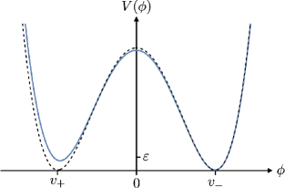
Figure 1: Schematic form of the scalar potential in (41). The dashed black curve represents the $\varepsilon=0$ case while the solid blue curve shows the $\varepsilon\neq 0$ case.

On the other hand, let us recall the conditions on the masses $m_{\pm}$ at the two vacua. For large $m_{-}$, the Casimir energy density is exponentially suppressed Anchordoqui:2023woo . This implies that the transition from AdS to dS require that the mass at the true vacuum should be approximately one order of magnitude bigger than that at the false vacuum $m_{-}/m_{+}\gg 1$. However, this contradicts the condition on the mass ratio (45) from the thin-wall approximation. We therefore conclude that quartic potentials are incompatible with the conditions for the AdS $\to$ dS transition within the thin-wall approximation.

The origin of this incompatibility is that in the thin-wall limit, the two vacua have not only equal energy but also equal mass. This motivates us to start from the potential in the thin-wall limit with equal vacuum energy but different masses at the two vacua.

4 Sixth order potential

As suggested at the end of the last section, the arguments for excluding the quartic potentials suggest that the double-well potential should have different masses already in the thin-wall limit where the two minima have the same energy. In the following we construct a set of sixth order potentials that fulfill this requirement. Let $V_{0}$ be the potential in the thin-wall limit we are going to construct.

We start from making an ansatz on the first derivative of $V_{0}$. We may reduce seven real parameters in a sixth order potential to five by using the degrees of freedom of shifting $\phi$ and adding a constant to $V_{0}$. Requiring that $V_{0}$ should have only three extrema consisting of two minima and one local maximum inbetween, we reach the following ansatz on $V_{0}^{\prime}$ with five parameters:

$$V_{0}^{\prime}(\phi)=\lambda\phi(\phi-v_{-})(\phi-v_{+})[(\phi-v)^{2}+M^{2}]\,,$$ (46)

where $M$ is a real parameter and $\lambda>0$, and we fixed the local maximum to $\phi=0$. The positive definite factor $(\phi-v)^{2}+M^{2}$ ensures that $V_{0}$ has only three extrema. The masses at the extrema are

$$m_{\pm}^{2}=V_{0}^{\prime\prime}(v_{\pm}) =\lambda v_{\pm}(v_{\pm}-v_{\mp})[(v_{\pm}-v)^{2}+M^{2}]$$ (47)

and

$$V_{0}^{\prime\prime}(0) =\lambda v_{+}v_{-}(v^{2}+M^{2})\,.$$ (48)

We require that the potential should have two minima at $\phi=v_{\pm}$ and one maximum at $\phi=0$; namely $V_{0}^{\prime\prime}(v_{\pm})>0$ and $V_{0}^{\prime\prime}(0)<0$, which gives

$$v_{+}v_{-}<0\,.$$ (49)

We assume that the extrema satisfy $v_{+}<0<v_{-}$.

Another requirement is that the two minima have the same potential energy,

$$V_{0}(v_{+})=V_{0}(v_{-})\,,$$ (50)

which is equivalent to

$$\int_{v_{+}}^{v_{-}}V_{0}^{\prime}(\phi)\ d\phi=0\,.$$ (51)

This condition fixes $M^{2}$ as a function of $v_{\pm}$ and $v$,

$$M^{2}=\frac{1}{5}\left(-5v^{2}-2v_{+}^{2}-v_{+}v_{-}-2v_{-}^{2}+2v\frac{3v_{+}^{2}+4v_{+}v_{-}+3v_{-}^{2}}{v_{+}+v_{-}}\right)\,.$$ (52)

The value $V_{0}(v_{\pm})$ at the minima can be tuned by adding a constant to the potential.

To facilitate the analysis of $M^{2}$, we parameterise $v$ as

$$v={\alpha}(v_{+}+v_{-})\,,$$ (53)

and introduce

$$r:=\frac{v_{-}}{v_{+}}<0\quad{\rm and}\quad{\beta}^{2}:=\frac{M^{2}}{v_{+}^{2}}\,,$$ (54)

so that ${\alpha},r$ and ${\beta}$ are dimensionless parameters. Substituting (53) and (54) into (52) we obtain

$$5{\beta}^{2}=-(5{\alpha}^{2}-6{\alpha}+2)r^{2}-(10{\alpha}^{2}-8{\alpha}+1)r-(5{\alpha}^{2}-6{\alpha}+2)\,.$$ (55)

Note that $5{\alpha}^{2}-6{\alpha}+2>0$ for any real ${\alpha}$. The discriminant with $r$ considered a variable reads

$$\Delta_{r}=5(4{\alpha}-3)(2{\alpha}-1)^{2}\,.$$ (56)

The positivity ${\beta}^{2}>0$ is then satisfied if

$$\alpha>\frac{3}{4}~{}~{}\text{and}~{}~{}r_{+}<r<r_{-}\,,$$ (57)

where the roots $r_{\pm}$ are defined by

$$r_{\pm}=-\frac{10{\alpha}^{2}-8{\alpha}+1\pm(2{\alpha}-1)\sqrt{5(4{\alpha}-3)}}{10{\alpha}^{2}-12{\alpha}+4}\,,$$ (58)

and are both negative for ${\alpha}>3/4$.

Since $m_{\pm}^{2}:=V_{0}^{\prime\prime}(v_{\pm})$, the mass ratio can be written as

$$\frac{m_{-}^{2}}{m_{+}^{2}}=-\frac{v_{-}}{v_{+}}\frac{(v_{-}-v)^{2}+M^{2}}{(v_{+}-v)^{2}+M^{2}}=-r\frac{[r-{\alpha}(1+r)]^{2}+{\beta}^{2}}{[1-{\alpha}(1+r)]^{2}+{\beta}^{2}}\,.$$ (59)

Note that $m_{+}^{2}=0$ for

$$({\alpha},r)=\left(2,-\frac{1}{2}\right)\,,$$ (60)

pushing $m_{-}^{2}/m_{+}^{2}\to\infty$. Note also that $(r_{-},r_{+})=(-1/2,-2)$ for ${\alpha}=2$. This indicates that $m_{-}^{2}/m_{+}^{2}\gg 1$ is attainable if ${\alpha}=2$ while perturbing $r$ around $-1/2$, i.e.,

$${\alpha}=2\,,\quad r=-\frac{1}{2}-{\delta}\,,$$ (61)

where ${\delta}$ is taken to be a positive, small parameter. Using this parametrisation, we find the following relations

$$\frac{v_{-}}{v_{+}}=-\frac{1}{2}-{\delta}+\mathcal{O}({\delta}^{2})\,,\quad v=v_{+}(1-2{\delta})+\mathcal{O}({\delta}^{2})\,,$$ (62)

$${\beta}^{2}=3{\delta}+\mathcal{O}({\delta}^{2})\,,\quad\frac{m_{-}^{2}}{m_{+}^{2}}=\frac{3}{8{\delta}}[1+\mathcal{O}({\delta})]\,,\quad m_{+}^{2}=\frac{9}{2}{\lambda}v_{+}^{4}{\delta}+\mathcal{O}({\delta}^{2})\,,$$ (63)

and

$$V_{0}^{\prime\prime}(0)=\frac{1}{2}{\lambda}v_{+}^{4}+\mathcal{O}({\delta})=-\frac{8}{27}m_{-}^{2}+\mathcal{O}({\delta})\,.$$ (64)

Under this parametrisation, the first derivative of the potential reads

$$V_{0}^{\prime}(\phi)={\lambda}\phi(\phi-v_{+})^{3}(\phi-v_{-})+\mathcal{O}({\delta})\,,$$ (65)

and so the potential is found to be

$$V_{0}(\phi)=\frac{{\lambda}}{6}(\phi-v_{+})^{4}(\phi-v_{-})^{2}+\mathcal{O}({\delta})\,,$$ (66)

where we normalised the vacuum energy to zero. Once we obtain the double-well potential $V_{0}$ in the thin-wall limit, the potential for the tunneling can be parametrised as Coleman:1977py

$$V(\phi)=V_{0}(\phi)+\varepsilon\frac{\phi-v_{-}}{v_{+}-v_{-}}\,,$$ (67)

so that the difference of the vacuum energies is still ${\varepsilon}$. A schematic representation of the potential is shown in Fig. 2.

Bearing this in mind, the difference of on-shell Euclidean actions is largely simplified and can be computed explicitly,

$$S_{1}:=\int_{v_{+}}^{v_{-}}\!\sqrt{2\left[V_{0}(\phi)-V_{0}(v_{+})\right]}\,d\phi\simeq\frac{9\sqrt{3}}{64}\sqrt{{\lambda}}v_{+}^{4}\simeq\frac{1}{4\sqrt{3{\lambda}}}m_{-}^{2}\,,$$ (68)

where we have neglected $\mathcal{O}({\delta},{\varepsilon})$. Note that $m_{-}^{2}\simeq 27{\lambda}v_{+}^{4}/16$. In closing, we note that for consistency with the form of $V(\phi)$ shown in Fig. 2, in (68) we have inverted the extrema of integration as compared to the definition of $S_{1}$ given by CdL Coleman:1980aw . Note that our choice of the extrema of integration leads to a positive $S_{1}$.

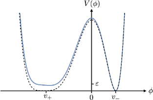
Figure 2: Schematic form of the $\phi^{6}$ scalar potential in (67). The dashed black curve represents the $\varepsilon=0$ case while the solid blue curve shows the $\varepsilon\neq 0$ case.

5 Bounce factor from dimensional analysis and lifetime prerequisite

The bounce factor of a transition from dS to Minkowski in a 5-dim spacetime with one compact dimension has been computed in Antoniadis:2024ent and is given by

$$B\simeq\frac{45\pi^{3}R_{0}S_{1}^{4}}{\varepsilon^{3}}\Bigl{[}1-\hat{\kappa}_{5}+\mathcal{O}(\hat{\kappa}_{5}^{2})\Bigr{]}\,,$$ (69)

whereas in a 5-dim spacetime with non-compact dimensions the result of CdL generalizes to

$$B\simeq\frac{2048\pi^{2}S_{1}^{5}}{15\varepsilon^{4}}\Bigl{[}1-\frac{40}{21}\hat{\kappa}_{5}+\mathcal{O}(\hat{\kappa}_{5}^{2})\Bigr{]}\,,$$ (70)

where $\hat{\kappa}_{5}:=\kappa_{5}S_{1}^{2}/{\varepsilon}$ is a dimensionless version of the five-dimensional reduced Planck length to the third power $\kappa_{5}$ introduced in Antoniadis:2024ent , controlling the gravitational correction to the bounce in the presence of gravity. Next, we consider the gravity-decoupling limit, in which only the overall coefficients matter. In the thin-wall approximation, the scalar field $\phi$ varies on the wall, while the dimensionless scale factor $\rho$ of the spherical bubble (with radius $H^{-1}$) is considered nearly constant $\bar{\rho}$. Then, the result for the compact dimension should be valid in the regime where the radius $R_{0}$ of the compact dimension is smaller than the radius $\bar{\rho}H^{-1}\simeq S_{1}/\varepsilon$ of the 3-sphere. When $R_{0}$ is larger than the latter, one should expect to reproduce the 5-dim non-compact result for the bounce, which is achieved by letting $R_{0}\simeq S_{1}/\varepsilon$. This is quantified in the negative mode analysis of the CdL instanton discussed in Sec. 2. Substituting

$$\bar{\xi}=\frac{\bar{\rho}}{\sqrt{2}H}\qquad\text{and}\qquad\bar{\rho}=\frac{9\sqrt{2}HS_{1}}{3\varepsilon+2\kappa_{5}S_{1}^{2}}\,\,,$$ (71)

into (39) it is straightforward to see that in the limit $\kappa_{5}\rightarrow 0$ the compactification radius is constrained to satisfy

$$\bar{\xi}=\frac{3S_{1}}{\varepsilon}\qquad\Rightarrow\qquad R_{0}<\frac{\sqrt{3}S_{1}}{\varepsilon}\,\,.$$ (72)

Putting all this together, the bounce configuration can be classified according to its two regimes:

• $O(4)\times U(1)$ symmetric bounce in ${\mathbf{R}}^{4}\times S^{1}/\mathbf{Z}_{2}$, for which $R_{0}<\sqrt{3}\ S_{1}/\varepsilon$;

• $O(5)$ symmetric bounce in ${\mathbf{R}}^{5}$, for which $R_{0}>\sqrt{3}\ S_{1}/\varepsilon$.

In the following, we will use a unifying symbol $D$, which actually has already appeared in Eq. (8): $D=4$ for the regime with the $O(4)\times U(1)$ symmetric bounce in ${\mathbf{R}}^{4}\times S^{1}/\mathbf{Z}_{2}$, and $D=5$ for the second regime with $O(5)$ symmetric bounce in ${\mathbf{R}}^{5}$. Note that $D$ is equal to the number of moduli of the bounce in each case. See Section 2.

The 5-dim action at the classical bounce on ${\mathbf{R}}^{4}\times S^{1}/\mathbf{Z}_{2}$ is found to satisfy

$$\text{$O(4)\times U(1)$ symmetric regime}: \quad R_{0}<\frac{\sqrt{3}\ S_{1}}{\varepsilon},\quad B\simeq\frac{1400}{2}\frac{R_{0}S_{1}^{4}}{\varepsilon^{3}},$$ (73)

$$\text{$O(5)$ symmetric regime}: \quad R_{0}>\frac{\sqrt{3}\ S_{1}}{\varepsilon},\quad B\simeq\frac{1350}{2}\frac{S_{1}^{5}}{\varepsilon^{4}},$$ (74)

where the factor of two in the denominator in both cases comes from the orbifold $S^{1}/\mathbf{Z}_{2}$ describing a line interval with two ends.

In anticipation to our calculations we recall that the AdS $\to$ dS transition at $z_{c}$ demands the lifetime of the meta-stable vacuum to be about half the age of the universe, i.e.,

$$\tau\sim 3.3\times 10^{32}~{}{\rm eV}^{-1}\,.$$ (75)

In addition, we require the mass ratio $m_{-}/m_{+}$ and the vacuum energy difference ${\varepsilon}$ of our sixth order potential $V$ to satisfy Anchordoqui:2023woo

$$\frac{m_{-}}{m_{+}}\gtrsim 5$$ (76)

and

$${\varepsilon}\ll\Lambda_{5}\sim(20\,\mbox{meV})^{5}\,.$$ (77)

Now, (76) yields ${\delta}\lesssim 0.01$ (see Eq. (63)). The lifetime of the false vacuum is related to the decay rate (8) by

$$\tau\sim\left(\frac{{\Gamma}}{V_{D-1}}\right)^{-1/D}\,.$$ (78)

The relation (78) can be rewritten as

$$B\sim D\ln\left(\tau A^{1/D}\right)\,.$$ (79)

To proceed further, we need a more explicit expression of the one-loop factor $A$, which is defined by Callan:1977pt

$$A=\left(\frac{B}{2\pi}\right)^{D/2}\left|\frac{\det^{\prime}O_{\text{B}}}{\det O_{\text{FV}}}\right|^{-1/2},$$ (80)

where the factor $(B/(2\pi))^{D/2}$ comes from the integration measure on the moduli space. $O_{\text{B}}$ and $O_{\text{FV}}$ are the differential operators that define the eigenmode equations for linear fluctuations around the bounce $\phi_{\mathrm{B}}$ and the false vacuum $v_{+}$, respectively, (see also Sec. 2)

$$O_{\text{B}} =-\triangle_{d}+V^{\prime\prime}(\phi_{\mathrm{B}})\,,$$ (81)

$$O_{\text{FV}} =-\triangle_{d}+V^{\prime\prime}(v_{+})\,.$$ (82)

The primed determinant $\det^{\prime}O_{\text{B}}$ is the determinant of $O_{\text{B}}$ with four zero modes with spin 1 removed, and $\det O_{\text{FV}}$ is the full determinant of $O_{\text{FV}}$. Each zero mode of $O_{\mathrm{B}}$ corresponds to each modulus of the bounce and hence the number of the zero modes is $D$. Since $O_{\mathrm{B}}$ and $O_{\mathrm{FV}}$ have mass dimension 2, the ratio ${\det^{\prime}O_{\text{B}}}/{\det O_{\text{FV}}}$ has dimension $-2D$ and hence $A$ has dimension $D$. See Appendix A.1 for more details.

In the following, instead of using an analytic expression of $A$, we exploit the scaling factor of $A$ that carries the mass dimension $D$. We can show (see Appendix A.2) that the scale of the determinant ratio is carried by $(\sqrt{{\lambda}}v_{+}^{2})^{D}$, which is proportional to $m_{-}^{D}$ by (64). Therefore, we can express $A$ as

$$A\sim\left(\frac{B}{2\pi}\right)^{D/2}\ a\ m_{-}^{D}\,,$$ (83)

where $a$ is the dimensionless factor (note that $B$ is dimensionless). We may then rewrite Eq. (79) into a transcendental equation of $B$,

$$B\sim\frac{D}{2}\ln\frac{B}{2\pi}+D\ln(\tau\ m_{-}\ a)\,.$$ (84)

A remark is in order. Though $m_{-}$ was chosen to carry the dimension of $A$, it is possible that other parameters of dimension 1 such as $m_{+}$ carry part or all of the mass dimension, and also that some power of $\delta$ may enter $A$ as an overall factor. Such ambiguity amounts to the ambiguity about $a$.

Though concrete expression and numerical value of $a$ are difficult to obtain, we can actually demonstrate that this does not contribute a big factor, thus not invalidating our discussion in the rest, as we will see later on. For the meantime, we will just set $a=1$ for simplicity. Using our fiducial value $m_{-}\sim 500~{}\text{meV}$, we can solve the equation (84) numerically to obtain

$$\text{$O(4)\times U(1)$ symmetric regime}: \quad B\sim 304\,,$$ (85)

and

$$\text{$O(5)$ symmetric regime}: \quad B\sim 380\,.$$ (86)

Next, we investigate the consequences of (85) and (86) by combining them with the expressions of $B$ given in (73) and (74) to obtain

$$\text{$O(4)\times U(1)$ symmetric regime}: \quad\frac{S_{1}}{\varepsilon}\sim\left(\frac{300}{700}\frac{1}{R_{0}\varepsilon}\right)^{1/4},$$ (87)

and

$$\text{$O(5)$ symmetric regime}: \quad\frac{S_{1}}{\varepsilon}\sim\left(\frac{380}{675}\frac{1}{\varepsilon}\right)^{1/5}.$$ (88)

For concreteness, we assume $R_{0}\sim 10\,\mu\text{m}\sim 50\,\text{eV}^{-1}$ and $\varepsilon\lesssim(2\,\mbox{meV})^{5}$, yielding

$$R_{0}\varepsilon\lesssim 10^{-12}\,\text{eV}^{4}.$$ (89)

Combining (89) with the expression of $S_{1}/\varepsilon$ in (87) and (88), we estimate a bound on $S_{1}/\varepsilon$ for both regimes:

• For the $O(5)$ symmetric regime, we obtain

  $$\frac{S_{1}}{\varepsilon}\sim\left(\frac{380}{675}\frac{1}{\varepsilon}\right)^{1/5}\gtrsim 445\,\text{eV}^{-1},$$ (90)

  which is incompatible with the definition of the 5-dim non-compact configuration of the bound,

  $$\frac{S_{1}}{\varepsilon}<\frac{R_{0}}{\sqrt{3}}\sim 29~{}\text{eV}^{-1}.$$ (91)

• For the $O(4)\times U(1)$ symmetric regime, we obtain

  $$\frac{S_{1}}{\varepsilon}\sim\left(\frac{300}{700}\frac{1}{R_{0}\varepsilon}\right)^{1/4}\gtrsim 720\,\text{eV}^{-1},$$ (92)

  which turns out to automatically satisfy the stability condition,

  $$\frac{S_{1}}{\varepsilon}>\frac{R_{0}}{\sqrt{3}}\sim 29~{}\text{eV}^{-1}.$$ (93)

  Here we come back to the effect of the parameter $a$ in Eq. (84). As $a$ increases, the solution $B$ increases. Concretely, as $a$ varies from $10^{-4}$ to $10^{4}$, the solution $B$ varies from 260 to 340 for the $O(4)\times U(1)$ symmetric bounce ($D=4$). In accord, the value of $S_{1}/{\varepsilon}$ varies from 700 to 740, still satisfying the stability condition. $S_{1}/{\varepsilon}$ saturates the stability condition when $a$ goes down to order $\mathcal{O}(10^{-31})$.

All in all, a 5-dim instanton with a compact dimension can naturally explain an AdS $\to$ dS transition at $z\sim 2$.

Decoupling limit of gravity

Let us justify our assumption of neglecting the gravitational corrections, namely $\hat{\kappa}_{5}\sim 0$. We consider the regime with the $O(4)\times U(1)$ symmetric bounce. The first relation in (92) can be rewritten as

$$\frac{S_{1}^{2}}{{\varepsilon}}\sim\left(\frac{3{\varepsilon}}{7R_{0}}\right)^{1/2}\,.$$ (94)

The gravitational correction becomes important when $\hat{\kappa}_{5}\gtrsim 1$, which is equivalent to

$$M_{*}^{3}\lesssim\frac{S_{1}^{2}}{{\varepsilon}}\sim\left(\frac{3{\varepsilon}}{7R_{0}}\right)^{1/2}\,,$$ (95)

where $M_{*}$ is the species scale (see Sec. 1), related to $\kappa_{5}$ as $\kappa_{5}=M_{*}^{-3}$, and we used (94) in the second step. This can be further rewritten in terms of the ratio of the vacuum energy scale ${\varepsilon}^{1/5}$ to the Planck mass $M_{*}$,

$$\frac{{\varepsilon}^{1/5}}{M_{*}}\gtrsim\left(\frac{7}{3}R_{0}M_{*}\right)^{1/5}\sim 10^{4}\,,$$ (96)

where we used $R_{0}\sim 50\,\text{eV}$ and $M_{*}\sim 10^{9}\,\text{GeV}$. However, this big lower bound means the breakdown of the effective theoretical treatment of our 5-dim action of $\phi$, and it is also impossible in the context of our analysis due to the upper bound on ${\varepsilon}$ given by (77).

6 Conclusions

We have particularised the analysis of vacuum decay in the presence of a compact dimension presented elsewhere Antoniadis:2024ent to validate the hypotheses of an AdS $\to$ dS transition driven by the Casimir forces of fields inhabiting the incredible bulk of the dark dimension scenario. Such a transition was proposed in Anchordoqui:2023woo to explain a late time ($z\sim 2$) rapid sign-switching cosmological constant, which can significantly improved the fit to observational data and resolves the $H_{0}$ and $S_{8}$ tensions Akarsu:2023mfb .

We adopted the Callan-Coleman-de Luccia formalism for calculating the transition probability within the thin-wall approximation. We have shown that the Euclidean bounce configuration that drives the vacuum decay cannot be realised by a quartic potential and we have used a minimal sixth order one. We have also shown that distinctive features of the required vacuum decay to accommodate the AdS $\to$ dS transition are inconsistent with a 5-dim non-compact description of the instanton, for which the bounce is $O(5)$ symmetric, and instead call for 5-dim instanton with a compact dimension, for which the bounce is $O(4)\times U(1)$ symmetric.

We end by noting that the Dark Energy Spectroscopic Instrument (DESI) Collaboration recently measured a tight relation between $H_{0}$ and the distance to the Coma cluster Said:2024pwm . More recently, it was noted that the inverse distance ladder of the Hubble diagram from the DESI relation combined with $H_{0}$ as determined by CMB observations with $\Lambda$CDM extrapolation leads to an Earth-Coma distance $d_{\rm EC}=(111.8\pm 1.8)~{}{\rm Mpc}$, which is $4.6\sigma$ larger than the value $d_{\rm EC}=(98.5\pm 2.2)~{}{\rm Mpc}$ obtained from calibrating the absolute magnitude of SNe Ia with the Hubble Space Telescope distance ladder Scolnic:2024hbh . Needless to say, the canonical value $95\lesssim d_{\rm EC}/{\rm Mpc}\lesssim 100$ is consistent with the $H_{0}$ measurement by SH0ES  Riess:2021jrx ; Murakami:2023xuy . It is hard to imagine how Coma could be located as far as $>110~{}{\rm Mpc}$. By extending the Hubble diagram to Coma, DESI data point to a momentous conflict between our knowledge of local distances and cosmological expectations from $\Lambda$CDM extrapolations. A late time rapid sign-switching cosmological constant based on the ideas discussed in this paper would provide a resolution of the Earth-Coma-distance conflict.

Appendix A One-loop determinant ratio

In this Appendix, we give some properties of the determinants of differential operators we used in the main part and describe how the scale of the one-loop determinant ratio is determined.

A.1 Determinants

We first summarise definitions and properties of the determinants. We recall the definitions:

$$O_{\text{B}} =-\triangle_{d}+V^{\prime\prime}(\phi_{\mathrm{B}})\,,$$ (97)

$$O_{\text{FV}} =-\triangle_{d}+V^{\prime\prime}(v_{+})\,.$$ (98)

We follow the notations given in Sec. 2.

A.1.1 $O(d)$ symmetric bounce

In this case, the determinant $\det O_{\mathrm{B}}$ is given by

$$\det O_{\mathrm{B}}=\prod_{\ell\geq 0}(\det\tilde{O}_{{\mathrm{B}},\ell})^{\mathfrak{d}_{\ell,d}}\,,\qquad\det\tilde{O}_{{\mathrm{B}},\ell}=\prod_{h_{\ell}\in{\sigma}(\tilde{O}_{{\mathrm{B}},\ell})}h_{\ell}\,,$$ (99)

where the power $\mathfrak{d}_{\ell,d}$ reflects the multiplicity of each eigenvalue of $\tilde{O}_{{\mathrm{B}},\ell}$.

Since $\tilde{O}_{{\mathrm{B}},1}$ has one zero eigenvalue, the spin-1 part $\det\tilde{O}_{{\mathrm{B}},1}$ becomes zero. We therefore modify this into $\det{}^{\prime}\tilde{O}_{{\mathrm{B}},1}$ by removing the zero mode,

$$\det{}^{\prime}\tilde{O}_{{\mathrm{B}},\ell}:=\prod_{\begin{subarray}{c}h_{\ell}\in{\sigma}(\tilde{O}_{{\mathrm{B}},\ell})\\ h_{\ell}\neq 0\end{subarray}}h_{\ell}\,.$$ (100)

The total determinant after this replacement is denoted with prime by

$$\det{}^{\prime}O_{\mathrm{B}}:=\det\tilde{O}_{{\mathrm{B}},0}\cdot(\det{}^{\prime}\tilde{O}_{{\mathrm{B}},1})^{d}\prod_{\ell=2}^{\infty}(\det\tilde{O}_{{\mathrm{B}},\ell})^{\mathfrak{d}_{\ell,d}}\,.$$ (101)

We also need $\det O_{\mathrm{FV}}$ since the decay rate is expressed with the determinant ratio as (80) Callan:1977pt . The corresponding radial differential operator $\tilde{O}_{\mathrm{FV},\ell}$ in the spin $\ell$ representation of $O(d)$ is obtained by replacing $V^{\prime\prime}(\phi_{\mathrm{B}})$ in $\tilde{O}_{{\mathrm{B}},\ell}$ (20) by $V^{\prime\prime}(v_{+})=m_{+}^{2}$. The determinant $\det O_{\mathrm{FV}}$ is defined in the same way,

$$\det O_{\mathrm{FV}}=\prod_{\ell\geq 0}(\det\tilde{O}_{\mathrm{FV},\ell})^{\mathfrak{d}_{\ell,d}}\,,\qquad\det\tilde{O}_{\mathrm{FV},\ell}=\prod_{h_{\ell}\in{\sigma}(\tilde{O}_{\mathrm{FV},\ell})}h_{\ell}\,,$$ (102)

where ${\sigma}(\tilde{O}_{\mathrm{FV},\ell})$ is the set of all eigenvalues of $\tilde{O}_{\mathrm{FV},\ell}$. The determinant ratio then reads

$$\frac{\det{}^{\prime}O_{\mathrm{B}}}{\det O_{\mathrm{FV}}}=\frac{\det\tilde{O}_{{\mathrm{B}},0}}{\det\tilde{O}_{\mathrm{FV},0}}\left[\frac{\det{}^{\prime}\tilde{O}_{{\mathrm{B}},1}}{\det\tilde{O}_{\mathrm{FV},1}}\right]^{d}\prod_{\ell=2}^{\infty}\left[\frac{\det\tilde{O}_{{\mathrm{B}},\ell}}{\det\tilde{O}_{\mathrm{FV},\ell}}\right]^{\mathfrak{d}_{\ell,d}}\,,$$ (103)

which makes sense because $\tilde{O}_{\mathrm{FV},\ell}$ is positive definite for any $\ell$. Since $\det{}^{\prime}\tilde{O}_{{\mathrm{B}},1}$ is missing one eigenvalue and the other determinant ratios $(\ell\neq 1)$ are dimensionless, the total ratio $\det{}^{\prime}O_{\mathrm{B}}/\det O_{\mathrm{FV}}$ has mass dimension $-2d$.

A remark is that $\tilde{O}_{\mathrm{FV},0}$ might seem to have eigenvalue $m_{+}^{2}$ with a non-vanishing, constant eigenfunction, but it is not true because this eigenfunction contradicts the boundary condition in (19).

A.1.2 $O(d-1)\times U(1)$ symmetric bounce

In this case, the determinant is given by

$$\det O_{\mathrm{B}}=\prod_{\ell=0}^{\infty}~{}(\widehat{\det}\,\tilde{O}_{{\mathrm{B}},\ell})^{\mathfrak{d}_{\ell,d-1}}\,,$$ (104)

$$\widehat{\det}\,\tilde{O}_{{\mathrm{B}},\ell}:=\prod_{h_{\ell}\in{\sigma}_{\mathrm{KK}}(\tilde{O}_{{\mathrm{B}},\ell})}~{}\prod_{s=0}^{\infty}\left(h_{\ell}+\frac{s^{2}}{R_{0}^{2}}\right)\,.$$ (105)

Since $\tilde{O}_{{\mathrm{B}},1}$ has one zero eigenvalue, the spin-1 part $\widehat{\det}\,\tilde{O}_{{\mathrm{B}},1}$ is zero. We therefore modify this into $\widehat{\det}{}^{\prime}\,\tilde{O}_{{\mathrm{B}},1}$ by removing the zero mode,

$$\widehat{\det}{}^{\prime}\,\tilde{O}_{{\mathrm{B}},\ell}=\prod_{\begin{subarray}{c}h_{\ell}\in{\sigma}_{\mathrm{KK}}(\tilde{O}_{{\mathrm{B}},\ell})\\ h_{\ell}\neq 0\end{subarray}}~{}\prod_{s=0}^{\infty}\left(h_{\ell}+\frac{s^{2}}{R_{0}^{2}}\right)\,.$$ (106)

The total determinant under this replacement is given with prime by

$$\det{}^{\prime}O_{\mathrm{B}}=\widehat{\det}\,\tilde{O}_{{\mathrm{B}},0}\cdot(\widehat{\det}{}^{\prime}\,\tilde{O}_{{\mathrm{B}},1})^{d-1}\prod_{\ell=2}^{\infty}~{}\widehat{\det}\,\tilde{O}_{{\mathrm{B}},\ell}\,.$$ (107)

Let us next consider $\det O_{\mathrm{FV}}$. The corresponding radial differential operator $\tilde{O}_{\mathrm{FV},\ell}$ in the spin $\ell$ representation of $O(d-1)$ is obtained by replacing $V^{\prime\prime}(\phi_{\mathrm{B}})$ in $\tilde{O}_{{\mathrm{B}},\ell}$ (33) by $V^{\prime\prime}(v_{+})=m_{+}^{2}$. The determinant $\det O_{\mathrm{FV}}$ is defined in the same way,

$$\det O_{\mathrm{FV}}=\prod_{\ell=0}^{\infty}~{}(\widehat{\det}\,\tilde{O}_{\mathrm{FV},\ell})^{\mathfrak{d}_{\ell,d-1}}\,,$$ (108)

$$\widehat{\det}\,\tilde{O}_{\mathrm{FV},\ell}:=\prod_{h_{\ell}\in{\sigma}(\tilde{O}_{\mathrm{FV},\ell})}~{}\prod_{s=0}^{\infty}\left(h_{\ell}+\frac{s^{2}}{R_{0}^{2}}\right)\,,$$ (109)

where ${\sigma}(\tilde{O}_{\mathrm{FV},\ell})$ is the set of all eigenvalues of $\tilde{O}_{\mathrm{FV},\ell}$. The determinant ratio then reads

$$\frac{\det{}^{\prime}O_{\mathrm{B}}}{\det O_{\mathrm{FV}}}=\frac{\widehat{\det}\,\tilde{O}_{{\mathrm{B}},0}}{\widehat{\det}\,\tilde{O}_{\mathrm{FV},0}}\left[\frac{\widehat{\det}{}^{\prime}\,\tilde{O}_{{\mathrm{B}},1}}{\widehat{\det}\,\tilde{O}_{\mathrm{FV},1}}\right]^{d-1}\prod_{\ell=2}^{\infty}\left[\frac{\widehat{\det}\,\tilde{O}_{{\mathrm{B}},\ell}}{\widehat{\det}\,\tilde{O}_{\mathrm{FV},\ell}}\right]^{\mathfrak{d}_{\ell,d-1}}\,,$$ (110)

which makes sense because $\tilde{O}_{\mathrm{FV},\ell}$ is positive definite for any $\ell$. Since $\widehat{\det}{}^{\prime}\,\tilde{O}_{{\mathrm{B}},1}$ is missing one eigenvalue and the other determinant ratios $(\ell\neq 1)$ are dimensionless, the total ratio $\det{}^{\prime}\,O_{\mathrm{B}}/\det O_{\mathrm{FV}}$ has mass dimension $-2(d-1)$.

As in the $O(d)$ symmetric case, $m_{+}^{2}$ is not an eigenvalue of $\tilde{O}_{\mathrm{FV},0}$ because its nonvanishing, constant eigenfunction contradicts the boundary condition in (32).

A.2 Scaling behaviour

We start from the EoM for the bounce, which reads

$$\ddot{\phi}_{\mathrm{B}}(\xi)+\frac{D-1}{\xi}\dot{\phi}_{\mathrm{B}}(\xi)-V^{\prime}(\phi_{\mathrm{B}})=0\,,$$ (111)

where $V(\phi)$ is the sixth order potential (67), and $D=4$ for the $O(4)\times U(1)$ symmetric bounce in ${\mathbf{R}}^{4}\times S^{1}/\mathbf{Z}_{2}$ and $D=5$ for the $O(5)$ symmetric bounce in ${\mathbf{R}}^{5}$. Let us rescale the radial coordinate $\xi$, the parameter ${\varepsilon}$, and the bounce $\phi_{\mathrm{B}}$ to make them dimensionless,

$$z=\sqrt{{\lambda}}v_{+}^{2}\xi\,,\quad{\varphi}_{\mathrm{B}}(z):=\frac{\phi_{\mathrm{B}}(\xi)}{v_{+}}\,,\quad\hat{\varepsilon}:=\frac{{\varepsilon}}{{\lambda}v_{+}^{6}}\,.$$ (112)

In terms of the dimensionless quantities, the EoM becomes

$$\frac{d^{2}{\varphi}_{\mathrm{B}}}{dz^{2}}+\frac{3}{z}\frac{d{\varphi}_{\mathrm{B}}}{dz}=\hat{V}^{\prime}_{0}({\varphi}_{\mathrm{B}})+\frac{\hat{\varepsilon}}{1-r}\,,$$ (113)

where $\hat{V}^{\prime}_{0}({\varphi}_{\mathrm{B}})={\varphi}_{\mathrm{B}}({\varphi}_{\mathrm{B}}-1)({\varphi}_{\mathrm{B}}-r)^{3}$. Since this EoM contains only dimensionless parameters $r$ and $\hat{\varepsilon}$, the parameters in the dimensionless bounce ${\varphi}_{\mathrm{B}}$ are only $r$ and $\hat{\varepsilon}$.

Let us rescale the eigenmode equation $O_{\mathrm{B}}\eta=h\eta$ around the $O(4)\times U(1)$ symmetric bounce with (112) together with $\hat{y}=\sqrt{{\lambda}}v_{+}^{2}y$. The result is

$$\left[-\frac{\partial^{2}}{\partial z^{2}}-\frac{3}{z}\frac{\partial}{\partial z}-\frac{\triangle_{S^{d-2}}}{z^{2}}+\hat{V}^{\prime\prime}({\varphi}_{\mathrm{B}})+\frac{{\partial}^{2}}{{\partial}\hat{y}^{2}}\right]\eta=\frac{h}{{\lambda}v_{+}^{4}}\eta\,.$$ (114)

Since the parameters on its left hand side are only $r,\hat{\varepsilon}$, the eigenvalue $h/({\lambda}v_{+}^{4})$ is a dimensionless quantity with these parameters. Therefore, the dimension of eigenvalue $h$ is carried by ${\lambda}v_{+}^{4}$, which is proportional to $m_{-}^{2}$ by (62). Concretely, each eigenvalue can be expressed as (see also Sec. 2.2)

$$m_{-}^{2}\left(\frac{h_{\ell}}{m_{-}^{2}}+\frac{s^{2}}{m_{-}^{2}R_{0}^{2}}\right)\,,$$ (115)

where the term with the round bracket is dimensionless and $h_{\ell}/m_{-}^{2}$ is a function of $r$ and $\hat{\varepsilon}$. This argument goes in a parallel manner in the case of the $O(5)$ symmetric bounce. It is also obvious that the same argument holds for $O_{\mathrm{FV}}\eta=h\eta$ around the false vacuum. Therefore, in both cases, any eigenvalue of the eigenmode equations can be written as a product of the factor $m_{-}^{2}$ and a dimensionless quantity depending on $r,\hat{\varepsilon}$ and $m_{-}R_{0}$.

Therefore, the mass dimension $-2D$ of the determinant ratio $\det{}^{\prime}\,O_{\mathrm{B}}/\det O_{\mathrm{FV}}$, where $D$ is the number of the moduli of the bounce solution, is carried by the factor $m_{-}^{-2D}$, and hence the one-loop factor $A$ in (80) can be expressed as (83),

$$A\sim\left(\frac{B}{2\pi}\right)^{D/2}\ a\ m_{-}^{D}\,,$$ (116)

where $a$ is a function of dimensionless quantities $r,\hat{\varepsilon}$ and $m_{-}R_{0}$. Note that $A$ should exist in the limit $r\to-1/2$ $({\delta}\to 0)$ and $\hat{\varepsilon}\to 0$.

A remark is in order. The rescaling (112) is not the unique one, but we may further multiply powers of dimensionless factors. For example, we can adopt the rescaling so that the dimension 2 of the eigenvalues is carried by $m_{+}^{2}$ instead of $m_{-}^{2}$. For the one-loop factor $A$, this change of the scale factor can be absorbed into the change in the dependence of the dimensionless parameter $a$ on the mass ratio $m_{+}^{2}/m_{-}^{2}\sim{\delta}$.

References

- (1) Particle Data Group Collaboration, S. Navas et al., “Review of Particle Physics,” Phys. Rev. D 110 (2024) 030001.
- (2) E. Abdalla et al., “Cosmology intertwined: A review of the particle physics, astrophysics, and cosmology associated with the cosmological tensions and anomalies,” JHEAp 34 (2022) 49–211, arXiv:2203.06142 [astro-ph.CO].
- (3) Planck Collaboration, N. Aghanim et al., “Planck 2018 results. VI. Cosmological parameters,” Astron. Astrophys. 641 (2020) A6, arXiv:1807.06209 [astro-ph.CO]. [Erratum: Astron.Astrophys. 652, C4 (2021)].
- (4) D. Scolnic et al., “The Pantheon+ Analysis: The Full Data Set and Light-curve Release,” Astrophys. J. 938 no. 2, (2022) 113, arXiv:2112.03863 [astro-ph.CO].
- (5) A. G. Riess et al., “A Comprehensive Measurement of the Local Value of the Hubble Constant with 1 km s-1 Mpc-1 Uncertainty from the Hubble Space Telescope and the SH0ES Team,” Astrophys. J. Lett. 934 no. 1, (2022) L7, arXiv:2112.04510 [astro-ph.CO].
- (6) Y. S. Murakami, A. G. Riess, B. E. Stahl, W. D. Kenworthy, D.-M. A. Pluck, A. Macoretta, D. Brout, D. O. Jones, D. M. Scolnic, and A. V. Filippenko, “Leveraging SN Ia spectroscopic similarity to improve the measurement of H 0,” JCAP 11 (2023) 046, arXiv:2306.00070 [astro-ph.CO].
- (7) C. Heymans et al., “KiDS-1000 Cosmology: Multi-probe weak gravitational lensing and spectroscopic galaxy clustering constraints,” Astron. Astrophys. 646 (2021) A140, arXiv:2007.15632 [astro-ph.CO].
- (8) E. Di Valentino, O. Mena, S. Pan, L. Visinelli, W. Yang, A. Melchiorri, D. F. Mota, A. G. Riess, and J. Silk, “In the realm of the Hubble tension—a review of solutions,” Class. Quant. Grav. 38 no. 15, (2021) 153001, arXiv:2103.01183 [astro-ph.CO].
- (9) N. Schöneberg, G. Franco Abellán, A. Pérez Sánchez, S. J. Witte, V. Poulin, and J. Lesgourgues, “The H0 Olympics: A fair ranking of proposed models,” Phys. Rept. 984 (2022) 1–55, arXiv:2107.10291 [astro-ph.CO].
- (10) L. Perivolaropoulos and F. Skara, “Challenges for CDM: An update,” New Astron. Rev. 95 (2022) 101659, arXiv:2105.05208 [astro-ph.CO].
- (11) O. Akarsu, J. D. Barrow, L. A. Escamilla, and J. A. Vazquez, “Graduated dark energy: Observational hints of a spontaneous sign switch in the cosmological constant,” Phys. Rev. D 101 no. 6, (2020) 063528, arXiv:1912.08751 [astro-ph.CO].
- (12) O. Akarsu, S. Kumar, E. Özülker, and J. A. Vazquez, “Relaxing cosmological tensions with a sign switching cosmological constant,” Phys. Rev. D 104 no. 12, (2021) 123512, arXiv:2108.09239 [astro-ph.CO].
- (13) O. Akarsu, S. Kumar, E. Özülker, J. A. Vazquez, and A. Yadav, “Relaxing cosmological tensions with a sign switching cosmological constant: Improved results with Planck, BAO, and Pantheon data,” Phys. Rev. D 108 no. 2, (2023) 023513, arXiv:2211.05742 [astro-ph.CO].
- (14) O. Akarsu, E. Di Valentino, S. Kumar, R. C. Nunes, J. A. Vazquez, and A. Yadav, “CDM model: A promising scenario for alleviation of cosmological tensions,” arXiv:2307.10899 [astro-ph.CO].
- (15) S. A. Adil, U. Mukhopadhyay, A. A. Sen, and S. Vagnozzi, “Dark energy in light of the early JWST observations: case for a negative cosmological constant?,” JCAP 10 (2023) 072, arXiv:2307.12763 [astro-ph.CO].
- (16) N. Menci, S. A. Adil, U. Mukhopadhyay, A. A. Sen, and S. Vagnozzi, “Negative cosmological constant in the dark energy sector: tests from JWST photometric and spectroscopic observations of high-redshift galaxies,” JCAP 07 (2024) 072, arXiv:2401.12659 [astro-ph.CO].
- (17) A. Bernui, E. Di Valentino, W. Giarè, S. Kumar, and R. C. Nunes, “Exploring the H0 tension and the evidence for dark sector interactions from 2D BAO measurements,” Phys. Rev. D 107 no. 10, (2023) 103531, arXiv:2301.06097 [astro-ph.CO].
- (18) A. Gómez-Valent, A. Favale, M. Migliaccio, and A. A. Sen, “Late-time phenomenology required to solve the H0 tension in view of the cosmic ladders and the anisotropic and angular BAO datasets,” Phys. Rev. D 109 no. 2, (2024) 023525, arXiv:2309.07795 [astro-ph.CO].
- (19) J. D. Barrow, “Sudden future singularities,” Class. Quant. Grav. 21 (2004) L79–L82, arXiv:gr-qc/0403084.
- (20) E. A. Paraskevas, A. Cam, L. Perivolaropoulos, and O. Akarsu, “Transition dynamics in the sCDM model: Implications for bound cosmic structures,” Phys. Rev. D 109 no. 10, (2024) 103522, arXiv:2402.05908 [astro-ph.CO].
- (21) D. Lüst, E. Palti, and C. Vafa, “AdS and the Swampland,” Phys. Lett. B 797 (2019) 134867, arXiv:1906.05225 [hep-th].
- (22) L. A. Anchordoqui, I. Antoniadis, and D. Lüst, “Anti-de Sitter → de Sitter transition driven by Casimir forces and mitigating tensions in cosmological parameters,” Phys. Lett. B 855 (2024) 138775, arXiv:2312.12352 [hep-th].
- (23) O. Akarsu, A. De Felice, E. Di Valentino, S. Kumar, R. C. Nunes, E. Ozulker, J. A. Vazquez, and A. Yadav, “CDM cosmology from a type-II minimally modified gravity,” arXiv:2402.07716 [astro-ph.CO].
- (24) O. Akarsu, A. De Felice, E. Di Valentino, S. Kumar, R. C. Nunes, E. Ozulker, J. A. Vazquez, and A. Yadav, “Cosmological constraints on CDM scenario in a type II minimally modified gravity,” arXiv:2406.07526 [astro-ph.CO].
- (25) M. Montero, C. Vafa, and I. Valenzuela, “The dark dimension and the Swampland,” JHEP 02 (2023) 022, arXiv:2205.12293 [hep-th].
- (26) I. Antoniadis, N. Arkani-Hamed, S. Dimopoulos, and G. R. Dvali, “New dimensions at a millimeter to a Fermi and superstrings at a TeV,” Phys. Lett. B 436 (1998) 257–263, arXiv:hep-ph/9804398.
- (27) L. A. Anchordoqui and I. Antoniadis, “Large extra dimensions from higher-dimensional inflation,” Phys. Rev. D 109 no. 10, (2024) 103508, arXiv:2310.20282 [hep-ph].
- (28) N. Arkani-Hamed, S. Dubovsky, A. Nicolis, and G. Villadoro, “Quantum Horizons of the Standard Model Landscape,” JHEP 06 (2007) 078, arXiv:hep-th/0703067.
- (29) I. Antoniadis, D. Bielli, A. Chatrabhuti, and H. Isono, “Thin-wall vacuum decay in the presence of a compact dimension,” JHEP 09 (2024) 011, arXiv:2405.16920 [hep-th].
- (30) S. R. Coleman and F. De Luccia, “Gravitational Effects on and of Vacuum Decay,” Phys. Rev. D 21 (1980) 3305.
- (31) C. G. Callan, Jr. and S. R. Coleman, “The Fate of the False Vacuum. 2. First Quantum Corrections,” Phys. Rev. D 16 (1977) 1762–1768.
- (32) L. A. Anchordoqui, I. Antoniadis, D. Lüst, N. T. Noble, and J. F. Soriano, “From infinite to infinitesimal: Using the Universe as a dataset to probe Casimir corrections to the vacuum energy from fields inhabiting the dark dimension,” arXiv:2404.17334 [astro-ph.CO].
- (33) A. Yadav, S. Kumar, C. Kibris, and O. Akarsu, “CDM cosmology: Alleviating major cosmological tensions by predicting standard neutrino properties,” arXiv:2406.18496 [astro-ph.CO].
- (34) S. R. Coleman, “The Fate of the False Vacuum. 1. Semiclassical Theory,” Phys. Rev. D 15 (1977) 2929–2936. [Erratum: Phys.Rev.D 16, 1248 (1977)].
- (35) H. Lee and E. J. Weinberg, “Negative modes of Coleman-De Luccia bounces,” Phys. Rev. D 90 no. 12, (2014) 124002, arXiv:1408.6547 [hep-th].
- (36) H. Isono, T. Noumi, and G. Shiu, “Momentum space approach to crossing symmetric CFT correlators. Part II. General spacetime dimension,” JHEP 10 (2019) 183, arXiv:1908.04572 [hep-th].
- (37) K. Said et al., “DESI Peculiar Velocity Survey – Fundamental Plane,” arXiv:2408.13842 [astro-ph.CO].
- (38) D. Scolnic et al., “The Hubble Tension in our own Backyard: DESI and the Nearness of the Coma Cluster,” arXiv:2409.14546 [astro-ph.CO].