PASTRAMI: Performance Assessment of SofTware Routers Addressing Measurement Instability

Abstract

Virtualized environments offer a flexible and scalable platform for evaluating network performance, but they can introduce significant variability that complicates accurate measurement. This paper presents PASTRAMI, a methodology designed to assess the stability of software routers, which is critical to accurately evaluate performance metrics such as the Partial Drop Rate at 0.5% (PDR@0.5%). While PDR@0.5% is a key metric to assess packet processing capabilities of a software router, its reliable evaluation depends on consistent router performance with minimal measurement variability. Our research reveals that different Linux versions exhibit distinct behaviors, with some demonstrating non-negligible packet loss even at low loads and high variability in loss measurements, rendering them unsuitable for accurate performance assessments. This paper proposes a systematic approach to differentiate between stable and unstable environments, offering practical guidance on selecting suitable configurations for robust networking performance evaluations in virtualized environments.

I Introduction

Virtualized architectures can be a valuable tool to characterize modern cloud-based infrastructures. In many scenarios, complex and expensive hardware and software devices are used to evaluate network performance. These devices, although very high-performance, are very often unsuitable because their physical nature makes them not very suitable to dynamic deployment in a datacenter infrastructure. However, with the evolution of networking and the AI, it is necessary to move a large amount of data with good resilience. Typically, with the concentration of resources in large datacenters, data is mostly confined to these structures. It has therefore become necessary to test these infrastructures dynamically to avoid and prevent malfunctions and loss of services. In this area, software solutions can play a crucial role due to their versatility. It is possible to perform performance tests using simple COTS servers available anywhere in the datacenter. Many current software solutions can generate a large amount of packets to send through the network. At the same time, they can receive the return packets and monitor performance metrics. These software can run on bare metal servers and can perform measurements directly on production hardware. A very important aspect currently in use is the migration from the traditional approach of providing services on a single server to a virtualized environment where a single hardware resource can host a multiplicity of services. Therefore, thanks to this approach it has been possible to multiply the flexibility and availability of resources by exploiting the available hardware more efficiently. Virtualization is a technology that allows multiple virtual instances of computing resources—such as servers, storage devices, networks, or operating systems—to be created and managed on a single physical hardware system. This abstraction enables efficient utilization of resources, isolation, and flexibility in deploying and managing applications. A looser approach is containerization. Containerization is a technology that allows for the packaging of an application and its dependencies into a single, standardized unit called a container. This container can run consistently across different computing environments, such as development, testing, and production. Both techniques can be combined with each other by expanding the capabilities and resources available on a single hardware server. Another advantage brought by virtualization is the decoupling between software and hardware resources, allowing flexibility and resilience and scalability of services within the infrastructure in a dynamic way. In this particular context, networks have also had their important evolution. We have moved from physical networking that interconnects the various physical devices such as servers, switches and routers to virtual networking that dynamically interconnects virtual resources and services through virtual switches and virtual routers as well as interfacing with physical networking when it is necessary to go out to the virtual environment. Virtual networking has become crucial in this area and measuring its performances allows to improve its changes considering the high resources and stringent requirements required by big data flows. Virtualized environments offer a powerful means of assessing network performance, providing unique benefits and flexibility that traditional setups cannot match. They enable organizations to efficiently test various network configurations, model different traffic scenarios, and ultimately improve the performance and stability of their networks. However, to maximize the effectiveness of such environments, consideration must be given to the inherent challenges and limitations associated with virtualization, ensuring that assessments are both accurate and meaningful.

II Background and Related Work

• Overview of PDR@0.5% and its relevance in evaluating packet processing capabilities.

• Explanation of PDR@0.5% as a performance evaluation metric.

The Partial Drop Rate (PDR) at 0.5% (PDR@0.5%) metric, as described in [1], provides a way to assess the performance of a system under test (SUT) by identifying the highest input rate that allows for a Delivery Ratio (DR) of at least 99.5%. DR is defined as the ratio between the output and input packet rates of the SUT. This metric, along with the No-Drop Rate (NDR), offers a useful tool to compare performance across different devices or configurations. While NDR represents the maximum rate without any packet loss, PDR@X% incorporates an acceptable packet loss threshold, making PDR@0.5% a more realistic measure for systems that may experience small packet losses due for example to limitations in CPU or NIC interrupt handling.

By reducing the entire load-performance relationship to a single scalar value, PDR@0.5% simplifies performance evaluation. This makes it easier to quantitatively compare various systems, configurations, or software implementations, without needing to analyze the full throughput curve. The typical example along this line is to use PDR@0.5% to evaluate the performance of different variants or versions of packet processing functions in software routers, or the performance cost of introducing additional functionality in the packet processing operations.

However, while the PDR@0.5% metric provides a convenient summary of performance, its usage may need to be limited to stable environments where consistent performance can be ensured. One critical issue is that reducing complex performance behavior to a single scalar value can obscure important nuances in the system’s response to varying loads. In other words, the metric does not capture information about the system’s performance at lower loads or higher loads. This is particularly problematic in environments where performance may fluctuate due to factors like CPU contention, interrupt handling, or network stack inefficiencies, as PDR@0.5% assumes a stable environment. By focusing on a single point (0.5% loss), this metric inherently overlooks fluctuations in throughput or other instability issues that may emerge at other points along the load-loss curve. Consequently, PDR@0.5% should be applied with caution, particularly in environments prone to variability, and supplemented with additional metrics to ensure a more comprehensive evaluation of performance.

Another limitation of using PDR@0.5% exclusively is that it assumes the system operates stably up to that point, ignoring any variability in performance. In practice, however, many systems exhibit performance fluctuations under certain conditions, especially in virtualized environments, where factors like CPU contention or network stack inefficiencies can lead to inconsistent results. These issues are not captured by PDR@0.5%, which may result in overly optimistic conclusions about a system’s robustness.

Moreover, PDR@0.5% may not adequately reflect the system behavior for higher loads, where congestion control mechanisms, buffer management, and other factors become significant. In these cases, understanding how a system behaves at higher packet loss rates or under full saturation would provide a more comprehensive view of its capabilities. Therefore, while PDR@0.5% is useful for providing a high-level comparison, it should be supplemented with additional analysis of the system behavior across a broader range of operating conditions to ensure a more complete performance evaluation.

• Review of challenges in using virtualized environments for network performance evaluation, including variability issues.

Virtualized environments are a common choice for evaluating network capabilities and performance. They are flexible, scalable, and cost-effective. However, they also present challenges that can affect the accuracy and reliability of network performance measurements. The two most important challenges to consider when using virtual environments for performance assessment are: i) variability and ii) the overhead associated with virtualization. A virtualized environment is dynamic, with flexible resource allocation and deallocation. Variations in the allocation of CPU, memory, bandwidth, and settings to virtual environments can negatively affect performance evaluation. In addition, because virtual environments share the same hardware, they can interfere with each other and compete for the same resources. On the other hand, virtualized environments are complex and often computationally expensive. The virtualization layer may introduce an overhead that can affect network performance, making it challenging to isolate and measure the performance of individual components.

• Summary of previous work on network measurement instability and virtualization effects.

III Methodological aspects

III-A Reference configurations

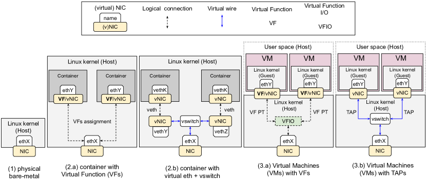
Figure 1: Reference configurations

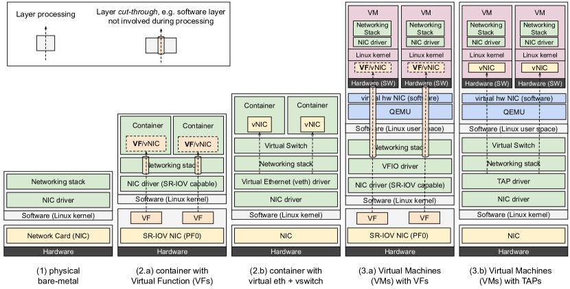
Figure 2: Layer impacting performance in different example configurations

AM: Da qui inizia la descrizione delle figure 1 e 2

Fig. 1 illustrates the different types of virtualization environments that should be considered when measuring network performance. Considering Fig. 1-(1), the virtualization environment is very basic, as it uses only the networking capabilities provided by the Linux kernel that runs natively on the hardware. In this case, the Linux environment is used without any kind of network virtualization.

Referring to Fig. 1-(2.a), the virtualization environment is based on Linux Containers. This technology allows applications and services to run in an environment isolated from the Host operating system, while still sharing resources such as memory, CPU, etc. In Fig. 1-(2.a), however, Containers use dedicated virtual NICs to communicate with each other and the outside world. Such virtual NICs are called Virtual Functions (VFs). By using VFs, a physical network adapter (supporting SR-IOV[2]) can be partitioned into multiple virtual adapters. Each virtual adapter can operate independently and it appears to the Host as a physical network card, with its own PCI address. Virtualization in this configuration adds minimal overhead as shown in Fig. 2-(2.a). Packet processing is primarily carried out by the network card driver, which supports SR-IOV and the Linux networking capabilities within the Container.

In consideration of the topology depicted in Fig. 1-(2.b), the virtualization environment relies on Virtual Ethernet Pairs (veths) to facilitate communication between the Host and Containers. In Linux, a veth is defined as a pair of virtual Ethernet devices (endpoints) that are connected to each other. Packets are sent to one endpoint and received by the other. A veth pair functions like an Ethernet cable, enabling communication between network namespaces, e.g. foundation block of the Linux Containers.

Virtual Ethernet pairs are entirely software-based, so there is no need for costly hardware-enabled Virtual Functions to connect the Host and Containers. Fig. 2-(2.b) indicates that additional packet processing is needed to exchange packets between the Host and Containers. The Virtual Ethernet driver manages these interfaces and handles packets sending/receiving operations. A software-based virtual switch is needed to connect Containers to the Host network, increasing the overall processing overhead.

Fig. 1-(3.a) illustrates an alternative virtual environment topology using Virtual Machines (VMs) instead of Linux Containers. A VM is typically implemented on Linux using QEMU/KVM, [3] [4] a robust virtualization solution that enables users to run multiple isolated operating systems (Guests) on a single machine. QEMU/KVM provides virtual hardware to Guests, including CPUs, memory management, and I/O virtualization. VMs running on Linux execute as processes and cannot directly interact with the Host hardware. VM access to Host hardware, including the NICs, is enabled by device pass-through. Fig. 1.(3.a) shows how Virtual Function I/O (VFIO) [5] kernel driver allows a VM access hardware directly. In this scenario, the Host is equipped with a SR-IOV-capable NIC and the VFIO driver is used to make VFs available to the Guests. Fig. 2-(3.a) reveals that when VFs are passed through to VMs, the overall overhead is reduced to bare minimum as the VMs can directly access the NIC hardware resources of the Host.

When VFs or SR-IOV NICs are unavailable on the Host, VMs can use virtual NICs, as shown in Fig. 1-(3.b). QEMU can emulate multiple network cards, which Guests see as hardware NICs (e.g. PCI cards). Guest NICs can be connected to the Host network through a variety of mechanisms, frequently involving the use of virtual Host Ethernet devices (TAPs) [6], as reported in Fig. 2-(3.b). The TAP device bridges the VM and Host network, enabling VM packet transmission and reception. Fully software-emulated NIC solutions may have performance issues. QEMU provides optimisation techniques (whenever possible), including VirtIO [7] and paravirtualization, to reduce packet processing overhead and facilitate communication between the Guest and the Host.

III-B Definition of metrics for load-loss analysis

• Coarse load/loss analysis: loss and standard deviation of loss in each load condition

We define the offered load $O$ [p/s] as the rate of packets that are sent to an incoming interface of the system under test (SUT). For simplicity, we now assume that all packets have the same size at the IP layer $S$ [Bytes]. We also assume that the offered load is constant over time in our observation interval of duration $T$: $O(t)=O$ for each $t\in T$.

Let us now count the number $N$ of packets that are correctly forwarded by the SUT in the interval $T$. The average throughput of the SUT over $T$ is $R(O)=\frac{N}{T}$ [p/s], where $R(O)\leq O$.

We can count the number of Lost Packets $L$ over the interval $T$ as $L=(O\cdot T)-N$ (all packets that have NOT arrived are lost!). We define the Packet Loss Ratio (PLR) of the SUT for an offered load $O$ over an observation interval $T$ as:

$$PLR(O)=\frac{L}{O\cdot T}$$

The PLR can also be expressed as follows:

$$PLR(O)=\frac{O\cdot T-N}{O\cdot T}=1-\frac{N}{O\cdot T}=1-\frac{R(O)}{O}$$

We define the Delivery Ratio $DR$ as $DR(O)=\frac{R(O)}{O}$, then we can express the packet loss ratio as a function of the Delivery Ratio:

$$PLR(O)=1-DR(O)$$

In the above discussion, we simply assumed that we can count the number $N$ of packets forwarded with an experiment of duration $T$. In the real world, when we perform a number of $K$ repetitions of an experiment (each with duration $T$) with the same offered load $O$, we will have in general $K$ different values of $N$ and therefore of $L$: $L(O,i)$ for $i\in[0,K-1]$. For this reason, we resort to a statistical characterization of our metrics $PLR(O)$, $T(O)$, and $DR(O)$.

We define $PLR(O)$ as:

$$PLR(O)=\frac{1}{K}\sum_{i=0}^{K-1}\frac{L(O,i)}{O\cdot T}$$

The standard deviation of the measurements, denoted as $\sigma_{\text{PLR}}(O)$, based on a population sample is given by:

$$\sigma_{\text{PLR}}(O)=\sqrt{\frac{1}{K-1}\sum_{i=0}^{K-1}\left(\frac{L(O,i)}{O\cdot T}-PLR(O)\right)^{2}}$$ (1)

We are interested in evaluating the reliability of our estimated metric $PLR(O)$ (the same reasoning can be applied to $T(O)$, and $DR(O)$). In particular, we consider the confidence interval at 95%, defined as:

$$P(\text{LCL}_{95}<PLR(O)<\text{UCL}_{95})=0.95$$

where $\text{LCL}_{95}$ and $\text{UCL}_{95}$ are the lower and upper confidence limits for a 95% confidence interval, respectively.

When the standard deviation of the population $\sigma$ is unknown and estimated using the sample standard deviation $\sigma_{\text{PLR}}(O)$ from $K$ independent observations, the 95% confidence interval for the true parameter $PLR(O)$ is given by:

$$PLR(O)\pm t_{K-1,\,0.025}\cdot\frac{\sigma_{\text{PLR}}(O)}{\sqrt{K}}$$

where:

• $t_{K-1,\,0.025}$ is the critical value from the Student’s t-distribution with $K-1$ degrees of freedom (97.5th percentile, reflecting the 95% confidence level),

• $\sigma_{\text{PLR}}(O)$ is the standard deviation, calculated as in Eq. 1,

• $K$ is the number of experiments.

The use of the $t$-distribution accounts for the additional uncertainty due to estimating the variance from a sample rather than knowing it exactly.

The lower and upper confidence limits can be computed separately as follows:

$$\text{LCL}_{95}=PLR(O)-t_{K-1,\,0.025}\cdot\frac{\sigma_{\text{PLR}}(O)}{\sqrt{K}}$$

$$\text{UCL}_{95}=PLR(O)+t_{K-1,\,0.025}\cdot\frac{\sigma_{\text{PLR}}(O)}{\sqrt{K}}$$

The $\text{LCL}_{95}$ represents the lower bound of the 95% confidence interval, indicating the smallest value that the true $PLR(O)$ is likely to be with 95% confidence. Similarly, the $\text{UCL}_{95}$ represents the upper bound of the 95% confidence interval, indicating the largest value that the true $PLR(O)$ is likely to be with 95% confidence.

To further evaluate the uncertainty of our estimate $PLR(O)$, we introduce a normalized metric that considers the upper bound of the 95% confidence interval. The normalized metric, $\Delta_{\text{UCL}_{95}}$, is defined as:

$$\Delta_{\text{UCL}_{95}}=\frac{\text{UCL}_{95}-PLR(O)}{PLR(O)}$$

The metric $\Delta_{\text{UCL}_{95}}$ provides a dimensionless measure of the relative uncertainty in the estimate of $PLR(O)$. A smaller value of $\Delta_{\text{UCL}_{95}}$ indicates that the upper confidence limit is close to $PLR(O)$, suggesting higher precision in the estimate. In contrast, a larger value indicates that there is a greater uncertainty in the estimation relative to its magnitude.

III-C Ideal vs. real load-loss curves

Let us define the concepts of saturation throughput and ideal load-loss curve. The saturation throughput, denoted as $T^{\text{sat}}$, is the maximum throughput that a system can sustain before packet losses increase significantly. It is reached when the offered load $O$ equals the saturation offered load $O^{\text{sat}}$. For loads beyond this point, the throughput remains constant:

$$T(O)=T^{\text{sat}},\quad O\geq O^{\text{sat}}$$

where $T^{\text{sat}}=O^{\text{sat}}\cdot(1-PLR(O^{\text{sat}}))$. In an ideal system, the load-loss curve starts with a packet loss ratio (PLR) of 0, which persists for all offered loads up to the saturation point $O^{\text{sat}}$. For loads greater than $O^{\text{sat}}$, the PLR increases according to Eq. 2 (see Fig. 3).

$$PLR(O)=\frac{O-T^{\text{sat}}}{O}=1-\frac{T^{\text{sat}}}{O}$$ (2)

In a realistic system, the packet loss starts at 0, then it initially remains on the order of $10^{-8}$ to $10^{-6}$, and then smoothly increases up to a loss ratio of $10^{-2}$ (i.e., 1% loss) This behavior arises due to factors such as the interrupt-driven packet processing, limited buffering capacity, or other inefficiencies in the packet forwarding mechanisms. These small losses occur even at relatively low loads, before the system reaches $O^{\text{sat}}$.

When the offered load exceeds $O^{\text{sat}}$, the throughput in a realistic system may begin to decline, rather than staying constant as in the ideal case. This can be described by the following function:

$$T(O)=f(O-O^{\text{sat}})\cdot T^{\text{sat}},\quad O>O^{\text{sat}}$$ (3)

where $f(0)=1$, $f(x)>0$, and $f(x)$ is a non-increasing function.

For example, we can identify a threshold $O^{\text{trash}}$ for the offered load, such that the system goes into trashing and decreases its throughput with increasing offered load. Just as an example, this can be expressed by defining a stepwise linear $f(x)$ to be used in Eq. 3 as follows:

$$f(x)=\begin{cases}1&O^{\text{sat}}<x<O^{\text{trash}},\\ \max\left(0,1-\frac{x-O^{\text{trash}}}{M}\right)&x\geq O^{\text{trash}}\end{cases}$$ (4)

where $M>0\quad[Mpps]$ is a positive constant with dimension mega packets/s. This adjustment reflects that, in real-world conditions, factors such as congestion, buffer overflow, or resource limitations can cause the throughput to decrease when the load exceeds the saturation threshold.

To sum up, a realistic load-loss curve is characterized by non-zero PLR values before $O^{\text{sat}}$, by a non-zero $PLR(O^{\text{sat}})$ and by a declining throughput when the offered load exceeds the saturation point. Fig. 4 represents a more realistic synthetic loss curve generated using Eq. 3 and Eq. 4.

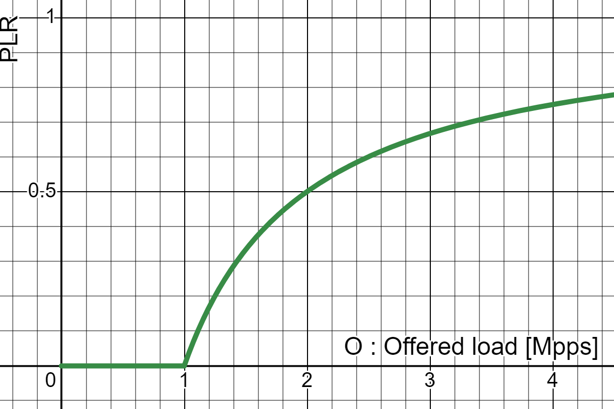
Figure 3: Ideal load-loss curve, where the saturation offered load is 1 Mpps and the saturation throughput equals the saturation offered load.

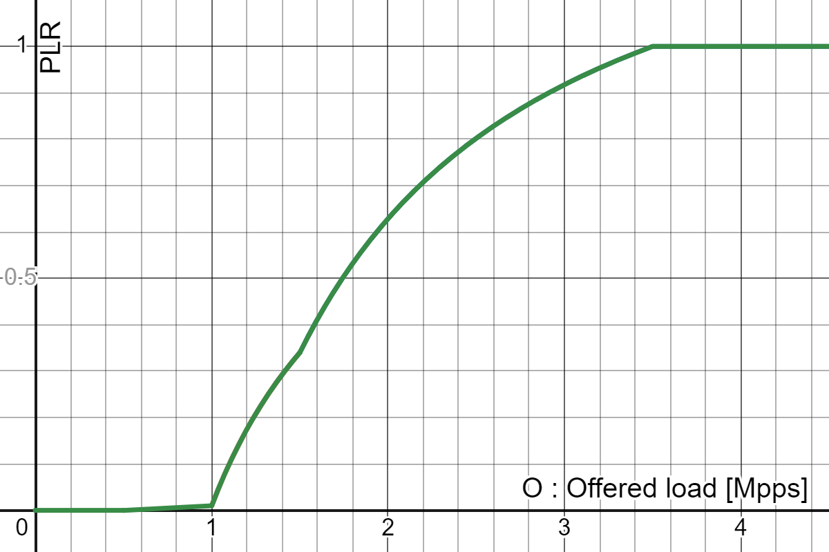
Figure 4: A more realistic synthetic load-loss curve, where the saturation offered load is 1 Mpps, the saturation throughput equals 0.99 of the saturation offered load (PLR at saturation is 1%), the trashing threshold $O^{\text{trash}}$ is 1.5 Mpps and $M$ is 1 Mpps.

Plotting the load-loss curve in linear scale as in Figs. 3 and 4 does not provide useful information for the region of low offered load/low loss represented on the left part of the figure. For this reason, we can use a logarithmic scale to represent the loss ratio on the y axis. On such a scale, it is not possible to represent a zero loss ratio which would correspond to minus infinite, and we have to arbitrarily choose a packet loss ratio at the bottom of the scale. We chose $10^{-6}$ because it corresponds to a value of the packet loss ratio that is not even possible to be evaluated reliably with measurement sessions of reasonable duration. In Fig. 5 we plot both the ideal and the realistic loss ratio curves in log scale. It is clear how we can easily differentiate the performance for the offered load below 1 Mpps between the ideal and the realistic loss-load curves, which on the other hand are barely indistinguishable in Figs. 3 and 4

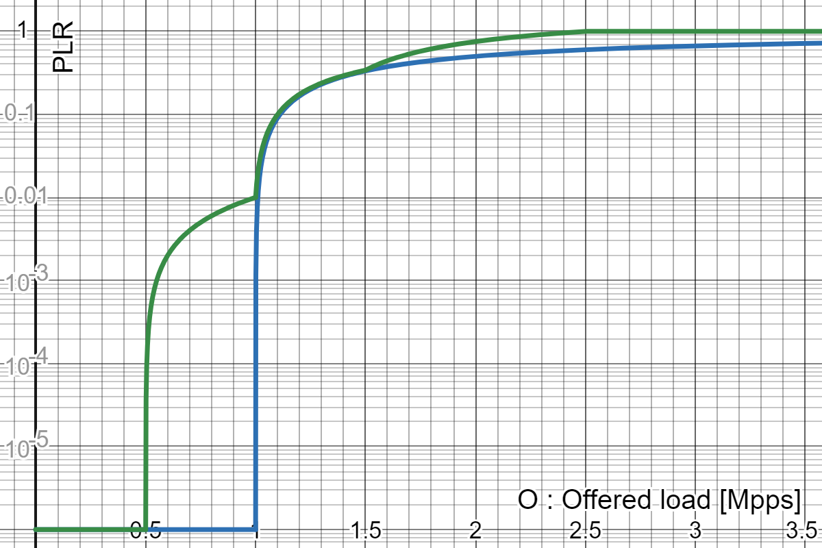
Figure 5: Both the ideal (blue) and the more realistic (green) load-loss curves are plotted in log scale, considering as the bottom of scale a loss ratio of $10^{-6}$.

• Description of experimental setup: bare metal vs virtualized environments, router configurations, and Linux versions used, cloudlab vs local measurement environment

III-D Considerations about stability analysis

• Importance of stability in measurements: how instability can distort performance metrics.

SS: TO BE SHORTENED AM: ho provato a riassumere

In order to assess complex systems, measurements must be taken in a controlled manner to check whether such systems satisfy the desired requirements. To obtain accurate performance data, measurements must be stable. Any form of instability can lead to the collection of invalid data, which can then influence decisions and lead to invalid conclusions. Therefore, measurement stability is important for consistency and repeatability. Most critically, instability makes it impossible to identify trends or patterns in the data when analyzing experiments designed to determine the systems and/or components performance. Inaccurate measurements lead to flawed decisions.

SS: END TO BE SHORTENED

Analysis of the loss ratio and standard deviation of the loss ratio under different load conditions is one way to quantify the measurement instability. Loss ratio analysis compares the actual performance of a system/component with the expected performance under a predetermined and controlled environment. Instead, the standard deviation of the loss ratio provides a quantitative measure of how much the measured performance deviates from the expected level of performance. A high standard deviation of the loss ratio indicates that there is significant variability in the results, suggesting measurement instability.

III-E Experimental space

The space of the experiments is defined by various aspects that can be modified to explore different configurations. These aspects include:

• Number of Runs: The number of repetitions for a single measurement. The default is 50 runs, but this can be varied.

• Duration of a Single Experiment: The duration for each experiment, which by default is set to 10 seconds.

• Environment: Experiments can be performed on bare metal servers or within virtualized environments.

• Linux Kernel Versions: Different kernel versions are tested to observe their impact on performance. The available versions are:

  • 5.15

  • 6.5

  • 6.8

• CPU Pinning: Various CPU pinning strategies are applied for managing the RX and TX tasks:

  • unpinned: No specific CPU pinning is applied.

  • pin-1-cpu: All RX and TX processing tasks are pinned to a single CPU.

  • pin-2-cpu: RX processing tasks are pinned to one CPU, and TX processing tasks are pinned to a second CPU.

• NIC Ring Buffer Size: The size of the NIC ring buffer can be adjusted as follows:

  • SMALL-nic-buf: Default buffer size of 512 packets.

  • LARGE-nic-buf: Increased buffer size of 4096 packets.

The complete list of configuration options is summarized in Table I.

Aspect	Options
Number of Runs	50 (default), configurable
Duration (seconds)	10 (default), configurable
Environment	• Bare metal server • Virtualized environment
Linux Kernel Versions	• 5.15 • 6.5 • 6.8
CPU Pinning	• unpinned • pin-1-cpu (RX and TX tasks on 1 CPU) • pin-2-cpu (RX on 1 CPU, TX on 2nd CPU)
NIC Ring Buffer Size	• SMALL-nic-buf (512 packets) • LARGE-nic-buf (4096 packets)

TABLE I: Configuration options for the experimental space.

IV Evaluation of load/loss curve over bare metal software routers

• Coarse load/loss analysis of out-of-the-box Linux on bare metal (cloudlab) infrastructure

• Linux OK (6.8) vs Linux KO (5.15)

• (nice to have) host same switch vs remote hosts

• Coarse load/loss analysis of out-of-the-box Linux on virtualized infrastructure (cloudlab)

• Linux OK vs Linux KO

V Description of experimental setup

• Description of experimental setup: Virtualized environments, router configurations, and Linux versions used.

VI Results and Analysis

• Comparison of performance across different Linux versions.

• Cases of instability: high variability and non-negligible packet loss at low loads.

• Analysis of the effects of instability on the accuracy of PDR@0.5% evaluation.

VII Discussion

• Implications of instability for networking research in virtualized environments.

• Potential causes of instability: OS versions, virtualization layers, kernel interactions.

• Recommended practices to reduce instability and improve measurement reliability.

VIII Proposed Methodology for Stability Assessment

• Detailed methodology to assess the stability of network routers.

• Steps for applying the PASTRAMI approach to ensure consistent measurement conditions.

• Recommendations for practitioners on how to choose and configure environments to minimize variability.

IX Conclusion and Future Work

• Summary of findings: stability as a prerequisite for accurate performance evaluation using PDR@0.5%.

• Future directions: automation of stability checks, investigation of other virtualization platforms, or deeper exploration of variability sources.

References

- [1] A. Abdelsalam, P. L. Ventre, C. Scarpitta, A. Mayer, S. Salsano, P. Camarillo, F. Clad, and C. Filsfils, “SRPerf: a Performance Evaluation Framework for IPv6 Segment Routing,” IEEE Transactions on Network and Service Management, vol. 18, no. 2, pp. 2320–2333, 2020.
- [2] “Single Root I/O Virtualization (SR-IOV).” [Online]. Available: https://docs.kernel.org/PCI/pci-iov-howto.html
- [3] Qemu - a generic and open source machine emulator and virtualizer. [Online]. Available: https://www.qemu.org/
- [4] Kernel virtual machine. [Online]. Available: https://www.linux-kvm.org/
- [5] “VFIO - “Virtual Function I/O”.” [Online]. Available: https://docs.kernel.org/driver-api/vfio.html
- [6] “Universal TUN/TAP device driver.” [Online]. Available: https://www.kernel.org/doc/Documentation/networking/tuntap.txt
- [7] “Virtual I/O Device (VIRTIO).” [Online]. Available: https://docs.oasis-open.org/virtio/virtio/v1.2/virtio-v1.2.html