Diffusion Attribution Score:
Evaluating Training Data Influence in Diffusion Model

Abstract

As diffusion models become increasingly popular, the misuse of copyrighted and private images has emerged as a major concern. One promising solution to mitigate this issue is identifying the contribution of specific training samples in generative models, a process known as data attribution. Existing data attribution methods for diffusion models typically quantify the contribution of a training sample by evaluating the change in diffusion loss when the sample is included or excluded from the training process. However, we argue that the direct usage of diffusion loss cannot represent such a contribution accurately due to the calculation of diffusion loss. Specifically, these approaches measure the divergence between predicted and ground truth distributions, which leads to an indirect comparison between the predicted distributions and cannot represent the variances between model behaviors. To address these issues, we aim to measure the direct comparison between predicted distributions with an attribution score to analyse the training sample importance, which is achieved by Diffusion Attribution Score (DAS). Underpinned by rigorous theoretical analysis, we elucidate the effectiveness of DAS. Additionally, we explore strategies to accelerate DAS calculations, facilitating its application to large-scale diffusion models. Our extensive experiments across various datasets and diffusion models demonstrate that DAS significantly surpasses previous benchmarks in terms of the linear data-modelling score, establishing new state-of-the-art performance.

1 Introduction

Diffusion models, highlighted in key studies (Ho et al., 2020; Song et al., 2021b), are advancing significantly in generative machine learning with broad applications from image generation to artistic creation (Saharia et al., 2022; Hertz et al., 2023; Li et al., 2022; Ho et al., 2022). As these models, exemplified by projects like Stable Diffusion (Rombach et al., 2022), become increasingly capable of producing high-quality, varied outputs, the misuse of copyrighted and private images has become a significant concern. A key strategy to address this issue is identifying the contributions of training samples in generative models by evaluating their influence on the generated images, a task known as data attribution. Data attribution in machine learning is essential for tracing model outputs back to influential training examples and understanding how specific data points affect model behavior. In practical applications, data attribution spans various domains, including explaining predictions (Koh & Liang, 2017; Yeh et al., 2018; Ilyas et al., 2022), curating datasets (Khanna et al., 2019; Jia et al., 2021; Liu et al., 2021), and dissecting the mechanisms of generative models like GANs and VAEs (Kong & Chaudhuri, 2021; Terashita et al., 2021), serving to enhance model transparency and explore the effect of training data on model behaviors.

Data attribution methods generally fall into two categories. The first, based on sampling (Shapley et al., 1953; Ghorbani & Zou, 2019; Ilyas et al., 2022), involves retraining models to assess how outputs change with the deletion of specific data. While effective, this method requires training thousands of models—a formidable challenge given today’s large-scale models. The second approach uses approximations to assess the change in output for efficiency (Koh & Liang, 2017; Feldman & Zhang, 2020; Pruthi et al., 2020), which may compromise precision. Recent advancements have led to innovative estimators like TRAK (Park et al., 2023), which linearizes model behavior using a kernel matrix analogous to the Fisher Information Matrix. Additionally, Zheng et al. (2024) proposed D-TRAK, which adapts TRAK to diffusion models by setting the output function as the diffusion loss. However, this setting conducts an indirect comparison between the predicted distributions since the diffusion loss is equivalent to the divergence between predicted and ground truth distributions (Ho et al., 2020). They also reported counterintuitive findings that the diffusion loss can be replaced with other output functions without modifying the form of the attribution score, and the results of these empirical designs surpass diffusion loss with theoretical designs, highlighting the need for a deeper understanding of diffusion models in data attribution.

In this paper, we first present a theoretical analysis to address the challenges associated with directly applying TRAK to diffusion models, which also explain the counter-intuitive observations noted in D-TRAK. Further, we propose a novel attribution method termed Diffusion Attribution Score (DAS), specifically designed for diffusion models to quantitatively assess the impact of training samples on model outputs by measuring the divergence between predicted distributions when the sample is included or excluded from the training set, which includes a self-contained derivation. Additionally, we explore several techniques to expedite the computation of DAS, such as compressing models or datasets, enabling its application to large-scale diffusion models and significantly enhancing the practicability of our approach. The primary contributions of our work are summarized as follows:

1. We offer a comprehensive analysis of the limitations when directly applying TRAK to diffusion tasks. This theoretical examination sheds light on the empirical success of D-TRAK and fosters the development of more effective attribution methods.

2. We introduce DAS, a theoretically solid metric designed to directly quantify discrepancies in model outputs, supported by detailed derivations. We also discuss various techniques, such as compressing models or datasets, to accelerate the computation of DAS, facilitating its efficient implementation.

3. DAS demonstrates state-of-the-art performance across multiple benchmarks, notably excelling in linear datamodeling scores.

2 Preliminaries

2.1 Diffusion Models

Our study concentrates on discrete-time diffusion models, specifically Denoising Diffusion Probabilistic Models (DDPMs) (Ho et al., 2020) and Latent Diffusion Models (LDMs) which are foundational to Stable Diffusion (Rombach et al., 2022). This paper grounds all theoretical derivations related to diffusion models within the framework of unconditional generation using DDPMs. Below, we detail the notation employed in DDPMs that underpins all further theoretical discussions.

Consider a training set ${\mathbb{S}}=\{{\bm{z}}^{(1)},...,{\bm{z}}^{(n)}\}$ where each training sample ${\bm{z}}^{(i)}:=({\bm{x}}^{(i)},y^{(i)})\sim\mathcal{Z}$ is an input-label pair. Given an input data distribution $q({\bm{x}})$, DDPMs aim to model a distribution $p_{\theta}({\bm{x}})$ to approximate $q({\bm{x}})$. The learning process is divided into forward and reverse process, conducted over a series of timesteps in the latent variable space, with ${\bm{x}}_{0}$ denoting the initial image and ${\bm{x}}_{t}$ the latent variables at timestep $t\in[1,T]$. In the forward process, DDPMs sample an observation ${\bm{x}}_{0}$ from ${\mathbb{S}}$ and progressively add noise on it across $T$ timesteps: $q({\bm{x}}_{t}|{\bm{x}}_{t-1}):=\mathcal{N}({\bm{x}}_{t};\sqrt{1-\beta_{t}}{\bm{x}}_{t-1},\beta_{t}{\bm{I}})$, where $\beta_{1},...,\beta_{T}$ constitute a variance schedule. As indicated in DDPMs, the latent variable ${\bm{x}}_{t}$ can be express as a linear combination of ${\bm{x}}_{0}$:

$${\bm{x}}_{t}=\sqrt{\bar{\alpha}_{t}}{\bm{x}}_{0}+\sqrt{1-\bar{\alpha}_{t}}{\bm{\epsilon}}\text{,}$$ (1)

where $\alpha_{t}:=1-\beta_{t},\bar{\alpha}_{t}:=\prod_{s=1}^{t}\alpha_{s}$ and ${\bm{\epsilon}}\sim\mathcal{N}(0,{\bm{I}})$. In the reward process, DDPMs model a distribution $p_{\theta}({\bm{x}}_{t-1}|{\bm{x}}_{t})$ by minimizing the KL-divergence from $q({\bm{x}}_{t-1}|{\bm{x}}_{t},{\bm{x}}_{0})$ at each timestep $t$:

$$D_{\mathrm{KL}}[p_{\theta}({\bm{x}}_{t-1}|{\bm{x}}_{t})\|q({\bm{x}}_{t-1}|{\bm{x}}_{t},{\bm{x}}_{0})]=\mathbb{E}_{{\bm{\epsilon}}\sim\mathcal{N}(0,{\bm{I}})}[\frac{\beta_{t}^{2}}{2\alpha_{t}(1-\bar{\alpha}_{t})}||{\bm{\epsilon}}-{\bm{\epsilon}}_{\theta}({\bm{x}}_{t},t)||^{2}]\text{,}$$ (2)

where ${\bm{\epsilon}}_{\theta}$ is a function implemented by trainable models $\theta$ which can be seen as a noise predictor. A simplified version of objective function for a data point ${\bm{x}}$ used to train DDPMs is:

$$\mathcal{L}_{\text{Simple}}({\bm{x}},\theta)=\mathbb{E}_{{\bm{\epsilon}},t}[||{\bm{\epsilon}}_{\theta}({\bm{x}}_{t},t)-{\bm{\epsilon}}||^{2}]\text{.}$$ (3)

2.2 Data Attribution

Given a DDPM trained on dataset ${\mathbb{S}}$, our objective is to trace the influence of the training data on an output generated for a particular sample ${\bm{z}}$. This task is commonly referred to as data attribution. A common approach to data attribution involves addressing a counterfactual question: if a training sample ${\bm{z}}^{(i)}$ is removed from ${\mathbb{S}}$ and a model $\theta_{\backslash i}$ is retrained on the remaining subset ${\mathbb{S}}_{\backslash i}$, the influence of ${\bm{z}}^{(i)}$ on the sample ${\bm{z}}$ can be assessed by the change in the model output, computed as $f({\bm{z}},\theta)-f({\bm{z}},\theta_{\backslash i})$. The function $f({\bm{z}},\theta)$, which represents the model output, has a variety of choices, such as the direct output of the model or its loss function.

To circumvent the high computational costs associated with retraining models, some data attribution methods compute a scoring function $\tau({\bm{z}},{\mathbb{S}}):\mathcal{Z}\times\mathcal{Z}^{n}\rightarrow\mathbb{R}^{n}$, which assigns scores reflecting the importance of each training sample in ${\mathbb{S}}$ for the sample ${\bm{z}}$ under consideration. For clarity, $\tau({\bm{z}},{\mathbb{S}})^{(i)}$ denotes the attribution score assigned to the influence of the individual training sample ${\bm{z}}^{(i)}$ on ${\bm{z}}$.

TRAK (Park et al., 2023) stands out as a representative data attribution method designed for large-scale models focused on discriminative tasks. TRAK defines the model output function as:

$$f_{\text{TRAK}}({\bm{z}},\theta)=\log[\hat{p}({\bm{x}},\theta)/(1-\hat{p}({\bm{x}},\theta))]\text{,}$$ (4)

where $\hat{p}({\bm{x}},\theta)$ represents the probability of the corresponding class $y$ for the sample ${\bm{z}}$. TRAK introduces an attribution function $\tau_{\text{TRAK}}({\bm{z}},{\mathbb{S}})^{(i)}$ designed to approximate the change in $f_{\text{TRAK}}({\bm{z}},\theta)$ following the deletion of a data point. This is expressed as:

$$\tau_{\text{TRAK}}({\bm{z}},{\mathbb{S}})^{(i)}:=\phi({\bm{z}})^{\top}({\bm{\Phi}}^{\top}{\bm{\Phi}})^{-1}\phi({\bm{z}}^{(i)})r^{(i)}\approx f_{\text{TRAK}}({\bm{z}},\theta)-f_{\text{TRAK}}({\bm{z}},\theta_{\backslash i})\text{,}$$ (5)

where $r^{(i)}=1-\hat{p}({\bm{x}}^{(i)},\theta)$ denotes the residual for sample ${\bm{z}}^{(i)}$. Here, $\phi({\bm{z}}):={\bm{P}}^{\top}\nabla_{\theta}f_{\text{TRAK}}({\bm{z}},\theta)$ and ${\bm{\Phi}}:=[\phi({\bm{z}}^{(1)}),...,\phi({\bm{z}}^{(n)})]$ represents the matrix of stacked gradients from ${\mathbb{S}}$. ${\bm{P}}\sim\mathcal{N}(0,1)^{d\times k}$ is a random projection matrix (Johnson & Lindenstrauss, 1984) employed to reduce the dimension of the gradient $\nabla_{\theta}f_{\text{TRAK}}({\bm{z}};\theta)\in\mathbb{R}^{d}$ to $k$. This function computes a score indicating the influence of a training sample ${\bm{z}}_{i}$ on the sample of interest ${\bm{z}}$ in a discriminative model setting.

To adapt TRAK in diffusion models, D-TRAK (Zheng et al., 2024) modifies the output function to align with the objective function described in Eq. 3: $f_{\text{D-TRAK}}({\bm{z}},\theta)=\mathcal{L}_{\text{Simple}}({\bm{x}},\theta)$, and simplifies the residual term to an identity matrix ${\bm{I}}$. The attribution function in D-TRAK is defined as follows:

$$\tau_{\text{D-TRAK}}({\bm{z}},{\mathbb{S}})^{(i)}=\phi({\bm{z}})^{\top}({\bm{\Phi}}^{\top}{\bm{\Phi}})^{-1}\phi({\bm{z}}^{(i)}){\bm{I}}\approx f_{\text{D-TRAK}}({\bm{z}},\theta)-f_{\text{D-TRAK}}({\bm{z}},\theta_{\backslash i})\text{,}$$ (6)

where $\phi({\bm{z}}):={\bm{P}}^{\top}\nabla_{\theta}f_{\text{D-TRAK}}({\bm{z}},\theta)$ mirrors the gradient term used in TRAK. Interestingly, D-TRAK has observed that substituting the function $f_{\text{D-TRAK}}$ with other functions can yield superior attribution performance. Examples of these include $\mathcal{L}_{\text{Square}}({\bm{z}},\theta)=\mathbb{E}_{t,{\bm{\epsilon}}}[||{\bm{\epsilon}}_{\theta}({\bm{x}}_{t},t)||^{2}]$ and $\mathcal{L}{\text{Average}}({\bm{z}},\theta)=\mathbb{E}_{t,{\bm{\epsilon}}}[\text{Avg}({\bm{\epsilon}}_{\theta}({\bm{x}}_{t},t))]$, both of which have enhanced attribution capabilities.

3 Methodology

In this section, we propose a novel data attribution method tailored for diffusion models to assess the impact of training samples on the generative process. Revisiting our objective, we aim to evaluate how training samples influence the generation within a diffusion model. Previous work D-TRAK, has applied TRAK designed for discriminative tasks to generative tasks, utilizing the Simple Loss as the output function. In Section 3.1, we critically analyze the shortcomings of employing a loss function as the output function in diffusion models and propose a more suitable output function.

Additionally, the attribution score is contingent upon the task setting and the selected output function. Alterations in the settings, such as the loss function and output function, significantly affect the derivation of the attribution score. Consequently, we introduce a new attribution metric called Diffusion Attribution Score (DAS), specifically developed for generative tasks in diffusion models, detailed in Section 3.2. In section 3.3, we explore methodologies for applying DAS to large-scale diffusion model and discuss strategies to expedite the computation process.

3.1 Rethinking the design of model output function

Reviewing the goal of data attribution within diffusion models, suppose we have a set of training data ${\mathbb{S}}$ and wish to measure the influence of a specific training sample ${\bm{z}}^{(i)}$ on a generated sample ${\bm{z}}^{\text{gen}}$. This task can be approached by addressing the counterfactual question: How would the model output change for ${\bm{z}}^{\text{gen}}$ if we removed ${\bm{z}}^{(i)}$ from ${\mathbb{S}}$ and retrained the model on the subset ${\mathbb{S}}_{\backslash i}$? D-TRAK proposes using $\tau_{\text{D-TRAK}}$ to approximate this difference based on the Simple Loss:

$$\tau_{\text{D-TRAK}}({\bm{z}}^{\text{gen}},{\mathbb{S}})^{(i)} \approx f_{\text{D-TRAK}}({\bm{z}}^{\text{gen}},\theta)-f_{\text{D-TRAK}}({\bm{z}}^{\text{gen}},\theta_{\backslash i})$$

$$=\mathbb{E}_{{\bm{\epsilon}},t}[||{\bm{\epsilon}}_{\theta}({\bm{x}}^{\text{gen}}_{t},t)-{\bm{\epsilon}}||^{2}]-\mathbb{E}_{{\bm{\epsilon}},t}[||{\bm{\epsilon}}_{\theta_{\backslash i}}({\bm{x}}^{\text{gen}}_{t},t)-{\bm{\epsilon}}||^{2}]\text{,}$$ (7)

where ${\bm{\epsilon}}_{\theta_{\backslash i}}$ denotes the noise predictor trained on ${\mathbb{S}}_{\backslash i}$. However, from a distribution perspective, this approach involves an indirect comparison of KL-divergences between the model distributions and the data distribution to indicate the distances between model distributions:

$$\tau_{\text{D-TRAK}}({\bm{z}}^{\text{gen}},{\mathbb{S}})^{(i)}\approx D_{\mathrm{KL}}[p_{\theta}({\bm{x}}^{\text{gen}})||q({\bm{x}}^{\text{gen}})]-D_{\mathrm{KL}}[p_{\theta_{\backslash i}}({\bm{x}}^{\text{gen}})\|q({\bm{x}}^{\text{gen}})]\text{.}$$ (8)

This indirect comparison may introduce errors when evaluating the differences between $p_{\theta}({\bm{x}}^{\text{gen}})$ and $p_{\theta_{\backslash i}}({\bm{x}}^{\text{gen}})$. For instance, both distributions might approach the data distribution $q({\bm{x}}^{\text{gen}})$ from different directions, yet exhibit similar distances. To enable a more direct comparison, we propose the Diffusion Attribution Score (DAS) to assess the KL-divergence between the predicted distributions:

$$\tau_{\text{DAS}}({\bm{z}}^{\text{gen}},{\mathbb{S}})^{(i)} \approx D_{\mathrm{KL}}[p_{\theta}({\bm{x}}^{\text{gen}})||p_{\theta_{\backslash i}}({\bm{x}}^{\text{gen}})]$$

$$\approx\mathbb{E}_{{\bm{\epsilon}},t}[||{\bm{\epsilon}}_{\theta}({\bm{x}}^{\text{gen}}_{t},t)-{\bm{\epsilon}}_{\theta_{\backslash i}}({\bm{x}}^{\text{gen}}_{t},t)||^{2}]\text{.}$$ (9)

The output function in DAS is defined as $f_{\text{DAS}}({\bm{z}},\theta)={\bm{\epsilon}}_{\theta}({\bm{x}}^{\text{gen}}_{t},t)$, which is able to directly reflect the differences between the noise predictors of the original and the retrained models. Eq. 9 also validates the effectiveness of employing $\mathcal{L}_{\text{square}}$ as the output function, which is formulated as:

$$\tau_{\text{Square}}({\bm{z}}^{\text{gen}},{\mathbb{S}})^{(i)}\approx\mathbb{E}_{{\bm{\epsilon}},t}[||{\bm{\epsilon}}_{\theta}({\bm{x}}^{\text{gen}}_{t},t)||^{2}]-\mathbb{E}_{{\bm{\epsilon}},t}[||{\bm{\epsilon}}_{\theta_{\backslash i}}({\bm{x}}^{\text{gen}}_{t},t)||^{2}]\text{.}$$ (10)

This approach also mitigates the influence of indirect comparisons. However, the subtraction used here does not constitute any recognized type of distance metric. Furthermore, the matrices ${\bm{\epsilon}}_{\theta}$ and ${\bm{\epsilon}}_{\theta_{\backslash i}}$ which retain the same high dimensionality as the input images ${\bm{x}}^{\text{gen}}$, should not be represented merely by scalar values, whether by average or $L^{2}$ norm, as this leads to a loss of dimensional information. For instance, these matrices might exhibit identical differences across various dimensions, an aspect that scalar representations fail to capture. This dimensional consistency is crucial for understanding the full impact of training data alterations on model outputs.

3.2 Diffusion Attribution Score

In diffusion models, the generative process involves a series of generative steps, and the model produces outputs at $T$ different timesteps. In this section, we explore methods to approximate Eq. 9 at a specific timestep $t$ without the necessity for retraining the model, which aims to evaluate the influence of training data on the model’s generation.

Linearing Output Function. Computing the output of the retrained model ${\bm{\epsilon}}_{\theta_{\backslash i}}({\bm{x}}^{\text{gen}}_{t},t)$ is computationally expensive. To enhance computational efficiency, we propose linearizing the model output function using its Taylor expansion centered around the final model parameters $\theta^{*}$, simplifying the calculation as follows:

$$f_{\text{DAS}}({\bm{z}}_{t},\theta)\approx{\bm{\epsilon}}_{\theta^{*}}({\bm{x}}_{t},t)+\nabla_{\theta}{\bm{\epsilon}}_{\theta^{*}}({\bm{x}}_{t},t)^{\top}(\theta-\theta^{*}).$$ (11)

By substituting Eq. 11 into Eq. 9, we derive:

$$\tau_{\text{DAS}}({\bm{z}}^{\text{gen}},{\mathbb{S}})^{(i)}_{t}\approx\mathbb{E}_{\bm{\epsilon}}[||\nabla_{\theta}{\bm{\epsilon}}_{\theta^{*}}({\bm{x}}_{t}^{\text{gen}},t)^{\top}(\theta^{*}-\theta^{*}_{\backslash i})||^{2}].$$ (12)

The subscript $t$ indicates the attribution score for the model output at timestep $t$. Consequently, the influence of removing a sample from subset ${\mathbb{S}}_{\backslash i}$ on the model output can now be quantitatively evaluated through the changes in model parameters, which can be measured by the leave-one-out method, thereby significantly reducing the computational overhead.

Estimating the model parameter. Consider using the leave-one-out method, the variation of the diffusion model parameters can be assessed by Newton’s Method (Pregibon, 1981). By removing a training sample ${\bm{z}}^{(i)}$, the counterfactual parameters $\theta^{*}_{\backslash i}$ can be approximated by taking a single Newton step from the optimal parameters $\theta^{*}$:

$$\theta^{*}-\theta^{*}_{\backslash i}\leftarrow-[{\nabla_{\theta}{\bm{\epsilon}}_{\theta^{*}}({{\mathbb{S}}_{\backslash i}}_{t},t)}^{\top}\nabla_{\theta}{\bm{\epsilon}}_{\theta^{*}}({{\mathbb{S}}_{\backslash i}}_{t},t)]^{-1}\nabla_{\theta}{\bm{\epsilon}}_{\theta^{*}}({\mathbb{S}}_{\backslash i},t)^{\top}{{\bm{R}}_{\backslash i}}_{t}\text{,}$$ (13)

where ${\bm{\epsilon}}_{\theta^{*}}({\mathbb{S}}_{t},t):=[{\bm{\epsilon}}_{\theta^{*}}({\bm{x}}^{(1)}_{t},t),...,{\bm{\epsilon}}_{\theta^{*}}({\bm{x}}^{(n)}_{t},t)]$ represents the stacked output matrix for the set ${\mathbb{S}}$ at timestep $t$, and ${\bm{R}}_{t}:=\text{diag}[{\bm{\epsilon}}_{\theta}({\bm{x}}^{(i)}_{t},t)-{\bm{\epsilon}}]$ is a diagonal matrix describing the residuals among ${\mathbb{S}}$. A detailed proof of Eq. 13 is provided in Appendix B.

Let ${\bm{g}}_{t}({\bm{x}}^{(i)})=\nabla_{\theta}{\bm{\epsilon}}_{\theta^{*}}({\bm{x}}^{(i)}_{t},t)$ and ${\bm{G}}_{t}({\mathbb{S}})=\nabla_{\theta}{\bm{\epsilon}}_{\theta^{*}}({\mathbb{S}}_{t},t)$. The inverse term in Eq. 13 can be reformulated as:

$${\bm{G}}_{t}({\mathbb{S}}_{\backslash i})^{\top}{\bm{G}}_{t}({\mathbb{S}}_{\backslash i})={\bm{G}}_{t}({\mathbb{S}})^{\top}{\bm{G}}_{t}({\mathbb{S}})-{\bm{g}}_{t}({\bm{x}}^{(i)})^{\top}{\bm{g}}_{t}({\bm{x}}^{(i)})\text{.}$$ (14)

Applying the Sherman–Morrison formula to Eq. 14 simplifies Eq. 13 as follows:

$$\theta^{*}-\theta^{*}_{\backslash i}\leftarrow\frac{[{\bm{G}}_{t}({\mathbb{S}})^{\top}{\bm{G}}_{t}({\mathbb{S}})]^{-1}{\bm{g}}_{t}({\bm{x}}^{(i)}){\bm{r}}^{(i)}_{t}}{1-{\bm{g}}_{t}({\bm{x}}^{(i)})^{\top}[({\bm{G}}_{t}({\mathbb{S}})^{\top}{\bm{G}}_{t}({\mathbb{S}})]^{-1}{\bm{g}}_{t}({\bm{x}}^{(i)})}\text{,}$$ (15)

where ${\bm{r}}^{(i)}_{t}$ is the $i$-th element of ${\bm{R}}_{t}$. A detailed proof of Eq 15 in provided in Appendix C.

Diffusion Attribution Score. By substituting Eq.15 into Eq.12, we derive the formula for computing the DAS at timestep $t$:

$$\tau_{\text{DAS}}({\bm{z}}^{\text{gen}},{\mathbb{S}})^{(i)}_{t}=\mathbb{E}_{\bm{\epsilon}}[||\frac{{\bm{g}}_{t}({\bm{x}}^{\text{gen}})[{\bm{G}}_{t}({\mathbb{S}})^{\top}{\bm{G}}_{t}({\mathbb{S}})]^{-1}{\bm{g}}_{t}({\bm{x}}^{(i)}){\bm{r}}^{(i)}_{t}}{1-{\bm{g}}_{t}({\bm{x}}^{(i)})^{\top}[({\bm{G}}_{t}({\mathbb{S}})^{\top}{\bm{G}}_{t}({\mathbb{S}})]^{-1}{\bm{g}}_{t}({\bm{x}}^{(i)})}||^{2}]\text{.}$$ (16)

This equation estimates the impact of training samples at a specific timestep $t$. The overall influence of a training sample ${\bm{z}}^{(i)}$ on the target sample ${\bm{z}}^{\text{gen}}$ throughout the entire generation process can be computed as an expectation over timestep $t$. However, directly calculating these expectations is extremely costly. In the next section, we discuss methods to expedite this computation.

3.3 Extend DAS to large-scale diffusion model

Reducing Calculation of Expectations Computing $t$ times the equation specified in Eq. 16 is highly resource-intensive due to the necessity of calculating inverse terms. To simplify this process, we consider using the average gradient $\overline{{\bm{g}}}({\bm{x}})$ and average residual $\overline{{\bm{r}}}$, which allows for a singular computation of Eq. 16 to evaluate the overall influence. However, during averaging, these terms may exhibit varying magnitudes across different timesteps, potentially leading to the loss of significant information. To address this, we normalize the gradients and residuals over the entire generative process before averaging:

$$\overline{{\bm{g}}}({\bm{x}}^{(i)})=\frac{1}{T}\sum_{t}\frac{{\bm{g}}_{t}({\bm{x}}^{(i)})}{\sqrt{\sum_{j=1}^{T}[{\bm{g}}_{j}({\bm{x}}^{(i)})]^{2}}},\ \overline{{\bm{r}}}^{(i)}=\frac{1}{T}\sum_{t}\frac{{\bm{r}}^{(i)}_{t}}{\sqrt{\sum_{j=1}^{T}[{\bm{r}}^{(i)}_{j}]^{2}}}\text{.}$$ (17)

Thus, to attribute the influence of a training sample ${\bm{z}}^{(i)}$ on a generated sample ${\bm{z}}^{\text{gen}}$ throughout the entire generation process, we redefine Eq. 16 as follows:

$$\tau_{\text{DAS}}({\bm{z}}^{\text{gen}},{\mathbb{S}})^{(i)}=||\frac{\overline{{\bm{g}}}({\bm{x}}^{\text{gen}})^{\top}[\overline{{\bm{G}}}({\mathbb{S}})^{\top}\overline{{\bm{G}}}({\mathbb{S}})]^{-1}\overline{{\bm{g}}}({\bm{x}}^{(i)})\overline{{\bm{r}}}^{(i)}}{1-\overline{{\bm{g}}}({\bm{x}}^{(i)})^{\top}[\overline{{\bm{G}}}({\mathbb{S}})^{\top}\overline{{\bm{G}}}({\mathbb{S}})]^{-1}\overline{{\bm{g}}}({\bm{x}}^{(i)})}||^{2}\text{.}$$ (18)

Reducing the amount of timesteps The computation of Eq. 17 requires performing back propagation $T$ times to calculate the gradients, which is highly resource-intensive. The need to calculate gradients at multiple timesteps can be effectively reduced by sampling fewer timesteps. This method leverages statistical sampling techniques to estimate gradient behaviors across the generative process while significantly reducing computational overhead.

Reduce Dimension of Gradients The dimension of ${\bm{g}}_{t}({\bm{x}}^{(i)})$ is as large as that of the diffusion model itself, which poses a challenge in calculating the inverse term due to its substantial size. There are strategies to simplify this calculation by reducing the dimensionality of the gradient.

One effective method is to apply the Johnson and Lindenstrauss Projection (Johnson & Lindenstrauss, 1984). This technique involves multiplying the gradient vector ${\bm{g}}_{t}({\bm{x}}^{(i)})\in\mathbb{R}^{p}$ by a random matrix ${\bm{P}}\sim\mathcal{N}(0,1)\in\mathbb{R}^{p\times k}(k\ll p)$, which can preserve inner product with high probability while significantly reducing the dimension of the gradient. This projection method has been validated in previous studies (Malladi et al., 2023; Jacot et al., 2018; Park et al., 2023), demonstrating its efficacy in maintaining the integrity of the gradients while easing computational demands. With the above speed up techniques, we summarize our algorithms in Algorithm 1.

In addition to projection methods, other techniques can be employed to reduce the dimension of gradients in diffusion models. For instance, as noted by Ma et al. (2024), the up-block of the U-Net architecture in diffusion models plays a pivotal role in the generation process. Therefore, we can focus solely on the gradients of the up-block for dimension reduction purposes, optimizing computational efficiency.

Furthermore, when applying large-scale diffusion models to downstream tasks, various strategies have been proposed to fine-tune these models efficiently. One such approach is LoRA (Hu et al., 2022), which involves freezing the pre-trained model weights while utilizing trainable rank decomposition matrices. This significantly reduces the number of trainable parameters required for fine-tuning. Consequently, when attributing the influence of training samples in a fine-tuned dataset, we can selectively use the gradients of these trainable parameters to compute the DAS.

Reducing Candidate Training Sample The necessity to traverse the entire training set when computing the DAS poses a significant challenge. To alleviate this, a practical approach involves conducting a preliminary screening to identify the most influential training samples. Techniques such as CLIP (Radford et al., 2021) or cosine similarity can be effectively employed to locate samples that are similar to the target. By using these methods, we can form a preliminary candidate set and concentrate DAS computations on this subset, rather than on the entire training dataset.

4 Experiments

In this section, we conducted comparative analyses of our method, Diffusion Attribution Score (DAS), against existing data attribution methods under various experimental settings. The primary metric used for assessing attribution performance is the Linear Datamodeling Score (LDS) (Ilyas et al., 2022). Additionally, we evaluated the effectiveness of the speed-up techniques discussed in Section 3.3. Our findings indicate that DAS significantly outperforms other methods in terms of attribution performance, confirming its capability to accurately identify influential training samples.

4.1 Datasets and Models

This subsection provides an overview of datasets and diffusion models utilized in our experiments. A detailed description of each dataset and model configuration is available in the Appendix F.1.

CIFAR10 (32$\times$32). The CIFAR-10 dataset (Krizhevsky, 2009) consists of 50,000 training samples distributed across 10 classes. We conducted experiments using the entire CIFAR-10 dataset to evaluate the DAS. For computational efficiency and to facilitate ablation studies, we also created a subset called CIFAR-2 from CIFAR-10, which includes 5,000 samples randomly selected from the ”automobile” and ”horse” categories. We employed a DDPM model as described by Ho et al. (2020), which includes 35.7M parameters. Image generation during inference was performed using a 50-step Denoising Diffusion Implicit Models (DDIM) solver (Song et al., 2021a).

CelebA (64$\times$64). From original CelebA dataset training and test sets (Liu et al., 2015), we extracted 5,000 training samples. Following preprocessing steps outlined by Song et al. (2021b), images were initially center cropped to 140x140 and then resized to 64x64. The diffusion model used mirrors the CIFAR-10 setup but includes an expanded U-Net architecture with 118.8 million parameters.

ArtBench (256$\times$256). ArtBench (Liao et al., 2022) is specifically curated for generating artwork and features 60,000 images across 10 unique artistic styles. For our studies, we derived ArtBench-2, comprising 5,000 samples from ”post-impressionism” and ”ukiyo-e” styles, and ArtBench-5, including 12,500 samples from five styles including ”post-impressionism”, ”ukiyo-e”, ”romanticism”, ”renaissance” and ”baroque”. We have also created ArtBench-2, which includes 5,000 training samples taken from the 10,000 training in the ”post-impressionism” and ”ukiyo-e” categories. Additionally, we evaluate our method using ArtBench-5, another subset of ArtBench, which is composed of 12,500 training samples drawn from 25,000 training in the ”post-impressionism”, ”ukiyo-e”, ”romanticism”, ”renaissance”, and ”baroque” categories. We fine-tuned a Stable Diffusion model on this dataset using LoRA (Hu et al., 2022) with a rank of 128, involving 25.5M parameters. During inference, new images were generated using a 50-step DDIM solver with a classifier-free guidance scale of 7.5 (Ho & Salimans, 2021).

Table 1: LDS (%) on CIFAR-2/CIFAR-10 with timesteps (10 or 100).

Method	CIFAR2				CIFAR10
	Validation		Generation		Validation		Generation
	10	100	10	100	10	100	10	100
Raw pixel (dot prod.)	7.77$\pm$0.57		4.89$\pm$0.58		2.50$\pm$0.42		2.25$\pm$0.39
Raw pixel (cosine)	7.87$\pm$0.57		5.44$\pm$0.57		2.71$\pm$0.41		2.61$\pm$0.38
CLIP similarity (dot prod.)	6.51$\pm$1.06		3.00$\pm$0.95		2.39$\pm$0.41		1.11$\pm$0.47
CLIP similarity (cosine)	8.54$\pm$1.01		4.01$\pm$0.85		3.39$\pm$0.38		1.69$\pm$0.49
Gradient (dot prod.)	5.14$\pm$0.60	5.07$\pm$0.55	2.80$\pm$0.55	4.03$\pm$0.51	0.79$\pm$0.43	1.40$\pm$0.42	0.74$\pm$0.45	1.85$\pm$0.54
Gradient (cosine)	5.08$\pm$0.59	4.89$\pm$0.50	2.78$\pm$0.54	3.92$\pm$0.49	0.66$\pm$0.43	1.24$\pm$0.41	0.58$\pm$0.42	1.82$\pm$0.51
TracInCP	6.26$\pm$0.84	5.47$\pm$0.87	3.76$\pm$0.61	3.70$\pm$0.66	0.98$\pm$0.44	1.26$\pm$0.38	0.96$\pm$0.40	1.39$\pm$0.54
GAS	5.78$\pm$0.82	5.15$\pm$0.87	3.34$\pm$0.56	3.30$\pm$0.68	0.89$\pm$0.48	1.25$\pm$0.38	0.90$\pm$0.41	1.61$\pm$0.54
Journey TRAK	/	/	7.73$\pm$0.65	12.21$\pm$0.46	/	/	3.71$\pm$0.37	7.26$\pm$0.43
Relative IF	11.20$\pm$0.51	23.43$\pm$0.46	5.86$\pm$0.48	15.91$\pm$0.39	2.76$\pm$0.45	13.56$\pm$0.39	2.42$\pm$0.36	10.65$\pm$0.42
Renorm. IF	10.89$\pm$0.46	21.46$\pm$0.42	5.69$\pm$0.45	14.65$\pm$0.37	2.73$\pm$0.46	12.58$\pm$0.40	2.10$\pm$0.34	9.34$\pm$0.43
TRAK	11.42$\pm$0.49	23.59$\pm$0.46	5.78$\pm$0.48	15.87$\pm$0.39	2.93$\pm$0.46	13.62$\pm$0.38	2.20$\pm$0.38	10.33$\pm$0.42
D-TRAK	26.79$\pm$0.33	33.74$\pm$0.37	18.82$\pm$0.43	25.67$\pm$0.40	14.69$\pm$0.46	20.56$\pm$0.42	11.05$\pm$0.43	16.11$\pm$0.36
DAS	33.90$\pm$0.69	43.08$\pm$0.37	20.88$\pm$0.27	30.68$\pm$0.76	24.74$\pm$0.41	33.23$\pm$0.35	13.24$\pm$0.51	18.99$\pm$0.47

Table 2: LDS (%) on ArtBench-2/ArtBench-5 with timesteps (10 or 100)

Method	ArtBench2				ArtBench5
	Validation		Generation		Validation		Generation
	10	100	10	100	10	100	10	100
Raw pixel (dot prod.)	2.44$\pm$0.56		2.60$\pm$0.84		1.84$\pm$0.42		2.77$\pm$0.80
Raw pixel (cosine)	2.58$\pm$0.56		2.71$\pm$0.86		1.97$\pm$0.41		3.22$\pm$0.78
CLIP similarity (dot prod.)	7.18$\pm$0.70		5.33$\pm$1.45		5.29$\pm$0.45		4.47$\pm$1.09
CLIP similarity (cosine)	8.62$\pm$0.70		8.66$\pm$1.31		6.57$\pm$0.44		6.63$\pm$1.14
Gradient (dot prod.)	7.68$\pm$0.43	16.00$\pm$0.51	4.07$\pm$1.07	10.23$\pm$1.08	4.77$\pm$0.36	10.02$\pm$0.45	3.89$\pm$0.88	8.17$\pm$1.02
Gradient (cosine)	7.72$\pm$0.42	16.04$\pm$0.49	4.50$\pm$0.97	10.71$\pm$1.07	4.96$\pm$0.35	9.85$\pm$0.44	4.14$\pm$0.86	8.18$\pm$1.01
TracInCP	9.69$\pm$0.49	17.83$\pm$0.58	6.36$\pm$0.93	13.85$\pm$1.01	5.33$\pm$0.37	10.87$\pm$0.47	4.34$\pm$0.84	9.02$\pm$1.04
GAS	9.65$\pm$0.46	18.04$\pm$0.62	6.74$\pm$0.82	14.27$\pm$0.97	5.52$\pm$0.38	10.71$\pm$0.48	4.48$\pm$0.83	9.13$\pm$1.01
Journey TRAK	/	/	5.96$\pm$0.97	11.41$\pm$1.02	/	/	7.59$\pm$0.78	13.31$\pm$0.68
Relative IF	12.22$\pm$0.43	27.25$\pm$0.34	7.62$\pm$0.57	19.78$\pm$0.69	9.77$\pm$0.34	20.97$\pm$0.41	8.89$\pm$0.59	19.56$\pm$0.62
Renorm. IF	11.90$\pm$0.43	26.49$\pm$0.34	7.83$\pm$0.64	19.86$\pm$0.71	9.57$\pm$0.32	20.72$\pm$0.40	8.97$\pm$0.58	19.38$\pm$0.66
TRAK	12.26$\pm$0.42	27.28$\pm$0.34	7.78$\pm$0.59	20.02$\pm$0.69	9.79$\pm$0.33	21.03$\pm$0.42	8.79$\pm$0.59	19.54$\pm$0.61
D-TRAK	27.61$\pm$0.49	32.38$\pm$0.41	24.16$\pm$0.67	26.53$\pm$0.64	22.84$\pm$0.37	27.46$\pm$0.37	21.56$\pm$0.71	23.85$\pm$0.71
DAS	37.96$\pm$0.64	40.77$\pm$0.47	30.81$\pm$0.31	32.31$\pm$0.42	35.33$\pm$0.49	37.67$\pm$0.68	31.74$\pm$0.75	32.77$\pm$0.53

4.2 Evaluation Method for Data attribution

Various methods are available for evaluating data attribution techniques, including the leave-one-out influence method (Koh & Liang, 2017; Basu et al., 2021) and Shapley values (Lundberg & Lee, 2017). These methods, however, present significant computational challenges in large-scale settings. To overcome these issues, the Linear Datamodeling Score (LDS) (Ilyas et al., 2022) has been developed as an effective way to assess data attribution methods.

Given a model trained $\theta$ on datset ${\mathbb{S}}$, LDS evaluates the effectiveness of a data attribution method $\tau$ by initially sampling a sub-dataset ${\mathbb{S}}^{\prime}\subset{\mathbb{S}}$ and retraining a model $\theta^{\prime}$ on ${\mathbb{S}}^{\prime}$. The attribution-based output prediction for an interested sample ${\bm{z}}^{\text{test}}$ is then calculated as follows:

$$g_{\tau}({\bm{z}}^{\text{test}},{\mathbb{S}}^{\prime},{\mathbb{S}}):=\sum_{{\bm{z}}^{(i)}\in{\mathbb{S}}^{\prime}}\tau({\bm{z}}^{\text{test}},{\mathbb{S}})^{(i)}$$ (19)

The underlying premise of LDS is that the predicted output $g_{\tau}({\bm{z}},{\mathbb{S}}^{\prime},{\mathbb{S}})$ should correspond closely to the actual model output $f({\bm{z}}^{\text{test}},\theta^{\prime})$. To validate this, LDS samples $M$ subsets of fixed size and predicted model outputs across these subsets:

$${\text{LDS}}(\tau,{\bm{z}}^{\text{test}}):=\rho\left(\{f({\bm{z}}^{\text{test}},\theta_{m}):m\in[M]\},\{g_{\tau}({\bm{z}}^{\text{test}},{\mathbb{S}}^{m};\mathcal{D}):m\in[M]\}\right)$$ (20)

where $\rho$ denotes the Spearman rank correlation, ${\mathbb{S}}^{m}$ is the $m$-th subset and $\theta_{m}$ is the model trained on that subset.

In our evaluation, we adopt the model output function setup from D-TRAK (Zheng et al., 2024), setting $f({\bm{z}}^{\text{test}},\theta)$ as the Simple Loss described in Eq. 3 for fair comparison. Although the output functions differ between D-TRAK $f_{\text{D-TRAK}}({\bm{z}},\theta)$ and our DAS $f_{\text{DAS}}({\bm{z}},\theta)$, both methods provide consistent rankings among different subsets. We elaborate on the rationale behind the choice of model output function in LDS evaluations in Appendix E.

For the LDS setting, we set $M=64$ in accordance with D-TRAK’s methodology, with each subset containing half of the entire dataset’s size. For the CIFAR-2, ArtBench-2, and ArtBench-5 datasets, we train three models per subset using different random seeds to ensure robustness. Conversely, for the CIFAR-10 and CelebA datasets, a single model is trained per subset. Each experimental setup involves creating a validation set from the original test set and a generated dataset, each containing 1,000 samples, which serve as ${\bm{z}}^{\text{test}}$ for LDS calculations. Model outputs for validation and generation samples across these datasets are derived using three random seeds. Further details on these configurations are available in the Appendix F.1. Additionally, a comprehensive description of the LDS benchmarks is provided in Appendix F.2.

4.3 Evaluation for Speed Up techniques

In this section, we detail the experiments conducted to evaluate the effectiveness of the speed-up techniques applied in computing the DAS. The diffusion models used in our experiments vary significantly in complexity, with parameter counts of 35.7M, 118.8M, and 25.5M respectively. These large dimensions pose considerable challenges in calculating the attribution score efficiently. To address this, we implemented speed-up techniques as discussed in Section 3.3.

Normalization. The first technique we evaluated is the normalization of gradients and residuals, as proposed in Eq. 17. Given that the data attribution method in Eq. 16 targets model output at a specific timestep, we advocated for the normalization of gradients and residuals across all generation processes before averaging. This approach is intended to stabilize the variability in gradient magnitudes across timesteps, thereby enhancing computational efficiency and accuracy. The specifics of this normalization process are detailed in Eq. 17.

Due to space constraints, the results of these evaluations in this section are reported in the Appendix F.4. As shown in Table 4, the implementation of normalization improved the performance of both DAS and D-TRAK.

Number of timesteps. When computing the DAS as defined in Eq. 18, obtaining gradients at more timesteps can potentially improve performance due to more comprehensive averaging, but it also necessitates more back-propagation steps. Consequently, there is a notable trade-off between effectiveness and computational efficiency. To explore this, we considered the extreme case of computing gradients for all 1000 timesteps—a scenario that is computationally intensive, especially for large projection dimensions and extensive datasets. We conducted an experiment using the CIFAR-2 dataset with a projection dimension $k=4096$. The results, presented in Table 5, demonstrate that increasing the number of timesteps correlates with improved LDS outcomes. Notably, our findings also indicate that setting the number of timesteps to 100, or even 10, can achieve performance comparable to that of 1000 timesteps, but with significantly reduced computational demands. Based on these insights, in subsequent experiments, we will default to considering 10 and 100 timesteps to balance performance with computational efficiency.

Projection. We applied the projection technique discussed in Section 3.3 to reduce the dimension of gradients. We conducted experiments to explore the relationship between the projection dimensions $k$ and LDS performance. As suggested by Johnson & Lindenstrauss (1984), increasing the projection dimension tends to preserve inner products more effectively, though at a higher computational cost. Experiments in Figure 2 illustrate that as the dimension increases, the LDS scores for both D-TRAK and DAS initially rise and then gradually plateau, as anticipated. Results depicted in Figure 2 show that as the projected dimension increases, the LDS scores for both D-TRAK and DAS initially rise and then gradually plateau. Based on these findings, we have established $k=32768$ as the default setting for subsequent experiments.

Compress Model Parameters. We also explored techniques to reduce the gradient dimension at the model level. Specifically, we conducted experiments focusing solely on using the up-block of the U-Net to compute gradients. The results, as shown in Table 6, indicate that using only the up-block can achieve competitive performance compared to the full model configuration. Additionally, experiments on ArtBench-2 and ArtBench-5, which involved fine-tuning a Stable Diffusion model with LoRA, further demonstrated the effectiveness of this approach.

Candidate Training Sample. Another technique to speed up the process involves reducing the number of training samples considered. We conducted an experiment using CLIP to select the training samples most similar to the target sample. Specifically, we generated a candidate dataset comprising 1,000 training samples that CLIP identified as most similar to the generated or validated image on CIFAR-2. We then computed the attribution scores for this candidate set, assigning a score of $0$ to all other samples, and calculated the LDS. The results, detailed in Table 7, validate the efficacy of this method.

Table 3: LDS (%) on CelebA with timesteps (10 or 100)

Results on CelebA
Method	Validation		Generation
	10	100	10	100
Raw pixel (dot prod.)	5.58$\pm$0.73		-4.94$\pm$1.58
Raw pixel (cosine)	6.16$\pm$0.75		-4.38$\pm$1.63
CLIP similarity (dot prod.)	8.87$\pm$1.14		2.51$\pm$1.13
CLIP similarity (cosine)	10.92$\pm$0.87		3.03$\pm$1.13
Gradient (dot prod.)	3.82$\pm$0.50	4.89$\pm$0.65	3.83$\pm$1.06	4.53$\pm$0.84
Gradient (cosine)	3.65$\pm$0.52	4.79$\pm$0.68	3.86$\pm$0.96	4.40$\pm$0.86
TracInCP	5.14$\pm$0.75	4.89$\pm$0.86	5.18$\pm$1.05	4.50$\pm$0.93
GAS	5.44$\pm$0.68	5.19$\pm$0.64	4.69$\pm$0.97	3.98$\pm$0.97
Journey TRAK	/	/	6.53$\pm$1.06	10.87$\pm$0.84
Relative IF	11.10$\pm$0.51	19.89$\pm$0.50	6.80$\pm$0.77	14.66$\pm$0.70
Renorm. IF	11.01$\pm$0.50	18.67$\pm$0.51	6.74$\pm$0.82	13.24$\pm$0.71
TRAK	11.28$\pm$0.47	20.02$\pm$0.47	7.02$\pm$0.89	14.71$\pm$0.70
D-TRAK	22.83$\pm$0.51	28.69$\pm$0.44	16.84$\pm$0.54	21.47$\pm$0.48
DAS	29.38$\pm$0.51	33.79$\pm$0.23	28.73$\pm$0.49	30.68$\pm$0.31

4.4 Main Experiment

In this section, we evaluate the performance of the Diffusion Attribution Score (DAS) against existing attribution baselines that can be applied in our experimental settings, following methodologies similar to those described by Zheng et al. (2024). We limit the use of techniques to projection only, omitting others like normalization to ensure fair comparisons across different attribution methods. Our primary focus is on post-hoc data attribution methods, which are applied after the model’s training is complete. These methods are categorized into similarity-based, gradient-based (without kernel), and gradient-based (with kernel) approaches, with detailed explanations provided in Appendix F.3. The outcomes are documented in Tables 1, 2, and 3, where DAS consistently outperforms existing methods across all datasets.

Compared to D-TRAK, DAS shows substantial improvements. For instance, on a validation set utilizing 100 timesteps, DAS achieves improvements of +9.33% on CIFAR-2, +8.39% on ArtBench-2, and +5.1% on CelebA. In the generation set, the gains continue with +5.01% on CIFAR-2, +5.78% on ArtBench-2, and +9.21% on CelebA. Notably, DAS also achieves significant improvements on larger datasets like CIFAR10 and ArtBench5, outperforming D-TRAK by +12.07% and +10.21% on their respective validation sets.

Analysis of results. Other methods generally underperform on larger datasets such as ArtBench5 and CIFAR10 compared to smaller datasets like CIFAR2 and ArtBench2. Conversely, our method performs better on ArtBench5 than on ArtBench2. Remarkably, our findings suggest that while with more timesteps for calculating gradients generally leads to a better approximation of the expectation $\mathbb{E}_{t}$, DAS, employing only a 10-timestep computation budget, still outperforms D-TRAK, which uses a 100-timestep budget in most cases, which underscores the effectiveness of our approach. Additionally, the modest improvements on CIFAR10 and CelebA may be attributed to the LDS setup for these datasets, which employs only one random seed per subset for training a model, whereas other datasets utilize three random seeds, potentially leading to inaccuracies in LDS evaluation.

Another observation is that DAS performs better on the validation set than on the generation set. This could indicate that the quality of generated images may have a significant impact on data attribution performance. However, further investigation is needed to validate this hypothesis.

To more intuitively assess the faithfulness of DAS, we also conduct an toy example, that generate images using models trained before and after the exclusion of the top-1000 positive influencers identified by DAS and D-TRAK, using the same random seeds on ArtBench-2. We utilize 100 timesteps and a projection dimension of $k=32768$ to identify the top-1000 influencers. Additionally, we conduct a baseline experiment where 1000 training images are randomly removed before retraining. The results of this experiment are visualized in Figure 1.

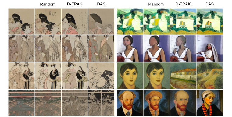
Figure 1: We conduct an visualization experiment to explore DAS effectiveness. We retrain the model after deleting 1000 most influential training samples detected by D-TRAK and DAS. We also add an baseline that randomly delete 1000 samples. From Left to Right, they are the original generated image and generated by retrained model with random deletion, D-TRAK deletion and DAS deletion.

5 Conclusion

In this paper, we introduce the Diffusion Attribution Score (DAS) to address the existing gap in data attribution methodologies for generative models. We conducted a comprehensive theoretical analysis to elucidate the inherent challenges in applying TRAK to diffusion models. Subsequently, we derived DAS theoretically based on the properties of diffusion models for attributing data throughout the entire generation process. We also discuss strategies to accelerate computations to extend DAS to large-scale diffusion models. Our extensive experimental evaluations on datasets such as CIFAR, CelebA, and ArtBench demonstrate that DAS consistently surpasses existing baselines in terms of Linear Datamodeling Score (LDS) evaluation. This paper underscores the crucial role of data attribution in ensuring transparency and fairness in the use of diffusion models, especially when dealing with copyrighted or sensitive content. Looking forward, our future work aims to extend DAS to other generative models and real-world applications to further ascertain its effectiveness and applicability.

Appendix A Related Works

A.1 Data Attribution

The training data exerts a significant influence on the behavior of machine learning models. Data attribution aims to accurately assess the importance of each piece of training data in relation to the desired model outputs. However, methods of data attribution often face the challenge of balancing computational efficiency with accuracy. Sampling-based approaches, such as empirical influence functions (Feldman & Zhang, 2020), Shapley value estimators (Ghorbani & Zou, 2019; Jia et al., 2019), and datamodels (Ilyas et al., 2022), are able to precisely attribute influences to training data but typically necessitate the training of thousands of models to yield dependable results. On the other hand, methods like influence approximation (Koh & Liang, 2017; Schioppa et al., 2022) and gradient agreement scoring (Pruthi et al., 2020) provide computational benefits but may falter in terms of reliability in non-convex settings (Basu et al., 2021; Ilyas et al., 2022; Akyurek et al., 2022).

A.2 Data Attribution in Generative Models

The discussed methods address counterfactual questions within the context of discriminative models, focusing primarily on accuracy and model predictions. Extending these methodologies to generative models presents complexities due to the lack of clear labels or definitive ground truth. Research in this area includes efforts to compute influence within Generative Adversarial Networks (GANs) (Terashita et al., 2021) and Variational Autoencoders (VAEs) (Kong & Chaudhuri, 2021). Recently, Park et al. (2023) developed TRAK, a new attribution method that is both effective and computationally feasible for large-scale models. In the realm of diffusion models, earlier research has explored influence computation by employing ensembles that necessitate training multiple models on varied subsets of training data—a method less suited for traditionally trained models (Dai & Gifford, 2023). Journey TRAK (Georgiev et al., 2023) extends TRAK to diffusion models by attributing influence across individual denoising timesteps. Moreover, D-TRAK (Zheng et al., 2024) has revealed surprising results, indicating that theoretically dubious choices in the design of TRAK might enhance performance, highlighting the imperative for further exploration into data attribution within diffusion models. These studies are pivotal in advancing our understanding and fostering the development of instance-based interpretations in unsupervised learning contexts.

A.3 Application

Recent research has underscored the effectiveness of data attribution methods in a variety of applications. These include explaining model predictions (Koh & Liang, 2017; Ilyas et al., 2022), debugging model behaviors (Shah et al., 2023), assessing the contributions of training data (Ghorbani & Zou, 2019; Jia et al., 2019), identifying poisoned or mislabeled data (Lin et al., 2022), and managing data curation (Khanna et al., 2019; Liu et al., 2021; Jia et al., 2021). Additionally, the adoption of diffusion models in creative industries, as exemplified by Stable Diffusion and its variants, has grown significantly (Rombach et al., 2022; Zhang et al., 2023). This trend highlights the critical need for fair attribution methods that appropriately acknowledge and compensate artists whose works are utilized in training these models. Such methods are also crucial for addressing related legal and privacy concerns (Carlini et al., 2023; Somepalli et al., 2023).

Appendix B Proof of Equation 13

In this section, we provide a detailed proof of Eq. 13. We utilize the Newton Method (Pregibon, 1981) to update the parameters in the diffusion model, where the parameter update $theta^{\prime}$ is defined as:

$$\theta^{\prime}\leftarrow\theta+{\bm{H}}^{-1}_{\theta_{t}}(\mathcal{L}_{\text{Simple}}(\theta))\nabla_{\theta}\mathcal{L}_{\text{Simple}}(\theta)\text{,}$$ (21)

Here, ${\bm{H}}_{\theta_{t}}(\mathcal{L}_{\text{Simple}}(\theta))$ represents the Hessian matrix, and $\nabla_{\theta}\mathcal{L}_{\text{Simple}}$ is the gradient w.r.t the Simple Loss in the diffusion model. At convergence, the model reaches the global optimum parameter estimate $\theta^{*}$, satisfying:

$${\bm{H}}^{-1}_{\theta_{t}}(\mathcal{L}_{\text{Simple}}(\theta^{*}))\nabla_{\theta}\mathcal{L}_{\text{Simple}}(\theta^{*})=0\text{.}$$ (22)

Additionally, the Hessian matrix and gradient associated with the objective function at timestep $t$ are defined as:

$$\mathbf{H}_{\theta^{*}}={\nabla_{\theta}{\bm{\epsilon}}_{\theta^{*}}({\mathbb{S}}_{t},t)}^{\top}\nabla_{\theta}{\bm{\epsilon}}_{\theta^{*}}({\mathbb{S}}_{t},t),\ \nabla_{\theta}\mathcal{L}({\theta^{*}})=\nabla_{\theta}{\bm{\epsilon}}_{\theta^{*}}({\mathbb{S}}_{t},t)^{\top}{\bm{R}}_{t}\text{,}$$ (23)

where ${\bm{\epsilon}}_{\theta^{*}}({\mathbb{S}}_{t},t):=[{\bm{\epsilon}}_{\theta^{*}}({\bm{x}}^{(1)}_{t},t),...,{\bm{\epsilon}}_{\theta^{*}}({\bm{x}}^{(n)}_{t},t)]$ denotes a stacked output matrix on ${\mathbb{S}}$ at timestep $t$ and ${\bm{R}}_{t}:=\text{diag}[{\bm{\epsilon}}_{\theta}({\bm{x}}^{(i)}_{t},t)-{\bm{\epsilon}}]$ is a diagonal matrix on ${\mathbb{S}}$ describing the residual among ${\mathbb{S}}$. Thus, the update defined in Eq. 21 around the optimum parameter$\theta^{*}$ is:

$$\theta^{\prime}-\theta\leftarrow[{\nabla_{\theta}{\bm{\epsilon}}_{\theta^{*}}({\mathbb{S}}_{t},t)}^{\top}\nabla_{\theta}{\bm{\epsilon}}_{\theta^{*}}({\mathbb{S}}_{t},t)]^{-1}\nabla_{\theta}{\bm{\epsilon}}_{\theta^{*}}({\mathbb{S}}_{t},t)^{\top}{\bm{R}}_{t}\text{.}$$ (24)

Upon deleting a training sample ${\bm{x}}^{(i)}$ from ${\mathbb{S}}$, the counterfactual parameters $\theta_{\backslash i}^{*}$ can be estimated by applying a single step of Newton’s method from the optimal parameter $\theta^{*}$ with the modified set ${\mathbb{S}}_{\backslash i}$, as follows:

$$\theta^{*}-\theta^{*}_{\backslash i}\leftarrow-[{\nabla_{\theta}{\bm{\epsilon}}_{\theta^{*}}({{\mathbb{S}}_{\backslash i}}_{t},t)}^{\top}\nabla_{\theta}{\bm{\epsilon}}_{\theta^{*}}({{\mathbb{S}}_{\backslash i}}_{t},t)]^{-1}\nabla_{\theta}{\bm{\epsilon}}_{\theta^{*}}({{\mathbb{S}}_{\backslash i}}_{t},t)^{\top}{{\bm{R}}_{\backslash i}}_{t}\text{.}$$ (25)

Appendix C Proof of Equation 15

In this section, we provide a detailed proof of Eq. 15. The Sherman-Morrison formula is defined as:

$$({\bm{A}}+{\bm{u}}{\bm{v}}^{\top})^{-1}={\bm{A}}^{-1}-\frac{{\bm{A}}^{-1}{\bm{u}}{\bm{v}}^{\top}{\bm{A}}^{-1}}{1+{\bm{v}}^{\top}{\bm{A}}^{-1}{\bm{u}}}\text{.}$$ (26)

Let ${\bm{H}}={\bm{G}}_{t}({\mathbb{S}})^{\top}{\bm{G}}_{t}({\mathbb{S}})$ and ${\bm{u}}={\bm{g}}_{t}({\bm{x}}^{(i)})$. Applying Eq. 26 in Eq. 14, we derive:

$$[{\bm{G}}_{t}({\mathbb{S}}_{\backslash i})^{\top}{\bm{G}}_{t}({\mathbb{S}}_{\backslash i})]^{-1}=[{\bm{H}}-{\bm{u}}{\bm{u}}^{\top}]^{-1}={\bm{H}}^{-1}+\frac{{\bm{H}}^{-1}{\bm{u}}{\bm{u}}^{\top}{\bm{H}}^{-1}}{1-{\bm{u}}^{\top}{\bm{H}}^{-1}{\bm{u}}}\text{.}$$ (27)

Additionally, we have:

$${\bm{G}}_{t}({\mathbb{S}}_{\backslash i})^{\top}{{\bm{R}}_{\backslash i}}_{t}={\bm{G}}_{t}({\mathbb{S}})^{\top}{\bm{R}}_{t}-{\bm{g}}_{t}({\bm{x}}^{(i)})^{\top}{{\bm{r}}^{(i)}}_{t}=-{\bm{u}}^{\top}{{\bm{r}}^{(i)}_{t}}\text{.}$$ (28)

Applying Eq. 27 and Eq. 28 to Eq. 25, we obtain:

$$\theta^{*}-\theta^{*}_{\backslash i}=[{\bm{H}}^{-1}+\frac{{\bm{H}}^{-1}{\bm{u}}{\bm{u}}^{\top}{\bm{H}}^{-1}}{1-{\bm{u}}^{\top}{\bm{H}}^{-1}{\bm{u}}}]{\bm{u}}^{\top}{{\bm{r}}^{(i)}_{t}}\text{.}$$ (29)

Let $\alpha={\bm{u}}^{\top}{\bm{H}}^{-1}{\bm{u}}$. Eq. 29 simplifies to:

$$\theta^{*}-\theta^{*}_{\backslash i} ={\bm{H}}^{-1}{\bm{u}}\cdot(1+\frac{\alpha}{1-\alpha}){{\bm{r}}^{(i)}_{t}}$$

$$={\bm{H}}^{-1}{\bm{u}}\cdot\frac{1}{1-\alpha}{{\bm{r}}^{(i)}_{t}}$$

$$=\frac{[{\bm{G}}_{t}({\mathbb{S}})^{\top}{\bm{G}}_{t}({\mathbb{S}})]^{-1}{\bm{g}}_{t}({\bm{x}}^{(i)}){\bm{r}}^{(i)}_{t}}{1-{\bm{g}}_{t}({\bm{x}}^{(i)})^{\top}[({\bm{G}}_{t}({\mathbb{S}})^{\top}{\bm{G}}_{t}({\mathbb{S}})]^{-1}{\bm{g}}_{t}({\bm{x}}^{(i)})}\text{.}$$ (30)

Appendix D Algorithm of DAS

In this section, we provide a algorithm about DAS in Algorithm 1.

Algorithm 1 Diffusion Attribution Score

1:Input: Learning algorithm $\mathcal{A}$, Training dataset ${\mathbb{S}}$ of size $n$, Training data dimension $p$, Maximum timesteps for diffusion model $T$, Unet output in diffusion model ${\bm{\epsilon}}_{\theta}({\bm{x}},t)$, Projection dimension $k$, A standard gaussian noise ${\bm{\epsilon}}\sim\mathcal{N}(0,{\bm{I}})$, Normalization and average method $N$, A generated sample ${\bm{z}}^{\text{gen}}$

2:Output: Matrix of attribution scores ${\bm{T}}\in{\bm{R}}^{n}$

3:$\theta^{*}\leftarrow\mathcal{A}({\mathbb{S}})$ $\triangleright$ Train a diffusion model on ${\mathbb{S}}$

4:${\bm{P}}\sim\mathcal{N}(0,1)^{p\times k}$ $\triangleright$ Sample projection matrix

5:${\bm{R}}\leftarrow 0_{n\times n}$

6:for $i=1$ to $n$ do

7:     for $t=1$ to $T$ do

8:         ${\bm{\epsilon}}\sim\mathcal{N}(0,1)^{p}$ $\triangleright$ Sample a gaussian noise

9:         ${\bm{g}}_{t}({\bm{x}}^{(i)})\leftarrow{\bm{P}}^{\top}\nabla_{\theta}{\bm{\epsilon}}_{\theta^{*}}({\bm{x}}^{(i)}_{t},t)$ $\triangleright$ Compute gradient on training set and project

10:         ${\bm{r}}^{(i)}_{t}\leftarrow{\bm{\epsilon}}_{\theta^{*}}({\bm{x}}^{(i)}_{t},t)-{\bm{\epsilon}}$ $\triangleright$ Compute residual term

11:     end for

12:     $\overline{{\bm{g}}}({\bm{x}}^{(i)})=N({\bm{g}}_{t}({\bm{x}}^{(i)}))$ $\triangleright$ Normalize projected gradient term

13:     $\overline{{\bm{r}}}^{(i)}=N({\bm{r}}^{(i)}_{t})$ $\triangleright$ Normalize residual term

14:end for

15:$\overline{{\bm{G}}}({\mathbb{S}})\leftarrow[\overline{{\bm{g}}}({\bm{x}}^{(i)}),...,\overline{{\bm{g}}}({\bm{x}}^{(n)})]^{\top}$

16:$\overline{{\bm{R}}}\leftarrow\text{diag}(\overline{{\bm{r}}}^{(1)},...,\overline{{\bm{r}}}^{(n)})$

17:for $t=1$ to $T$ do

18:     ${\bm{\epsilon}}\sim\mathcal{N}(0,1)^{p}$ $\triangleright$ Sample a gaussian noise

19:     ${\bm{g}}_{t}({\bm{x}}^{\text{gen}})\leftarrow{\bm{P}}^{\top}\nabla_{\theta}{\bm{\epsilon}}_{\theta^{*}}({\bm{x}}_{t}^{\text{gen}},t)$ $\triangleright$ Compute gradient for generated sample and project

20:end for

21:$\overline{{\bm{g}}}(x^{\text{gen}})=N({\bm{g}}_{t}(x^{\text{gen}}))$

22:${\bm{T}}\leftarrow||\frac{\overline{{\bm{g}}}(x^{\text{gen}})^{\top}(\overline{{\bm{G}}}({\mathbb{S}})^{\top}\overline{{\bm{G}}}({\mathbb{S}}))^{-1}\overline{{\bm{G}}}({\mathbb{S}})\overline{{\bm{R}}}}{1-\overline{{\bm{G}}}({\mathbb{S}})^{\top}(\overline{{\bm{G}}}({\mathbb{S}})^{\top}\overline{{\bm{G}}}({\mathbb{S}}))^{-1}\overline{{\bm{G}}}({\mathbb{S}})}||^{2}$$\triangleright$ Compute attribution matrix

23:return $(T)$

Appendix E Explanation about the choice of model output function in LDS evaluation

In the LDS framework, we evaluate the ranking correlation between the ground-truth and the predicted model outputs following a data intervention. In our evaluations, the output function used in JourneyTRAK and D-TRAK is shown to provide the same ranking as our DAS output function. Below, we provide a detailed explanation of this alignment.

Defining the function $f({\bm{z}},\theta)$ as $\mathcal{L}_{\text{Simple}}$, D-TRAK predicts the change in output as:

$$f({\bm{z}}^{\text{gen}},\theta)-f({\bm{z}}^{\text{gen}},\theta_{m})=\mathbb{E}_{{\bm{\epsilon}},t}[||{\bm{\epsilon}}-{\bm{\epsilon}}_{\theta}({\bm{z}}^{\text{gen}}_{t},t)||^{2}]-\mathbb{E}_{\bm{\epsilon}}[||{\bm{\epsilon}}-{\bm{\epsilon}}_{\theta_{m}}({\bm{z}}^{\text{gen}}_{t},t)||^{2}]\text{,}$$ (31)

where $\theta$ and $\theta_{m}$ represent the models trained on the full dataset ${\mathbb{S}}$ and a subset ${\mathbb{S}}_{m}$, respectively. With the retraining of the model on subset ${\mathbb{S}}_{m}$ while fixing all randomness, the real change can be computed as:

$$f({\bm{z}}^{\text{gen}},\theta)-f({\bm{z}}^{\text{gen}},\theta_{m})= \mathbb{E}_{{\bm{\epsilon}},t}[||{\bm{\epsilon}}_{\theta}({\bm{z}}^{\text{gen}}_{t},t)-{\bm{\epsilon}}_{\theta_{m}}({\bm{z}}^{\text{gen}}_{t},t)||^{2}]$$

$$+2\mathbb{E}_{\bm{\epsilon}}[({\bm{\epsilon}}_{\theta}({\bm{z}}^{\text{gen}}_{t},t)-{\bm{\epsilon}}_{\theta_{m}}({\bm{z}}^{\text{gen}}_{t},t))\cdot({\bm{\epsilon}}-{\bm{\epsilon}}_{\theta_{m}}({\bm{z}}^{\text{gen}}_{t},t))]\text{.}$$ (32)

The first expectation represents the predicted output change in DAS as well as the ground truth output, while the term $({\bm{\epsilon}}-{\bm{\epsilon}}_{\theta_{m}}({\bm{z}}^{\text{gen}}_{t},t))$ is recognized as the error of the MMSE estimator.

In our evaluations, the sampling noise ${\bm{\epsilon}}$ is fixed and ${\bm{\epsilon}}_{\theta}({\bm{z}}^{\text{gen}}_{t},t)$ is a given value since the model $\theta$ is frozen. Therefore, the second term equals zero, following the orthogonality principle. It can be stated as a more general result that,

$$\forall f\ ,\mathbb{E}[f({\bm{\epsilon}}_{\theta_{m}},{\bm{z}}^{\text{gen}})\cdot({\bm{\epsilon}}-{\bm{\epsilon}}_{\theta_{m}}({\bm{z}}^{\text{gen}}))]=0\text{.}$$ (33)

The error $({\bm{\epsilon}}-{\bm{\epsilon}}_{\theta_{m}}({\bm{z}}^{\text{gen}}))$ must be orthogonal to any estimator $f$. If not, we could use $f$ to construct an estimator with a lower MSE than ${\bm{\epsilon}}_{\theta_{m}}(x_{gen})$, contradicting our assumption that $({\bm{\epsilon}}-{\bm{\epsilon}}_{\theta_{m}}({\bm{z}}^{\text{gen}}))$ is the MMSE estimator. Applications of the orthogonality principle in diffusion models have been similarly proposed (Kong et al., 2024; Banerjee et al., 2005). Thus, given that we have a frozen model $\theta$, fixed sampling noise ${\bm{\epsilon}}$ and a specific generated sample ${\bm{z}}^{\text{gen}}$, the change in the output function in DAS provides the same rank as the one in JourneyTRAK and D-TRAK.

Appendix F Implementation details

F.1 Datasets and Models

CIFAR10(32$\times$32). The CIFAR-10 dataset, introduced by Krizhevsky (2009), consists of 50,000 training images across various classes. For the Linear Datamodeling Score evluation, we utilize a subset of 1,000 images randomly selected from CIFAR-10’s test set. To manage computational demands effectively, we also create a smaller subset, CIFAR-2, which includes 5,000 training images and 1,000 validation images specifically drawn from the ”automobile” and ”horse” categories of CIFAR-10’s training and test sets, respectively.

In our CIFAR experiments, we employ the architecture and settings of the Denoising Diffusion Probabilistic Models (DDPMs) as outlined by Ho et al. (2020). The model is configured with approximately 35.7 million parameters ($d=35.7\times 10^{6}$ for $\theta\in\mathbb{R}^{d}$). We set the maximum number of timesteps ($T$) at 1,000 with a linear variance schedule for the forward diffusion process, beginning at $\beta_{1}=10^{-4}$ and escalating to $\beta_{T}=0.02$. Additional model specifications include a dropout rate of 0.1 and the use of the AdamW optimizer (Loshchilov & Hutter, 2019) with a weight decay of $10^{-6}$. Data augmentation techniques such as random horizontal flips are employed to enhance model robustness. The training process spans 200 epochs with a batch size of 128, using a cosine annealing learning rate schedule that incorporates a warm-up period covering 10% of the training duration, beginning from an initial learning rate of $10^{-4}$. During inference, new images are generated using the 50-step Denoising Diffusion Implicit Models (DDIM) solver (Song et al., 2021a).

CelebA(64$\times$64). We selected 5,000 training samples and 1,000 validation samples from the original training and test sets of CelebA (Liu et al., 2015), respectively. Following the preprocessing method described by Song et al. (2021b), we first center-cropped the images to 140$\times$140 pixels and then resized them to 64$\times$64 pixels. For the CelebA experiments, we adapted the architecture to accommodate a 64$\times$64 resolution while employing a similar unconditional DDPM implementation as used for CIFAR-10. However, the U-Net architecture was expanded to 118.8 million parameters to better capture the increased complexity of the CelebA dataset. The hyperparameters, including the variance schedule, optimizer settings, and training protocol, were kept consistent with those used for the CIFAR-10 experiments.

ArtBench(256$\times$256). ArtBench (Liao et al., 2022) is a dataset specifically designed for generating artwork, comprising 60,000 images across 10 unique artistic styles. Each style contributes 5,000 training images and 1,000 testing images. We introduce two subsets from this dataset for focused evaluation: ArtBench-2 and ArtBench-5. ArtBench-2 features 5,000 training and 1,000 validation images selected from the ”post-impressionism” and ”ukiyo-e” styles, extracted from a total of 10,000 training and 2,000 test images. ArtBench-5 includes 12,500 training and 1,000 validation images drawn from a larger pool of 25,000 training and 5,000 test images across five styles: ”post-impressionism,” ”ukiyo-e,” ”romanticism,” ”renaissance,” and ”baroque.”

For our experiments on ArtBench, we fine-tune a Stable Diffusion model (Rombach et al., 2022) using Low-Rank Adaptation (LoRA) (Hu et al., 2022) with a rank of 128, amounting to 25.5 million parameters. We adapt a pre-trained Stable Diffusion checkpoint from a resolution of 512$\times$512 to 256$\times$256 to align with the ArtBench specifications. The model is trained conditionally using textual prompts specific to each style, such as ”a class painting,” e.g., ”a romanticism painting.” We set the dropout rate at 0.1 and employ the AdamW optimizer with a weight decay of $10^{-6}$. Data augmentation is performed via random horizontal flips. The training is conducted over 100 epochs with a batch size of 64, under a cosine annealing learning rate schedule that includes a 0.1 fraction warm-up period starting from an initial rate of $3\times 10^{-4}$. During the inference phase, we generate new images using the 50-step DDIM solver with a classifier-free guidance scale of 7.5 (Ho & Salimans, 2021).

F.2 LDS evaluation setup

For the LDS evaluation, we construct 64 distinct subsets ${\mathbb{S}}_{m}$ from the training dataset ${\mathbb{S}}$, each constituting 50% of the total training set size. To ensure robustness and mitigate any effects of randomness, three separate models are trained on each subset using different random seeds. The LDS is computed by measuring the Spearman rank correlation between the model outputs and the attribution-based output predictions for selected samples. Specifically, we evaluate the Simple Loss $\mathcal{L}_{\text{Simple}}({\bm{z}},\theta)$ as defined in Eq 3 for samples of interest from both the validation and generation sets. To better approximate the expectation $\mathbb{E}_{t}$, we utilize 1,000 timesteps, evenly spaced within the range $[1,T]$. At each timestep, three instances of standard Gaussian noise ${\bm{\epsilon}}\sim\mathcal{N}(0,{\bm{I}})$ are introduced to approximate the expectation $\mathbb{E}_{\bm{\epsilon}}$. The calculated LDS values are then averaged across the selected samples from both the validation and generation sets to determine the overall LDS performance.

F.3 Baselines

In this paper, our focus is primarily on post-hoc data attribution, which entails applying attribution methods after the completion of model training. These methods are particularly advantageous as they do not impose additional constraints during the model training phase, making them well-suited for practical applications (Ribeiro et al., 2016).

Following the work of Hammoudeh & Lowd (2024), we evaluate various attribution baselines that are compatible with our experimental framework. We exclude certain methods that are not feasible for our settings, such as the Leave-One-Out approach (Cook, 1977) and the Shapley Value method (Shapley et al., 1953; Ghorbani & Zou, 2019). These methods, although foundational, do not align well with the requirements of DDPMs due to their intensive computational demands and model-specific limitations. Additionally, we do not consider techniques like Representer Point (Yeh et al., 2018), which are tailored for specific tasks and models, and thus are incompatible with DDPMs. Moreover, we disregard HYDRA (Chen et al., 2021), which, although related to TracInCP (Pruthi et al., 2020), compromises precision for incremental speed improvements as critiqued by Hammoudeh & Lowd (2024).

Two works focus on diffusion model that also fall outside our framework. Dai & Gifford (2023) propose a method for training data attribution on diffusion models using machine unlearning (Bourtoule et al., 2021); however, their approach necessitates a specific machine unlearning training process, making it non-post-hoc and thus unsuitable for standard settings. Similarly, Wang et al. (2023) acknowledge the current challenges in conducting post-hoc training influence analysis with existing methods. They suggest an alternative termed ”customization,” which involves adapting or tuning a pretrained text-to-image model through a specially designed training procedure.

Building upon recent advancements, Park et al. (2023) introduced an innovative estimator that leverages a kernel matrix analogous to the Fisher Information Matrix (FIM), aiming to linearize the model’s behavior. This approach integrates classical random projection techniques to expedite the computation of Hessian-based influence functions (Koh & Liang, 2017), which are typically computationally intensive. Zheng et al. (2024) adapted TRAK to diffusion models, empirically designing the model output function. Intriguingly, they reported that the theoretically designed model output function in TRAK performs poorly in unsupervised settings within diffusion models. However, they did not provide a theoretical explanation for these empirical findings, leaving a gap in understanding the underlying mechanics.

Our study concentrates on retraining-free methods, which we categorize into three distinct types: similarity-based, gradient-based (without kernel), and gradient-based (with kernel) methods. For similarity-based approaches, we consider Raw pixel similarity and CLIP similarity (Radford et al., 2021). The gradient-based methods without a kernel include techniques such as Gradient (Charpiat et al., 2019), TracInCP (Pruthi et al., 2020) and GAS (Hammoudeh & Lowd, 2022). In the domain of gradient-based methods with a kernel, we explore several methods including D-TRAK (Zheng et al., 2024), TRAK (Park et al., 2023), Relative Influence (Barshan et al., 2020), Renormalized Influence (Hammoudeh & Lowd, 2022), and Journey TRAK (Georgiev et al., 2023).

We next provide definition and implementation details of the baselines used in Section 4.4.

Raw pixel. This method employs a naive similarity-based approach for data attribution by using the raw image data itself as the representation. Specifically, for experiments on ArtBench, which utilizes latent diffusion models (Rombach et al., 2022), we represent the images through the VAE encodings (Van Den Oord et al., 2017) of the raw image. The attribution score is calculated by computing either the dot product or cosine similarity between the sample of interest and each training sample, facilitating a straightforward assessment of similarity based on pixel values.

CLIP Similarity. This method represents another similarity-based approach to data attribution. Each sample is encoded into an embedding using the CLIP model (Radford et al., 2021), which captures semantic and contextual nuances of the visual content. The attribution score is then determined by computing either the dot product or cosine similarity between the CLIP embedding of the target sample and those of the training samples. This method leverages the rich representational power of CLIP embeddings to ascertain the contribution of training samples to the generation or classification of new samples.

Gradient. This method employs a gradient-based approach to estimate the influence of training samples, as described by Charpiat et al. (2019). The attribution score is calculated by taking the dot product or cosine similarity between the gradients of the sample of interest and those of each training sample. This technique quantifies how much the gradient (indicative of the training sample’s influence on the loss) of a particular training sample aligns with the gradient of the sample of interest, providing insights into which training samples most significantly affect the model’s output.

$$\begin{split}&\tau({\bm{z}},{\mathbb{S}})^{i}=({\bm{P}}^{\top}\nabla_{\theta}\mathcal{L}_{\text{Simple}}({\bm{x}},\theta))^{\top}\cdot({\bm{P}}^{\top}\nabla_{\theta}\mathcal{L}_{\text{Simple}})({\bm{x}}^{(i)},\theta^{*})\text{,}\\ &\tau({\bm{z}},{\mathbb{S}})^{i}=\frac{({\bm{P}}^{\top}\nabla_{\theta}\mathcal{L}_{\text{Simple}}({\bm{x}},\theta))^{\top}\cdot({\bm{P}}^{\top}\nabla_{\theta}\mathcal{L}_{\text{Simple}}({\bm{x}}^{(i)},\theta))}{||{\bm{P}}^{\top}\nabla_{\theta}\mathcal{L}_{\text{Simple}}({\bm{x}},\theta)||^{\top}||{\bm{P}}^{\top}\nabla_{\theta}\mathcal{L}_{\text{Simple}}({\bm{x}}^{(i)},\theta)||}\text{.}\end{split}$$

TracInCP. We implement the TracInCP estimator, as outlined by Pruthi et al. (2020), which quantifies the influence of training samples using the following formula:

$$\tau({\bm{z}},{\mathbb{S}})^{i}=\frac{1}{C}\Sigma^{C}_{c=1}({\bm{P}}_{c}^{\top}\nabla_{\theta}\mathcal{L}_{\text{Simple}}({\bm{x}},\theta^{c}))^{\top}\cdot({\bm{P}}_{c}^{\top}\nabla_{\theta}\mathcal{L}_{\text{Simple}}({\bm{x}}^{i},\theta^{c}))\text{,}$$

where $C$ represents the number of model checkpoints selected evenly from the training trajectory, and $\theta^{c}$ denotes the model parameters at each checkpoint. For our analysis, we select four specific checkpoints along the training trajectory to ensure a comprehensive evaluation of the influence over different phases of learning. For example, in the CIFAR-2 experiment, the chosen checkpoints occur at epochs 50, 100, 150, and 200, capturing snapshots of the model’s development and adaptation.

GAS. The GAS method is essentially a ”renormalized” version of TracInCP that employs cosine similarity for estimating influence, rather than relying on raw dot products. This method was introduced by Hammoudeh & Lowd (2022) and aims to refine the estimation of influence by normalizing the gradients. This approach allows for a more nuanced comparison between gradients, considering not only their directions but also normalizing their magnitudes to focus solely on the directionality of influence.

TRAK. The retraining-free version of TRAK (Park et al., 2023) utilizes a model’s trained state to estimate the influence of training samples without the need for retraining the model at each evaluation step. This version is implemented using the following equations:

$$\begin{split}&{\bm{\Phi}}_{\text{TRAK}}=\left[{\bm{\Phi}}({\bm{x}}^{1}),\cdots,{\bm{\Phi}}({\bm{x}}^{N})\right]^{\top}\text{, where }{\bm{\Phi}}({\bm{x}})={\bm{P}}^{\top}\nabla_{\theta}\mathcal{L}_{\text{Simple}}({\bm{x}},\theta)\text{,}\\ &\tau({\bm{z}},{\mathbb{S}})^{i}=({\bm{P}}^{\top}\nabla_{\theta}\mathcal{L}_{\text{Simple}}({\bm{x}},\theta))^{\top}\cdot\left({{\bm{\Phi}}_{\text{TRAK}}}^{\top}{\bm{\Phi}}_{\text{TRAK}}+\lambda{\bm{I}}\right)^{-1}\cdot{\bm{P}}^{\top}\nabla_{\theta}\mathcal{L}_{\text{Simple}}({\bm{x}}^{i},\theta)\text{,}\end{split}$$

where $\lambda{\bm{I}}$ is included for numerical stability and regularization. The impact of this term is further explored in Appendix G.

D-TRAK. Simliar to TRAK, as elaborated in Section 2, we adapt the D-TRAK (Zheng et al., 2024) as detailed in Eq 6. We implent the model output function $f({\bm{z}},\theta)$ as $\mathcal{L}_{\text{Square}}$. The D-TRAK is implemented using the following equations:

$$\begin{split}&{\bm{\Phi}}_{\text{D-TRAK}}=\left[{\bm{\Phi}}({\bm{x}}^{1}),\cdots,{\bm{\Phi}}({\bm{x}}^{N})\right]^{\top}\text{, where }{\bm{\Phi}}({\bm{x}})={\bm{P}}^{\top}\nabla_{\theta}\mathcal{L}_{\text{Simple}}({\bm{x}},\theta)\text{,}\\ &\tau({\bm{z}},{\mathbb{S}})^{i}=({\bm{P}}^{\top}\nabla_{\theta}\mathcal{L}_{\text{Simple}}({\bm{x}},\theta))^{\top}\cdot\left({{\bm{\Phi}}_{\text{TRAK}}}^{\top}{\bm{\Phi}}_{\text{TRAK}}+\lambda{\bm{I}}\right)^{-1}\cdot{\bm{P}}^{\top}\nabla_{\theta}\mathcal{L}_{\text{Simple}}({\bm{x}}^{i},\theta)\text{,}\end{split}$$

where $\lambda I$ is also included for numerical stability and regularization as TRAK. Additionally, the output function $f({\bm{z}},\theta)$ could be replaced to other functions.

Relative Influence. Barshan et al. (2020) introduce the $\theta$-relative influence functions estimator, which normalizes the influence functions estimator from Koh & Liang (2017) by the magnitude of the Hessian-vector product (HVP). This normalization enhances the interpretability of influence scores by adjusting for the impact magnitude. We have adapted this method to our experimental framework by incorporating scalability optimizations from TRAK. The adapted equation for the Relative Influence is formulated as follows:

$$\tau({\bm{z}},{\mathbb{S}})^{(i)}=\frac{({\bm{P}}^{\top}\nabla_{\theta}\mathcal{L}_{\text{Simple}}({\bm{x}},\theta))^{\top}\cdot\left({{\bm{\Phi}}_{\text{ TRAK}}}^{\top}{\bm{\Phi}}_{\text{ TRAK}}+\lambda{\bm{I}}\right)^{-1}\cdot{\bm{P}}^{\top}\nabla_{\theta}\mathcal{L}_{\text{Simple}}({\bm{x}}^{(i)},\theta^{*})}{||\left({{\bm{\Phi}}_{\text{TRAK}}}^{\top}{\bm{\Phi}}_{\text{ TRAK}}+\lambda I\right)^{-1}\cdot{\bm{P}}^{\top}\nabla_{\theta}\mathcal{L}_{\text{Simple}}({\bm{x}}^{(i)},\theta^{*})||}\text{.}$$

Renormalized Influence. Hammoudeh & Lowd (2022) propose a method to renormalize influence by considering the magnitude of the training sample’s gradients. This approach emphasizes the relative strength of each sample’s impact on the model, making the influence scores more interpretable and contextually relevant. We have adapted this method to our settings by incorporating TRAK’s scalability optimizations, which are articulated as:

$$\tau({\bm{z}},{\mathbb{S}})^{(i)}=\frac{({\bm{P}}^{\top}\nabla_{\theta}\mathcal{L}_{\text{Simple}}({\bm{x}},\theta))^{\top}\cdot\left({{\bm{\Phi}}_{\text{ TRAK}}}^{\top}{\bm{\Phi}}_{\text{ TRAK}}+\lambda{\bm{I}}\right)^{-1}\cdot{\bm{P}}^{\top}\nabla_{\theta}\mathcal{L}_{\text{Simple}}({\bm{x}}^{(i)},\theta)}{||{\bm{P}}^{\top}\nabla_{\theta}\mathcal{L}_{\text{Simple}}({\bm{x}}^{(i)},\theta)||}\text{.}$$

Journey TRAK. Journey TRAK (Georgiev et al., 2023) focuses on attributing influence to noisy images ${\bm{x}}_{t}$ at a specific timestep $t$ throughout the generative process. In contrast, our approach aims to attribute the final generated image ${\bm{x}}^{\text{gen}}$, necessitating an adaptation of their method to our context. We average the attributions across the generation timesteps, detailed in the following equation:

$$\tau({\bm{z}},{\mathbb{S}})^{(i)}=\frac{1}{T^{\prime}}\Sigma^{T^{\prime}}_{t=1}({\bm{P}}^{\top}\nabla_{\theta}\mathcal{L}^{t}_{\text{Simple}}({\bm{x}}_{t},\theta))^{\top}\cdot\left({{\bm{\Phi}}_{\text{ TRAK}}}^{\top}{\bm{\Phi}}_{\text{ TRAK}}+\lambda{\bm{I}}\right)^{-1}\cdot{\bm{P}}^{\top}\nabla_{\theta}\mathcal{L}_{\text{Simple}}({\bm{x}}^{(i)},\theta)\text{,}$$

where $T^{\prime}$ represents the number of inference steps, set at $50$, and ${\bm{x}}_{t}$ denotes the noisy image generated along the sampling trajectory.

F.4 Experiments Result

In this subsection, we present the outcomes of experiments detailed in Section 4.3. The results, which illustrate the effectiveness of various techniques designed to expedite computational processes in data attribution, are summarized in several tables and figures. These include Table 4, Table 5, Table 6, and Table 7, as well as Figure 2. Each of these displays key findings relevant to the specific speed-up technique tested, providing a comprehensive view of their impacts on attribution performance.

Table 4: We compare D-TRAK and our methods DAS with the normalization and without normalization on CIFAR2. Besides, we also select 10, 100 and 1000 timesteps evenly spaced within the interval $[1,T]$ and calculate the average of LDS(%) among the timesteps.

Method	Normalization	Validation			Generation
		10	100	1000	10	100	1000
D-TRAK	No Normalization	24.78	30.81	32.37	16.20	22.62	23.94
	Normalization	26.11	31.50	32.51	17.09	22.92	24.10
DAS	No Normalization	33.04	42.02	43.13	20.01	29.58	30.58
	Normalization	33.77	42.26	43.28	21.24	29.60	30.87

Table 5: We compare our methods with TRAK and D-TRAK by LDS method on CIFAR-2 among different selected timesteps. The projected dimension $k=4096$.

Method	Validation			Generation
	10	100	1000	10	100	1000
TRAK	10.66	19.50	22.42	5.14	12.05	15.46
D-TRAK	24.91	30.91	32.39	16.76	22.62	23.94
DAS	33.04	42.02	43.13	20.01	29.58	30.58

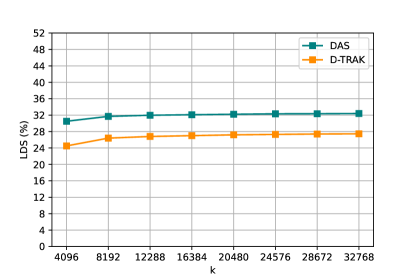
(a) Val-10

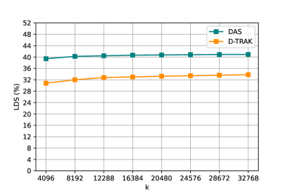
(b) Val-100

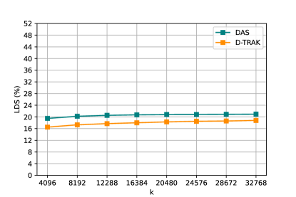
(c) Gen-10

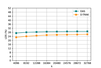
(d) Val-100

Figure 2: The LDS(%) on CIFAR-2 under different projection dimension $k$. We consider 10 and 100 timesteps selected to be evenly spaced within the interval $[1,T]$, which are used to approximate the expectation $\mathbb{E}_{t}$. For each sampled timestep, we sample one standard Gaussian noise $\epsilon\sim\mathcal{N}(\epsilon|0,I)$ to approximate the expectation $\mathbb{E}_{\epsilon}$.

Table 6: We compute DAS only with the Up-Block gradients in U-Net and evaluate by LDS method on CIFAR-2 among different selected timesteps. The projected dimension $k=32768$.

Method	Validation		Generation
	10	100	10	100
D-TRAK	24.91	30.91	16.76	22.62
DAS(Up-Block)	32.60	37.90	18.47	27.54
DAS(U-Net)	33.77	42.26	21.24	29.60

Table 7: We compute DAS only with the Up-Block gradients in U-Net and evaluate by LDS method on CIFAR-2 among different selected timesteps. The projected dimension $k=32768$.

Method	Validation		Generation
	10	100	10	100
D-TRAK	24.91	30.91	16.76	22.62
DAS(Candidate Set)	31.53	37.75	17.73	23.31
DAS(Entire Training Set)	33.77	42.26	21.24	29.60

Appendix G Ablation Studies

We conduct additional ablation studies to evaluate the performance differences between D-TRAK and DAS. In this section, CIFAR-2 serves as our primary setting. Further details on these settings are available in Appendix F.1. We establish the corresponding LDS benchmarks as outlined in Appendix F.2.

Checkpoint selection Following the approach outlined by Pruthi et al. (2020), we investigated the impact of utilizing different model checkpoints for gradient computation. As depicted in Figures 3, our method achieves the highest LDS when utilizing the final checkpoint. This finding suggests that the later stages of model training provide the most accurate reflections of data influence, aligning gradients more closely with the ultimate model performance. Determining the optimal checkpoint for achieving the best LDS score requires multiple attributions to be computed, which significantly increases the computational expense. Additionally, in many practical scenarios, access may be limited exclusively to the final model checkpoint. This constraint highlights the importance of developing efficient methods that can deliver precise attributions even when earlier checkpoints are not available.

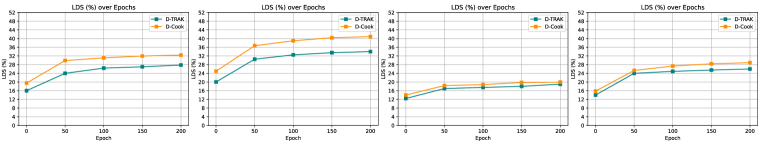
Figure 3: The LDS(%) on CIFAR-2 varies across different checkpoints. We analyze the data using 10 and 100 timesteps, evenly spaced within the interval $[1,T]$, to approximate the expectation $\mathbb{E}_{t}$. At each sampled timestep, we introduce one standard Gaussian noise $\bm{\epsilon}\sim\mathcal{N}(\mathbf{0},\mathbf{I})$ to approximate the expectation $\mathbb{E}_{\epsilon}$. We set the projection dimension $k=32768$.

Value of $\lambda$ In our computation of the inverse of the Hessian matrix within the DAS framework, we incorporate the regularization parameter $\lambda$, as recommended by Hastie (2020), to ensure numerical stability and effective regularization. Traditionally, $\lambda$ is set to a value close to zero; however, in our experiments, a larger $\lambda$ proved necessary, possibly due to the absence of normalization by the number of training samples $N$ in the kernel (Park et al., 2023).

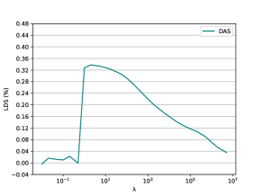
(a) VAl-10

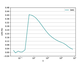
(b) VAl-100

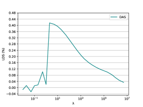
(c) VAl-1000

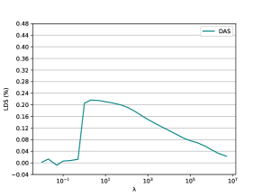
(d) GEN-10

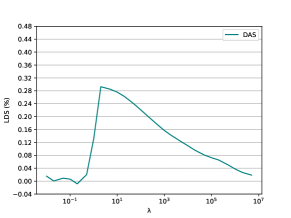
(e) GEN-100

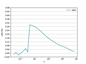
(f) GEN-1000

Figure 4: LDS (%) on CIFAR-2 under different $\lambda$. We consider 10, 100, and 1000 timesteps selected to be evenly spaced within the interval $[1,T]$, which are used to approximate the expectation $\mathbb{E}_{t}$. We set $k=4096$.

Appendix H Limitations and Broader Impacts

H.1 Limitations

While our proposed Diffusion Attribution Score (DAS) showcases notable improvements in data attribution for diffusion models, several limitations warrant attention. Firstly, although DAS reduces the computational load compared to traditional methods, it still demands significant resources due to the requirement to train multiple models and compute extensive gradients. This poses challenges particularly for large-scale models and expansive datasets. Secondly, the current implementation of DAS is tailored primarily to image generation tasks. Its effectiveness and applicability to other forms of generative models, such as those for generating text or audio, remain untested and may not directly translate. Furthermore, DAS operates under the assumption that the influence of individual training samples is additive. This simplification may not accurately reflect the complex interactions and dependencies that can exist between samples within the training data.

H.2 Broader Impacts

The advancement of robust data attribution methods like DAS carries substantial ethical and practical implications. By enabling a more transparent linkage between generated outputs and their corresponding training data, DAS enhances the accountability of generative models. Such transparency is crucial in applications involving copyrighted or sensitive materials, where clear attribution supports intellectual property rights and promotes fairness. Nonetheless, the capability to trace back to the data origins also introduces potential privacy risks. It could allow for the identification and extraction of information pertaining to specific training samples, thus raising concerns about the privacy of data contributors. This highlights the necessity for careful handling of data privacy and security in the deployment of attribution techniques. The development of DAS thus contributes positively to the responsible use and governance of generative models, aligning with ethical standards and fostering greater trust in AI technologies. Moving forward, it is imperative to continue exploring these ethical dimensions, particularly the balance between transparency and privacy. Ensuring that advancements in data attribution go hand in hand with stringent privacy safeguards will be essential in maintaining the integrity and trustworthiness of AI systems.

References

- Akyurek et al. (2022) Ekin Akyurek, Tolga Bolukbasi, Frederick Liu, Binbin Xiong, Ian Tenney, Jacob Andreas, and Kelvin Guu. Towards tracing knowledge in language models back to the training data. In Findings of the Association for Computational Linguistics: EMNLP 2022. Association for Computational Linguistics, 2022.
- Banerjee et al. (2005) Arindam Banerjee, Srujana Merugu, Inderjit S Dhillon, Joydeep Ghosh, and John Lafferty. Clustering with bregman divergences. Journal of machine learning research, 2005.
- Barshan et al. (2020) Elnaz Barshan, Marc-Etienne Brunet, and Gintare Karolina Dziugaite. Relatif: Identifying explanatory training samples via relative influence. In International Conference on Artificial Intelligence and Statistics, 2020.
- Basu et al. (2021) Samyadeep Basu, Phil Pope, and Soheil Feizi. Influence functions in deep learning are fragile. In International Conference on Learning Representations, 2021.
- Bourtoule et al. (2021) Lucas Bourtoule, Varun Chandrasekaran, Christopher A. Choquette-Choo, Hengrui Jia, Adelin Travers, Baiwu Zhang, David Lie, and Nicolas Papernot. Machine unlearning. In 2021 IEEE Symposium on Security and Privacy (SP), 2021.
- Carlini et al. (2023) Nicolas Carlini, Jamie Hayes, Milad Nasr, Matthew Jagielski, Vikash Sehwag, Florian Tramer, Borja Balle, Daphne Ippolito, and Eric Wallace. Extracting training data from diffusion models. In 32nd USENIX Security Symposium (USENIX Security 23), 2023.
- Charpiat et al. (2019) Guillaume Charpiat, Nicolas Girard, Loris Felardos, and Yuliya Tarabalka. Input similarity from the neural network perspective. Advances in Neural Information Processing Systems, 2019.
- Chen et al. (2021) Yuanyuan Chen, Boyang Li, Han Yu, Pengcheng Wu, and Chunyan Miao. Hydra: Hypergradient data relevance analysis for interpreting deep neural networks. In Proceedings of the AAAI Conference on Artificial Intelligence, 2021.
- Cook (1977) R Dennis Cook. Detection of influential observation in linear regression. Technometrics, 1977.
- Dai & Gifford (2023) Zheng Dai and David K Gifford. Training data attribution for diffusion models, 2023.
- Feldman & Zhang (2020) Vitaly Feldman and Chiyuan Zhang. What neural networks memorize and why: Discovering the long tail via influence estimation. Advances in Neural Information Processing Systems, 2020.
- Georgiev et al. (2023) Kristian Georgiev, Joshua Vendrow, Hadi Salman, Sung Min Park, and Aleksander Madry. The journey, not the destination: How data guides diffusion models. In Arxiv preprint arXiv:2312.06205, 2023.
- Ghorbani & Zou (2019) Amirata Ghorbani and James Zou. Data shapley: Equitable valuation of data for machine learning. In International conference on machine learning, 2019.
- Hammoudeh & Lowd (2022) Zayd Hammoudeh and Daniel Lowd. Identifying a training-set attack’s target using renormalized influence estimation. In Proceedings of the 2022 ACM SIGSAC Conference on Computer and Communications Security, 2022.
- Hammoudeh & Lowd (2024) Zayd Hammoudeh and Daniel Lowd. Training data influence analysis and estimation: a survey. Machine Learning, 2024.
- Hastie (2020) Trevor Hastie. Ridge regularization: An essential concept in data science. Technometrics, 2020.
- Hertz et al. (2023) Amir Hertz, Ron Mokady, Jay Tenenbaum, Kfir Aberman, Yael Pritch, and Daniel Cohen-or. Prompt-to-prompt image editing with cross-attention control. In The Eleventh International Conference on Learning Representations, 2023.
- Ho & Salimans (2021) Jonathan Ho and Tim Salimans. Classifier-free diffusion guidance. In NeurIPS 2021 Workshop on Deep Generative Models and Downstream Applications, 2021.
- Ho et al. (2020) Jonathan Ho, Ajay Jain, and Pieter Abbeel. Denoising diffusion probabilistic models. Advances in neural information processing systems, 2020.
- Ho et al. (2022) Jonathan Ho, William Chan, Chitwan Saharia, Jay Whang, Ruiqi Gao, Alexey Gritsenko, Diederik P Kingma, Ben Poole, Mohammad Norouzi, David J Fleet, et al. Imagen video: High definition video generation with diffusion models. arXiv preprint arXiv:2210.02303, 2022.
- Hu et al. (2022) Edward J Hu, yelong shen, Phillip Wallis, Zeyuan Allen-Zhu, Yuanzhi Li, Shean Wang, Lu Wang, and Weizhu Chen. LoRA: Low-rank adaptation of large language models. In International Conference on Learning Representations, 2022.
- Ilyas et al. (2022) Andrew Ilyas, Sung Min Park, Logan Engstrom, Guillaume Leclerc, and Aleksander Madry. Datamodels: Predicting predictions from training data. In ICML, 2022.
- Jacot et al. (2018) Arthur Jacot, Franck Gabriel, and Clément Hongler. Neural tangent kernel: Convergence and generalization in neural networks. Advances in neural information processing systems, 2018.
- Jia et al. (2019) Ruoxi Jia, David Dao, Boxin Wang, Frances Ann Hubis, Nick Hynes, Nezihe Merve Gürel, Bo Li, Ce Zhang, Dawn Song, and Costas J Spanos. Towards efficient data valuation based on the shapley value. In The 22nd International Conference on Artificial Intelligence and Statistics, 2019.
- Jia et al. (2021) Ruoxi Jia, Fan Wu, Xuehui Sun, Jiacen Xu, David Dao, Bhavya Kailkhura, Ce Zhang, Bo Li, and Dawn Song. Scalability vs. utility: Do we have to sacrifice one for the other in data importance quantification? In Proceedings of the IEEE/CVF Conference on Computer Vision and Pattern Recognition, 2021.
- Johnson & Lindenstrauss (1984) William Johnson and Joram Lindenstrauss. Extensions of lipschitz maps into a hilbert space. Contemporary Mathematics, 1984.
- Khanna et al. (2019) Rajiv Khanna, Been Kim, Joydeep Ghosh, and Sanmi Koyejo. Interpreting black box predictions using fisher kernels. In The 22nd International Conference on Artificial Intelligence and Statistics, 2019.
- Koh & Liang (2017) Pang Wei Koh and Percy Liang. Understanding black-box predictions via influence functions. In International conference on machine learning, 2017.
- Kong et al. (2024) Xianghao Kong, Ollie Liu, Han Li, Dani Yogatama, and Greg Ver Steeg. Interpretable diffusion via information decomposition. In The Twelfth International Conference on Learning Representations, 2024.
- Kong & Chaudhuri (2021) Zhifeng Kong and Kamalika Chaudhuri. Understanding instance-based interpretability of variational auto-encoders. Advances in Neural Information Processing Systems, 2021.
- Krizhevsky (2009) A Krizhevsky. Learning multiple layers of features from tiny images. Master’s thesis, University of Tront, 2009.
- Li et al. (2022) Xiang Li, John Thickstun, Ishaan Gulrajani, Percy S Liang, and Tatsunori B Hashimoto. Diffusion-lm improves controllable text generation. Advances in Neural Information Processing Systems, 2022.
- Liao et al. (2022) Peiyuan Liao, Xiuyu Li, Xihui Liu, and Kurt Keutzer. The artbench dataset: Benchmarking generative models with artworks, 2022.
- Lin et al. (2022) Jinkun Lin, Anqi Zhang, Mathias Lécuyer, Jinyang Li, Aurojit Panda, and Siddhartha Sen. Measuring the effect of training data on deep learning predictions via randomized experiments. In International Conference on Machine Learning, 2022.
- Liu et al. (2021) Zhuoming Liu, Hao Ding, Huaping Zhong, Weijia Li, Jifeng Dai, and Conghui He. Influence selection for active learning. In Proceedings of the IEEE/CVF international conference on computer vision, 2021.
- Liu et al. (2015) Ziwei Liu, Ping Luo, Xiaogang Wang, and Xiaoou Tang. Deep learning face attributes in the wild. In Proceedings of the IEEE international conference on computer vision, 2015.
- Loshchilov & Hutter (2019) Ilya Loshchilov and Frank Hutter. Decoupled weight decay regularization. In International Conference on Learning Representations, 2019.
- Lundberg & Lee (2017) Scott M Lundberg and Su-In Lee. A unified approach to interpreting model predictions. Advances in neural information processing systems, 2017.
- Ma et al. (2024) Xinyin Ma, Gongfan Fang, and Xinchao Wang. Deepcache: Accelerating diffusion models for free. In Proceedings of the IEEE/CVF Conference on Computer Vision and Pattern Recognition, pp. 15762–15772, 2024.
- Malladi et al. (2023) Sadhika Malladi, Alexander Wettig, Dingli Yu, Danqi Chen, and Sanjeev Arora. A kernel-based view of language model fine-tuning. In International Conference on Machine Learning, 2023.
- Park et al. (2023) Sung Min Park, Kristian Georgiev, Andrew Ilyas, Guillaume Leclerc, and Aleksander Madry. Trak: Attributing model behavior at scale. In International Conference on Machine Learning, 2023.
- Pregibon (1981) Daryl Pregibon. Logistic regression diagnostics. The annals of statistics, 1981.
- Pruthi et al. (2020) Garima Pruthi, Frederick Liu, Satyen Kale, and Mukund Sundararajan. Estimating training data influence by tracing gradient descent. Advances in Neural Information Processing Systems, 2020.
- Radford et al. (2021) Alec Radford, Jong Wook Kim, Chris Hallacy, Aditya Ramesh, Gabriel Goh, Sandhini Agarwal, Girish Sastry, Amanda Askell, Pamela Mishkin, Jack Clark, et al. Learning transferable visual models from natural language supervision. In International conference on machine learning, 2021.
- Ribeiro et al. (2016) Marco Tulio Ribeiro, Sameer Singh, and Carlos Guestrin. Model-agnostic interpretability of machine learning, 2016.
- Rombach et al. (2022) Robin Rombach, Andreas Blattmann, Dominik Lorenz, Patrick Esser, and Björn Ommer. High-resolution image synthesis with latent diffusion models. In Proceedings of the IEEE/CVF conference on computer vision and pattern recognition, 2022.
- Saharia et al. (2022) Chitwan Saharia, William Chan, Huiwen Chang, Chris Lee, Jonathan Ho, Tim Salimans, David Fleet, and Mohammad Norouzi. Palette: Image-to-image diffusion models. In ACM SIGGRAPH 2022 conference proceedings, 2022.
- Schioppa et al. (2022) Andrea Schioppa, Polina Zablotskaia, David Vilar, and Artem Sokolov. Scaling up influence functions. In Proceedings of the AAAI Conference on Artificial Intelligence, 2022.
- Shah et al. (2023) Harshay Shah, Sung Min Park, Andrew Ilyas, and Aleksander Madry. Modeldiff: A framework for comparing learning algorithms. In International Conference on Machine Learning, 2023.
- Shapley et al. (1953) Lloyd S Shapley et al. A value for n-person games. Machine Learning, 1953.
- Somepalli et al. (2023) Gowthami Somepalli, Vasu Singla, Micah Goldblum, Jonas Geiping, and Tom Goldstein. Diffusion art or digital forgery? investigating data replication in diffusion models. In Proceedings of the IEEE/CVF Conference on Computer Vision and Pattern Recognition, 2023.
- Song et al. (2021a) Jiaming Song, Chenlin Meng, and Stefano Ermon. Denoising diffusion implicit models. In International Conference on Learning Representations, 2021a.
- Song et al. (2021b) Yang Song, Jascha Sohl-Dickstein, Diederik P Kingma, Abhishek Kumar, Stefano Ermon, and Ben Poole. Score-based generative modeling through stochastic differential equations. In International Conference on Learning Representations, 2021b.
- Terashita et al. (2021) Naoyuki Terashita, Hiroki Ohashi, Yuichi Nonaka, and Takashi Kanemaru. Influence estimation for generative adversarial networks. In International Conference on Learning Representations, 2021.
- Van Den Oord et al. (2017) Aaron Van Den Oord, Oriol Vinyals, et al. Neural discrete representation learning. Advances in neural information processing systems, 2017.
- Wang et al. (2023) Sheng-Yu Wang, Alexei A Efros, Jun-Yan Zhu, and Richard Zhang. Evaluating data attribution for text-to-image models. In Proceedings of the IEEE/CVF International Conference on Computer Vision, 2023.
- Yeh et al. (2018) Chih-Kuan Yeh, Joon Kim, Ian En-Hsu Yen, and Pradeep K Ravikumar. Representer point selection for explaining deep neural networks. Advances in neural information processing systems, 2018.
- Zhang et al. (2023) Lvmin Zhang, Anyi Rao, and Maneesh Agrawala. Adding conditional control to text-to-image diffusion models. In Proceedings of the IEEE/CVF International Conference on Computer Vision, 2023.
- Zheng et al. (2024) Xiaosen Zheng, Tianyu Pang, Chao Du, Jing Jiang, and Min Lin. Intriguing properties of data attribution on diffusion models. In The Twelfth International Conference on Learning Representations, 2024.