SAMG: State-Action-Aware Offline-to-Online Reinforcement Learning
with Offline Model Guidance

Abstract

The offline-to-online (O2O) paradigm in reinforcement learning (RL) utilizes pre-trained models on offline datasets for subsequent online fine-tuning. However, conventional O2O RL algorithms typically require maintaining and retraining the large offline datasets to mitigate the effects of out-of-distribution (OOD) data, which limits their efficiency in exploiting online samples. To address this challenge, we introduce a new paradigm called SAMG: State-Action-Conditional Offline-to-Online Reinforcement Learning with Offline Model Guidance. In particular, rather than directly training on offline data, SAMG freezes the pre-trained offline critic to provide offline values for each state-action pair to deliver compact offline information. This framework eliminates the need for retraining with offline data by freezing and leveraging these values of the offline model. These are then incorporated with the online target critic using a Bellman equation weighted by a policy state-action-aware coefficient. This coefficient, derived from a conditional variational auto-encoder (C-VAE), aims to capture the reliability of the offline data on a state-action level. SAMG could be easily integrated with existing Q-function based O2O RL algorithms. Theoretical analysis shows good optimality and lower estimation error of SAMG. Empirical evaluations demonstrate that SAMG outperforms four state-of-the-art O2O RL algorithms in the D4RL benchmark.

Introduction

Offline reinforcement learning (RL)(Lowrey et al. 2019; Fujimoto, Meger, and Precup 2019; Mao et al. 2022; Rafailov et al. 2023) has gained significant popularity due to its isolation from online environments. It relies exclusively on the offline datasets, which can be generated by one or several policies, constructed from historical data or even generated randomly. This paradigm eliminates the risks and costs associated with online interactions, thus offering a safe and efficient pathway to pre-train well-behaved RL algorithms. However, existing offline RL algorithms exhibit an inherent limitation that the offline dataset only covers a partial distribution of the state-action space(Prudencio, Maximo, and Colombini 2023). Therefore, standard online RL algorithms fail to resist the cumulative overestimation on state-action pairs out of the offline distribution(Nakamoto et al. 2023). To this end, most offline RL algorithms limit the decision-making scope of the estimated policy within the offline dataset distribution(Kumar et al. 2019; Yu et al. 2021; Janner et al. 2019). Accordingly, offline RL algorithms are confined in performance by the offline dataset distribution.

To overcome the performance limitations of offline RL algorithms and further improve their performance, it is inspiring to perform an online fine-tuning process with the offline pre-trained model. Similar to the successful paradigm of fine-tuning in deep learning(Weiss, Khoshgoftaar, and Wang 2016; Iman, Arabnia, and Rasheed 2023), this paradigm, categorized as offline-to-online (O2O) RL algorithms, is anticipated to enable substantially faster convergence compared to online RL. However, online fine-tuning process inevitably encounters out-of-distribution (OOD) samples which are laid aside in offline pre-training process. This leads to another dilemma that the overestimated pre-trained model may be misguided toward structural damage and performance deterioration when coming across OOD samples(Nair et al. 2020; Kostrikov, Nair, and Levine 2022). As a result, the O2O RL algorithms tend to remain unchanged or even sharply decline in the initial stage of the fine-tuning process. Existing O2O RL algorithms conquer this by maintaining access to the offline dataset and training with the offline data to restore offline information and restrict model deterioration.

Specifically, some fine-tuning algorithms directly inherit the offline dataset as the replay buffer and only get access to online data by incrementally replacing offline data with online ones through iterations (Lyu et al. 2022; Lee et al. 2022; Wang et al. 2024). This paradigm is tedious given that the sample size of the offline datasets tends to exceed the order of millions (Fu et al. 2020). Hence, these algorithms exhibit low inefficiency in leveraging online data. Other algorithms adopt hybrid configurations in which a buffer is evenly composed of both online and offline samples (Song et al. 2023; Nakamoto et al. 2023). Though this setting mitigates the inefficiency, it still visits a considerable amount of offline data and has not departed from the burden of offline data. In summary, existing O2O RL algorithms significantly compromise the efficiency of utilizing online data to mitigate the negative impact of OOD samples.

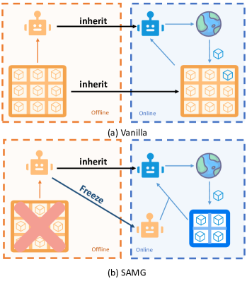
Figure 1: Compared with the vanilla O2O framework (a), the proposed SAMG (b) uses a frozen offline RL model with an adaptive distribution-aware model to achieve online fine-tuning with 100% online sample rates.

This compromise could result in several undesirable outcomes. Firstly, the quality of offline data is often heterogeneous, with portions of the data potentially being non-conducive to algorithmic improvement. Consequently, the effective information density within the offline dataset is relatively low. Secondly, the inefficiency in accessing online samples leads to a reduced capacity for exploiting new online knowledge, thereby complicating the process of model enhancement. This inefficiency contradicts the primary objective of the fine-tuning process, which aims to refine the offline model by integrating and absorbing novel information. Hence, existing O2O RL algorithms are hindered in both performance and efficiency.

To tackle the dilemma of low online sample utilization, it is constructive to directly leverage the offline critic, which is extracted from the offline dataset and represents an abstraction of the offline information. To this end, a novel online fine-tuning paradigm is proposed in this paper, named SAMG: State-Action-aware offline-to-online reinforcement learning with offline Model Guidance, which eliminates the burden of offline data and achieves 100% online sample utilization. SAMG freezes the offline critic which contains the offline cognition of the values given a state-action pair and offers guidance for online updating. SAMG combines the offline and online critic weighted by a state-action-aware coefficient to give a compound perspective of comprehension. The state-action-aware coefficient represents a class of functions that denotes the offline confidence of a given state-action pair. SAMG could be easily implemented based on Q-learning based RL algorithms, thus demonstrating strong applicability.

The main contributions of this paper are summarized as follows: (1) the compact offline information generated by the offline model is integrated into the fine-tuning process to guide the updating, (2) a novel class of state-action-adaptive functions is designed to provide distribution-aware weight. (3)Rigorous theoretical proofs demonstrate the convergence and estimation error. (4) by integrating SAMG into four Q-learning based algorithms, we evaluate the performance of four vanilla state-of-the-art offline RL and their corresponding SAMG-enhanced algorithms on the D4RL benchmark tasks, demonstrating the significant advantages of our algorithms.

Related works

Online RL with assistance of dataset. Expert level demonstrations are considered and combined with online data to accelerate online training process (Hester et al. 2018; Li et al. 2023; Nair et al. 2018; Rajeswaran et al. 2018; Vecerik et al. 2017), while other offline data is utilized to insert into the online replay buffer to supplement online learning process, without the requirement of being expert level, whose setting is called hybrid RL (Hester et al. 2018; Schaal 1996; Song et al. 2023). Auxiliary behavioral cloning losses with policy gradients are utilized to guide the updates and accelerate convergence (Kang, Jie, and Feng 2018; Zhu et al. 2019, 2018).

O2O RL. Large task-agnostic datasets are utilized to pre-train a model offline and feed for subsequent RL tasks online (Aytar et al. 2018; Baker et al. 2022; Fujimoto, Meger, and Precup 2019; Lifshitz et al. 2024; Yuan et al. 2024). Recent developments in model-based algorithms address high-dimensional problems and facilitate smooth, efficient adaptation to online samples (Lowrey et al. 2019; Mao et al. 2022; Rafailov et al. 2023).

A different category of work is to train the offline models with provided datasets and then fine-tune the pre-trained models online based on the offline datasets (Beeson and Montana 2022; Kostrikov, Nair, and Levine 2022; Lee et al. 2022; Lyu et al. 2022; Mark et al. 2022; Nair et al. 2020; Nakamoto et al. 2023; Wang et al. 2024; Wu et al. 2022). This line of work is based on offline algorithms (Kumar et al. 2020; Levine et al. 2020; Nair et al. 2020) and falls into the trap of buffer dependency. Most of these works inherit the large offline buffer while Cal-QL (Nakamoto et al. 2023) adopts the hybrid RL setting by evenly mixing online and offline samples (Song et al. 2023). Nevertheless, we demonstrate that they both reduce sample efficiency and struggle to handle changed environment dilemmas.

The pipeline of our work is most closely aligned with the approach proposed by Wang et al.(Wang et al. 2024), in which each paradigm is applicable to RL algorithms utilizing a Q-function. However, our specific implementation diverges significantly. Our method mainly differs from previous ones (Beeson and Montana 2022; Kostrikov, Nair, and Levine 2022; Lee et al. 2022; Lyu et al. 2022; Mark et al. 2022; Nair et al. 2020; Wu et al. 2022) that does not retain offline buffer and directly utilize the offline model for assistance instead.

Preliminaries

RL problem is defined as a sequential decision-making process, where a RL agent interacts with an environment in the form of Markov Decision Process (MDP), which is formulated as a tuple $\mathcal{M}=(\mathcal{S},\mathcal{A},P,r,\gamma,\tau)$. $\mathcal{S}$ represents the state space and $\mathcal{A}$ represents the action space. $P(s^{\prime}|s,a)$ denotes the unknown function of dynamics model and $r(s,a)$ denotes the unknown function of reward model limited by $|r(s,a)|\leq R_{max}$. $\gamma\in(0,1)$ denotes the discount factor for future reward and $\tau$ denotes the initial state distribution. The goal of RL is to acquire a policy $\pi(a|s)$ to maximize the cumulative discounted value function or state-value function, which are defined as $V^{\pi}(s)={\mathbb{E}_{a_{k}\sim\pi(s_{k})}[\sum_{k}\gamma^{k}r(s_{k},a_{k})|s_{0}=s]}$ and ${Q^{\pi}(s,a)={\mathbb{E}_{a_{k}\sim\pi(s_{k})}\left[\sum_{k}\gamma^{k}r(s_{k},a_{k})|s_{0}=s,a_{0}=a\right]}}$ respectively.

For actor-critic based RL algorithms, the training process alternates between policy evaluation and policy improvement. Policy evaluation phase maintains an estimated Q-function $Q_{\theta}(s,a)$ parameterized by $\theta$ and updates by applying the Bellman operator, $\mathcal{B}^{\pi}Q\doteq r+\gamma P^{\pi}Q$ (referred to as standard Bellman operator), where $P^{\pi_{\phi}}$ couples the dynamics function with the policy: $P^{\pi_{\phi}}Q(s,a)=\mathbb{E}_{s^{\prime}\sim P(s^{\prime}|s,a),a^{\prime}\sim\pi_{\phi}(a^{\prime}|s^{\prime})}[Q(s^{\prime},a^{\prime})]$. While policy improvement phase sustains a policy $\pi_{\phi}(a|s)$ parameterized by $\phi$ and updates the policy towards higher estimated values by the $Q_{\theta}(s,a)$.

SAMG: methodology

Our approach, Offline-Model-Guided and Distribution-Aware (SAMG) O2O RL, seeks to leverage the pre-trained offline model, rather than relying on the tedious offline data, to guide the online fine-tuning process. Therefore two critical questions arise:

• How can we accurately extract the information contained within the offline model?

• How can we adaptively incorporate the information into the online training process?

We introduce a model-guided technique alongside a state-action-aware weighting mechanism to resolve these issues.

Offline-model-guided technique

Offline-model-guided technique is designed to solve the problem 1. For an algorithm containing a state-action value function $Q_{(}s,a)$, which is approximated by some network $Q_{\theta}(s,a)$ parameterized by $\theta$. This function represents the quality given a specific state-action pair in the view of the offline dataset. So we can freeze and preserve this well-trained offline Q-network and query the offline opinion of the online state-action pairs. To combine the offline information with the online information, we integrate the frozen offline opinion with online Q-values with some weight. Formally, the following policy evaluation equation can be obtained:

$$Q(s,a)= r(s,a)+\gamma\left[(1-\alpha(s,a))Q(s^{\prime},a^{\prime})\right.$$ (1)

$$+\left.{\color[rgb]{0,0,1}{\alpha(s,a)Q^{off}(s^{\prime},a^{\prime})}}\right].$$

where the Q-network and $\alpha\in(0,1)$ denote a function class that gives a state-action-adaptive weight and can be implemented with any reasonable form. Novel parts that differ from the standard Bellman equation is marked in blue.

Distribution-aware weight

The function class $\alpha(s,a)$ provides the distribution-aware weights to solve the problem 2. Intuitively, we tend to assign high weights to samples within the offline distribution because we have prior comprehension of these samples and the judgment of the offline model is reliable. As for samples distant from the offline distribution, which can be treated as OOD samples, we have limited knowledge about them and tend to assign low weights to them. Any structure that satisfies this requirement could be treated as an instantiation of SAMG.

In this paper, the conditional variational auto-encoder (C-VAE)  (Kingma et al. 2014) is mainly utilized to infer the offline confidence of online samples, which is broadly used in offline algorithms to represent the behavior policy (Fujimoto, Meger, and Precup 2019; Kumar et al. 2019; Xu, Zhan, and Zhu 2022), and an embedding network (Badia et al. 2019) is briefly introduced as well. Previous works leverage the C-VAE structure to construct the divergence error, which is distant from our setting. While Xu (Xu, Zhan, and Zhu 2022) adopts a similar setting to our work, their C-VAE structure is state-conditional. We find such structure might suffer from posterior collapse (Lucas et al. 2019; Wang, Blei, and Cunningham 2021) in certain environments, as illustrated in Appendix B.1.1.

Posterior collapse implies that the encoder completely fails and the KL-divergence term vanishes to zero for any input. Thus, the decoder structure actually takes noise as input and reconstructs a sample all by itself. This phenomenon is extremely detrimental in RL setting because the output of the encoder is needed for the distribution-aware weight but it now fails to operate.

To overcome this challenge, the C-VAE structure is updated that the encoder takes the state-action pairs as input to meet the state-action-adaptive requirement and the decoder reconstructs from the latent layer conditioned on state-action pairs (similar to the role of RL environments). We also utilize the KL-annealing technique (Bowman et al. 2015) in some environments, detailed in Appendix B.1.2. Through this approach, our state-action-aware C-VAE structure could better resist the posterior collapse. Formally, SAMG adopts the following evidence lower bound (ELBO) on the offline dataset to get the state-action-aware C-VAE:

$$\max\limits_{\psi_{1},\psi_{2}}\mathbb{E}_{z\sim\text{Enc}_{\psi_{1}}} \left[\log\text{Dnc}_{\psi_{2}}(s^{\prime}|z,s,a)\right]$$ (2)

$$-\beta D_{KL}\left[{\text{Enc}_{\psi_{1}}(z|s,a)}||{\text{Dnc}_{\psi_{2}}(z)}\right]$$

where $\text{Enc}_{\psi_{1}}(z|s,a)$ and $\text{Dnc}_{\psi_{2}}(s^{\prime}|z,s,a)$ represent the encoder structure and decoder structure respectively; $\text{Dnc}_{\psi_{2}}(z)$ denotes the prior distribution of the encoder; and $D_{KL}\left[p||q\right]$ denotes the Kullback-Leibler divergence. The former error term denotes the reconstruction loss of the encoder and the latter one denotes the Kullback-Leibler divergence between encoder distribution and the prior distribution of $z$.

After fitting the C-VAE network, a well-converged estimator can be obtained which encodes the state-action pair to a nearly standard normal distribution, i.e., the output mean value is around 0 and the output standard value is approximately 1, as shown in Appendix B.1.3. However, it is impractical to directly utilize the information of the latent layer because the latent layer is sampled from an approximate standard normal distribution and the sampling randomness completely overwhelms the latent layer information.

Therefore, we collect the output mean and standard values of all the offline data and fit the mean and standard values with two different normal distributions, denoted as $\mathcal{N}_{M}(a_{mean},b_{mean}),\mathcal{N}_{S}(a_{std},b_{std})$. Then the usual range of the mean and standard values of the offline data can be obtained and employed to judge the offline confidence of online samples based on these two normal distributions.

Formally, the weight value with the mean probability of the latent layer of online samples $(a,b)$ falling within a distance less than $|a-a_{mean}|$ for mean output and $|b-b_{mean}|$ for standard output. The cumulative distribution function $F_{X}(x)$ is leveraged to get the probability of an online sample aligning with the offline distribution. We find that the estimation of the standard value sometimes has measurable errors. Therefore, we only utilize the mean value in practice. Moreover, in cases where the sample diverges notably from the offline distribution, the information about the sample is unknown so the probability is manually set to be 0, with a hyperparameter $p_{om}$ introduced. The eventual equation to calculate the probability $p_{o}$ of a given sample $(a,b)$ is illustrated below:

$$\begin{split}\left\{\begin{aligned} &|F_{M}(a)-F_{M}(2a_{mean}-a)|,&if\ p_{o}(s,a)\geq p_{om}\\ &0,&if\ p_{o}(s,a)<p_{om}\end{aligned}\right.\end{split}$$ (3)

By integrating the C-VAE form distribution-aware weights into Equation 1, the following practical updating expression can be obtained:

$$Q(s,a)= r(s,a)+\gamma\left[(1-p_{o}(s,a))Q(s^{\prime},a^{\prime})\right.$$ (4)

$$+\left.{\color[rgb]{0,0,1}{p_{o}(s,a)Q^{off}(s^{\prime},a^{\prime})}}\right].$$

Comprehension of distribution-aware weight. The distribution-aware weight module actually attempts to depict the characteristics of the complex distribution represented by the offline dataset. Considering the high-dimensional and continuous property of the state-action data, it is challenging to directly extract the probability characteristics from the state-action pair. Therefore, it is required to perform dimension reduction of the distribution of the offline dataset, i.e., the complex distribution is simplified to be a normal distribution.

Analysis of SAMG

Intuitive analysis of SAMG

Intrinsic reward form of SAMG. Equation 4 can be derived as below:

$$Q(s,a)= \left[r(s,a)+\gamma p_{o}(s,a)(Q^{off}(s^{\prime},a^{\prime})-Q(s^{\prime},a^{\prime}))\right]$$ (5)

$$+\gamma Q(s^{\prime},a^{\prime}).$$

Equation 5 indicates that the induced offline information could be treated in the form of intrinsic reward. The intrinsic reward is composed of the difference between offline and online state-action value factored by the distribution-aware weight. The intrinsic reward term can be analyzed in two possible situations. If the state-action pair is within the offline distribution where the offline Q-value is reasonably trained and the distribution-aware wight $\alpha$ is notable, then this term suggests that the higher the offline Q-value, the higher the reward. Hence, this intrinsic reward term encourages state-action pairs with higher performance. However, if the state-action pair falls outside the offline distribution where the offline Q-value may be mis-estimated, the wight $p_{o}$ is paltry or even set to zero according to Equation 3 and this term is insignificant. Therefore, SAMG could properly utilize the knowledge of the offline model, which is exactly what we expect.

Bellman form of SAMG. Furthermore, Equation 1 can be derived to the following equation by applying the bellman operator:

$$Q(s,a)=(1-p_{o}(s,a))\mathcal{B}^{\pi}Q+p_{o}(s,a)\mathcal{B}^{\pi}Q^{off}.$$ (6)

where $\mathcal{B}^{\pi}Q$ is the standard bellman equation and $\mathcal{B}^{\pi}Q^{off}=r(s,a)+\gamma Q^{off}(s^{\prime},a^{\prime})$ is the offline bellman equation of the fixed offline state action function.

It can be obtained that our method actually incorporates the standard Bellman equation with the offline Bellman equation by weight $p_{o}(s,a)$ and this paradigm just combines the offline opinion with the online opinion weighted by the sample property. More importantly, SAMG reverts to the vanilla algorithm when dealing with OOD samples. This allows SAMG to take full advantage of the conservative settings of the vanilla algorithm for OOD samples. Therefore, SAMG does not induce over-estimation on OOD samples even though SAMG gets rid of the offline dataset. Consequently, SAMG effectively utilizes the vanilla wisdom for handling OOD samples.

Theoretical analysis of SAMG

In this section, the temporal difference algorithm (Sutton 1988; Haarnoja et al. 2018) is adopted and Equation 4 is proven to still converge to the same optimalily, even with an extra term induced in the tabular setting. For the theoretical tools, SAMG gets rid of the offline dataset and therefore diverges from the hybrid realm of Song et al. (Song et al. 2023) and offline RL scope limited by the dataset, but aligns completely with traditional online RL algorithms (T. Jaakkola and Singh 1994; Thomas 2014; Haarnoja et al. 2018).

Contraction property. Since the standard Bellman operator is broken and a term that could be considered as offline Bellman operator is introduced, we first proof that SAMG still satisfies the contraction property (Keeler and Meir 1969). The contraction property forms the basis for the necessity of convergence of the iterative RL algorithms. The related theorem and detailed proof can be found in Appendix A.1.

Convergence optimality and estimation error. Formally, the estimated state-value function at time-step $k$ for any given pair $(s,a)$ is denote by $Q_{k}(s,a)$ and the iterative TD updating form of Equation 4 is shown as below:

$$\begin{split}&Q_{k+1}(s,a)-Q_{k}(s,a)\\ =&\alpha_{k}(s,a)\left[Q_{k}(s,a)-\left(r_{k+1}+\gamma Q_{k}(s_{k+1},a_{k+1})\right)\right]-\\ &\alpha_{k}(s,a)\gamma p(s,a)\left(Q^{off}(s_{k+1},a_{k+1})-Q_{k}(s_{k+1},a_{k+1})\right)\end{split}$$ (7)

To prove the optimality of SAMG, the Dvoretzky’s Theorem (Dvoretzky 1959) is introduced.

Lemma 1 (Dvoretzky’s Theorem).

Consider a finite set $\mathcal{S}$ of real numbers. For the stochastic process:

$$\begin{split}\Delta_{k+1}(s)=\left(1-\alpha_{k}(s)\right)\Delta_{k}(s)+\beta_{k}(s)\eta_{k}(s).\end{split}$$

It holds that $\Delta_{k}(s)$ convergences to zero almost surely for every $s\in\mathcal{S}$ if the following conditions are satisfied for $s\in\mathcal{S}$:

(a) $\sum_{k}\alpha_{k}(s)=\infty,$ $\sum_{k}\alpha_{k}^{2}(s)<\infty$, $\sum\limits_{k}\beta_{k}^{2}(s)<\infty$, $\mathbb{E}[\beta_{k}(s)|\mathcal{H}_{k}]\leq\mathbb{E}[\alpha_{k}(s)|\mathcal{H}_{k}]$ uniformly almost surely;

(b) $\big{\|}{\mathbb{E}[\eta_{k}(s)|\mathcal{H}_{k}]}\big{\|}_{\infty}\leq\gamma\big{\|}\Delta_{k}\big{\|}_{\infty}$, with $\gamma\in(0,1)$;

(c) $var\left[\eta_{k}(s)|\mathcal{H}_{k}\right]\leq C\left(1+\big{\|}\Delta_{k}(s)\big{\|}_{\infty}\right)^{2}$, with $C$ a constant. Here, $\mathcal{H}_{k}=\{\Delta_{k},\Delta_{k-1},\cdots,\eta_{k-1},\cdots,\alpha_{k-1}$, $\cdots,\beta_{k-1},\cdots\}$ denotes the historical information. The term $\|\cdot\|_{\infty}$ represents the maximum norm.

The incremental form of SAMG is derived and proven to satisfy these conditions and the following optimality conclusion is obtained. Details refer to Appendix A.2.

Theorem 1 (Optimality of SAMG).

Given a policy $\pi$, by the TD updating paradigm, $Q_{k}(s,a)$ of SAMG converges almost surely to $Q_{\pi}(s,a)$ as $k\to\infty$ for all $s\in\mathcal{S}$ and $a\in\mathcal{A}$ if $\sum_{k}\alpha_{k}(s,a)=\infty$ and $\sum_{k}\alpha_{k}^{2}(s,a)<\infty$ for all $s\in\mathcal{S}$ and $a\in\mathcal{A}$.

Moreover, the following theorem on convergence estimation error is obtained during the derivation of the second condition.

Theorem 2 (Estimation error of SAMG).

The error term $\eta_{k}(s,a)$ is limited by,

$$\big{\|}\mathbb{E}[\eta_{k}(s,a)]\big{\|}_{\infty}$$

$$\leq \left\{\begin{aligned} &\begin{aligned} &\gamma\left(1-p(s_{k},a_{k})\right)\big{\|}\Delta_{k}(s,a)\big{\|}_{\infty}+\\ &\gamma\gamma_{\mathcal{F}}p(s_{k},a_{k})\mathcal{O}(\big{\|}\Delta_{k}(s,a)\big{\|}_{\infty}),\end{aligned}&p(s,a)\geq p_{m}\\ &\gamma\big{\|}\Delta_{k}(s,a)\big{\|}_{\infty},&p(s,a)<p_{m}\end{aligned}\right.$$ (8)

where $0<\gamma_{\mathcal{F}}<1$ denotes the convergence coefficient of offline algorithm class $\mathcal{F}$ and $\mathcal{O}(\big{\|}\Delta_{k}(s,a)\big{\|}_{\infty})$ denotes the high-order infinitesimal of $\big{\|}\Delta_{k}(s,a)\big{\|}_{\infty}$.

Theorem 2 indicates that SAMG converges faster than standard RL algorithms on samples within the distribution of offline datasets, illustrating the distribution-aware advantage of SAMG, and at least the same speed on OOD samples. For samples within the distribution, the convergence speed depends on the offline confidence implied by $p(s,a)$, i.e., a higher $p(s,a)$ indicates a higher degree of offline-ness, corresponding to a smaller error term constrained by the term $(1-p(s,a))$ and ensuring faster convergence. For the OOD samples, the algorithm degenerates into the traditional algorithm because $p(s,a)$ is set to zero as stated in Equation 3. The theoretical result is highly consistent with the analysis of the expected performance as shown in Section Intuitive analysis of SAMG and demonstrates evident performance enhancement. Furthermore, the theoretical result indicates that the extent of algorithm improvement is determined by the sample coverage rate of the offline dataset. Specifically, the algorithm’s performance is enhanced with more comprehensive sample coverage, whereas its improvement is constrained in scenarios with limited sample diversity.

Experimental Results

Our experimental evaluation focuses on the performance of SAMG after fine-tuning based on four state-of-the-art algorithms on a wide range of offline benchmark tasks containing D4RL (Fu et al. 2020). All experiments are conducted with compute source detailed in Appendix D.

Baselines. (i) SAMG algorithms, the SAMG paradigm is constructed on a variety of state-of-the-art O2O RL algorithms, including CQL (Kumar et al. 2020), AWAC (Nair et al. 2020), IQL (Kostrikov, Nair, and Levine 2022)and Cal_QL (Nakamoto et al. 2023). All algorithms are implemented based on library CORL (Tarasov et al. 2024) with implementation details in Appendix C.1 and C.2. (ii) O2O RL algorithms, we implement the aforementioned O2O RL algorithms (CQL, AWAC, IQL and Cal_QL). We also implement TD3+BC (Fujimoto and Gu 2021) and SPOT (Wu et al. 2022). (iii) Behavior Cloning (BC), we implement Behavior cloning algorithms based on (Chen et al. 2020).

Benchmark tasks. We evaluate our algorithm and the baselines across multiple benchmark tasks: (1) The D4RL locomotion tasks (Fu et al. 2020), including three different kinds of environments (Halfcheetah, Hopper, Walker2d) where different robots are manipulated to complete different tasks on three different levels of datasets. (2) The AntMaze tasks that an "Ant" robot is controlled to explore and navigate to random goal locations in six levels of environments, as detailed in Appendix C.3.

Table 1: Performance comparison. The D4RL normalized score (Fu et al. 2020) is evaluated of standard base algorithms (including CQL (Kumar et al. 2020), IQL (Kostrikov, Nair, and Levine 2022), AWAC (Nair et al. 2020) and Cal_QL (Nakamoto et al. 2023), denoted as "Vanilla") in comparison to the base algorithms augmented with SAMG (referred to as "Ours"), as well as three baselines (BC, TD3BC (Chen et al. 2020), SPOT (Wu et al. 2022)). The superior scores are highlighted in blue.

Dataset1	CQL		AWAC		IQL		Cal-QL		BC	TD3BC	SPOT
	Vanilla	Ours	Vanilla	Ours	Vanilla	Ours	Vanilla	Ours
Hopper-mr	100.9(0.1)	103.7(1.3)	101.7(2.5)	110.0(1.2)	99.6(1.3)	101.8(0.9)	103.4(0.4)	108.7(0.1)	59.9 (2.2)	99.4(1.3)	99.2(4.6)
Hopper-m	72.9(6.9)	93.6(4.8)	102.3(2.4)	104.1(10.0)	70.9(3.7)	74.1(5.3)	88.6(7.6)	112.9(2.5)	58.1(1.7)	66.4(1.6)	87.1(5.3)
Hopper-me	111.7(0.5)	113.0(0.3)	112.0(1.8)	112.8(7.2)	85.1(28.7)	95.7(6.1)	102.1(0.2)	112.3(1.5)	83.4(14.6)	97.4(9.1)	97.8(6.5)
Antmaze-u	98.0(2.0)	99.0(1.0)	70.0(40.4)	87.0(13.2)	94.0(1.0)	95.6(2.0)	99.8(0.4)	97.0(1.1)	54.2(3.7)	72.4(28.5)	99.5(0.5)
Antmaze-ud	95.0(1.7)	93.0(3.2)	16.0(35.3)	65.0(7.1)	75.6(20.4)	94.0(4.6)	95.4(3.0)	96.4(1.8)	46.3(3.8)	46.2(14.5)	92.5(3.7)
Antmaze-md	88.0(7.9)	97.0(1.0)	0.0(0.0)	0.0(0.0)	90.6(3.8)	96.5(1.9)	97.0(2.8)	96.0(2.1)	0.0(0.0)	0.2(0.2)	92.0(1.5)
Antmaze-mp	90.0(4.6)	96.2(4.0)	0.0(0.0)	0.0(0.0)	92.0(3.8)	94.8(1.6)	98.0(1.2)	96.0(1.6)	0.8(0.6)	0.3(0.3)	97.2(1.7)
Antmaze-ld	71.6(1.4)	70.8(2.8)	0.0(0.0)	0.0(0.0)	67.4(4.2)	81.5(7.9)	85.6(9.4)	87.2(4.7)	0.0(0.0)	0.0(0.0)	85.5(3.2)
Antmaze-lp	61.2(0.7)	75.0(2.1)	0.0(0.0)	0.0(0.0)	68.6(6.2)	74.8(8.4)	91.0(4.6)	90.0(1.2)	0.0(0.0)	0.0(0.0)	81.0(16.8)

• mr: medium-replay, m: medium, l: large, me: medium-expert, d: diverse, p: play.

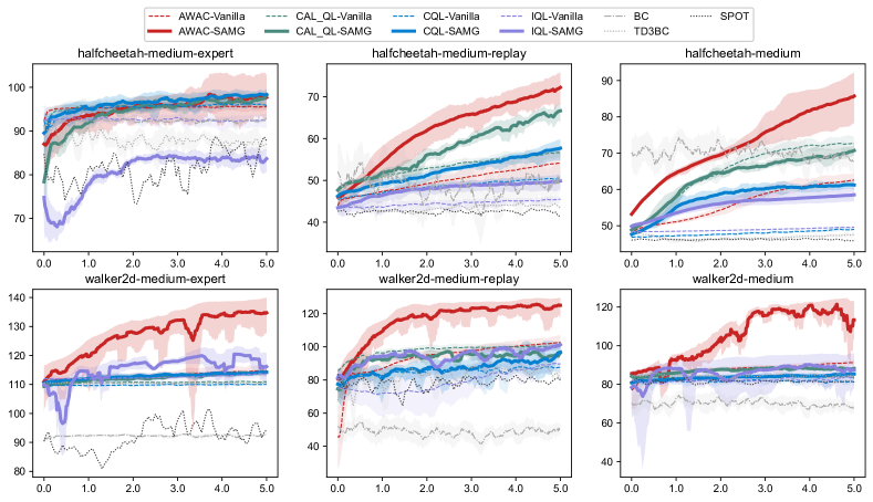
Figure 2: Algorithm performance in the online fine-tuning phase after offline pretraining. This figure plots the performance of SAMG and the other baselines during the online fine-tuning phase on part of the benchmarks (halfcheetah and walker2d). SAMG outperforms or at least matches the previous methods. The results are averaged on 5 seeds.

Empirical results

We first represent the normalized scores of the vanilla algorithms with and without SAMG integrated. The normalized scores through training on Walker2d and Halfcheetah environments are shown in Figure 2. Constrained by the space, we present the final normalized scores of the other environments (Hopper and Antmaze) in Table 1.

As shown in the Figure 2 and the Table 1, SAMG consistently outperforms the vanilla algorithms in the majority of environments, illustrating the superiority of our paradigm. Moreover, it is interesting to note that SAMG exhibits the best performance on the simple algorithm AWAC. SAMG still yields significant improvements on the other algorithms with more complex settings, but not as significant as AWAC. The reason for this counter-intuitive phenomenon is discussed in Appendix C.4., which just illustrates the effectiveness of SAMG. We present the cumulative regret on environment Antmaze in appendix C.5., further demonstrating the outstanding online sample efficicy of SAMG.

Although SAMG performs well in most environments, it is still worthwhile to notice SAMG may occasionally behave unsatisfactory(e.g., IQL-SAMG on Halfcheetah-medium-expert environment). We discuss in the Appendix C.6. that this exception is caused by the special property of the environment and IQL, rather than the defect of SAMG. We notice that the AWAC algorithm performs poorly in the Antmaze environment which also results in SAMG struggling to initiate. This is because AWAC algorithm is relatively simple and not competent for the complex environment of Antmaze, it is an inherent limitation of the AWAC algorithm, rather than an issue with SAMG. In summary, SAMG demonstrates performance increase by average 10.01% across four vanilla algorithms (for a total examined 15 tasks), indicating its robustness and versatility.

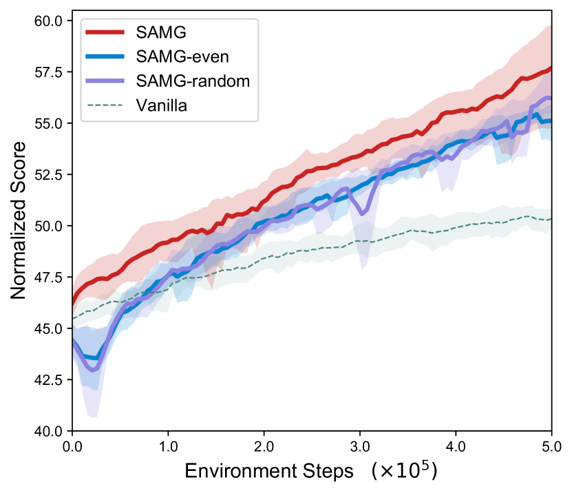
Figure 3: Ablation study for the distribution-aware weight.

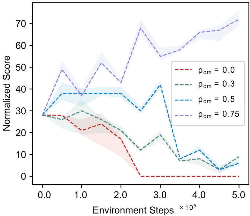
Figure 4: Sensitivity test for the threshold $p_{om}$.

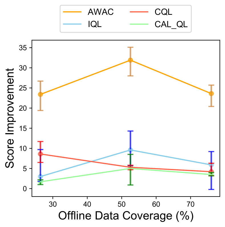
Figure 5: Average improvement of the normalized score over the offline data coverage.

Ablation study of distribution-aware weight

The state-action-aware weight $\alpha(s,a)$ provides an estimate of the offline degree given a $(s,a)$ pair and is instantiated as $p_{o}$ of the C-VAE model. To demonstrate the impact of the state-action-aware weight, we compare several different architectures on the environment Halfcheetah-medium with CQL-SAMG, including: (i) SAMG, (ii) 1/2 for online and 1/2 for offline (denoted as SAMG-even), (iii) random probability (generate random probability, denoted as SAMG-random), (iv) the vanilla RL algorithms.

The casual selection of C-VAE decreases the algorithm performance during the initial training phase which is even notably inferior to the vanilla algorithms and can never exceed the SAMG performance (Figure 5). Moreover, SAMG with casual C-VAE catches up with and surpasses the performance of the vanilla algorithms, which highlights the advantage of SAMG paradigm. SAMG manages to eliminate the influence of offline datasets, so once the algorithm adapts to the new environment, the algorithm is able to explore the environment and achieve higher scores. SAMG improves over the SAMG-even and vanilla algorithms by 15.3% and 5.2%, respectively. Furthermore, the state-action-aware weight represents a class of functions, as stated in Section SAMG: methodology. Given that $\alpha$ represents a class of function, we provide some other possible implementation techniques, as detailed in the Appendix A.2.

Sensitivity analysis of threshold $p_{om}$

It is a crucial hyperparameter that $p_{om}$ holds the lower threshold of OOD samples. We evaluate the sensitivity of $p_{om}$ on environment Antmaze-large-diverse with IQL-SAMG across a range of numbers, including 0, 0.3, 0.5, 0.75 (normal value). The results are shown in Figure 5. We find that $p_{om}$ is more sensitive in more complex environments, like Antmaze. Inappropriate selection of $p_{om}$ may lead to a decline in algorithm performance, or even complete divergence, thus highlighting the importance of $p_{om}$.

Does SAMG rely on offline data coverage?

This part aims to evaluate the relationship between algorithm performance improvement and the coverage rate of the offline dataset to showcase the effect. To model the data coverage of the offline dataset, We apply t-SNE (Van der Maaten and Hinton 2008) to perform dimensionality reduction, then cluster with t-SNE information on all levels of datasets of a given environment, as detailed in Appendix C.7.

The results illustrate that SAMG indeed correlates with the sample coverage rate (See Figure 5, where The left represents the medium-replay level, the middle represents the medium level and the right represents the medium-expert level of the dataset). Middle sample coverage rate yields greater performance improvement for SAMG, while higher or lower coverage rates lead to less significant performance improvements. This is because that lower coverage rates induce a narrow distribution of the offline dataset, resulting in limited information and accuracy of the offline model. Conversely, higher coverage rates often contribute to satisfaction with the offline model, hence further improvement is limited. However, SAMG consistently achieves improvements over vanilla algorithms and moderate sample coverage rates are common in practical applications, highlighting the superiority of SAMG.

Conclusion, limitation and future work

In this paper, a novel paradigm named SAMG is proposed to eliminate the tedious usage of offline data and leverage the pre-trained offline model instead, thereby ensuring 100% online sample utilization and better fine-tuning performance. SAMG freezes the offline critic and combines online and offline critics with a state-action-aware coefficient. The state-action-aware coefficient models the complex distribution of the offline dataset and provides the probability of a given state-action sample deviating from the offline distribution. Theoretical analysis proves the convergence optimality and lower estimation error. Experimental results demonstrate the superiority of SAMG over vanilla baselines. However, it can be noticed that performance improvement of SAMG is limited if the offline dataset distribution is extremely narrow. This limitation could potentially be mitigated by designing specific update strategies for OOD samples, which serves as an interesting direction for future work.

Reproducibility Checklist

1. This paper

   • Includes a conceptual outline and/or pseudocode description of AI methods introduced (yes)

   • Clearly delineates statements that are opinions, hypothesis, and speculation from objective facts and results (yes)

   • Provides well marked pedagogical references for less-familiare readers to gain background necessary to replicate the paper (yes)

2. Theoretical contributions

   Does this paper make theoretical contributions? (yes)

   • All assumptions and restrictions are stated clearly and formally. (yes)

   • All novel claims are stated formally (e.g., in theorem statements). (yes)

   • Proofs of all novel claims are included. (yes)

   • Proof sketches or intuitions are given for complex and/or novel results. (yes)

   • Appropriate citations to theoretical tools used are given. (yes)

   • All theoretical claims are demonstrated empirically to hold. (yes)

   • All experimental code used to eliminate or disprove claims is included. (yes)

3. Reliance on datasets

   • A motivation is given for why the experiments are conducted on the selected datasets (yes)

   • All novel datasets introduced in this paper are included in a data appendix. (NA)

   • All novel datasets introduced in this paper will be made publicly available upon publication of the paper with a license that allows free usage for research purposes. (NA)

   • All datasets drawn from the existing literature (potentially including authors’ own previously published work) are accompanied by appropriate citations. (yes)

   • All datasets drawn from the existing literature (potentially including authors’ own previously published work) are publicly available. (yes)

   • All datasets that are not publicly available are described in detail, with explanation why publicly available alternatives are not scientifically satisficing. (NA)

4. Computational experiments

   • Any code required for pre-processing data is included in the appendix. (yes).

   • All source code required for conducting and analyzing the experiments is included in a code appendix. (yes)

   • All source code required for conducting and analyzing the experiments will be made publicly available upon publication of the paper with a license that allows free usage for research purposes. (yes)

   • All source code implementing new methods have comments detailing the implementation, with references to the paper where each step comes from (yes)

   • If an algorithm depends on randomness, then the method used for setting seeds is described in a way sufficient to allow replication of results. (yes)

   • This paper specifies the computing infrastructure used for running experiments (hardware and software), including GPU/CPU models; amount of memory; operating system; names and versions of relevant software libraries and frameworks. (yes)

   • This paper formally describes evaluation metrics used and explains the motivation for choosing these metrics. (yes/partial/no)

   • This paper states the number of algorithm runs used to compute each reported result. (yes)

   • Analysis of experiments goes beyond single-dimensional summaries of performance (e.g., average; median) to include measures of variation, confidence, or other distributional information. (yes)

   • The significance of any improvement or decrease in performance is judged using appropriate statistical tests (e.g., Wilcoxon signed-rank). (yes)

   • This paper lists all final (hyper-)parameters used for each model/algorithm in the paper’s experiments. (yes)

   • This paper states the number and range of values tried per (hyper-) parameter during development of the paper, along with the criterion used for selecting the final parameter setting. (yes)

Appendices

Appendix A A. Theoretical analysis

A.1. Contraction property

Our algorithm actually breaks the typical Bellman Equation of the RL algorithm denoted as $Q=\max\limits_{\pi\in\Pi}\mathcal{B}^{\pi}=\max\limits_{\pi\in\Pi}(r_{\pi}+\gamma P_{\pi}Q)$. Instead we promote Equation 6. In order to prove the convergence of the updating equation, we introduce the contraction mapping theorem which is widely used to prove the convergence optimality of RL algorithm.

Theorem 3 (Contraction mapping theorem).

For an equation that has the form of $x=f(x)$ where $x$ and $f(x)$ are real vectors, if $f$ is a contraction mapping which means that $\|f(x_{1})-f(x_{2})\|\leq\gamma\|x_{1}-x_{2}\|(0<\gamma<1)$, then the following properties hold.

Existence: There exists a fixed point $x^{*}$ that satisfies $f(x^{*})=x^{*}$.

Uniqueness: The fixed point $x^{*}$ is unique.

Algorithm: Given any initial state $x_{0}$, consider the iterative process: $x_{k+1}=f(x_{k})$, where $k=0,1,2,...$. Then $x_{k}$ convergences to $x^{*}$ as $k\to\infty$ at an exponential convergence rate.

We just need to prove that this equation satisfies the contraction property of theorem  3 and naturally we can ensure the convergence of the algorithm.

Take the right hand of equation  (6) as function $f(Q)$ and consider any two vectors $Q_{1},Q_{2}\in\mathbb{R}^{\mathcal{S}}$, and suppose that $\pi_{1}^{*}\doteq\mathop{\arg\max}\limits_{\pi}(r_{\pi}+\gamma P_{\pi}Q_{1})$, $\pi_{2}^{*}\doteq\mathop{\arg\max}\limits_{\pi}(r_{\pi}+\gamma P_{\pi}Q_{2})$. Then,

$$\begin{split}f(Q_{1})=&\max\limits_{\pi}\left[(1-p(s,a))\mathcal{B}^{\pi}Q_{1}+p(s,a)\mathcal{B}^{\pi}Q^{off})\right]\\ =&(1-p(s,a))\mathcal{B}^{\pi_{1}^{*}}Q_{1}+p(s,a)\mathcal{B}^{\pi_{1}^{*}}Q^{off}\\ \geq&(1-p(s,a))\mathcal{B}^{\pi_{2}^{*}}Q_{1}+p(s,a)\mathcal{B}^{\pi_{2}^{*}}Q^{off},\end{split}$$ (9)

and similarly:

$$\begin{split}f(Q_{2})\geq(1-p(s,a))\mathcal{B}^{\pi_{1}^{*}}Q_{2}+p(s,a)\mathcal{B}^{\pi_{1}^{*}}Q^{off}.\end{split}$$ (10)

To simplify the derivation process, we use $p^{\pi}$ to represent $p(s,\pi(a|s))$ considering that values of $p$ function class are determined by the policy $\pi$ of any given state. As a result,

$$\begin{split}&f(Q_{1})-f(Q_{2})\\ =&(1-p^{\pi_{1}^{*}})\mathcal{B}^{\pi_{1}^{*}}Q_{1}+p^{\pi_{1}^{*}}\mathcal{B}^{\pi_{1}^{*}}Q^{off}\\ &-\left[(1-p^{\pi_{2}^{*}})\mathcal{B}^{\pi_{2}^{*}}Q_{2}+p^{\pi_{2}^{*}}\mathcal{B}^{\pi_{2}^{*}}Q^{off}\right]\\ \leq&(1-p^{\pi_{1}^{*}})\mathcal{B}^{\pi_{1}^{*}}Q_{1}+p^{\pi_{1}^{*}}\mathcal{B}^{\pi_{1}^{*}}Q^{off}-\\ &\left[(1-p^{\pi_{1}^{*}})\mathcal{B}^{\pi_{1}^{*}}Q_{2}+p^{\pi_{1}^{*}}\mathcal{B}^{\pi_{1}^{*}}Q^{off}\right]\\ =&(1-p^{\pi_{1}^{*}})(\mathcal{B}^{\pi_{1}^{*}}Q_{1}-\mathcal{B}^{\pi_{1}^{*}}Q_{2})\\ =&\gamma(1-p^{\pi_{1}^{*}})P^{\pi_{1}^{*}}(Q_{1}-Q_{2})\\ \leq&\gamma P^{\pi_{1}^{*}}(Q_{1}-Q_{2}).\end{split}$$ (11)

We can see that the result reduces to that of the normal Bellman equation and therefore, the following derivation is omitted. As a result, we get,

$$\begin{split}\|f(Q_{1})-f(Q_{2})\|_{\infty}\leq\gamma\|Q_{1}-Q_{2}\|_{\infty},\end{split}$$ (12)

which concludes the proof of the contraction property of $f(Q)$.

A.2. Convergence optimality

We consider a tabular setting for simplicity. We first write down the iterative form of Equation 4 as below:

if $s=s_{k},a=a_{k}$,

$$\begin{split}&Q_{k+1}(s,a)=Q_{k}(s,a)\\ &-\alpha_{k}(s,a)\left[Q_{k}(s,a)-\left(r_{k+1}+\gamma Q_{k}(s_{k+1},a_{k+1})\right)\right]\\ &-\alpha_{k}(s,a)\gamma p(s,a)\left(Q^{off}(s_{k+1},a_{k+1})-Q_{k}(s_{k+1},a_{k+1})\right).\end{split},$$ (13)

else,

$$\begin{split}Q_{k+1}(s,a)=Q_{k}(s,a).\end{split}$$ (14)

The error of estimation is defined as:

$$\begin{split}\Delta_{k}(s,a)\doteq Q_{k}(s,a)-Q_{\pi}(s,a).\end{split}$$ (15)

where $Q_{\pi}(s,a)$ is the state action value s under policy $\pi$. Deducting $Q_{\pi}(s,a)$ from both sides of 7 gets:

$$\begin{split}\Delta_{k+1}(s,a)=&\left(1-\alpha_{k}(s,a)\right)\Delta_{k}(s,a)\\ &+\alpha_{k}(s,a)\eta_{k}(s,a),\quad s=s_{k},a=a_{k}.\end{split}$$ (16)

where

$$\begin{split}&\eta_{k}(s,a)\\ =&\left[r_{k+1}+\gamma Q_{k}(s_{k+1},a_{k+1})-Q_{\pi}(s,a)\right]\\ &+\gamma p(s,a)\left(Q^{off}(s_{k+1},a_{k+1})-Q_{k}(s_{k+1},a_{k+1})\right)\\ =&\left[r_{k+1}+\gamma Q_{k}(s_{k+1},a_{k+1})-Q_{\pi}(s,a)\right]\\ &+\gamma p(s,a)\left\{\left[Q^{off}(s_{k+1},a_{k+1})-Q_{\pi}(s_{k+1},a_{k+1})\right]\right.\\ &\left.+\left[Q_{\pi}(s_{k+1},a_{k+1})-Q_{k}(s_{k+1},a_{k+1})\right]\right\}\\ =&\underbrace{\left[r_{k+1}+\gamma Q_{k}(s_{k+1},a_{k+1})-Q_{\pi}(s,a)\right]}_{\Gamma_{1}}\\ &-\underbrace{\gamma p(s,a)\left(Q_{k}(s_{k+1},a_{k+1})-Q_{\pi}(s_{k+1},a_{k+1})\right)}_{\Gamma_{2}}\\ &+\underbrace{\gamma p(s,a)\left(Q^{off}(s_{k+1},a_{k+1})-Q_{\pi}(s_{k+1},a_{k+1})\right)}_{\Gamma_{3}}.\end{split}$$ (17)

Similarly, deducting $Q_{\pi}(s,a)$ from both side of Equation 14 gets:

$$\begin{split}\Delta_{k+1}(s,a)=&\left(1-\alpha_{k}(s,a)\right)\Delta_{k}(s,a)\\ &+\alpha_{k}(s,a)\eta_{k}(s,a),\quad s\neq s_{k}\ or\ a\neq a_{k}.\end{split}$$

this expression is the same as 16 except that $\alpha_{k}(s,a)$ and $\eta_{k}(s,a)$ is zero. Therefore we observe the following unified expression:

$$\begin{split}\Delta_{k+1}(s,a)=\left(1-\alpha_{k}(s,a)\right)\Delta_{k}(s,a)+\alpha_{k}(s,a)\eta_{k}(s,a).\end{split}$$

To further analyze the convergence property, we introduce Dvoretzky’s theorem [T. Jaakkola and Singh, 1994]:

Theorem 4 (Dvoretzky’s Throrem).

Consider a finite set $\mathcal{S}$ of real numbers. For the stochastic process:

$$\begin{split}\Delta_{k+1}(s)=\left(1-\alpha_{k}(s)\right)\Delta_{k}(s)+\beta_{k}(s)\eta_{k}(s).\end{split}$$

it holds that $\Delta_{k}(s)$ convergences to zero almost surely for every $s\in\mathcal{S}$ if the following conditions are satisfied for $s\in\mathcal{S}$:

• $\sum_{k}\alpha_{k}(s)=\infty,\sum_{k}\alpha_{k}^{2}(s)<\infty,$ $\sum\limits_{k}\beta_{k}^{2}(s)<\infty$, $\mathbb{E}[\beta_{k}(s)|\mathcal{H}_{k}]\leq\mathbb{E}[\alpha_{k}(s)|\mathcal{H}_{k}]$ uniformly almost surely;

• $\big{\|}{\mathbb{E}[\eta_{k}(s)|\mathcal{H}_{k}]}\big{\|}_{\infty}\leq\gamma\big{\|}\Delta_{k}\big{\|}_{\infty}$, with $\gamma\in(0,1)$;

• $var\left[\eta_{k}(s)|\mathcal{H}_{k}\right]\leq C\left(1+\big{\|}\Delta_{k}(s)\big{\|}_{\infty}\right)^{2}$, with $C$ a constant.

Here, $\mathcal{H}_{k}=\{\Delta_{k},\Delta_{k-1},\cdots,\eta_{k-1},\cdots,\alpha_{k-1},\cdots,\beta_{k-1},$ $\cdots\}$ denotes the historical information. The term $\|\cdot\|_{\infty}$ represents the maximum norm.

To prove SAMG is well-converged, we just need to validate that the three conditions are satisfied. Nothing changes in our algorithm compared to normal RL algorithms when considering the first condition so it is naturally satisfied. Please refer to [T. Jaakkola and Singh, 1994] for detailed proof. For the second condition, due to the Markovian property, $\eta_{t}(s,a)$ does not depend on the historical information and is only dependent on $s$ and $a$. Then, we get $\mathbb{E}[\eta_{k}(s,a)|\mathcal{H}_{k}]=\mathbb{E}[\eta_{k}(s,a)]$.

Specifically, for $s=s_{t},a=a_{t}$, we have:

$$\begin{split}\mathbb{E}[\eta_{k}(s,a)]=\mathbb{E}[\eta_{k}(s_{k},a_{k})]=\mathbb{E}[\Gamma_{1}]-\mathbb{E}[\Gamma_{2}]+\mathbb{E}[\Gamma_{3}].\end{split}$$

For the first term,

$$\begin{split}\mathbb{E}[\Gamma_{1}]=&\mathbb{E}\left[r_{k+1}+\gamma Q_{k}(s_{k+1},a_{k+1})-Q_{\pi}(s_{k},a_{k})\left|s_{k},a_{k}\right.\right]\\ =&\mathbb{E}\left[r_{k+1}+\gamma Q_{k}(s_{k+1},a_{k+1})\left|s_{k},a_{k}\right.\right]-Q_{\pi}(s_{k},a_{k}).\end{split}$$

Since $Q_{\pi}(s_{k},a_{k})=\mathbb{E}\left[r_{k+1}+\gamma Q_{\pi}(s_{k+1},a_{k+1})\left|s_{k},a_{k}\right.\right]$, the above equation indicates that,

$$\begin{split}\mathbb{E}[\Gamma_{1}]=&\gamma\mathbb{E}\left[Q_{k}(s_{k+1},a_{k+1})-Q_{\pi}(s_{k+1},a_{k+1})\left|s_{k},a_{k}\right.\right].\end{split}$$

For the second term,

$$\begin{split}\mathbb{E}[\Gamma_{2}]=&\gamma p(s_{k},a_{k})\mathbb{E}\left[Q_{k}(s_{k+1},a_{k+1})\right.\\ &-\left.Q_{\pi}(s_{k+1},a_{k+1})\left|s_{k},a_{k}\right.\right].\end{split}$$

Combining these two terms gets:

$$\begin{split}\mathbb{E}[\Gamma_{1}]-\mathbb{E}[\Gamma_{2}]=&\gamma\left(1-p(s_{k},a_{k})\right)\mathbb{E}\left[Q_{k}(s_{k+1},a_{k+1})-\right.\\ &\left.Q_{\pi}(s_{k+1},a_{k+1})\left|s_{k},a_{k}\right.\right].\end{split}$$

Then,

$$\begin{split}&\big{\|}\mathbb{E}[\Gamma_{1}]-\mathbb{E}[\Gamma_{2}]\big{\|}_{\infty}\\ =&\gamma\left(1-p(s_{k},a_{k})\right)\\ &\big{\|}\sum\limits_{a^{\prime}\in\mathcal{A}}\sum\limits_{s^{\prime}\in\mathcal{S}}t\left(s^{\prime},a^{\prime}\left|s_{k},a_{k}\right.\right)\left|Q_{k}(s^{\prime},a^{\prime})-Q_{\pi}(s^{\prime},a^{\prime})\right|\big{\|}_{\infty}\\ =&\gamma\left(1-p(s_{k},a_{k})\right)\max\limits_{s^{\prime}\in\mathcal{S},a^{\prime}\in\mathcal{A}}\\ &\bigg{\{}\sum\limits_{a^{\prime}\in\mathcal{A}}\sum\limits_{s^{\prime}\in\mathcal{S}}t\left(s^{\prime},a^{\prime}\left|s_{k},a_{k}\right.\right)\left|Q_{k}(s^{\prime},a^{\prime})-Q_{\pi}(s^{\prime},a^{\prime})\right|\bigg{\}}\\ \leq&\gamma\left(1-p(s_{k},a_{k})\right)\sum\limits_{a^{\prime}\in\mathcal{A}}\sum\limits_{s^{\prime}\in\mathcal{S}}t\left(s^{\prime},a^{\prime}\left|s_{k},a_{k}\right.\right)\\ &\max\limits_{s^{\prime}\in\mathcal{S},a^{\prime}\in\mathcal{A}}\left[\left|Q_{k}(s^{\prime},a^{\prime})-Q_{\pi}(s^{\prime},a^{\prime})\right|\right]\\ =&\gamma\left(1-p(s_{k},a_{k})\right)\max\limits_{s^{\prime}\in\mathcal{S},a^{\prime}\in\mathcal{A}}\left[\left|Q_{k}(s^{\prime},a^{\prime})-Q_{\pi}(s^{\prime},a^{\prime})\right|\right]\\ =&\gamma\left(1-p(s_{k},a_{k})\right)\big{\|}\Delta_{k}(s,a)\big{\|}_{\infty}.\end{split}$$

For the third term, to simplify the derivation, we mildly abuse the notation of $s^{\prime},a^{\prime}$ to represent $s_{k+1},a_{k+1}$,

$$\begin{split}\mathbb{E}[\Gamma_{3}]=&\mathbb{E}\left[\gamma p(s_{k},a_{k})\left(Q^{off}(s_{k+1},a_{k+1})\right.\right.\\ &\left.\left.-Q_{\pi}(s_{k+1},a_{k+1})\right)\right]\\ =&\gamma\sum\limits_{a^{\prime}\in\mathcal{A}}\sum\limits_{s^{\prime}\in\mathcal{S}}t\left(s^{\prime},a^{\prime}\left|s_{k},a_{k}\right.\right)p(s_{k},a_{k})\\ &\left|Q^{off}(s^{\prime},a^{\prime})-Q_{\pi}(s^{\prime},a^{\prime})\right|.\end{split}$$

It follows that:

$$\begin{split}&\big{\|}\mathbb{E}[\Gamma_{3}]\big{\|}_{\infty}\\ =&\big{\|}\gamma\sum\limits_{a^{\prime}\in\mathcal{A}}\sum\limits_{s^{\prime}\in\mathcal{S}}t\left(s^{\prime},a^{\prime}\left|s_{k},a_{k}\right.\right)p(s_{k},a_{k})\\ &\left|Q^{off}(s^{\prime},a^{\prime})-Q_{\pi}(s^{\prime},a^{\prime})\right|\big{\|}_{\infty}\\ =&\gamma p(s_{k},a_{k})\max\limits_{s^{\prime}\in\mathcal{S},a^{\prime}\in\mathcal{A}}\bigg{\{}\sum\limits_{a^{\prime}\in\mathcal{A}}\sum\limits_{s^{\prime}\in\mathcal{S}}\\ &t\left(s^{\prime},a^{\prime}\left|s_{k},a_{k}\right.\right)\left|Q^{off}(s^{\prime},a^{\prime})-Q_{\pi}(s^{\prime},a^{\prime})\right|\bigg{\}}\\ \leq&\gamma p(s_{k},a_{k})\sum\limits_{a^{\prime}\in\mathcal{A}}\sum\limits_{s^{\prime}\in\mathcal{S}}t\left(s^{\prime},a^{\prime}\left|s_{k},a_{k}\right.\right)\\ &\max\limits_{s^{\prime}\in\mathcal{S},a^{\prime}\in\mathcal{A}}\left[\left|Q^{off}(s^{\prime},a^{\prime})-Q_{\pi}(s^{\prime},a^{\prime})\right|\right]\\ =&\gamma p(s_{k},a_{k})\max\limits_{s^{\prime}\in\mathcal{S},a^{\prime}\in\mathcal{A}}\left[\left|Q^{off}(s^{\prime},a^{\prime})-Q_{\pi}(s^{\prime},a^{\prime})\right|\right].\end{split}$$

If the sample $(s^{\prime},a^{\prime})$ is in the distribution of offline dataset, We notice that the probability $(s^{\prime},a^{\prime})$ is significant and the $Q_{k}(s^{\prime},a^{\prime})$ is a good estimation of the optimal value $Q_{\pi}(s^{\prime},a^{\prime})$ and the specific form of TD error depends on the offline algorithm, and we can uniformly formulate this by:

$$\begin{split}\big{\|}\mathbb{E}[\Gamma_{3}]\big{\|}_{\infty}&=\gamma\gamma_{\mathcal{A}}p(s_{k},a_{k})\\ &\max\limits_{s^{\prime},a^{\prime}\in\mathcal{D}}\left[\left|Q^{off}(s^{\prime},a^{\prime})-Q_{\pi}(s^{\prime},a^{\prime})\right|\right]\\ &=\gamma\gamma_{\mathcal{A}}p(s_{k},a_{k})\big{\|}\Delta_{N}(s,a)\big{\|}_{\infty}.\end{split}$$

where $\mathcal{F}$ denotes the function class of offline algorithm, $0<\gamma_{\mathcal{F}}<1$ denotes the convergence index of offline algorithm class $\mathcal{F}$ and $N$ denotes the iterative number of offline pre-training.

But while $(s^{\prime},a^{\prime})$ falls out of the distribution of offline dataset, the probability $p(s^{\prime},a^{\prime})$ is trivial with an upper bound constrained to a diminutive number $\xi_{OOD}$, denoted as $p(s^{\prime},a^{\prime})<\xi_{OOD}(s^{\prime},a^{\prime})$, and we know little about the $\left|Q_{\pi}(s^{\prime},a^{\prime})-Q_{k}(s^{\prime},a^{\prime})\right|$ but it is inherently restricted by the maximum reward $R_{max}$. Then this term is limited by $2\gamma\xi_{OOD}(s^{\prime},a^{\prime})R_{max}$ and we cut the probability $p(s^{\prime},a^{\prime})$ to zero in practice. Combining the above two cases gets the following upper limit:

$$\begin{split}\big{\|}\mathbb{E}[\Gamma_{3}]\big{\|}_{\infty}\leq&\max\left\{\gamma\gamma_{\mathcal{F}}p(s_{k},a_{k})\big{\|}\Delta_{N}(s,a)\big{\|}_{\infty},\right.\\ &\left.2\gamma\xi_{OOD}(s^{\prime},a^{\prime})R_{max}\right\}\\ =&\gamma\gamma_{\mathcal{F}}p(s_{k},a_{k})\big{\|}\Delta_{N}(s,a)\big{\|}_{\infty}.\end{split}$$

Therefore,

$$\begin{split}\big{\|}\mathbb{E}[\eta_{k}(s,a)]\big{\|}_{\infty}=&\big{\|}\mathbb{E}[\Gamma_{1}]-\mathbb{E}[\Gamma_{2}]+\mathbb{E}[\Gamma_{3}]\big{\|}_{\infty}\\ \leq&\gamma\left(1-p(s_{k},a_{k})\right)\big{\|}\Delta_{k}(s,a)\big{\|}_{\infty}\\ &+\gamma\gamma_{\mathcal{F}}p(s_{k},a_{k})\big{\|}\Delta_{N}(s,a)\big{\|}_{\infty}.\end{split}$$

Because $N$ is big enough that $\big{\|}\Delta_{N}(s,a)\big{\|}_{\infty}$ is a high-order small quantity compared to $\big{\|}\Delta_{k}(s,a)\big{\|}_{\infty}$ and can be written as $\mathcal{O}(\big{\|}\Delta_{k}(s,a)\big{\|}_{\infty})$. Therefore,

$$\begin{split}\big{\|}\mathbb{E}[\eta_{k}(s,a)]\big{\|}_{\infty}\leq&\gamma\left(1-p(s_{k},a_{k})\right)\big{\|}\Delta_{k}(s,a)\big{\|}_{\infty}\\ &+\gamma\gamma_{\mathcal{F}}p(s_{k},a_{k})\mathcal{O}(\big{\|}\Delta_{k}(s,a)\big{\|}_{\infty}).\end{split}$$

where $0<\gamma\left(1-p(s_{k},a_{k})\right)<1$ and the second condition is satisfied. Finally, regarding the third condition, we have when $s=s_{k},a+a_{k}$,

$$\begin{split}&var\left[\eta_{k}(s)|\mathcal{H}_{k}\right]\\ =&var\left\{\left[r_{k+1}+\gamma Q_{k}(s_{k+1},a_{k+1})-Q_{\pi}(s,a)\right]\right.\\ &+\left.\gamma p(s,a)\left(Q^{off}(s_{k+1},a_{k+1})-Q_{k}(s_{k+1},a_{k+1})\right)\right\}.\end{split}$$

and $var\left[\eta_{k}(s)|\mathcal{H}_{k}\right]=0$ for $s\neq s_{k}$ or $a\neq a_{k}$.

Since $r_{k+1}$ and $\mathbb{E}\left[\eta_{k}(s)|\mathcal{H}_{k}\right]$ are both bounded, the third condition can be proven easily. And Therefore SAMG is well converged.

Appendix B B. Distribution-aware weight

B.1. C-VAE details

B.1.1. Posterior collapse situation

As stated in Section SAMG: methodology, C-VAE may meet with posterior collapse shown in Figure 6. Though the loss seems to be lower in the posterior collapse situation, the output of all state-action samples are 0 and 1 for mean and standard respectively and the encoder totally fail to function.

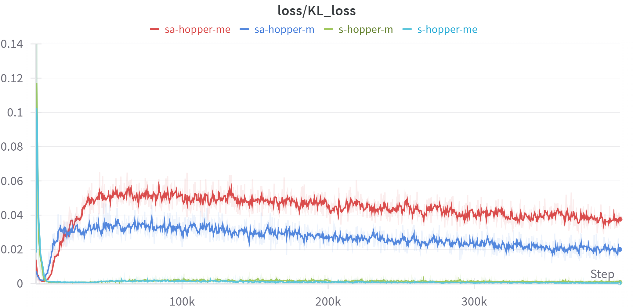
Figure 6: Illustration of the posterior collapse of C-VAE structure The blue curve represents the normal KL loss term while the green term represents the posterior collapse situation.

B.1.2. VAE implementations

For the C-VAE module, we employ the same VAE structure as Xu [Xu, Zhan, and Zhu, 2022] except that we change the input to (state, action) and the output to next state. Furthermore, we adopt the KL-annealing technique in the hopper environments where we do not introduce the KL loss initially by manually setting it to zero and slowly increasing the KL loss weight with time. KL-annealing could result in more abundant representations of the encoder and is less likely to introduce posterior collapse. We also simplify the decoder of the C-VAE module in hopper and walker2d environments to avoid posterior collapse. Notably, avoid to normalize the states and the actions because the normalized states are highly likely to result in the posterior collapse. In terms of experimental experience, the algorithm performs best when the KL loss converges to around 0.03. The information of next state is supplemented in the training phase to better model the offline distribution and statistical techniques are combined with neural networks to obtain more reasonable probability estimation.

B.1.3. Practical VAE distribution

In practice implementation, the offline data is the input to C-VAE model, and the statistical result of output from the C-VAE model, including mean and standard, are shown in the Figure 7.

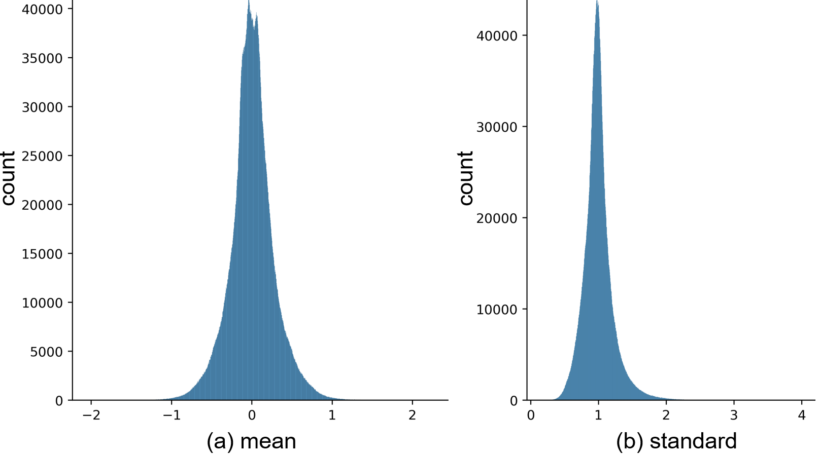
Figure 7: Statistical results of the output from the C-VAE model, including (a) the mean values and (b) the standard values

A.2. Embedding network

The embedding network structure is inspired by the work of Badia [Badia et al., 2019], where this network is introduced to extract valuable information from two successive states and predict the probability of all the actions. Thinking that we need to model the offline distribution of the state-action pairs, it is inspiring to construct a representation from two structurally consistent and logically connected states to predict the actions with different structures. It is worth noting that Badia only discusses the discrete environments, implying that the actions are represented with one-hot encoding. However, the pipeline conflicts with our setting that the state and action are continuous, we modify the embedding network by computing the loss with the real action values instead of the action representations. In practice, we train a Siamese network to get the controllable states and utilize the controllable states representation to predict the offline probability of each action, termed as the conditional likelihood $p_{o}(a|s_{k},s_{k+1})$, where $h$ is a classifier network followed by a ReLU layer (different from the softmax layer from Badia because the range of actions is not (0, 1)). Therefore, we could only get the loss term instead of the probability because we substituted the softmax layer for ReLU layer. So we also calculate the output of the offline dataset and model the data with a normal distribution, like that in the C-VAE.

Appendix C C. Algorithm Implementation

C.1. SAMG implementation on baselines

To illustrate the whole procedure of SAMG, we first represent the pseudo-code of SAMG implemented based on AWAC [Nair et al., 2020] below:

1:offline Q-network $Q_{\phi}^{off}$, policy $\pi_{\theta}^{off}$ and VAE

2:$\pi_{\theta}\leftarrow\pi_{\theta}^{off}$ , $Q_{\phi}\leftarrow Q_{\phi}^{off}$

3:Initialize the replay buffer $D$ with $N$ samples collected by $Q_{\phi}$

4:for iteration $i=1,2,...$ do

5:     for every environment step do

6:         $a_{t}\sim\pi_{\phi}(s_{t}|s_{t})$

7:         $s_{t+1},d_{t}\sim p_{(}s_{t+1}|s_{t},a_{t})$

8:         insert $(s_{t},a_{t},r(s_{t},a_{t}),s_{t+1},d_{t})$ into D

9:     end for

10:     for every update step do

11:         get $Q_{target}$ and $Q_{target}^{off}$ according to AWAC

12:         get $p_{om}$ with C-VAE according to Section Distribution-aware weight

13:         $Q_{target}\leftarrow(1-p_{om})Q_{target}+p_{om}Q_{target}^{off}$

14:         Update $\phi$ according to Eq. 9 in [Nair et al., 2020] with $Q_{target}$

15:         Update $\theta$ according to Eq. 13 in [Nair et al., 2020]

16:     end for

17:end for

Only some minimal adjustments are needed to implement SAMG on AWAC, and IQL [Kostrikov, Nair, and Levine, 2022] as well. We just need to maintain a much smaller replay buffer filled with online samples and insert and sample from this "online replay buffer". Before conducting normal gradient update step, we need to calculate the mixed $Q_{target}$ according to 4. As for IQL, we freeze and query the offline pre-trained value function instead because IQL separately trains a value function to serve as the target information. Other implementations are similar to AWAC and are omitted.

As for CQL and Cal_QL, these two algorithms share a similar implementation procedure and align with AWAC when calculating the $Q_{target}$. However, CQL adds one extra penalty term to minimize the expected Q-value based on a distribution $\mu(a|s)$, formulated as $\mathbb{E}_{s\sim\mathcal{D},a\sim\mu(a|s)}\left[Q(s,a)\right]$. This term is separated from the standard Bellman equation and serves an important role in making sure the learned Q-function is lower-bounded. However, this term is unrestricted in our paradigm and may cause algorithm divergence. So we add an offline version of the term still weighted by the distribution-aware weight. This slightly avoids our setting but is reasonable that this setting shares the consistent updating direction with the Bellman equation error term.

We implement all the algorithms based on the benchmark CORL [Tarasov et al., 2024], whose open source code is available at https://github.com/tinkoff-ai/CORL and the license is Apache License 2.0 with detail in the GitHub link.

C.2. Implementation Details

In practice, we strictly adopt the CORL setting to train the offline model and the vanilla fine-tuning training, including the training process and hyperparameters. In the fine-tuning process, training for all algorithms other than IQL is conducted for 500,000 steps, while IQL is conducted for 1,000,000 steps. As for SAMG training, for mujoco environments (halfcheetah, hopper, walker2d), SAMG algorithms share the same set of hyperparameters with the fine-tuning process to illustrate fairness. In the antmaze environment, we slightly reduce the weight of the Q-value maximization term to highlight the impact of SAMG for algorithms CQL and Cal_QL, from 5 to 2-3. For the threshold $p_{om}$, we have shown in Section Sensitivity analysis of threshold $p_{om}$ that it is not sensitive in most environments, we adopt the value of 0.5 in most environments which seems large but only a small portion satisfies the condition. For the antmaze environment, we take 0.4 for Cal_QL and 0.5 for CQL. We maintain an online replay buffer with a small capacity (only 50,000) and initialize it with 1000 samples utilizing the offline model (1000 is the normal length of an episode in most environments). The details of C-VAE are jointly stated in Appendix B.

C.3. Datasets

D4RL (Datasets for Deep Data-Driven Reinforcement Learning) [Fu et al., 2020] is a standard benchmark including a variety of environments. SAMG is tested across four environments within D4RL: HalfCheetah, hopper, walker2d and antmaze.

1. HalfCheetah: The halfcheetah environments simulates a two-legged robot similar to a cheetah, but only with the lower half of the cheetah. The goal is to navigate and move forward by coordinating the movements of its two legs. It is a challenging environment due to the complex dynamics of the motivation.

2. Hopper: In the Hopper environment, the agent is required to control a one-legged hopping robot, whose objective is similar to that of the HalfCheetah. The agent needs to learn to make the hopper move forward while maintaining balance and stability. The Hopper environment presents challenges related to balancing and controlling the hopping motion.

3. Walker2d: Walker2d is an environment controlling a two-legged robot, which resembles a simplified human walker. The goal of Walker2d is to move the walker forward while maintaining stability. walker2d poses challenges similar to HalfCheetah environment but introduces additional complexities related to humanoid structure. The above three environments have three different levels of datasets, including medium-expert, medium-replay, medium.

4. AntMaze: In the AntMaze environment, the agent controls an ant-like robot to navigate through maze-like environments to reach a goal location. The agent receives a sparse reward that the agent only receives a positive reward when it successfully reaches the goal. this makes the task more difficult. The maze configurations vary from the following environments that possess different level of complexity, featuring dead ends and obstacles. There are totally six different levels of datasets, including: maze2d-umaze, maze2d-umaze-diverse, maze2d-medium-play, maze2d-medium-diverse, maze2d-large-play, maze2d-large-diverse.

C.4. SAMG performance

As illustrated in Section Empirical results, SAMG performs best when integrated with AWAC compared to other algorithms.

The reason why AWAC-SAMG performs the best is detailed below. AWAC stands for advantage weighted actor critic, which is an algorithm to optimize the advantage function $A^{\pi_{k}}(s,a)$, while constraining the policy to stay close to offline data. AWAC does not contain any other tricks to under-estimate the value function as other offline RL algorithms [Kumar et al., 2020, Nakamoto et al., 2023], therefore AWAC could produce an accurate estimation of the values of offline data and serves as a perfect partner of SAMG.

For the other algorithms, they adopt various techniques to achieve conservative estimation of $Q$ values in order to counteract the potential negative effects of OOD samples. Therefore, the offline guidance they provide is a little less accurate. However, these algorithms are more robust due to conservative settings and can cope with more complex tasks, as illustrated in Section 5 of CQL [Kumar et al., 2020]. However, it is always impossible to produce ideal $Q$ values for offline RL algorithms due to the limitations of offline datasets. The offline models trained by these algorithms could still provide guidance for the online fine-tuning process because the error of the estimation is trivial and the guidance is valuable and reliable. Furthermore, to resist the negative impact of conservative estimation, we cut the offline guidance and revert to the vanilla algorithms after a specific period of time in practice.

Overall, SAMG is a novel and effective paradigm, which is coherently conformed by theoretical analysis and abundant experiments.

C.5. Cumulative regret

The cumulative regrets of the Antmaze environment of four vanilla algorithms and SAMG are shown in the Table 2.

It can be concluded from the table that SAMG possesses significantly lower regret than the vanilla algorithms, at least 40.12% of the vanilla algorithms in the scale. This illustrate the effectiveness of our algorithms in utilizing online samples and experimentally demonstrates the superiority of SAMG paradigm.

Table 2: Cumulative regret of online fine-tuning algorithms. The cumulative regret of standard base algorithms (including CQL, IQL, AWAC and Cal_QL, denoted as "Vanilla") compared to SAMG integrated algorithms (referred to as "Ours").

Dataset	CQL		AWAC		IQL		Cal-QL
	Vanilla	Ours	Vanilla	Ours	Vanilla	Ours	Vanilla	Ours
antmaze-u	0.051(0.005)	0.021(0.002)	0.081(0.046)	0.080(0.021)	0.072(0.005)	0.063(2.0)	0.023(0.003)	0.031(0.002)
antmaze-ud	0.185(0.061)	0.191(0.075)	0.875(0.046)	0.378(0.090)	0.392(0.116)	0.182(0.021)	0.142(0.124)	0.133(0.091)
antmaze-md	0.148(0.004)	0.131(0.010)	1.0(0.0)	1.0(0.0)	0.108(0.007)	0.102(0.008)	0.069(0.012)	0.076(0.025)
antmaze-mp	0.136(0.023)	0.078(0.369)	1.0(0.0)	1.0(0.0)	0.115(0.009)	0.143(0.020)	0.057(0.009)	0.071(0.008)
antmaze-ld	0.359(0.036)	0.382(0.023)	1.0(0.0)	1.0(0.0)	0.367(0.033)	0.305(0.041)	0.223(0.111)	0.219(0.157)
antmaze-lp	0.344(0.023)	0.317(0.052)	1.0(0.0)	1.0(0.0)	0.335(0.032)	0.321(0.043)	0.203(0.095)	0.211(0.114)

C.6. Unsatisfactory performance on particular environment

We think the hyperparameter $\tau$ and the environment property may account for the unsatisfactory performance of IQL-SAMG on the environment Halfcheetah-medium-expert, rather than the integration of IQL and SAMG.

In detail, as stated in the paper on IQL, the estimated function will gain on the optimal value as $\tau\to 1$. However, $\tau$ is not chosen to be 1 in practice and is quite low in the poorly performing environment. Additionally, this environment is relatively narrow and the training score is abnormally higher than the evaluation score. Therefore, we believe the unsatisfactory performance in this environment is just an exception and does not indicate problems of the SAMG paradigm.

C.7. Method to get the data coverage rate of offline dataset

To get the data coverage of a specific dataset, we aggregate all levels of datasets of a given environment, i.e., expert, medium-expert, medium-replay, medium, random level of datasets of environments HalfCheetah, Hopper, Walker2d. Thinking that the state and action are high-dimensional, we first perform dimensionality reduction. We uniformly and randomly select part of the data due to its huge scale and then perform t-SNE [Van der Maaten and Hinton, 2008] separately on the actions and states of this subset for dimensionality reduction. Given that it is hard to model the distribution of the continuous dimensional-reduced data, We then conduct hierarchical clustering [Müllner, 2011] to calculate and analyze the distribution of the data. We compute the clustering results of each environment and calculate the coverage rate based on the clustering results. To be specific, we select 10 percent of all data each time to cluster and repeat this process for 10 random seeds. For each clustering result, we calculate the data coverage rate of each level of offline dataset by counting the proportion of clustering center points. We consider one level of offline dataset to possess a clustering center if there exists more than 50 samples labeled with this clustering center.

Appendix D D. Compute resources

All the experiments in this paper are conducted on a linux server with Intel(R) Xeon(R) Gold 6226R CPU @ 2.90GHz and NVIDIA Geforce RTX 3090. We totally use 8 GPU in the experiments and each experiment takes one GPU and roughly occupies around 30% of the GPU. It takes approximately 3 hours to 24 hours to run an experiment on one random seed, depending on the specific algorithms and environments. Specifically, the average time cost of experiments on Mujoco environments (HalfCheetah, Hopper, Walker2d) is 4.5 hours while it takes an average time of 20 hours in environment AntMaze. All experiments took a total of two months. Approximately ten days were spent on exploration, while twenty days were dedicated to completing preliminary offline algorithms.

References

- Aytar et al. [2018] Aytar, Y.; Pfaff, T.; Budden, D.; Paine, T.; Wang, Z.; and de Freitas, N. 2018. Playing hard exploration games by watching YouTube. In Advances in Neural Information Processing Systems.
- Badia et al. [2019] Badia, A. P.; Sprechmann, P.; Vitvitskyi, A.; Guo, D.; Piot, B.; Kapturowski, S.; Tieleman, O.; Arjovsky, M.; Pritzel, A.; Bolt, A.; et al. 2019. Never Give Up: Learning Directed Exploration Strategies. In International Conference on Learning Representations.
- Baker et al. [2022] Baker, B.; Akkaya, I.; Zhokov, P.; Huizinga, J.; Tang, J.; Ecoffet, A.; Houghton, B.; Sampedro, R.; and Clune, J. 2022. Video pretraining (vpt): Learning to act by watching unlabeled online videos. Advances in Neural Information Processing Systems, 35: 24639–24654.
- Beeson and Montana [2022] Beeson, A.; and Montana, G. 2022. Improving TD3-BC: Relaxed Policy Constraint for Offline Learning and Stable Online Fine-Tuning. arXiv preprint arXiv:2211.11802.
- Bowman et al. [2015] Bowman, S. R.; Vilnis, L.; Vinyals, O.; Dai, A. M.; Jozefowicz, R.; and Bengio, S. 2015. Generating sentences from a continuous space. arXiv preprint arXiv:1511.06349.
- Chen et al. [2020] Chen, X.; Zhou, Z.; Wang, Z.; Wang, C.; Wu, Y.; and Ross, K. 2020. Bail: Best-action imitation learning for batch deep reinforcement learning. Advances in Neural Information Processing Systems, 33: 18353–18363.
- Dvoretzky [1959] Dvoretzky, A. 1959. A theorem on convex bodies and applications to Banach spaces. Proceedings of the National Academy of Sciences, 45(2): 223–226.
- Fu et al. [2020] Fu, J.; Kumar, A.; Nachum, O.; Tucker, G.; and Levine, S. 2020. D4RL: Datasets for deep data-driven reinforcement learning. arXiv preprint arXiv:2004.07219.
- Fujimoto and Gu [2021] Fujimoto, S.; and Gu, S. S. 2021. A minimalist approach to offline reinforcement learning. Advances in neural information processing systems, 34: 20132–20145.
- Fujimoto, Meger, and Precup [2019] Fujimoto, S.; Meger, D.; and Precup, D. 2019. Off-Policy Deep Reinforcement Learning without Exploration. In Proceedings of the 36th International Conference on Machine Learning.
- Haarnoja et al. [2018] Haarnoja, T.; Zhou, A.; Abbeel, P.; and Levine, S. 2018. Soft actor-critic: Off-policy maximum entropy deep reinforcement learning with a stochastic actor. In International conference on machine learning, 1861–1870. PMLR.
- Hester et al. [2018] Hester, T.; Vecerik, M.; Pietquin, O.; Lanctot, M.; Schaul, T.; Piot, B.; Horgan, D.; Quan, J.; Sendonaris, A.; Osband, I.; et al. 2018. Deep q-learning from demonstrations. In Thirty-Second AAAI Conference on Artificial Intelligence.
- Iman, Arabnia, and Rasheed [2023] Iman, M.; Arabnia, H. R.; and Rasheed, K. 2023. A review of deep transfer learning and recent advancements. Technologies, 11(2): 40.
- Janner et al. [2019] Janner, M.; Fu, J.; Zhang, M.; and Levine, S. 2019. When to trust your model: Model-based policy optimization. In Advances in Neural Information Processing Systems, 12498–12509.
- Kang, Jie, and Feng [2018] Kang, B.; Jie, Z.; and Feng, J. 2018. Policy optimization with demonstrations. In International conference on machine learning, 2469–2478. PMLR.
- Keeler and Meir [1969] Keeler, E.; and Meir, A. 1969. A theorem on contraction mappings. J. Math. Anal. Appl, 28: 326–329.
- Kingma et al. [2014] Kingma, D. P.; Mohamed, S.; Jimenez Rezende, D.; and Welling, M. 2014. Semi-supervised learning with deep generative models. Advances in neural information processing systems, 27.
- Kostrikov, Nair, and Levine [2022] Kostrikov, I.; Nair, A.; and Levine, S. 2022. Offline Reinforcement Learning with Implicit Q-Learning. In International Conference on Learning Representations.
- Kumar et al. [2019] Kumar, A.; Fu, J.; Soh, M.; Tucker, G.; and Levine, S. 2019. Stabilizing off-policy q-learning via bootstrapping error reduction. In Advances in Neural Information Processing Systems, 11761–11771.
- Kumar et al. [2020] Kumar, A.; Zhou, A.; Tucker, G.; and Levine, S. 2020. Conservative q-learning for offline reinforcement learning. Advances in Neural Information Processing Systems, 33: 1179–1191.
- Lee et al. [2022] Lee, S.; Seo, Y.; Lee, K.; Abbeel, P.; and Shin, J. 2022. Offline-to-online reinforcement learning via balanced replay and pessimistic q-ensemble. In Conference on Robot Learning, 1702–1712. PMLR.
- Levine et al. [2020] Levine, S.; Kumar, A.; Tucker, G.; and Fu, J. 2020. Offline reinforcement learning: Tutorial, review, and perspectives on open problems. arXiv preprint arXiv:2005.01643.
- Li et al. [2023] Li, J.; Liu, X.; Zhu, B.; Jiao, J.; Tomizuka, M.; Tang, C.; and Zhan, W. 2023. Guided Online Distillation: Promoting Safe Reinforcement Learning by Offline Demonstration.
- Lifshitz et al. [2024] Lifshitz, S.; Paster, K.; Chan, H.; Ba, J.; and McIlraith, S. 2024. Steve-1: A generative model for text-to-behavior in minecraft. Advances in Neural Information Processing Systems, 36.
- Lowrey et al. [2019] Lowrey, K.; Rajeswaran, A.; Kakade, S.; Todorov, E.; and Mordatch, I. 2019. Plan Online, Learn Offline: Efficient Learning and Exploration via Model-Based Control. In International Conference on Learning Representations.
- Lucas et al. [2019] Lucas, J.; Tucker, G.; Grosse, R.; and Norouzi, M. 2019. Understanding Posterior Collapse in Generative Latent Variable Models.
- Lyu et al. [2022] Lyu, J.; Ma, X.; Li, X.; and Lu, Z. 2022. Mildly Conservative Q-Learning for Offline Reinforcement Learning. In Oh, A. H.; Agarwal, A.; Belgrave, D.; and Cho, K., eds., Advances in Neural Information Processing Systems.
- Mao et al. [2022] Mao, Y.; Wang, C.; Wang, B.; and Zhang, C. 2022. Moore: Model-based offline-to-online reinforcement learning. arXiv preprint arXiv:2201.10070.
- Mark et al. [2022] Mark, M. S.; Ghadirzadeh, A.; Chen, X.; and Finn, C. 2022. Fine-tuning Offline Policies with Optimistic Action Selection. In Deep Reinforcement Learning Workshop NeurIPS 2022.
- Müllner [2011] Müllner, D. 2011. Modern hierarchical, agglomerative clustering algorithms. arXiv preprint arXiv:1109.2378.
- Nair et al. [2020] Nair, A.; Dalal, M.; Gupta, A.; and Levine, S. 2020. Accelerating Online Reinforcement Learning with Offline Datasets. arXiv preprint arXiv:2006.09359.
- Nair et al. [2018] Nair, A.; McGrew, B.; Andrychowicz, M.; Zaremba, W.; and Abbeel, P. 2018. Overcoming Exploration in Reinforcement Learning with Demonstrations. In IEEE International Conference on Robotics and Automation.
- Nakamoto et al. [2023] Nakamoto, M.; Zhai, Y.; Singh, A.; Ma, Y.; Finn, C.; Kumar, A.; and Levine, S. 2023. Cal-QL: Calibrated Offline RL Pre-Training for Efficient Online Fine-Tuning. In Workshop on Reincarnating Reinforcement Learning at ICLR 2023.
- Prudencio, Maximo, and Colombini [2023] Prudencio, R. F.; Maximo, M. R.; and Colombini, E. L. 2023. A survey on offline reinforcement learning: Taxonomy, review, and open problems. IEEE Transactions on Neural Networks and Learning Systems.
- Rafailov et al. [2023] Rafailov, R.; Hatch, K. B.; Kolev, V.; Martin, J. D.; Phielipp, M.; and Finn, C. 2023. MOTO: Offline to Online Fine-tuning for Model-Based Reinforcement Learning. In Workshop on Reincarnating Reinforcement Learning at ICLR 2023.
- Rajeswaran et al. [2018] Rajeswaran, A.; Kumar, V.; Gupta, A.; Vezzani, G.; Schulman, J.; Todorov, E.; and Levine, S. 2018. Learning complex dexterous manipulation with deep reinforcement learning and demonstrations. In Robotics: Science and Systems.
- Schaal [1996] Schaal, S. 1996. Learning from demonstration. Advances in neural information processing systems, 9.
- Song et al. [2023] Song, Y.; Zhou, Y.; Sekhari, A.; Bagnell, D.; Krishnamurthy, A.; and Sun, W. 2023. Hybrid RL: Using both offline and online data can make RL efficient. In The Eleventh International Conference on Learning Representations.
- Sutton [1988] Sutton, R. S. 1988. Learning to predict by the methods of temporal differences. Machine learning, 3: 9–44.
- T. Jaakkola and Singh [1994] T. Jaakkola, M. I. J.; and Singh, S. P. 1994. On the Convergence of Stochastic Iterative Dynamic Programming Algorithms. Neural Computation, 6.
- Tarasov et al. [2024] Tarasov, D.; Nikulin, A.; Akimov, D.; Kurenkov, V.; and Kolesnikov, S. 2024. CORL: Research-oriented deep offline reinforcement learning library. Advances in Neural Information Processing Systems, 36.
- Thomas [2014] Thomas, P. 2014. Bias in natural actor-critic algorithms. In International conference on machine learning, 441–448. PMLR.
- Van der Maaten and Hinton [2008] Van der Maaten, L.; and Hinton, G. 2008. Visualizing data using t-SNE. Journal of machine learning research, 9(11).
- Vecerik et al. [2017] Vecerik, M.; Hester, T.; Scholz, J.; Wang, F.; Pietquin, O.; Piot, B.; Heess, N.; Rothörl, T.; Lampe, T.; and Riedmiller, M. 2017. Leveraging demonstrations for deep reinforcement learning on robotics problems with sparse rewards. arXiv preprint arXiv:1707.08817.
- Wang et al. [2024] Wang, S.; Yang, Q.; Gao, J.; Lin, M.; Chen, H.; Wu, L.; Jia, N.; Song, S.; and Huang, G. 2024. Train once, get a family: State-adaptive balances for offline-to-online reinforcement learning. Advances in Neural Information Processing Systems, 36.
- Wang, Blei, and Cunningham [2021] Wang, Y.; Blei, D.; and Cunningham, J. P. 2021. Posterior collapse and latent variable non-identifiability. Advances in Neural Information Processing Systems, 34: 5443–5455.
- Weiss, Khoshgoftaar, and Wang [2016] Weiss, K.; Khoshgoftaar, T. M.; and Wang, D. 2016. A survey of transfer learning. Journal of Big data, 3: 1–40.
- Wu et al. [2022] Wu, J.; Wu, H.; Qiu, Z.; Wang, J.; and Long, M. 2022. Supported Policy Optimization for Offline Reinforcement Learning. arXiv preprint arXiv:2202.06239.
- Xu, Zhan, and Zhu [2022] Xu, H.; Zhan, X.; and Zhu, X. 2022. Constraints penalized q-learning for safe offline reinforcement learning. In Proceedings of the AAAI Conference on Artificial Intelligence.
- Yu et al. [2021] Yu, T.; Kumar, A.; Rafailov, R.; Rajeswaran, A.; Levine, S.; and Finn, C. 2021. Combo: Conservative offline model-based policy optimization. Advances in neural information processing systems, 34: 28954–28967.
- Yuan et al. [2024] Yuan, H.; Mu, Z.; Xie, F.; and Lu, Z. 2024. Pre-Training Goal-based Models for Sample-Efficient Reinforcement Learning. In The Twelfth International Conference on Learning Representations.
- Zhu et al. [2019] Zhu, H.; Gupta, A.; Rajeswaran, A.; Levine, S.; and Kumar, V. 2019. Dexterous manipulation with deep reinforcement learning: Efficient, general, and low-cost. In 2019 International Conference on Robotics and Automation (ICRA), 3651–3657. IEEE.
- Zhu et al. [2018] Zhu, Y.; Wang, Z.; Merel, J.; Rusu, A.; Erez, T.; Cabi, S.; Tunyasuvunakool, S.; Kramár, J.; Hadsell, R.; de Freitas, N.; et al. 2018. Reinforcement and imitation learning for diverse visuomotor skills. arXiv preprint arXiv:1802.09564.