Supercritical McKean-Vlasov SDE driven by cylindrical $\alpha$-stable process

Abstract.

In this paper, we study the following supercritical McKean-Vlasov SDE, driven by a symmetric non-degenerate cylindrical $\alpha$-stable process in $\mathbb{R}^{d}$ with $\alpha\in(0,1)$:

$$\mathord{{\rm d}}X_{t}=(K*\mu_{t})(X_{t})\mathord{{\rm d}}t+\mathord{{\rm d}}L_{t}^{(\alpha)},\quad X_{0}=x\in\mathbb{R}^{d},$$

where $K:\mathbb{R}^{d}\to\mathbb{R}^{d}$ is a $\beta$-order Hölder continuous function, and $\mu_{t}$ represents the time marginal distribution of the solution $X$. We establish both strong and weak well-posedness under the conditions $\beta\in(1-\alpha/2,1)$ and $\beta\in(1-\alpha,1)$, respectively. Additionally, we demonstrate strong propagation of chaos for the associated interacting particle system, as well as the convergence of the corresponding Euler approximations. In particular, we prove a commutation property between the particle approximation and the Euler approximation.

1. Introduction

In recent years, distribution-dependent stochastic differential equations (abbreviated as DDSDEs) have attracted more and more interest, and one important reason is that DDSDEs are deeply related to nonlinear Fokker-Planck equations, which also remain an important area in analysis since they come from many physical and biological models. In the literature, DDSDEs are also often referred to as McKean-Vlasov stochastic differential equations (cf. [Kac56, Kac59, Mc66]). We refer to the article [HRW21] for more about the history and updates on the study of DDSDEs.

In this paper, we devote to establishing well-posedness as well as numerical approximations (propagation of chaos and Euler’s approximations) for a class of DDSDEs which have Hölder interaction kernels and are driven by symmetric non-degenerate $\alpha$-stable processes with $\alpha\in(0,1)$. Precisely, we consider the following McKean-Vlasov SDEs in ${\mathbb{R}}^{d}$ with $d\geqslant 1$:

$${\mathord{{\rm d}}}X_{t}=(K*\mu_{t})(X_{t}){\mathord{{\rm d}}}t+{\mathord{{\rm d}}}L_{t}^{(\alpha)},$$ (1.1)

where $K:{\mathbb{R}}^{d}\to{\mathbb{R}}^{d}$ is some Hölder continuous function, and $\mu_{t}$ is the time marginal distribution of the process $(X_{t})_{t\geqslant 0}$, and the asterisk denotes the spatial convolution,

$$(K*\mu_{t})(x):=\int_{{\mathbb{R}}^{d}}K(x-y)\mu_{t}({\mathord{{\rm d}}}y),$$

and $(L_{t}^{(\alpha)})_{t\geqslant 0}$ is an $\alpha$-stable process on some probability space $(\Omega,{\mathscr{F}},{\mathbb{P}})$, having a Lévy measure $\nu^{(\alpha)}$ with the following form:

$$\nu^{(\alpha)}(A)=\int^{\infty}_{0}\left(\int_{{\mathbb{S}}^{d-1}}\frac{1_{A}(r\theta)\Sigma({\mathord{{\rm d}}}\theta)}{r^{1+\alpha}}\right){\mathord{{\rm d}}}r,\quad A\in{\mathscr{B}}({\mathbb{R}}^{d}),$$ (1.2)

where $\Sigma$ is a finite measure over the unit sphere ${\mathbb{S}}^{d-1}$ (called spherical measure of $\nu^{(\alpha)}$), and ${\mathscr{B}}({\mathbb{R}}^{d})$ is the Borel $\sigma$-algebra on ${\mathbb{R}}^{d}$.

1.1. Motivation

Supposing $\mu_{t}({\mathord{{\rm d}}}x)=\varrho_{t}(x){\mathord{{\rm d}}}x$ in SDE (1.1), by Itô’s formula, formally, one sees that $\varrho_{t}$ solves the following nonlocal nonlinear Fokker-Planck equation in the distributional sense:

$$\partial_{t}\varrho_{t}=({\mathscr{L}}^{(\alpha)})^{*}\varrho_{t}-\mathord{{\rm div}\,}((K*\varrho_{t})\varrho_{t}),$$ (1.3)

where $({\mathscr{L}}^{(\alpha)})^{*}$ is the conjugate operator of the nonlocal operator ${\mathscr{L}}^{(\alpha)}$ defined by

$${\mathscr{L}}^{(\alpha)}f(x):=\int_{{\mathbb{R}}^{d}}{\Big{(}}f(x+z) -f(x){\Big{)}}\nu^{(\alpha)}({\mathord{{\rm d}}}z)$$ (1.4)

with $\alpha\in(0,1)$ and $f\in C_{b}^{1}({\mathbb{R}}^{d})$. Notice that when $\nu^{(\alpha)}({\mathord{{\rm d}}}z)=c/|z|^{d+\alpha}{\mathord{{\rm d}}}z$ with an appropriate constant, the operator ${\mathscr{L}}^{(\alpha)}$ is exactly the usual fractional Laplacian operator $\Delta^{\alpha/2}:=-(-\Delta)^{\alpha/2}$ on ${\mathbb{R}}^{d}$.

As mentioned at the beginning of this paper, the nonlinear partial differential equation (abbreviated as PDE) (1.3) has attracted extensive and increasing attention due to its relevance to various models from natural science. In a local Laplacian context, for instance, when $K(x)=\nabla\mathrm{e}^{-|x|}$ and $({\mathscr{L}}^{(\alpha)})^{*}\varrho_{t}$ is substituted with $\mathord{{\rm div}\,}(\varrho_{t}^{2}\nabla\varrho_{t})$, a so-called aggregation-diffusion equation was established in [TBL06] to model the dynamics of a population where individuals experience long range social attraction and short range dispersal. Considering the case ${\mathscr{L}}^{(\alpha)}=\Delta$ (the Laplace operator), when $d=2$ and $K(x)$ is taken as the Biot-Savart law $(-x_{2},x_{1})/|x|^{2}$, the equation (1.3) transforms into the famous vorticity form of the 2D Navier-Stokes equation. Moreover, in the same case ${\mathscr{L}}^{(\alpha)}=\Delta$, taking $K(x)\asymp|x|^{1-d}$, the equation is seen as the Keller-Segel chemotaxis model (see [AT21] for example). Back to nonlocal cases, in the fractional Laplace framework, PDE (1.3) reads the surface quasi-geostrophic equation in the mathematical theory of meteorology and oceanography if $K(x)=(-x_{2},x_{1})/|x|^{3}$ on ${\mathbb{R}}^{2}$ and ${\mathscr{L}}^{(\alpha)}=\Delta^{\alpha/2}$. For further insights into these models and their applications, we refer readers to [BLR11, HRZ23] and the references therein. Moreover, in the context of the inviscid case, where the diffusive term $({\mathscr{L}}^{(\alpha)})^{*}\varrho_{t}$ is omitted, and the interaction kernel $K$ exhibits Hölder continuous at the origin, specifically $K(x)\sim|x|^{\beta}$ with some $\beta\geqslant 0$, the well-posedness of the aggregation equation (1.3) was also studied in the literature, such as [CDFLS] the references therein. See also [BLR11] for the $L^{p}$ kernels. It should be noted that the initial data $\mu_{0}$ is always assumed regular in these studies.

On the other hand, the McKean-Vlasov SDE (1.1) can be derived from the following large particle systems:

$${\mathord{{\rm d}}}X^{N,j}_{t}=\frac{1}{N}\sum_{i=1}^{N}K(X^{N,j}_{t}-X^{N,i}_{t}){\mathord{{\rm d}}}t+{\mathord{{\rm d}}}L^{(\alpha),j}_{t},$$ (1.5)

where $N\in{\mathbb{N}}$, and $j=1,2,\cdots,N$, and the interaction kernel $K$ within the systems models attraction and repulsion interactions between each two particles, and $\{L^{(\alpha),j}\}_{j=1}^{\infty}$ is a family of i.i.d. $\alpha$-stable processes with the same law as $L^{(\alpha)}$, which represents random phenomena. As a matter of fact, back to the 1950s, using $N$-particle systems, Kac (cf. [Kac56]) derived the spactially homogeneous Boltzmann equation, and to this end, the classical notion of propagation of (Kac’s) chaos was formalized. We also refer to the Lecture notes [Szn91] and review paper [CD22] for more details of propagation of chaos. It should be noted that in the study of Boltzmann equation, the pure jump process, like $\alpha$-stable processes, play an important role (see [Ta78] for example). Additionally, notice that the scaling factor $\frac{1}{N}$, which is critical in ensuring convergences of these systems as $N\to\infty$, is referred to as the mean-field scaling (for more details, see [Ja14, Section 1.1]). Consequently, DDSDEs are also termed as mean-field limit SDEs in the literature.

1.2. Problem statement: supercriticality

In this subsection, we discuss the supercriticality of SDEs when $\alpha\in(0,1)$.

1.2.1. What is supercriticality?

First of all, let us explain the meaning of supercriticality from the point of view of PDE. Let $\alpha\in(0,2)$. Replacing $(K*\mu_{t})(x)$ by a distribution-free drift $b(x)$ in SDE (1.1), we consider the following classical SDE:

$${\mathord{{\rm d}}}X_{t}=b(X_{t}){\mathord{{\rm d}}}t+{\mathord{{\rm d}}}L_{t}^{(\alpha)},$$ (1.6)

where the drift term $b$ belongs to the usual Hölder space ${\mathbf{C}}^{\beta}({\mathbb{R}}^{d})$ (see subsection 2.1 for the definitions) with $\beta\in(0,1)$. For simplicity, we assume that $\nu^{(\alpha)}({\mathord{{\rm d}}}z)=c/|z|^{d+\alpha}{\mathord{{\rm d}}}z$ in (1.2), where $c$ is an appropriate constant such that the infinitesimal generator of $X$ is given by

$$\Delta^{\alpha/2}+b\cdot\nabla.$$

On the one hand, it is well-known that the solution $u$ to the evolution equation

$$\partial_{t}u=\Delta^{\alpha/2}u,~{}~{}t>0,\quad\quad u(0)=\phi,$$

can be represented as $u(t,x)=p_{t}*\phi(x)$, where $p_{t}(x)$ is the smooth probability density function of the standard $\alpha$-stable process $L^{(\alpha)}$ (see, for example, [WH23]). This implies that, regardless of the singularity in the initial data $\phi$, the solution $u(t)$ becomes smooth for $t>0$. In contrast, for the transport equation

$$\partial_{t}u=b\cdot\nabla u,~{}~{}t>0,\quad\quad u(0)=\phi,$$ (1.7)

firstly, there is a well-known counterexample in the dimensional-one case,

$$b(x)=-2{\rm sign}(x)\sqrt{|x|},$$

where the drift term $b$ is only Hölder continuous but the Cauchy problem (1.7) has infinitely many solutions from any initial condition (cf. [FGP10, FGP18]). Interested readers are also refered to [MS24] for more literature and recent developments about the non-uniqueness of (stochastic) transport equations. Secondly, considering the simple case, the constant drift term $b\in{\mathbb{R}}^{d}$, one sees that the solution takes the form

$$u(t,x)=\phi(x+bt),$$

which indicates that the singularity of the initial data propagates into the solution when $t>0$. On the other hand, for the fractional Laplace $\Delta^{\alpha/2}$, the following scaling property holds:

$$\Delta^{\alpha/2}f(\lambda x)=\lambda^{\alpha}\Delta^{\alpha/2}f(x),\quad\forall\lambda>0.$$

Consequently, when $\alpha>1$, $\Delta^{\alpha/2}$ dominates, and the equation is said to be in the subcritical regime; when $\alpha\in(0,1)$, the gradient $b\cdot\nabla$ is of higher order than the fractional Laplacian, leading to the classification of the SDE as supercritical. The critical case corresponds to $\alpha=1$.

1.2.2. Challenges and methods

Notably, there is a well-known counterexample presented in [TTW74], which highlights that it is much more difficult to deal with the supercritical case than with the subcritical case. Rigorously speaking, in the one-dimensional case, Tanaka, Tsuchiya, and Watanabe [TTW74] established the strong well-posedness (strong existence and pathwise uniqueness) to the SDE (1.6) for any bounded measurable drift term $b$ in the subcritical regime $\alpha\in(1,2)$, and for any bounded continuous $b$ in the critical case $\alpha=1$. Furthermore, they demonstrated that in the supercritical case $\alpha\in(0,1)$, the strong well-posedness is ensured when $b$ is a bounded non-decreasing ${\mathbf{C}}^{\beta}$ function with $\beta>1-\alpha$. However, if $\beta+\alpha<1$, there exists a ${\mathbf{C}}^{\beta}$ function $b$ for which both pathwise uniqueness and uniqueness in law fail.

Samely, for the multi-dimensional case, following the strong well-posedness results obtained by [Pr12] under the subcritical regime conditioned on $\beta>1-\alpha/2$, solving the strong well-posedness problem in the supercritical regime has also proved to be a challenging task. Fortunately, this problem was progressively resolved in [CSZ18] for $\alpha\in(2/3,1)$, and later in [CMP20, HWW23] for $\alpha\in(1/2,1)$. Ultimately, the complete resolution of this problem was achieved by Chen, Zhang, and Zhao in [CZZ21], in which interested readers can find further details about the well-posedness of SDE (1.6).

Moreover, among the results mentioned above, a common approach is applying a priori estimates, such as Schauder’s estimates, of the corresponding PDE:

$$\partial_{t}u={\mathscr{L}}^{(\alpha)}u+b\cdot\nabla u+f.$$

In particular, to handle PDEs in the supercritical regime, the authors of [CZZ21] employed the energy method and Littlewood-Paley theory, where they established a Besov-type a priori estimate. This was subsequently extended to Schauder’s estimates in [SX23, Zh21].

In this paper, we consider supercritical $\alpha$-stable DDSDEs with drifts being $\beta$-Hölder continuous and depending on distributions. Especially, the weak and strong well-posedness hold for $\beta>1-\alpha$ and $\beta>1-\alpha/2$ respectively. The key ingredient in this paper is to establish a priori estimates about time regularity of the solution of the PDE (see Theorem 3.1 below), which was not studied in the previous works [CZZ21, SX23, Zh21].

1.3. Related works and our contributions

1.3.1. Well-posedness of DDSDEs

The first aim of this paper is to establish the well-posedness of the supercritical DDSDE (1.1) (see Theorem 1.3). It is well-known that the standard Brownian motion is also seen as a $2$-stable process, and has the infinitesimal generator ${\mathscr{L}}^{(\alpha)}$ being the classical Laplace operator $\Delta$ (cf. [Sa99]). Thus, in the following, we first briefly introduce some literature under the Brownian framework, and then discuss the jumped case.

To date, in the special case $\alpha=2$, both well-posedness (see [CF22, MV21, RZ21] for example) and propagation of chaos (e.g. [JW18, La21, HRZ24]) have been extensively investigated. To the best of our knowledge, there are at least four methods to study the well-posedness of DDSDEs, namely, the fixed point argument (see e.g. [Szn91]), the distribution iterations technique (cf. [Wa18]), the approach of Zvonkin’s transform and Krylov’s estimates (see [RZ21] for example), the bi-coupling method (see e.g. [HRW23]). Since we do not consider the Brownian case in this paper, we only list some literature here, and more details can be found in these works and the references therein.

Compared with the Brownian case, the McKean-Vlasov SDE (1.1) with noise being $\alpha$-stable and with the kernel $K$ being non-Lipschitz has received less attention. In the subcritical case $\alpha\in(1,2)$, the well-posedness theory of DDSDEs was considered in [BW99, DH23] and in [HRZ23] for second order models. As for the supercritical case $\alpha\in(0,1)$, to the best of our knowledge, there are only two works [FKKM21, DH24] studied well-posedness under the distributional-dependent framework. Regarding the McKean-Vlasov SDEs with Hölder interaction kernels, the authors, Frikha, Konakov, and Menozzi [FKKM21], established the well-posedness for $\alpha\in(2/3,2)$, which was, recently, extended to the case $\alpha\in(1/2,1]$ by Deng and Huang [DH24] via a fixed point method. It is worthy pointing out that these two works do not cover the whole supercritical regime $\alpha\in(0,1)$, and only considered the Lévy measure given by $\nu^{(\alpha)}({\mathord{{\rm d}}}z)\asymp{\mathord{{\rm d}}}z/|z|^{d+\alpha}$, where the Lévy noise is referred to as a standard $\alpha$-stable process.

It is important to note that the standard $\alpha$-stable process differs essentially from the Brownian motion, as the components of the former are not independent. When the components in an $\alpha$-stable process $(L^{(\alpha),1},..,L^{(\alpha),d})$ are independent $1$-dimensional $\alpha$-stable processes, the process will be called the cylindrical $\alpha$-stable process. We point out that cylindrical $\alpha$-stable processes play an important role not only in the $N$-particle system (1.5) but also in the related coupled i.i.d. system as given by

$${\mathord{{\rm d}}}X^{j}_{t}=(K*\mu^{j}_{t})(X^{j}_{t}){\mathord{{\rm d}}}t+{\mathord{{\rm d}}}L^{(\alpha),j}_{t},$$ (1.8)

which is important in the rest of this paper (see subsubsection 5.1.2), where the sequence $L^{(\alpha),1},...,L^{(\alpha),N},...$ consists of independent $\alpha$-stable processes. Hence, it is necessary to consider the cylindrical noise for DDSDE (1.1). On the other hand, obviously, the Lévy measure of the cylindrical $\alpha$-stable process has the following form:

$$\nu^{(\alpha)}({\mathord{{\rm d}}}z)\asymp\sum_{i=1}^{d}{\mathord{{\rm d}}}z_{i}/|z_{i}|^{1+\alpha}\delta_{0}({\mathord{{\rm d}}}\bar{z})$$

with the Dirac measure at zero $\delta_{0}$ on ${\mathbb{R}}^{d-1}$ and $\bar{z}:=(z_{1},..,z_{i-1},z_{i+1},...,z_{d})$, and is much more singular than the one of the standard $\alpha$-stable process. Moreover, from the point of view of Fourier analysis, the Fourier symbol of the associated operator ${\mathscr{L}}^{(\alpha)}=\sum_{j=1}^{d}\Delta_{j}^{\alpha/2}$ is given by $\sum_{j=1}^{d}|\xi_{j}|^{\alpha}$, which is notably more singular than $|\xi|^{\alpha}$, the symbol of the usual fractional Laplacian $\Delta^{\alpha/2}$, since the former one is not differentiable at each axis.

Contribution: In contrast to [FKKM21, DH24], we establish the well-posedness of DDSDE (1.1) with a large class of $\alpha$-stable processes including the standard ones and cylindrical ones (see the condition (ND) in the subsection 1.4), under the whole supercritical regime $\alpha\in(0,1)$ (see Theorem 1.3 below).

1.3.2. Numerical approximations of DDSDEs

Following the discussion on well-posedness, it is natural to consider suitable numerical approximations.

Recently, Euler-Maruyama approximations for singular SDEs have attracted significant attention (see [HW23] and the references therein for example). In particular, for DDSDEs, there have been several works, such as [WH23] for the subcritical Nemytskii-type case and [HRZ21, Zh19] for the Brownian case, that investigated the following Euler’s scheme for McKean-Vlasov SDEs: for $h\in(0,1)$, for $t\in[0,h]$, $X_{t}^{h}:=X_{0},$ and for $t\in[kh,(k+1)h]$ with $k=0,1,2,\cdots$,

$$X_{t}^{h}=X_{kh}^{h}+(K*\mu^{h}_{kh})(X^{h}_{kh})(t-kh)+L^{(\alpha)}_{t}-L^{(\alpha)}_{kh}.$$

Equivalently, the Euler approximation also can be seen as follows:

$$X^{h}_{t}=X_{0}+\int_{0}^{t}(K*\mu^{h}_{\pi_{h}(s)})(X^{h}_{\pi_{h}(s)}){\mathord{{\rm d}}}s+L^{(\alpha)}_{t},$$ (1.9)

where $\pi_{h}(t):=[t/h]h$, and $\mu^{h}_{\pi_{h}(t)}$ is the distribution of $X^{h}_{\pi_{h}(t)}$. Trivially, we have

$$X_{t}^{h}=X_{\pi_{h}(t)}^{h}+(K*\mu^{h}_{\pi_{h}(t)})(X^{h}_{\pi_{h}(t)})(t-\pi_{h}(t))+L^{(\alpha)}_{t}-L^{(\alpha)}_{\pi_{h}(t)}.$$

However, it is worth noting that simulating the distribution $\mu^{h}_{t}$ is more computationally challenging. Consequently, considering simulating the empirical measure, we see an Euler’s scheme for the $N$-particle systems (1.5), expressed as

$${\mathord{{\rm d}}}X^{N,j,h}_{t}=\frac{1}{N}\sum_{i=1}^{N}K(X^{N,j,h}_{\pi_{h}(t)}-X^{N,i,h}_{\pi_{h}(t)}){\mathord{{\rm d}}}t+{\mathord{{\rm d}}}L^{(\alpha),j}_{t},\ \ j=1,\dots,N.$$ (1.10)

Fixing the particle number $N$, we see that the process $(X^{N,1,h},\cdots,X^{N,N,h})$ is exactly an Euler approximation of a distributional-free SDE (see (1.14) for more detials). Now the situation becomes the distribution-free cylindrical case, in which there has been a lot of literature establishing the weak and strong Euler’s convergence $X^{N,j,h}\to X^{N,j}$ (as $h\to 0$), even for the supercritical case (cf. [BDG22, LZ23]).

Our second aim in this paper is to figure out the following commutative diagram, Figure 1, for all $\alpha\in(0,1)$ and $K\in{\mathbf{C}}^{\beta}({\mathbb{R}}^{d})$ with $\beta>1-\alpha$.

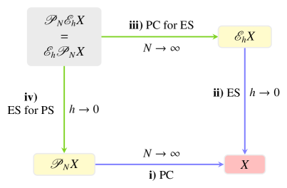
Figure 1. Propagation of chaos and Euler’s approximations

In this context, PC, PS, and ES stand for propagation of chaos, particle system, and Euler’s scheme respectively, and we set

$${\mathscr{E}}_{h}X:=X^{h},\quad\text{and}\quad{\mathscr{P}}_{N}X:=(X^{N,1},...,X^{N,N}),$$

and

$${\mathscr{P}}_{N}{\mathscr{E}}_{h}X={\mathscr{E}}_{h}{\mathscr{P}}_{N}X:=(X^{N,1,h},\ldots,X^{N,N,h}).$$

First of all, when the driven noise is a Brownian motion, all of ii), iii) and iv) in Figure 1 were studied in [Zh19] for bounded kernel via discrete Krylov’s estimates. In addition, the rest part, PC i) for singular kernels, also has been investigated well in recent years in both weak and strong sense. Interested readers can find the corresponding results in [JW18, La21, HRZ24]. As for the jumped case, there are fewer works. When the kernel $K$ is Lipschitz and $\alpha\in(1,2)$, the PC i) has been obtained in [Gr92], and the commutative diagram was established in [HY21, FL21]. Moreover, the author in [Ca22] obtained the PC i) with $\alpha>1$ and Hölder continuous kernel. The Euler approximation iv) in the strong (path) sense with rate was given by [LZ23] for additive noises under the conditions $K\in{\mathbf{C}}^{\beta}$ with $\beta>1-\alpha/2$ and $\alpha\in(0,2)$ (see [MX18] for multiplicative case under $\alpha\geqslant 1$).

Contribution: In this paper, we complete commutative diagram Figure 1 for the supercritical DDSDEs driven by non-degenerate symmetric $\alpha$-stable processes (e.g. the cylindrical ones, see the condition (ND) in subsection 1.4), where the interaction kernel $K$ exhibits $\beta$-Hölder continuous with $\beta>1-\alpha$. All the convergences are proved both in the weak sense (see Theorem 1.4 and Theorem 1.5 below), and the strong sense (see Theorem 1.6 below). Here, we would like to highlight the significance of the condition $K(x)\sim|x|^{\beta}\in{\mathbf{C}}^{\beta}({\mathbb{R}}^{d})$, as it proves valuable in several aggregation models discussed in subsection 1.1.

1.4. Main results

Before presenting our main results about supercritical DDSDEs, we introduce some notations and basic assumptions. In the sequel, we denote by ${\mathcal{P}}({\mathbb{R}}^{d})$ the space consisting of all probability measures on ${\mathbb{R}}^{d}$. Let $L^{(\alpha)}$ be an $\alpha$-stable process whose Lévy measure $\nu^{(\alpha)}({\mathord{{\rm d}}}z)$ given by (1.2) is symmetric in the sense of $\nu^{(\alpha)}(A)=\nu^{(\alpha)}(-A)$, $\forall A\in{\mathscr{B}}({\mathbb{R}}^{d})$. Note that for any $\gamma_{2}>\alpha>\gamma_{1}\geqslant 0$,

$$\int_{|z|\leqslant 1}|z|^{\gamma_{2}}\nu^{(\alpha)}({\mathord{{\rm d}}}z)+\int_{|z|>1}|z|^{\gamma_{1}}\nu^{(\alpha)}({\mathord{{\rm d}}}z)<\infty,$$

that is

$$\int_{{\mathbb{R}}^{d}}[|z|^{\gamma_{1}}\wedge|z|^{\gamma_{2}}]\nu^{(\alpha)}({\mathord{{\rm d}}}z)<\infty.$$ (1.11)

Moreover, throughout this paper, we also assume that the Lévy measure $\nu^{(\alpha)}$ is symmetric and satisfies the non-degenerate condition:

$\bf(ND)$ For each $\theta_{0}\in{\mathbb{S}}^{d-1}$,

$$\int_{{\mathbb{S}}^{d-1}}|\theta\cdot\theta_{0}|\Sigma({\mathord{{\rm d}}}\theta)>0.$$

1.4.1. Well-posedness

Our first goal is to show the well-posedness of the following supercritical DDSDE:

$${\mathord{{\rm d}}}X_{t}=b(t,X_{t},\mu_{t}){\mathord{{\rm d}}}t+{\mathord{{\rm d}}}L^{(\alpha)}_{t},$$ (1.12)

where $\mu_{t}$ is the time marginal distribution of $X_{t}$, and the drift coefficient $b:{\mathbb{R}}_{+}\times{\mathbb{R}}^{d}\times{\mathcal{P}}({\mathbb{R}}^{d})\to{\mathbb{R}}^{d}$ satisfies the following assumptions:

(H${}^{\beta}_{b}$) There is some $\beta\in(0,1)$ and constant $c_{0}>0$ such that for any $(t,x)\in{\mathbb{R}}_{+}\times{\mathbb{R}}^{d}$ and $\mu,\tilde{\mu}\in{\mathcal{P}}({\mathbb{R}}^{d})$,

$$\|b(t,\cdot,\mu)\|_{{\mathbf{C}}^{\beta}}\leqslant c_{0},\quad|b(t,x,\mu)-b(t,x,\tilde{\mu})|\leqslant c_{0}\|\mu-\tilde{\mu}\|_{\beta,{\mathrm{var}}}.$$

Here, the norm $\|\cdot\|_{{\mathbf{C}}^{\beta}}$ is given by (2.8), and the norm $\|\cdot\|_{\beta,{\mathrm{var}}}$, which can be found in [FKKM21], is defined by (2.9).

We first introduce definitions of weak and strong solutions for DDSDE (1.12).

Definition 1.1 (Weak solution).

Let $\mu_{0}$ be a probability measure on ${\mathbb{R}}^{d}$ and $\alpha\in(0,1)$. We call a stochastic basis $(\Omega,{\mathscr{F}},({\mathscr{F}}_{t})_{t\geqslant 0},{\mathbb{P}})$ together with a pair of ${\mathscr{F}}_{t}$-adapted processes $(X,L^{(\alpha)})$ defined on it a weak solution of DDSDE (1.12) with initial distribution $\mu_{0}$, if

1. $\mu_{0}={\mathbb{P}}\circ X_{0}^{-1}$, and $L^{(\alpha)}$ is a $d$-dimensional non-degenerate and symmetric $\alpha$-stable process on the stochastic basis;

2. For each $t>0$, $\mu_{t}={\mathbb{P}}\circ X_{t}^{-1}$ and

   $$X_{t}=X_{0}+\int_{0}^{t}b(s,X_{s},\mu_{s}){\mathord{{\rm d}}}s+L_{t}^{(\alpha)},\,{\mathbb{P}}-\text{a.s}.$$

Definition 1.2 (Strong solution).

Assume that $\alpha\in(0,1)$. Let $(\Omega,{\mathscr{F}},({\mathscr{F}}_{t})_{t\geqslant 0},{\mathbb{P}})$ be a stochastic basis, and $L^{(\alpha)}$ be a ${\mathscr{F}}_{t}$-adapted $d$-dimensional non-degenerate and symmetric $\alpha$-stable process on the stochastic basis. An ${\mathscr{F}}_{t}$-adapted process $X$ is called a strong solution of DDSDE (1.12), if for each $t>0$, $\mu_{t}={\mathbb{P}}\circ X_{t}^{-1}$ and

$$X_{t}=X_{0}+\int_{0}^{t}b(s,X_{s},\mu_{s}){\mathord{{\rm d}}}s+L_{t}^{(\alpha)},\,{\mathbb{P}}-\text{a.s}.$$

The proceeding well-posedness theorem is our first main result.

Theorem 1.3 (Well-posedness).

Assume that $\alpha\in(0,1)$, $T>0$, and (H${}^{\beta}_{b}$) holds for some $\beta\in(1-\alpha,1)$. Then for any $\mu_{0}\in{\mathcal{P}}({\mathbb{R}}^{d})$, there is a unique weak solution to DDSDE (1.12), and a unique martingale solution ${\mathbb{P}}\in{\mathscr{M}}^{b}_{\mu_{0}}$ in the sense of 4.2. Moreover, if $\beta\in(1-\alpha/2,1)$, the pathwise uniqueness holds, and there is a unique strong solution.

1.4.2. Numerical approximations

After establishing the well-posedness of DDSDE, we devote investigating Euler’s approximations and propagation of chaos. Fix $\alpha\in(0,1)$ and $T>0$. In this part, we consider the supercritical McKean-Vlasov SDE (1.12) when the drift coefficient $b$ has the following convolution-type form:

$$b(x,\mu_{t})=(K*\mu_{t})(x):=\int_{{\mathbb{R}}^{d}}K(x-y)\mu_{t}({\mathord{{\rm d}}}y).$$

Rewriting DDSDE (1.12), we get the following type DDSDE:

$${\mathord{{\rm d}}}X_{t}=(K*\mu_{t})(X_{t}){\mathord{{\rm d}}}t+{\mathord{{\rm d}}}L_{t}^{(\alpha)},\ \ t\in(0,T].$$ (1.13)

In the sequel, we always assume that the kernel $K$ belongs to a Hölder space ${\mathbf{C}}^{\beta}({\mathbb{R}}^{d})$ with some $\beta\in(0,1)$, which, obviously, implies that such $b$ satisfies the condition (H${}^{\beta}_{b}$). Precisely, we consider the Euler scheme (1.9), and the $N$-particle systems (1.5) with the coupled limit systems (1.8), and Euler’s approximation for the $N$-particle systems (1.10) with the following coupled Euler’s scheme:

$${\mathord{{\rm d}}}X^{j,h}_{t}=(K*\mu^{j,h}_{\pi_{h}(t)})(X^{j,h}_{\pi_{h}(t)}){\mathord{{\rm d}}}t+{\mathord{{\rm d}}}L^{(\alpha),j}_{t},$$

where $\{L^{(\alpha),j}\}_{j\geqslant 1}$ is a sequence of independent $\alpha$-stable processes, and $\mu^{j,h}_{t}$ is the time marginal distribution of $(X^{j,h}_{t})_{t\in[0,T]}$. Notice that if $X^{j,h}_{0}\overset{(d)}{=}X^{h}_{0}$, then $\{X^{j,h}_{\cdot}\}_{j=1}^{\infty}$ is a family of independent copies of $X^{h}_{\cdot}$.

Moreover, the particle system (1.5) can be written as an SDE in ${\mathbb{R}}^{dN}$:

$${\mathord{{\rm d}}}{\mathbf{X}}_{t}^{N}={\mathcal{K}}({\mathbf{X}}_{t}^{N}){\mathord{{\rm d}}}t+{\mathord{{\rm d}}}{\mathbf{L}}_{t}^{(\alpha),N},$$ (1.14)

where ${\mathbf{L}}_{t}^{(\alpha),N}:=(L_{t}^{(\alpha),1},\cdots,L_{t}^{(\alpha),N})$, and ${\mathbf{X}}_{t}^{N}:=(X_{t}^{N,1},\cdots,X_{t}^{N,N})$, and for ${\bf x}=(x^{1},\cdots,x^{N})\in{\mathbb{R}}^{dN}$,

$${\mathcal{K}}^{N}({\bf x}):=({\mathcal{K}}_{1}^{N}({\bf x}),\cdots,{\mathcal{K}}_{N}^{N}({\bf x})):=\Bigg{(}\frac{1}{N}\sum_{i=1}^{N}K(x^{1}-x^{i}),\cdots,\frac{1}{N}\sum_{i=1}^{N}K(x^{N}-x^{i})\Bigg{)}.$$ (1.15)

Noticing that $\|{\mathcal{K}}_{j}^{N}\|_{{\mathbf{C}}^{\beta}}\leqslant 2\|K\|_{{\mathbf{C}}^{\beta}},$ by [CZZ21, Theorem 1.1], we have that there exists a unique weak solution when $\beta>1-\alpha$, and a unique strong solution when $\beta>1-\alpha/2$.

In the following, we divide our results into two situations:

$$\textbf{the weak sense},\ \ \beta>1-\alpha;\hskip 10.00002pt\textbf{the strong sense},\ \ \beta>1-\alpha/2.$$

Theorem 1.4 (Weak approximations I).

Let $\alpha\in(0,1)$ and $T>0$. Assume that $K\in{\mathbf{C}}^{\beta}({\mathbb{R}}^{d})$ with some $\beta\in(1-\alpha,1)$, and $\mu_{0}\in{\mathcal{P}}({\mathbb{R}}^{d})$. Then for any $t\in[0,T]$, the following statements hold:

1. (Propagation of chaos) Suppose that the law of $(X^{N,1}_{0},\cdots,X^{N,N}_{0})$ is invariant under any permutation of $\{1,\cdots,N\}$, and for any $1\leqslant k\leqslant N$,

   $${\mathbb{P}}\circ{\Big{(}}X^{N,1}_{0},\cdots,X^{N,k}_{0}{\Big{)}}^{-1}\xlongrightarrow{weakly}\mu_{0}^{\otimes k},\ \ \text{as}\ \ N\to\infty$$

   Then for any $1\leqslant k\leqslant N$,

   $${\mathbb{P}}\circ{\Big{(}}X^{N,1}_{t},\cdots,X^{N,k}_{t}{\Big{)}}^{-1}\xlongrightarrow{weakly}\mu_{t}^{\otimes k},\ \ \text{as}\ \ N\to\infty,$$

   where $\mu_{t}$ is the time marginal distribtuion of $\mu_{[0,T]}\in{\mathscr{M}}_{\mu_{0}}^{b}$ (see 4.2).

2. (Euler’s approximation) Supposing $X^{h}_{0}\overset{(d)}{=}X_{0}$, we have $X^{h}_{t}\xlongrightarrow{weakly}X_{t},\ \ \text{as}\ \ h\to 0.$

   Theorem 1.5 (Weak approximations II).

   Under the same assumptions of Theorem 1.4, supposing that $(X^{N,1,h}_{0},..,X^{N,N,h}_{0})\overset{(d)}{=}(X^{1,h}_{0},...,X^{N,h}_{0})$, $N\in{\mathbb{N}}$, consists of i.i.d. random variables with the common law $\mu_{0}\overset{(d)}{=}X_{0}$, we have the following statements for any $t\in[0,T]$:

   1. (Propagation of chaos for Euler’s scheme) For any fixed $h\in(0,1)$,

      $$X^{N,1,h}_{t}\xlongrightarrow{weakly}X^{1,h}_{t},\ \ \text{as}\ \ N\to\infty.$$

   2. (Euler’s approximation for $N$-particle systems) For any fixed $N\in{\mathbb{N}}$, we have

      $$X^{N,1,h}_{t}\xlongrightarrow{weakly}X^{N,1}_{t},\ \ \text{as}\ \ h\to 0.$$

   Proof of Theorem 1.4 and Theorem 1.5.

   Assertions i) and iii) are straightforward from Theorem 5.1 and (ii) of Theorem 5.4, respectively. The statement ii) and iv) follow from (i) of Theorem 4.3 and (2.10). ∎

   Theorem 1.6 (Strong approximations).

   Let $\alpha\in(0,1)$, and $K\in{\mathbf{C}}^{\beta}({\mathbb{R}}^{d})$ with some $\beta\in(1-\alpha/2,1)$. Assume that for any $N\in{\mathbb{N}}$,

   $$(X^{1}_{0},\cdots,X^{N}_{0})=(X^{N,1}_{0},..,X^{N,N}_{0})=(X^{N,1,h}_{0},..,X^{N,N,h}_{0})=(X^{1,h}_{0},...,X^{N,h}_{0})$$

   consists of i.i.d. random variables with the common law $\mu_{0}\overset{(d)}{=}X_{0}$. Then for any $T>0$ and $p>0$, we have that

   1. (Propagation of chaos)

      $$\lim_{N\to\infty}\sup_{1\leqslant j\leqslant N}{\mathbb{E}}{\Big{(}}\sup_{t\in[0,T]}|X^{N,j}_{t}-X^{j}_{t}|^{p}{\Big{)}}=0;$$

   2. (Euler’s approximation) if $X_{0}=X^{h}_{0}$, then $\lim_{h\to 0}{\mathbb{E}}{\Big{(}}\sup_{t\in[0,T]}|X^{h}_{t}-X_{t}|^{p}{\Big{)}}=0$;

   3. (Propagation of chaos for Euler’s scheme) for any fixed $h\in(0,1)$,

      $$\lim_{N\to\infty}\sup_{1\leqslant j\leqslant N}{\mathbb{E}}\left(\sup_{t\in[0,T]}|X^{N,j,h}_{t}-X^{j,h}_{t}|^{p}\right)=0;$$

   4. (Euler’s approximation for $N$-particle systems) for any fixed $N$,

      $$\lim_{h\to 0}{\mathbb{E}}\left(\sup_{t\in[0,T]}|X^{N,1,h}_{t}-X^{N,1}_{t}|^{p}\right)=0.$$

   Proof.

   Theorem 5.3, and (ii) of Theorem 4.3, and (i) of Theorem 5.4 below imply i), and ii), and iii) respectively. The statement iv) is directly from [LZ23] and (1.14). ∎

   Structure of the paper

   The paper is organized as follows. In Section 2, we prepare some basic concepts and results of Besov spaces and the norm $\|\cdot\|_{\beta,{\mathrm{var}}}$. In Section 3, we study a class of nonlocal supercritical PDEs and, especailly, obtain some a priori estimates in Besov spaces. In Section 4, we establish the well-posedness for the supercritical DDSDE (1.12) by utilizing these a priori estimates and Picard’s iteration. Finally, we show proofs of numerical approximations in Section 5.

   Conventions and notations

   Throughout this paper, we use the following conventions and notations: As usual, we use $:=$ as a way of definition. Define ${\mathbb{N}}_{0}:={\mathbb{N}}\cup\{0\}$ and ${\mathbb{R}}_{+}:=[0,\infty)$. The letter $c=c(\cdots)$ denotes an unimportant constant, whose value may change in different places. We use $A\asymp B$ and $A\lesssim B$ (or $A\lesssim_{c}B$) to denote $c^{-1}B\leqslant A\leqslant cB$ and $A\leqslant cB$, respectively, for some unimportant constant $c\geqslant 1$. If there is no confusion, we also use $A\lesssim_{\lambda}B$ to denote $A\leqslant c(\lambda)B$ when we want to emphasize that the implicit constant $c$ depends on $\lambda$.

   • We denote the space of all bounded and continuous real-valued function on ${\mathbb{R}}^{d}$ by $C_{b}:=C_{b}({\mathbb{R}}^{d})$. Denote the space of all bounded smooth function with compact support by $C_{0}^{\infty}:=C_{0}^{\infty}({\mathbb{R}}^{d})$. We also define the space consisting of all function $f\in C_{b}$ with $\lim_{x\to\infty}|f(x)|=0$ by $C_{0}({\mathbb{R}}^{d})$.

   • For every $p\in[1,\infty)$, we denote by $L^{p}$ the space of all $p$-order integrable functions on ${\mathbb{R}}^{d}$ with the norm denoted by $\|\cdot\|_{p}$. For $p=\infty$, we set

     $$\|f\|_{\infty}:=\sup_{x\in{\mathbb{R}}^{d}}|f(x)|.$$

   • For a Banach space ${\mathbb{B}}$ and $T>0$, $q\in[1,\infty]$, we denote by

     $${\mathbb{L}}_{T}^{q}{\mathbb{B}}:=L^{q}([0,T];{\mathbb{B}}),\ \ {\mathbb{L}}^{q}_{T}:=L^{q}([0,T]\times{\mathbb{R}}^{d}).$$

   • We use the convention $\frac{1}{\infty}=0$.

   2. Preliminary

   2.1. Besov-Hölder spaces

   In this subsection, we introduce basic concepts and results of Besov spaces. Let ${\mathscr{S}}({\mathbb{R}}^{d})$ be the Schwartz space of all rapidly decreasing functions on ${\mathbb{R}}^{d}$, and ${\mathscr{S}}^{\prime}({\mathbb{R}}^{d})$ be the dual space of ${\mathscr{S}}({\mathbb{R}}^{d})$ called Schwartz generalized function (or tempered distribution) space. Given $f\in{\mathscr{S}}({\mathbb{R}}^{d})$, the Fourier transform $\hat{f}$ and the inverse Fourier transform $\check{f}$ are defined by

   $$\hat{f}(\xi):=(2\pi)^{-d/2}\int_{{\mathbb{R}}^{d}}\mathrm{e}^{-i\xi\cdot x}f(x){\mathord{{\rm d}}}x,\quad\xi\in{\mathbb{R}}^{d},$$

   $$\check{f}(x):=(2\pi)^{-d/2}\int_{{\mathbb{R}}^{d}}\mathrm{e}^{i\xi\cdot x}f(\xi){\mathord{{\rm d}}}\xi,\quad x\in{\mathbb{R}}^{d}.$$

   For every $f\in{\mathscr{S}}^{\prime}({\mathbb{R}}^{d})$, the Fourier and the inverse Fourier transform are defined in the following way respectively,

   $${\langle}\hat{f},\varphi{\rangle}:={\langle}f,\hat{\varphi}{\rangle},\ \ {\langle}\check{f},\varphi{\rangle}:={\langle}f,\check{\varphi}{\rangle},\ \ \forall\varphi\in{\mathscr{S}}({\mathbb{R}}^{d}).$$

   Let $\chi:{\mathbb{R}}^{d}\to[0,1]$ be a radial smooth function with

   $$\chi(\xi)=\begin{cases}1,&\ \ |\xi|\leqslant 1,\\ 0,&\ \ |\xi|>3/2.\end{cases}$$

   For $\xi\in{\mathbb{R}}^{d}$, define $\psi(\xi):=\chi(\xi)-\chi(2\xi)$ and

   $$\psi_{j}(\xi):=\begin{cases}\chi(2\xi),&\ \ \text{for}\ \ j=-1,\\ \psi(2^{-j}\xi),&\ \ \text{for}\ \ j\in{\mathbb{N}}_{0}.\end{cases}$$

   Denote $B_{r}:=\{\xi\in{\mathbb{R}}^{d}\mid|\xi|\leqslant r\}$ for $r>0$. It is easy to see that $\psi\geqslant 0$, supp$\psi\subset B_{3/2}\backslash B_{1/2}$, and

   $$\sum_{j=-1}^{k}\psi_{j}(\xi)=\chi(2^{-k}\xi)\to 1,\ \ \hbox{as}\ \ k\to\infty.$$ (2.1)

   For $j\geqslant-1$, the block operator ${\mathcal{R}}_{j}$ is defined on ${\mathscr{S}}^{\prime}({\mathbb{R}}^{d})$ by

   $${\mathcal{R}}_{j}f(x):=(\psi_{j}\hat{f})^{\check{\,}}(x)=\check{\psi}_{j}*f(x).$$

   By the symmetry of $\psi_{j}$, we have for any $f\in{\mathscr{S}}^{\prime}({\mathbb{R}}^{d})$ and $g\in{\mathscr{S}}({\mathbb{R}}^{d})$,

   $$\int_{{\mathbb{R}}^{d}}{\mathcal{R}}_{j}f(x)g(x){\mathord{{\rm d}}}x=\int_{{\mathbb{R}}^{d}}f(x){\mathcal{R}}_{j}g(x){\mathord{{\rm d}}}x,\quad j\geqslant-1.$$

   The cut-off low frequency operator $S_{j}$ is defined by

   $$S_{j}f:=\sum_{k=-1}^{j-1}{\mathcal{R}}_{k}f,$$ (2.2)

   which, by (2.1), derives that

   $$f=\lim_{j\to\infty}S_{j}f=\sum_{k\geqslant-1}{\mathcal{R}}_{k}f,$$ (2.3)

   Now we state the definition of Besov spaces.

   Definition 2.1 (Besov space).

   For every $s\in{\mathbb{R}}$ and $p,q\in[1,\infty]$, the Besov space ${\mathbf{B}}_{p,q}^{s}({\mathbb{R}}^{d})$ is defined by

   $${\mathbf{B}}_{p,q}^{s}({\mathbb{R}}^{d}):=\Big{\{}f\in{\mathscr{S}}^{\prime}({\mathbb{R}}^{d})\,\big{|}\,\|f\|_{{\mathbf{B}}^{s}_{p,q}}:={\Big{[}}\sum_{j\geqslant-1}\left(2^{sj}\|{\mathcal{R}}_{j}f\|_{p}\right)^{q}{\Big{]}}^{1/q}<\infty\Big{\}}.$$

   If $p=q=\infty$, it is in the sense

   $${\mathbf{B}}_{\infty,\infty}^{s}({\mathbb{R}}^{d}):=\Big{\{}f\in{\mathscr{S}}^{\prime}({\mathbb{R}}^{d})\,\big{|}\,\|f\|_{{\mathbf{B}}^{s}_{\infty,\infty}}:=\sup_{j\geqslant-1}2^{sj}\|{\mathcal{R}}_{j}f\|_{\infty}<\infty\Big{\}}.$$

   Recall the following Bernstein’s inequality (cf. [BCD11, Lemma 2.1]).

   Lemma 2.2 (Bernstein’s inequality).

   For each $k\in{\mathbb{N}}_{0}$, there is a constant $c=c(d,k)>0$ such that for all $j\geqslant-1$ and $1\leqslant p_{1}\leqslant p_{2}\leqslant\infty$,

   $$\|\nabla^{k}{\mathcal{R}}_{j}f\|_{p_{2}}\lesssim_{c}2^{(k+d(\frac{1}{p_{1}}-\frac{1}{p_{2}}))j}\|{\mathcal{R}}_{j}f\|_{p_{1}}.$$ (2.4)

   In particular, for any $s\in{\mathbb{R}}$ and $1\leqslant p,q\leqslant\infty$,

   $$\|\nabla^{k}f\|_{{\mathbf{B}}^{s}_{p,q}}\lesssim_{k}\|f\|_{{\mathbf{B}}^{s+k}_{p,q}}.$$

   We also introduce the following interpolation inequality (cf. [BCD11, Theorem 2.80]).

   Lemma 2.3 (Interpolation inequality).

   Let $s_{1},s_{2}\in{\mathbb{R}}$ with $s_{2}>s_{1}$. For any $p\in[1,\infty]$ and $\theta\in(0,1)$, there is a constant $c=c(s_{1},s_{2},p,\theta)>0$ such that

   $$\|f\|_{{\mathbf{B}}_{p,1}^{\theta s_{1}+(1-\theta)s_{2}}}\lesssim_{c}\|f\|_{{\mathbf{B}}^{s_{1}}_{p,\infty}}^{\theta}\|f\|_{{\mathbf{B}}^{s_{2}}_{p,\infty}}^{1-\theta}.$$ (2.5)

   In particular, for any $s_{2}>0>s_{1}$,

   $$\|f\|_{\infty}\lesssim_{c}\|f\|_{{\mathbf{B}}^{s_{1}}_{\infty,\infty}}^{\theta}\|f\|_{{\mathbf{B}}^{s_{2}}_{\infty,\infty}}^{1-\theta},$$ (2.6)

   where $\theta=s_{2}/(s_{2}-s_{1})$.

   Consequently, by (2.5) and (2.4), we have the following embedding relations.

   Corollary 2.4.

   Assume that $s_{1}<s_{2}$, $1\leqslant p_{1}\leqslant p_{2}\leqslant\infty$, and $1\leqslant r_{1}\leqslant r_{2}\leqslant\infty$. Then we have

   $${{\mathbf{B}}_{p_{1},\infty}^{s_{2}}}\hookrightarrow{{\mathbf{B}}_{p_{1},r_{1}}^{s_{1}}}\hookrightarrow{{\mathbf{B}}_{p_{2},r_{2}}^{s_{1}-d(\frac{1}{p_{1}}-\frac{1}{p_{2}})}}$$ (2.7)

   It is worth discussing here the equivalence between the Besov and Hölder spaces, which is used in various contexts of this paper without much explanation. For $s>0$, let ${\mathbf{C}}^{s}({\mathbb{R}}^{d})$ be the classical $s$-order Hölder space consisting of all measurable functions $f:{\mathbb{R}}^{d}\to{\mathbb{R}}$ with

   $$\|f\|_{{\mathbf{C}}^{s}}:=\sum_{j=0}^{[s]}\|\nabla^{j}f\|_{\infty}+[\nabla^{[s]}f]_{{\mathbf{C}}^{s-[s]}}<\infty,$$ (2.8)

   where $[s]$ denotes the greatest integer not more than $s$, and

   $$[f]_{{\mathbf{C}}^{\gamma}}:=\sup_{h\in{\mathbb{R}}^{d}}\frac{\|f(\cdot+h)-f\|_{\infty}}{|h|^{\gamma}},~{}\gamma\in(0,1).$$

   If $s>0\text{ and $s\notin{\mathbb{N}}$}$, the following equivalence between ${\mathbf{B}}_{\infty,\infty}^{s}({\mathbb{R}}^{d})$ and ${\mathbf{C}}^{s}({\mathbb{R}}^{d})$ holds: (cf. [Tr92])

   $$\|f\|_{{\mathbf{B}}_{\infty,\infty}^{s}}\asymp\|f\|_{{\mathbf{C}}^{s}}.$$

   However, for any $n\in{\mathbb{N}}_{0}$, we only have one side control that is $\|f\|_{{\mathbf{B}}^{n}_{\infty,\infty}}\lesssim\|f\|_{{\mathbf{C}}^{n}}.$

   We also need the following commutator estimate, which can be found in [CZZ21, Lemma 2.3].

   Lemma 2.5 (Commutator estimate).

   Let $p,q,r\in[1,\infty]$ with $1/r=1/p+1/q$. For any $\beta\in(0,1)$, there is a constant $c>1$ depending only on $d,p,q,r,\beta$ such that for any $j\geqslant-1$,

   $$\|[{\mathcal{R}}_{j},f]g\|_{r}\leqslant c2^{-\beta j}\|f\|_{{\mathbf{B}}_{p,\infty}^{\beta}}\|g\|_{q},$$

   where $[{\mathcal{R}}_{j},f]g:={\mathcal{R}}_{j}(fg)-f{\mathcal{R}}_{j}g$.

   2.2. Metrics on spaces of probability measures

   In this paper, we equip the probability measure space ${\mathcal{P}}({\mathbb{R}}^{d})$ with the following metric. Fix $\beta\in(0,1)$ and define for $\mu,\tilde{\mu}\in{\mathcal{P}}({\mathbb{R}}^{d})$,

   $$\|\mu-\tilde{\mu}\|_{\beta,{\mathrm{var}}}:=\sup_{\|\varphi\|_{{\mathbf{C}}^{\beta}}\leqslant 1}\left|\int_{{\mathbb{R}}^{d}}\varphi(y)(\mu({\mathord{{\rm d}}}y)-\tilde{\mu}({\mathord{{\rm d}}}y))\right|.$$ (2.9)

   Remark 2.6.

   Note that the Banach space $\{f\in{\mathscr{S}}^{\prime}({\mathbb{R}}^{d})~{};~{}\|f\|_{\beta,{\mathrm{var}}}<\infty\}$ with the norm $\|\cdot\|_{\beta,{\mathrm{var}}}$ is the dual space of the Hölder space ${\mathbf{C}}^{\beta}({\mathbb{R}}^{d})={\mathbf{B}}^{\beta}_{\infty,\infty}({\mathbb{R}}^{d})$. However, it is not isomorphic with ${\mathbf{B}}^{-\beta}_{1,1}$ since $(L^{\infty})^{\prime}\neq L^{1}$.

   Remark 2.7.

   The Kantorovich-Rubinstein metric is given by (see [Bo07, Section 8.3] for more details):

   $$\|\mu-\tilde{\mu}\|_{1}:=\sup_{\|\varphi\|_{BL}\leqslant 1}\left|\int_{{\mathbb{R}}^{d}}\varphi(y)(\mu-\tilde{\mu})({\mathord{{\rm d}}}y)\right|,\quad\text{where}\quad\|\varphi\|_{BL}:=\|\varphi\|_{\infty}+\sup_{x\neq y}\frac{|\varphi(x)-\varphi(y)|}{|x-y|}.$$

   Notice that the metric $\|\cdot\|_{\beta,{\mathrm{var}}}$ is stronger than the metric $\|\cdot\|_{1}$ since $\|\varphi\|_{{\mathbf{C}}^{\beta}}\lesssim\|\varphi\|_{BL}$. Moreover, we have

   $$({\mathcal{P}}({\mathbb{R}}^{d}),\|\cdot\|_{{\mathrm{var}}})\subset({\mathcal{P}}({\mathbb{R}}^{d}),\|\cdot\|_{\beta,{\mathrm{var}}})\subset({\mathcal{P}}({\mathbb{R}}^{d}),\|\cdot\|_{1}),$$ (2.10)

   where

   $$\|\mu-\tilde{\mu}\|_{{\mathrm{var}}}:=\sup_{\|\varphi\|_{\infty}\leqslant 1}\left|\int_{{\mathbb{R}}^{d}}\varphi(y)(\mu-\tilde{\mu})({\mathord{{\rm d}}}y)\right|.$$

   Here we give the following well-known property.

   Proposition 2.8.

   Given $\beta\in(0,1)$, the metric $\|\cdot\|_{\beta,{\mathrm{var}}}$ is equivalent to the weak topology in ${\mathcal{P}}({\mathbb{R}}^{d})$. More precisely, given any $\{\mu_{n}\}_{n=1}^{\infty}\subset{\mathcal{P}}({\mathbb{R}}^{d})$, then $\lim_{n\to\infty}\|\mu_{n}-\mu\|_{\beta,{\mathrm{var}}}=0$ if and only if $\mu_{n}$ converges to $\mu$ w.r.t. the weak topology.

   Proof.

   For the sufficient part, it follows from (2.10) that $\lim_{n\to\infty}\|\mu_{n}-\mu\|_{1}=0$. Then based on [Bo07, Theorem 8.3.2], we have $\mu_{n}$ converges to $\mu$ w.r.t. the weak topology.

   On the contrary, if $\mu_{n}$ converges to $\mu$ w.r.t. the weak topology, then, by Skorokhod’s representation theorem, there exist ${\mathbb{R}}^{d}$-valued random variables $X_{n}$ and $X$ defined on some probability space $(\Omega,{\mathscr{F}},{\mathbb{P}})$ such that the law of $X_{n}$ and $X$ are $\mu_{n}$ and $\mu$ respectively, and $X_{n}$ converges to $X$ as $n\to\infty$, ${\mathbb{P}}$-a.s. Then by the definition, we have

   $$\|\mu_{n}-\mu\|_{\beta,{\mathrm{var}}} =\sup_{\|\varphi\|_{{\mathbf{C}}^{\beta}}\leqslant 1}\left|\int_{{\mathbb{R}}^{d}}\varphi(y)(\mu_{n}-\mu)({\mathord{{\rm d}}}y)\right|=\sup_{\|\varphi\|_{{\mathbf{C}}^{\beta}}\leqslant 1}|{\mathbb{E}}\varphi(X_{n})-{\mathbb{E}}\varphi(X)|$$

   $$\leqslant{\mathbb{E}}\left[|X_{n}-X|^{\beta}\wedge 1\right]\to 0,\quad\text{as $n\to\infty$},$$

   provided by the dominated convergence theorem. This completes the proof. ∎

   Since ${\mathcal{P}}({\mathbb{R}}^{d})$ is complete w.r.t. the weak topology, as a result, we have the following complete property, which was also given in [FKKM21, p. 853].

   Proposition 2.9.

   Given $\beta\in(0,1)$, the space $({\mathcal{P}}({\mathbb{R}}^{d}),\|\cdot\|_{\beta,{\mathrm{var}}})$ is complete.

   Remark 2.10.

   When we consider the finite (signed) measure space ${\mathcal{M}}({\mathbb{R}}^{d})$ equipped with the norm $\|\cdot\|_{\beta,{\mathrm{var}}}$, the linear space $({\mathcal{M}}({\mathbb{R}}^{d}),\|\cdot\|_{\beta,{\mathrm{var}}})$ is not complete for any $\beta\in(0,1)$. Indeed, if $x_{n}\to x$ in ${\mathbb{R}}^{d}$, then the Dirac measures $\{\delta_{x_{n}}\}$ converge to $\delta_{x}$ in the norm $\|\cdot\|_{\beta,{\mathrm{var}}}$ since

   $$\|\delta_{x_{n}}-\delta_{x}\|_{\beta,{\mathrm{var}}}\leqslant|x_{n}-x|^{\beta}.$$

   However, $\|\delta_{x_{n}}-\delta_{x}\|_{{{\mathrm{var}}}}=2$ does not lead to convergence. This observation implies that the norm $\|\cdot\|_{\beta,{{\mathrm{var}}}}$ is not equivalent to the total variation norm. It is worth noting that the space $(\mathcal{M}(\mathbb{R}^{d}),\|\cdot\|_{{\mathrm{var}}})$ constitutes a Banach space with $\|\cdot\|_{\beta,{\mathrm{var}}}\leqslant\|\cdot\|_{{\mathrm{var}}}$. Consequently, due to the open mapping theorem, $(\mathcal{M}(\mathbb{R}^{d}),\|\cdot\|_{\beta,{{\mathrm{var}}}})$ cannot be a Banach space, and thus it would not be complete.

   2.3. Gronwall’s inequality of Volterra-type

   We conclude this section by introducing the following statement of Volterra-type Gronwall’s inequality which can be found in [Zh10, Lemma 2.2].

   Lemma 2.11.

   Let $f\in L_{loc}^{1}({\mathbb{R}}_{+};{\mathbb{R}}_{+})$ and $T>0$. Assume that for some $\gamma_{1},\gamma_{2}\in[0,1)$ and $c_{1},c_{2}>0$,

   $$f(t)\leqslant c_{1}t^{-\gamma_{1}}+c_{2}\int_{0}^{t}(t-s)^{-\gamma_{2}}f(s){\mathord{{\rm d}}}s,\ \ t\in(0,T].$$

   Then there is a constant $c_{3}=c_{3}(c_{2},T,\gamma_{1},\gamma_{2})>0$ such that for all $t\in(0,T]$,

   $$f(t)\leqslant c_{3}c_{1}t^{-\gamma_{1}}.$$

   3. Time regularity of supercritical PDEs

   Fix $T>0$. In this section, we consider the following nonlocal PDE:

   $$\partial_{t}u={\mathscr{L}}^{(\alpha)}u-\lambda u+b\cdot\nabla u+f,~{}t\in(0,T],\quad u(0)=\varphi\in{\mathbf{B}}_{p,\infty}^{\beta},$$ (3.1)

   where $\alpha,\beta\in(0,1)$, $\lambda\geqslant 0$, $p\in[1,\infty]$, $b\in{\mathbb{L}}_{T}^{\infty}{\mathbf{B}}_{p,\infty}^{\beta}$, and ${\mathscr{L}}^{(\alpha)}$ is defined by (1.4). The proceeding theorem is our main result in this section.

   Theorem 3.1 (Hölder regularity).

   Let $\alpha,\,\beta\in(0,1)$ and $p\in[2,\infty]$ with $\alpha+\beta>1+d/p$. Assume that $T>0$ and $b\in{\mathbb{L}}_{T}^{\infty}{\mathbf{B}}_{p,\infty}^{\beta}$. Then for each $\lambda\in[0,\infty)$ and $(u(0),f)\in{\mathbf{B}}_{p,\infty}^{\beta}\times{\mathbb{L}}_{T}^{\infty}{\mathbf{B}}_{p,\infty}^{\beta}$, there exists a unique classical solution $u\in{\mathbb{L}}_{T}^{1}{\mathbf{B}}_{p,1}^{1}$ to the nonlocal PDE (3.1) in the sense that for all $(t,x)\in[0,T]\times{\mathbb{R}}^{d}$,

   $$u(t,x)=u(0,x)+\int_{0}^{t}({\mathscr{L}}^{(\alpha)}-\lambda+b\cdot\nabla)u(s,x){\mathord{{\rm d}}}s+\int_{0}^{t}f(s,x){\mathord{{\rm d}}}s.$$

   Moreover, for every $\gamma\in[0,\alpha)$, there exist a constant $c>0$ depending on $\gamma,d,p,T,\alpha,\beta,\|b\|_{{\mathbb{L}}_{T}^{\infty}{\mathbf{B}}^{\beta}_{p,\infty}}$, such that

   $$\|u(t)\|_{{\mathbf{B}}_{p,\infty}^{\beta+\gamma}}\leqslant c{\Big{(}}t^{-\gamma/\alpha}\|u(0)\|_{{\mathbf{B}}_{p,\infty}^{\beta}}+(1+\lambda)^{-\frac{\alpha-\gamma}{\alpha}}\|f\|_{{\mathbb{L}}_{T}^{\infty}{\mathbf{B}}_{p,\infty}^{\beta}}{\Big{)}},\ \ t>0.$$ (3.2)

   To prove Theorem 3.1, we need the following four results.

   Lemma 3.2 (cf. [CZZ21, Lemma 3.1]).

   Assume that $\alpha\in(0,1)$ and $p\in[2,\infty)$. Then for any $f\in{\mathscr{S}}^{\prime}({\mathbb{R}}^{d})$ with ${\mathcal{R}}_{j}f\in L^{p}({\mathbb{R}}^{d})$, there is a constant $c=c(\nu^{(\alpha)},d,p)>0$ such that for $j=0,1,\cdots,$

   $$\int_{{\mathbb{R}}^{d}}|{\mathcal{R}}_{j}f|^{p-2}({\mathcal{R}}_{j}f){\mathscr{L}}^{(\alpha)}{\mathcal{R}}_{j}f{\mathord{{\rm d}}}x\leqslant-c2^{\alpha j}\|{\mathcal{R}}_{j}f\|_{p}^{p},$$

   and for $j=-1$,

   $$\int_{{\mathbb{R}}^{d}}|{\mathcal{R}}_{-1}f|^{p-2}({\mathcal{R}}_{-1}f){\mathscr{L}}^{(\alpha)}{\mathcal{R}}_{-1}f{\mathord{{\rm d}}}x\leqslant 0.$$

   Lemma 3.3 (cf. [SX23, Lemma 4.7]).

   Assume that $\alpha\in(0,1)$. Let $j\geqslant 0$. Suppose that ${\mathcal{R}}_{j}f\in C_{0}$ and $|{\mathcal{R}}_{j}f(x_{0})|=\|{\mathcal{R}}_{j}f\|_{\infty}$ with some $x_{0}\in{\mathbb{R}}^{d}$. Then there is a constant $c>0$ independent of $j$ and $f$ such that

   $$\text{\rm sign}({\mathcal{R}}_{j}f(x_{0})){\mathscr{L}}^{(\alpha)}{\mathcal{R}}_{j}f(x_{0})\leqslant-c2^{\alpha j}\|{\mathcal{R}}_{j}f\|_{\infty},$$ (3.3)

   where $\text{\rm sign}(x)$ is the sign function of $x$.

   Lemma 3.4 (cf. [WZ11, Lemma 3.2]).

   Let $f=f(t,x)$ be a smooth function on ${\mathbb{R}}_{+}\times{\mathbb{R}}^{d}$ with $f(t)\in C_{0}$ for all $t\geqslant 0$. Then $\partial_{t}\|f(t)\|_{\infty}$ exists for a.e. $t\geqslant 0$ and

   $$\partial_{t}\|f(t)\|_{\infty}=(\partial_{t}f)(t,x_{t}){\rm sign}(f(t,x_{t})),$$ (3.4)

   where $x_{t}$ is the point such that $x\to f(t,x)$ reaches its norm $\pm\|f(t)\|_{\infty}$.

   By 2.5, we have the following commutator estimate.

   Corollary 3.5.

   For any $\beta\in(0,1)$, there is a constant $c>1$ such that for any $j\geqslant-1$ and $p\in[1,\infty]$,

   $$\|[{\mathcal{R}}_{j},b]\nabla u(t)\|_{p}\leqslant c2^{-\beta j}\|b\|_{{\mathbb{L}}_{T}^{\infty}{\mathbf{B}}_{p,\infty}^{\beta}}\|\nabla u(t)\|_{\infty}.$$

   Now we are in a position to give the

   Proof of Theorem 3.1.

   It is well known that the nonlocal PDE (3.1) has a unique smooth solution if

   $$b,f\in C_{0}^{\infty}({\mathbb{R}}^{+}\times{\mathbb{R}}^{d}),\,u(0)\in C_{0}^{\infty}({\mathbb{R}}^{d}),$$

   see e.g. [Zh12]. Thus, it suffices to prove the a priori estimate (3.2), since the method of modification is applicable (see [CZZ21, Theorem 3.5]).

   To obtain the desired estimate, we divide the proof into two steps. In the first step, we give the following estimate: there are constants $\kappa_{0},\kappa_{1},c>0$, which are independent of $j$ and $\lambda$ such that for all $j\geqslant-1$ and $\lambda\geqslant 0$,

   $$\partial_{t}\|{\mathcal{R}}_{j}u(t)\|_{p} \leqslant-\left(\kappa_{0}2^{\alpha j}+\lambda-\kappa_{1}\right)\|{\mathcal{R}}_{j}u(t)\|_{p}+c2^{-\beta j}\|\nabla u(t)\|_{\infty}+\|{\mathcal{R}}_{j}f(t)\|_{p}.$$ (3.5)

   In the second step, we complete the proof by using the Gronwall’s inequality.

   (Step 1) Applying the block operator ${\mathcal{R}}_{j}$ on both sides of (3.1), we have

   $$\partial_{t}{\mathcal{R}}_{j}u={\mathscr{L}}^{(\alpha)}{\mathcal{R}}_{j}u-\lambda{\mathcal{R}}_{j}u+{\mathcal{R}}_{j}(b\cdot\nabla u)+{\mathcal{R}}_{j}f.$$ (3.6)

   In the following, we use the energy method (see [Zh21, Lemma 3.4] or [ZZ18, Lemma 3.1] for example) to handle the case $p<\infty$, and the method in [SX23, Theorem 4.8] to handle the case $p=\infty$.

   (Step 1.1) Case $p\in[2,\infty)$: Based on (3.6), for any $p\geqslant 2$,

   $${\langle}|{\mathcal{R}}_{j}u|^{p-2}({\mathcal{R}}_{j}u),\partial_{t}{\mathcal{R}}_{j}u{\rangle} ={\langle}|{\mathcal{R}}_{j}u|^{p-2}({\mathcal{R}}_{j}u),{\mathscr{L}}^{(\alpha)}{\mathcal{R}}_{j}u{\rangle}+{\langle}|{\mathcal{R}}_{j}u|^{p-2}({\mathcal{R}}_{j}u),{\mathcal{R}}_{j}(b\cdot\nabla u){\rangle}$$

   $$\qquad+{\langle}|{\mathcal{R}}_{j}u|^{p-2}({\mathcal{R}}_{j}u),{\mathcal{R}}_{j}f{\rangle}-\lambda\|{\mathcal{R}}_{j}u\|_{p}^{p},$$

   and then

   $$\frac{\partial_{t}\|{\mathcal{R}}_{j}u\|_{p}^{p}}{p}+\lambda\|{\mathcal{R}}_{j}u\|_{p}^{p} ={\langle}|{\mathcal{R}}_{j}u|^{p-2}({\mathcal{R}}_{j}u),{\mathscr{L}}^{(\alpha)}{\mathcal{R}}_{j}u{\rangle}+{\langle}|{\mathcal{R}}_{j}u|^{p-2}({\mathcal{R}}_{j}u),b\cdot\nabla{\mathcal{R}}_{j}u{\rangle}$$

   $$\qquad+{\langle}|{\mathcal{R}}_{j}u|^{p-2}({\mathcal{R}}_{j}u),[{\mathcal{R}}_{j},b]\nabla u{\rangle}+{\langle}|{\mathcal{R}}_{j}u|^{p-2}({\mathcal{R}}_{j}u),{\mathcal{R}}_{j}f{\rangle}$$

   $$:=\Lambda^{(1)}_{j}+\Lambda^{(2)}_{j}+\Lambda^{(3)}_{j}+\Lambda^{(4)}_{j}.$$

   Now we estimate these four terms in turn.

   • For $\Lambda^{(1)}_{j}$, by 3.2, one sees that there is a constant $c_{1}>0$ such that

     $$\Lambda^{(1)}_{-1}(t)\leqslant 0,\ \ \text{and}\ \ \Lambda^{(1)}_{j}(t)\leqslant-c_{1}2^{\alpha j}\|{\mathcal{R}}_{j}u(t)\|_{p}^{p}\ \ \text{for}\ \ j\geqslant 0.$$

   • For $\Lambda^{(2)}_{j}$, observing that

     $$\Lambda^{(2)}_{j} ={\langle}|{\mathcal{R}}_{j}u|^{p-2}({\mathcal{R}}_{j}u),(b-S_{j}b)\cdot\nabla{\mathcal{R}}_{j}u{\rangle}+{\langle}|{\mathcal{R}}_{j}u|^{p-2}({\mathcal{R}}_{j}u),S_{j}b\cdot\nabla{\mathcal{R}}_{j}u{\rangle}$$

     $$={\langle}|{\mathcal{R}}_{j}u|^{p-2}({\mathcal{R}}_{j}u),(b-S_{j}b)\cdot\nabla{\mathcal{R}}_{j}u{\rangle}-\frac{1}{p}{\langle}S_{j}\mathord{{\rm div}\,}b,|{\mathcal{R}}_{j}u|^{p}{\rangle},$$

     where $S_{j}:=\sum_{k=-1}^{j-1}{\mathcal{R}}_{k}$ (see (2.2)), and following the proof of [Zh21, Lemma 3.4], we obtain that there is a constant $c_{2}>0$ such that for all $j\geqslant-1$,

     $$\Lambda^{(2)}_{j}(t)\leqslant c_{2}2^{(1-\beta+d/p)j}\|b\|_{{\mathbb{L}}_{T}^{\infty}{\mathbf{B}}^{\beta}_{p,\infty}}\|{\mathcal{R}}_{j}u(t)\|_{p}^{p}.$$

   • For $\Lambda^{(3)}_{j}$, by Hölder’s inequality and the commutator estimate 3.5, we get that there is a constant $c_{3}>0$ such that for all $j\geqslant-1$,

     $$\Lambda^{(3)}_{j}(t) \leqslant\|[{\mathcal{R}}_{j},b\cdot\nabla]u(t)\|_{p}\|{\mathcal{R}}_{j}u\|_{p}^{p-1}.$$

     $$\leqslant c_{3}2^{-\beta j}\|b\|_{{\mathbb{L}}_{T}^{\infty}{\mathbf{B}}^{\beta}_{p,\infty}}\|\nabla u(t)\|_{\infty}\|{\mathcal{R}}_{j}u(t)\|_{p}^{p-1}.$$

   • For $\Lambda^{(4)}_{j}$, by Hölder’s inequality, we have

     $$\Lambda^{(4)}_{j}(t)\leqslant\|{\mathcal{R}}_{j}f(t)\|_{p}\|{\mathcal{R}}_{j}u(t)\|_{p}^{p-1}.$$

   Consequently, we obtain that for all $j\geqslant-1$,

   $$\frac{\partial_{t}\|{\mathcal{R}}_{j}u(t)\|_{p}^{p}}{p}+\lambda\|{\mathcal{R}}_{j}u\|_{p}^{p} \leqslant\left(c_{2}2^{(1-\beta+d/p)j}\|{\mathcal{R}}_{j}u(t)\|_{p}^{p}+c_{3}2^{-\beta j}\|\nabla u(t)\|_{\infty}\|{\mathcal{R}}_{j}u(t)\|_{p}^{p-1}\right)\|b\|_{{\mathbb{L}}_{T}^{\infty}{\mathbf{B}}^{\beta}_{p,\infty}}$$

   $$\qquad-c_{1}2^{\alpha j}\|{\mathcal{R}}_{j}u(t)\|_{p}^{p}{\mathbf{1}}_{j\geqslant 0}+\|{\mathcal{R}}_{j}f(t)\|_{p}\|{\mathcal{R}}_{j}u(t)\|_{p}^{p-1},$$

   Note that $1-\beta+d/p<\alpha$, and then by Young’s inequality we have that

   $$c_{2}\|b\|_{{\mathbb{L}}_{T}^{\infty}{\mathbf{B}}^{\beta}_{p,\infty}}2^{(1-\beta+d/p)j}\leqslant\frac{c_{1}}{2}2^{\alpha j}+c_{4}$$

   with some constant $c_{4}>0$ independent of $j$. Then dividing both sides by $\|{\mathcal{R}}_{j}u(t)\|_{p}^{p-1}$, we get that there are two constants $\kappa_{0},\kappa_{1}>0$ independent of $\lambda$ such that for every $j\geqslant-1$ and $\lambda\geqslant 0$,

   $$\partial_{t}\|{\mathcal{R}}_{j}u(t)\|_{p} \leqslant-\left(\kappa_{0}2^{\alpha j}+\lambda-\kappa_{1}\right)\|{\mathcal{R}}_{j}u(t)\|_{p}+c_{5}2^{-\beta j}\|\nabla u(t)\|_{\infty}+\|{\mathcal{R}}_{j}f(t)\|_{p},$$

   where the constant $c_{5}>0$ depends on $\|b\|_{{\mathbb{L}}_{T}^{\infty}{\mathbf{B}}^{\beta}_{p,\infty}}$. This is exactly the inequality (3.5).

   (Step 1.2) Case $p=\infty$: It follows from the Riemann–Lebesgue lemma that ${\mathcal{R}}_{j}u(t)\in C_{0}$. Then let $x_{t,j}$ be the point so that ${\mathcal{R}}_{j}u(t)$ reaches its maximum at $x_{t,j}$. Without loss of generality, we assume that ${\mathcal{R}}_{j}u(t,x_{t,j})>0$. If not, we replace the function $u$ by $-u$. Thus, by the definition, we have that for any $j\geqslant-1$,

   $${\mathscr{L}}^{(\alpha)}{\mathcal{R}}_{j}u(t,x_{t,j})=\int_{{\mathbb{R}}^{d}}({\mathcal{R}}_{j}u(t,x_{t,j}+z)-{\mathcal{R}}_{j}u(t,x_{t,j}))\nu^{(\alpha)}({\mathord{{\rm d}}}z)\leqslant 0$$

   and

   $$b\cdot\nabla{\mathcal{R}}_{j}u(t,x_{t,j})=0,$$

   which by (3.6) and (3.3) implies that

   $$\partial_{t}{\mathcal{R}}_{j}u(t,x_{t,j})\leqslant-c2^{-\alpha j}\|{\mathcal{R}}_{j}u(t)\|_{\infty}{\mathbf{1}}_{j\geqslant 0}-\lambda{\mathcal{R}}_{j}u(t,x_{t,j})+[{\mathcal{R}}_{j},b]\nabla u(t,x_{t,j})+{\mathcal{R}}_{j}f(t,x_{t,j}).$$

   Then in view of (3.4), we have

   $$\partial_{t}\|{\mathcal{R}}_{j}u(t)\|_{\infty}\leqslant-c2^{-\alpha j}\|{\mathcal{R}}_{j}u(t)\|_{\infty}{\mathbf{1}}_{j\geqslant 0}-\lambda\|{\mathcal{R}}_{j}u(t)\|_{\infty}+\|[{\mathcal{R}}_{j},b]\nabla u(t)\|_{\infty}+\|{\mathcal{R}}_{j}f(t)\|_{\infty}.$$

   Therefore, by the commutator estimate 3.5, we obtain (3.5) and finish the proof of (Step 1).

   (Step 2) Let $p\in[2,\infty]$ and use the convention $\frac{1}{\infty}=0$. Based on (3.5), by Gronwall’s inequality, one sees that for any $j\geqslant-1$ and $\lambda\geqslant 0$,

   $$\|{\mathcal{R}}_{j}u(t)\|_{p}\lesssim\mathrm{e}^{-(\kappa_{0}2^{\alpha j}+\lambda)t}\|{\mathcal{R}}_{j}u(0)\|_{p}+\int_{0}^{t}\mathrm{e}^{-(\kappa_{0}2^{\alpha j}+\lambda)(t-s)}{\Big{(}}2^{-\beta j}\|\nabla u(s)\|_{\infty}+\|{\mathcal{R}}_{j}f(s)\|_{p}{\Big{)}}{\mathord{{\rm d}}}s.$$ (3.7)

   Using the elementary fact that for any real number $n,x>0$, $\mathrm{e}^{-x}\leqslant n^{n}x^{-n},$ we have that for any $\gamma\geqslant 0$,

   $$\mathrm{e}^{-\kappa_{0}t2^{\alpha j}}\lesssim\left[(\kappa_{0}t)^{-\gamma/\alpha}2^{-\gamma j}\right]\wedge 1,$$

   Thus, back to (3.7), we have that

   $$\begin{split}2^{(\beta+\gamma)j}\|{\mathcal{R}}_{j}u(t)\|_{p}&\lesssim(\kappa_{0}t)^{-\gamma/\alpha}\|u(0)\|_{{\mathbf{B}}_{p,\infty}^{\beta}}+\int_{0}^{t}(\kappa_{0}(t-s))^{-\gamma/\alpha}\mathrm{e}^{-\lambda(t-s)}\|\nabla u(s)\|_{\infty}{\mathord{{\rm d}}}s\\ &\qquad+2^{\gamma j}\|f\|_{{\mathbb{L}}^{\infty}_{T}{\mathbf{B}}^{\beta}_{p,\infty}}\int_{0}^{t}\mathrm{e}^{-\kappa_{0}(t-s)2^{\alpha j}}\mathrm{e}^{-\lambda(t-s)}{\mathord{{\rm d}}}s,\end{split}$$

   where by the change of variables, we have that for any $\gamma\in[0,\alpha)$,

   $$\int_{0}^{t}\mathrm{e}^{-\kappa_{0}(t-s)2^{\alpha j}}\mathrm{e}^{-\lambda(t-s)}{\mathord{{\rm d}}}s \leqslant\left(\int_{0}^{t}\mathrm{e}^{-\kappa_{0}(t-s)2^{\alpha j}}{\mathord{{\rm d}}}s\right)\wedge\left(\int_{0}^{t}\mathrm{e}^{-\lambda(t-s)}{\mathord{{\rm d}}}s\right)$$

   $$\lesssim_{T}2^{-\alpha j}\wedge(1+\lambda)^{-1}\leqslant(1+\lambda)^{-\frac{\alpha-\gamma}{\alpha}}2^{-\gamma j},$$

   which implies that

   $$\|u(t)\|_{{\mathbf{B}}_{p,\infty}^{\beta+\gamma}} \lesssim(\kappa_{0}t)^{-\gamma/\alpha}\|u(0)\|_{{\mathbf{B}}_{p,\infty}^{\beta}}+(1+\lambda)^{-\frac{\alpha-\gamma}{\alpha}}\|f\|_{{\mathbb{L}}_{T}^{\infty}{\mathbf{B}}_{p,\infty}^{\beta}}$$

   $$\qquad+\int_{0}^{t}(\kappa_{0}(t-s))^{-\gamma/\alpha}\mathrm{e}^{-\lambda(t-s)}\|\nabla u(s)\|_{\infty}{\mathord{{\rm d}}}s.$$ (3.8)

   Let $\gamma\in(1-\beta+d/p,\alpha)$. Then combined (3) with the fact that, for $\alpha>\gamma>1-\beta+d/p$,

   $$\|\nabla u(t)\|_{\infty}\overset{\eqref{S2:Bern}}{\lesssim}\|u(t)\|_{{\mathbf{B}}_{\infty,1}^{1}}\overset{\eqref{S4:Bern}}{\lesssim}\|u(t)\|_{{\mathbf{B}}_{p,1}^{1+d/p}}\overset{\eqref{S4:Bern}}{\lesssim}\|u(t)\|_{{\mathbf{B}}_{p,\infty}^{\beta+\gamma}},$$ (3.9)

   we have

   $$\|u(t)\|_{{\mathbf{B}}_{p,\infty}^{\beta+\gamma}} \lesssim(\kappa_{0}t)^{-\gamma/\alpha}\|u(0)\|_{{\mathbf{B}}_{p,\infty}^{\beta}}+(1+\lambda)^{-\frac{\alpha-\gamma}{\alpha}}\|f\|_{{\mathbb{L}}_{T}^{\infty}{\mathbf{B}}_{p,\infty}^{\beta}}$$

   $$\quad+\kappa_{0}^{-\gamma/\alpha}\int_{0}^{t}(t-s)^{-\frac{\gamma}{\alpha}}\|u(s)\|_{{\mathbf{B}}_{p,\infty}^{\beta+\gamma}}{\mathord{{\rm d}}}s.$$

   Hence, for any $\gamma\in(1-\beta+d/p,\alpha)$, we obtain

   $$\|u(t)\|_{{\mathbf{B}}_{p,\infty}^{\beta+\gamma}}\lesssim t^{-\gamma/\alpha}\|u(0)\|_{{\mathbf{B}}_{p,\infty}^{\beta}}+(1+\lambda)^{-\frac{\alpha-\gamma}{\alpha}}\|f\|_{{\mathbb{L}}_{T}^{\infty}{\mathbf{B}}_{p,\infty}^{\beta}},$$ (3.10)

   which is due to the Volterra-type Gronwall’s inequality 2.11.

   Furthermore, by (3.10) and (3.9), one sees that for each $\tilde{\gamma}\in(1-\beta+d/p,\alpha)$,

   $$\|\nabla u(s)\|_{\infty}\lesssim s^{-\frac{\tilde{\gamma}}{\alpha}}\|u(0)\|_{{\mathbf{B}}_{p,\infty}^{\beta}}+\|f\|_{{\mathbb{L}}_{T}^{\infty}{\mathbf{B}}_{p,\infty}^{\beta}}.$$

   Fix $\tilde{\gamma}$. Taking this result into account in (3), one sees that for any $\gamma\in[0,\alpha)$,

   $$\|u(t)\|_{{\mathbf{B}}_{p,\infty}^{\beta+\gamma}} \lesssim(\kappa_{0}t)^{-\gamma/\alpha}\|u(0)\|_{{\mathbf{B}}_{p,\infty}^{\beta}}+(1+\lambda)^{-\frac{\alpha-\gamma}{\alpha}}\|f\|_{{\mathbb{L}}_{T}^{\infty}{\mathbf{B}}_{p,\infty}^{\beta}}$$

   $$\qquad+\|u(0)\|_{{\mathbf{B}}_{p,\infty}^{\beta}}\int_{0}^{t}(\kappa_{0}(t-s))^{-\gamma/\alpha}s^{-\tilde{\gamma}/\alpha}{\mathord{{\rm d}}}s$$

   $$\qquad+\|f\|_{{\mathbb{L}}^{\infty}_{T}{\mathbf{B}}_{p,\infty}^{\beta}}\int_{0}^{t}(\kappa_{0}(t-s))^{-\gamma/\alpha}\mathrm{e}^{-\lambda(t-s)}{\mathord{{\rm d}}}s$$

   $$\lesssim_{T}t^{-\gamma/\alpha}(1+t^{1-\frac{\tilde{\gamma}}{\alpha}})\|u(0)\|_{{\mathbf{B}}_{p,\infty}^{\beta}}+(1+\lambda)^{-\frac{\alpha-\gamma}{\alpha}}\|f\|_{{\mathbb{L}}_{T}^{\infty}{\mathbf{B}}_{p,\infty}^{\beta}},$$

   where we used the change of variables in the last inequality. The desired estimate follows because of $t\leqslant T$. This completes the proof. ∎

   Corollary 3.6.

   Assume that $p\in[2,\infty]$, $T>0$, and $\alpha\in(0,1)$. If $\lambda=0$ and $f\equiv 0$ in PDE (3.1), then for $d/p+1<\alpha+\beta$ and $\beta\in(0,1)$, there is a constant $c=c(d,T,p,\alpha,\beta,\|b\|_{{\mathbb{L}}^{\infty}{\mathbf{B}}_{p,\infty}^{\beta}})>0$ such that

   $$\|\nabla u(t)\|_{\infty}\lesssim t^{-\frac{1+{d}/{p}-\beta}{\alpha}}\|u(0)\|_{{\mathbf{B}}_{p,\infty}^{\beta}}.$$ (3.11)

   Proof.

   We only give the proof of the case $p\neq\infty$, since the case $p=\infty$ is easier and similar. By (2.3) and Berstein’s inequality (2.4),

   $$\|\nabla u(t)\|_{\infty}\lesssim\|u(t)\|_{{\mathbf{B}}_{\infty,1}^{1}}\lesssim\|u(t)\|_{{\mathbf{B}}_{p,1}^{1+d/p}},$$

   where we used the embedding relation (2.7) in the last inequality. Furthermore, for large enough $p$ with $\beta<d/p+1<\alpha+\beta$, by the interpolation inequality (2.5), there are two numbers $\theta\in(0,1)$ and $s_{0}\in(0,\alpha+\beta)$ such that $(1-\theta)(1+d/p)=s_{0}$ and

   $$\|u(t)\|_{{\mathbf{B}}_{p,1}^{1+d/p}}\lesssim\|u(t)\|_{{\mathbf{B}}_{p,\infty}^{0}}^{\theta}\|u(t)\|_{{\mathbf{B}}_{p,\infty}^{s_{0}}}^{1-\theta}\leqslant\|u(t)\|_{{\mathbf{B}}_{p,\infty}^{s_{0}}}^{\theta}\|u(t)\|_{{\mathbf{B}}_{p,\infty}^{s_{0}}}^{1-\theta}=\|u(t)\|_{{\mathbf{B}}_{p,\infty}^{s_{0}}},$$

   which derives the desired estimate by Theorem 3.1. The proof is finished. ∎

   4. Well-posedness and Euler’s scheme of supercritical DDSDEs

   Fix $\alpha\in(0,1)$. This section is devoted to showing Theorem 1.3, the well-posedness of McKean-Vlasov SDE (1.12). In the sequel, for the $\alpha$-stable process $L^{(\alpha)}$, we denote by $N({\mathord{{\rm d}}}r,{\mathord{{\rm d}}}z)$ the associated Poisson random measure:

   $$N((0,t]\times A):=\sum_{s\in(0,t]}{\mathbf{1}}_{A}(L_{s}^{(\alpha)}-L^{(\alpha)}_{s-}),\ \ A\in{\mathscr{B}}({\mathbb{R}}^{d}\setminus\{0\}),t>0.$$

   Then, by Lévy-Itô’s decomposition (cf. [Sa99, Theorem 19.2]), one sees that

   $$L^{(\alpha)}_{t}=\lim_{\varepsilon\downarrow 0}\int_{0}^{t}\int_{\varepsilon<|z|\leqslant 1}z\widetilde{N}({\mathord{{\rm d}}}r,{\mathord{{\rm d}}}z)+\int_{0}^{t}\int_{|z|>1}zN({\mathord{{\rm d}}}r,{\mathord{{\rm d}}}z),$$

   where $\widetilde{N}({\mathord{{\rm d}}}r,{\mathord{{\rm d}}}z):=N({\mathord{{\rm d}}}r,{\mathord{{\rm d}}}z)-\nu^{(\alpha)}({\mathord{{\rm d}}}z){\mathord{{\rm d}}}r$ is the compensated Poisson random measure. Under the assumptions $\alpha\in(0,1)$ and $\nu^{(\alpha)}$ being symmetric, we have

   $$L^{(\alpha)}_{t}=\int_{0}^{t}\int_{{\mathbb{R}}^{d}}zN({\mathord{{\rm d}}}r,{\mathord{{\rm d}}}z).$$

   4.1. Stability of SDEs with distribution-free drifts

   Let $T>0$, and $b_{1},b_{2}\in{\mathbb{L}}^{\infty}_{T}{\mathbf{C}}^{\beta}$ with some $\beta>1-\alpha$. For each $i=1,2$, it is well-known (see [CZZ21] for example) that there is a unique weak solution $(\Omega^{i},{\mathscr{F}}^{i},({\mathscr{F}}^{i}_{t})_{t\geqslant 0},{\mathbb{P}}_{i};X^{i},L^{(\alpha),i})$ to the following classical SDE:

   $$X^{i}_{t}=x+\int_{0}^{t}b_{i}(r,X^{i}_{r}){\mathord{{\rm d}}}r+L_{t}^{(\alpha),i},\ \ \forall x\in{\mathbb{R}}^{d},t\in[0,T].$$ (4.1)

   Furthermore, we have the following stability result.

   Theorem 4.1 (Stability estimates).

   Let $T>0$ and $\alpha\in(0,1)$. Then for any $\beta\in(1-\alpha,1)$, there is a constant $c>0$ depending on $d,T,\alpha,\beta,\|b_{1}\|_{{\mathbb{L}}^{\infty}_{T}{\mathbf{C}}^{\beta}}$ such that for any $t\in[0,T]$,

   $$\|{\mathbb{P}}_{1}\circ(X_{t}^{1})^{-1}-{\mathbb{P}}_{2}\circ(X_{t}^{2})^{-1}\|_{\beta,{\mathrm{var}}}\leqslant c\int_{0}^{t}(t-r)^{-\frac{1-\beta}{\alpha}}\|b_{1}(r)-b_{2}(r)\|_{\infty}{\mathord{{\rm d}}}r,$$

   where $\|\cdot\|_{\beta,{\mathrm{var}}}$ is defined by (2.9).

   Proof.

   Fix $t\in(0,T]$. It suffices to estimate $\left|{\mathbb{E}}\varphi(X^{2}_{t})-{\mathbb{E}}\varphi(X^{1}_{t})\right|$ for any $\varphi\in C^{\infty}_{b}({\mathbb{R}}^{d})$ with $\|\varphi\|_{{\mathbf{C}}^{\beta}}\leqslant 1$. Let $\varphi$ be the terminal condition of the following backward PDE:

   $$\partial_{r}u^{t}+{\mathscr{L}}^{(\alpha)}u^{t}+b_{1}\cdot\nabla u^{t}=0,\,r\in[0,t),\quad u^{t}(t)=\varphi,$$ (4.2)

   where $u^{t}$ is the shifted function $u^{t}(r,x):=u(t-r,x)$ and ${\mathscr{L}}^{(\alpha)}$ is defined by (1.4). By Itô’s formula, we have that for $i=1,2$,

   $$u^{t}(t,X^{i}_{t})-u^{t}(0,X_{0}^{i})= \int_{0}^{t}(\partial_{r}+{\mathscr{L}}^{(\alpha)}+b_{i}\cdot\nabla)u^{t}(r,X^{i}_{r}){\mathord{{\rm d}}}r$$

   $$+\int_{0}^{t}\int_{{\mathbb{R}}^{d}}{\Big{(}}u^{t}(r,X^{i}_{r-}+z)-u^{t}(r,X^{i}_{r-}){\Big{)}}\widetilde{N}^{i}({\mathord{{\rm d}}}r,{\mathord{{\rm d}}}z).$$

   Note that the second term of the right hand of the above equality is a martingale. Thus, we obtain

   $${\mathbb{E}}u^{t}(t,X^{i}_{t})= {\mathbb{E}}\int_{0}^{t}{\Big{(}}\partial_{r}+{\mathscr{L}}^{(\alpha)}+b_{i}\cdot\nabla{\Big{)}}u^{t}(r,X^{i}_{r}){\mathord{{\rm d}}}r+u^{t}(0,x)$$

   $$\overset{\eqref{eq:GH01}}{=} {\mathbb{E}}\int_{0}^{t}{\Big{(}}(b_{i}-b_{1})\cdot\nabla u^{t}{\Big{)}}(r,X^{i}_{r}){\mathord{{\rm d}}}r+u^{t}(0,x),$$

   which implies that for $i=1$,

   $${\mathbb{E}}\varphi(X^{1}_{t})={\mathbb{E}}u^{t}(t,X^{1}_{t})=u^{t}(0,x),$$

   and then, by taking $i=2$,

   $$\left|{\mathbb{E}}\varphi(X^{2}_{t})-{\mathbb{E}}\varphi(X^{1}_{t})\right| =\left|{\mathbb{E}}u^{t}(t,X_{t}^{2})-{\mathbb{E}}u^{t}(t,X^{1}_{t})\right|=\left|{\mathbb{E}}\int_{0}^{t}{\Big{(}}(b_{2}-b_{1})\cdot\nabla u^{t}{\Big{)}}(r,X^{2}_{r}){\mathord{{\rm d}}}r\right|$$

   $$\leqslant\sup_{\|\varphi\|_{{\mathbf{C}}^{\beta}}\leqslant 1}\int_{0}^{t}\|\nabla u^{t}(r)\|_{\infty}\|b_{2}(r)-b_{1}(r)\|_{\infty}{\mathord{{\rm d}}}r$$

   $$\overset{\eqref{eq:XY00}}{\lesssim}\int_{0}^{t}(t-r)^{-\frac{1-\beta}{\alpha}}\|b_{1}(r)-b_{2}(r)\|_{\infty}{\mathord{{\rm d}}}r.$$

   The proof is finished. ∎

   4.2. Weak and strong solutions

   Now we turn to proving Theorem 1.3 for the supercritical McKean-Vlasov SDE (1.12). Note that the condition (H${}^{\beta}_{b}$) provides that there is a constant $c_{0}$ such that

   $$\sup_{t\in{\mathbb{R}}_{+},\mu\in{\mathcal{P}}({\mathbb{R}}^{d})}\|b(t,\cdot,\mu)\|_{{\mathbf{C}}^{\beta}}\leqslant c_{0}$$ (4.3)

   and

   $$\|b(\cdot,\cdot,\mu^{(1)})-b(\cdot,\cdot,\mu^{(2)})\|_{\infty}\leqslant c_{0}\|\mu^{(1)}-\mu^{(2)}\|_{\beta,{\mathrm{var}}},$$ (4.4)

   where $\|\cdot\|_{\beta,{\mathrm{var}}}$ is defined by (2.9).

   Now we give the

   Proof of Theorem 1.3.

   (Uniqueness) Let $X$ and $Y$, whose time marginal distributions are $\mu^{X}_{t}$ and $\mu^{Y}_{t}$ respectively, be two solutions of the McKean-Vlasov SDE (1.12) with $X_{0}\overset{(d)}{=}Y_{0}$. One sees that if $\mu^{X}_{t}=\mu^{Y}_{t}$ for all $t\in[0,T]$, then the McKean-Vlasov SDE (1.12) reduces to the classical SDE. Consequently, the weak uniqueness and the strong uniqueness are directly from [CZZ21, Theorem 1.1] since (4.3) holds. To this end, in view of Theorem 4.1, we have that

   $$\|\mu^{X}_{t}-\mu^{Y}_{t}\|_{\beta,{\mathrm{var}}} \lesssim_{T}\int_{0}^{t}(t-s)^{-\frac{1-\beta}{\alpha}}\|b(s,\cdot,\mu^{X}_{s})-b(s,\cdot,\mu^{Y}_{s})\|_{\infty}{\mathord{{\rm d}}}s$$

   $$\overset{\eqref{eq:XY01}}{\lesssim}\int_{0}^{t}(t-s)^{-\frac{1-\beta}{\alpha}}\|\mu^{X}_{s}-\mu^{Y}_{s}\|_{\beta,{\mathrm{var}}}{\mathord{{\rm d}}}s,$$

   and then get $\sup_{t\in[0,T]}\|\mu^{X}_{t}-\mu^{Y}_{t}\|_{\beta,{\mathrm{var}}}=0$ by Volterra-type Gronwall’s inequality, 2.11, since $\alpha>1-\beta>0$.

   (Existence) Next, we show the existence. To this ends, we only need to show the existence of the weak solution for $\beta\in(1-\alpha,1)$. Indeed, once we have the weak existence and uniqueness (the existence and uniqueness of $\mu_{t}$), when $\beta>1-\alpha/2$, the DDSDE (1.12) becomes to a classical SDE, and the existence of the strong solution is directly from well-known results like [CZZ21]. Set $X^{0}_{t}{=}X_{0}$ for all $t\in[0,T]$, and let $\{X^{n}_{t}\}_{t\in[0,T]}$ be the unique weak solution to the following SDE: (cf. [CZZ21])

   $$X_{t}^{n}=X_{0}+\int_{0}^{t}b(s,X_{s}^{n},\mu^{n-1}_{s}){\mathord{{\rm d}}}s+L_{t}^{(\alpha)},\,n\geqslant 1,$$ (4.5)

   where $\mu^{n-1}_{t}$ is the time marginal distribution of $X^{n-1}_{t}$.

   Step 1. We first prove that $\{\mu_{t}^{n}\}_{n\geqslant 0}$ is a Cauchy sequence in $({\mathcal{P}}({\mathbb{R}}^{d}),\|\cdot\|_{\beta,{\mathrm{var}}})$ for every $t\in[0,T]$, that is

   $$\lim_{n\to\infty}\sup_{m\in{\mathbb{N}}}\|\mu^{n+m}_{t}-\mu^{n}_{t}\|_{\beta,{\mathrm{var}}}=0.$$

   Indeed, by Theorem 4.1 and (4.4), we obtain that

   $$\|\mu^{n+m+1}_{t}-\mu^{n+1}_{t}\|_{\beta,{\mathrm{var}}} \leqslant\int_{0}^{t}(t-s)^{-\frac{1-\beta}{\alpha}}\|b(s,\cdot,\mu^{n+m}_{s})-b(s,\cdot,\mu^{n}_{s})\|_{\infty}{\mathord{{\rm d}}}s$$

   $$\lesssim\int_{0}^{t}(t-s)^{-\frac{1-\beta}{\alpha}}\|\mu^{n+m}_{s}-\mu^{n}_{s}\|_{\beta,{\mathrm{var}}}{\mathord{{\rm d}}}s,$$

   which, by Hölder’s inequality, derives that for any $p>\frac{\alpha}{\alpha+\beta-1}$,

   $$\|\mu^{n+m+1}_{t}-\mu^{n+1}_{t}\|_{\beta,{\mathrm{var}}}^{p}\lesssim\int_{0}^{t}\|\mu^{n+m}_{s}-\mu^{n}_{s}\|_{\beta,{\mathrm{var}}}^{p}{\mathord{{\rm d}}}s.$$

   Then by Fatou’s lemma, one sees that

   $$g(t)\lesssim\int_{0}^{t}g(s){\mathord{{\rm d}}}s,$$

   where

   $$g(t):=\limsup_{n\to\infty}\sup_{m\in{\mathbb{N}}}\sup_{s\in[0,t]}\|\mu^{n+m}_{s}-\mu^{n}_{s}\|_{\beta,{\mathrm{var}}}^{p}.$$

   Thus, by Volterra-type Gronwall’s inequality 2.11, we have $g(t)\equiv 0$, which means that $\{\mu_{t}^{n}\}_{n\geqslant 0}$ is a Cauchy sequence, and then by 2.9, there is a $\mu_{t}\in{\mathcal{P}}({\mathbb{R}}^{d})$ such that

   $$\lim_{n\to\infty}\|\mu^{n}_{t}-\mu_{t}\|_{\beta,{\mathrm{var}}}=0,\quad\text{for all $t\in[0,T]$.}$$

   Moreover, we have

   $$\lim_{n\to\infty}\sup_{s\in[0,t]}\|\mu^{n}_{s}-\mu_{s}\|_{\beta,{\mathrm{var}}} =\lim_{n\to\infty}\sup_{s\in[0,t]}\lim_{m\to\infty}\|\mu^{n}_{s}-\mu^{m}_{s}\|_{\beta,{\mathrm{var}}}$$

   $$\leqslant\lim_{n\to\infty}\lim_{m\to\infty}\sup_{s\in[0,t]}\|\mu^{n}_{s}-\mu^{m}_{s}\|_{\beta,{\mathrm{var}}}=0.$$ (4.6)

   Step 2. It is well-known (cf. [CZZ21]) that, under (4.3), there is a unique weak solution $X$ for the following SDE:

   $$X_{t}=X_{0}+\int_{0}^{t}b(s,X_{s},\mu_{s})(X_{s}){\mathord{{\rm d}}}t+L_{t}^{(\alpha)},$$ (4.7)

   where $(\mu_{t})_{t\in[0,T]}$ is the same as the ones in Step 1. Hence, to establish the existence of weak solutions for SDE (1.12), it suffices to show that

   $${\mathbb{P}}\circ(X_{t})^{-1}=\mu_{t}.$$

   In fact, comparing (4.5) and (4.7), and based on the stability result Theorem 4.1, one sees that

   $$\|{\mathbb{P}}\circ(X_{t})^{-1}-{\mathbb{P}}\circ(X^{n}_{t})^{-1}\|_{\beta,{\mathrm{var}}}\lesssim\int_{0}^{t}(t-s)^{-\frac{1-\beta}{\alpha}}\|\mu^{n-1}_{s}-\mu_{s}\|_{\beta,{\mathrm{var}}}{\mathord{{\rm d}}}s,$$

   which deduces that

   $$\|{\mathbb{P}}\circ(X_{t})^{-1}-\mu_{t}\|_{\beta,{\mathrm{var}}} \leqslant\|{\mathbb{P}}\circ(X_{t})^{-1}-{\mathbb{P}}_{n}\circ(X^{n}_{t})^{-1}\|_{\beta,{\mathrm{var}}}+\|\mu_{t}-\mu^{n}_{t}\|_{\beta,{\mathrm{var}}}$$

   $$\lesssim\sup_{t\in[0,T]}\|\mu_{t}-\mu^{n}_{t}\|_{\beta,{\mathrm{var}}}+\sup_{t\in[0,T]}\|\mu_{t}-\mu^{n-1}_{t}\|_{\beta,{\mathrm{var}}}\int_{0}^{t}(t-s)^{-\frac{1-\beta}{\alpha}}{\mathord{{\rm d}}}s.$$

   Taking $n\to\infty$, by (4.6) and the fact $\alpha+\beta>1$, we get

   $$\sup_{t\in[0,T]}\|{\mathbb{P}}\circ(X_{t})^{-1}-\mu_{t}\|_{\beta,{\mathrm{var}}}=0.$$

   Hence, we obtain the existence and the proof is complete. ∎

   4.3. Martingale problems

   Before establishing the martingale problem, we prepare some basic notations. Let ${\mathbb{D}}_{T}:=D([0,T];{\mathbb{R}}^{d})$ be the space of all c$\rm\grave{a}$dl$\rm\grave{a}$g (i.e. right continuous and left limits exist) functions from $[0,T]$ to ${\mathbb{R}}^{d}$. In the following, ${\mathbb{D}}_{T}$ is equipped with Skorokhod topology which makes ${\mathbb{D}}_{T}$ into a Polish space. We use $\omega$ to denote a path in ${\mathbb{D}}_{T}$ and $w_{t}(\omega)=\omega_{t}$ to the coordinate process. Let ${\mathcal{B}}_{t}:=\sigma\{w_{s},s\leqslant t\}$ be the natural filtration. Denote all the probability measures over ${\mathbb{D}}_{T}$ by ${\mathcal{P}}({\mathbb{D}}_{T})$.

   Now we proceed to give the definiton and the well-poseness of martingale solutions to DDSDE (1.12).

   Definition 4.2 (Martingle solutions).

   Let $\mu_{0}\in{\mathcal{P}}({\mathbb{R}}^{d})$. A probability measure ${\mathbb{P}}\in{\mathcal{P}}({\mathbb{D}}_{T})$ is called a martingale solution of DDSDE (1.12) with an initial distribution $\mu_{0}$ if ${\mathbb{P}}\circ w_{0}^{-1}=\mu_{0}$ and for any $f\in C^{2}_{c}({\mathbb{R}}^{d})$, the process

   $$M^{f}_{t}:=f(w_{t})-f(w_{0})-\int^{t}_{0}\Big{(}{\mathscr{L}}^{(\alpha)}+b(s,w_{s},\mu_{s})\cdot\nabla\Big{)}f(w_{s}){\mathord{{\rm d}}}s$$

   is a ${\mathcal{B}}_{t}$-martingale under ${\mathbb{P}}$, where $\mu_{s}:={\mathbb{P}}\circ w^{-1}_{s}$ and ${\mathscr{L}}^{(\alpha)}$ is defined by (1.4). We shall use ${\mathscr{M}}^{b}_{\mu_{0}}$ to denote the set of all martingale solutions of DDSDE (1.12) associated with $b$ and the initial distribution ${\mu_{0}}$.

   Now we are in a position to give

   Proof of the well-posedness of martingale solution in Theorem 1.3.

   (i) Let $(X,L^{(\alpha)})$ be a weak solution of DDSDE (5.1) with the initial distribution $\mu_{0}$ in the sense of 1.1. It follows from Itô’s formula that the distribution of $X$ is a martingale solution of DDSDE (5.1) in the sense of 4.2. Then the existence is straightforward from the weak well-posedness result in Theorem 1.3.

   (ii) Next we show the uniqueness. Let ${\mathbb{P}}_{1},{\mathbb{P}}_{2}\in{\mathscr{M}}^{b}_{\mu_{0}}$ and denote the time marginal distribution by $\mu^{1}_{t}$ and $\mu^{2}_{t}$ respectively. Thus, based on [Kur11, Theorem 2.3], there are two weak solutions, whose distributions are ${\mathbb{P}}_{1}$ and ${\mathbb{P}}_{2}$, to SDE (4.1) with $b_{i}(t,x)=b(t,x,\mu^{i}_{t})$, $i=1,2$. Then by the stability result Theorem 4.1, we have

   $$\|\mu^{1}_{t}-\mu^{2}_{t}\|_{\beta,{\mathrm{var}}} \lesssim\int_{0}^{t}(t-s)^{-\frac{1-\beta}{\alpha}}\|b_{1}(s)-b_{2}(s)\|_{\infty}{\mathord{{\rm d}}}s$$

   $$\lesssim\int_{0}^{t}(t-s)^{-\frac{1-\beta}{\alpha}}\|\mu^{1}_{s}-\mu^{2}_{s}\|_{\beta,{\mathrm{var}}}{\mathord{{\rm d}}}s,$$

   which implies that $\mu^{1}_{t}=\mu^{2}_{t}$ by Volterra-type Gronwall’s inequality 2.11. Finally, following the standard method (see [SV06, p.147, Theorem 6.2.3] for example), we have ${\mathbb{P}}_{1}={\mathbb{P}}_{2}$ and finish the proof. ∎

   4.4. Application: Euler’s convergence rates

   In this subsection, we consider the following McKean-Vlasov SDE with $b=b(x,\mu_{t})$:

   $${\mathord{{\rm d}}}X_{t}=b(X_{t},\mu_{t}){\mathord{{\rm d}}}t+{\mathord{{\rm d}}}L^{(\alpha)}_{t}.$$ (4.8)

   Fix $h\in(0,1)$ and consider the following Euler’s scheme:

   $${\mathord{{\rm d}}}X^{h}_{t}=b(X^{h}_{\pi_{h}(t)},\mu^{h}_{\pi_{h}(t)}){\mathord{{\rm d}}}t+{\mathord{{\rm d}}}L^{(\alpha)}_{t},\quad X^{h}_{0}\overset{(d)}{=}X_{0},$$ (4.9)

   where $\pi_{h}(t):=[t/h]h$, and $\mu^{h}_{t}$ is the time marginal distribution of the process $X^{h}_{t}$. In the following, we use the Itô-Tanaka trick and Zvonkin’s transform, respectively, to show the weak and strong Euler’s convergence rates. First of all, noting that by [LZ23, Corollary 3.1] for every $\alpha\in(0,2)$ and $q>0$,

   $${\mathbb{E}}\left[|L^{(\alpha)}_{\pi_{h}(s)}-L^{(\alpha)}_{s}|^{q}\wedge 1\right]\lesssim\begin{cases}h^{q/\alpha},&\text{if}~{}q\in(0,\alpha),\\ h\log h^{-1},&\text{if}~{}q=\alpha,\\ h,&\text{if}~{}q>\alpha,\end{cases}$$

   and $\lim_{n\to+\infty}\frac{\log n}{n^{\epsilon}}=0$ (for $\forall\epsilon>0$), one sees that for $\alpha\in(0,1)$,

   $${\mathbb{E}}\left[|X^{h}_{\pi_{h}(s)}-X^{h}_{s}|^{q}\wedge 1\right] \leqslant\|b\|_{\infty}^{q}h^{q}+{\mathbb{E}}\left[|L^{(\alpha)}_{\pi_{h}(s)}-L^{(\alpha)}_{s}|^{q}\wedge 1\right]\lesssim h^{q\wedge 1},$$ (4.10)

   which implies that

   $$\begin{split}\|\mu^{h}_{\pi_{h}(s)}-\mu^{h}_{s}\|_{\beta,{\mathrm{var}}}&=\sup_{\|\varphi\|_{{\mathbf{C}}^{\beta}\leqslant 1}}|{\mathbb{E}}\varphi(X^{h}_{\pi_{h}(s)})-{\mathbb{E}}\varphi(X^{h}_{s})|\\ &\leqslant{\mathbb{E}}\left[|X^{h}_{\pi_{h}(s)}-X^{h}_{s}|^{\beta}\wedge 1\right]\lesssim h^{\beta},\end{split}$$ (4.11)

   where the implicit constants are independent of the time variable $s$.

   The following theorem is our main result in this subsection.

   Theorem 4.3 (Convergence rates for Euler’s approximation).

   Assume that the drift term $b$ satisfies the condition (H${}^{\beta}_{b}$) and $T>0$.

   1. (Weak convergence rate) If $\beta\in(1-\alpha,1)$, then there is a constant $c>0$ such that for all $h\in(0,1)$,

      $$\sup_{t\in[0,T]}\|\mu^{h}_{t}-\mu_{t}\|_{\beta,{\mathrm{var}}}\leqslant ch^{\beta}.$$ (4.12)

   2. (Strong convergence rate) If $X_{0}^{h}=X_{0}$ and $\beta\in(1-\alpha/2,1)$, then for any $p\geqslant 2$, there is a constant $c>0$ such that for all $h\in(0,1)$,

      $${\mathbb{E}}\left[\sup_{t\in[0,T]}|X^{h}_{t}-X_{t}|^{p}\right]\leqslant ch,.$$

   Remark 4.4.

   Note that when $b(x,\mu_{t})=K*\mu_{t}$ with some $K\in{\mathbf{C}}^{\beta}$, Theorem 4.3 implies the statement ii) in Theorem 1.4 and Theorem 1.6 directly. Moreover, for fixed $N\in{\mathbb{N}}$, applying (i) of Theorem 4.3 to SDE (5.30) in ${\mathbb{R}}^{Nd}$, the assertion iv) of Theorem 1.5 follows. Indeed, letting ${\mathscr{A}}$ be the projection operator defined by ${\mathscr{A}}(\mathbf{x}):=x^{1}$ for any $\mathbf{x}=(x^{1},\cdots,x^{N})\in{\mathbb{R}}^{Nd}$, one sees that for any $f\in C_{b}({\mathbb{R}}^{d})$,

   $$\lim_{h\to 0}{\mathbb{E}}f(X_{t}^{N,h})=\lim_{h\to 0}{\mathbb{E}}(f\circ{\mathscr{A}})({\mathbf{X}}_{t}^{N,h})\overset{\eqref{thm:S601}}{=}{\mathbb{E}}(f\circ{\mathscr{A}})({\mathbf{X}}_{t}^{N})={\mathbb{E}}f(X_{t}^{N}).$$

   Remark 4.5.

   It should be noted that in [BDG22], the strong convergence was obtained for distribution-free case with $\alpha\geqslant 2/3$. Therein, the rate can go beyond $1/2$ no matter how small $\beta$ is. A future work may consider whether we can obtain a similar rate for DDSDEs.

   Now we give the

   Proof of Theorem 4.3.

   Define

   $$\tilde{b}_{\mu^{h}}^{h}(s,x):=b(x,\mu_{\pi_{h}(s)}^{h}),\ \ \text{and}\ \ \tilde{b}_{\mu}(s,x):=b(x,\mu_{s}).$$

   Note that, by definitions and assumptions,

   $$\begin{split}&|\tilde{b}^{h}_{\mu^{h}}(s,X^{h}_{\pi_{h}(s)})-\tilde{b}_{\mu}(s,X^{h}_{s})|\leqslant|b(X^{h}_{\pi_{h}(s)},\mu^{h}_{\pi_{h}(s)})-b(X^{h}_{s},\mu^{h}_{\pi_{h}(s)})|\\ &\qquad+|b(X^{h}_{s},\mu^{h}_{\pi_{h}(s)})-b(X^{h}_{s},\mu^{h}_{s})|+|b(X^{h}_{s},\mu^{h}_{s})-b(X^{h}_{s},\mu_{s})|\\ &\lesssim|X^{h}_{\pi_{h}(s)}-X^{h}_{s}|^{\beta}\wedge 1+\|\mu^{h}_{\pi_{h}(s)}-\mu^{h}_{s}\|_{\beta,{\mathrm{var}}}+\|\mu^{h}_{s}-\mu_{s}\|_{\beta,{\mathrm{var}}}.\end{split}$$ (4.13)

   (i) To use the Itô-Tanaka trick, we consider the following backward PDE with the terminal term $\varphi\in{\mathbf{C}}^{\beta}({\mathbb{R}}^{d})$:

   $$\partial_{s}u^{t}+{\mathscr{L}}^{(\alpha)}u^{t}+\tilde{b}_{\mu}\cdot\nabla u^{t}=0,~{}~{}s\in(0,t),\quad u^{t}(t)=\varphi,$$

   where $u^{t}$ is the shifted function $u^{t}(s,x):=u(t-s,x)$ and ${\mathscr{L}}^{(\alpha)}$ is defined by (1.4). By the same argument in the proof of Theorem 4.1, one sees that

   $${\mathbb{E}}\varphi(X^{h}_{t})-{\mathbb{E}}\varphi(X_{t})={\mathbb{E}}\int_{0}^{t}\left(\tilde{b}^{h}_{\mu^{h}}(s,X^{h}_{\pi_{h}(s)})-\tilde{b}_{\mu}(s,X^{h}_{s})\right)\cdot\nabla u^{t}(s,X^{h}_{s}){\mathord{{\rm d}}}s,$$

   which, combining with (4.13), (4.10), and (4.11), implies that

   $$\|\mu^{h}_{t}-\mu_{t}\|_{\beta,{\mathrm{var}}} \lesssim\int_{0}^{t}\left(h^{\beta}+\|\mu^{h}_{s}-\mu_{s}\|_{\beta,{\mathrm{var}}}\right)\|\nabla u(t-s)\|_{\infty}{\mathord{{\rm d}}}s$$

   $$\overset{\eqref{eq:XY00}}{\lesssim_{T}}h^{\beta}+\int_{0}^{t}(t-s)^{-\frac{1-\beta}{\alpha}}\|\mu^{h}_{s}-\mu_{s}\|_{\beta,{\mathrm{var}}}{\mathord{{\rm d}}}s,$$

   where we used the facts $\alpha+\beta>1$ and $t\leqslant T$. Hence, by Volterra-type Gronwall’s inequality 2.11, we establish the desired estimate.

   (ii) In this part, we prove the Euler’s strong convergence rate by Zvonkin’s transform and (4.12). Consider the following backward PDE:

   $$\partial_{t}u+({\mathscr{L}}^{(\alpha)}-\lambda)u+\tilde{b}_{\mu}\cdot(\mathbb{I}+\nabla u)=0,\quad u(T)=0,$$ (4.14)

   where $\lambda>0$. Thanks to $\beta>1-\alpha/2$ and Theorem 3.1, by reversing the time variable, there is an $\varepsilon>0$ small enough and a $\lambda$ large enough such that $\frac{\alpha}{2}+\beta>1+\varepsilon$ and

   $$\|\nabla u\|_{{\mathbb{L}}^{\infty}_{T}{\mathbf{C}}^{\frac{\alpha}{2}+\varepsilon}}\leqslant 1/2.$$ (4.15)

   In the following, we fixed this large number $\lambda$. Defining

   $$\Phi(t,x):=x+u(t,x),$$

   by (4.15), one sees that

   $$\frac{1}{2}|x-x^{\prime}|\leqslant|\Phi(x)-\Phi(x^{\prime})|\leqslant\frac{3}{2}|x-x^{\prime}|,$$

   which implies that, for each $t>0$,

   $$x\to\Phi(t,x)\text{ is a $C^{1}$-diffeomorphism on }{\mathbb{R}}^{d}.$$

   Hence, since (4.15) and

   $$\nabla\Phi_{t}^{-1}(x)=(\mathbb{I}+\nabla u\circ\Phi_{t}^{-1}(x))^{-1}=\sum_{k\geqslant 0}(-\nabla u\circ\Phi_{t}^{-1}(x))^{k},$$

   we obtain that

   $$\|\nabla\Phi\|_{{\mathbb{L}}^{\infty}_{T}}+\|\nabla\Phi^{-1}\|_{{\mathbb{L}}^{\infty}_{T}}\leqslant 2.$$

   Letting

   $$M_{t}:=\int_{0}^{t}\int_{{\mathbb{R}}^{d}}{\Big{[}}u(s,X_{s-}+z)-u(s,X_{s-}){\Big{]}}\widetilde{N}({\mathord{{\rm d}}}s,{\mathord{{\rm d}}}z)+\int_{0}^{t}\int_{{\mathbb{R}}^{d}}z{N}({\mathord{{\rm d}}}s,{\mathord{{\rm d}}}z),$$

   $$M^{h}_{t}:=\int_{0}^{t}\int_{{\mathbb{R}}^{d}}{\Big{[}}u(s,X^{h}_{s-}+z)-u(s,X^{h}_{s-}){\Big{]}}\widetilde{N}({\mathord{{\rm d}}}s,{\mathord{{\rm d}}}z)+\int_{0}^{t}\int_{{\mathbb{R}}^{d}}z{N}({\mathord{{\rm d}}}s,{\mathord{{\rm d}}}z),$$

   and

   $$R^{h}_{t}:=\int_{0}^{t}\left(b(X^{h}_{\pi_{h}(s)},\mu_{\pi_{h}(s)}^{h})-b(X^{h}_{s},\mu_{s})\right)\cdot(\mathbb{I}+\nabla u)(s,X^{h}_{s}){\mathord{{\rm d}}}s,$$

   one sees that, by Itô’s formula and PDE (4.14),

   $$\Phi(t,X_{t})=\Phi(0,X_{0})+\lambda\int_{0}^{t}u(s,X_{s}){\mathord{{\rm d}}}s+M_{t}$$

   and

   $$\Phi(t,X^{h}_{t})=\Phi(0,X_{0}^{h})+\lambda\int_{0}^{t}u(s,X^{h}_{s}){\mathord{{\rm d}}}s+M_{t}^{h}+R^{h}_{t}.$$

   Then we deuce that

   $$|X_{t}^{h}-X_{t}|^{p} \leqslant\|{\nabla\Phi^{-1}\|_{{\mathbb{L}}_{T}^{\infty}}^{p}}|\Phi(t,X_{t}^{h})-\Phi(t,X_{t})|^{p}$$

   $$\lesssim\lambda^{p}\left|\int_{0}^{t}[u(s,X_{s}^{h})-u(s,X_{s})]{\mathord{{\rm d}}}s\right|^{p}+|M_{t}^{h}-M_{t}|^{p}+|R^{h}_{t}|^{p}$$

   $$\lesssim\int_{0}^{t}|X_{s}^{h}-X_{s}|^{p}{\mathord{{\rm d}}}s+|M_{t}^{h}-M_{t}|^{p}+|R^{h}_{t}|^{p}.$$ (4.16)

   Now we estimate the last two terms in turn. Observing that

   $$\left|\Big{(}u(s,X^{h}_{s-}+z)-u(s,X^{h}_{s-})\Big{)}-\Big{(}u(s,X_{s-}+z)-u(s,X_{s-})\Big{)}\right|$$

   $$\qquad\leqslant\left|X_{s-}^{h}-X_{s-}\right|\|\nabla u(s,\cdot+z)-\nabla u(s,\cdot)\|_{{\mathbb{L}}^{\infty}}$$

   $$\qquad\lesssim\left|X_{s-}^{h}-X_{s-}\right|{\Big{(}}\|\nabla u\|_{{\mathbb{L}}_{T}^{\infty}}\wedge{\Big{(}}|z|^{\alpha/2+\varepsilon}\|\nabla u\|_{{\mathbb{L}}^{\infty}_{T}{\mathbf{C}}^{\frac{\alpha}{2}+\varepsilon}}{\Big{)}}{\Big{)}}$$

   $$\qquad\leqslant\|\nabla u\|_{{\mathbb{L}}^{\infty}_{T}{\mathbf{C}}^{\frac{\alpha}{2}+\varepsilon}}\left|X_{s-}^{h}-X_{s-}\right|(1\wedge|z|^{\alpha/2+\varepsilon}),$$

   and based on Kunita’s inequality (cf. [Ku04, Theorem 2.11]), one sees that for any $p\geqslant 2$,

   $${\mathbb{E}}\left(\sup_{r\in[0,t]}|M_{r}^{h}-M_{r}|^{p}\right)\leqslant\, {\mathbb{E}}\left[{\Big{(}}\|\nabla u\|_{{\mathbb{L}}^{\infty}_{T}{\mathbf{C}}^{\frac{\alpha}{2}+\varepsilon}}^{2}\int_{0}^{t}\int_{{\mathbb{R}}^{d}}\left|X_{s-}-X^{h}_{s-}\right|^{2}(1\land|z|^{\alpha/2+\varepsilon})^{2}\nu^{(\alpha)}({\mathord{{\rm d}}}z){\mathord{{\rm d}}}s{\Big{)}}^{p/2}\right]$$

   $$+\|\nabla u\|_{{\mathbb{L}}^{\infty}_{T}{\mathbf{C}}^{\frac{\alpha}{2}+\varepsilon}}^{p}{\mathbb{E}}\int_{0}^{t}\int_{{\mathbb{R}}^{d}}\left|X_{s-}-X^{h}_{s-}\right|^{p}(1\land|z|^{\alpha/2+\varepsilon})^{p}\nu^{(\alpha)}({\mathord{{\rm d}}}z){\mathord{{\rm d}}}s$$

   $$\lesssim\, \|\nabla u\|^{p}_{{\mathbb{L}}^{\infty}_{T}{\mathbf{C}}^{\frac{\alpha}{2}+\varepsilon}}{\mathbb{E}}\int_{0}^{t}\sup_{r\in[0,s]}\left|X_{r}-X^{h}_{r}\right|^{p}{\mathord{{\rm d}}}s,$$ (4.17)

   where we used the fact (1.11) in the last inequality. Moreover, by (4.13), (4.10), (4.12), we have

   $$\sup_{r\in[0,t]}|R^{h}_{r}| \lesssim\int_{0}^{t}\left(|X^{h}_{\pi_{h}(s)}-X^{h}_{s}|^{\beta}\wedge 1+h^{\beta}\right)(1+\|\nabla u(s)\|_{\infty}){\mathord{{\rm d}}}s$$

   $$\overset{\eqref{eq:XM01}}{\lesssim_{T}}\int_{0}^{t}\left(|X^{h}_{\pi_{h}(s)}-X^{h}_{s}|^{\beta}\wedge 1\right){\mathord{{\rm d}}}s+h^{\beta},$$

   where we used the facts $\alpha+\beta>1$ and $t\leqslant T$, and then, by (4.10),

   $${\mathbb{E}}\left(\sup_{r\in[0,t]}|R^{h}_{r}|^{p}\right)\lesssim h^{p\beta}+T^{p-1}{\mathbb{E}}\int_{0}^{t}\left(|X^{h}_{\pi_{h}(s)}-X^{h}_{s}|^{p\beta}\wedge 1\right){\mathord{{\rm d}}}s\lesssim h^{p\beta}+h^{(p\beta)\wedge 1}\lesssim h,$$

   where the last inequality is due to $p\beta>{2(1-\alpha/2)>}1$. Combining all the estimates above, back to (4.4), we obtain that

   $${\mathbb{E}}{\Big{(}}\sup_{r\in[0,t]}|X^{h}_{r}-X_{r}|^{p}{\Big{)}}\lesssim\int_{0}^{t}{\mathbb{E}}{\Big{(}}\sup_{r\in[0,s]}|X_{r}^{h}-X_{r}|^{p}{\Big{)}}{\mathord{{\rm d}}}s+h,$$

   which, by Gronwall’s inequality 2.11, implies that

   $${\mathbb{E}}\left[\sup_{r\in[0,t]}|X^{h}_{r}-X_{r}|^{p}\right]\lesssim h.$$

   The proof is completed. ∎

   5. Propagation of chaos for supercritical DDSDEs

   Fix $\alpha\in(0,1)$ and $T>0$. In this section, we consider the supercritical McKean-Vlasov SDE with drift $b$ being convolution-type:

   $${\mathord{{\rm d}}}X_{t}=(K*\mu_{t})(X_{t}){\mathord{{\rm d}}}t+{\mathord{{\rm d}}}L_{t}^{(\alpha)},\ \ t\in(0,T],$$ (5.1)

   where $\mu_{t}$ is the time marginal distribution of $X_{t}$, and $K\in{\mathbf{C}}^{\beta}({\mathbb{R}}^{d})$.

   5.1. Propagation of chaos

   For fixed $N\in{\mathbb{N}}$, let $(\Omega,{\mathscr{F}},({\mathscr{F}}_{s})_{s\geqslant 0},{\mathbb{P}},\{L^{(\alpha),j},X^{N,j}\}_{j=1}^{N})$ be a weak solution to the following interacting $N$-particle system for (5.1):

   $${\mathord{{\rm d}}}X_{t}^{N,j}=(K*\eta_{t}^{N})(X_{t}^{N,j}){\mathord{{\rm d}}}t+{\mathord{{\rm d}}}L^{(\alpha),j}_{t},\qquad X_{0}^{N,j}\overset{(d)}{=}\xi_{j}^{N},$$ (5.2)

   where $\{L^{(\alpha),j}\}_{j=1}^{N}$ be a sequence of independent $d$-dimensional $\alpha$-stable processes with $\alpha\in(0,1)$, $\{\xi^{N}_{j}\}_{1\leqslant j\leqslant N}$ are random variables, and $\eta_{t}^{N}$ is the empirical distribution measure of $N$-particles ${\mathbf{X}}_{t}^{N}=(X_{t}^{N,1},\cdots,X_{t}^{N,N})$ defined by

   $$\eta_{t}^{N}({\mathord{{\rm d}}}y):=\frac{1}{N}\sum_{i=1}^{N}\delta_{X_{t}^{N,i}}({\mathord{{\rm d}}}y).$$ (5.3)

   Here, $\delta_{x}$ stands for the Dirac measure at point $x\in{\mathbb{R}}^{d}$. Observe that by definitions,

   $$(K*\eta_{t}^{N})(X_{t}^{N,j})=\frac{1}{N}\sum_{i=1}^{N}K(X_{t}^{N,j}-X_{t}^{N,i}).$$ (5.4)

   5.1.1. Weak propagation of chaos

   In this subsection we are going to prove the following weak propagation of chaos for the interacting $N$-particle system (5.2).

   Theorem 5.1 (Weak propagation of chaos).

   Assume that $K\in{\mathbf{C}}^{\beta}({\mathbb{R}}^{d})$ with some $\beta\in(1-\alpha,1)$. For each $N\in{\mathbb{N}}$, let $\xi^{N}_{1},\cdots,\xi^{N}_{N}$ be $N$-random variables and $\mu_{0}\in{\mathcal{P}}({\mathbb{R}}^{d})$. Suppose that the law of $(\xi^{N}_{1},\cdots,\xi^{N}_{N})$ is invariant under any permutation of $\{1,\cdots,N\}$, and for any $1\leqslant k\leqslant N$,

   $${\mathbb{P}}\circ{\Big{(}}\xi^{N}_{1},\cdots,\xi^{N}_{k}{\Big{)}}^{-1}\xlongrightarrow{weakly}\mu_{0}^{\otimes k},\ \ \text{as}\ \ N\to\infty.$$ (5.5)

   Then for any $1\leqslant k\leqslant N$ and $T>0$,

   $${\mathbb{P}}\circ{\Big{(}}X^{N,1}_{[0,T]},\cdots,X^{N,k}_{[0,T]}{\Big{)}}^{-1}\xlongrightarrow{weakly}\mu_{[0,T]}^{\otimes k},\ \ \text{as}\ \ N\to\infty,$$ (5.6)

   where $\mu_{[0,T]}$ is the law of the unique martingale solution of DDSDE (5.1) in the sense of 4.2 with initial distribution $\mu_{0}$ on ${\mathbb{D}}_{T}$.

   To prove the theorem above, we first prepare the following result about tightness.

   Lemma 5.2 (Tightness).

   The law of $(X_{t}^{N,1})_{t\in[0,T]},N\in{\mathbb{N}}$, in ${\mathbb{D}}_{T}$ is tight.

   Proof.

   Let $A^{N}:=\int_{0}^{\cdot}(K*\eta_{r}^{N})(X_{r}^{N,1}){\mathord{{\rm d}}}r$. By the boundedness of $K$, we have

   $$\sup_{N}{\mathbb{E}}|A^{N}_{t}-A^{N}_{s}|^{2}\leqslant\|K\|_{\infty}^{2}(t-s)^{2},$$

   which, by the Kolmogorov-Chentsov criterion (cf. [Ka3rd, Theorem 23.7, p.511]), implies that $\{A^{N}\}$ is tight and the limiting processes are a.s continuous, and then $\{A^{N}\}$ is $C$-tight in ${\mathbb{D}}_{T}$ (cf. [Ka3rd, Theorem 23.2 and Theorem 23.9]). Thus, the tightness of $X^{N,1}=A^{N}+L^{(\alpha),1}$ is a direct consequence of [JS03, Corollary 3.33, p. 353]. ∎

   Now we proceed to give the

   Proof of Theorem 5.1.

   Consider the following random measure with values in ${\mathcal{P}}({\mathbb{D}}_{T})$,

   $$\bar{\omega}\to\Pi_{N}(\bar{\omega},{\mathord{{\rm d}}}\omega):=\frac{1}{N}\sum_{i=1}^{N}\delta_{X_{\cdot}^{N,i}(\bar{\omega})}({\mathord{{\rm d}}}\omega)\in{\mathcal{P}}({\mathbb{D}}_{T}),\quad\forall\bar{\omega}\in\Omega.$$

   By 5.2 and [Szn91, ii) of Proposition 2.2, Chapter 1], the laws of $\Pi_{N}$, $N\in{\mathbb{N}}$, in ${\mathcal{P}}({\mathcal{P}}({\mathbb{D}}_{T}))$ are tight. Without loss of generality, we assume that the laws of $\{\Pi_{N}\}_{N\in{\mathbb{N}}}$ weakly converge to some $\Pi_{\infty}\in{\mathcal{P}}({\mathcal{P}}({\mathbb{D}}_{T}))$.

   Our aim below is to show that $\Pi_{\infty}$ is a Dirac measure, i.e.,

   $$\Pi_{\infty}({\mathord{{\rm d}}}\zeta)=\delta_{\mu}({\mathord{{\rm d}}}\zeta),$$ (5.7)

   where $\mu\in{\mathscr{M}}^{b}_{\mu_{0}}$ is the unique martingale solution of DDSDE (5.1) in the sense of 4.2 with initial distribution $\mu_{0}$. If we show the above assertion, then by [Szn91, i) of Proposition 2.2, Chapter 1], we conclude (5.6).

   To prove (5.7), we adopt the classical martingale method (see [HRZ24, Theorem 5.1] or [Zh23] for example). For given $f\in C^{2}_{c}({\mathbb{R}}^{d})$ and $\zeta\in{\mathcal{P}}({\mathbb{D}}_{T})$, we define a functional on ${\mathbb{D}}_{T}$ by

   $$M^{K}_{f,\zeta}(t,\omega):=f(w_{t}(\omega))-f(w_{0}(\omega))-\int^{t}_{0}{\mathscr{L}}_{K,\zeta_{r}}^{(\alpha)}f(w_{r}(\omega)){\mathord{{\rm d}}}r,\ \ \forall\omega\in{\mathbb{D}}_{T},$$ (5.8)

   where $t\in[0,T]$, and $w_{t}:{\mathbb{D}}_{T}\to{\mathbb{R}}^{d}$ is the coordinate process, and

   $${\mathscr{L}}_{K,\zeta_{r}}^{(\alpha)}f(x):={\mathscr{L}}^{(\alpha)}f(x)+((K*\zeta_{r})\cdot\nabla f)(x)$$

   with ${\mathscr{L}}^{(\alpha)}$ defined by (1.4), and

   $$\zeta_{r}:=\zeta\circ w_{r}^{-1}$$ (5.9)

   is the marginal distribution of $\zeta$ at time $r\in[0,T]$. First of all, we claim that

   • Claim 1: For $\Pi_{\infty}$-almost all $\zeta\in{\mathcal{P}}({\mathbb{D}}_{T})$, $\zeta_{0}=\mu_{0}$.

   • Claim 2: For $\Pi_{\infty}$-almost all $\zeta\in{\mathcal{P}}({\mathbb{D}}_{T})$, $(M^{K}_{f,\zeta})_{[0,T]}$ is a $({\mathcal{B}}_{t})_{t\in[0,T]}$-martingale under $\zeta$.

   If these two claims are established, then, by 4.2, there is a $\Pi_{\infty}$-null set ${\mathcal{N}}\subset{\mathcal{P}}({\mathbb{D}}_{T})$ such that for all $\zeta\notin{\mathcal{N}}$,

   $$\zeta\in{\mathscr{M}}_{\mu_{0}}^{b}.$$

   Based on Theorem 1.3, ${\mathscr{M}}_{\mu_{0}}^{b}$ only contains one point $\mu$, which derives that all the points $\zeta\notin{\mathcal{N}}$ are equal to $\mu$ that is $\Pi_{\infty}(\{\mu\})=1$ and then (5.7) is obtained.

   Now it remains to prove Claim 1 and Claim 2.

   (Step 1) For Claim 1, by the condition (5.5) and [Szn91, ii) of Proposition 2.2, Chapter 1], one sees that

   $$\Pi_{\infty}\{\zeta\in{\mathcal{P}}({\mathbb{D}}_{T})\mid\zeta_{0}=\mu_{0}\}=1,$$

   which is exactly Claim 1.

   (Step 2) To show Claim 2, we first give some notations and then divide the proof into two steps. Fix $n\in{\mathbb{N}}$. Define

   $${\mathbb{S}}^{n}_{T}:=\{(s_{1},s_{2},...,s_{n},s,t)\mid 0\leqslant s_{1}\leqslant s_{2}\leqslant\cdot\cdot\cdot\leqslant s_{n}\leqslant s\leqslant t\leqslant T\}\subset[0,T]^{n+2}.$$

   For given $g\in C_{c}({\mathbb{R}}^{nd})$, $h\in C([0,T]^{n+2})$ and $S=(s_{1},s_{2},...,s_{n},s,t)\in{\mathbb{S}}^{n}_{T}$, we also introduce functionals $\xi^{g}_{f}(S)$ and $\Xi^{g,h}_{f}$ on ${\mathcal{P}}({\mathbb{D}}_{T})$ by

   $$\xi^{g}_{f}(S,\zeta):=\int_{{\mathbb{D}}_{T}}{\Big{(}}M^{K}_{f,\zeta}(t)-M^{K}_{f,\zeta}(s){\Big{)}}(\omega)g(w_{s_{1}}(\omega),\cdots,w_{s_{n}}(\omega))\zeta({\mathord{{\rm d}}}\omega)$$ (5.10)

   and

   $$\Xi^{g,h}_{f}(\zeta):=\int_{{\mathbb{S}}^{n}_{T}}h(S)\xi^{g}_{f}(S,\zeta){\mathord{{\rm d}}}s_{1}\cdot\cdot\cdot{\mathord{{\rm d}}}s_{n}{\mathord{{\rm d}}}s{\mathord{{\rm d}}}t.$$ (5.11)

   (Step 2.1) In this step, we prove that for given $h\in C([0,T]^{n+2})$, $f\in C^{2}_{c}({\mathbb{R}}^{d})$ and $g\in C_{c}({\mathbb{R}}^{nd})$,

   $$\int_{{\mathcal{P}}({\mathbb{D}}_{T})}|\Xi^{g,h}_{f}(\zeta)|\Pi_{\infty}({\mathord{{\rm d}}}\zeta)=\lim_{N\to\infty}{\mathbb{E}}|\Xi^{g,h}_{f}(\Pi_{N})|=0,\ \$$ (5.12)

   $(1)$ We first show the second equality in (5.12). Notice that for any $\bar{\omega}\in\Omega$,

   $$\big{(}\Pi_{N}(\bar{\omega})\big{)}\circ w_{s}^{-1}({\mathord{{\rm d}}}x)=\frac{1}{N}\sum_{i=1}^{N}\delta_{X^{N,i}_{s}(\bar{\omega})}({\mathord{{\rm d}}}x),$$

   which implies

   $$\xi^{g}_{f}(S,\Pi_{N})= \frac{1}{N}\sum_{i=1}^{N}{\Big{(}}M_{f,\Pi_{N}}^{K}(t,X^{N,i}_{\cdot})-M_{f,\Pi_{N}}^{K}(s,X^{N,i}_{\cdot}){\Big{)}}g{\Big{(}}X^{N,i}_{s_{1}},\cdots,X^{N,i}_{s_{n}}{\Big{)}},\ \ {\mathbb{P}}-a.s.,$$

   and implies, by applying Itô’s formula (cf. [IW89]) to $f(X_{t}^{N,i})$ with $f\in C^{2}_{c}({\mathbb{R}}^{d})$, that for all most surely $\bar{\omega}\in\Omega$,

   $$M_{f,\Pi_{N}(\bar{\omega})}^{K}(t,X^{N,i}_{\cdot}(\bar{\omega}))=\left(\int_{0}^{t}\int_{{\mathbb{R}}^{d}}\left(f(X^{N,i}_{r-}+z)-f(X^{N,i}_{r-})\right)\widetilde{N}^{i}({\mathord{{\rm d}}}z,{\mathord{{\rm d}}}r)\right)(\bar{\omega}).$$

   Thus, the desired result follows from the definition (5.11), and the fact,

   $${\mathbb{E}}|\xi^{g}_{f}(S,\Pi_{N})|^{2} =\frac{1}{N^{2}}{\mathbb{E}}\left|\sum_{i=1}^{N}\int_{s}^{t}\int_{{\mathbb{R}}^{d}}\left(f(X^{N,i}_{r-}+z)-f(X^{N,i}_{r-})\right)g{\Big{(}}X^{N,i}_{s_{1}},\cdots,X^{N,i}_{s_{n}}{\Big{)}}\widetilde{N}^{i}({\mathord{{\rm d}}}z,{\mathord{{\rm d}}}r)\right|^{2}$$

   $$=\frac{1}{N^{2}}\sum_{i=1}^{N}{\mathbb{E}}\int_{s}^{t}\int_{{\mathbb{R}}^{d}}\left|\left(f(X^{N,i}_{r-}+z)-f(X^{N,i}_{r-})\right)g{\Big{(}}X^{N,i}_{s_{1}},\cdots,X^{N,i}_{s_{n}}{\Big{)}}\right|^{2}\nu^{(\alpha)}({\mathord{{\rm d}}}z){\mathord{{\rm d}}}r$$

   $$\overset{\eqref{eq:XM02}}{\lesssim}N^{-1}\|f\|_{{\mathbf{C}}^{1}}^{2}\|g\|_{\infty}^{2},$$

   where we used the independence, and Itô’s isometry (cf. [IW89, Section 3 of Chapter II]), and the fact

   $$g{\Big{(}}X^{N,i}_{s_{1}},\cdots,X^{N,i}_{s_{n}}{\Big{)}}\in{\mathscr{F}}_{s}$$

   in the second equality.

   $(2)$ As for the first equality in (5.12), it follows from the fact

   $$\Xi^{g,h}_{f}\in C_{b}({\mathcal{P}}({\mathbb{D}}_{T})),$$ (5.13)

   and the weak convergence of $\Pi_{\infty}$ and the laws of $\{\Pi_{N}\}_{N\in{\mathbb{N}}}$. Now it remains to prove (5.13). Since $K\in C_{b}({\mathbb{R}}^{d})$ and the boundness of the operator ${\mathscr{L}}^{(\alpha)}$ (see [HWW23, Lemma 4.1]), one sees that the functional $\Xi_{f}^{g,h}$ is bounded by the definitions (5.8), (5.10), and (5.11). Notice that $\Xi_{f}^{g,h}$ is a nonlinear functional of $\zeta$, we have to take some care for its continuity.

   Suppose that $\zeta^{(m)}\in{\mathcal{P}}({\mathbb{D}}_{T})$ weakly converges to $\zeta\in{\mathcal{P}}({\mathbb{D}}_{T})$. Based on Skorokhod’s representation theorem, there is a probability space

   $$(\widetilde{\Omega},\widetilde{{\mathscr{F}}},(\widetilde{{\mathscr{F}}}_{s})_{s\geqslant 0},\widetilde{{\mathbb{P}}})$$

   and a sequence of cádlág processes $\{\widetilde{X}^{(m)}\}_{m=1}^{\infty}$ as well as another cádlág process $\widetilde{X}$ thereon such that

   $$\widetilde{{\mathbb{P}}}\circ(\widetilde{X}^{(m)})^{-1}=\zeta^{(m)},\quad\widetilde{{\mathbb{P}}}\circ(\widetilde{X})^{-1}=\zeta,$$ (5.14)

   and

   $$\lim_{m\to\infty}\widetilde{X}^{(m)}=\widetilde{X}\quad\text{in the Skorokhod topology},\quad\widetilde{{\mathbb{P}}}-a.s.$$

   We claim that

   $$|\xi_{f}^{g}(S,\zeta^{(m)})-\xi_{f}^{g} (S,\zeta)|\lesssim\sum_{u\in S}\widetilde{{\mathbb{E}}}\left[|\widetilde{X}^{(m)}_{u}-\widetilde{X}_{u}|^{\beta}\wedge 1\right]+\int_{s}^{t}\widetilde{{\mathbb{E}}}\left[|\widetilde{X}^{(m)}_{r}-\widetilde{X}_{r}|^{\beta}\wedge 1\right]{\mathord{{\rm d}}}r.$$ (5.15)

   If we get this claim, then by the definition (5.11) and ${\mathord{{\rm d}}}S:={\mathord{{\rm d}}}s_{1}\cdot\cdot\cdot{\mathord{{\rm d}}}s_{n}{\mathord{{\rm d}}}s{\mathord{{\rm d}}}t$, we have

   $$|\Xi_{f}^{g,h}(\zeta^{(m)})-\Xi_{f}^{g,h}(\zeta)| \leqslant\|h\|_{\infty}\int_{{\mathbb{S}}^{n}_{T}}|\xi_{f}^{g}(S,\zeta^{(m)})-\xi_{f}^{g}(S,\zeta)|{\mathord{{\rm d}}}S$$

   $$\lesssim\int_{{\mathbb{S}}^{n}_{T}}\left(\sum_{u\in S}\widetilde{{\mathbb{E}}}\left[|\widetilde{X}^{(m)}_{u}-\widetilde{X}_{u}|^{\beta}\wedge 1\right]+\int_{s}^{t}\widetilde{{\mathbb{E}}}\left[|\widetilde{X}^{(m)}_{r}-\widetilde{X}_{r}|^{\beta}\wedge 1\right]{\mathord{{\rm d}}}r\right){\mathord{{\rm d}}}S.$$

   Furthermore, observing that, by [JS03, 2.3 of Chapter VI, p.339], for $\widetilde{{\mathbb{P}}}$ almost surely $\tilde{\omega}\in\widetilde{\Omega}$, $\lim_{m\to\infty}\widetilde{X}^{(m)}_{r}(\tilde{\omega})=\widetilde{X}_{r}(\tilde{\omega})$ for all

   $$r\in\{u\in[0,T]\mid\widetilde{X}_{u-}(\tilde{\omega})=\widetilde{X}_{u}(\tilde{\omega})\},$$

   which is dense in $[0,T]$ (cf. [JS03, 1.7 of Chapter VI, p.326]), and using the dominated convergence theorem, we have

   $$\lim_{m\to\infty}|\Xi_{f}^{g,h}(\zeta^{(m)})-\Xi_{f}^{g,h}(\zeta)|=0$$

   and then obtain the claim (5.12).

   Now we proceed to prove the claim (5.15). By the definitions, we have

   $$|\xi_{f}^{g}(S,\zeta^{(m)})-\xi_{f}^{g} (S,\zeta)|\leqslant\left|\int_{{\mathbb{D}}_{T}}{\Big{[}}f(w_{t}(\omega))-f(w_{s}(\omega)){\Big{]}}g(w_{s_{1}}(\omega),\cdots,w_{s_{n}}(\omega))(\zeta^{(m)}-\zeta)({\mathord{{\rm d}}}\omega)\right|$$

   $$+\left|\int_{{\mathbb{D}}_{T}}{\Big{[}}\int_{s}^{t}{\mathscr{L}}_{K,\zeta_{r}}^{(\alpha)}f(w_{r}(\omega)){\mathord{{\rm d}}}r{\Big{]}}g(w_{s_{1}}(\omega),\cdots,w_{s_{n}}(\omega))(\zeta^{(m)}-\zeta)({\mathord{{\rm d}}}\omega)\right|$$

   $$+\|\nabla f\|_{\infty}\|g\|_{\infty}\int_{s}^{t}\int_{{\mathbb{D}}_{T}}|K*(\zeta^{(m)}-\zeta)_{r}|(w_{r}(\omega))\zeta^{(m)}({\mathord{{\rm d}}}\omega){\mathord{{\rm d}}}r$$

   $$=: {\mathscr{J}}_{m}^{(1)}+{\mathscr{J}}_{m}^{(2)}+\|\nabla f\|_{\infty}\|g\|_{\infty}{\mathscr{J}}_{m}^{(3)}.$$

   By (5.14) and (5.9), we have

   $${\mathscr{J}}_{m}^{(1)}\leqslant\|f\|_{{\mathbf{C}}^{1}_{b}}\|g\|_{{\mathbf{C}}^{1}_{b}}\sum_{u\in S}\widetilde{{\mathbb{E}}}\left[|\widetilde{X}^{(m)}_{u}-\widetilde{X}_{u}|\wedge 1\right],$$

   and,

   $${\mathscr{J}}_{m}^{(2)} \lesssim(\|{\mathscr{L}}^{(\alpha)}f\|_{{\mathbf{C}}^{\beta}}+\|K\|_{{\mathbf{C}}^{\beta}}\|\nabla f\|_{{\mathbf{C}}^{\beta}})\|g\|_{{\mathbf{C}}^{\beta}}\sum_{u\in S}\widetilde{{\mathbb{E}}}\left[|\widetilde{X}^{(m)}_{u}-\widetilde{X}_{u}|^{\beta}\wedge 1\right]$$

   $$\lesssim\sum_{u\in S}\widetilde{{\mathbb{E}}}\left[|\widetilde{X}^{(m)}_{u}-\widetilde{X}_{u}|^{\beta}\wedge 1\right],$$

   where we used [HWW23, Lemma 4.1] again in the last inequality. Moreover, by (5.14),

   $${\mathscr{J}}_{m}^{(3)} =\int_{s}^{t}\int_{{\mathbb{D}}_{T}}|\widetilde{{\mathbb{E}}}K(w_{r}(\omega)-\widetilde{X}^{(m)}_{r})-\widetilde{{\mathbb{E}}}K(w_{r}(\omega)-\widetilde{X}_{r})|\zeta^{(m)}({\mathord{{\rm d}}}\omega){\mathord{{\rm d}}}r$$

   $$\leqslant\|K\|_{{\mathbf{C}}^{\beta}}\int_{s}^{t}\int_{{\mathbb{D}}_{T}}\widetilde{{\mathbb{E}}}\left[|\widetilde{X}^{(m)}_{r}-\widetilde{X}_{r}|^{\beta}\wedge 1\right]\zeta^{(m)}({\mathord{{\rm d}}}\omega){\mathord{{\rm d}}}r$$

   $$\lesssim\int_{s}^{t}\widetilde{{\mathbb{E}}}\left[|\widetilde{X}^{(m)}_{r}-\widetilde{X}_{r}|^{\beta}\wedge 1\right]{\mathord{{\rm d}}}r.$$

   Combining the calculations above, we get the claim (5.15).

   (Step 2.2) Then it follows from (5.12) that for any function $h\in C([0,T]^{n+2})$, $f\in C^{2}_{c}({\mathbb{R}}^{d})$ and $g\in C_{c}({\mathbb{R}}^{nd})$

   $$\int_{{\mathcal{P}}({\mathbb{D}}_{T})}|\Xi_{f}^{g,h}(\zeta)|\Pi_{\infty}({\mathord{{\rm d}}}\zeta)=0.$$

   Hence, observing that $C([0,T]^{n+2})$, $C^{2}_{c}({\mathbb{R}}^{d})$ and $C_{c}({\mathbb{R}}^{nd})$ are separable, one can find a common $\Pi_{\infty}$-null set ${\mathcal{N}}_{1}\subset{\mathcal{P}}({\mathbb{D}}_{T})$ such that for all $\zeta\notin{\mathcal{N}}_{1}$ and for all $f\in C_{c}^{2}({\mathbb{R}}^{d})$, $g\in C_{c}({\mathbb{R}}^{nd})$, $h\in C([0,T]^{n+2})$,

   $$\Xi^{g,h}_{f}(\zeta)\overset{\eqref{eq:XM03-20241013}}{=}\int_{{\mathbb{S}}^{n}_{T}}\xi^{g}_{f}(S,\zeta)h(S){\mathord{{\rm d}}}S=0,$$

   which implies that for Lebegue almost surely $S=(s_{1},s_{2},..,s_{n},s,t)\in{\mathbb{S}}^{n}_{T}$,

   $$\xi^{g,h}_{f}(S,\zeta)\overset{\eqref{eq:XM02-20241013}}{=}\int_{{\mathbb{D}}_{T}}{\Big{(}}M^{K}_{f,\zeta}(t)-M^{K}_{f,\zeta}(s){\Big{)}}(\omega)g(w_{s_{1}}(\omega),\cdots,w_{s_{n}}(\omega))\zeta({\mathord{{\rm d}}}\omega)=0.$$

   Recalling the definition (5.8), since $t\to w_{t}(\omega)$ is right continuous, we further have that for every $\zeta\notin{\mathcal{N}}_{1}$ and for any $S\in{\mathbb{S}}^{n}_{T}$,

   $$\int_{{\mathbb{D}}_{T}}{\Big{(}}M^{K}_{f,\zeta}(t)-M^{K}_{f,\zeta}(s){\Big{)}}(\omega)g(w_{s_{1}}(\omega),\cdots,w_{s_{n}}(\omega))\zeta({\mathord{{\rm d}}}\omega)=0,$$

   which implies that $M^{K}_{f,\zeta}$ is a $({\mathcal{B}}_{t})_{t\in[0,T]}$-martingale under $\zeta$ and then the proof of Claim 2 is complete. ∎

   5.1.2. Strong propagation of chaos

   In this subsubsection, under $\beta>1-\alpha/2$, we use Zvonkin’s transform and the previous weak convergence result Theorem 5.1 to derive the strong propagation of chaos for the interacting $N$-particle system (5.2). To this end, we consider the following coupled DDSDE:

   $${\mathord{{\rm d}}}X_{t}^{j}=(K*\mu^{j}_{t})(X_{t}^{j}){\mathord{{\rm d}}}t+{\mathord{{\rm d}}}L^{(\alpha),j}_{t},\ \ X_{0}^{j}=\xi_{j},$$ (5.16)

   where $\mu^{j}_{t}$ is the time marginal distribution of the solution $X_{t}^{j}$ and $\{\xi_{j}\}_{j=1}^{\infty}$ is a family of i.i.d. random variables. By the uniqueness in Theorem 1.3, one sees that $\mu_{t}^{j},j\in{\mathbb{N}}$ are all the same.

   Theorem 5.3 (Strong propagation of chaos).

   Let $\alpha\in(0,1)$. Assume that $K\in{\mathbf{C}}^{\beta}({\mathbb{R}}^{d})$ with some $\beta\in(1-\alpha/2,1)$, and $(\xi_{1}^{N},\cdots,\xi^{N}_{N},\cdots)=(\xi_{1},\cdots,\xi_{N},\cdots)$. Then for every $T>0$ and $p>0$,

   $$\lim_{N\to\infty}\sup_{j=1,..,N}{\mathbb{E}}{\Big{(}}\sup_{t\in[0,T]}|X^{N,j}_{t}-X^{j}_{t}|^{p}{\Big{)}}=0.$$ (5.17)

   Proof.

   Similar with the proof of Theorem 4.3, we use Zvonkin’s transform to prove this theorem. It suffices to prove the case $p\geqslant 2$ since Jensen’s inequality. First of all, define

   $$\tilde{b}_{\eta^{N}}(t,x):=(K*\eta_{t}^{N})(x),\ \ \text{and}\ \ \tilde{b}_{\mu}(t,x):=(K*\mu_{t})(x),$$ (5.18)

   where $\mu_{t}=\mu_{t}^{j}$, $j=1,\cdots,N$. Let $u$ be the unique solution of PDE (4.14) with the drift coefficient $\tilde{b}_{\mu}(t,x):=(K*\mu_{t})(x)$ and the large enough positive number $\lambda$, and $\widetilde{N}^{j}({\mathord{{\rm d}}}s,{\mathord{{\rm d}}}z)$ be the compensated Poisson random measure to $\alpha$-stable process $L^{(\alpha),j}$. Denoting by $\Phi(t,x):=x+u(t,x)$, and

   $$M_{t}^{j}:=\int_{0}^{t}\int_{{\mathbb{R}}^{d}}{\Big{[}}u(s,X^{j}_{s-}+z)-u(s,X^{j}_{s-}){\Big{]}}\widetilde{N}^{j}({\mathord{{\rm d}}}s,{\mathord{{\rm d}}}z)+\int_{0}^{t}\int_{{\mathbb{R}}^{d}}z{N}^{j}({\mathord{{\rm d}}}s,{\mathord{{\rm d}}}z),$$

   and

   $$M_{t}^{N,j}:=\int_{0}^{t}\int_{{\mathbb{R}}^{d}}{\Big{[}}u(s,X^{N,j}_{s-}+z)-u(s,X^{N,j}_{s-}){\Big{]}}\widetilde{N}^{j}({\mathord{{\rm d}}}s,{\mathord{{\rm d}}}z)+\int_{0}^{t}\int_{{\mathbb{R}}^{d}}z{N}^{j}({\mathord{{\rm d}}}s,{\mathord{{\rm d}}}z),$$

   and

   $$R^{N,j}_{t}:=\int_{0}^{t}\left((\tilde{b}_{\eta^{N}}-\tilde{b}_{\mu})\cdot(\mathbb{I}+\nabla u)\right)(s,X^{N,j}_{s}){\mathord{{\rm d}}}s,$$

   and applying Itô’s formula with SDEs (5.2) and (5.16), one sees that, by PDE (4.14),

   $$\Phi(t,X^{j}_{t})=\Phi(0,\xi_{j})+\lambda\int_{0}^{t}u(s,X^{j}_{s}){\mathord{{\rm d}}}s+M_{t}^{j}$$

   and

   $$\Phi(t,X^{N,j}_{t}) =\Phi(0,\xi^{N}_{j})+\lambda\int_{0}^{t}u(s,X^{N,j}_{s}){\mathord{{\rm d}}}s+R^{N,j}_{t}+M_{t}^{N,j}.$$

   Hence, by the definitions and Hölder’s inequality, we have that for $p\geqslant 2$,

   $${\mathbb{E}}\left[\sup_{s\in[0,t]}|X^{j}_{s}-X^{N,j}_{s}|^{p}\right] \lesssim_{p}\|\nabla u\|_{{\mathbb{L}}^{\infty}_{T}}^{p}{\mathbb{E}}\left[\sup_{s\in[0,t]}|X^{j}_{s}-X^{N,j}_{s}|^{p}\right]+{\mathbb{E}}\left[\sup_{s\in[0,t]}|M_{s}^{j}-M^{N,j}_{s}|^{p}\right]$$

   $$+ \lambda^{p}T^{p-1}\|\nabla u\|_{{\mathbb{L}}^{\infty}_{T}}^{p}\int_{0}^{t}{\mathbb{E}}\left[\sup_{r\in[0,s]}|X^{j}_{r}-X^{N,j}_{r}|^{p}\right]{\mathord{{\rm d}}}s+{\mathbb{E}}\left[\sup_{s\in[0,t]}{\mathbb{E}}|R^{N,j}_{s}|^{p}\right],$$

   which, by (4.15) and the same tricks as the proof of (4.4), we get that

   $${\mathbb{E}}\left[\sup_{s\in[0,t]}|X^{j}_{s}-X^{N,j}_{s}|^{p}\right]\lesssim_{\lambda,p,T}\int_{0}^{t}{\mathbb{E}}\left[\sup_{r\in[0,s]}|X^{j}_{r}-X^{N,j}_{r}|^{p}\right]{\mathord{{\rm d}}}s+{\mathbb{E}}\left[\sup_{s\in[0,t]}{\mathbb{E}}|R^{N,j}_{s}|^{p}\right].$$ (5.19)

   Now we claim that for any $p\geqslant 2$,

   $$\lim_{N\to\infty}\sup_{1\leqslant j\leqslant N}{\mathbb{E}}\left[\sup_{s\in[0,t]}|R^{N,j}_{s}|^{p}\right]=0,$$ (5.20)

   which, combining (5.19) with Gronwall’s inequality 2.11, conculdes (5.17).

   Thus, it remains to show (5.20). Indeed, one sees that by (5.18) and (5.4),

   $${\mathbb{E}}\left[\sup_{s\in[0,t]}|R^{N,j}_{s}|^{p}\right] \lesssim_{T,p}\frac{\|\nabla\Phi\|^{p}_{{\mathbb{L}}^{\infty}_{T}}}{N^{p}}\int_{0}^{t}{\mathbb{E}}\left|\sum_{k=1}^{N}\left(K(X^{N,j}_{s}-X^{N,k}_{s})-\tilde{b}_{\mu_{s}}(X^{N,j}_{s})\right)\right|^{p}{\mathord{{\rm d}}}s$$

   $$\lesssim\frac{\|K\|_{\infty}^{p-2}}{N^{2}}\int_{0}^{t}{\mathbb{E}}\left|\sum_{k=1}^{N}\left(K(X^{N,j}_{s}-X^{N,k}_{s})-\tilde{b}_{\mu_{s}}(X^{N,j}_{s})\right)\right|^{2}{\mathord{{\rm d}}}s.$$ (5.21)

   Without loss of generality, we assume that $N>2$. Define

   $$Z_{s}^{N,j,k}:=K(X^{N,j}_{s}-X^{N,k}_{s})-\tilde{b}_{\mu_{s}}(X^{N,j}_{s})$$

   and the set

   $$J:=\Big{\{}(k_{1}, \,k_{2})\in{\mathbb{N}}^{2}\mid 1\leqslant k_{1},k_{2}\leqslant N,\text{ and }k_{1}\neq k_{2}\neq j\Big{\}}.$$

   Notice that, since $X_{s}^{1},X_{s}^{2},X_{s}^{3}$ are independent and have the same distribution $\mu_{s}$, by defnitions and (5.6) and (5.18), we have

   $$\lim_{N\to\infty}{\mathbb{E}}{\langle}Z_{s}^{N,3,1},Z_{s}^{N,3,2}{\rangle}=0.$$ (5.22)

   Moreover, one sees that

   $${\mathbb{E}}\left|\sum_{k=1}^{N}\left(K(X^{N,j}_{s}-X^{N,k}_{s})-\tilde{b}_{\mu_{s}}(X^{N,j}_{s})\right)\right|^{2}={\mathbb{E}}\left|\sum_{k=1}^{N}Z_{s}^{N,j,k}\right|^{2}$$

   $$\qquad={\mathbb{E}}\left[\left(\sum_{J^{c}}+\sum_{J}\right){\langle}Z_{s}^{N,j,k_{1}},Z_{s}^{N,j,k_{2}}{\rangle}\right]$$

   $$\qquad\leqslant 4N\|K\|_{\infty}^{2}+(N-1)(N-2){\mathbb{E}}{\langle}Z_{s}^{N,3,1},Z_{s}^{N,3,2}{\rangle},$$ (5.23)

   where, in the last inequality, we used the fact that for every element in $J$,

   $$(X^{N,k_{1}},X^{N,k_{2}},X^{N,j})\overset{(d)}{=}(X^{N,1},X^{N,2},X^{N,3}).$$

   Hence, back to (5.1.2), combining with (5.22) and (5.1.2), one sees that

   $$\lim_{N\to\infty}\sup_{1\leqslant j\leqslant N}{\mathbb{E}}\left[\sup_{s\in[0,t]}|R^{N,j}_{s}|^{p}\right]\lesssim\lim_{N\to\infty}\frac{1}{N}+0=0.$$

   Thus we obtain (5.20) and the proof is completed. ∎

   5.2. Propagation of chaos for Euler’s scheme

   Below, fix $h\in(0,1)$, and let $\{\xi_{i}\}_{i=1}^{\infty}$ be a sequence of i.i.d. random variables in ${\mathbb{R}}^{d}$ with the common distribution $\mu_{0}\overset{(d)}{=}X_{0}$, $X^{N,i,h}$ be the unique solution of the following Euler’s scheme for the $N$-particle systems (5.2) for each $1\leqslant i\leqslant N$ with fixed $N\in{\mathbb{N}}$:

   $${\mathord{{\rm d}}}X^{N,i,h}_{t}={\Big{(}}K*\eta^{N,h}_{\pi_{h}(t)}{\Big{)}}(X^{N,i,h}_{\pi_{h}(t)}){\mathord{{\rm d}}}t+{\mathord{{\rm d}}}L^{(\alpha),i}_{t},\quad X^{N,i,h}_{0}\overset{(d)}{=}\xi_{i},$$ (5.24)

   where $\pi_{h}(t):=[t/h]h$, and $\{L^{(\alpha),i}\}_{i\geqslant 1}$ be a sequence of independent $d$-dimensional $\alpha$-stable processes with $\alpha\in(0,1)$, and $\eta^{N,h}_{t}$ is the empirical measure of $\{X^{N,i,h}_{t},~{}i=1,..,N\}$ defined by

   $$\eta^{N,h}_{t}({\mathord{{\rm d}}}y):=\frac{1}{N}\sum_{j=1}^{N}\delta_{X_{t}^{N,j,h}}({\mathord{{\rm d}}}y),$$

   where $\delta_{x}$ stands for the Dirac measure concentrated at point $x\in{\mathbb{R}}^{d}$. In the following, for each $i\in{\mathbb{N}}$, let $X^{i,h}$ be the unique solution of the following coupled Euler’s scheme:

   $${\mathord{{\rm d}}}X^{i,h}_{t}={\Big{(}}K*\mu^{i,h}_{\pi_{h}(t)}{\Big{)}}(X^{i,h}_{\pi_{h}(t)}){\mathord{{\rm d}}}t+{\mathord{{\rm d}}}\widehat{L}^{(\alpha),i}_{t},\quad X^{i,h}_{0}\overset{(d)}{=}\xi_{i},$$ (5.25)

   where $\mu^{i,h}_{t}$ is the distribution of $X^{i,h}_{t}$, and $\widehat{L}^{(\alpha),i}$ is also a sequence of i.d.d. $\alpha$-stable processes. Notice that $\{X^{i,h}\}_{i=1}^{\infty}$ is a family of i.i.d. stochastic processes with common distribution as $X^{h}$.

   Here is the main result in this subsection.

   Theorem 5.4 (Propagation of chaos for Euler’s scheme).

   Let $\alpha\in(0,1)$. Assume $K\in{\mathbf{C}}^{\beta}({\mathbb{R}}^{d})$ with some $\beta\in(0,1)$. Then for any $h\in(0,1)$ and $T>0$, we have that

   1. if $X^{i,h}_{0}=X^{N,i,h}_{0}$ and $L^{(\alpha),i}=\widehat{L}^{(\alpha),i}$ for each $i$, then for every $p>0$,

      $$\lim_{N\to\infty}\sup_{i=1,..,N}{\mathbb{E}}\left(\sup_{t\in[0,T]}|X^{N,i,h}_{t}-X^{i,h}_{t}|^{p}\right)=0;$$ (5.26)

   2. letting $\mu^{N,1,h}_{t}$ be the time marginal distribution of $(X^{N,1,h}_{t})_{t\in[0,T]}$,

      $$\lim_{N\to\infty}\sup_{t\in[0,T]}\|\mu^{N,1,h}_{t}-\mu^{1,h}_{t}\|_{\beta,{\mathrm{var}}}=0.$$

   Proof.

   (i) The proof is based on the technique used in [Zh19, Theorem 1.3]. By Jensen’s inequality, it suffices to show the case $p\geqslant 2$. First of all, we claim that there is a positive constant $c$ independent of $N$, such that

   $$\sup_{1\leqslant i\leqslant N}{\mathbb{E}}\left(\sup_{t\in[0,T]}|X^{N,i,h}_{t}-X^{i,h}_{t}|^{p}\right)\lesssim_{c}\int_{0}^{T}\left(\sup_{1\leqslant i\leqslant N}{\mathbb{E}}|X^{N,i,h}_{\pi_{h}(s)}-X^{i,h}_{\pi_{h}(s)}|^{2\beta}\right){\mathord{{\rm d}}}s+1/N.$$ (5.27)

   From this, by the induction method, it is easy to derive the desired result (5.26). Indeed, we have that, by the assumption,

   $$\sup_{1\leqslant i\leqslant N}{\mathbb{E}}|X^{N,i,h}_{0}-X^{i,h}_{0}|^{p}=0,$$

   and if we suppose that the following holds for some $n\geqslant 1$,

   $$\lim_{N\to\infty}\sup_{1\leqslant i\leqslant N}{\mathbb{E}}\left(\sup_{t\in[0,nh]}|X^{N,i,h}_{t}-X^{i,h}_{t}|^{p}\right)=0,$$

   then, observing the fact,

   $$\sup_{1\leqslant i\leqslant N}{\mathbb{E}}\left(\sup_{t\in[0,(n+1)h]}|X^{N,i,h}_{t}-X^{i,h}_{t}|^{p}\right)\overset{\eqref{S6:01}}{\lesssim}\sum_{k=0}^{n}\sup_{1\leqslant i\leqslant N}{\mathbb{E}}|X^{N,i,h}_{kh}-X^{i,h}_{kh}|^{2\beta}+1/N,$$

   and the induction hypothesis with $\beta\in(0,1)$, we obtain that

   $$\lim_{N\to\infty}\sup_{1\leqslant i\leqslant N}{\mathbb{E}}\left(\sup_{t\in[0,(n+1)h]}|X^{N,i,h}_{t}-X^{i,h}_{t}|^{p}\right)=0.$$

   Now we show the inequality (5.27). By definitions, and SDEs (5.24) and (5.25), we have that for $p\geqslant 2$,

   $$\,{\mathbb{E}}\left(\sup_{t\in[0,T]}|X^{N,i,h}_{t}-X^{i,h}_{t}|^{p}\right)\lesssim\|K\|_{\infty}^{p-2}{\mathbb{E}}\left(\sup_{t\in[0,T]}|X^{N,i,h}_{t}-X^{i,h}_{t}|^{2}\right)$$

   $$\qquad\lesssim{\mathbb{E}}\int_{0}^{T}\left|{\Big{(}}K*\mu^{h}_{\pi_{h}(s)}{\Big{)}}(X^{i,h}_{\pi_{h}(s)})-{\Big{(}}K*\widetilde{\eta}^{N,h}_{\pi_{h}(s)}{\Big{)}}(X^{i,h}_{\pi_{h}(s)})\right|^{2}{\mathord{{\rm d}}}s$$

   $$\qquad+{\mathbb{E}}\int_{0}^{T}\left|{\Big{(}}K*\eta^{N,h}_{\pi_{h}(s)}{\Big{)}}(X^{N,i,h}_{\pi_{h}(s)})-{\Big{(}}K*\widetilde{\eta}^{N,h}_{\pi_{h}(s)}{\Big{)}}(X^{i,h}_{\pi_{h}(s)})\right|^{2}{\mathord{{\rm d}}}s$$

   $$\qquad=:{\mathscr{I}}_{1}^{N,i,h}+{\mathscr{I}}_{2}^{N,i,h},$$

   where

   $$\widetilde{\eta}^{N,h}_{t}({\mathord{{\rm d}}}y):=\frac{1}{N}\sum_{j=1}^{N}\delta_{X^{j,h}_{t}}({\mathord{{\rm d}}}y).$$

   Let us first treat the term ${\mathscr{I}}_{1}^{N,i,h}$. Denoting

   $$Z_{s}^{h,i,j}:={\Big{(}}K*\mu^{h}_{\pi_{h}(s)}{\Big{)}}(X^{i,h}_{\pi_{h}(s)})-K(X^{i,h}_{\pi_{h}(s)}-X^{j,h}_{\pi_{h}(s)}),$$

   by the independence of $\{X^{i,h}_{\cdot}\}_{i=1}^{N}$, we have that for any $i\neq j\neq k$,

   $${\mathbb{E}}{\langle}Z_{s}^{h,i,j},Z_{s}^{h,i,k}{\rangle}=0,$$ (5.28)

   where we used the fact that $\mu^{h}_{\pi_{h}(s)}$ is the law of $X^{j,h}_{\pi_{h}(s)}$ for any $j\in{\mathbb{N}}$. Consequently, we obtain that

   $${\mathbb{E}}\left|{\Big{(}}K*\mu^{h}_{\pi_{h}(s)}{\Big{)}}(X^{i,h}_{\pi_{h}(s)})-{\Big{(}}K*\widetilde{\eta}^{N,h}_{\pi_{h}(s)}{\Big{)}}(X^{i,h}_{\pi_{h}(s)})\right|^{2}$$

   $$= \frac{1}{N^{2}}{\mathbb{E}}\left|\sum_{j=1}^{N}Z_{s}^{h,i,j}\right|^{2}=\frac{1}{N^{2}}\sum_{j,k=1}^{N}{\mathbb{E}}{\langle}Z_{s}^{h,i,j},Z_{s}^{h,i,k}{\rangle}$$

   $$\overset{\eqref{eq:YT03}}{\leqslant} \frac{1}{N^{2}}\left(2\sum_{k=1}^{N}{\mathbb{E}}|{\langle}Z_{s}^{h,i,i},Z_{s}^{h,i,k}{\rangle}|+\sum_{j=1}^{N}{\mathbb{E}}|Z_{s}^{h,i,j}|^{2}\right)\lesssim\frac{\|K\|_{\infty}^{2}}{N},$$

   which implies that

   $$\sup_{1\leqslant i\leqslant N}{\mathscr{I}}_{1}^{N,i,h}\lesssim 1/N.$$ (5.29)

   For ${\mathscr{I}}_{2}^{N,i,h}$, we have

   $${\mathscr{I}}_{2}^{N,i,h} =\frac{1}{N^{2}}{\mathbb{E}}\int_{0}^{T}\left|\sum_{j=1}^{N}\left(K(X^{N,i,h}_{\pi_{h}(s)}-X^{N,j,h}_{\pi_{h}(s)})-K(X^{i,h}_{\pi_{h}(s)}-X^{j,h}_{\pi_{h}(s)})\right)\right|^{2}{\mathord{{\rm d}}}s$$

   $$\lesssim\frac{1}{N}\sum_{j=1}^{N}{\mathbb{E}}\int_{0}^{T}\left|\left(K(X^{N,i,h}_{\pi_{h}(s)}-X^{N,j,h}_{\pi_{h}(s)})-K(X^{i,h}_{\pi_{h}(s)}-X^{j,h}_{\pi_{h}(s)})\right)\right|^{2}{\mathord{{\rm d}}}s$$

   $$\lesssim\|K\|_{{\mathbf{C}}^{\beta}}^{2}\int_{0}^{T}\left(\sup_{1\leqslant j\leqslant N}{\mathbb{E}}|X^{N,j,h}_{\pi_{h}(s)}-X^{j,h}_{\pi_{h}(s)})|^{2\beta}\right){\mathord{{\rm d}}}s,$$

   which, combining with (5.29), implies (5.27). The proof is completed.

   (ii) Without loss of generality, we assume that the sequence, consisting of $X^{N,i,h}_{0}$, $X_{0}^{i,h}$, $L^{(\alpha),i}$, $\widehat{L}^{(\alpha),i}$, $i\in{\mathbb{N}}$, is independent (of course, defined on the same probability space as well). Letting ${\mathbf{L}}^{(\alpha),N}:=(L^{(\alpha),1},\cdots,L^{(\alpha),N})$, and $\widehat{\mathbf{L}}^{(\alpha),N}:=(\widehat{L}^{(\alpha),1},\cdots,\widehat{L}^{(\alpha),N})$, and

   $${\mathbf{X}}^{N,N,h}:=(X^{N,1,h},\cdots,X^{N,N,h}),\quad\text{and}\quad{\mathbf{X}}^{N,h}:=(X^{1,h},\cdots,X^{N,h}),$$

   one sees that the Euler’s scheme (5.24) and (5.25), respectively, also be solved by SDEs in ${\mathbb{R}}^{dN}$:

   $${\mathord{{\rm d}}}{\mathbf{X}}_{t}^{N,N,h}={\mathcal{K}}^{N}({\mathbf{X}}_{\pi_{h}(t)}^{N,N,h}){\mathord{{\rm d}}}t+{\mathord{{\rm d}}}{\mathbf{L}}_{t}^{(\alpha),N},\qquad{\mathbf{X}}_{0}^{N,N,h}\overset{(d)}{=}(\xi_{1},\cdots,\xi_{N}),$$ (5.30)

   and

   $${\mathord{{\rm d}}}{\mathbf{X}}_{t}^{N,h}=({\boldsymbol{K}^{N}*\boldsymbol{\mu}_{\pi_{h}(t)}^{N,h})({\mathbf{X}}_{\pi_{h}(t)}^{N,h})}{\mathord{{\rm d}}}t+{\mathord{{\rm d}}}\widehat{\mathbf{L}}_{t}^{(\alpha),N},\qquad{\mathbf{X}}_{0}^{N,h}\overset{(d)}{=}(\xi_{1},\cdots,\xi_{N}),$$ (5.31)

   where and ${\mathcal{K}}^{N}$ is defined by (1.15), and $\boldsymbol{K}^{N}*\boldsymbol{\mu}_{t}^{N,h}:=({K}*{\mu}_{t}^{1,h},\cdots,{K}*{\mu}_{t}^{N,h}).$

   By the definition of Euler’s scheme (5.31) and (5.30), it is easy to see that there are two Borel functions $f_{N,N},g_{N}:{\mathbb{R}}^{Nd}\times{\mathbb{D}}_{T}^{\times N}\to{\mathbb{D}}_{T}^{\times N}$ such that

   $${\mathbf{X}}^{N,N,h}=f_{N,N}({\mathbf{X}}_{0}^{N,N,h},{\mathbf{L}}^{(\alpha),N}),\qquad{\mathbf{X}}^{N,h}=g_{N}({\mathbf{X}}_{0}^{N,h},\widehat{\mathbf{L}}^{(\alpha),N}).$$

   Considering the process ${\mathbf{Y}}^{N,N,h}=(Y^{N,1,h},...,Y^{N,N,h})$ defined by

   $${\mathbf{Y}}^{N,N,h}:=g_{N}({\mathbf{X}}_{0}^{N,N,h},{\mathbf{L}}^{(\alpha),N}),$$

   one sees that, by $({\mathbf{X}}_{0}^{N,N,h},{\mathbf{L}}^{(\alpha),N})\overset{(d)}{=}({\mathbf{X}}_{0}^{N,h},\widehat{\mathbf{L}}^{(\alpha),N})$, we have

   $${\mathbf{Y}}^{N,N,h}\overset{(d)}{=}{\mathbf{X}}^{N,h},$$ (5.32)

   and then, by definitions,

   $$\sup_{t\in[0,T]}\|\mu^{N,1,h}_{t}-\mu^{1,h}_{t}\|_{\beta,{\mathrm{var}}} =\sup_{t\in[0,T]}\sup_{\|\varphi\|_{{\mathbf{C}}^{\beta}}\leqslant 1}\left|{\mathbb{E}}\varphi(X^{N,1,h}_{t})-{\mathbb{E}}\varphi(X^{1,h}_{t})\right|$$

   $$\overset{\eqref{eq:XM00-20241015}}{=}\sup_{t\in[0,T]}\sup_{\|\varphi\|_{{\mathbf{C}}^{\beta}}\leqslant 1}\left|{\mathbb{E}}{\Big{(}}\varphi(X^{N,1,h}_{t})-\varphi(Y^{N,1,h}_{t}){\Big{)}}\right|$$

   $$\leqslant\sup_{t\in[0,T]}{\mathbb{E}}\left|X^{N,1,h}_{t}-Y^{N,1,h}_{t}\right|^{\beta}.$$ (5.33)

   Moreover, by definitions, it is easy to see that ${\mathbf{Y}}^{N,N,h}_{0}={\mathbf{X}}^{N,N,h}_{0}$ and ${\mathbf{Y}}^{N,N,h}$ solves (5.31) driven by the process ${\mathbf{L}}^{{\alpha},N}$. Hence, by the proof of (5.26), we obtain that

   $$\lim_{N\to\infty}\sup_{t\in[0,T]}{\mathbb{E}}\left|X^{N,1,h}_{t}-Y^{N,1,h}_{t}\right|^{\beta}=0,$$

   which together with (5.33) derives the desired result. The proof is finished. ∎

   Acknowledgments

   We are deeply grateful to Prof. Xicheng Zhang for his valuable suggestions and for correcting some errors.

References

ArumugamGurusamyTyagiJagmohanKeller-segel chemotaxis models: a reviewActa Appl. Math.1712021Paper No. 6, 82ISSN 0167-8019Review MR4188348Document@article{AT21, author = {Arumugam, Gurusamy}, author = {Tyagi, Jagmohan}, title = {Keller-Segel chemotaxis models: a review}, journal = {Acta Appl. Math.}, volume = {171}, date = {2021}, pages = {Paper No. 6, 82}, issn = {0167-8019}, review = {\MR{4188348}}, doi = {10.1007/s10440-020-00374-2}} BahouriHajerCheminJean-YvesDanchinRaphaëlFourier analysis and nonlinear partial differential equationsGrundlehren der mathematischen Wissenschaften [Fundamental Principles of Mathematical Sciences]343Springer, Heidelberg2011xvi+523ISBN 978-3-642-16829-1Review MR2768550Document@book{BCD11, author = {Bahouri, Hajer}, author = {Chemin, Jean-Yves}, author = {Danchin, Rapha\"el}, title = {Fourier analysis and nonlinear partial differential equations}, series = {Grundlehren der mathematischen Wissenschaften [Fundamental Principles of Mathematical Sciences]}, volume = {343}, publisher = {Springer, Heidelberg}, date = {2011}, pages = {xvi+523}, isbn = {978-3-642-16829-1}, review = {\MR{2768550}}, doi = {10.1007/978-3-642-16830-7}} @article{BLR11}
• author=Bertozzi, Andrea L., author=Laurent, Thomas, author=Rosado, Jesús, title=$L^{p}$ theory for the multidimensional aggregation equation, journal=Comm. Pure Appl. Math., volume=64, date=2011, number=1, pages=45–83, issn=0010-3640, review=MR2743876, doi=10.1002/cpa.20334,
• @article{BW99}
• author=Biler, Piotr, author=Woyczyński, Wojbor A., title=Global and exploding solutions for nonlocal quadratic evolution problems, journal=SIAM J. Appl. Math., volume=59, date=1999, number=3, pages=845–869, issn=0036-1399, review=MR1661243, doi=10.1137/S0036139996313447,
• BogachevV. I.Measure theory. vol. i, iiSpringer-Verlag, Berlin2007Vol. I: xviii+500 pp., Vol. II: xiv+575ISBN 978-3-540-34513-8ISBN 3-540-34513-2Review MR2267655Document@book{Bo07, author = {Bogachev, V. I.}, title = {Measure theory. Vol. I, II}, publisher = {Springer-Verlag, Berlin}, date = {2007}, pages = {Vol. I: xviii+500 pp., Vol. II: xiv+575}, isbn = {978-3-540-34513-8}, isbn = {3-540-34513-2}, review = {\MR{2267655}}, doi = {10.1007/978-3-540-34514-5}} ButkovskyO.DareiotisK.title=Strong rate of convergence of the Euler’s scheme for SDEs with irregular drift driven by Lévy noiseGerencsér, M.2204.12926@article{BDG22, author = {Butkovsky, O.}, author = {Dareiotis, K.}, author = {{Gerencs\'er, M.} title={Strong rate of convergence of the Euler's scheme for SDEs with irregular drift driven by L\'evy noise}}, eprint = {2204.12926}} CarrilloJ. A.DiFrancescoM.FigalliA.LaurentT.SlepčevD.Global-in-time weak measure solutions and finite-time aggregation for nonlocal interaction equationsDuke Math. J.15620112229–271ISSN 0012-7094Review MR2769217Document@article{CDFLS, author = {Carrillo, J. A.}, author = {DiFrancesco, M.}, author = {Figalli, A.}, author = {Laurent, T.}, author = {Slep\v cev, D.}, title = {Global-in-time weak measure solutions and finite-time aggregation for nonlocal interaction equations}, journal = {Duke Math. J.}, volume = {156}, date = {2011}, number = {2}, pages = {229–271}, issn = {0012-7094}, review = {\MR{2769217}}, doi = {10.1215/00127094-2010-211}} CavallazziThomasQuantitative weak propagation of chaos for stable-driven mckean-vlasov sdes2212.01079@article{Ca22, author = {Cavallazzi, Thomas}, title = {Quantitative weak propagation of chaos for stable-driven McKean-Vlasov SDEs}, eprint = {2212.01079}} ChaintronLouis-PierreDiezAntoinePropagation of chaos: a review of models, methods and applications. ii. applicationsKinet. Relat. Models15202261017–1173ISSN 1937-5093Review MR4489769Document@article{CD22, author = {Chaintron, Louis-Pierre}, author = {Diez, Antoine}, title = {Propagation of chaos: a review of models, methods and applications. II. Applications}, journal = {Kinet. Relat. Models}, volume = {15}, date = {2022}, number = {6}, pages = {1017–1173}, issn = {1937-5093}, review = {\MR{4489769}}, doi = {10.3934/krm.2022018}} Chaudru de RaynalPaul-EricFrikhaNoufelWell-posedness for some non-linear sdes and related pde on the wasserstein spaceEnglish, with English and French summariesJ. Math. Pures Appl. (9)15920221–167ISSN 0021-7824Review MR4377993Document@article{CF22, author = {Chaudru de Raynal, Paul-Eric}, author = {Frikha, Noufel}, title = {Well-posedness for some non-linear SDEs and related PDE on the Wasserstein space}, language = {English, with English and French summaries}, journal = {J. Math. Pures Appl. (9)}, volume = {159}, date = {2022}, pages = {1–167}, issn = {0021-7824}, review = {\MR{4377993}}, doi = {10.1016/j.matpur.2021.12.001}} Chaudru de RaynalPaul-ÉricMenozziStéphanePriolaEnricoSchauder estimates for drifted fractional operators in the supercritical caseJ. Funct. Anal.27820208108425, 57ISSN 0022-1236Review MR4056997Document@article{CMP20, author = {Chaudru de Raynal, Paul-\'Eric}, author = {Menozzi, St\'ephane}, author = {Priola, Enrico}, title = {Schauder estimates for drifted fractional operators in the supercritical case}, journal = {J. Funct. Anal.}, volume = {278}, date = {2020}, number = {8}, pages = {108425, 57}, issn = {0022-1236}, review = {\MR{4056997}}, doi = {10.1016/j.jfa.2019.108425}} ChenZhen-QingSongRenmingZhangXichengStochastic flows for lévy processes with hölder driftsRev. Mat. Iberoam.34201841755–1788ISSN 0213-2230Review MR3896248Document@article{CSZ18, author = {Chen, Zhen-Qing}, author = {Song, Renming}, author = {Zhang, Xicheng}, title = {Stochastic flows for L\'{e}vy processes with H\"{o}lder drifts}, journal = {Rev. Mat. Iberoam.}, volume = {34}, date = {2018}, number = {4}, pages = {1755–1788}, issn = {0213-2230}, review = {\MR{3896248}}, doi = {10.4171/rmi/1042}} ChenZhen-QingZhangXichengZhaoGuohuanSupercritical sdes driven by multiplicative stable-like lévy processesTrans. Amer. Math. Soc.3742021117621–7655ISSN 0002-9947Review MR4328678Document@article{CZZ21, author = {Chen, Zhen-Qing}, author = {Zhang, Xicheng}, author = {Zhao, Guohuan}, title = {Supercritical SDEs driven by multiplicative stable-like L\'{e}vy processes}, journal = {Trans. Amer. Math. Soc.}, volume = {374}, date = {2021}, number = {11}, pages = {7621–7655}, issn = {0002-9947}, review = {\MR{4328678}}, doi = {10.1090/tran/8343}} DengChang-SongHuangXingWell-posedness for mckean-vlasov sdes with distribution dependent stable noises2306.10970@article{DH23, author = {Deng, Chang-Song}, author = {Huang, Xing}, title = {Well-Posedness for McKean-Vlasov SDEs with Distribution Dependent Stable Noises}, eprint = {2306.10970}} DengChang-SongHuangXingWell-posedness for mckean-vlasov sdes driven by multiplicative stable noises2401.11384@article{DH24, author = {Deng, Chang-Song}, author = {Huang, Xing}, title = {Well-Posedness for McKean-Vlasov SDEs Driven by Multiplicative Stable Noises}, eprint = {2401.11384}} FlandoliF.GubinelliM.PriolaE.Well-posedness of the transport equation by stochastic perturbationInvent. Math.180201011–53ISSN 0020-9910Review MR2593276Document@article{FGP10, author = {Flandoli, F.}, author = {Gubinelli, M.}, author = {Priola, E.}, title = {Well-posedness of the transport equation by stochastic perturbation}, journal = {Invent. Math.}, volume = {180}, date = {2010}, number = {1}, pages = {1–53}, issn = {0020-9910}, review = {\MR{2593276}}, doi = {10.1007/s00222-009-0224-4}} FlandoliF.GubinelliM.title=Remarks on the stochastic transport equation with Hölder driftPriola, E.1301.4012@article{FGP18, author = {Flandoli, F.}, author = {Gubinelli, M.}, author = {{Priola, E.} title={Remarks on the stochastic transport equation with H\"older drift}}, eprint = {1301.4012}} FrikhaNoufelKonakovValentinMenozziStéphaneWell-posedness of some non-linear stable driven sdesDiscrete Contin. Dyn. Syst.4120212849–898ISSN 1078-0947Review MR4191529Document@article{FKKM21, author = {Frikha, Noufel}, author = {Konakov, Valentin}, author = {Menozzi, St\'{e}phane}, title = {Well-posedness of some non-linear stable driven SDEs}, journal = {Discrete Contin. Dyn. Syst.}, volume = {41}, date = {2021}, number = {2}, pages = {849–898}, issn = {1078-0947}, review = {\MR{4191529}}, doi = {10.3934/dcds.2020302}} FrikhaNoufelLiLiboWell-posedness and approximation of some one-dimensional lévy-driven non-linear sdesStochastic Process. Appl.132202176–107ISSN 0304-4149Review MR4168331Document@article{FL21, author = {Frikha, Noufel}, author = {Li, Libo}, title = {Well-posedness and approximation of some one-dimensional L\'evy-driven non-linear SDEs}, journal = {Stochastic Process. Appl.}, volume = {132}, date = {2021}, pages = {76–107}, issn = {0304-4149}, review = {\MR{4168331}}, doi = {10.1016/j.spa.2020.10.002}} GrahamCarlMcKean-vlasov itô-skorohod equations, and nonlinear diffusions with discrete jump setsStochastic Process. Appl.401992169–82ISSN 0304-4149Review MR1145460Document@article{Gr92, author = {Graham, Carl}, title = {McKean-Vlasov It\^o-Skorohod equations, and nonlinear diffusions with discrete jump sets}, journal = {Stochastic Process. Appl.}, volume = {40}, date = {1992}, number = {1}, pages = {69–82}, issn = {0304-4149}, review = {\MR{1145460}}, doi = {10.1016/0304-4149(92)90138-G}} HaoZimoRöcknerMichaelZhangXichengEuler scheme for density dependent stochastic differential equationsJ. Differential Equations2742021996–1014ISSN 0022-0396Review MR4189000Document@article{HRZ21, author = {Hao, Zimo}, author = {R\"ockner, Michael}, author = {Zhang, Xicheng}, title = {Euler scheme for density dependent stochastic differential equations}, journal = {J. Differential Equations}, volume = {274}, date = {2021}, pages = {996–1014}, issn = {0022-0396}, review = {\MR{4189000}}, doi = {10.1016/j.jde.2020.11.018}} HaoZimoRöckner,MichaelZhangXichengSecond order fractional mean-field sdes with singular kernels and measure initial data2302.04392@article{HRZ23, author = {Hao, Zimo}, author = {R\"ockner,Michael}, author = {Zhang, Xicheng}, title = {Second order fractional mean-field SDEs with singular kernels and measure initial data}, eprint = {2302.04392}} HaoZimoRöcknerMichaelZhangXichengStrong convergence of propagation of chaos for mckean–vlasov sdes with singular interactionsSIAM J. Math. Anal.56202422661–2713ISSN 0036-1410Review MR4722362Document@article{HRZ24, author = {Hao, Zimo}, author = {R\"{o}ckner, Michael}, author = {Zhang, Xicheng}, title = {Strong Convergence of Propagation of Chaos for McKean–Vlasov SDEs with Singular Interactions}, journal = {SIAM J. Math. Anal.}, volume = {56}, date = {2024}, number = {2}, pages = {2661–2713}, issn = {0036-1410}, review = {\MR{4722362}}, doi = {10.1137/23M1556666}} HaoZimoWuMingyanSDE driven by cylindrical α𝛼\alpha-stable process with distributional drift and application2305.18139@article{HW23, author = {Hao, Zimo}, author = {Wu, Mingyan}, title = {SDE driven by cylindrical $\alpha$-stable process with distributional drift and application}, eprint = {2305.18139}} HaoZimoWangZhenWuMingyanSchauder estimates for nonlocal equations with singular lévy measuresPotential Anal.612024113–33ISSN 0926-2601Review MR4758470Document@article{HWW23, author = {Hao, Zimo}, author = {Wang, Zhen}, author = {Wu, Mingyan}, title = {Schauder Estimates for Nonlocal Equations with Singular L\'{e}vy Measures}, journal = {Potential Anal.}, volume = {61}, date = {2024}, number = {1}, pages = {13–33}, issn = {0926-2601}, review = {\MR{4758470}}, doi = {10.1007/s11118-023-10101-9}} HuangXingRenPanpanWangFeng-YuDistribution dependent stochastic differential equationsFront. Math. China1620212257–301ISSN 1673-3452Review MR4254653Document@article{HRW21, author = {Huang, Xing}, author = {Ren, Panpan}, author = {Wang, Feng-Yu}, title = {Distribution dependent stochastic differential equations}, journal = {Front. Math. China}, volume = {16}, date = {2021}, number = {2}, pages = {257–301}, issn = {1673-3452}, review = {\MR{4254653}}, doi = {10.1007/s11464-021-0920-y}} HuangXingRenPanpanWangFeng-YuProbability distance estimates between diffusion processes and applications to singular mckean-vlasov sdes2304.07562@article{HRW23, author = {Huang, Xing}, author = {Ren, Panpan}, author = {Wang, Feng-Yu}, title = {Probability Distance Estimates Between Diffusion Processes and Applications to Singular McKean-Vlasov SDEs}, eprint = {2304.07562}} HuangXingYangFen-FenDistribution-dependent sdes with hölder continuous drift and α𝛼\alpha-stable noiseNumer. Algorithms8620212813–831ISSN 1017-1398Review MR4202265Document@article{HY21, author = {Huang, Xing}, author = {Yang, Fen-Fen}, title = {Distribution-dependent SDEs with H\"{o}lder continuous drift and $\alpha$-stable noise}, journal = {Numer. Algorithms}, volume = {86}, date = {2021}, number = {2}, pages = {813–831}, issn = {1017-1398}, review = {\MR{4202265}}, doi = {10.1007/s11075-020-00913-w}} IkedaNobuyukiWatanabeShinzoStochastic differential equations and diffusion processesSecondNorth-Holland Mathematical LibraryNorth-Holland Publishing Co., Amsterdam; Kodansha, Ltd., Tokyo198924ISBN 0-444-87378-3Review MR1011252@book{IW89, author = {Ikeda, Nobuyuki}, author = {Watanabe, Shinzo}, title = {Stochastic differential equations and diffusion processes}, edition = {Second}, series = {North-Holland Mathematical Library}, publisher = {North-Holland Publishing Co., Amsterdam; Kodansha, Ltd., Tokyo}, date = {1989}, volume = {24}, isbn = {0-444-87378-3}, review = {\MR{1011252}}} JabinPierre-EmmanuelA review of the mean field limits for vlasov equationsKinet. Relat. Models720144661–711ISSN 1937-5093Review MR3317577Document@article{Ja14, author = {Jabin, Pierre-Emmanuel}, title = {A review of the mean field limits for Vlasov equations}, journal = {Kinet. Relat. Models}, volume = {7}, date = {2014}, number = {4}, pages = {661–711}, issn = {1937-5093}, review = {\MR{3317577}}, doi = {10.3934/krm.2014.7.661}} JabinPierre-EmmanuelWangZhenfuQuantitative estimates of propagation of chaos for stochastic systems with W1,superscript𝑊1W^{-1,\infty} kernelsInvent. Math.21420181523–591ISSN 0020-9910Review MR3858403Document@article{JW18, author = {Jabin, Pierre-Emmanuel}, author = {Wang, Zhenfu}, title = {Quantitative estimates of propagation of chaos for stochastic systems with $W^{-1,\infty}$ kernels}, journal = {Invent. Math.}, volume = {214}, date = {2018}, number = {1}, pages = {523–591}, issn = {0020-9910}, review = {\MR{3858403}}, doi = {10.1007/s00222-018-0808-y}} JacodJeanShiryaevAlbert N.Limit theorems for stochastic processesSecondGrundlehren der Mathematischen Wissenschaften [Fundamental Principles of Mathematical Sciences]Springer-Verlag, Berlin2003288ISBN 3-540-43932-3LinkDocumentReview MR1943877@book{JS03, author = {Jacod, Jean}, author = {Shiryaev, Albert~N.}, title = {Limit theorems for stochastic processes}, edition = {Second}, series = {Grundlehren der Mathematischen Wissenschaften [Fundamental Principles of Mathematical Sciences]}, publisher = {Springer-Verlag, Berlin}, date = {2003}, volume = {288}, isbn = {3-540-43932-3}, url = {https://doi.org/10.1007/978-3-662-05265-5}, doi = {10.1007/978-3-662-05265-5}, review = {\MR{1943877}}} KacM.Foundations of kinetic theorytitle={Proceedings of the Third Berkeley Symposium on Mathematical Statistics and Probability, 1954–1955, vol. III}, publisher={Univ. California Press, Berkeley-Los Angeles, Calif.}, 1956171–197@article{Kac56, author = {Kac, M.}, title = {Foundations of kinetic theory}, conference = {title={Proceedings of the Third Berkeley Symposium on Mathematical Statistics and Probability, 1954–1955, vol. III}, }, book = {publisher={Univ. California Press, Berkeley-Los Angeles, Calif.}, }, date = {1956}, pages = {171–197}} KacMarkProbability and related topics in physical sciencesLectures in Applied MathematicsProceedings of the Summer Seminar, Boulder, Colorado, (1957), Vol. IWith special lectures by G. E. Uhlenbeck, A. R. Hibbs, and B. van der PolInterscience Publishers, London-New York1959xiii+266@collection{Kac59, author = {Kac, Mark}, title = {Probability and related topics in physical sciences}, series = {Lectures in Applied Mathematics}, booktitle = {Proceedings of the Summer Seminar, Boulder, Colorado, (1957), Vol. I}, note = {With special lectures by G. E. Uhlenbeck, A. R. Hibbs, and B. van der Pol}, publisher = {Interscience Publishers, London-New York}, date = {1959}, pages = {xiii+266}} KallenbergOlavFoundations of modern probability (3rd)Probability Theory and Stochastic Modelling993Springer, Cham2021xii+946ISBN 978-3-030-61871-1ISBN 978-3-030-61870-4Review MR4226142Document@book{Ka3rd, author = {Kallenberg, Olav}, title = {Foundations of modern probability (3rd)}, series = {Probability Theory and Stochastic Modelling}, volume = {99}, edition = {3}, publisher = {Springer, Cham}, year = {2021}, pages = {xii+946}, isbn = {978-3-030-61871-1}, isbn = {978-3-030-61870-4}, review = {\MR{4226142}}, doi = {10.1007/978-3-030-61871-1}} KunitaHiroshiStochastic differential equations based on lévy processes and stochastic flows of diffeomorphismstitle={Real and stochastic analysis}, series={Trends Math.}, publisher={Birkh\"{a}user Boston, Boston, MA}, 2004305–373@article{Ku04, author = {Kunita, Hiroshi}, title = {Stochastic differential equations based on L\'{e}vy processes and stochastic flows of diffeomorphisms}, conference = {title={Real and stochastic analysis}, }, book = {series={Trends Math.}, publisher={Birkh\"{a}user Boston, Boston, MA}, }, date = {2004}, pages = {305–373}} KurtzThomas G.Equivalence of stochastic equations and martingale problemsStochastic Analysis 2010Springer Berlin Heidelberg2011113–130 ISBN=978–3–642–15358–7LinkDocumentReview MR1876169@book{Kur11, author = {Kurtz, Thomas G.}, title = {Equivalence of Stochastic Equations and Martingale Problems}, series = {Stochastic Analysis 2010}, publisher = {Springer Berlin Heidelberg}, date = {2011}, pages = {{113–130} ISBN={978-3-642-15358-7}}, url = {https://doi.org/10.1007/978-3-642-15358-7_6}, doi = {10.1007/978-3-642-15358-7_6}, review = {\MR{1876169}}} LackerDanielHierarchies, entropy, and quantitative propagation of chaos for mean field diffusionsProbab. Math. Phys.420232377–432ISSN 2690-0998Review MR4595391Document@article{La21, author = {Lacker, Daniel}, title = {Hierarchies, entropy, and quantitative propagation of chaos for mean field diffusions}, journal = {Probab. Math. Phys.}, volume = {4}, date = {2023}, number = {2}, pages = {377–432}, issn = {2690-0998}, review = {\MR{4595391}}, doi = {10.2140/pmp.2023.4.377}} LiYanfangZhaoGuohuanEuler–maruyama scheme for sde driven by lévy process with hölder driftStatist. Probab. Lett.2152024Paper No. 110220, 6ISSN 0167-7152Review MR4782995Document@article{LZ23, author = {Li, Yanfang}, author = {Zhao, Guohuan}, title = {Euler–Maruyama scheme for SDE driven by L\'evy process with H\"older drift}, journal = {Statist. Probab. Lett.}, volume = {215}, date = {2024}, pages = {Paper No. 110220, 6}, issn = {0167-7152}, review = {\MR{4782995}}, doi = {10.1016/j.spl.2024.110220}} McKeanJr.H. P.A class of markov processes associated with nonlinear parabolic equationsProc. Nat. Acad. Sci. U.S.A.5619661907–1911ISSN 0027-8424Review MR0221595Document@article{Mc66, author = {McKean, H. P., Jr.}, title = {A class of Markov processes associated with nonlinear parabolic equations}, journal = {Proc. Nat. Acad. Sci. U.S.A.}, volume = {56}, date = {1966}, pages = {1907–1911}, issn = {0027-8424}, review = {\MR{0221595}}, doi = {10.1073/pnas.56.6.1907}} MikulevičiusR.XuFanhuiOn the rate of convergence of strong euler approximation for sdes driven by levy processesStochastics9020184569–604ISSN 1744-2508Review MR3784978Document@article{MX18, author = {Mikulevi\v cius, R.}, author = {Xu, Fanhui}, title = {On the rate of convergence of strong Euler approximation for SDEs driven by Levy processes}, journal = {Stochastics}, volume = {90}, date = {2018}, number = {4}, pages = {569–604}, issn = {1744-2508}, review = {\MR{3784978}}, doi = {10.1080/17442508.2017.1381095}} MishuraYuliyaVeretennikovAlexanderExistence and uniqueness theorems for solutions of mckean-vlasov stochastic equationsTheory Probab. Math. Statist.103202059–101ISSN 0094-9000Review MR4421344Document@article{MV21, author = {Mishura, Yuliya}, author = {Veretennikov, Alexander}, title = {Existence and uniqueness theorems for solutions of McKean-Vlasov stochastic equations}, journal = {Theory Probab. Math. Statist.}, number = {103}, date = {2020}, pages = {59–101}, issn = {0094-9000}, review = {\MR{4421344}}, doi = {10.1090/tpms/1135}} ModenaStefanoSchenkeAndreLocal nonuniqueness for stochastic transport equations with deterministic driftSIAM J. Math. Anal.ISSN 0036-14105645209–52612024EnglishDocument@article{MS24, author = {Modena, Stefano}, author = {Schenke, Andre}, title = {Local nonuniqueness for stochastic transport equations with deterministic drift}, journal = {SIAM J. Math. Anal.}, issn = {0036-1410}, volume = {56}, number = {4}, pages = {5209–5261}, year = {2024}, language = {English}, doi = {10.1137/23M1589104}} PriolaEnricoPathwise uniqueness for singular sdes driven by stable processesOsaka J. Math.4920122421–447ISSN 0030-6126Review MR2945756@article{Pr12, author = {Priola, Enrico}, title = {Pathwise uniqueness for singular SDEs driven by stable processes}, journal = {Osaka J. Math.}, volume = {49}, date = {2012}, number = {2}, pages = {421–447}, issn = {0030-6126}, review = {\MR{2945756}}} RöcknerMichaelZhangXichengWell-posedness of distribution dependent sdes with singular driftsBernoulli27202121131–1158ISSN 1350-7265Review MR4255229Document@article{RZ21, author = {R\"{o}ckner, Michael}, author = {Zhang, Xicheng}, title = {Well-posedness of distribution dependent SDEs with singular drifts}, journal = {Bernoulli}, volume = {27}, date = {2021}, number = {2}, pages = {1131–1158}, issn = {1350-7265}, review = {\MR{4255229}}, doi = {10.3150/20-bej1268}} SatoKen-itiLévy processes and infinitely divisible distributionsCambridge Studies in Advanced MathematicsCambridge University Press, Cambridge199968ISBN 0-521-55302-4Translated from the 1990 Japanese original, Revised by the authorReview MR1739520@book{Sa99, author = {Sato, Ken-iti}, title = {L\'{e}vy processes and infinitely divisible distributions}, series = {Cambridge Studies in Advanced Mathematics}, publisher = {Cambridge University Press, Cambridge}, date = {1999}, volume = {68}, isbn = {0-521-55302-4}, note = {Translated from the 1990 Japanese original, Revised by the author}, review = {\MR{1739520}}} SongRenmingXieLongjieWeak and strong well-posedness of critical and supercritical sdes with singular coefficientsJ. Differential Equations3622023266–313ISSN 0022-0396Review MR4561681Document@article{SX23, author = {Song, Renming}, author = {Xie, Longjie}, title = {Weak and strong well-posedness of critical and supercritical SDEs with singular coefficients}, journal = {J. Differential Equations}, volume = {362}, date = {2023}, pages = {266–313}, issn = {0022-0396}, review = {\MR{4561681}}, doi = {10.1016/j.jde.2023.03.007}} StroockDaniel W.VaradhanS. R. SrinivasaMultidimensional diffusion processesClassics in MathematicsReprint of the 1997 editionSpringer-Verlag, Berlin2006xii+338ISBN 978-3-540-28998-2ISBN 3-540-28998-4Review MR2190038@book{SV06, author = {Stroock, Daniel W.}, author = {Varadhan, S. R. Srinivasa}, title = {Multidimensional diffusion processes}, series = {Classics in Mathematics}, note = {Reprint of the 1997 edition}, publisher = {Springer-Verlag, Berlin}, date = {2006}, pages = {xii+338}, isbn = {978-3-540-28998-2}, isbn = {3-540-28998-4}, review = {\MR{2190038}}} SznitmanAlain-SolTopics in propagation of chaostitle={\'{E}cole d'\'{E}t\'{e} de Probabilit\'{e}s de Saint-Flour XIX—1989}, series={Lecture Notes in Math.}, volume={1464}, publisher={Springer, Berlin}, ISBN 3-540-53841-01991165–251Review MR1108185Document@article{Szn91, author = {Sznitman, Alain-Sol}, title = {Topics in propagation of chaos}, conference = {title={\'{E}cole d'\'{E}t\'{e} de Probabilit\'{e}s de Saint-Flour XIX—1989}, }, book = {series={Lecture Notes in Math.}, volume={1464}, publisher={Springer, Berlin}, }, isbn = {3-540-53841-0}, date = {1991}, pages = {165–251}, review = {\MR{1108185}}, doi = {10.1007/BFb0085169}} TanakaHiroshiProbabilistic treatment of the boltzmann equation of maxwellian moleculesZ. Wahrsch. Verw. Gebiete461978/79167–105ISSN 0044-3719Review MR0512334Document@article{Ta78, author = {Tanaka, Hiroshi}, title = {Probabilistic treatment of the Boltzmann equation of Maxwellian molecules}, journal = {Z. Wahrsch. Verw. Gebiete}, volume = {46}, date = {1978/79}, number = {1}, pages = {67–105}, issn = {0044-3719}, review = {\MR{0512334}}, doi = {10.1007/BF00535689}} @article{TTW74}
• author=Tanaka, Hiroshi, author=Tsuchiya, Masaaki, author=Watanabe, Shinzo, title=Perturbation of drift-type for Lévy processes, journal=J. Math. Kyoto Univ., volume=14, date=1974, pages=73–92, issn=0023-608X, review=MR0368146, doi=10.1215/kjm/1250523280,
• TriebelHansTheory of function spaces. IIMonographs in MathematicsBirkhäuser Verlag, Basel199284ISBN 3-7643-2639-5LinkDocumentReview MR1163193@book{Tr92, author = {Triebel, Hans}, title = {Theory of function spaces. {II}}, series = {Monographs in Mathematics}, publisher = {Birkh\"{a}user Verlag, Basel}, date = {1992}, volume = {84}, isbn = {3-7643-2639-5}, url = {https://doi.org/10.1007/978-3-0346-0419-2}, doi = {10.1007/978-3-0346-0419-2}, review = {\MR{1163193}}} TopazC. M.BertozziA. L.LewisM. A.A nonlocal continuum model forbiological aggregation2006ISSN 0022-1236Bull. Math. Biol.6871601–1623@article{TBL06, author = {Topaz, C. M.}, author = {Bertozzi, A. L.}, author = {Lewis, M. A.}, title = {A nonlocal continuum model forbiological aggregation}, date = {2006}, issn = {0022-1236}, journal = {Bull. Math. Biol.}, volume = {68}, number = {7}, pages = {1601\ndash 1623}} WangFeng-YuDistribution dependent sdes for landau type equationsStochastic Process. Appl.12820182595–621ISSN 0304-4149Review MR3739509Document@article{Wa18, author = {Wang, Feng-Yu}, title = {Distribution dependent SDEs for Landau type equations}, journal = {Stochastic Process. Appl.}, volume = {128}, date = {2018}, number = {2}, pages = {595–621}, issn = {0304-4149}, review = {\MR{3739509}}, doi = {10.1016/j.spa.2017.05.006}} WangHenggengZhangZhifeiA frequency localized maximum principle applied to the 2d quasi-geostrophic equationComm. Math. Phys.30120111105–129ISSN 0010-3616Review MR2753672Document@article{WZ11, author = {Wang, Henggeng}, author = {Zhang, Zhifei}, title = {A frequency localized maximum principle applied to the 2D quasi-geostrophic equation}, journal = {Comm. Math. Phys.}, volume = {301}, date = {2011}, number = {1}, pages = {105–129}, issn = {0010-3616}, review = {\MR{2753672}}, doi = {10.1007/s00220-010-1144-2}} WuMingyanHaoZimoWell-posedness of density dependent sde driven by α𝛼\alpha-stable process with hölder driftsStochastic Processes and their Applications164416–442LinkDocument@article{WH23, author = {Wu, Mingyan}, author = {Hao, Zimo}, title = {Well-posedness of density dependent SDE driven by $\alpha$-stable process with H\"{o}lder drifts}, journal = {Stochastic Processes and their Applications}, volume = {164}, number = {{}}, pages = {416\ndash 442}, url = {https://doi.org/10.1016/j.spa.2023.07.016}, doi = {10.1016/j.spa.2023.07.016}} ZhangXichengStochastic Volterra equations in Banach spaces and stochastic partial differential equation2010ISSN 0022-1236J. Funct. Anal.25841361–1425LinkDocumentReview MR2565842@article{Zh10, author = {Zhang, Xicheng}, title = {Stochastic {V}olterra equations in {B}anach spaces and stochastic partial differential equation}, date = {2010}, issn = {0022-1236}, journal = {J. Funct. Anal.}, volume = {258}, number = {4}, pages = {1361\ndash 1425}, url = {https://doi.org/10.1016/j.jfa.2009.11.006}, doi = {10.1016/j.jfa.2009.11.006}, review = {\MR{2565842}}} ZhangXichengStochastic functional differential equations driven by lévy processes and quasi-linear partial integro-differential equationsAnn. Appl. Probab.22201262505–2538ISSN 1050-5164Review MR3024975Document@article{Zh12, author = {Zhang, Xicheng}, title = {Stochastic functional differential equations driven by L\'{e}vy processes and quasi-linear partial integro-differential equations}, journal = {Ann. Appl. Probab.}, volume = {22}, date = {2012}, number = {6}, pages = {2505–2538}, issn = {1050-5164}, review = {\MR{3024975}}, doi = {10.1214/12-AAP851}} ZhangXichengA discretized version of krylov’s estimate and its applicationsElectron. J. Probab.242019Paper No. 131, 17Review MR4040991Document@article{Zh19, author = {Zhang, Xicheng}, title = {A discretized version of Krylov's estimate and its applications}, journal = {Electron. J. Probab.}, volume = {24}, date = {2019}, pages = {Paper No. 131, 17}, review = {\MR{4040991}}, doi = {10.1214/19-ejp390}} ZhangXichengZhaoGuohuanDirichlet problem for supercritical nonlocal operators1809.05712@article{ZZ18, author = {Zhang, Xicheng}, author = {Zhao, Guohuan}, title = {Dirichlet problem for supercritical nonlocal operators}, eprint = {1809.05712}} ZhangXichengCompound poisson particle approximation for mckean-vlasov sdes2306.06816@article{Zh23, author = {Zhang, Xicheng}, title = {Compound Poisson particle approximation for McKean-Vlasov SDEs}, eprint = {2306.06816}} ZhaoGuohuanRegularity properties of jump diffusions with irregular coefficientsJ. Math. Anal. Appl.50220211Paper No. 125220, 29ISSN 0022-247XReview MR4243712Document@article{Zh21, author = {Zhao, Guohuan}, title = {Regularity properties of jump diffusions with irregular coefficients}, journal = {J. Math. Anal. Appl.}, volume = {502}, date = {2021}, number = {1}, pages = {Paper No. 125220, 29}, issn = {0022-247X}, review = {\MR{4243712}}, doi = {10.1016/j.jmaa.2021.125220}}