Cooling limits of coherent refrigerators

Abstract

Refrigeration limits are of fundamental and practical importance. We here show that quantum systems can be cooled below existing incoherent cooling bounds by employing coherent virtual qubits, even if the amount of coherence is incompletely known. Virtual subsystems, that do not necessarily correspond to a natural eigensubspace of a system, are a key conceptual tool in quantum information science and quantum thermodynamics. We derive universal coherent cooling limits and introduce specific protocols to reach them. As an illustration, we propose a generalized algorithmic cooling protocol that outperforms its current incoherent counterpart. Our results provide a general framework to investigate the performance of coherent refrigeration processes.

Partitioning a quantum system into subsystems with special features is an essential task in quantum theory. In many quantum information processing applications, it is, for instance, advantageous to encode quantum information in a subspace that is protected from the detrimental influence of the surrounding environment nie02 . Such a decomposition of the Hilbert space is associated with a given tensor product structure that is specified by the algebra of relevant observables zan01 ; zan04 . Oftentimes, this factorization does not correspond to the natural tensor product of spatially distinguishable systems, but rather of virtual ones lid13 . The general notion of virtual subsystems has found widespread use in quantum error correction kni99 ; kri05 ; kni06 , the theory of decoherence-free subspaces dua97 ; zan97 ; lid98 and noiseless systems zan03 ; choi06 ; blu08 , as well as in quantum computing dur03 ; cai09 ; cai10 and the study of entanglement pop05 ; kab20 ; car21 . Incoherent virtual qubits have, moreover, recently been successfully employed in quantum thermodynamics to investigate the properties of small quantum machines, such as heat engines and refrigerators, and optimize their performance bru12 ; ven13 ; cor13 ; boh15 ; mit15 ; sil16 ; man17 ; erk17 ; du18 ; mit19 ; rig21 . However, to our knowledge, the cooling advantage of coherent virtual qubits has not been examined so far.

Efficient cooling methods are crucial for the analysis of low-temperature quantum phenomena, from the physics of atoms and molecules met99 ; let09 to novel states of matter mac92 ; ens05 and the design of quantum devices des09 ; hid21 . Low-temperature states with high purity are indeed a prerequisite for the implementation of quantum information processing algorithms that surpass their classical counterparts nie02 . Determining general refrigeration limits, independent of particular setups and cooling mechanisms, is hence of central importance ket92 ; wan13 ; wu13 ; tic14 ; all11 ; ree14 ; cli19 ; cli19a . The steady-state temperature of a qubit with frequency $\omega$, valid for any cooling machine, is, for example, lower bounded by $T_{\text{min}}=T\omega/\Omega$, where $T$ is the bath temperature and $\Omega$ the largest energy of the machine all11 ; ree14 ; cli19 ; cli19a . The temperature $T_{\text{min}}$ is believed to be the lowest possible qubit temperature achievable all11 ; ree14 ; cli19 ; cli19a . Virtual subspaces have provided a unifying paradigm in this context, revealing that any refrigeration process may be understood as a generalized swap operation between the state of the system to be cooled and that of a sufficiently pure incoherent virtual subsystem of the environment tic14 .

We here demonstrate that coherent virtual qubits can be utilized as a resource to cool below existing incoherent refrigeration limits such as $T_{\text{min}}$ all11 ; ree14 ; cli19 ; cli19a . Using a geometric representation of the cooling dynamics inside the Bloch sphere, we derive novel coherent cooling bounds that depend on the available quantum coherence. We show how these general bounds may be reached for any standard purification mechanism. We observe that ground-state cooling is, in principle, possible in the limit of maximum coherence, provided perfect control over the system is given. We additionally establish that enhanced refrigeration is still achievable, when the amount of quantum coherence is incompletely known. We explicitly determine the corresponding cooling conditions and refrigeration limits. Furthermore, we apply our results to heat-bath algorithmic cooling, a powerful cooling technique that employs standard quantum logic gates to extract heat out of a number of target spins in order to increase their polarization boy02 ; par16 ; fer04 ; sch05 ; sch07 ; rem07 ; kay07 ; bra14 ; rai15 ; rod16 ; rai19 ; sol22 . We concretely introduce a generalized cooling algorithm that involves a coherent virtual qubit, and show that it can outperform incoherent algorithmic cooling protocols. Finally, we outline a general strategy to boost existing incoherent cooling methods.

Cooling with a coherent virtual qubit. Let us consider a system qubit $s$ with Hamiltonian $H_{\textsl{s}}=\omega\sigma_{z}$, where $\omega$ is the frequency and $\sigma_{z}$ the standard Pauli operator. We denote by $\ket{0}$ ($\ket{1}$) its ground (excited) state. We assume that the system is initially in a thermal state, $\rho_{\textsl{s}}(0)=\mathrm{e}^{-\beta(\varepsilon_{\textsl{s}})H_{\textsl{s}}}/\tr[\mathrm{e}^{-\beta(\varepsilon_{\textsl{s}})H_{\textsl{s}}}]$, where $\beta(\varepsilon_{\textsl{s}})=\omega^{-1}\ln[(1+\varepsilon_{\textsl{s}})/(1-\varepsilon_{\textsl{s}})]$ is the inverse temperature and $\varepsilon_{\textsl{s}}=\tr[\sigma_{z}\rho_{\textsl{s}}]$ the polarization. We describe a generic cooling process with a refrigeration superoperator, $\mathcal{R}_{t}[\rho_{\textsl{s}}(0)]$, that acts on the density operator of the system. Time can be either continuous or discrete. An example of a continuous-time process is that of a quantum refrigerator that cyclically runs between two heat reservoirs kos14 , in which case $\mathcal{R}_{t}[\rho_{\textsl{s}}(0)]=\exp(t\mathcal{L})\rho_{\textsl{s}}(0)$, with the Lindbladian $\mathcal{L}$ that describes the open dynamics of the system. An example of a discrete-time process is provided by heat-bath algorithmic cooling boy02 ; par16 ; fer04 ; sch05 ; sch07 ; rem07 ; kay07 ; bra14 ; rai15 ; rod16 ; rai19 ; sol22 , where heat is extracted from the system by repeatedly coupling it to ancilla qubits, collectively denoted by $a$, for which $\mathcal{R}_{n}[\rho_{\textsl{s}}(0)]=\tr_{\textsl{a}}[\mathcal{K}_{n}(\rho_{\textsl{s}}(0)\otimes\rho_{\textsl{a}}(0))]$, where $\mathcal{K}_{n}$ is the quantum channel associated with the cooling algorithm. In general terms, the action of the superoperator $\mathcal{R}_{t}$ decreases temperature and entropy of the qubit, which leads to an increase of its polarization and purity towards one.

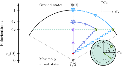
Figure 1: Bloch sphere representation of the refrigeration dynamics. Standard cooling processes may be regarded as a swap between the initial state of the system with polarization $\varepsilon_{\textsl{s}}(0)$ (red dot) and an incoherent virtual qubit with polarization $\varepsilon_{\textsl{v}}$ (purple star). Adding coherence, characterized by the parameter $\gamma$, to the virtual qubit moves the state closer to the surface of the sphere while keeping its polarization constant (green star). Better cooling is achieved by unitarily rotating the state back to the energy axis (violet star). Ground state cooling (blue star) is, in principle, possible for maximum coherence $(\gamma=1)$, when the state reaches the surface of the sphere. The inset shows the coordinates of the virtual qubit, radius $\hat{\gamma}=\gamma\sqrt{1-\varepsilon_{\textsl{v}}^{2}}/2$ and angle $\alpha$, viewed from above.

From a physical point of view, for long times (or large cycle number), the cooling dynamics effectively exchanges the initial state $\rho_{\textsl{s}}(0)$ of the system qubit with the asymptotic state $\mathcal{R}_{\infty}[\rho_{\textsl{s}}(0)]$. Mathematically, this operation may be regarded as a full swap nie02 between initial and final states. We shall use this observation to operationally define the virtual qubit. Virtual subsystems are often determined by specifying a given factorization of the Hilbert space zan01 ; zan04 ; lid13 ; kni99 ; kri05 ; kni06 ; dua97 ; zan97 ; lid98 ; zan03 ; choi06 ; blu08 ; dua97 ; dur03 ; cai09 ; cai10 ; pop05 ; kab20 ; car21 , see also Ref. com . However, any purification dynamics may be viewed as a generalized swap process between the system qubit and a sufficiently pure virtual qubit tic14 . By reversing this argument, we can identify the virtual qubit with the steady state $\rho_{\textsl{v}}=\mathcal{R}_{\infty}[\rho_{\textsl{s}}(0)]$. The virtual qubit is thus encoded in the refrigeration superoperator, hence providing an operational method to determine it for an arbitrary cooling process. This is nontrivial, since usually the virtual qubit does not coincide with any original qubit of the problem, but is given by two levels in a multidimensional system. For a continuous-time cooling process, the virtual qubit may correspond to a two-level subsystem of the two heat reservoirs considered as a composite entity bru12 ; ven13 ; cor13 ; boh15 ; mit15 ; sil16 ; man17 ; erk17 ; du18 ; mit19 ; rig21 , while it might be given by two levels of the ancilla qubit system for a discrete-time heat-bath algorithmic cooling process (see example below). Common (incoherent) cooling schemes are associated with incoherent virtual qubits.

We next analyze the cooling advantage of a coherent virtual qubit with linearly superposed energy states. To this end, it is convenient to describe the refrigeration dynamics using a Bloch sphere representation of the qubit, defined by writing any density operator as $\rho=(I+\sum_{i}i\sigma_{i})/2$, with $i=(x,y,z)$ and $\sum_{i}i^{2}\leq 1$ ben06 . The process initially starts with the thermal state with coordinates $(0,0,\varepsilon_{\textsl{s}}(0))$ (red dot in Fig. 1). Standard cooling protocols proceed along the (energy) $z$-axis kos14 , corresponding to an incoherent virtual qubit, $\rho_{\textsl{v}}=(I+\varepsilon_{\textsl{v}}\sigma_{z})/2$, with polarization $\varepsilon_{\textsl{v}}>\varepsilon_{\textsl{s}}(0)$. After (infinitely) many cooling cycles, the system ends in the refrigerated state $(0,0,\varepsilon_{\textsl{v}})$ (purple star in Fig. 1). The lowest possible temperature in this framework is $T_{\text{min}}=T\omega/\Omega$, where $T$ is the temperature of the (hot) bath and $\Omega$ is the largest energy of the machine all11 ; ree14 ; cli19 ; cli19a . So far, strategies to improve this incoherent cooling limit amount to decrease the temperature of the virtual qubit, or, equivalently, increase its polarization.

We here explore another method based on a coherent virtual qubit, which we parametrize as

$$\rho_{\textsl{v}}=\frac{1}{2}\begin{pmatrix}1+\varepsilon_{\textsl{v}}&\gamma\mathrm{e}^{-\mathrm{i}\alpha}\sqrt{1-\varepsilon_{\textsl{v}}^{2}}\\ \gamma\mathrm{e}^{\mathrm{i}\alpha}\sqrt{1-\varepsilon_{\textsl{v}}^{2}}&1-\varepsilon_{\textsl{v}}\end{pmatrix},$$ (1)

where $0\leq\gamma\leq 1$ is a measure of quantum coherence, and $\alpha$ defines the direction of $\sigma_{\alpha}=\cos(\alpha)\sigma_{x}+\sin(\alpha)\sigma_{y}$. The plane $\sigma_{z}\crossproduct\sigma_{\alpha}$ is then perpendicular to the $\sigma_{x}\crossproduct\sigma_{y}$ plane. The Bloch coordinates of the virtual qubit are now $(x_{\textsl{v}}+\mathrm{i}y_{\textsl{v}}=\gamma\mathrm{e}^{\mathrm{i}\alpha}\sqrt{1-\varepsilon_{\textsl{v}}^{2}},z_{\textsl{v}}=\varepsilon_{\textsl{v}})$ (green star in Fig. 1). Endowing the virtual qubit with coherence $\gamma$ (with fixed polarization $\varepsilon_{\textsl{v}}$) increases its purity, moving the virtual state away from the energy axis and closer to the surface of the Bloch sphere. After many cooling cycles, the system state will approach the coherent virtual state (wavy lines). Lower system qubit temperatures may then be achieved by rotating the system state back to the energy basis at the end of the coherent cooling process (violet star in Fig. 1). For this single additional step, we only consider unitary operations that do not change the purity. This is justified because any other resource that may further increase purity could have been used to achieve a higher polarization $\varepsilon_{\textsl{v}}$ in the first place com1 .

Coherent cooling limits. The maximum achievable system polarization using a coherent virtual qubit is

$$\varepsilon_{\star}(\gamma)=\sqrt{\varepsilon_{\textsl{v}}^{2}+(1-\varepsilon_{\textsl{v}}^{2})\gamma^{2}},$$ (2)

given by the eigenvalues of the coherent virtual qubit state (violet star in Fig. 1). This coherent cooling limit neither depends on the details of the cooling protocol nor on the specific mechanism creating the coherent virtual qubit; it hence appears to be universal. The coherent bound $\varepsilon_{\star}$ generally exceeds the incoherent bound $\varepsilon_{\textsl{v}}$. The unitary transformation realizing the appropriate rotation at the end of the coherent cooling sequence should be orthogonal to $\sigma_{\alpha}$, with an angle that depends on $\gamma$. It is explicitly given by $V=\exp(\mathrm{i}\chi(\gamma)\,\sigma_{\perp}(\alpha)/2)$ with $\sigma_{\perp}(\alpha)=-\sin(\alpha)\sigma_{x}+\cos(\alpha)\sigma_{y}$ and $\chi(\gamma)=\arccos[\varepsilon_{\textsl{v}}/\varepsilon_{\star}(\gamma)]$ (violet line in Fig. 1). The standard refrigeration bound, $\varepsilon_{\star}(0)=\varepsilon_{\textsl{v}}$, is recovered in the absence of coherence, $\gamma=0$. In the opposite limit of maximum coherence, $\gamma=1$, ground state cooling, $\varepsilon_{\star}(1)=1$, is in principle possible, with a rotation angle $\chi(1)=\arccos(\varepsilon_{\textsl{v}})$ (blue line in Fig. 1). We emphasize that this result does not contradict the unattainability principle of the third law of thermodynamics bel04 , since it presupposes perfect knowledge of the values of $\gamma$ and $\alpha$, as well as a perfect implementation of the unitary rotation. Both are not possible in any realistic experiment. This is reminiscent of the (practical) impossibility of violating the second law of thermodynamics by reversing all the velocities of a system (Loschmidt’s reversibility paradox) bel04 , since this would require perfect control over the system.

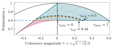
Figure 2: Improved cooling with incomplete knowledge of the amount of quantum coherence of the virtual qubit. Enhanced cooling, $\varepsilon\geq\varepsilon_{\textsl{v}}$, can be achieved even if the amount of coherence $\gamma$ is only known to be in an interval $[\gamma_{\min},\gamma_{\max}]$, when the virtual qubit state is such that $\gamma_{\inf}<\gamma$, Eq. (5) (blue shaded area). This even holds when the value of $\gamma$ is completely unknown ($\gamma_{\min}=0$ and $\gamma_{\max}=1$). This is, in particular, the case, for the middle point, $\gamma_{\text{avg}}$, of the confidence interval.

In practice, the parameters $\gamma$ and $\alpha$ are usually not known precisely. Yet, improved cooling might still be achieved, as we will now discuss com4 . Let us distinguish between the parameters $(\gamma,\alpha)$ of the given coherent virtual state and the parameters $(\gamma_{\text{rot}},\alpha_{\text{rot}})$ of the implemented rotation $V$. We assume, for simplicity, that $\alpha=\alpha_{\text{rot}}$ is fixed and that $\gamma$ is uniformly distributed in a confidence interval $[\gamma_{\min},\gamma_{\max}]$ (the case of an unknown $\alpha$ is examined in the Supplemental Material sm ). We first determine the maximal value $\gamma_{\text{rot}}$ that still yields improved cooling given an amount of coherence $\gamma$. There are three regions for which this is possible. For $1/2\leq\gamma$, every choice of $\gamma_{\text{rot}}$ leads to improved cooling, irrespective of the value of $\varepsilon_{\textsl{v}}$. For $\gamma\leq 1/2$, increased refrigeration will happen for all values of $\gamma_{\text{rot}}$, provided that the polarization obeys $\varepsilon_{\textsl{v}}\leq\gamma/(1-\gamma)$. Finally, for $\varepsilon_{\textsl{v}}>\gamma/(1-\gamma)$, enhanced cooling will occur for

$$\gamma_{\text{rot}}\leq\frac{2\varepsilon_{\textsl{v}}^{2}\gamma}{\varepsilon_{\textsl{v}}^{2}-\gamma^{2}(1-\varepsilon_{\textsl{v}}^{2})}.$$ (3)

The maximum achievable system polarization depends on the rotation angle $\chi(\gamma_{\text{rot}})>0$, and is given by

$$\varepsilon_{\chi(\gamma_{\text{rot}})}=\frac{\varepsilon_{\textsl{v}}^{2}+\gamma\gamma_{\text{rot}}(1-\varepsilon_{\textsl{v}}^{2})}{\sqrt{\gamma_{\text{rot}}^{2}+\varepsilon_{\textsl{v}}^{2}(1-\gamma_{\text{rot}}^{2})}}.$$ (4)

When $\gamma_{\text{rot}}\leq\gamma_{\min}$, enhanced cooling is possible for all $\gamma>\gamma_{\min}$. The highest possible system polarization, $\varepsilon_{\chi(\gamma_{\max})}$, is obtained for $\gamma=\gamma_{\max}$. Care is required when $\gamma_{\text{rot}}>\gamma_{\min}$, since a large enough rotation of a state with small enough coherence $\gamma$ may result in heating (red shaded area in Fig. 2). Equating $\varepsilon_{\chi(\gamma_{\text{rot}})}$, Eq. (4), to $\varepsilon_{\textsl{v}}$, and solving for $\gamma$ yields a second lower bound for the coherence $\gamma$, that is different from $\gamma_{\min}$,

$$\gamma_{\inf}(\gamma_{\text{rot}})=\varepsilon_{\textsl{v}}\frac{\sqrt{\varepsilon_{\textsl{v}}^{2}+\gamma_{\text{rot}}^{2}(1-\varepsilon_{\textsl{v}}^{2})}}{\gamma_{\text{rot}}(1-\varepsilon_{\textsl{v}}^{2})}-\frac{\varepsilon_{\textsl{v}}^{2}}{\gamma_{\text{rot}}(1-\varepsilon_{\textsl{v}}^{2})},$$ (5)

so that heating is avoided (Fig. 2). Best refrigeration is found for $\gamma=\gamma_{\max}$ and is again given by Eq. (4) com2 . We note that, for $\gamma_{\text{rot}}\leq\gamma_{\max}$, taking the unknown value of $\gamma$ as the middle point of the confidence interval, $\gamma_{\text{avg}}=(\gamma_{\min}+\gamma_{\max})/2$, always leads to improved cooling, since $\gamma_{\text{avg}}>\gamma_{\inf}$ (Fig. 2). Interestingly, this result even holds when the amount of coherence $\gamma$ is completely unknown ($\gamma_{\min}=0$ and $\gamma_{\max}=1$). The above equations fully determine the improved quantum cooling domain (blue area in Fig. 2). They establish the robustness of the proposed scheme against experimental imperfections.

Application to heat-bath algorithmic cooling. The above analysis of the cooling advantage of coherent virtual qubits is completely general. We next apply it to heat-bath algorithmic cooling boy02 ; par16 ; fer04 ; sch05 ; sch07 ; rem07 ; kay07 ; bra14 ; rai15 ; rod16 ; rai19 ; sol22 that has recently been implemented experimentally bau05 ; rya08 ; par15 ; ata16 ; zai21 . Its smallest version is made of three qubits: one system (target) qubit with state $\rho_{\textsl{s}}(n)=\rho_{1}(n)$, to be cooled, and two ancilla (reset) qubits with separable states $\rho_{\textsl{a}}=\rho_{2}\otimes\rho_{3}$. The cooling algorithm consists of (i) a compression step during which a unitary $U$ implements the transition $\outerproduct{011}{100}+\text{h.c.}$, pumping heat out of the target qubit and into the two reset qubits, followed by (ii) a refresh step that thermalizes the reset qubits back to their initial bath polarization $\varepsilon_{2}$ and $\varepsilon_{3}$ (Fig. 3a). The corresponding quantum channels, that operate on the three-qubit ensemble, are $\mathcal{U}(\rho)=U\rho U^{\dagger}$ for the cooling part and $\mathcal{E}(\rho)=\rho\otimes\rho_{2}\otimes\rho_{3}$ for the expansion part. In the limit of many cooling cycles, the target qubit reaches the asymptotic polarization $\varepsilon_{1}(\infty)$. This operation may be understood as a full swap between the initial state of the target qubit and an incoherent virtual qubit consisting of the two states $\ket{0_{2}0_{3}}$ and $\ket{1_{2}1_{3}}$. The standard cooling limit is here determined by the polarization of the incoherent virtual qubit, $\varepsilon_{\textsl{v}}(\varepsilon_{2},\varepsilon_{3})=(\varepsilon_{2}+\varepsilon_{3})/(1+\varepsilon_{2}\varepsilon_{3})$ sol22 . For simplicity, we will set $\varepsilon_{2}=\varepsilon_{3}=\varepsilon_{\textsl{a}}$ in the remainder.

We now introduce a coherent extension of this cooling algorithm such that $\mathcal{E}^{c}(\rho)=\rho\otimes\rho_{23}$, where $\rho_{23}$ is a nonseparable state. Such state may, for example, be simply generated by considering interacting reset qubits (see detailed discussion below), or by directly entangling them har22 . The dynamics of the system qubit is then described by the coherent refrigeration process

$$\rho_{1}(n)=\mathcal{R}^{c}_{n}(\rho_{1}(0))=({\tr_{23}}\circ\mathcal{U}\circ\mathcal{E}^{c})^{n}(\rho_{1}(0)),$$ (6)

after $n$ cycles. The transformation (6) both cools the target qubit and transfers coherence from the virtual qubit to the target qubit. In the asymptotic limit, the coherent refrigeration superoperator takes the form of a swap with a coherent virtual qubit, $\mathcal{R}^{c}_{\infty}(\cdot)=\tr_{\textsl{v}}S(\cdot\otimes\rho_{\textsl{v}})S^{\dagger}$, with swap operator $S$ nie02 . We parametrize the coherence of the virtual qubit by the matrix elements, $\matrixelement{00}{\rho_{23}}{11}=({\xi}/{4})\mathrm{e}^{-\mathrm{i}\alpha}(1-\varepsilon_{\textsl{a}}^{2})$, ($0\leq\xi\leq 1$), which implies $\matrixelement{0}{\rho_{\textsl{v}}}{1}=({\gamma}/{2})\mathrm{e}^{-\mathrm{i}\alpha}\sqrt{1-\varepsilon_{\textsl{v}}^{2}}$, with $\gamma=\varepsilon_{\textsl{v}}\xi$. In order to achieve a fair comparison between coherent and incoherent cooling strategies, we analyze the effect of coherence while fixing the polarization of the virtual qubit so that it is the same as that of the incoherent one. In view of Eq. (2), the maximum achievable target polarization of this coherent algorithmic cooling scheme is then $\varepsilon_{\star}=\varepsilon_{\textsl{v}}\sqrt{2-\varepsilon_{\textsl{v}}^{2}}\geq\varepsilon_{\textsl{v}}$, for $\xi=1$, which clearly exceeds the current incoherent cooling limit $\varepsilon_{\textsl{v}}$.

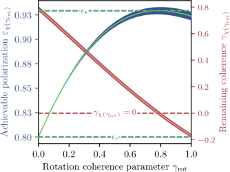
Figure 3: Achievable target polarization $\varepsilon_{\chi(\gamma_{\text{rot}})}$, Eq. (4), (green) after a unitary rotation parametrized by the coherence parameter $\gamma_{\text{rot}}$ for a realistic heat-bath algorithmic cooling protocol using nitrogen-vacancy (NV) centers in diamond. The coherent virtual qubit has polarization $\varepsilon_{\textsl{v}}=0.8$. Maximum polarization $\varepsilon_{\star}$ is reached for $\gamma_{\text{rot}}\sim 0.79$, a value for which the remaining coherence of the virtual qubit, $\gamma_{\chi(\gamma_{\text{rot}})}$, (pink) vanishes; the blue and red shaded areas represent the respective confidence intervals of $\varepsilon_{\chi(\gamma_{\text{rot}})}$ and $\gamma_{\chi(\gamma_{\text{rot}})}$.

As an illustration, we examine the achievable polarization $\varepsilon_{\chi(\gamma_{\text{rot}})}$, Eq. (4), as a function of $\gamma_{\text{rot}}$ for a realistic confidence interval available in experiments using nitrogen-vacancy (NV) centers in diamond zai21 . The two reset qubits are here two carbon ¹³C nuclear spins that are coupled to the central electron spin of the NV center zai21 . We consider a maximally coherent virtual qubit ($\xi=1$) with polarization $\varepsilon_{\textsl{v}}=\gamma=0.8$ prepared with $97.6\%$ fidelity. We accordingly have $\gamma_{\min}=0.78$ and $\gamma_{\max}=0.8$. Figure 3 displays the tradeoff between the achievable polarization $\varepsilon_{\chi(\gamma_{\text{rot}})}$ (green) and the remaining coherence $\gamma_{\chi(\gamma_{\text{rot}})}$ (pink) after the final unitary rotation (the blue and red shaded areas represent the corresponding confidence intervals). Maximal polarization of $\varepsilon_{\chi(\gamma_{\text{rot}})}\sim 0.93$ is attained for $\gamma_{\text{rot}}\sim 0.79$, where the remaining coherence vanishes. This value significantly exceeds the incoherent cooling bound $\varepsilon_{\textsl{v}}=0.8$ and saturates the coherent refrigeration bound $\varepsilon_{\star}$. For a rotation angle larger than the optimal value, the achievable polarization decreases; this overshoot corresponds to the red shaded area on the left-hand side of Fig. 2.

Roadmap to enhanced quantum cooling. The above results outline a generic strategy to improve existing incoherent cooling schemes which consists of three steps: (i) determining the usually nontrivial incoherent virtual qubit from the steady-state limit of the incoherent refrigerator superoperator, (ii) endowing it with quantum coherence, which can be done passively by choosing an appropriate set of controlled observables, and (iii) implementing an appropriate unitary rotation on the system qubit at the end of the cooling sequence to bring it back to the (incoherent) energy axis. The first step holds for any cooling protocol, and allows one to identify the incoherent virtual qubit from the knowledge of the incoherent cooling process. The second step will in general depend on the considered cooling method. However, the heat-bath algorithmic cooling example analyzed above provides valuable general clues. In the latter case, the coherent virtual qubit may indeed be easily generated by considering interacting reset qubits, for instance, via a transverse-Ising type coupling of the form $H_{23}=-(\omega/4)(\sigma^{z}_{2}+\sigma^{z}_{3})+g\sigma^{x}_{2}\sigma^{x}_{3}-g\sigma^{y}_{2}\sigma^{y}_{3}$ with coupling constant $g$ (the corresponding coherent cooling process is simulated in the Supplemental Material sm ); the standard heat-bath algorithmic cooling protocol uses noninteracting reset qubits with $g=0$ bau05 ; rya08 ; par15 ; ata16 ; zai21 . The system will then exhibit quantum coherence in the local energy bases of each reset qubit when the global two-qubit state is an (incoherent) thermal Gibbs state, which, in turn, will make the virtual qubit coherent. This follows from the fact that quantum coherence generally depends on the choice of a basis in Hilbert space nie02 , which is reminiscent of the finding that the tensor-product structure of the Hilbert space generally depends on the choice of a set of observables zan04 . The same mechanism should be applicable to more complicated refrigeration schemes; it is important to realize that all the other parts of the cooling algorithm are not modified. Finally, the last step only entails a single unitary rotation of the system qubit after completion of the coherent refrigeration process.

Conclusions. The current experimental development of quantum applications seems to mostly rely on nonquantum cooling schemes, without fully harnessing the power of coherent refrigeration. By extending the concept of virtual qubits to coherent virtual qubits, and further showing that they may be operationally determined from the asymptotic limit of any refrigeration superoperator, we have shown that it is possible to cool beyond existing incoherent refrigeration bounds. We have concretely obtained generic coherent cooling bounds that are independent of the considered setup. Quantum coherence thus appears as a useful physical resource in this context. Remarkably, enhanced cooling is feasible, even if the amount of coherence is not exactly known. This makes this quantum refrigeration scheme robust for experimental implementations. In the present approach, virtual qubits function as a reservoir of coherence, which is different from dynamically generated coherence that has been found to assist cooling in some instances, such as single-shot cooling mit15 . We have moreover introduced a coherent heat-bath algorithmic cooling protocol and specified its enhanced cooling limit. Our findings provide a general framework to investigate the properties of coherent refrigeration processes and additionally improve the performance of existing incoherent cooling protocols.

Acknowledgments. We acknowledge the financial support by the DFG (FOR 2724), DFG (509457256), BMBF (Grant No. 16KIS1590K), EU GRK2642, AMADEUS, QIA, Max Planck Society, and the Baden-Württemberg Foundation. R. R. S. further acknowledges fruitful discussions with R. Laflamme and N. A. Rodriguez-Briones, and the financial support by DAAD (research grant Bi-nationally Supervised Doctoral Degrees/Cotutelle, 57507869) and from CNPq (141797/2019-3).

Supplemental Material

The Supplemental Material contains details about (I) the dynamics of the target qubit for the minimal heat-bath algorithmic cooling model with a coherent virtual qubit, (II) the generation of the coherent virtual qubit, as well as (III) the simulation of the generalized protocol, (IV) the determination of the cooling regions for the case of an unknown coherence phase $\alpha$, (V) an analysis of the thermodynamic performance of the coherent protocol, and (VI) a comparison with heat-bath algorithmic cooling with multiple reset qubits.

Appendix A Analytical solution of the target qubit dynamics in the natural representation

We here provide the analytical solution of the target qubit dynamics for the minimal heat-bath algorithmic cooling model with a coherent virtual qubit discussed in the main text. To this end, we first introduce the natural representation (vectorization map) wat18 , also sometimes referred to as Liouville space representation gya20 , used to reach the result.

A.1 Vectorization method

We introduce the vectorization transformations that map states into column matrices and quantum channels into matrix operators, acting on the columns. To set the notation, we define vectorization on states as

$$\operatorname{vec}\colon\rho\mapsto\vec{\rho}.$$ (S1)

In the qubit case, the central Hilbert space from which the quantum dynamics are constructed is $\mathbf{H}=\mathbb{C}^{2}$. Thus, the density matrix of a state is represented by an element of $\mathbb{M}_{\mathbb{C}}^{2\times 2}$, that is, by 2-by-2 matrices with complex entries that are Hermitian and positive semidefinite. In terms of its elements, a density matrix is mapped by $\operatorname{vec}$ by stacking its columns into a single one, such as in

$$\frac{1}{2}\begin{pmatrix}1+\varepsilon&x+\mathrm{i}y\\ x-\mathrm{i}y&1-\varepsilon\end{pmatrix}\xmapsto{\operatorname{vec}}\frac{1}{2}\begin{pmatrix}1+\varepsilon\\ x-\mathrm{i}y\\ x+\mathrm{i}y\\ 1-\varepsilon\end{pmatrix},$$ (S2)

where $\mathbb{M}_{\mathbb{C}}^{2\times 2}\stackrel{{\scriptstyle\operatorname{vec}}}{{\cong}}\mathbb{M}_{\mathbb{C}}^{1\times 4}=\mathbb{C}^{4}$. We call Liouville space the resulting column matrix space.

The second vectorization mapping, also known as the natural representation of quantum maps $\Phi$ wat18 , is induced from the following compatibility condition:

$$\Phi_{\mathcal{K}}\vec{\rho}=\operatorname{vec}[\mathcal{K}(\rho)],$$ (S3)

where $\mathcal{K}$ is a quantum channel, such as the one defined by the operator sum representation with Kraus operators $K_{\mu}$ as $\mathcal{K}(\rho)=\sum_{\mu}K_{\mu}\rho K_{\mu}^{\dagger}$. In words, the compatibility condition is the statement that there exists $\Phi_{\mathcal{K}}$ such that it maps the vectorized input state to the vectorization of the output of $\mathcal{K}$.

The solution to the compatibility condition in these variables is

$$\Phi_{\mathcal{K}}=\sum_{\mu}K_{\mu}\otimes K_{\mu}^{*}.$$ (S4)

As such, a map $\Phi_{\mathcal{K}}$ is a matrix element of $\mathbb{M}_{\mathbb{C}}^{4\times 4}$ that allows rewriting the operator sum representation of $\mathcal{K}$ as simple matrix multiplication.

A.2 Solution for target qubit evolution

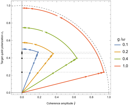
Figure S1: Bloch sphere representation of the evolution of the polarization $\varepsilon_{1}$ of the target qubit as the number of cycle number $n$ (arrowheads) is increased, for various values of the ratio $g/\omega$. The reset qubits are here assumed to interact via a transverse-field Ising Hamiltonian of the form $H=-\frac{\omega}{4}(\sigma^{z}_{2}+\sigma^{z}_{3})+g\sigma^{x}_{2}\sigma^{x}_{3}-g\sigma^{y}_{2}\sigma^{y}_{3}$, with frequency $\omega$ and coupling constant $g$. Both the polarization and the amount of coherence increase with the number of cycles. The inverse temperature is taken to be $\beta=1.09/\omega$. Black dots represent the polarization of the corresponding incoherent virtual qubit we compare to.

The dynamical map $\mathcal{R}_{n}$ for heat-bath algorithmic cooling is Markovian, and thus at arbitrary cycle number $n$, it contains every necessary information of the qubit evolution. Its nonzero elements are sol22

$$(\Phi_{\mathcal{R}}^{n})_{11}={} \frac{(1-\varepsilon_{2})(1-\varepsilon_{3})}{2(1+\varepsilon_{2}\varepsilon_{3})}\frac{(1-\varepsilon_{2}\varepsilon_{3})^{n}}{2^{n}}+\frac{(1+\varepsilon_{2})(1+\varepsilon_{3})}{2(1+\varepsilon_{2}\varepsilon_{3})}$$ (S5)

$$(\Phi_{\mathcal{R}}^{n})_{21}={} \bigg{[}(\varepsilon_{2}+\varepsilon_{3})(\varepsilon_{2}\varepsilon_{3}-1)$$

$$-\big{[}(\varepsilon_{2}+\varepsilon_{3})(1-\varepsilon_{2}\varepsilon_{3})-n(1-\varepsilon_{2})(1-\varepsilon_{3})(1+\varepsilon_{2}\varepsilon_{3})\big{]}\frac{(1-\varepsilon_{2}\varepsilon_{3})^{n}}{2^{n}}\bigg{]}\frac{\mathrm{e}^{\mathrm{i}\alpha^{\prime}}\xi\sqrt{1-\varepsilon_{2}^{2}}\sqrt{1-\varepsilon_{3}^{2}}}{2(\varepsilon_{2}\varepsilon_{3}-1)(1+\varepsilon_{2}\varepsilon_{3})^{2}}.$$ (S6)

These are two elements that will help define the virtual qubit $\rho_{\textsl{v}}$ asymptotically as $n\to\infty$. As such, the rest of the matrix is

$$\Phi_{\mathcal{R}}^{n}=\begin{pmatrix}(\Phi_{\mathcal{R}}^{n})_{11}&0&0&(\Phi_{\mathcal{R}}^{n})_{11}\\ (\Phi_{\mathcal{R}}^{n})_{21}&(\Phi_{\mathcal{R}}^{n})_{22}&0&(\Phi_{\mathcal{R}}^{n})_{21}\\ (\Phi_{\mathcal{R}}^{n})_{21}^{*}&0&(\Phi_{\mathcal{R}}^{n})_{33}&(\Phi_{\mathcal{R}}^{n})_{21}^{*}\\ 1-(\Phi_{\mathcal{R}}^{n})_{11}&0&0&1-(\Phi_{\mathcal{R}}^{n})_{11}\end{pmatrix}.$$ (S7)

The remaining elements $(\Phi_{\mathcal{R}}^{n})_{22}$ and $(\Phi_{\mathcal{R}}^{n})_{33}$ are explicitly given by

$$(\Phi_{\mathcal{R}}^{n})_{22}=(\Phi_{\mathcal{R}}^{n})_{33}=\frac{(1-\varepsilon_{2}\varepsilon_{3})^{n}}{2^{n}}.$$ (S8)

These elements carry information of initial coherences but vanish asymptotically. However, in the transient dynamics, there are cross contributions from the coherence that was input into the target and the coherence that is yet to come. The full evolution of the target qubit is accordingly

$${\bra{0}}{\rho_{1}(n)}{\ket{0}} =\frac{(\varepsilon_{1}\varepsilon_{2}\varepsilon_{3}+\varepsilon_{1}-\varepsilon_{2}-\varepsilon_{3})}{2(1+\varepsilon_{2}\varepsilon_{3})}\frac{(1-\varepsilon_{2}\varepsilon_{3})^{n}}{2^{n}}+\frac{(1+\varepsilon_{2})(1+\varepsilon_{3})}{2(1+\varepsilon_{2}\varepsilon_{3})}$$ (S9)

$${\bra{1}}{\rho_{1}(n)}{\ket{0}} =\begin{multlined}\left[\frac{(\varepsilon_{2}+\varepsilon_{3})}{(1+\varepsilon_{2}\varepsilon_{3})}-\left(\frac{(\varepsilon_{2}+\varepsilon_{3})}{(1+\varepsilon_{2}\varepsilon_{3})}-\frac{n}{1-\varepsilon_{2}\varepsilon_{3}}(\varepsilon_{1}\varepsilon_{2}\varepsilon_{3}+\varepsilon_{1}-\varepsilon_{2}-\varepsilon_{3})\right)\frac{(1-\varepsilon_{2}\varepsilon_{3})^{n}}{2^{n}}\right]\frac{\mathrm{e}^{\mathrm{i}\alpha^{\prime}}\xi\sqrt{1-\varepsilon_{2}^{2}}\sqrt{1-\varepsilon_{3}^{2}}}{2(1+\varepsilon_{2}\varepsilon_{3})}\\ +\frac{\chi\sqrt{1-\varepsilon_{1}^{2}}}{2}\frac{(1-\varepsilon_{2}\varepsilon_{3})^{n}}{2^{n}},\end{multlined}\left[\frac{(\varepsilon_{2}+\varepsilon_{3})}{(1+\varepsilon_{2}\varepsilon_{3})}-\left(\frac{(\varepsilon_{2}+\varepsilon_{3})}{(1+\varepsilon_{2}\varepsilon_{3})}-\frac{n}{1-\varepsilon_{2}\varepsilon_{3}}(\varepsilon_{1}\varepsilon_{2}\varepsilon_{3}+\varepsilon_{1}-\varepsilon_{2}-\varepsilon_{3})\right)\frac{(1-\varepsilon_{2}\varepsilon_{3})^{n}}{2^{n}}\right]\frac{\mathrm{e}^{\mathrm{i}\alpha^{\prime}}\xi\sqrt{1-\varepsilon_{2}^{2}}\sqrt{1-\varepsilon_{3}^{2}}}{2(1+\varepsilon_{2}\varepsilon_{3})}\\ +\frac{\chi\sqrt{1-\varepsilon_{1}^{2}}}{2}\frac{(1-\varepsilon_{2}\varepsilon_{3})^{n}}{2^{n}},$$ (S12)

where we here consider the presence of an initially coherent target qubit with coherence $\chi=|\chi|\mathrm{e}^{-\mathrm{i}\arg(\chi)}$ parametrized as usual in the rest of the paper. This contribution comes from $(\Phi_{\mathcal{R}}^{n})_{22}$, and vanishes asymptotically as it is replaced by the virtual qubit coherence.

Appendix B Generation of a coherent virtual qubit

In the case of the three-qubit heat-bath algorithmic cooling example discussed in the main text, a coherent virtual qubit could be simply and naturally created by considering two interacting reset qubits, instead of the two noninteracting reset qubits employed in the standard, incoherent heat-bath algorithmic cooling protocol (coherence could, of course, also be engineered artificially, but this would be more costly). For instance, the thermal state of a two-spin transverse-field Ising model with Hamiltonian, $H=-\frac{\omega}{4}(\sigma^{z}_{2}+\sigma^{z}_{3})+g\sigma^{x}_{2}\sigma^{x}_{3}-g\sigma^{y}_{2}\sigma^{y}_{3}$, naturally contains coherences with respect to each qubit’s local energy bases. As a result, the corresponding virtual qubit also exhibits coherences that scale with inverse temperature $\beta$ and coupling strength $g$ as $\gamma\sim g\tanh{(\beta\sqrt{g^{2}+\omega^{2}})}$.

Figure S1 shows the Bloch sphere representation of the evolution of the polarization $\varepsilon_{1}$ of the target qubit as the number of cycle number $n$ (dots) is increased, for various values of the ratio $g/\omega$. This figure is a concrete illustration (for each coupling strength $g$) of the schematic diagram shown in Fig. 1 of the main text, where we compare the asymptotic state with its corresponding incoherent virtual qubit state, lying on the $y$-axis. We note that both the polarization and the amount of coherence increase with the number of cycles, indicating that the protocol is capable of transporting quantum coherence from each virtual qubit to the target qubit at the same time that the target qubit is cooled. The surface of the Bloch sphere, corresponding to maximal target coherence, is almost reached for $g/\omega=1$.

Appendix C Simulation of the coherent cooling protocol

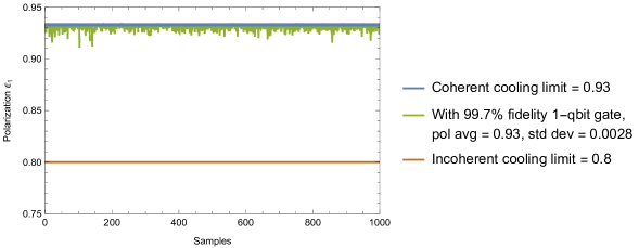
Figure S2: Target polarization for coherent and incoherent cooling protocols with realistic experimental parameters. Reset polarizations are set to $\varepsilon_{\textrm{res}}=0.5$ corresponding to an incoherent cooling limit of $\varepsilon^{\text{inc}}_{\textrm{lim}}=0.8$ (brown line). (1) Green: target polarization achieved with a 1-qubit unitary gate with fidelity $99.7\%$ applied once to the target qubit; it is close to the maximal achievable coherent polarization bound $\varepsilon^{\text{coh}}_{\textrm{max}}=0.93$ (blue line).

In this section, we present a numerical simulation of the generalized heat-bath algorithmic cooling scheme with a coherent virtual qubit, using realistic experimental parameters. The nontrivial advantage of the suggested protocol is that it is capable of transporting the coherences from each virtual qubit to the target qubit at the same time that the target qubit is cooled. This results in a target qubit which is also coherent in the steady state, and therefore a single unitary gate on the target qubit is enough to take advantage of all available coherences – and achieve better cooling.

Figure S2 shows the outcome of numerical simulations based on our available NV center gate fidelities for 1-qubit gates $\mathcal{V}$ (99.6$\%$ to 99.8$\%$); we assume 100$\%$ fidelity for the implementation of the refrigeration channel $\mathcal{R}$ in order to better highlight the effect the different gate fidelities. We observe that our protocol (green, see also Fig. S3) gets very close to the coherent cooling limit $\varepsilon^{\text{coh}}_{\textrm{max}}=0.93$ (blue), which clearly surpasses the incoherent cooling limit $\varepsilon^{\text{inc}}_{\textrm{lim}}=0.8$ (brown).

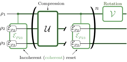
Figure S3: Minimal heat-bath algorithmic cooling application. Wire diagram for an $n$-iteration of the incoherent algorithm (black) and the coherent extension (green), followed by the polarization-enhancing rotation, $\mathcal{V}(\cdot)=V\cdot V^{\dagger}$. The fidelity of the two-qubit gate that comprises part of the compression unitary U, as well as the particular form of this unitary, determine the coherence confidence interval discussed in the main text.

Appendix D Cooling with unknown coherence phase

We next consider the situation where the coherence angle $\alpha$ is known to be in a confidence interval $\alpha_{\min}\leq\alpha\leq\alpha_{\max}$, and determine the associated cooling domains. This random unitary case samples axes of rotations distributed over the $\sigma_{x}\crossproduct\sigma_{y}$ plane. The cooling regions are found by integrating the polarization value of the rotated ensemble of states,

$$\varepsilon_{\chi(\gamma_{\text{rot}})}=\gamma\sqrt{1-\varepsilon_{\textsl{v}}^{2}}\sin(\alpha-\alpha_{\text{rot}})\sin(\chi(\gamma_{\text{rot}}))+\varepsilon_{\textsl{v}}\cos(\chi(\gamma_{\text{rot}})),$$ (S13)

over the surface defined by $\alpha$ and $\alpha_{\text{rot}}$:

$$\begin{split}\overline{\varepsilon_{\chi(\gamma_{\text{rot}})}}={}&\frac{1}{\Delta\alpha^{2}}\int_{\alpha_{\min}}^{\alpha_{\max}}\int_{\alpha_{\min}-\pi/2}^{\alpha_{\max}-\pi/2}\differential{\alpha}\differential{\alpha_{\text{rot}}}\varepsilon_{\chi(\gamma_{\text{rot}})}\\ ={}&\frac{2\gamma\gamma_{\text{rot}}(\varepsilon_{\textsl{v}}^{2}-1)\cos(\Delta\alpha)-2\gamma\gamma_{\text{rot}}(\varepsilon_{\textsl{v}}^{2}-1)+\Delta\alpha^{2}\varepsilon_{\textsl{v}}^{2}}{\varepsilon_{\textsl{v}}^{2}-(\varepsilon_{\textsl{v}}^{2}-1)\gamma_{\text{rot}}^{2}}\end{split}.$$ (S14)

In Fig. S4(a), we show the parameter space for average achievable polarization, $\overline{\varepsilon_{\chi(\gamma_{\text{rot}})}}$, with corresponding cooling (blue) and heating (red) regions. We again fix the initial polarization at $\varepsilon_{\textsl{v}}=0.8$, as in the main text. We observe a large cooling region (bottom part of the figure) for various values of $\Delta\alpha$ and of $\gamma_{\text{rot}}/\gamma$. Incomplete knowledge of the coherence phase $(\Delta\alpha=2\pi)$ does not lead to average cooling, in contrast to what happens for incomplete knowledge of the coherence parameter $\gamma$ discussed in the main text. Enhanced average cooling is achieved for all $\gamma_{\text{rot}}/\gamma$ when $\Delta\alpha<0.9\pi$. We also note that choosing the coherence magnitude of the unitary rotation $\gamma_{\text{rot}}$ to be smaller than its actual value $\gamma$ (that is, taking smaller ratio $\gamma_{\text{rot}}/\gamma$) is beneficial for achieving improved average cooling with large confidence interval $\Delta\alpha$, although typically one would cool less by doing so.

We display an example scenario of average cooling in Fig. S4(b) where a fully geometric representation of the initial and final ensemble of states is shown, with $\Delta\alpha=\pi/2$ and $\gamma=0.5$. The applied rotation has a sharp value $\gamma_{\text{rot}}=\gamma$ and the rotation axes are sampled from an “orthogonal interval” by setting $\alpha_{\text{rot}}=\alpha-\pi/2$ at every point of the phase confidence interval. The rotated ensemble of states (in blue and red), with an average polarization above the initial value of $\varepsilon_{\textsl{v}}=0.8$, is clearly identifiable. As a guide to the eye, the surface for absolute uncertainty is also plotted, and is seen in the background of the surface of average cooling.

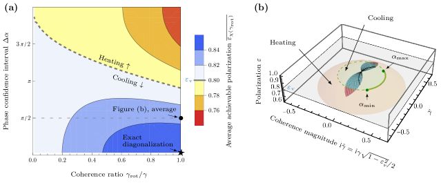
Figure S4: Achievable target polarizations for unknown coherence phase. (a) Average achievable polarization $\overline{\varepsilon_{\chi(\gamma_{\text{rot}})}}$ of the target qubit over ensemble of states, Eq. (S14), for $\gamma_{\text{rot}}/\gamma<1$ and various confidence intervals $\Delta\alpha=\alpha_{\max}-\alpha_{\min}$, with $\alpha_{\text{rot}}=\alpha-\pi/2$ and $\varepsilon_{\textsl{v}}=0.8$. Average cooling is found for all values $\gamma_{\text{rot}}/\gamma$ when $\Delta\alpha<0.9\pi$. (b) Geometric representation (full green line) of ensemble of states for $\gamma=0.5$ with a confidence interval of $\alpha_{\min}=-\pi/4$ and $\alpha_{\max}=\pi/4$. The shaded region of achievable cooling (blue) and heating (red) is found by applying the unitary rotation with parameters $\gamma_{\text{rot}}=\gamma$ and $\alpha_{\text{rot}}=-\pi/2+\alpha$ for every point in the confidence interval (see corresponding average in (a)). The thicker black line represents the achievable target polarization region for fixed phase $\alpha_{\text{rot}}=(\alpha_{\max}-\alpha_{\min})/2$.

It is worthwhile mentioning that the above discussions on the achievable target polarization with incomplete information about the amount of coherence is based on a random density operator that depends on a stochastic variable ($\gamma$ or $\alpha$) specified by a probability distribution ($P(\gamma)$ or $P(\alpha)$). While a deterministic density operator characterizes the properties of a statistical ensemble, such a random density operator can be regarded as characterizing the statistical properties of an ensemble of ensembles bre02 . This ensemble of ensembles contains more information about a quantum system than the averaged ensemble, especially concerning fluctuation properties. For instance, the probability distributions ($P(\gamma)$ or $P(\alpha)$) allow us to determine in which cases it is possible to guarantee enhanced cooling of the target qubit for each individual realizations of the experiment, and not only on average.

Appendix E Coefficient of performance and cooling power

We analyze in this section the thermodynamic performance of the generalized, coherent three-qubit heat-bath algorithmic cooling example of the main text. The coefficient of performance $\zeta$ is a central figure of merit for refrigerators that is defined as the ratio of heat extracted and work supplied during the compression step, while the cooling power $J$ characterizes the rate of heat extraction. For discrete cooling cycles, there are given by sol22

$$\zeta(n)=-\frac{Q(n)}{W(n)}\quad\text{ and }J={|}Q(n+1)-Q(n){|}.$$ (S15)

In the presence of coherence, the definition of heat has to be extended to take the change of coherence properly into account ber20 ; ssu23 ; rod19 ; ham22 . The goal is to capture the cooling advantage provided by the manipulation of quantum coherence.

The heat extracted from the target qubit is concretely given by $-Q=-\tr_{1}H_{1}(\rho_{1}^{(n+1)}-\rho_{1}^{(n)})$, whereas work is defined as the total energy change over the target and two reset qubits during the compression step, $W=\sum_{i}\tr_{i}H_{i}(\rho_{i}^{(n+1)}-\rho_{i}^{(n)})$, with $i=1,2,3$. We can express these average energy changes in terms of the eigenvalues $\omega_{i}$ of $H_{i}$ and $p_{i}$ of $\rho_{i}$, as well as in terms of the transition amplitudes between the eigenbases of these two operators, $c_{ika}^{(n)}=\innerproduct{k}{n,a}_{i}$, where we admit possible changes in the qubit state eigenbases, $\ket{n,a}_{i}$. We accordingly obtain for the extracted heat

$$-Q=-\tr_{1}\{H_{1}(\rho_{1}^{(n+1)}-\rho_{1}^{(n)})\}=-\sum_{ka}\omega_{ik}\big{[}(\Delta p_{1a}^{(n)})|c_{1ka}^{(n)}|^{2}+p^{(n+1)}_{1a}\Delta(|c_{1ka}^{(n)}|^{2})\big{]},$$ (S16)

where $\Delta$ represents the cycle finite-difference of the $n$-dependent number on which it acts, e.g. $\Delta(|c_{ika}^{(n)}|^{2})=|c_{ika}^{(n+1)}|^{2}-|c_{ika}^{(n)}|^{2}$. This expression accounts for the possible cycle-dependence of the qubit eigenbasis.

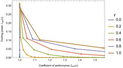
Figure S5: Cooling power $J_{\textrm{coh}}(n)$ against the coefficient of performance $\zeta_{\textrm{coh}}(n)$, Eq. (S19), for various values of the cycle number $n$ and different amounts of coherence $\gamma$. The coefficient of performance is enhanced in the presence of coherence $(\gamma>0)$ compared to the incoherent heat-bath algorithmic cooling prootocol $(\gamma=0)$. The initial target qubit polarization is $\varepsilon_{1}(0)=0$ and the two reset qubit polarizations are given by $\varepsilon_{2}=\varepsilon_{3}=0.5$.

We next define the coherent-energetic quantity ber20 ; ssu23

$$C_{i}=\sum_{ka}\omega_{ik}p_{ia}^{(n+1)}\Delta|c_{ika}^{(n)}|^{2},$$ (S17)

which is positive ($C_{i}>0$) whenever the qubit $i$ acquires coherence over a cycle. In order to include the contribution of quantum coherence to heat exchange, we introduce the ’coherent’ heat extracted from the target qubit ber20 ; ssu23

$$-\mathcal{Q}=-Q+C_{1}=-\sum_{ka}\omega_{ik}(\Delta p_{1a}^{(n)})|c_{1ka}^{(n)}|^{2}.$$ (S18)

Since the compression step is not modified, the work is left unchanged. We then obtain the coefficient of performance and cooling power of the generalized heat-bath algorithmic cooling protocol

$$\zeta_{\textrm{coh}}(n)=-\frac{\mathcal{Q}(n)}{W(n)}\quad\text{ and }\quad J_{\textrm{coh}}(n)=|\mathcal{Q}(n+1)-\mathcal{Q}(n)|.$$ (S19)

Figure S5 shows the power $J_{\textrm{coh}}(n)$ against the coefficient of performance $\zeta_{\textrm{coh}}(n)$ for various values of $n$ and different amounts of coherence $\gamma$. We note that the coefficient of performance is enhanced while the power is reduced in the presence of coherence $(\gamma>0)$ compared to the (standard) incoherent case $(\gamma=0)$. In particular, the coherent coefficient of performance, $\zeta_{\textrm{coh}}(n)$, can exceed the corresponding incoherent Carnot coefficient of performance, $\zeta_{\text{C}}(n)=T_{\text{c}}(n)/[T_{\text{h}}-T_{\text{c}}(n)]$, with the cold temperature, $T_{\text{c}}(n)=\ln[(1+\varepsilon_{1}(n))/(1-\varepsilon_{1}(n))]$ determined by the polarization of the target qubit, and the hot temperature $T_{\text{h}}$ set by the heat bath. This behavior is similar to that observed for a refrigerator in Ref. ham22 .

Appendix F Comparison with other resources

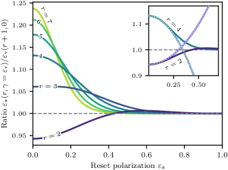
Figure S6: Quantum coherence versus one additional reset qubit. Ratio $\varepsilon_{\star}(r,\gamma=\varepsilon_{\textsl{v}})/\varepsilon_{\textsl{v}}(r+1,\gamma=0)$ of the maximum polarization attainable with $r$ reset qubits by adding coherence, $\gamma=\varepsilon_{\textsl{v}}$, and the maximum polarization obtainable by adding one more reset qubit without coherence ($\gamma=0$), as a function of the reset polarization $\varepsilon_{\textsl{a}}$, for various values of $r$. The coherent cooling scheme is better for moderate polarizations $\varepsilon_{\textsl{a}}$ for $r=2$ and for small polarizations $\varepsilon_{\textsl{a}}$ for $r\geq 3$. For small reset polarizations, the ratio depends quadratically on $\varepsilon_{\textsl{a}}$ (inset).

Another way to increase the target polarization in incoherent heat-bath algorithmic cooling is to augment the number of reset qubits rod16 . The asymptotic polarization grows exponentially with the number $r$ of reset qubits as $\varepsilon_{\infty}(r,\varepsilon_{\textsl{a}})=[(1+\varepsilon_{\textsl{a}})^{r}-(1-\varepsilon_{\textsl{a}})^{r}]/[(1+\varepsilon_{\textsl{a}})^{r}+(1-\varepsilon_{\textsl{a}})^{r}]$, when all the reset qubits have the same polarization $\varepsilon_{\textsl{a}}$ rod16 . It is hence instructive to compare the cooling improvement achieved by the two, coherent and incoherent, methods. To that end, we consider a cooling algorithm with $r$ reset qubits com3 and define the ratio $\varepsilon_{\star}(r,\gamma=\varepsilon_{\textsl{v}})/\varepsilon_{\textsl{v}}(r+1,\gamma=0)$ of the maximum polarization attainable by adding the largest amount of coherence, $\gamma=\varepsilon_{\textsl{v}}$, to the corresponding virtual qubit and the maximum polarization obtainable by adding one more reset qubit in the absence of coherence ($\gamma=0$). Figure S6 displays this ratio as a function of the reset polarization $\varepsilon_{\textsl{a}}$, for different values of $r$. We observe that, for two reset qubits ($r=2$), adding coherence leads to a larger polarization than adding one reset qubit for moderate reset polarizations ($0.45<\varepsilon_{\textsl{a}}<0.9$), while both schemes are equivalent for high reset polarizations ($0.9<\varepsilon_{\textsl{a}}$). On the other hand, for $r\geq 3$, coherence appears to be always beneficial for smaller reset polarization, with an enhancement of more than $10\%$ for $r\geq 4$.

References

- (1) M. A. Nielsen and I. L. Chuang, Quantum Computation and Information, (Cambridge University Press, Cambridge, 2002).
- (2) P. Zanardi, Virtual Quantum Subsystems, Phys. Rev. Lett. 87, 077901 (2001).
- (3) P. Zanardi, D. A. Lidar, and S. Lloyd, Quantum Tensor Product Structures are Observable Induced, Phys. Rev. Lett. 92, 060402 (2004).
- (4) D. A. Lidar and T. A. Brun, Quantum Error Correction (Cambridge University Press, Cambridge, 2013).
- (5) E. Knill, R. Laflamme, and L. Viola, Theory of Quantum Error Correction for General Noise, Phys. Rev. Lett. 84, 2525 (2000).
- (6) D. Kribs, R. Laflamme, and D. Poulin, Unified and Generalized Approach to Quantum Error Correction, Phys. Rev. Lett. 94, 180501 (2005).
- (7) E. Knill, On protected realization of quantum information. Phys. Rev. A 74, 042301 (2006).
- (8) L.-M. Duan and G.-C. Guo, Preserving Coherence in Quantum Computation by Pairing Quantum Bits, Phys. Rev. Lett. 79, 1953 (1997).
- (9) P. Zanardi and M. Rasetti, Noiseless Quantum Codes, Phys. Rev. Lett. 79, 3306 (1997).
- (10) D. A. Lidar, I. L. Chuang, and K. B. Whaley, Decoherence-Free Subspaces for Quantum Computation, Phys. Rev. Lett. 81, 2594 (1998).
- (11) P. Zanardi and S. Lloyd, Topological Protection and Quantum Noiseless Subsystems, Phys. Rev. Lett. 90, 067902 (2003).
- (12) M.-D. Choi and D. W. Kribs, Method to find quantum noiseless subsystems, Phys. Rev. Lett. 96, 050501 (2006).
- (13) R. Blume-Kohout, H. K. Ng, D. Poulin, and L. Viola, Characterizing the Structure of Preserved Information in Quantum Processes, Phys. Rev. Lett. 100, 030501 (2008).
- (14) W. Dür and H.-J. Briegel, Entanglement Purification for Quantum Computation, Phys. Rev. Lett. 90, 067901 (2003).
- (15) J.-M. Cai, W. Dür, M. Van den Nest, A. Miyake, and H. J. Briegel, Quantum Computation in Correlation Space and Extremal Entanglement, Phys. Rev. Lett. 103, 050503 (2009).
- (16) J. Cai, A. Miyake, W. Dür, and H. J. Briegel, Universal quantum computer from a quantum magnet, Phys. Rev. A 82, 052309 (2010).
- (17) M. Popp, F. Verstraete, M. A. Martín-Delgado, and J. I. Cirac, Localizable entanglement, Phys. Rev. A 71, 042306 (2005).
- (18) O. Kabernik, J. Pollack, and A. Singh, Quantum state reduction: Generalized bipartitions from algebras of observables, Phys. Rev. A 101, 032303 (2020).
- (19) S. M. Carroll and A. Singh, Quantum mereology: Factorizing Hilbert space into subsystems with quasiclassical dynamics, Phys. Rev. A 103, 022213 (2021).
- (20) N. Brunner, N. Linden, S. Popescu, and P. Skrzypczyk, Virtual qubits, virtual temperatures, and the foundations of thermodynamics, Phys. Rev. E 85, 051117 (2012).
- (21) D. Venturelli, R. Fazio, and V. Giovannetti, Minimal Self-Contained Quantum Refrigeration Machine Based on Four Quantum Dots, Phys. Rev. Lett. 110, 256801 (2013).
- (22) L. A. Correa, J. P. Palao, G. Adesso, and D. Alonso, Performance bound for quantum absorption refrigerators, Phys. Rev. E 87, 042131 (2013).
- (23) J. Bohr Brask and N. Brunner, Small quantum absorption refrigerator in the transient regime: Time scales, enhanced cooling, and entanglement, Phys. Rev. E 92, 062101 (2015).
- (24) M. T. Mitchison, M. P. Woods, J. Prior and M. Huber, Coherence-assisted single-shot cooling by quantum absorption refrigerators, New J. Phys. 17, 115013 (2015).
- (25) R. Silva, G. Manzano, P. Skrzypczyk, and N. Brunner, Performance of autonomous quantum thermal machines: Hilbert space dimension as a thermodynamical resource, Phys. Rev. E 94, 032120 (2016).
- (26) Z.-X. Man and Y.-J. Xia, Smallest quantum thermal machine: The effect of strong coupling and distributed thermal tasks, Phys. Rev. E 96, 012122 (2017).
- (27) P. Erker, M. T. Mitchison, R. Silva, M. P. Woods, N. Brunner, and M. Huber, Autonomous Quantum Clocks: Does Thermodynamics Limit Our Ability to Measure Time?, Phys. Rev. X 7, 031022 (2017).
- (28) J. Y. Du and F. L. Zhang, Nonequilibrium quantum absorption refrigerator, New J. Phys. 20, 063005 (2018).
- (29) M. T. Mitchison, Quantum thermal absorption machines: refrigerators, engines and clocks, Contemp. Phys. 60, 164 (2019).
- (30) A. Rignon-Bret, G. Guarnieri, J. Goold, and M. T. Mitchison, Thermodynamics of precision in quantum nanomachines, Phys. Rev. E 103, 012133 (2021).
- (31) H. J. Metcalf and P. van der Straten, Laser Cooling and Trapping, (Springer, berlin, 1999).
- (32) V. S. Letokhov, Laser Control of Atoms and Molecules, (Oxford University Press, Oxford, 2007).
- (33) P. V. E. McClintock, D. J. Meredit and J. K. Wigmore, Low-Temperature Physics, (Springer, Berlin, 1992).
- (34) C. Ens and S. Hunklinger, Low-Temperature Physics, (Springer, Berlin, 2005).
- (35) E. Desurvire, Classical and Quantum Information Theory, (Cambridge University Press, Cambridge, 2009).
- (36) J. D. Hidary, Quantum Computing: An Applied Approach, (Springer, Berlin, 2021).
- (37) W. Ketterle and D. E. Pritchard, Atom cooling by time-dependent potentials, Phys. Rev. A 46, 4051 (1992).
- (38) X. Wang, S. Vinjanampathy, F. W. Strauch, and K. Jacobs, Absolute dynamical limit to cooling weakly coupled quantum systems. Phys. Rev. Lett. 110, 157207 (2013).
- (39) L. A. Wu, D. Segal and P. Brumer, No-go theorem for ground state cooling given initial system-thermal bath factorization, Sci. Rep. 3, 1824 (2013).
- (40) F. Ticozzi and L. Viola, Quantum resources for purification and cooling: fundamental limits and opportunities, Sci. Rep. 4, 5192 (2014).
- (41) A. E. Allahverdyan, K. V. Hovhannisyan, D. Janzing, and G. Mahler, Thermodynamic limits of dynamic cooling, Phys. Rev. E 84, 041109 (2011).
- (42) D. Reeb and M. M. Wolf, An improved Landauer principle with finite-size corrections, New J. Phys. 16, 103011 (2014).
- (43) F. Clivaz, R. Silva, G. Haack, J. Bohr Brask, N. Brunner, and M. Huber, Unifying Paradigms of Quantum Refrigeration: A Universal and Attainable Bound on Cooling, Phys. Rev. Lett. 123, 170605 (2019).
- (44) F. Clivaz, R. Silva, G. Haack, J. Bohr Brask, N. Brunner, and M. Huber, Unifying paradigms of quantum refrigeration: Fundamental limits of cooling and associated work costs, Phys. Rev. E 100, 042130 (2019).
- (45) L. J. Schulman and U. V. Vazirani, Molecular scale heat engines and scalable quantum computation, Proc. 31st ACM Symp. on Theory of Computing, 322 (ACM Press, 1999).
- (46) P. O. Boykin, T. Mor, V. Roychowdhury, F. Vatan, and R. Vrijen, Algorithmic cooling and scalable NMR quantum computers. Proc. Natl Acad. Sci. USA 99, 3388 (2002).
- (47) D. K. Park, N. A. Rodriguez-Briones, G. Feng, R. R. Darabad, J. Baugh, and R. Laflamme, Heat Bath Algorithmic Cooling with Spins: Review and Prospects, Electron spin resonance (ESR) based quantum computing. Biological Magnetic Resonance. 31, 227 (2016).
- (48) J. M. Fernandez, S. Lloyd, T. Mor, and V. Roychowdhury, Algorithmic cooling of spins: a practicable method for increasing polarization, Int. J. Quantum Inf. 2, 461 (2004).
- (49) L. J. Schulman, T. Mor, and Y. Weinstein, Physical limits of heat-bath algorithmic cooling, Phys. Rev. Lett. 94, 120501 (2005).
- (50) L. J. Schulman, T. Mor, and Y. Weinstein, Physical limits of heat-bath algorithmic cooling, SIAM J. Comput. 36, 1729 (2007).
- (51) F. Rempp, M. Michel, and G. Mahler, Phys. Rev. A 76, 032325 (2007).
- (52) P. Kaye, Cooling algorithms based on the 3-bit majority, Quantum Inf. Process. 6, 295 (2007).
- (53) G. Brassard, Y. Elias, T. Mor, Y. Weinstein, Prospects and Limitations of Algorithmic Cooling, Eur. Phys. J. Plus 129, 258 (2014).
- (54) S. Raeisi and M. Mosca, Asymptotic bound for heat-bath algorithmic cooling, Phys. Rev. Lett. 114, 100404 (2015).
- (55) N. A. Rodriguez-Briones and R. Laflamme, Achievable polarization for heat-bath algorithmic cooling, Phys. Rev. Lett. 116, 170501 (2016).
- (56) S. Raeisi, M. Kieferov, and M. Mosca, Novel technique for robust optimal algorithmic cooling, Phys. Rev. Lett. 122, 220501 (2019).
- (57) R. Soldati, D. B. R. Dasari, J. Wrachtrup, and E. Lutz, Thermodynamics of a minimal algorithmic cooling refrigerator, Phys. Rev. Lett. 129, 030601 (2022).
- (58) A virtual quantum subsystem of a larger system is associated with a tensor factor of a subspace of such that , for some factor and a remainder space , see, for example, Ref. tic14 .
- (59) R. Kosloff and A. Levy, Quantum Heat Engines and Refrigerators: Continuous Devices, Annu. Rev. Phys. Chem. 65, 365 (2014).
- (60) I. Bengtsson and K. Zyckowski, The Geometry of Quantum States, (Cambridge University Press, Cambridge, 2006).
- (61) We emphasize that the final unitary rotation applies to the qubit system and not to the virtual qubit. This is experimentally advantageous since virtual qubits are often encoded in complex multipartite systems.
- (62) M. Le Bellac, F. Mortessagne and G.G. Batrouni, Equilibrium and Non-Equilibrium Statistical Thermodynamics, (Cambridge University Press, Cambridge, 2004).
- (63) This amounts to an inexact diagonalization of the virtual state, in contrast to the exact diagonalization that lead to the optimal bound (2).
- (64) See Supplemental Material.
- (65) The worst case overall is for the pair of values , where the state is heated to .
- (66) J. Baugh, O. Moussa, C. A. Ryan, A. Nayak, and R. Laflamme, Experimental implementation of heat-bath algorithmic cooling using solid-state nuclear magnetic resonance, Nature 438, 470 (2005).
- (67) C. A. Ryan, O. Moussa, J. Baugh, and R. Laflamme, Spin based heat engine: Demonstration of multiple rounds of algorithmic cooling, Phys. Rev. Lett. 100, 140501 (2008).
- (68) D. K. Park, G. Feng, R. Rahimi, S. Labruyere, T. Shibata, S. Nakazawa, K. Sato, T. Takui, R. Laflamme, and J. Baugh, Hyperfine spin qubits in irradiated malonic acid: heat-bath algorithmic cooling, Quantum Inf. Process. 14, 2435 (2015).
- (69) Y. Atia, Y. Elias, T. Mor, and Y. Weinstein, Algorithmic cooling in liquid-state nuclear magnetic resonance, Phys. Rev. A 93, 012325 (2016).
- (70) S. Zaiser, C. T. Cheung, S. Yang, D. B. R. Dasari, S. Raeisi and J. Wrachtrup, Cyclic cooling of quantum systems at the saturation limit, npj Quant. Info. 7, 92 (2021).
- (71) P. M. Harrington, E. J. Mueller, and K. W. Murch, Engineered dissipation for quantum information science, Nat. Rev. Phys. 4, 660 (2022).
- (72) J. Watrous, The Theory of Quantum Information, (Cambridge University Press, Cambridge, 2018).
- (73) J. A. Gyamfi, Fundamentals of quantum mechanics in Liouville space, Eur. J. Phys. 41, 063002 (2020).
- (74) R. Soldati, D. B. R. Dasari, J. Wrachtrup, and E. Lutz, Thermodynamics of a Minimal Algorithmic Cooling Refrigerator, Phys. Rev. Lett. 129, 030601 (2022).
- (75) H.-P. Breuer and F. Petruccione, The Theory of Open Quantum Systems, (Oxford University Press, Oxford, 2002).
- (76) B. de Lima Bernardo, Unravelling the role of coherence in the first law of quantum thermodynamics, Phys. Rev. E 102, 062152 (2020).
- (77) J. Chen, Y. Wang, G. Su, J. Chen, and S. Su, The general expressions of heat and work in two representations of quantum mechanics, Physica A 609, 128389 (2023).
- (78) F. L. S. Rodrigues, G. De Chiara, M. Paternostro, and G. T. Landi, Thermodynamics of Weakly Coherent Collisional Models, Phys. Rev. Lett. 123, 140601 (2019).
- (79) K. Hammam, H. Leitch, Y. Hassouni, and G. De Chiara, Exploiting coherence for quantum thermodynamic advantage, New J. Phys. 24, 113053 (2022).
- (80) N. A. Rodriguez-Briones and R. Laflamme, Achievable polarization for heat-bath algorithmic cooling, Phys. Rev. Lett. 116, 170501 (2016).
- (81) The virtual qubit of the incoherent heat-bath algorithmic cooling protocol with reset qubits of Ref. rod16 is given by the two states ( times ) and ( times ) of the multi reset qubit system.