Dust-Obscured Galaxies in the XMM-SERVS Fields: Selection, Multiwavelength Characterization, and Physical Nature

Abstract

Dust-obscured galaxies (DOGs) are enshrouded by dust, and many are believed to host accreting supermassive black holes (SMBHs), which makes them unique objects for probing the coevolution of galaxies and SMBHs. We select and characterize DOGs in the $13\,\deg^{2}$ XMM-Spitzer Extragalactic Representative Volume Survey (XMM-SERVS), leveraging the superb multiwavelength data from X-rays to radio. We select 3738 DOGs at $z\approx 1.6-2.1$ in XMM-SERVS, while maintaining good data quality without introducing significant bias. This represents the largest DOG sample with thorough multiwavelength source characterization. Spectral energy distribution (SED) modeling shows DOGs are a heterogeneous population consisting of both normal galaxies and active galactic nuclei (AGNs). Our DOGs are massive ($\log M_{\star}/M_{\sun}\approx 10.7-11.3$), 174 are detected in X-rays, and they are generally radio-quiet systems. X-ray detected DOGs are luminous and are moderately to heavily obscured in X-rays. Stacking analyses for the X-ray undetected DOGs show highly significant average detections. Critically, we compare DOGs with matched galaxy populations. DOGs have similar AGN fractions compared with typical galaxy populations. X-ray detected DOGs have higher $M_{\star}$ and higher X-ray obscuration, but they are not more star-forming than typical X-ray AGNs. The results potentially challenge the relevance of the merger-driven galaxy-SMBH coevolution framework for X-ray detected DOGs.

1 Introduction

Over the past couple of decades, astronomers have developed a coevolution framework between supermassive black holes (SMBHs) and galaxies (e.g., Sanders et al., 1988; Di Matteo et al., 2005; Hopkins et al., 2006). As cold gas accumulates, for example, major mergers can trigger strong star formation (SF) in host galaxies; gas reservoirs also fuel the accretion of central SMBHs, allowing them to be observed as AGNs. Contemporaneously, gas and dust can enshroud the nucleus and cause severe obscuration. AGN feedback also further impacts host galaxies, in which AGN outflows and radiation may suppress SF activity. Such a coevolution framework provides a possible explanation for how the central AGN impacts its host galaxy.

Since the commissioning of wide-field infrared (IR) observatories like the Spitzer Space Telescope and Wide-field Infrared Survey Explorer (WISE), studies of dusty galaxies have been greatly advanced as dust emission can be directly traced by IR observations. Dey et al. (2008) used Spitzer data to efficiently select a sample of dust-obscured galaxies (DOGs) at $z\approx 1.5-3$ with $f_{\mathrm{24\mu m}}>0.3\,\mathrm{mJy}$ and $(R-[24])_{\mathrm{Vega}}\geq 14$, where $[24]$ is the magnitude at $24\,\mathrm{\mu m}$. Toba & Nagao (2016) applied different selection criteria using WISE with $f_{\mathrm{22\mu m}}>3.8\,\mathrm{mJy}$ and $i-[22]\geq 7$ to select the so-called IR-bright DOGs, which are a subpopulation of hyperluminous IR galaxies (HyLIRGs; $L_{\mathrm{IR}}>10^{13}L_{\sun}$), where $[22]$ is the AB magnitude at $22\,\mathrm{\mu m}$. These galaxies constitute a substantial fraction of the IR luminosity density among ultraluminous IR galaxies ($L_{\mathrm{IR}}>10^{12}L_{\sun}$) (e.g., Toba et al., 2015, 2017). Eisenhardt et al. (2012) and Wu et al. (2012) applied the WISE “W1W2-dropout” technique to select an even more extreme subpopulation among HyLIRGs. These objects are similar to DOGs but have higher dust temperatures (up to hundreds of K versus $30-40\,\rm K$), and are therefore dubbed Hot DOGs (e.g., Tsai et al., 2015; Assef et al., 2016; Vito et al., 2018). For them, the bolometric luminosity ($L_{\mathrm{bol}}$) is dominated by IR emission, with the most extreme sources reaching to $L_{\mathrm{bol}}\gtrsim 10^{14}\,L_{\sun}$ (e.g., Tsai et al., 2015; Vito et al., 2018).

The strong IR emission from these types of dusty galaxies can be explained by intense SF activity, along with potential contributions from central AGNs that are buried beneath obscuring gas and dust (e.g., Fiore et al., 2008; Lanzuisi et al., 2009; Eisenhardt et al., 2012; Vito et al., 2018; Toba et al., 2020a). Phenomologically, based upon the spectral energy distribution (SED) shape in the mid-infrared (MIR), DOGs can be classified as “Power-Law” (PL) or “Bump” DOGs. PL DOGs exhibit a fairly monotonic MIR SED, while the Bump DOGs show a distinct SED “bump” at observed-frame $\approx 3-10\,\mathrm{\mu m}$, possibly due to stellar continuum peaking at rest-frame $\approx 1.6\,\mathrm{\mu m}$ (e.g., Dey et al., 2008; Melbourne et al., 2012; Toba et al., 2015). The fraction of PL DOGs generally increases with IR flux density, and their SED shape appears to be more AGN-like (e.g., Melbourne et al., 2012). Therefore, PL DOGs are generally thought to correspond to AGN-dominated sources, while Bump DOGs correspond to galaxies undergoing strong SF. Both observations and simulations suggest that DOGs evolve from Bump to PL phase (e.g., Dey & NDWFS/MIPS Collaboration, 2009; Bussmann et al., 2012; Yutani et al., 2022), indicating a possible link with the merger-driven galaxy-SMBH coevolution framework.

X-ray observations can provide further evidence of AGN activity due to the reduced absorption bias of X-rays and the large contrast between the X-ray emission of AGNs and stellar components (e.g., Brandt & Yang, 2022). The typical fraction of X-ray detected DOGs is $\approx 10-20\%$, depending on the X-ray depth of the fields (e.g., Fiore et al., 2008; Corral et al., 2016; Riguccini et al., 2019). It is found that X-ray detected DOGs generally have moderate-to-high $L_{\mathrm{X}}$ ($2-10\,\mathrm{keV}$ $L_{\mathrm{X}}\approx 10^{43.5}-10^{45}\,\mathrm{erg}\,\mathrm{s}^{-1}$) with a wide range of $N_{\mathrm{H}}$ from moderate to Compton-thick (CT) levels (e.g., Fiore et al., 2008; Lanzuisi et al., 2009; Stern et al., 2014; Corral et al., 2016; Riguccini et al., 2019; Toba et al., 2020b; Kayal & Singh, 2024). Studies have attempted to characterize and search for connections between AGN luminosity, obscuration, and host-galaxy properties for different types of dusty galaxies to understand how they are related to the merger-driven galaxy-SMBH coevolution framework. In particular, X-ray studies of the most extreme Hot DOGs show that they are significantly more obscured in X-rays and have comparable or slightly lower X-ray luminosity than optical type 1 quasars with similar $L_{\mathrm{bol}}$, which indicates that Hot DOGs are caught during extreme SMBH accretion and are likely in the late stage of major mergers (Vito et al., 2018). However, contrary results are found for X-ray-selected heavily obscured AGNs, which have less extreme optical-IR colors than DOGs. Systematic studies of the origins of their X-ray obscuration and its correlation with host-galaxy properties and morphologies indicate that they are more likely triggered by secular processes instead of mergers (Li et al., 2020). As for DOGs, theoretical studies suggest that they are in the end stage of major mergers where they are at the peak of SF and starting to transition to the AGN-dominated phase (e.g., Hopkins et al., 2006; Narayanan et al., 2010; Yutani et al., 2022); observational studies of the morphology and dust properties of DOGs give some evidence supporting the relevance of the merger-driven coevolution framework for DOGs (e.g., Bussmann et al., 2012), but the results are limited by low-resolution images and small sample sizes (Netzer, 2015). Recent results from the James Webb Space Telescope (JWST) on small samples of submillimeter galaxies (SMGs), which are dust-enshrouded like DOGs, show that most of them have non-disturbed disks, suggesting that they may grow via secular processes (e.g., Cheng et al., 2023; Gillman et al., 2023; Le Bail et al., 2024).

Although the widely used color-based criteria can efficiently select large samples of DOGs, source characterization is often poor due to, e.g., limited multiwavelength coverage, which hinders further detailed analysis to understand their properties. For instance, Dey et al. (2008) selected $\approx 2600$ DOGs in the $\approx 8.1\,\deg^{2}$ NOAO Deep Wide-Field Survey Boötes field, but they were only able to study the IR properties of 86 sources with available spectroscopic redshifts (spec-$z$s). Similarly, Toba & Nagao (2016) selected 5311 IR-bright DOGs using WISE across 14555$\,\deg^{2}$, but only 67 sources have reliable spec-$z$s. Studies also searched for DOGs in deep and medium-deep fields (e.g., the Cosmic Evolution Survey; COSMOS) where source characterization may be more secure. Riguccini et al. (2019) selected far-infrared (FIR) detected DOGs in COSMOS, but since its sky area is relatively small ($\approx 2.2\,\deg^{2}$), there were only 108 sources in the final sample.

In this work, we select DOGs in the XMM-Spitzer Extragalactic Representative Volume Survey (XMM-SERVS) fields (Chen et al., 2018; Ni et al., 2021) and investigate their nature by analyzing their multiwavelength properties. XMM-SERVS, with $13\deg^{2}$ of coverage, contains the prime parts of three Deep-Drilling Fields (DDFs) of the Legacy Survey of Space and Time (LSST): Wide Chandra Deep Field-South (W-CDF-S; $4.6\deg^{2}$), European Large Area Infrared Space Observatory Survey-S1 (ELAIS-S1; $3.2\deg^{2}$), and XMM-Newton Large-Scale Structure (XMM-LSS; $5.3\deg^{2}$). These fields provide a large search volume with superb, uniform multiwavelength coverage from X-rays to radio. Additionally, XMM-SERVS has excellent prospects for future development as it has been selected for further photometric and spectroscopic surveys, including LSST (e.g., Ivezić et al., 2019), Euclid (e.g., Euclid Collaboration et al., 2024), Large Millimeter Telescope (LMT) TolTEC (e.g., Wilson et al., 2020), Multi-Object Optical and Near-IR Spectrograph (MOONS; e.g., Cirasuolo et al., 2020), Subaru Prime Focus Spectrograph (PFS; e.g., Takada et al., 2014), and 4-meter Multi-Object Spectroscopic Telescope Wide-Area VISTA Extragalactic Survey (4MOST WAVES; e.g., Driver et al., 2019).

This work presents a multiwavelength study of a large sample of DOGs in the XMM-SERVS fields with an emphasis on their X-ray properties. We aim to explore the origin of their X-ray emission, and how the obscuration is related to the host-galaxy properties. Critically, we assess if DOGs fit into the merger-driven galaxy-SMBH coevolution framework by comparing their properties with a control sample of X-ray AGNs.

The structure of this paper is as follows. In Section 2, we present our sample selection. Section 3 presents our analyses and results on the multiwavelength properties of DOGs. We discuss the physical implications and test the relevance of the merger-driven galaxy-SMBH framework for DOGs in Section 4. Finally, we summarize our work in Section 5.

Throughout this paper, we adopt a flat $\Lambda$CDM cosmology with $H_{0}=70\,\rm km\,s^{-1}\,Mpc^{-1}$, $\Omega_{\Lambda}=0.70$, and $\Omega_{\mathrm{M}}=0.30$. Magnitudes are given in the AB system unless otherwise specified. We use the nonparametric $k$-sample Anderson-Darling (AD) test for hypothesis testing, and a significance level of $\alpha=0.001$ is adopted. The AD test is generally more effective than other similar nonparametric tests, such as the two-sample Kolmogorov-Smirnov (KS) test, because it provides more uniform sensitivity across the full ranges of the tested distributions (e.g., Stephens, 1974; Hou et al., 2009; Feigelson & Babu, 2012). We have verified that the statistical results using KS tests are not significantly different from those obtained with AD tests in this paper.

2 Data and Sample Selection

2.1 Initial Selection

Our DOGs are selected in the XMM-SERVS fields. As per Section 1, the XMM-SERVS fields are covered by superb multiwavelength surveys from X-rays to radio. These surveys include

1. X-ray: XMM-SERVS (Chen et al., 2018; Ni et al., 2021).

2. UV: the Galaxy Evolution Explorer (GALEX; Martin et al., 2005).

3. Optical: the Hyper Suprime-Cam (HSC) Subaru Strategic Program (Aihara et al., 2018), HSC imaging in the W-CDF-S (Ni et al., 2019), the VST Optical Imaging of the CDF-S and ELAIS-S1 (VOICE; Vaccari et al., 2016), the ESO-Spitzer Imaging extragalactic Survey (ESIS; Berta et al., 2006), the Dark Energy Survey (DES; Abbott et al., 2021), and the Canada-France-Hawaii Telescope Legacy Survey (CFHTLS; Hudelot et al., 2012).

4. Near-infrared (NIR): the VISTA Deep Extragalactic Observations (VIDEO; Jarvis et al., 2013) survey.

5. Mid-infrared (MIR) and far-infrared (FIR): the Spitzer DeepDrill survey (DeepDrill; Lacy et al., 2021), the Spitzer Wide-area Infrared Extragalactic survey (SWIRE; Lonsdale et al., 2003), and the Herschel Multi-tiered Extragalactic Survey (HerMES; Oliver et al., 2012).

6. Radio: the Australia Telescope Large Area Survey (ATLAS; e.g., Franzen et al., 2015), the VLA survey (e.g., Heywood et al., 2020), and the MeerKAT International GHz Tiered Extragalactic Exploration (MIGHTEE; Jarvis et al., 2013; Heywood et al., 2022) survey.

All of these surveys are utilized in our work. For detailed lists of covered surveys, see Table 1 of Zou et al. (2022) and Table 1 of Zhu et al. (2023).

Among the aforementioned surveys, the Spitzer $24\,\rm\mu m$ coverage reaches $0.1\,\mathrm{mJy}$ at $5\sigma$ depth (Lonsdale et al., 2004), which is sufficient to completely sample DOGs (defined as having $f_{\mathrm{24\mu m}}>0.3\,\mathrm{mJy}$). The X-ray survey made by XMM-Newton has a roughly uniform $50\,\rm ks$ exposure across the fields, reaching a flux limit of $\approx 10^{-15}-10^{-14}\,\mathrm{erg}\,\mathrm{cm}^{-2}\,\mathrm{s}^{-1}$ at $0.5-10\,\mathrm{keV}$. The survey is currently the largest medium-depth X-ray survey and has provided over 10200 AGNs. Additionally, sensitive radio surveys at $1.4\,\rm GHz$ ($5\sigma$ flux limit $\approx 28-85\,\rm\mu Jy$) allow us to perform systematic radio analyses of DOGs. Moreover, the $0.36-4.5\,\rm\mu m$ photometry has been refined via a forced-photometry technique to reduce source confusion and ensure consistency among different bands (Nyland et al., 2017, 2023; Zou et al., 2021a). The forced photometry utilizes deep fiducial images from the VIDEO survey. The spec-$z$s are taken from several spectroscopic surveys, and the photometric redshifts (photo-$z$s) are compiled from Ni et al. (2021) and Zou et al. (2021b) for W-CDF-S and ELAIS-S1, and from Chen et al. (2018) for XMM-LSS. The photo-$z$s are primarily calculated using the photo-$z$ code EAZY (Brammer et al., 2008), which estimates photo-$z$ by fitting the observed photometry with various galaxy (and optionally, AGN) templates. Although the photo-$z$s in XMM-SERVS generally have high quality with a catastrophic outlier fraction of a few percent, we will show in Section 2.2 that, for DOGs particularly, the photo-$z$ quality is not optimal and requires additional quality cuts to ensure reliable source characterization.

Utilizing the X-ray to FIR coverage, Zou et al. (2022) have measured the host-galaxy properties including stellar mass ($M_{\star}$) and star-formation rate (SFR) in XMM-SERVS via fitting the SED with CIGALE (Boquien et al., 2019; Yang et al., 2022), where the AGN emission has been properly considered. We will use the catalogs provided by Zou et al. (2022) as our parent sample. Note that CIGALE is not used as a photo-$z$ estimator.

We filter out stellar objects reported in Zou et al. (2022) and apply the same criteria as in Dey et al. (2008) to select our preliminary DOG sample, i.e., $f_{\mathrm{24\mu m}}>0.3\,\mathrm{mJy}$ and $f_{\mathrm{24\mu m}}/f_{R}\geq 982$, where $f_{\mathrm{24\mu m}}$ and $f_{R}$ are the observed-frame flux densities at $24\,\mu\rm m$ and in the $R$ band, respectively. The selection is done in three steps. First, we restrict our sample region to the intersection of the footprints cataloged by Zou et al. (2022), the $R$-band coverage, the $24\,\mathrm{\mu m}$ coverage, and the X-ray coverage. This results in $\approx 2.2$ million sources within a $\approx 20\%$ smaller area than XMM-SERVS: $3.5\deg^{2}$ in W-CDF-S, $2.7\deg^{2}$ in ELAIS-S1, and $4.1\deg^{2}$ in XMM-LSS. Second, we apply $f_{\mathrm{24\mu m}}>0.3\,\mathrm{mJy}$ in our sample region and select 31853 sources. After that, we convert the $R$-band magnitude measured through different $R$ filters in XMM-SERVS (see Table 1 in Zou et al., 2022) to the same $R$ filter used in Dey et al. (2008) using their best-fit SED for consistency. The correction is generally small. For sources with non-positive $R$-band flux measured in forced photometry, we use the $R$-band flux estimated from their best-fit SED. Finally, we apply $f_{\mathrm{24\mu m}}/f_{R}\geq 982$ and obtain 3738 sources in XMM-SERVS. The sky density of our selected DOGs ($363\,\deg^{-2}$) is similar to that in Dey et al. (2008) ($\approx 321\,\deg^{-2}$). There are 174 DOGs detected in X-rays. The median net source counts at $0.5-10\,\mathrm{keV}$ of the X-ray detected DOGs are 128 for all XMM-Newton EPIC cameras (PN, MOS1, and MOS2) combined, and the corresponding $25-75\%$ quantile range is $87-200$. We refer to these 3738 DOGs as our “full sample”.

It is worth noting that our forced photometry utilizes the reddest VIDEO band in which the source is detected as the fiducial band. We further examine the VIDEO $K_{S}$ band magnitude distributions for all sources with $f_{24\,\rm\mu m}>0.3\,\mathrm{mJy}$. These sources (median $K_{S}=19.4$) are generally much brighter than the $K_{S}$ magnitude limit ($K_{S}=24$) in our fields, and only $\approx 0.6\%$ are fainter than the $K_{S}$ magnitude limit. The results indicate that we do not miss a significant fraction of sources with $f_{24\,\rm\mu m}>0.3\,\mathrm{mJy}$ in our fiducial images, and our forced photometry allows us to sample almost all the DOGs in our search volume.

We show the $f_{\mathrm{24\mu m}}/f_{R}$ versus $f_{\mathrm{24\mu m}}$ distribution for the 3738 selected DOGs and all $24\,\rm\mu m$-detected galaxies in XMM-SERVS in Figure 1. By construction, DOGs have higher $f_{\mathrm{24\mu m}}$ and are redder than typical galaxies. Among our DOGs, only $0.9\%$ (31) have available spec-$z$s. Most of these sources lack detailed classification of galaxy/AGN type or publicly available spectra. We are able to identify one object as a type 1 AGN and one as a type 2 AGN, both observed by the Sloan Digital Sky Survey (Abdurro’uf et al., 2022). The spec-$z$ fraction is much smaller than that generally for XMM-SERVS ($\approx 4\%$), due to the faintness in optical bands imposed by our selection criteria. Thus, the majority of our sources only have photo-$z$s available. For illustration, we show a typical collection of four DOGs in Figure 2. In the next subsection, we will further assess the reliability of the photo-$z$s.

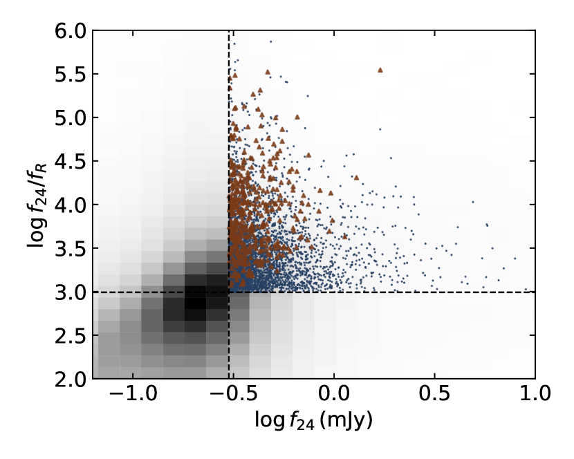
Figure 1: The $f_{\mathrm{24\mu m}}/f_{R}$ versus $f_{\mathrm{24\mu m}}$ distribution. The dashed lines represent our color-selection thresholds, and sources in the upper-right region are selected as DOGs. The blue points represent DOGs with positive measured $R$-band flux. The brown up-triangles represent DOGs with non-positive $R$-band flux measured via forced photometry, whose $R$-band flux is estimated from the best-fit SED. The grayscale cells are the 2-D histogram for all $24\,\rm\mu m$-detected galaxies in XMM-SERVS, with darker cells representing more galaxies.

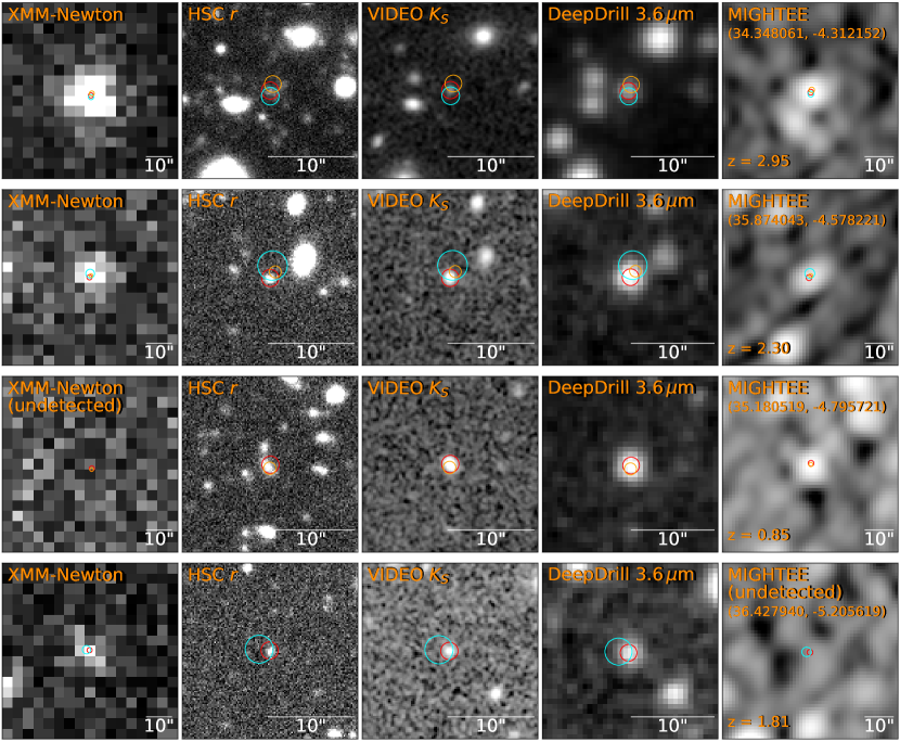
Figure 2: Illustrations of four DOGs in our full sample. For each source, we show the XMM-Newton 0.5–10 $\mathrm{keV}$ (first column; $60\arcsec\times 60\arcsec$), HSC $r$-band (second column; $20\arcsec\times 20\arcsec$), VIDEO $K_{S}$-band (third column; $20\arcsec\times 20\arcsec$), DeepDrill IRAC $3.6\,\mathrm{\mu m}$ (fourth column; $20\arcsec\times 20\arcsec$), and MIGHTEE $1.4\,\rm GHz$ (last column; $60\arcsec\times 60\arcsec$) images. The first two sources are detected in all five bands. The third source is not detected in X-rays, and the fourth source is not detected in radio. The VIDEO position and the redshift are shown in the last column for each source. X-ray positions are marked as cyan circles with a 68% error radius (Chen et al., 2018); VIDEO positions are marked as red circles with a $1\arcsec$ radius; and MIGHTEE positions are marked as orange circles with a 68% error radius (Zhu et al., 2023).

2.2 Additional Criterion for Reliable Redshifts

Although the photo-$z$s in Chen et al. (2018) and Zou et al. (2021b) are generally reliable, they are expected to be less reliable for our DOGs. This is mainly because DOGs are extreme sources whose SEDs may be significantly faint in the optical bands and lack strong spectral features (e.g., Pérez-González et al., 2005; Polletta et al., 2006; Dey et al., 2008), which makes it more difficult for photo-$z$ determination using SED fitting. Among the 31 DOGs with spec-$z$s, the outlier fraction ($f_{\mathrm{outlier}}$) for their photo-$z$s is $14/31=45\%$.

To minimize the impact of the above problem and reduce $f_{\mathrm{outlier}}$, we further select DOGs with more reliable photo-$z$s by employing the empirical photo-$z$ quality indicator, $Q_{z}$, defined in Equation 8 of Brammer et al. (2008). It combines several pieces of information when deriving photo-$z$s: the best-fit statistic, the number of photometric bands used, and the total integrated probability of photo-$z$ within $\pm 0.2$ of the best-fit photo-$z$. Small $Q_{z}$ indicates high reliability. A general threshold for reliable photo-$z$ is $Q_{z}<1$. However, this threshold may not be suitable for DOGs as they tend to be faint in the optical bands such that those bands do not necessarily provide useful constraints on the SED shape. Thus, we slightly modify the definition of $Q_{z}$: in Equation 8 of Brammer et al. (2008), instead of using the total number of bands, we only consider the number of “good” bands defined as having signal-to-noise ratio (SNR) greater than $3$. This new photo-$z$ quality indicator ($Q_{z}^{\mathrm{good}}$) is more indicative of the quality of photometric measurements for sources with extreme colors similar to DOGs. We consider a threshold of $Q_{z}^{\mathrm{good}}<1$ for high-quality photo-$z$s, which is more stringent than the nominal threshold of $Q_{z}<1$. Among our DOGs with $Q_{z}^{\mathrm{good}}<1$, the $f_{\mathrm{outlier}}$ for sources with spec-$z$ is reduced to $1/10=10\%$, indicating our $Q_{z}^{\mathrm{good}}<1$ cut can greatly improve the photo-$z$ quality for DOGs. The comparison between photo-$z$s and spec-$z$s for DOGs with spec-$z$ is shown in Figure 3.

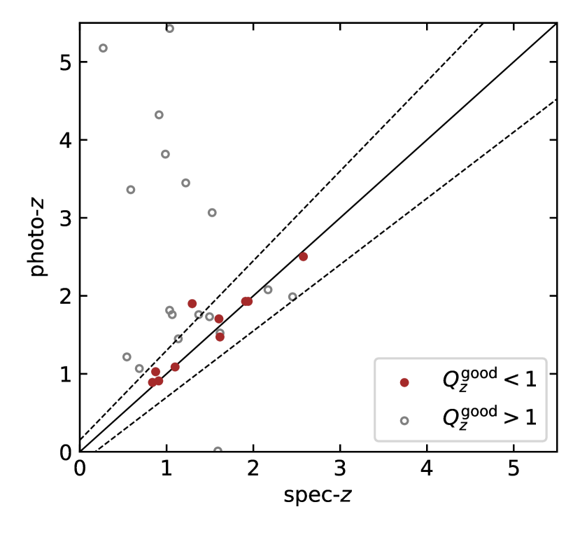
Figure 3: Comparison between the photo-$z$s and spec-$z$s for sources with spec-$z$ measurements. The brown solid circles represent sources with $Q_{z}^{\mathrm{good}}<1$. The grey empty circles are sources with $Q_{z}^{\mathrm{good}}>1$. The $Q_{z}^{\mathrm{good}}<1$ cut significantly reduces the outlier fraction. The solid line indicates the $z_{\mathrm{phot}}=z_{\mathrm{spec}}$ relation. The dashed lines represent the $|z_{\mathrm{phot}}-z_{\mathrm{spec}}|/(1+z_{\mathrm{spec}})>0.15$ relation.

In Figure 4, we plot the fraction of sources with high-quality photo-$z$s ($Q_{z}^{\mathrm{good}}<1$) as a function of $R$-band magnitude. The highest fraction of sources with $Q_{z}^{\mathrm{good}}<1$ is $\approx 55\%$ at $R\approx 24-25$. Toward the faint end, the fraction of sources with high-quality photo-$z$s decreases mainly due to the degradation of the photometric measurements. Toward the bright end, there is a decrease in the fraction. This arises from the increased fraction of sources hosting AGNs, and it has been found that larger fractional AGN contribution to the total flux will result in higher $Q_{z}$ values (e.g., Zou et al., 2023).

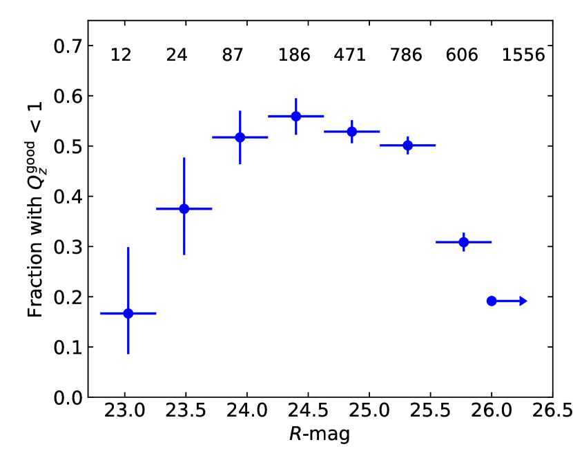
Figure 4: Fraction of sources in our full sample with $Q_{z}^{\mathrm{good}}<1$ as a function of $R$-mag. Each magnitude bin has a width of 0.45 mag except for the last one showing all sources with $R\text{-mag}>26$. The number above each bin shows the number of sources in the bin. The $y$-axis error bar represents the $1\sigma$ binomial confidence interval.

Out of our full sample of 3738 DOGs, we refer to the 1309 sources with spec-$z$s or $Q_{z}^{\mathrm{good}}<1$ to be our “core sample”, among which 88 are detected in X-rays. The median net source counts at $0.5-10\,\mathrm{keV}$ of the X-ray detected DOGs are 126, and the corresponding $25-75\%$ quantile range is $88-200$. We also test that at the bright end of Figure 4 ($R<24.5$), the fraction of X-ray detected DOGs in the core sample (19.4%) is similar to that in the full sample (20.3%), to some extent indicating that the $Q_{z}^{\mathrm{good}}$ cut does not preferentially exclude X-ray detected DOGs. Throughout the paper, we mainly report results for the core sample for a clear narrative flow, and we will show that the results for both samples are similar. A catalog containing all our selected DOGs is given in Table 1. We also summarize the subsamples used in this work in Table 2 for readability.

Table 1: Selected DOGs in XMM-SERVS.

Field	RA	Dec	Tractor ID	$z$	$z_{\mathrm{phot}}^{\mathrm{low}}$	$z_{\mathrm{phot}}^{\mathrm{up}}$	$z$-type	$Q_{z}^{\mathrm{good}}$	Core sample	XID	X-ray AGN	Reliable SED AGN	SED AGN candidate	Radio AGN via $q_{\mathrm{IR}}$	Radio AGN in Zhu et al. (2023)	$f_{\mathrm{24\mu\rm m}}$	Err{$f_{\mathrm{24\mu\rm m}}$}	$f_{\mathrm{24\mu\rm m}}/f_{R}$	$\log M_{\star}$	Err{$\log M_{\star}$}	$\log\rm SFR$	Err{$\log\rm SFR$}	$\log\mathrm{SFR_{norm}}$	Err{$\log\mathrm{SFR_{norm}}$}	$\log L_{\mathrm{bol}}$	$\log L_{\mathrm{1.4\,GHz}}$	Err{$\log L_{\mathrm{1.4\,GHz}}$}	$\alpha_{r}$	$\log L_{\mathrm{IR}}$	$\log L_{\mathrm{6\mu m,AGN}}$	Err{$\log L_{\mathrm{6\mu m,AGN}}$}	$f_{\mathrm{6\mu\rm m,AGN}}$	Err{$f_{\mathrm{6\mu\rm m,AGN}}$}	$\log L_{\mathrm{X,obs}}$	Err{$\log L_{\mathrm{X,obs}}$}	$\mathrm{HR}^{\mathrm{med}}$	$\mathrm{HR}^{\mathrm{low}}$	$\mathrm{HR}^{\mathrm{up}}$	$\log N_{\mathrm{H}}^{\mathrm{med}}$	$\log N_{\mathrm{H}}^{\mathrm{low}}$	$\log N_{\mathrm{H}}^{\mathrm{up}}$	lower-luminosity Hot DOG
	[deg]	[deg]														[mJy]	[mJy]		[$M_{\sun}$]	[$M_{\sun}$]	[$M_{\sun}$/yr]	[$M_{\sun}$/yr]			[$L_{\sun}$]	[W/Hz]	[W/Hz]		[W]	[$\mathrm{erg}\,\mathrm{s}^{-1}$]	[$\mathrm{erg}\,\mathrm{s}^{-1}$]			[$\mathrm{erg}\,\mathrm{s}^{-1}$]	[$\mathrm{erg}\,\mathrm{s}^{-1}$]				[$\mathrm{cm}^{-2}$]	[$\mathrm{cm}^{-2}$]	[$\mathrm{cm}^{-2}$]
(1)	(2)	(3)	(4)	(5)	(6)	(7)	(8)	(9)	(10)	(11)	(12)	(13)	(14)	(15)	(16)	(17)	(18)	(19)	(20)	(21)	(22)	(23)	(24)	(25)	(26)	(27)	(28)	(29)	(30)	(31)	(32)	(33)	(34)	(35)	(36)	(37)	(38)	(39)	(40)	(42)	(42)	(43)
W-CDF-S	51.912735	–28.035887	467148	3.32	2.37	3.43	photo-$z$	3.3652	0	WCDFS0256	1	1	1	1		0.535	0.019	2748	11.67	0.04	2.36	0.20	0.50	0.20	13.13	25.670	0.024	–99	39.60		0.03	0.87	0.06	44.45	0.08	–0.362	–0.511	–0.215	22.92	22.40	23.24	0
W-CDF-S	52.992867	–27.844992	505262	1.90	1.77	2.21	photo-$z$	0.3293	1	WCDFS2040	1	0	1	–1		0.882	0.017	1679	11.22	0.11	1.98	0.27	0.15	0.27	12.75	–99	–99	–99	39.24		0.13	0.76	0.09	44.29	0.10	–0.299	–0.460	–0.145	22.60	22.16	22.92	0
W-CDF-S	51.996666	–28.574844	328555	1.55	1.52	2.11	photo-$z$	1.1147	0	WCDFS0116	1	1	1	–1		1.328	0.017	4799	11.34	0.21	2.30	0.19	0.63	0.19	12.70	–99	–99	–99	39.16		0.16	0.86	0.06	43.81	0.10	–0.038	–0.378	0.256	22.92	22.28	23.28	0
W-CDF-S	52.026657	–28.955915	262032	1.65	1.50	1.68	photo-$z$	1.2292	0	WCDFS0149	1	1	1	–1		0.797	0.015	1289	11.25	0.05	1.99	0.11	0.26	0.11	12.63	–99	–99	–99	39.08		0.07	0.81	0.04	44.31	0.15	–0.209	–0.568	0.111	22.68	21.56	23.16	0
W-CDF-S	51.869560	–28.623209	456099	3.19	2.56	3.35	photo-$z$	4.8053	0	WCDFS0063	1	0	1	–1		0.325	0.020	1550	10.89	0.12	2.23	0.18	0.00	0.18	12.78	–99	–99	–99	39.18		0.06	0.84	0.08	45.16	0.11	–0.130	–0.274	–0.008	23.36	23.12	23.56	0

.

Note. — We only show five representative rows of our selected DOGs here. The full table is available as supplementary material. Column (1): field name. Columns (2) and (3): J2000 RA and Dec. Column (4): Tractor ID in Zou et al. (2022). Column (5): redshift. Columns (6) and (7): the 68% lower and upper limits of photo-$z$. Sources with spec-$z$ are assigned –1. Column (8): redshift type. Column (9): new photo-$z$ quality indicator defined in Section 2.2. Column (10): flag for our core sample defined in Section 2.2. Column (11): X-ray source ID in Chen et al. (2018) and Ni et al. (2021). Entries for sources not detected in X-rays are assigned –1. Column (12): flag for X-ray AGNs in Zou et al. (2020). Sources not detected in X-rays are assigned –1. Columns (13) and (14): flags for reliable SED AGNs, and SED AGN candidates in Zou et al. (2022). Column (15): flag for radio AGNs selected via $q_{\mathrm{IR}}$ in Zhang et al. (submitted). Sources not detected in radio are assigned –1. Column (16): flag for radio AGNs selected via $q_{24}$, morphology, or spectral index in Zhu et al. (2023). Sources not detected in radio are assigned –1. Columns (17) and (18): flux density at observed-frame $24\,\mu\rm m$ and its $1\sigma$ uncertainty. Column (19): $24\,\mu\rm m$-to-$R$ flux ratio. For the sources with non-positive $f_{R}$ via forced photometry, the $f_{R}$ is estimated from the best-SED, and the flux ratio is multiplied by –1. Columns (20) – (23): logarithms of best-fit $M_{\star}$ and SFR and their associated uncertainties in Zou et al. (2022). Columns (24) and (25): logarithms of $\mathrm{SFR_{norm}}$ and its $1\sigma$ uncertainty. The uncertainty only considers the contribution from SFR (see Section 2.3). Column (26): logarithms of bolometric luminosity. Columns (27) and (28): logarithms of rest-frame 1.4 GHz monochromatic luminosity and its $1\sigma$ uncertainty. Column (29): radio spectral slope calculated from measurements at 1.4 GHz and higher/lower frequencies. For W-CDF-S and ELAIS-S1, ATLAS 2.3 GHz is preferred over RACS. For XMM-LSS, LOFAR is preferred over RACS. Sources without multi-frequency measurements are assigned –99. Column (30): logarithms of total luminosity over rest-frame 8–1000 $\mu$m. Sources not detected in radio are assigned –99. Columns (31) and (32): logarithms of rest-frame $6\,\mu\rm m$ luminosity contributed by the AGN component and its $1\sigma$ uncertainty. Sources with best-fit normal-galaxy models are assigned –99. Columns (33) and (34): fractional AGN flux contribution at rest-frame $6\,\mu\rm m$ and its $1\sigma$ uncertainty. Sources with best-fit normal-galaxy models are assigned –99. Columns (35) and (36): logarithm of the observed X-ray luminosity at rest-frame 2–10 $\mathrm{keV}$ and its associated uncertainty. Columns (37)–(39) the median, 68% lower and upper limits of hardness ratio. Sources not detected in X-rays are assigned –99. Columns (40)–(42): the median, 68% lower and upper limits of the intrinsic column density calculated via hardness ratio. Sources not detected in X-rays are assigned –99. Column (43): flag for lower-luminosity Hot DOG candidates selected in Appendix B

Table 2: Summary of the major subsamples of our DOGs.

Subsample	Number in Full sample	Number in Core sample	Definition	First defined in Section
Total	3738	1309	$f_{\mathrm{24\mu m}}>0.3\,\mathrm{mJy}$ and $f_{\mathrm{24\mu m}}/f_{R}\geq 982$ in our sample region	2.1, 2.2
			Core sample has $Q_{z}^{\mathrm{good}}<1$
X-ray detected	174	88	Detected in X-rays	2.1
X-ray AGN	174	88	Identified as an X-ray AGN	2.4
			in Chen et al. (2018) or Ni et al. (2021)
X-ray undetected	3564	1221	Not detected in X-rays	2.3
Radio detected	745 (54)	317 (27)	Detected in radio	3.5
Radio AGN	172 (26)	73 (15)	Identified as a radio AGN
			in Zhu et al. (2023) or Zhang et al. (submitted)
SED AGN candidate	1887 (174)	523 (88)	Identified as a SED AGN candidate in Zou et al. (2022)	2.3
Reliable SED AGN	412 (79)	104 (37)	Identified as a reliable SED AGN in Zou et al. (2022)
Normal galaxy	1851 (0)	786 (0)	Not identified as a SED AGN candidate in Zou et al. (2022)
“Safe”	2808 (81)	874 (42)	$M_{\star}$ lower than the maximum $M_{\star}$ for reliable classification	3.1
			of star-forming galaxies in Equation 3, defined as
			the regions of the $z-M_{\star}$ plane where the fraction
			of quiescent galaxies less than 0.5 (Cristello et al., 2024)
Lower-luminosity Hot DOG	62 (1)	7 (0)	(1) $\rm W1-W4>9.7$ and $\rm W2-W4>8.2$ or	Appendix B
			(2) $\rm W1-W3>6.8$ and $\rm W2-W3>5.3$

Note. — The number of X-ray detected sources in the subsamples is shown in parentheses.

2.3 SED Fitting

In this subsection, we briefly explain the SED fitting and the SED-based classification in Zou et al. (2022). We will present our detailed analyses of the host-galaxy properties of our DOGs in Section 3.1. Interested readers can refer to Zou et al. (2022) for more details on the SED fitting in XMM-SERVS.

Zou et al. (2022) performed SED-fitting to classify non-stellar sources into AGN candidates and normal galaxies based upon calibrated Bayesian information criterion (BIC) and best-fit $\chi^{2}$ values; see their Section 3.2. They also classified a subset of AGN candidates as “reliable SED AGNs” based upon further calibrations against the ultradeep Chandra Deep Field-South with $7\,\rm Ms$ Chandra observations (CDF-S; Luo et al., 2017). The reliable SED AGNs are expected to reach a $\gtrsim 75\%$ purity, and the classification has been tested to be robust (see Section 3.2.4 of Zou et al., 2022). For each source, Zou et al. (2022) provided the best-fit SED model for the statistically preferred category. They also included normal-galaxy fitting results for all sources in the catalog. The SEDs are generally of high quality as the median number of photometric bands with $\mathrm{SNR}>5$ is 9, and $\approx 85\%$ of the sources have at least 7 photometric bands with $\mathrm{SNR}>5$ ranging from the UV to FIR.

Tables 3 and 4 summarize the CIGALE parameter settings for normal galaxies and AGN candidates in Zou et al. (2022). We have verified that the SED-fitting parameter settings are suitable even for extreme sources like DOGs via several tests. First, we have confirmed that the best-fit $E(B-V)$ values for our sources are well below the maximum allowed value of $E(B-V)=1.5$ in the settings, indicating that the reddening is acceptably modeled. Second, we test a more complex dust-emission module adopted from Draine et al. (2014) (dl2014), following the settings in Yang et al. (2023). In this test, the mass fraction of polycyclic aromatic hydrocarbons (PAHs) compared to total dust ($q_{\mathrm{PAH}}$) is allowed to be 0.47, 2.5, and 7.32, the minimum radiation field ($U_{\mathrm{min}}$) is allowed to vary from 0.1 to 50, the power-law slope ($\alpha$) is set to 2.0, and the fraction of the photodissociation region (PDR) is allowed to vary from 0.01 to 0.9. We find that the median differences for both $M_{\star}$ and SFR are only $\approx 0.1-0.2\,\rm dex$, and the normalized median absolute deviations ($\sigma_{\mathrm{NMAD}}$) are $\approx 0.2-0.3$, indicating general consistency between the two settings. Third, although there is no consensus on the exact star-formation history (SFH) for DOGs, Zou et al. (2022) applied a delayed SFH, which has proven to be generally reliable even for AGN-host and/or bursty galaxies (e.g., Carnall et al., 2019; Lower et al., 2020). We further test a truncated delayed SFH (sfhdelayedbq) and a periodic SFH (sfhperiodic) following the settings in Cristello et al. (submitted) and Suleiman et al. (2022), which are dedicated to the SED analyses for DOGs. For the sfhdelayedbq module, we allow the $e$-folding time and the stellar age to vary in the ranges $0.5-5\,\rm Gyr$ and $1-10\,\rm Gyr$, the burst/quench age ($t_{\mathrm{trun}}$) is allowed in the range $10-800\,\rm Myr$, the factor for instantaneous change of SFR at $t_{\mathrm{trun}}$ is allowed in the range $0.1-50$, and the other parameters are set to their default values. For the sfhperiodic module, the types of individual SF episodes are allowed as “exponential” or “delayed”, the period between each burst is allowed at 50 and 90$\,\rm Myr$, and the stellar age and the multiplicative factor for SFR are allowed in the ranges $0.1-10\,\rm Gyr$ and $1-4000$. The other parameters are set to their default values. For both types of SFHs, we do not find significant systematic differences in $M_{\star}$ or SFR (median differences are $\lesssim 0.2\,\rm dex$ and $\sigma_{\mathrm{NMAD}}\approx 0.2-0.3$).

To test further the reliability of our SFH, we fit the UV-to-NIR photometry of our normal-galaxy DOGs using the Prospector-$\alpha$ model within Prospector (Leja et al., 2017; Johnson et al., 2021). This model is flexible and incorporates a six-component nonparametric SFH, which mitigates any systematic biases caused by the choice of a parametric SFH. We exclude AGN candidates because Prospector is not optimized for AGN-dominated sources. We find that the median difference for the $M_{\star}$ is $\approx 0.3\,\rm dex$, and the median difference for SFR is $\approx 0.3\,\rm dex$. Furthermore, we verify that the best-fit SFHs generally do not exhibit recent starbursts (the median ratio of the SFR over the last $0-100\,\rm Myr$ compared to that over the last $100-300\,\rm Myr$ is only $\approx 2.3$), indicating our delayed SFH should be suitable to model the SF for DOGs. It is worth noting that there are generally systematic “factor-of-two” uncertainties among different SED-fitting results (e.g., Leja et al., 2019). This issue is inherent in SED-fitting methodologies, and solving it would require a more flexible SFH (e.g., a nonparametric SFH) at the cost of significantly higher computational requirements, which is beyond the scope of this work. Therefore, one should keep in mind possible systematic uncertainties depending on the adopted modules/parameter settings throughout this paper.

Table 3: CIGALE parameter settings for normal galaxies.

Module	Parameter	Name in the CIGALE configuration file	Possible values
Delayed SFH	Stellar $e$-folding time	tau_main	0.1, 0.2, 0.3, 0.4, 0.5, 0.6, 0.7, 0.8, 0.9,
			1, 2, 3, 4, 5, 6, 7, 8, 9, 10 Gyr
	Stellar age	age_main	0.1, 0.2, 0.3, 0.4, 0.5, 0.6, 0.7, 0.8, 0.9,
			1, 2, 3, 4, 5, 6, 7, 8, 9, 10 Gyr
Simple stellar population Bruzual & Charlot (2003)	Initial mass function	imf	Chabrier (2003)
	Metallicity	metallicity	0.0001, 0.0004, 0.004, 0.008, 0.02, 0.05
Nebular	–	–	–
Dust attenuation Calzetti et al. (2000)	$E(B-V)_{\mathrm{line}}$	E_BV_lines	0, 0.05, 0.1, 0.15, 0.2, 0.25, 0.3, 0.4
			0.5, 0.6, 0.7, 0.8, 0.9, 1, 1.2, 1.5
	$E(B-V)_{\mathrm{line}}/E(B-V)_{\mathrm{continuum}}$	E_BV_factor	1
Dust emission Dale et al. (2014)	Alpha slope	alpha	1.0, 1.25, 1.5, 1.75, 2.0, 2.25, 2.5, 2.75, 3.0
X-ray	–	–	–

Note. — Unlisted parameters are set to the default values. These are applied to all the sources.

Table 4: CIGALE parameter settings for AGN candidates.

Module	Parameter	Name in the CIGALE configuration file	Possible values
Delayed SFH	Stellar $e$-folding time	tau_main	0.1, 0.3, 0.5, 0.8, 1, 3, 5, 8, 10 Gyr
	Stellar age	age_main	0.1, 0.3, 0.5, 0.8, 1, 3, 5, 8, 10 Gyr
Simple stellar population Bruzual & Charlot (2003)	Initial mass function	imf	Chabrier (2003)
	Metallicity	metallicity	0.02
Nebular	–	–	–
Dust attenuation Calzetti et al. (2000)	$E(B-V)_{\mathrm{line}}$	E_BV_lines	0, 0.05, 0.1, 0.15, 0.2, 0.25, 0.3, 0.4
			0.5, 0.6, 0.7, 0.8, 0.9, 1, 1.2, 1.5
	$E(B-V)_{\mathrm{line}}/E(B-V)_{\mathrm{continuum}}$	E_BV_factor	1
Dust emission Dale et al. (2014)	Alpha slope	alpha	1.0, 1.25, 1.5, 1.75, 2.0, 2.25, 2.5, 2.75, 3.0
X-ray	AGN photon index	gam	1.8
	AGN $\alpha_{\mathrm{OX}}$	alpha_ox	-1.9, -1.8, -1.7, -1.6, -1.5,
			-1.4, -1.3, -1.2, -1.1
	Maximum deviation of $\alpha_{\mathrm{OX}}$ from the $\alpha_{\mathrm{OX}}-L_{\nu,2500}$ relation	max_dev_alpha_ox	0.2
	AGN X-ray angle coefficients	angle_coef	(0.5, 0)
AGN Stalevski et al. (2012, 2016)	Viewing angle	i	$0^{\circ}$, $10^{\circ}$, $30^{\circ}$, $50^{\circ}$, $70^{\circ}$, $90^{\circ}$
	Disk spectrum	disk_type	Schartmann et al. (2005)
	Modification of the optical power-law index	delta	–0.27
	AGN fraction	fracAGN	0, 0.05, 0.1, 0.2, 0.3, 0.4
			0.5, 0.6, 0.7, 0.8, 0.9, 0.99
	$E(B-V)$ of the polar extinction	EBV	0, 0.05, 0.1, 0.2, 0.3, 0.4, 0.5

Note. — Unlisted parameters are set to the default values. These are only applied to AGN candidates.

Since CIGALE requires absorption-corrected X-ray flux, Zou et al. (2022) applied a Bayesian approach to estimate the intrinsic X-ray luminosities for their X-ray detected AGNs directly from the X-ray count maps and adopted the X-ray luminosity function (XLF) as the prior. Their absorption correction is modest, and for our X-ray detected DOGs, the absorption-corrected flux from Zou et al. (2022) is similar to ours using the $N_{\mathrm{H}}$ values derived from hardness ratios (HR) in Section 3.2 (median difference $<0.01\,\rm dex$). They also showed that decreasing the uncertainty (i.e., increasing the weight) of the X-ray data points does not change the SED-fitting results materially, and thus the associated uncertainty for $N_{\mathrm{H}}$ will not significantly impact our results. For X-ray undetected sources, X-ray upper limits are used to constrain the AGN component if the sources are classified as AGN candidates. These upper limits are derived using the HB flux upper-limit maps and have been corrected for nominal intrinsic absorption based upon the XLF, as detailed in Section 2.2 of Zou et al. (2022). The correction is generally reliable for sources in XMM-SERVS. At the median redshift of our sources ($z\approx 1.8$), the HB corresponds to rest-frame $\approx 6-30\,\mathrm{keV}$, which is hardly affected by absorption with $N_{\mathrm{H}}\lesssim 10^{24}\,\mathrm{cm}^{-2}$. Besides, we have checked that the adopted X-ray upper limits are generally much higher than the predicted X-ray flux by CIGALE, indicating that our SED results are insensitive to the X-ray upper limits.

According to the classification of Zou et al. (2022), all of our X-ray detected DOGs are classified as AGN candidates, and 45% (42%) are classified as reliable SED AGNs in the full (core) sample. Among X-ray undetected DOGs, 9% (6%) are classified as reliable SED AGNs in the full (core) sample, 53% (64%) are classified as AGN candidates, and 38% (30%) are classified as normal galaxies. The total fraction of sources classified as reliable SED AGNs in the full (core) sample is 11% (8%). The values are consistent with the typical fraction of AGNs among general galaxy populations (e.g., Xue et al., 2010; Aird et al., 2018; Zou et al., 2024). We have also checked the optical variability-selected AGN catalogs in W-CDF-S (Falocco et al., 2015; Poulain et al., 2020), but none of our DOGs is selected as a variable AGN candidate due to their faintness in the optical bands.

Since DOGs can also be classified into PL or Bump DOGs, and PL DOGs may preferentially host strong AGNs, we briefly compare the PL/Bump classification results with our SED-based classification results. We follow the method of Dey et al. (2008) to classify our DOGs into PL/Bump DOGs, which is optimized for Spitzer IRAC photometry. We restrict our analysis to the 305 DOGs with all four IRAC bands having $\rm SNR>2$ in our core sample. We perform two power-law fits to the observed MIR photometry for each source with measurements in all four IRAC bands. The first fit only includes the four IRAC bands (observed-frame 3.6–8.0 $\mathrm{\mu m}$). The second fits the four IRAC bands along with MIPS 24 $\mathrm{\mu m}$ data. We then examine the power-law indices ($F_{\nu}\propto\lambda^{\alpha}_{\mathrm{MIR}}$) of the two fits following the selection criteria in Dey et al. (2008). These steps select PL DOGs with monotonic SEDs, and the rest are classified as Bump DOGs. We find that 41 sources are identified as PL DOGs, and all of these are classified as AGN candidates based upon their SEDs. The fraction of reliable SED AGNs (23/41=56%) among PL DOGs is much higher than that for Bump DOGs, indicating PL DOGs indeed preferentially host AGNs, consistent with previous results (e.g., Toba et al., 2015). However, there are still 55 reliable SED AGNs among the 264 Bump DOGs (21%), which indicates the classification is rather phenomenological and incomplete for selecting AGN-dominated sources. The results for our full sample are similar.

Figure 5 shows examples of the best-fit SEDs for three X-ray undetected DOGs and three X-ray detected DOGs in the rest frame. All these sources have reliable redshifts (spec-$z$s or photo-$z$s with $Q_{z}^{\mathrm{good}}<1$), and the SEDs are well characterized over a wide range of wavelengths. Generally, the X-ray emission is dominated by the AGN component. The galaxy component typically dominates the optical bands since the AGN continuum is heavily obscured in these bands. The intrinsic AGN disk SEDs (Yang et al., 2020, 2022) are also shown in Figure 5, and they are generally higher than the observed SED in the optical bands. In the MIR bands, sources classified as AGN candidates generally have a non-negligible AGN component, which contributes to their selection as DOGs.

The galaxy and AGN SEDs in Figure 5 and the diverse SED-based classification results indicate that DOGs are a heterogeneous population, which results from the color-selection criteria for DOGs. The MIR-to-optical color selection tends to identify both normal galaxies with significant optical obscuration and AGNs with strong MIR dust emission. DOGs with weaker galaxy IR emission are more likely to host AGNs with strong IR flux. Thus, our selection for reliable SED AGNs and/or X-ray detected DOGs may be biased toward sources with less galaxy FIR emission and lower SFR. This effect may contribute to our results in Section 3.1.

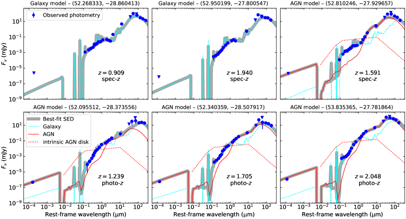
Figure 5: Example best-fit SED results for X-ray undetected (top row) and X-ray detected (bottom row) DOGs. All of the six sources have reliable redshifts (spec-$z$s or photo-$z$s with $Q_{z}^{\mathrm{good}}<1$, as shown in each panel). The blue points and downward triangles are the observed photometry and upper limits, respectively. The thick-grey lines are the best-fit total models. The cyan-dashed lines and the red-solid lines represent galaxy and AGN components, respectively. For sources where the statistically preferred model is the AGN model, we also show the intrinsic AGN disk SEDs, which are only modeled at $\lambda\geq 0.008\,\rm\mu m$ (Yang et al., 2022). The sharp peaks at rest-frame $<0.1\,\mathrm{\mu m}$ are strong nebular emission lines, as modeled by the templates from Inoue (2011). All sources shown with best-fit AGN models are classified as reliable SED AGNs. See Section 3 of Zou et al. (2022) for more details about our source classification. We also show the coordinates (RA and Dec) of each source at the top of each panel.

2.4 Distributions of $z$, $L_{\mathrm{bol}}$, and $L_{\mathrm{X,obs}}$

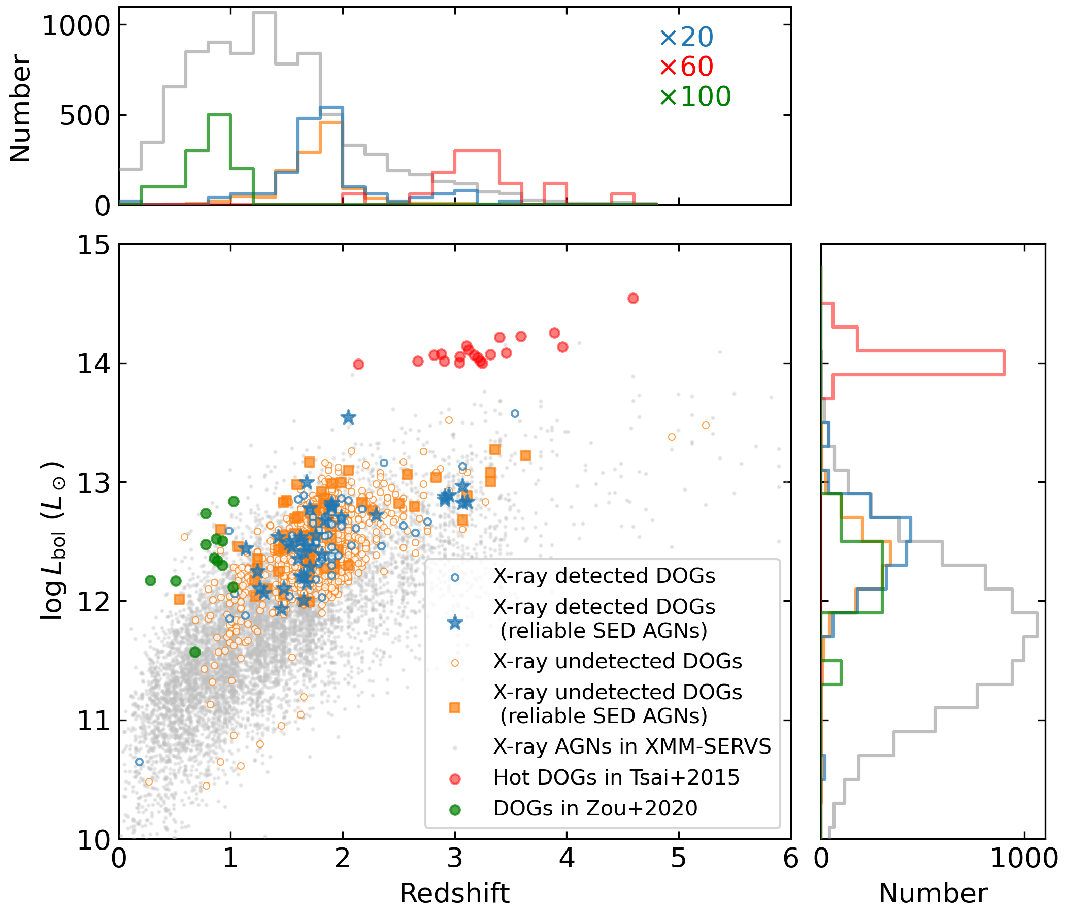
Figure 6: The $L_{\mathrm{bol}}$ versus $z$ distribution of our core sample. Our X-ray detected (undetected) DOGs are shown as blue (orange)-empty circles. Among them, sources classified as reliable SED AGNs in Zou et al. (2022) (see text in Section 3.1) are shown as filled stars for X-ray detected DOGs and filled squares for X-ray undetected DOGs. For comparison, the $L_{\mathrm{bol}}$ versus $z$ distributions of X-ray AGNs in XMM-SERVS, Hot DOGs in Tsai et al. (2015), and DOGs in Zou et al. (2020) are shown in grey, red, and green circles, respectively. The distributions of $z$ and $L_{\mathrm{bol}}$ for sources mentioned above are shown in the top and right subpanels, respectively, with the same colors as those in the legend (we do not further plot the distributions for our reliable SED AGNs). Note that for better visibility, in the top and right subpanels, the number of X-ray detected DOGs, Hot DOGs in Tsai et al. (2015), and DOGs in Zou et al. (2020) are multiplied by factors of 20, 60, and 100, respectively.

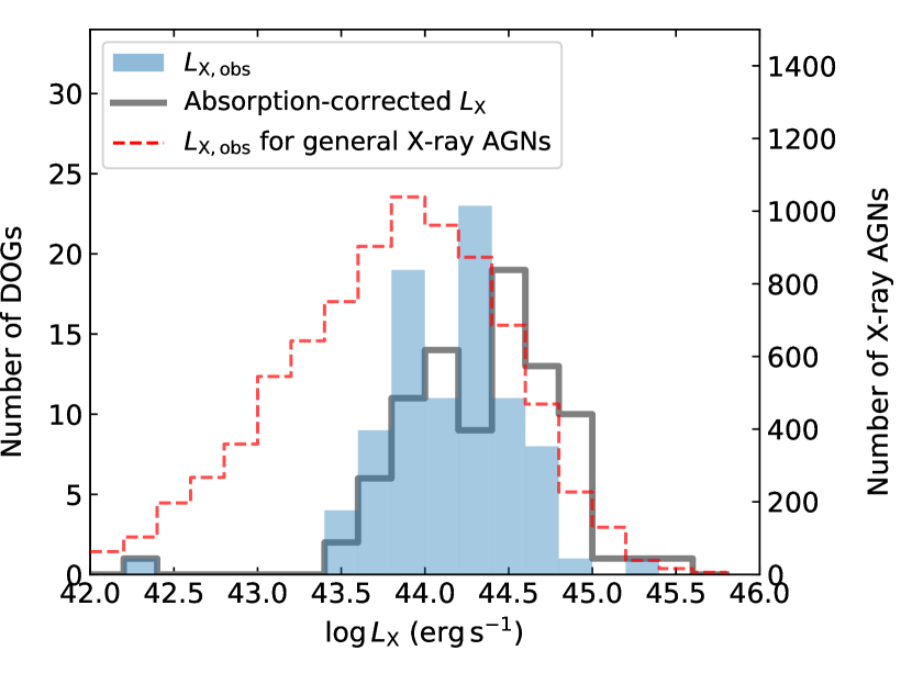
Figure 7: $L_{\mathrm{X,obs}}$ (blue) and absorption-corrected $L_{\mathrm{X}}$ (gray) distributions for X-ray detected DOGs in the core sample. The red-dashed histogram represents the $L_{\mathrm{X,obs}}$ distribution of general X-ray AGNs in XMM-SERVS. X-ray detected DOGs generally have high observed and absorption-corrected X-ray luminosity.

We calculate the $L_{\mathrm{bol}}$ for our samples using their best-fit SED models reported by Zou et al. (2022), where we integrate the total SED models from X-rays to FIR (observed-frame $10^{-4}-1000\,\mathrm{\mu m}$). Figure 6 shows the $L_{\mathrm{bol}}$ versus $z$ distribution for our core sample. The median redshift is $z=1.82$, and the $25-75\%$ quantile range is $z=1.63-1.93$. An AD test on X-ray detected and X-ray undetected DOGs returns a $p$-value of 0.06, indicating their redshift distributions are not significantly different. The median $\log L_{\mathrm{bol}}/L_{\sun}\approx 12.4$, and the $25-75\%$ quantile range is $\log L_{\mathrm{bol}}/L_{\sun}=12.3-12.6$. The results for our full sample are similar. For comparison, we also plot the distributions of general X-ray AGNs in XMM-SERVS (selected via $\mathtt{flag\_Xrayagn}=1$ from the SED catalog of Zou et al., 2022), Hot DOGs with $\log L_{\mathrm{bol}}/L_{\sun}>14$ in Tsai et al. (2015), and DOGs in Zou et al. (2020). DOGs selected by our criteria have a much narrower range of redshifts than typical X-ray AGNs. The narrow redshift distribution arises primarily because the $f_{\mathrm{24\mu m}}/f_{R}>982$ criterion selects against sources with lower redshifts. At our median $z\approx 1.8$, the observed $f_{\mathrm{24\mu m}}/f_{R}$ approximately corresponds to the rest-frame $8\,\mathrm{\mu m}$-to-2200 Å flux ratio. At lower redshifts, the observed $R$ band corresponds to redder rest-frame optical bands, which mitigates dust obscuration. The $L_{\mathrm{bol}}$ for our DOGs is much higher than that for X-ray AGNs, but is significantly lower than that for the most-extreme Hot DOGs. Given the low sky density ($\approx 1$ per $30\deg^{2}$; Wu et al., 2012) and the much higher $L_{\mathrm{bol}}$ of Hot DOGs than that for our sample, it is unlikely that our sample contains any extreme Hot DOGs. However, we can select lower-luminosity analogs to Hot DOGs using the best-fit SED models, and we present our results in Appendix B.

We also show the observed X-ray luminosity at rest-frame $2-10\,\rm keV$ ($L_{\mathrm{X,obs}}$) for X-ray detected DOGs in the core sample in Figure 7. For AGNs, the hard X-ray spectrum ($>2\,\mathrm{keV}$) is generally characterized by a power-law: $N(E)\propto E^{-\Gamma}$, where $N(E)$ is the photon number flux as a function of photon energy, and $\Gamma$ is the “intrinsic” power-law photon index. The intrinsic power-law photon index defines the spectral slope of the X-ray source, unaffected by any obscuring material (after correcting for Galactic absorption). For most AGNs, $\Gamma=1.7-2.2$ (e.g., Scott et al., 2011; Netzer, 2015; Liu et al., 2017). The “effective” power-law photon index ($\Gamma_{\mathrm{eff}}$), derived from a simple power-law fit, is a useful first-order descriptor of the spectral shape when the X-ray source is obscured (after correcting for Galactic absorption). For our DOGs, we assume a fixed effective power-law photon index of $\Gamma_{\mathrm{eff}}=1.4$ to allow for intrinsic absorption, and $L_{\mathrm{X,obs}}$ is calculated from the observed flux (corrected for Galactic but not intrinsic absorption) in one band based upon the following priority order: $2-10\,\rm keV$ (hard band; HB), $0.5-10\,\rm keV$ (full band; FB), $0.5-2\,\rm keV$ (soft band; SB) (Chen et al., 2018; Ni et al., 2021). This priority order is chosen to minimize absorption effects. An AD test on the full and core samples returns a $p$-value of 0.26, suggesting that the $L_{\mathrm{X,obs}}$ distributions are not significantly different between the two samples. For comparison, in Figure 7 we show the absorption-corrected $L_{\mathrm{X}}$ values which are derived using the $N_{\mathrm{H}}$ values in Section 3.2, and we show the $L_{\mathrm{X,obs}}$ for general X-ray AGNs in XMM-SERVS. Our DOGs are more luminous, with a median $L_{\mathrm{X,obs}}=10^{44.3}\,\mathrm{erg}\,\mathrm{s}^{-1}$. As our sources are at $z\approx 2$, the HB coverage roughly corresponds to $6-30\,\mathrm{keV}$ in the rest frame, which substantially mitigates any intrinsic obscuration.

3 Analyses and Results

In this section, we investigate several properties of our full and core samples. Section 3.1 presents the host-galaxy properties of our DOGs using the results from SED fitting. Section 3.2 investigates X-ray hardness ratios (HRs) and the corresponding $N_{\mathrm{H}}$. Section 3.3 presents X-ray stacking for X-ray undetected DOGs to assess their typical $L_{\mathrm{X,obs}}$ and $N_{\mathrm{H}}$. Section 3.4 shows the X-ray$-$MIR relation. In Section 3.5, we present radio properties.

3.1 Host-Galaxy Properties

The host-galaxy properties are derived from SED fitting, which decomposes the galaxy component and, if present, the AGN component.

SED fitting returns host-galaxy properties, including $M_{\star}$ and SFR. In general, $M_{\star}$ measurements should be robust, as they are determined mainly by SEDs at rest-frame $\approx 1\,\rm\mu m$ where the AGN component is often weaker than the galaxy component (e.g., Ciesla et al., 2015). For luminous type 1 AGNs, $M_{\star}$ is less reliable since the AGN component tends to dominate the emission from the UV to MIR. This should not impact our results significantly since there are only 3 reliable broad-line AGNs identified in Ni et al. (2021) in our full sample. We further check that, among our sources with best-fit AGN models, only $\approx 6\%$ and $\approx 2\%$ in the full and core samples have fractional flux contributions by the AGN at rest-frame $1\,\mathrm{\mu m}$ greater than $0.2$, respectively. We also compare our best-fit $M_{\star}$ with the $M_{\star}$ estimated using normal-galaxy templates ($M_{\star}^{\mathrm{gal}}$) in Appendix A, and the results are generally consistent. Thus, we conclude that our $M_{\star}$ measurements are not severely affected by AGN contributions. On the other hand, SFR measurements can incur more systematic uncertainties, but the inclusion of high-quality far-infrared (FIR) photometry can help obtain more reliable SFRs (e.g., Netzer et al., 2016). Among the five Herschel bands in the FIR, the Herschel SPIRE $250\,\mathrm{\mu m}$ photometry gives the highest fractions of DOGs with high-SNR measurements. There are $\approx 43\%$ of our X-ray detected DOGs and $\approx 54\%$ of our X-ray undetected DOGs having $\mathrm{SNR}>5$ at Herschel SPIRE $250\,\mathrm{\mu m}$. These fractions are also much higher than the typical fractions in XMM-SERVS. We also show that excluding FIR photometry will not cause significant biases in Appendix A.

Figure 8 shows the $M_{\star}$ distribution of our core sample, and the results for our full sample are similar. Our DOGs are generally massive galaxies (median $\log M_{\star}/M_{\sun}=11.0$, and the $25-75\%$ quantile range is $10.7-11.3$), which has also been noted by previous studies (e.g., Bussmann et al., 2012; Toba et al., 2015; Riguccini et al., 2019; Suleiman et al., 2022). Also, X-ray detected DOGs tend to have slightly higher $M_{\star}$ than X-ray undetected ones, which is confirmed by an AD test with a $p$-value $<0.001$. Indeed, AGNs tend to reside in massive galaxies, and black-hole accretion rates traced by X-ray luminosity monotonically increase as $M_{\star}$ increases (e.g., Yang et al., 2018; Zou et al., 2024).

Our DOGs generally have high SFRs (median $\mathrm{SFR}=141\,M_{\sun}\,\rm yr^{-1}$ and the $25-75\%$ quantile range is $65-277\,M_{\sun}\,\rm yr^{-1}$). Instead of showing SFR distributions, we use the normalized SFR ($\mathrm{SFR_{norm}}$) to represent how “starbursty” the source is compared with the SF main sequence (MS). $\mathrm{SFR_{norm}}$ is defined as $\mathrm{SFR}/\mathrm{SFR_{MS}}$, where $\mathrm{SFR_{MS}}$ is the MS SFR. We do not directly adopt the MS results from other literature works because they may have systematic offsets due to different methods of deriving $M_{\star}$ and SFR (e.g., Mountrichas et al., 2021). Thus, we use the SED catalogs in XMM-SERVS to calibrate the MS directly for our sources. Following Cristello et al. (2024), for each DOG, we select all galaxies within $\pm 0.1\,\rm dex$ in $M_{\star}$ and $\pm 0.075\times(1+z)$ in redshift. Among these matched galaxies, we select star-forming galaxies using their rest-frame $U-V$ and $V-J$ colors (i.e., the $UVJ$ diagram; e.g., Williams et al., 2009; Whitaker et al., 2012; Lee et al., 2018), which constitute a reference star-forming galaxy sample for the DOGs. We utilize the $UVJ$ selection criteria for star-forming galaxies in Zhang et al. (submitted), which were calibrated specifically for XMM-SERVS using the methods in Williams et al. (2009) and Whitaker et al. (2015). The adopted criteria are

$$U-V<1.3$$ (1)

as the horizontal cut, and

$$U-V >0.8\times(V-J)+0.84\ (0.0<z<0.5)$$ (2)

$$U-V >0.8\times(V-J)+0.83\ (0.5<z<1.0)$$

$$U-V >0.8\times(V-J)+0.75\ (1.0<z<1.5)$$

$$U-V >0.8\times(V-J)+0.72\ (1.5<z<2.5)$$

$$U-V >0.8\times(V-J)+0.70\ (z>2.5)$$

as the diagonal cut. Most of the sources in the catalog are identified as normal galaxies, and only $\approx 3\%$ are identified as AGNs by Zou et al. (2022). Thus, our selection should not be materially impacted by AGNs. We use the median SFR of the selected star-forming galaxies as the $\rm SFR_{MS}$ of the corresponding DOG, and apply the above steps for all our DOGs. In principle, one must consider the mass-completeness limit, as the determination of the MS may be biased. However, since our sources generally have high $M_{\star}$ with only $\approx 3\%$ below the mass-completeness curves for XMM-SERVS (see Section 2.4 of Zou et al., 2024), we do not further apply a mass-completeness cut, and the results should not be significantly impacted. One caveat in the determination of the MS is that star-forming galaxies cannot be reliably distinguished at high-$M_{\star}$ and/or low-$z$ due to the high fraction of quiescent or transitioning galaxies in those regimes, where the classification of star-forming galaxies (and, consequently, the determination of $\mathrm{SFR_{MS}}$) may become sensitive to the adopted methods (e.g., Donnari et al., 2019). Cristello et al. (2024) proposed a redshift-dependent maximum $M_{\star}$ for reliable classifications using the following procedures. For each AGN in their sample, they selected all galaxies within $\pm 0.1\,\rm dex$ in $M_{\star}$ and $\pm 0.075\times(1+z)$ in redshift. Among these reference galaxies, they classified star-forming and quiescent galaxies using the method in Tacchella et al. (2022). The regime in the $z-M_{\star}$ plane where the fraction of quiescent galaxies is less than 0.5 was determined to be the “safe” regime. The maximum $M_{\star}$ for the “safe” regime can be well described at $z=0.1-4$ by the following equation:

$$\log M_{\star}=10.65+0.81\log z+0.38\log(1+z).$$ (3)

The “safe” regime is established to minimize MS offsets when probing the highest masses, ensuring that $\mathrm{SFR_{MS}}$ remains similar regardless of different MS definitions. We adopt Equation 3 to determine our “safe” DOGs.

$\mathrm{SFR_{norm}}$ has three sources of uncertainty: SFR, $M_{\star}$, and the determination of the MS. The systematic bias in how we determine the MS is generally not significant as long as we measure the SFRs for our DOGs and reference galaxies self-consistently and calibrate the MS. Furthermore, the MS uncertainty is also small for our “safe” sample as it is constructed to minimize MS offsets. The relative uncertainty of $M_{\star}$ is also generally smaller than that of SFR, so the $\mathrm{SFR_{norm}}$ uncertainty is primarily driven by the SFR uncertainty of our DOGs. Our typical SFR uncertainty is $\lesssim 0.3\,\rm dex$, which is generally acceptable for SED fitting.

Figure 9 shows the $\mathrm{SFR_{norm}}$ distribution for our core sample, with the “safe” sources in solid lines, as well as all sources, including the “unsafe” ones, in dashed lines. An AD test comparing the distributions of the “safe” and all sources returns a $p$-value of 0.06 for X-ray undetected DOGs, and 0.99 for X-ray detected DOGs, showing that the $\mathrm{SFR_{norm}}$ distributions of the “safe” and all sources are not significantly different. This implies that our MS definition is generally reliable even for high-$M_{\star}$ and/or low-$z$ galaxies. Considering all the sources in the core sample, we find X-ray detected DOGs have a higher fraction of sources below the MS (32% with $\log\mathrm{SFR_{norm}}<-0.4$), while the X-ray undetected ones are generally on or above the MS (only 8% with $\log\mathrm{SFR_{norm}}<-0.4$). An AD test returns a $p$-value $<0.001$ when comparing the X-ray detected and undetected sources, confirming that they have different $\mathrm{SFR_{norm}}$ distributions. The difference may be caused by selection effects for our color-based selection criteria, as discussed in 2.3, where X-ray detected DOGs may be biased toward higher fractional FIR flux contributions from AGNs, which results in reduced levels of SFR from the galaxy component. We will further discuss how the $\mathrm{SFR_{norm}}$ distributions of X-ray detected DOGs compare with matched typical X-ray AGNs in Section 4.2.

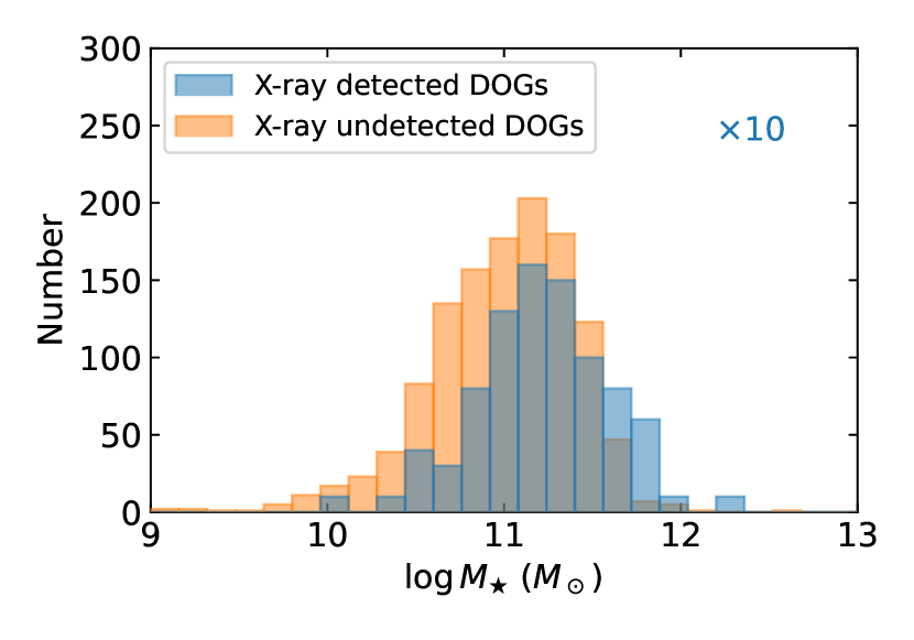
Figure 8: $M_{\star}$ distribution for the core sample. Blue and orange histograms represent X-ray detected and X-ray undetected DOGs, respectively. Note that the number of X-ray detected DOGs in each bin is multiplied by a factor of 10 for easier visibility. DOGs generally have high $M_{\star}$, and X-ray detected DOGs have slightly higher $M_{\star}$. The distributions for our full sample are similar.

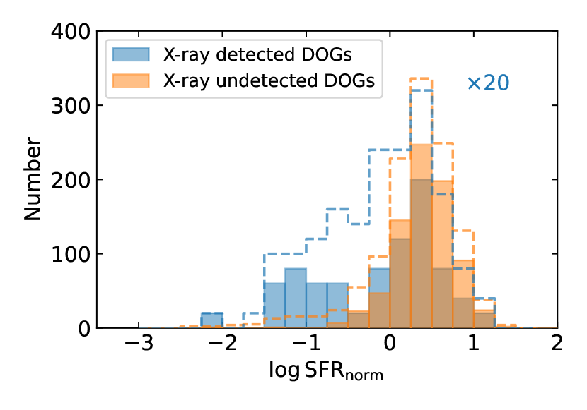
Figure 9: $\rm SFR/SFR_{MS}$ distribution for the core sample. Blue and orange histograms represent X-ray detected DOGs and X-ray undetected DOGs, respectively. Solid histograms represent the “safe” sources where the corresponding star-forming MS can be reliably obtained. Dashed histograms represent all the sources in our sample. Note that the number of X-ray detected DOGs in each bin is multiplied by a factor of 20 for easier visibility. X-ray detected DOGs have a higher fraction of sources below the MS. The distributions for our full sample are similar.

3.2 HRs and $N_{\mathrm{H}}$

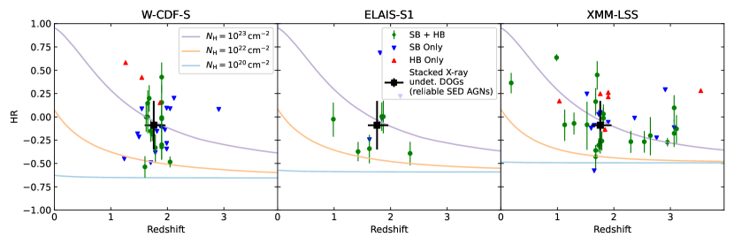
Figure 10: HR versus redshift in W-CDF-S (left), ELAIS-S1 (middle), and XMM-LSS (right) for the core sample. The colored points are our X-ray detected DOGs, and the legend in the middle panel indicates their detection status in the SB and HB. Green points with error bars represent the median HR values with $1\sigma$ uncertainties for sources detected in both bands. The blue downward triangles, which are detected in the SB but not the HB, represent $1\sigma$ HR upper limits. The red upward triangles, which are detected in the HB but not the SB, are $1\sigma$ HR lower limits. The black squares represent stacked X-ray undetected DOGs that are classified as reliable SED AGNs in the core sample (see Section 3.3), with the error bar in the $x$-axis direction showing the $25-75\%$ redshift quantile range. The solid lines are the expected relations for redshifted absorbed power-laws, whose intrinsic photon index $\Gamma=1.8$, with several different $N_{\mathrm{H}}$ values, as labeled in the legend.

In this subsection, we investigate the basic X-ray spectral properties of our X-ray detected DOGs. Given the limited counts (typically $90-200$ in the FB), we are not able to perform detailed X-ray spectral fitting for most of our DOGs detected in X-rays. We thus analyze the HRs for simplicity to probe their spectral properties. HR is defined as $(\mathrm{CR}_{\mathrm{H}}-\mathrm{CR}_{\mathrm{S}})/(\mathrm{CR}_{\mathrm{H}}+\mathrm{CR}_{\mathrm{S}})$, where $\mathrm{CR}_{\mathrm{H}}$ and $\mathrm{CR}_{\mathrm{S}}$ represent the HB and SB count rates, respectively. The cataloged HRs in XMM-SERVS are reliable mainly for sources detected in both the SB and HB, but many of our sources are detected only in one band. In particular, possible high $N_{\mathrm{H}}$ values present in DOGs can severely impact the detection in the SB while not affecting the HB too much. We thus apply a Bayesian method described in Appendix A of Zou et al. (2023) to calculate the HRs for our X-ray detected DOGs. We also calculate the expected $z-\mathrm{HR}$ curves in each field, assuming an absorbed power-law with intrinsic photon index $\Gamma=1.8$. These curves are calculated using the Portable Interactive Multi-Mission Simulator (PIMMS). In brief, given a spectral model, we first obtain the net count rates for a given band (SB and HB) in a given instrument (PN, MOS1, and MOS2) as a function of redshift. Then, we weigh the count rates by the median exposure times of each instrument in each band across the field to calculate the HRs (assuming intrinsic $\Gamma=1.8$) at different redshifts. It is worth noting that using standard photoelectric absorption to calculate spectral shape is appropriate up to $N_{\mathrm{H}}\approx 10^{23.5}\,\mathrm{cm}^{-2}$; when $N_{\mathrm{H}}\gtrsim 10^{24}\,\mathrm{cm}^{-2}$ (i.e., CT absorption), the reflection component from the torus and other effects may become prominent.

We present the results for our core sample in Figure 10, along with the expected $z-\mathrm{HR}$ curves at different $N_{\mathrm{H}}$ values. Our X-ray detected DOGs generally have $N_{\mathrm{H}}>10^{22}\,\mathrm{cm}^{-2}$ except for several sources, and a large fraction of them reach $N_{\mathrm{H}}>10^{23}\,\mathrm{cm}^{-2}$. Among 174 X-ray detected sources in our full sample, 87 have $N_{\mathrm{H}}>10^{23}\,\mathrm{cm}^{-2}$; 43 out of 88 X-ray detected sources in the core sample have $N_{\mathrm{H}}>10^{23}\,\mathrm{cm}^{-2}$. These fractions are similar to X-ray spectral fitting results for DOGs in the ultradeep CDF-S field, where they found $\approx 64\%$ of X-ray detected DOGs with $N_{\mathrm{H}}>10^{23}\,\mathrm{cm}^{-2}$ (Corral et al., 2016).

The calculated HRs can be further converted to $N_{\mathrm{H}}$ values by interpolating over the $z-\mathrm{HR}$ curves at different obscuration levels. The median $N_{\mathrm{H}}$ for our core sample is $10^{22.8}\,\mathrm{cm}^{-2}$. Recently, Kayal & Singh (2024) and Cristello et al. (submitted) both performed X-ray spectral analyses for X-ray detected DOGs with sufficient counts in XMM-SERVS. The former covered XMM-LSS, while the latter covered all three XMM-SERVS fields. Note that Kayal & Singh (2024) used the HSC Subaru Strategic Program and the SWIRE band-merged catalogs as their parent sample to select DOGs, while Cristello et al. (submitted) utilized our DOG catalog directly. We compare our HR-derived $N_{\mathrm{H}}$ with the results from X-ray spectral fitting in Figure 11. Our $N_{\mathrm{H}}$ values appear systematically higher in general than those estimated via X-ray spectral analyses, which should be kept in mind for the following discussion. Figure 12 shows the absorption-corrected rest-frame $2-10\,\mathrm{keV}$ $L_{\mathrm{X}}$ versus $N_{\mathrm{H}}$ for our X-ray detected DOGs as well as other AGN populations collected from the literature: reddened type 1 quasars (Urrutia et al., 2005; Martocchia et al., 2017; Mountrichas et al., 2017; Goulding et al., 2018; Lansbury et al., 2020), SMGs (Wang et al., 2013), DOGs (Lanzuisi et al., 2009; Corral et al., 2016; Zou et al., 2020), and Hot DOGs (Stern et al., 2014; Assef et al., 2016; Ricci et al., 2017; Vito et al., 2018). We use the derived $N_{\mathrm{H}}$ from our HR results to correct for the intrinsic absorption using sherpa. The correction factor is generally modest (median value of $\approx 1.9$) because, at the median redshift of our sources, the HB corresponds to rest-frame $\approx 6-30\,\mathrm{keV}$, which is not significantly affected by absorption at the observed levels. Our $N_{\mathrm{H}}$ values span a wide range and are generally consistent with those for DOGs in previous studies. Our X-ray detected DOGs also show slightly higher $L_{\mathrm{X}}$, which is mostly due to the wide homogeneous medium-deep X-ray coverage of XMM-SERVS that allows us to select more luminous sources compared with previous studies in small ultra-deep fields (e.g., Corral et al., 2016).

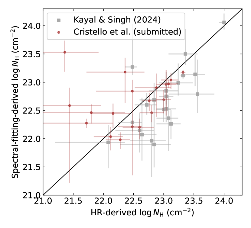
Figure 11: Comparison between our HR-derived $N_{\mathrm{H}}$ values and those derived from X-ray spectral fitting. The grey squares represent the results from Kayal & Singh (2024). The brown circles represent the results from Cristello et al. (submitted). The error bars represent $1\sigma$ uncertainties.

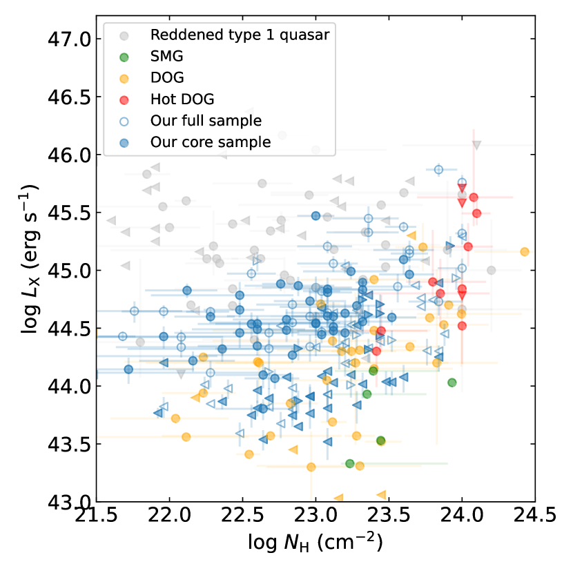
Figure 12: Comparison between our samples and previous studies in the $N_{\mathrm{H}}-L_{\mathrm{X}}$ plane. The $N_{\mathrm{H}}$ values of our DOGs are converted from their HRs. The blue points are our X-ray DOGs detected in both SB and HB with $1\sigma$ confidence error bars; the blue leftward and rightward triangles represent X-ray DOGs detected only in HB or SB ($1\sigma$ lower/upper limits for $N_{\mathrm{H}}$), respectively. Our full and core samples are indicated by empty and filled symbols, respectively. The grey, green, yellow, and red points are reddened type 1 quasars, SMGs, DOGs, and Hot DOGs from previous studies, respectively (see the text for sample references). Our X-ray detected DOGs are luminous with a wide range of obscuration.

3.3 X-ray Stacking

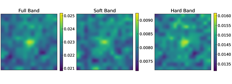
Figure 13: Smoothed stacked X-ray images combining all three EPIC cameras for our core-sample DOGs that are away from known X-ray sources (647 in total) in the FB, SB, and HB. Each image has a size of $60\arcsec\times 60\arcsec$. The numbers on the color bars are in units of $\rm count\,s^{-1}$.

X-ray stacking allows for the detection, on average, of sources lying below the formal detection limits (e.g., Vito et al., 2016). In this subsection, we stack the X-ray images of our X-ray undetected DOGs to study their X-ray properties further. We select DOGs at least 52$\arcsec$ away from all the X-ray sources to avoid contamination, which results in the selection of about 50% of the sources. We restrict our stacking to regions where the total FB exposure from all three EPIC cameras $>14\,\rm ks$ in W-CDF-S, $>10\,\rm ks$ in ELAIS-S1, and $>25\,\rm ks$ in XMM-LSS, which constitute $\approx 95\%$ of the area covered in X-rays. This step removes pixels with low exposures that may adversely affect the count-rate calculations. We also restrict the stacking for the other bands to the same regions. We end up with 1825 sources in the full sample and 647 in the core sample. We then extract the combined count-rate maps from all three EPIC cameras in all three X-ray bands within a $60\arcsec\times 60\arcsec$ region around each selected source and sum the maps to obtain the stacked image. Figure 13 shows the smoothed stacked images of X-ray undetected DOGs in the FB, SB, and HB for our core sample. The stacked signal is prominent in all three bands visually. To further assess the false-detection probabilities, we perform Monte Carlo stacking analyses (e.g., Brandt et al., 2001).

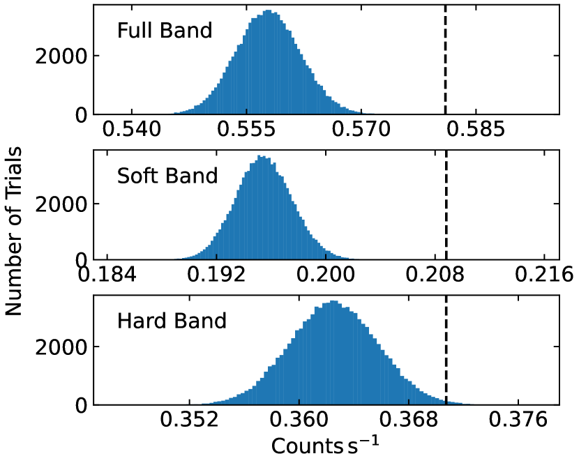
Figure 14: Results from our Monte Carlo X-ray stacking for the core sample. For each plot, we perform 100000 stacking trials at random positions around the undetected sources. The vertical dashed lines represent the stacked count rates at the positions of the undetected sources. In all three bands, we have significant detections. The results for our full sample are similar.

The Monte Carlo stacking analyses are performed for the 1825/647 X-ray undetected DOGs in the full/core sample that are free from contamination and low-exposure regions. For our core sample, we stack 647 images using a $20\arcsec\times 20\arcsec$ aperture ($5\times 5$ pixels) at the position of each source to obtain the stacked source count rates. The aperture is chosen to be consistent with our calculations of count rates and flux in the next paragraph. We further perform local background stacking with 100000 trials, where we stack 647 random positions using the same aperture. These random positions are chosen to lie in an annular region (with an inner radius of $1\arcmin$ and an outer radius of $2\arcmin$) centered on each source (avoiding known X-ray sources) to reproduce the actual background distribution as closely as possible. The stacked exposure reaches $\approx 55\,\rm Ms$, enabling the average detection below our survey sensitivity. We repeat the above procedure for all three bands and show the results for our core sample in Figure 14. In all three bands, the resulting background distributions are nearly Gaussian. There are 0/0/573 out of 100000 trials in the FB/SB/HB with background count rates higher than the stacked source count rates. This corresponds to a false-detection level ($P_{\mathrm{false}}$) of $<10^{-5}$ for the FB and the SB, and $0.00573$ for the HB, indicating significant detections in all three bands. The results for our full sample are similar.

We further calculate the count rates within the $5\times 5$-pixel aperture and net source fluxes using the single-camera exposure ($t$) maps, encircled-energy fraction (EEF) maps, and energy-conversion factors (ECFs) in Chen et al. (2018) and Ni et al. (2021), where EEF is the expected fraction of source counts falling within the given aperture centered at the source position, and ECF is the expected ratio between the source flux and source counts. The $5\times 5$-pixel aperture is chosen to be consistent with the EEF maps derived in Chen et al. (2018) and Ni et al. (2021). We apply the same procedures as in our Monte Carlo count analyses to derive the stacked count rates and background count-rate distributions. The background count-rate distributions are also nearly Gaussian. Following Ruiz et al. (2022), we convert the stacked net count rates to fluxes in each band using

$$f_{\mathrm{X}}=S\sum^{N}\sum_{i=1}^{3}t_{i}/\sum^{N}\sum_{i=1}^{3}t_{i}\,\mathrm{EEF}_{i}\,\mathrm{ECF}_{i},$$ (4)

where $S$ denotes the stacked net count rates within $5\times 5$ pixels, $f_{\mathrm{X}}$ denotes the derived X-ray flux, $i$ denotes the cameras (PN, MOS1, and MOS2), and $N$ denotes the number of stacked sources. The stacking results are summarized in Table 5. For the 647 sources stacked in the core sample, after correction for Galactic absorption, the average observed HB net flux ($f_{\mathrm{X}}^{\mathrm{HB}}$) is $(3.3\pm 1.3)\times 10^{-16}\,\mathrm{erg}\,\mathrm{cm}^{-2}\,\mathrm{s}^{-1}$. Assuming an effective power-law photon index of $\Gamma_{\mathrm{eff}}=1.4$, the median $L_{\mathrm{X,obs}}$ at rest-frame $2-10\,\mathrm{keV}$ is $(4.3\pm 1.7)\times 10^{42}\,\mathrm{erg}\,\mathrm{s}^{-1}$. The results for our full sample are similar. We also have verified that our X-ray stacking procedure does not have significant biases by stacking X-ray detected sources with known X-ray flux.

We further estimate the non-AGN X-ray emission from host galaxies to assess if the stacked X-ray emission is sufficiently strong to indicate the presence of AGNs. X-ray emission from host galaxies is expected to primarily comes from X-ray binaries (XRBs) and hot gas. Following the same procedure as in Section 2.2 of Zou et al. (2023), we adopt the scaling relation in Lehmer et al. (2016) to estimate the total HB flux from low-mass XRBs and high-mass XRBs assuming an intrinsic power-law photon index of 1.8, and the scaling relation in Kim & Fabbiano (2015) to estimate the X-ray emission from hot gas. We then apply K-corrections using sherpa (Freeman et al., 2001; Doe et al., 2007) to convert the hot-gas $L_{\mathrm{X}}$ to the HB flux using the hot-gas spectra, with the gas temperature given by the scaling relation. For our core sample, the average $f_{\mathrm{X}}^{\mathrm{HB}}$ estimated from stacking is 3.8 times higher than the estimated average flux ($8.6\times 10^{-17}\,\mathrm{erg}\,\mathrm{cm}^{-2}\,\mathrm{s}^{-1}$) contributed by XRBs and hot gas. The results for our full sample are similar. The observed HB flux is much higher than the predicted values from non-AGN contributions, proving the presence of AGNs among our X-ray undetected DOGs.

Among X-ray undetected DOGs, objects can be classified into three categories following Section 3.5 of Zou et al. (2022): reliable SED AGNs, AGN candidates but not reliable SED AGNs, and normal galaxies (see Section 3.1). We further stack these three subsets separately to see if our SED-based classification truly reflects the contribution of AGNs. Among the 647 sources in the core sample, 37 are reliable SED AGNs, 191 are AGN candidates but not reliable SED AGNs, and 419 are normal galaxies. We use the same procedures as described earlier in this subsection to stack these subsets.

The stacking results are summarized in Table 5. We have checked that the stacked count rates are not dominated by any individual source. The results show that sources classified as AGN candidates indeed have more significant X-ray detections. We find the subsets for reliable SED AGNs produce the highest average $L_{\mathrm{X,obs}}$ at rest-frame 2–10 $\mathrm{keV}$, while no detections are found for normal galaxies in the HB. AGN candidates also show slightly elevated HR compared to X-ray undetected DOGs in general, which may be because normal galaxies contribute more to the SB count rates than to the HB. In fact, we have verified that both the predicted SB flux and HB flux for normal galaxies are consistent with the total XRB and hot-gas emission predicted by Lehmer et al. (2016) and Kim & Fabbiano (2015). Thus, the HR of our AGN candidates is more representative of the obscuration in the nuclear region. We also plot the HR for our stacked reliable SED AGNs in Figure 10. On average, our X-ray undetected AGN candidates have $N_{\mathrm{H}}\gtrsim 10^{23}\,\mathrm{cm}^{-2}$, which is consistent with or slightly higher than the median value of $N_{\mathrm{H}}=10^{22.8}\,\mathrm{cm}^{-2}$ for our X-ray detected DOGs.

We further calculate the total rest-frame 2–10 $\mathrm{keV}$ $L_{\mathrm{X,obs}}$ ($L_{\mathrm{X,obs}}^{\mathrm{tot}}$) of each stacked subset to probe their overall accretion power, assuming that each source contributes equally to the total $f_{\mathrm{X}}^{\mathrm{HB}}$. The total accretion power can be traced by the total intrinsic $L_{\mathrm{X}}$. For X-ray undetected DOGs, we assume that every source is obscured at the average obscuration level of $N_{\mathrm{H}}=10^{23}\,\mathrm{cm}^{-2}$ as shown in the previous paragraph. We then use PIMMS to convert the $L_{\mathrm{X,obs}}$ to intrinsic $L_{\mathrm{X}}$. The correction is generally small ($\approx 5-10\%$) as the HB corresponds to $\approx 6-30\,\mathrm{keV}$ in the rest frame at the median redshift of our sources. We also use the intrinsic $L_{\mathrm{X}}$ derived in Section 3.2 to assess the accretion power contributed by X-ray detected DOGs. We find the total accretion power for our DOGs is dominated by X-ray detected sources, which contribute $\approx{75\%}$ of the total intrinsic $L_{\mathrm{X}}$ for our core sample. Even in the extreme case where all the stacked X-ray undetected DOGs are heavily obscured at $N_{\mathrm{H}}\approx 10^{24}\,\mathrm{cm}^{-2}$, the correction factor for their total $L_{\mathrm{X}}$ would only be $\approx 1.5$, which will not significantly impact our results. The results are consistent with previous measurements and/or simulations of SMBH growth, which conclude that most SMBH growth occurs in luminous AGNs (e.g., Brandt & Alexander, 2015; Vito et al., 2016; Volonteri et al., 2016; Zou et al., 2024).

Table 5: X-ray stacking results for subsamples of X-ray undetected DOGs.

Subsample	$N$	$P_{\mathrm{false}}^{\mathrm{SB}}$	$\mathrm{CR}_{\mathrm{S}}$	$P_{\mathrm{false}}^{\mathrm{HB}}$	$\mathrm{CR}_{\mathrm{H}}$	Hardness ratio	$f_{\mathrm{X}}^{\mathrm{HB}}$	$L_{\mathrm{X,obs}}$	$L_{\mathrm{X,obs}}^{\mathrm{tot}}$
(1)	(2)	(3)	(4)	(5)	(6)	(7)	(8)	(9)	(10)
Full Sample
All	1825	$10^{-5}$	$2.11\pm 0.21$	$<10^{-5}$	$1.70\pm 0.31$	$-0.11\pm 0.10$	$4.5\pm 0.8$	$0.62\pm 0.11$	$18.3\pm 3.2$
Reliable SED AGNs	171	0.00158	$4.06\pm 0.76$	$<10^{-5}$	$4.50\pm 1.12$	$0.05\pm 0.16$	$12.4\pm 3.1$	$3.2\pm 0.8$	$\phantom{p}8.1\pm 2.0$
AGN candidates but not reliable	694	$<10^{-5}$	$2.47\pm 0.34$	$<10^{-5}$	$2.61\pm 0.51$	$0.03\pm 0.12$	$7.0\pm 1.4$	$1.12\pm 0.22$	$14.7\pm 2.9$
Normal galaxies	960	$<10^{-5}$	$1.51\pm 0.29$	$0.12963$	$0.54\pm 0.41$	…	…	…	…
Core Sample
All	647	$<10^{-5}$	$2.06\pm 0.32$	$0.00083$	$1.27\pm 0.50$	$-0.24\pm 0.18$	$3.3\pm 1.3$	$0.43\pm 0.17$	$2.7\pm 1.1$
Reliable SED AGNs	37	$0.04796$	$6.47\pm 1.45$	$0.00057$	$5.34\pm 2.60$	$-0.09\pm 0.26$	$14.5\pm 7.0$	$1.7\pm 0.8$	$0.8\pm 0.4$
AGN candidates but not reliable	191	$0.00038$	$2.10\pm 0.57$	$0.00121$	$2.70\pm 0.89$	$0.13\pm 0.22$	$7.3\pm 2.3$	$0.83\pm 0.26$	$1.8\pm 0.6$
Normal galaxies	419	$0.00005$	$1.65\pm 0.40$	$0.34431$	$0.24\pm 0.61$	…	…	…	…

Note. — Our stacking utilizes X-ray images from all three EPIC cameras. We only show hardness ratio, flux, $L_{\mathrm{X,obs}}$, and $L_{\mathrm{X,obs}}^{\mathrm{tot}}$ when a detection of $>2\sigma$ ($P_{\mathrm{false}}<0.05$) is achieved. Column (1): Subsamples of X-ray undetected DOGs based upon the SED classification results. Column (2): Number of sources stacked. Column (3): Fraction of trials with stacked background count rates higher than the stacked count rate at the position of the source in the SB. Column (4): Average net count rate within a $20\arcsec\times 20\arcsec$ aperture in the SB in units of $10^{-5}$ $\rm counts\,s^{-1}$. Column (5): Fraction of trials with stacked background count rates higher than the stacked count rate at the position of the source in the HB. Column (6): Average net count rate within a $20\arcsec\times 20\arcsec$ aperture in the HB in units of $10^{-5}$ $\rm counts\,s^{-1}$. Column (7): Hardness ratio. Column (8): Galactic absorption-corrected average observed net flux in the HB in units of $10^{-16}\,\mathrm{erg}\,\mathrm{cm}^{-2}\,\mathrm{s}^{-1}$. Column (9): Observed X-ray luminosity at rest-frame 2–10 $\mathrm{keV}$ in units of $10^{43}\,\mathrm{erg}\,\mathrm{s}^{-1}$ using the median redshift of each subset, calculated from the Galactic absorption-corrected average net HB flux assuming $\Gamma_{\mathrm{eff}}=1.4$. Column (10): The total rest-frame 2–10 $\mathrm{keV}$ $L_{\mathrm{X,obs}}$ in units of $10^{45}\,\mathrm{erg}\,\mathrm{s}^{-1}$ contributed by each subset.

3.4 $L_{\mathrm{X,obs}}$ versus $L_{\mathrm{6\mu m,AGN}}$

The MIR continuum luminosity is a robust indicator of the intrinsic AGN strength, as MIR emission is largely unaffected by obscuration except for the most extreme obscuration levels ($A_{V}\approx 30$; e.g., Stern, 2015), while our sources are much below such levels. Many studies have shown a tight relationship between the absorption-corrected $L_{\mathrm{X}}$ and the rest-frame $6\,\rm\mu m$ continuum luminosity contributed by AGNs ($\nu L_{\nu}^{\mathrm{AGN}}$, written as $L_{\mathrm{6\mu m,AGN}}$ hereafter; e.g., Fiore et al., 2009; Lanzuisi et al., 2009; Stern, 2015; Chen et al., 2017). Since $L_{\mathrm{X,obs}}$ for AGNs will be significantly suppressed when $N_{\mathrm{H}}$ is sufficiently large, comparing $L_{\mathrm{X,obs}}$ versus $L_{\mathrm{6\mu m,AGN}}$ with the nominal absorption-corrected $L_{\mathrm{X}}-L_{\mathrm{6\mu m,AGN}}$ relation can be helpful to identify heavily-obscured and CT AGNs (e.g., Rovilos et al., 2014; Lanzuisi et al., 2018; Guo et al., 2021; Yan et al., 2023).

The $L_{\mathrm{6\mu m,AGN}}$ and its uncertainty are derived from the CIGALE SED-fitting output agn.L_6um. It is worth noting that the rest-frame $6\,\mathrm{\mu m}$ luminosity utilized here should be solely contributed from AGNs. At the redshift range of our DOGs ($z\approx 1.5-2.5$), rest-frame $6\,\rm\mu m$ corresponds to $15-20\,\rm\mu m$ in the observed frame. Since our sources have high $24\,\rm\mu m$ fluxes by construction, and all sources have at least one photometric band with $\rm SNR>5$ at $4.5\,\mathrm{\mu m}$, $5.8\,\mathrm{\mu m}$, or $8\,\mathrm{\mu m}$, the measurements of $L_{\mathrm{6\mu m,AGN}}$ should be reliable as long as the emission at rest-frame $6\,\mathrm{\mu m}$ is dominated by AGNs (i.e., small galaxy contamination; Yang et al., 2020). We calculate the AGN fractional flux contribution at rest-frame $6\,\mathrm{\mu m}$ using the CIGALE output agn.fracAGN with lambda_fracAGN set to “6/6” (Yang et al., 2022). Around 90% of AGN candidates among our DOGs have an AGN fractional contribution $>50\%$, indicating the $L_{\mathrm{6\mu m,AGN}}$ measurements should be reliable.

We plot $L_{\mathrm{X,obs}}$ versus $L_{\mathrm{6\mu m,AGN}}$ for our X-ray detected DOGs in the top panel of Figure 15. We also show the absorption-corrected $L_{\mathrm{X}}-L_{\mathrm{6\mu m,AGN}}$ relation in Stern (2015) along with the $1\sigma$ and $3\sigma$ dispersions of their sample. Most X-ray detected DOGs lie within the $1\sigma$ dispersion, although they generally show slightly suppressed $L_{\mathrm{X,obs}}$ and some are below the $1\sigma$ dispersion range. Such deviations are likely due to obscuration as described in Section 3.2. We plot the absorption-corrected $L_{\mathrm{X}}$ versus $L_{\mathrm{6\mu m,AGN}}$ in the bottom panel of Figure 15, and most of our X-ray detected DOGs are now consistent with the Stern (2015) relation and do not show obvious systematic offsets. We further show the stacked average $L_{\mathrm{X,obs}}$ versus the median $L_{\mathrm{6\mu m,AGN}}$ for X-ray undetected reliable SED AGNs in our core sample (marked with a black square) in the top panel of Figure 15. As all reliable SED AGNs have AGN fractional flux contribution $>50\%$ at rest-frame 6$\mathrm{\mu m}$, their median $L_{\mathrm{6\mu m,AGN}}$ should be reliable. On average, reliable SED AGNs are $\approx 3\sigma$ ($\approx 1.5\,\rm dex$) below the $L_{\mathrm{X,obs}}-L_{\mathrm{6\mu m,AGN}}$ relation. We calculate the expected line-of-sight $N_{\mathrm{H}}$ value corresponding to such a low $L_{\mathrm{X,obs}}/L_{\mathrm{6\mu m,AGN}}$ using photoelectric absorption with Compton-scattering losses, and obtain $N_{\mathrm{H}}\approx 10^{24}\,\mathrm{cm}^{-2}$. This value is much larger than the HR-derived $N_{\mathrm{H}}$ of $\approx 10^{23}\,\mathrm{cm}^{-2}$ in Section 3.3 and Figure 10. There are two main reasons for this discrepancy. First, our HR-derived $N_{\mathrm{H}}$ does not consider a possible soft scattered component. A soft scattered component is often observed in the soft X-ray band of AGNs. For obscured AGNs, this component is likely a power-law scattered back into the line of sight, and it generally has $<10\%$ of the flux of the primary power-law (e.g., Guainazzi & Bianchi, 2007; Brightman & Ueda, 2012). The presence of the soft scattered component will lead to an underestimated $N_{\mathrm{H}}$ based upon HR. Second, $L_{\mathrm{X,obs}}/L_{\mathrm{6\mu m,AGN}}$ is not solely determined by $N_{\mathrm{H}}$. Physical modeling shows that $L_{\mathrm{X,obs}}/L_{\mathrm{6\mu m,AGN}}$ may also be sensitive to AGN torus covering fraction and the incident X-ray continuum shape (Murphy & Yaqoob, 2009); observations have also shown that AGNs with higher $f_{\mathrm{24\mu m}}/f_{R}$ have lower $L_{\mathrm{X,obs}}/L_{\mathrm{6\mu m,AGN}}$ (up to $1\,\rm dex$ difference) when their $N_{\mathrm{H}}$ values are similar to AGNs with lower $f_{\mathrm{24\mu m}}/f_{R}$ (e.g., see Figure 8 in Li et al., 2020). Our DOGs indeed have high $f_{\mathrm{24\mu m}}/f_{R}$ by construction, so the $N_{\mathrm{H}}$ derived from the deviation from the absorption-corrected $L_{\mathrm{X}}-L_{\mathrm{6\mu m,AGN}}$ relation may be overestimated. This effect may also partly explain why there are several X-ray detected DOGs slightly below the Stern (2015) relation after absorption correction.

Apart from these two effects, it is also possible that galaxy contamination in the SB among our reliable SED AGNs results in a lower HR, as the purity of the reliable SED AGNs is $\gtrsim 75\%$ (see Section 3.1). However, we have verified that galaxy contamination is generally small and should not cause significant differences in our HRs. Nevertheless, the significantly lower $L_{\mathrm{X,obs}}/L_{\mathrm{6\mu m,AGN}}$ for X-ray undetected reliable SED AGNs than those for X-ray detected DOGs implies that AGNs among X-ray undetected DOGs have heavier obscuration, and some may even reach CT levels.

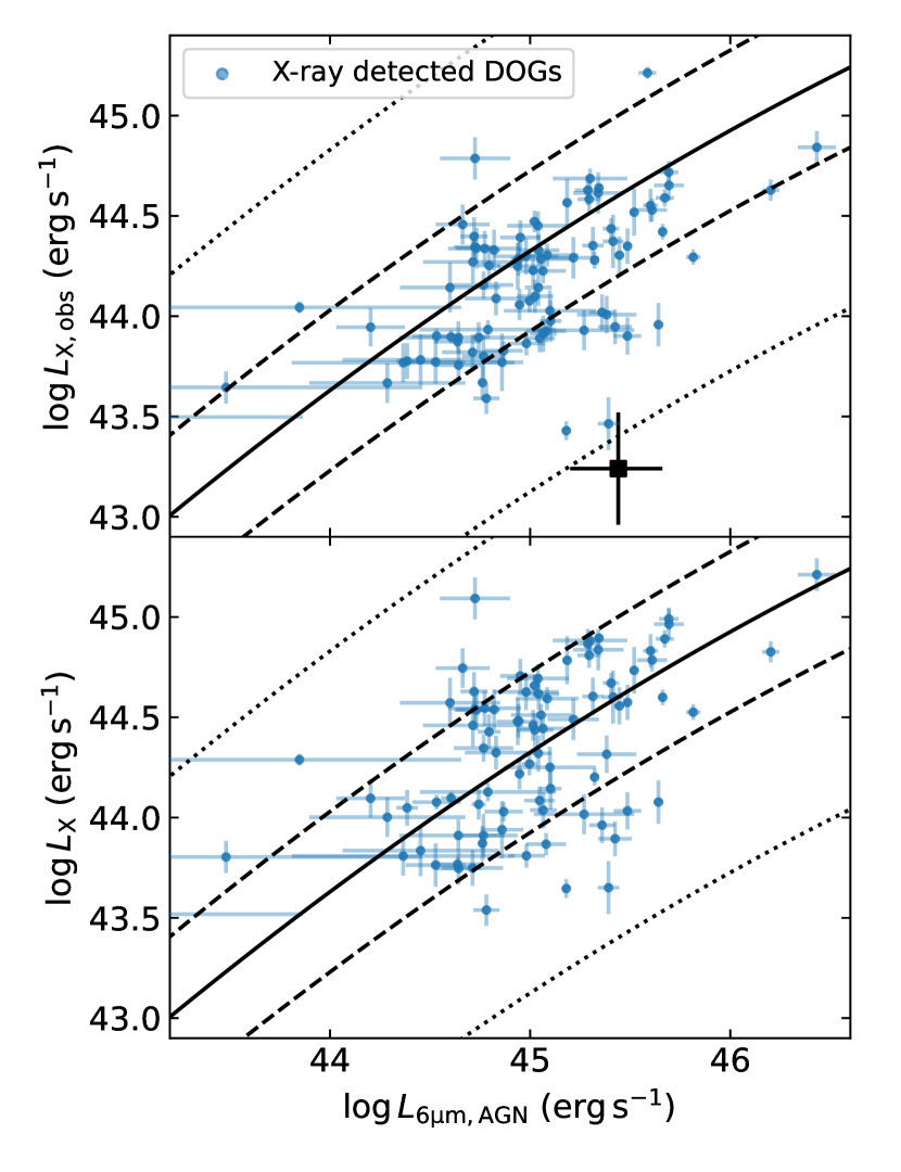
Figure 15: Top panel: the rest-frame $2-10\,\rm keV$ $L_{\mathrm{X,obs}}$ versus $L_{\mathrm{6\mu m,AGN}}$ for the core sample. Bottom Panel: the rest-frame $2-10\,\rm keV$ absorption-corrected $L_{\mathrm{X}}$ versus $L_{\mathrm{6\mu m,AGN}}$ for the core sample. The blue points represent X-ray detected DOGs, and the associated error bars represent $1\sigma$ uncertainties. The black square represents the stacked average $L_{\mathrm{X,obs}}$ versus the median $L_{\mathrm{6\mu m,AGN}}$ for X-ray undetected reliable SED AGNs. The solid line shows the absorption-corrected $L_{\mathrm{X}}-L_{\mathrm{6\mu m,AGN}}$ relation in Stern (2015); the dashed and dotted lines are the $1\sigma$ and $3\sigma$ dispersions of their sample. The results for our full sample are similar.

3.5 Radio Properties

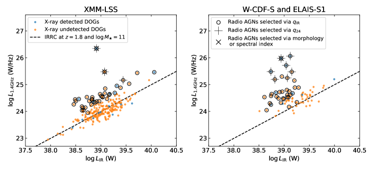
Figure 16: $L_{\mathrm{1.4\,GHz}}$ versus $L_{\mathrm{IR}}$ for our core sample. The left panel shows sources in XMM-LSS, and the right panel shows sources in W-CDF-S and ELAIS-S1. XMM-LSS has much higher radio sensitivity and thus has more radio-detected DOGs. X-ray detected and X-ray undetected DOGs are shown in blue and orange, respectively. The empty circles represent radio AGNs selected via $q_{\mathrm{IR}}$ in Zhang et al. (submitted). The plus signs represent radio AGNs selected via $q_{24}$ in Zhu et al. (2023). The “X”s represent radio AGNs selected via morphology or spectral index in Zhu et al. (2023). The dashed lines represent the IRRC of Delvecchio et al. (2021) at $z=1.8$ and $\log M_{\star}/M_{\sun}=11$ with an additional 0.3 dex offset.

The XMM-SERVS fields are also covered by sensitive radio surveys at $1.4\,\rm GHz$, including the ATLAS in W-CDF-S and ELAIS-S1 (Norris et al., 2006; Hales et al., 2014; Franzen et al., 2015), and a VLA survey and the MIGHTEE survey in XMM-LSS (Heywood et al., 2020, 2022). MIGHTEE covers $3.5\deg^{2}$ in XMM-LSS and reaches a superb $5\sigma$ sensitivity of $28\,\mathrm{\mu Jy}$; the other surveys are relatively shallower ($5\sigma$ sensitivity $\approx 85\,\mathrm{\mu Jy}$) but cover wider areas. These radio data have been extracted and analyzed by Zhu et al. (2023) and matched to our DOGs. There are 745 (20.0%) and 317 (24.4%) DOGs with $1.4\,\rm GHz$ detections in the full and core samples, respectively.

Both SF processes and AGN processes (e.g., jets) can produce radio emission from extragalactic sources. However, SF-related radio emission generally follows a tight correlation with the IR emission, which is known as the IR-radio correlation (IRRC; e.g., Condon, 1992; Tabatabaei et al., 2017; Delvecchio et al., 2017, 2021). To identify radio AGNs, one can look for radio emission that exceeds the levels predicted by the IR emission from SF. Two parameters are often used to identify radio excess: one is the observed $24\,\mu$m-to-1.4 GHz flux ratio (e.g., Appleton et al., 2004): $q_{24}=\log(f_{\mathrm{24\,\rm\mu m}}/f_{\mathrm{1.4\,\rm GHz}})$, where $f_{\mathrm{1.4\,\rm GHz}}$ is the flux density at observed-frame $1.4\,\rm GHz$; the other is the rest-frame FIR-to-radio flux ratio (e.g., Sargent et al., 2010): $q_{\mathrm{IR}}=\log(\frac{L_{\mathrm{IR}}[\mathrm{W}]}{3.75\times 10^{12}[\mathrm{Hz}]})-\log(L_{\mathrm{1.4GHz}}[\mathrm{W/Hz}])$, where $L_{\mathrm{IR}}$ is the rest-frame 8–1000 $\mu$m total luminosity, and $L_{\mathrm{1.4GHz}}$ is the monochromatic luminosity at rest-frame 1.4 GHz. Sources with radio excess (i.e., low $q_{24}$ or low $q_{\mathrm{IR}}$) can be identified as radio AGNs. Zhu et al. (2023) employed the criterion for $q_{24}$ in Appleton et al. (2004) in XMM-SERVS and identified 1763 radio AGNs; Zhang et al. (submitted) employed the $q_{\mathrm{IR}}$ criterion in Delvecchio et al. (2021) and identified 6766 radio AGNs in XMM-SERVS. The $q_{\mathrm{IR}}$ criterion is more complete than the $q_{24}$ criterion, leading to a sample size $\approx 4$ times that of Zhu et al. (2023) while maintaining a satisfactory purity of $\approx 95.2\%$. In fact, the $q_{24}$ criterion may not be very applicable to our DOGs with luminous AGNs since there is significant AGN contamination in the MIR. As we have shown in Section 3.4, most of our AGN candidates are dominated by the AGN component at rest-frame $6\,\mu\rm m$, which approximately corresponds to $12-24\,\mu\rm m$ in the observed-frame. On the other hand, $L_{\mathrm{IR}}$ over rest-frame 8–1000 $\mathrm{\mu m}$ is less affected, where only 31% of DOGs have fractional AGN contributions of $>50\%$. $L_{\mathrm{IR}}$ is also not primarily driven by the $24\,\mathrm{\mu m}$ photometry since approximately half of our DOGs have at least one Herschel FIR band with $\mathrm{SNR}>5$. Note that we do not use the conventional radio-loudness parameter for luminous quasars (e.g., Kellermann et al., 1994) since it assumes that the optical emission is dominated by AGNs, which is not the case for our sources. We also do not rely on the radio module in CIGALE to calculate $q_{\mathrm{IR}}$ because CIGALE only considers the host-galaxy contribution to $q_{\mathrm{IR}}$ and the AGN contribution is controlled by the radio-loudness parameter (Yang et al., 2022), while we compare the total $q_{\mathrm{IR}}$ with the IRRC to identify radio-excess AGNs.

Figure 16 presents $L_{\mathrm{1.4\,\rm GHz}}$ versus $L_{\mathrm{IR}}$ for our core sample. We plot sources in XMM-LSS separately, as MIGHTEE provides a much deeper radio depth than those in the other two fields, which results in more radio-detected DOGs in XMM-LSS (237) than in the other two fields (80). For comparison, we also show the IRRC of Delvecchio et al. (2021), assuming $z=1.8$ and $\log M_{\star}/M_{\sun}=11$, with an additional 0.3 dex offset that accounts for the systematic difference in $L_{\mathrm{IR}}$ following Zhang et al. (submitted). Most DOGs follow a strong correlation between $L_{\mathrm{1.4\,\rm GHz}}$ and $L_{\mathrm{IR}}$, as predicted by the IRRC. We mark radio AGNs selected via $q_{\mathrm{IR}}$ and $q_{24}$, as well as those selected via morphology or spectral index in Zhu et al. (2023), which are generally independent indicators of radio excess. All these radio AGNs show elevated $L_{\mathrm{1.4\,\rm GHz}}$. 39 (34) radio AGNs are identified via $q_{\mathrm{IR}}$ in XMM-LSS (W-CDF-S and ELAIS-S1), constituting 16.3% (42.5%) of the radio-detected DOGs. Fewer radio AGNs are identified via $q_{24}$ (3 in XMM-LSS and 7 in W-CDF-S and ELAIS-S1) and they generally have the strongest radio emission among DOGs. This can be explained by the fact that the AGN component generally is dominant at rest-frame 6 $\mu$m, so sources require much stronger radio emission to be selected via $q_{24}$.

Among the 73 radio AGNs selected via $q_{\mathrm{IR}}$, only 16 of them are identified as reliable SED AGNs. Only one of the three radio AGNs selected by morphology or spectral index is identified as a reliable SED AGN. There are 15 radio AGNs detected in X-rays, and they are all identified as X-ray AGNs. We stack the X-ray images of the 30 X-ray undetected radio AGNs away from known X-ray sources, and we do not obtain detections at $>2\sigma$ significance in any X-ray band. Previous work on the VLA/FIRST $1.4\,\rm GHz$ detected radio-excess DOG J1406+0102 does not show an X-ray detection either (Fukuchi et al., 2023). Despite the relatively small sample size of radio AGNs among DOGs, the AGN selection results based upon radio, SED, and X-rays show minimal overlap. This indicates that radio selection can identify AGNs that can hardly be selected via other methods among DOGs, which aligns with the general results for radio AGN selection in XMM-SERVS (Zhu et al., 2023).

Zhu et al. (2023) also compiled counterparts of their $1.4\,\rm GHz$ radio sources at lower and higher radio frequencies in the three XMM-SERVS fields. The utilized radio surveys include the LOw Frequency ARray (LOFAR; Hale et al., 2019) observations at $144\,\rm MHz$ of XMM-LSS, the Rapid ASKAP Continuum Survey (RACS; McConnell et al., 2020) at $887.5\,\rm MHz$ of all three fields, and the $2.3\,\rm GHz$ ATLAS observations of W-CDF-S and ELAIS-S1 (Zinn et al., 2012). Among our 237 (80) core-sample radio-detected DOGs in XMM-LSS (W-CDF-S and ELAIS-S1), only 9 (7) of them are detected by LOFAR or RACS (RACS or ATLAS $2.3\,\rm GHz$). We further calculate their radio spectral slopes between $1.4\,\rm GHz$ and lower/higher frequencies. Considering their higher detection rates compared to RACS, we use LOFAR measurements in XMM-LSS when possible, and we use ATLAS $2.3\,\rm GHz$ measurements for W-CDF-S and ELAIS-S1 when available. Among the 16 radio-detected DOGs, the median radio spectral slope ($\alpha_{r}$) is –0.65, and only 5 of them are identified as flat-spectrum radio sources (defined as $\alpha_{r}>-0.5$). There is one steep-spectrum radio source ($\alpha_{r}=-0.94$) showing extended double-lobe radio emission, which is consistent with the radio-AGN unification model where steep-spectrum radio sources tend to have lobe-dominated radio morphology (e.g., Tadhunter, 2008; Pyrzas et al., 2015).

4 Discussion

4.1 AGN Fractions

In this subsection, we investigate the fraction of our DOGs hosting accreting SMBHs above a certain accretion-rate threshold ($\lambda_{\mathrm{thres}}$), i.e., the AGN fraction ($f_{\mathrm{AGN}}$). Following Aird et al. (2018), we define specific black-hole accretion rate ($\lambda$) in dimensionless units, such that

$$\lambda=k\,L_{\mathrm{X}}/M_{\star},$$ (5)

where

$$k=\frac{k_{\mathrm{bol}}}{1.3\times 10^{38}\,\mathrm{erg}\,\mathrm{s}^{-1}\times 0.002\,M_{\sun}^{-1}}.$$ (6)

$L_{\mathrm{X}}$ is the absorption-corrected rest-frame $2-10\,\mathrm{keV}$ luminosity, and $k_{\mathrm{bol}}$ is the bolometric correction factor (we adopt $k_{\mathrm{bol}}=25$ in this paper following Aird et al., 2018). We choose the additional factor $k$ so that $\lambda$ is approximately the Eddington ratio ($\lambda_{\mathrm{Edd}}$). We further assume a constant $\lambda$ at its typical value $\lambda_{0}$ for sources accreting above a certain threshold ($\lambda_{0}>\lambda_{\mathrm{thres}}$; i.e., $f_{\mathrm{AGN}}$ of our sources accrete at $\lambda_{0}$, and the others accrete below $\lambda_{\mathrm{thres}}$). Aird et al. (2018) have shown that for AGNs accreting at $\lambda>0.01$, $\langle\lambda\rangle\approx 0.1-1$, where $\langle\lambda\rangle$ is the average specific accretion rate. In fact, the similarity between $\lambda$ and $\lambda_{\mathrm{Edd}}$ already provides a reasonable range of typical $\lambda$, as we would expect most sources are at sub-Eddington levels.

Considering the contribution from all sources, Equation 5 becomes

$$f_{\mathrm{AGN}}=k\,\lambda_{0}^{-1}\,\sum L_{\mathrm{X}}/\sum M_{\star},$$ (7)

where the summations run over all sources in the sample. A simple, intuitive physical interpretation of Equation 7 is that $\lambda_{0}$ and $f_{\mathrm{AGN}}$ are degenerate: for a given total intrinsic X-ray luminosity from all sources, the more powerful the central engines are, the lower is the required AGN fraction.

The total intrinsic X-ray luminosity is contributed by both the X-ray detected sources and the undetected ones, and our $f_{\mathrm{AGN}}$ have considered both. We use the absorption-corrected $L_{\mathrm{X}}$ in Sections 3.2 and 3.3 for X-ray detected and X-ray undetected DOGs, respectively. Assuming a constant $\lambda_{0}=0.1$, we obtain $f_{\mathrm{AGN}}=15\%$ for our full sample; if $\lambda_{0}=1$, $f_{\mathrm{AGN}}=1.5\%$. As for the core sample, when $\lambda_{0}=0.1-1$, $f_{\mathrm{AGN}}=20-2.0\%$. These values are generally consistent with the typical AGN fraction of $10-20\%$ at $z\approx 1.8$ and $\log M_{\star}\approx 11$ (i.e., our median $z$ and $\log M_{\star}$, Xue et al., 2010; Aird et al., 2018; Zou et al., 2024). This indicates that DOGs do not appear to host a distinctively higher fraction of AGNs. The AGN fraction for DOGs is also similar to that of $17^{+16}_{-6}\%$ for SMGs at $z\approx 2-3$ (Wang et al., 2013) which are also strongly star-forming and dusty (e.g., Alexander et al., 2005). However, Hot DOGs, a more extreme subset of HyLIRGs with extreme MIR colors, have been found to host stronger AGN activity than reddened quasars (Vito et al., 2018). They are thought to be at the peak of SMBH accretion when the feedback has not yet swept away the surrounding gas and dust in the merger-driven coevolution framework. Our results show that DOGs, in general, do not present significantly different SMBH accretion compared with AGNs among a matched typical galaxy population, at least for those selected via the criteria of Dey et al. (2008).

4.2 Comparison between X-ray Detected DOGs and non-DOG X-ray AGNs

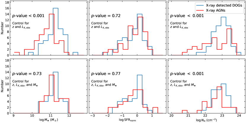
Figure 17: Example distributions of $M_{\star}$ (left column), $\mathrm{SFR_{norm}}$ (middle column), and $N_{\mathrm{H}}$ (right column) for our X-ray detected DOGs in the core sample (blue) compared with those for non-DOG X-ray AGNs (red). We control for $z$ and $L_{\mathrm{X,obs}}$ in the top row, and we control for $z$, $L_{\mathrm{X,obs}}$, and $M_{\star}$ in the bottom row. When we only control for $z$ and $L_{\mathrm{X,obs}}$, $M_{\star}$ and $N_{\mathrm{H}}$ both show distinct differences between X-ray detected DOGs and X-ray AGNs, while the difference in $\mathrm{SFR_{norm}}$ is not significant. After we further control for $M_{\star}$, the difference in $\mathrm{SFR_{norm}}$ remains insignificant, and the difference in $N_{\mathrm{H}}$ remains significant. Note that further controlling for $M_{\star}$ makes building consistent comparison samples more difficult, which results in fewer sources in the bottom panels.

Table 6: Differences between X-ray detected DOGs and non-DOG X-ray AGNs after 1000 trials.

Subsample	Controlled parameters	$p$-values for $M_{\star}$	$p$-values for $\mathrm{SFR_{norm}}$	$p$-values for $N_{\mathrm{H}}$	$\Delta\overline{\log M_{\star}}$	$\Delta\overline{\log\mathrm{SFR_{norm}}}$	$\Delta\overline{\log N_{\mathrm{H}}}$	Number of sources compared
(1)	(2)	(3)	(4)	(5)	(6)	(7)	(8)	(9)
Full	$z$ and $L_{\mathrm{X,obs}}$	$<0.001$	$0.8_{-0.3}^{+0.1}$	$<0.001$	$0.38_{-0.07}^{+0.04}$	$0.05_{-0.07}^{+0.06}$	$0.40_{-0.04}^{+0.09}$	87
	$z$, $L_{\mathrm{X,obs}}$, and $M_{\star}$	$>0.97$	$0.5_{-0.3}^{+0.3}$	$<0.001$	$-0.01_{-0.02}^{+0.03}$	$0.18_{-0.08}^{+0.09}$	$0.61_{-0.23}^{+0.15}$	70
Core	$z$ and $L_{\mathrm{X,obs}}$	$<0.001$	$0.7_{-0.3}^{+0.2}$	$<0.001$	$0.35_{-0.06}^{+0.07}$	$-0.01_{-0.07}^{+0.10}$	$0.52_{-0.20}^{+0.20}$	51
	$z$, $L_{\mathrm{X,obs}}$, and $M_{\star}$	$>0.94$	$0.4_{-0.2}^{+0.3}$	$<0.001$	$0.06_{-0.04}^{+0.05}$	$0.20_{-0.09}^{+0.10}$	$0.44_{-0.12}^{+0.20}$	39

Note. — Column (1): our full sample and core sample. Column (2): parameters controlled when making the comparison X-ray AGN sample. Columns (3)–(5): median $p$-values and their associated 68% confidence intervals when performing AD tests on $M_{\star}$, $\mathrm{SFR_{norm}}$, and $N_{\mathrm{H}}$ between X-ray detected DOGs and non-DOG X-ray AGNs. If the median $p$-values are less than 0.001 (greater than 0.97), we only show “$<0.001$” (“$>0.97$”). Columns (6)–(7): differences in the median values of $\log M_{\star}$, $\log\mathrm{SFR_{norm}}$, and $\log N_{\mathrm{H}}$. We show the median differences and the associated 68% confidence intervals. Column (8): Number of sources in each comparison sample.

Under the merger-driven galaxy-SMBH coevolution framework, DOGs also represent the peak phase of SF before the fast SMBH growth. In this subsection, we discuss how X-ray detected DOGs differ from X-ray AGNs not selected as DOGs. We focus on their host-galaxy properties and X-ray obscuration. All our X-ray detected DOGs are identified as AGN candidates using the SED-based method of Zou et al. (2022), and they are all identified as X-ray AGNs in Chen et al. (2018) and Ni et al. (2021). Together with the high $L_{\mathrm{X,obs}}$ shown in Figure 7, the results indicate good classification purity.

Since host-galaxy properties and X-ray obscuration correlate with $z$ and $L_{\mathrm{X}}$, we need to control for these factors. For instance, high-luminosity AGNs generally have enhanced SFRs compared to star-forming galaxies at similar $z$ and $M_{\star}$ (e.g., Mountrichas et al., 2024). Also, X-ray obscuration in AGNs shows significant cosmic evolution, increasing strongly from $z\approx 0$ to $z\approx 2$ (e.g., Buchner et al., 2015; Georgakakis et al., 2017; Liu et al., 2017); at a given redshift, AGNs tend to have less X-ray obscuration at higher luminosities (e.g., Merloni et al., 2014; Liu et al., 2017). We consider X-ray detected sources within $z=0-4$ and $\log L_{\mathrm{X,obs}}=43-46$, where 87 sources in the full sample and 51 sources in the core sample are included. We divide the $z-\log L_{\mathrm{X,obs}}$ plane into a grid with $\Delta z=0.2$ and $\Delta\log L_{\mathrm{X,obs}}=0.4\,\rm dex$. In each cell, we denote the number of X-ray detected DOGs in field $S$ ($S=1,2,\text{ or }3$, denoting one of the three fields covered by XMM-SERVS) as $N_{S,1}$, and the number of non-DOG X-ray AGNs as $N_{S,2}$. We randomly select $\min\{N_{S,1},N_{S,2}\}$ X-ray detected DOGs and the same number of non-DOG X-ray AGNs in field $S$. We then combine all the selected sources across the three fields. The above steps conserve the number of sources from different fields in our comparison sample to mitigate any possible effects across different fields. After repeating the above steps in each cell and each field, we can construct new X-ray detected DOG and non-DOG X-ray AGN samples with similar distributions of $z$ and $L_{\mathrm{X,obs}}$. Since there are many more general X-ray AGNs than X-ray detected DOGs, in most grids the number of selected objects is controlled by the number of X-ray detected DOGs. For a typical example of those randomly chosen sources based upon our core sample (51 X-ray detected DOGs and 51 non-DOG X-ray AGNs), we use a two-sample AD test to examine the consistency of $z$ and $L_{\mathrm{X,obs}}$, and the $p$-values of $z$ and $L_{\mathrm{X,obs}}$ are 0.97 and 0.78, respectively, indicating that these two parameters have been controlled acceptably.

In the top row of Figure 17, we compare the distributions of $M_{\star}$, $\mathrm{SFR_{norm}}$, and $N_{\mathrm{H}}$ for a typical example of randomly chosen X-ray DOGs and X-ray AGNs using the above procedure. We do not exclude “unsafe” sources (i.e., whose MS cannot be reliably obtained) from the comparison of $\mathrm{SFR_{norm}}$ because the $\mathrm{SFR_{norm}}$ distribution is not significantly affected by them as shown in Section 3.1. We find that X-ray detected DOGs generally have higher $M_{\star}$ and $N_{\mathrm{H}}$ than typical X-ray AGNs, while the SFR does not have significant differences. We further run AD tests on these distributions, finding that the difference is statistically significant for $M_{\star}$ and $N_{\mathrm{H}}$ with both $p$-values $<0.001$. As for $\mathrm{SFR_{norm}}$, the difference is insignificant with a $p$-value of 0.72. The result that X-ray detected DOGs appear to have higher obscuration levels than typical X-ray AGNs could be at least partly caused by their higher $M_{\star}$. There have been findings of a positive correlation between $M_{\star}$ and X-ray obscuration level (e.g., Lanzuisi et al., 2017). It is also possible that galaxy-scale gas and dust can contribute to the obscuration of AGNs (Buchner & Bauer, 2017; Gilli et al., 2022), and the $N_{\mathrm{H}}$ of galaxy-scale gas also follows a positive correlation with $M_{\star}$ (e.g., Buchner et al., 2017). To eliminate the impact of $M_{\star}$ on $N_{\mathrm{H}}$, we further control for $M_{\star}$  in addition to $z$ and $L_{\mathrm{X,obs}}$ and test if the difference in $N_{\mathrm{H}}$ remains. We show the new results for $M_{\star}$, $\mathrm{SFR_{norm}}$, and $N_{\mathrm{H}}$ in the bottom row of Figure 17. As expected, the difference in $M_{\star}$ is no longer significant with $p$-$\mathrm{value}=0.73$. However, $N_{\mathrm{H}}$ is still significantly different between X-ray detected DOGs and X-ray AGNs with $p$-$\mathrm{value}<0.001$. The difference in $\mathrm{SFR_{norm}}$ remains insignificant with $p$-$\mathrm{value}=0.77$.

We further use a Monte Carlo method to check the robustness of our statistical results. We repeat the above test 1000 times for both the full and core samples, and each time the randomly chosen samples are different. We also calculate the difference in the median values of $\log M_{\star}$ ($\Delta\overline{\log M_{\star}}$), $\log\mathrm{SFR_{norm}}$ ($\Delta\overline{\log\mathrm{SFR_{norm}}}$), and $\log N_{\mathrm{H}}$ ($\Delta\overline{\log N_{\mathrm{H}}}$) between our X-ray detected DOGs and matched X-ray AGNs. We show the median $p$-values and the median differences and their associated 68% confidence intervals in Table 6. Overall, the results show that X-ray detected DOGs generally have higher $M_{\star}$ and higher $N_{\mathrm{H}}$ than typical X-ray AGNs across different samples when $z$ and $L_{\mathrm{X,obs}}$ are controlled. Also, X-ray detected DOGs do not appear to be more actively star-forming than typical X-ray AGNs. After we further control for $M_{\star}$, the difference in $N_{\mathrm{H}}$ is still significant; X-ray detected DOGs appear to have slightly higher $\mathrm{SFR_{norm}}$, but the difference is still insignificant given the large $p$-values. Note that we do not apply any selection correction to obtain the intrinsic $N_{\mathrm{H}}$ distribution; rather, we present the observed distributions and compare two sub-populations within the same parent sample (i.e., X-ray sources in XMM-SERVS).

Apart from $M_{\star}$, $\mathrm{SFR_{norm}}$, and $N_{\mathrm{H}}$, we further examine the IR flux densities of DOGs. We find that the reliable SED AGN fraction among our core sample increases significantly with $f_{\mathrm{24\mathrm{\mu m}}}$, which is consistent with previous works finding that the fraction of PL sources among DOGs increases with IR flux density (e.g., Melbourne et al., 2012; Toba et al., 2015). The results are similar for our full sample. We then compare $f_{\mathrm{24\mathrm{\mu m}}}$ between matched X-ray detected DOGs and non-DOG X-ray AGNs. These samples are constructed following the same procedure outlined in this Section. We find that $f_{\mathrm{24\mathrm{\mu m}}}$ for our X-ray detected DOGs is significantly higher than for matched X-ray AGNs. This is expected, as our DOGs are constructed to have $f_{\mathrm{24\mathrm{\mu m}}}>0.3\,\mathrm{mJy}$, while many matched typical X-ray AGNs have $f_{\mathrm{24\mathrm{\mu m}}}$ below this threshold.

The similar $\mathrm{SFR_{norm}}$ and higher $M_{\star}$ for X-ray detected DOGs compared with typical X-ray AGNs cast doubt on the relevance of the merger-driven coevolution framework for DOGs, which postulates that DOGs should be on the peak phase of SF (e.g., Hopkins et al., 2006, 2008; Narayanan et al., 2010; Yutani et al., 2022). We argue that a more natural interpretation of our results is that X-ray detected DOGs can be regarded as analogs to extreme type 2 AGNs. Type 2 AGNs show strong dust emission and are heavily obscured in the optical bands, which contributes to the selection of X-ray detected DOGs. Traditionally, AGNs can be classified into type 1 and type 2 objects, where type 1 AGNs show broad optical emission lines (specifically, the Balmer lines), while type 2 AGNs only have narrow lines. Both DOGs and type 2 AGNs are obscured in the optical band, although broad-line DOGs (e.g., Toba et al., 2017; Zou et al., 2020) and blue-excess IR-bright DOGs (BluDOGs; e.g., Noboriguchi et al., 2019, 2022) are also observed. These may be attributed to strong starburst or leaked UV emission from the central AGN. These sources may be explained by leaked emission via reflection or from partially covered Broad-Line Regions (BLRs), especially in cases where the AGN component is strong (e.g., Assef et al., 2016). Recent studies have shown that type 2 AGNs tend to have higher $M_{\star}$ than type 1 AGNs, but both types have similar SFR distributions (e.g., Zou et al., 2019; Mountrichas et al., 2021). The higher $M_{\star}$ for type 2 AGNs can be explained if galaxy-wide gas and dust contribute to the obscuration of AGNs, and thus type 2 AGNs tend to reside in more massive galaxies because more massive galaxies have more dust (e.g., Whitaker et al., 2017). These results are consistent with our findings if X-ray detected DOGs are considered extreme type 2 AGNs. In addition, observations have shown that PL DOGs tend to have slightly higher $M_{\star}$ than Bump DOGs (e.g., Bussmann et al., 2012). As we confirmed in Section 2.3, PL DOGs are more AGN-dominated, and their higher $M_{\star}$ can be explained if PL DOGs are more similar to type 2 AGNs than Bump DOGs due to their higher AGN purity. Since DOGs are more obscured in the optical bands due to galaxy-wide dust, the higher $M_{\star}$ values of our X-ray detected DOGs also indicate that the galaxy-wide dust is indeed connected to $M_{\star}$. However, the consistently higher $N_{\mathrm{H}}$ for X-ray detected DOGs even when we control for $M_{\star}$ also shows that their AGN obscuration is not solely determined by the galaxy-wide obscuration and should be primarily contributed by the higher nuclear obscuration among X-ray detected DOGs.

Our results are in agreement with those in Li et al. (2020) who found that secular processes, instead of mergers, are most probable to trigger X-ray-selected, heavily obscured AGNs that show less-extreme optical-IR colors. However, we cannot simply rule out the relevance of mergers. For our X-ray detected DOGs, the similar $\mathrm{SFR_{norm}}$ compared with matched typical X-ray AGNs could be explained in the merger-driven SMBH-galaxy coevolution framework if X-ray detected DOGs are in a slightly later evolutionary phase than X-ray undetected ones, in which the star-formation has been reduced a bit due to feedback. Observational constraints on the host morphology and/or stellar and gas dynamics can provide more direct evidence for/against the relevance of mergers for DOGs. The relevance may also differ among DOGs with different extreme levels, and further division of DOGs into different subsets may help us understand such differences. For instance, Hot DOGs show larger $N_{\mathrm{H}}$ than those derived for type 1 quasars with similar luminosities (Vito et al., 2018), consistent with a post-merger stage; high-$\lambda_{\mathrm{Edd}}$ DOGs are found to be in similar evolutionary stages as Hot DOGs, and both SMBH accretion and host-galaxy SF are reaching the highest level (Zou et al., 2020).

5 Summary and Future Work

In this work, we select 3738 DOGs in XMM-SERVS as a full sample using the same selection criteria as Dey et al. (2008), among which 174 are detected in X-rays. To ensure reliable redshifts, we further select 1309 DOGs with spec-$z$s or reliable photo-$z$s as a core sample, among which 88 are detected in X-rays. The large survey volume and deep multiwavelength coverage of XMM-SERVS provide high-quality characterization of DOGs and make our sample size substantially exceed those of previous comparable studies. We analyze DOG properties based upon SED-fitting, X-ray, and radio observations. Critically, we assess if DOGs represent the key evolutionary phase in the merger-driven galaxy-SMBH coevolution framework. The main results are the following:

1. Our core sources are at $z=1.63-1.93$ ($25-75$% quantiles) with a median $L_{\mathrm{bol}}=10^{12.4}\,L_{\sun}$. The median $L_{\mathrm{bol}}$ is much higher than that for typical X-ray AGNs but is much lower than for the most-extreme Hot DOGs. There are $\approx 10\%$ of DOGs identified as reliable SED AGNs, and we confirm that the phenomenologically defined PL DOGs indeed preferentially host AGNs. The X-ray detected DOGs are generally luminous (median $L_{\mathrm{X,obs}}=10^{44.3}\,\mathrm{erg}\,\mathrm{s}^{-1}$). The results for our full sample are similar. See Sections 2.3 and 2.4.

2. Our DOGs are massive with median $\log M_{\star}\approx 11$. X-ray detected DOGs have slightly higher $M_{\star}$ than X-ray undetected DOGs, which can be explained by the connection between SMBH accretion and $M_{\star}$. As for $\mathrm{SFR_{norm}}$, X-ray undetected DOGs generally lie on or above the star-formation MS relation calibrated in XMM-SERVS, reaching up to starburst galaxies. In contrast, a significant fraction of X-ray detected DOGs lie below the MS. See Section 3.1.

3. We perform X-ray stacking analyses of X-ray undetected DOGs and find significant average detections in all three bands for both the full and core samples. The median average $L_{\mathrm{X,obs}}$ is $(4.3\pm 1.7)\times 10^{42}\,\mathrm{erg}\,\mathrm{s}^{-1}$ for our core sample. Stacking several subsets also reveals that the total accretion power of X-ray undetected DOGs is primarily contributed by AGN candidates identified via their SEDs. See Section 3.3.

4. We find about half of our X-ray detected DOGs are identified as heavily obscured ($N_{\mathrm{H}}>10^{23}\,\mathrm{cm}^{-2}$) AGNs based upon their HRs. X-ray stacking also indicates that X-ray undetected DOGs identified as AGN candidates have $N_{\mathrm{H}}\gtrsim 10^{23}\,\mathrm{cm}^{-2}$ on average. The results on $L_{\mathrm{X,obs}}$ versus $L_{\mathrm{6\mu m,AGN}}$ confirm their heavily obscured nature. Overall, X-ray undetected DOGs identified as reliable SED AGNs are more obscured in X-rays than X-ray detected ones, and some likely reach CT levels. See Sections 3.2 and 3.4.

5. Most radio-detected DOGs show a strong correlation between $L_{\mathrm{1.4\,\rm GHz}}$ and $L_{\mathrm{IR}}$, and DOGs selected as radio AGNs show much elevated $L_{\mathrm{1.4\,\rm GHz}}$. We find that radio selection can select AGNs among DOGs that can hardly be selected via other methods, consistent with the results on general radio AGN selection in, e.g., Zhu et al. (2023). See Section 3.5.

6. Combining the individual fluxes of X-ray detected DOGs and the stacked X-ray images for X-ray undetected DOGs, we estimate the AGN fractions to be 1.5–15% and 2.0–20% for our DOG full sample and core sample, respectively, considering a constant $\lambda_{0}=1-0.1$. The values are consistent with the AGN fraction of 10–20% for typical galaxy populations at $z\approx 2$ with $\log M_{\star}\approx 11$, indicating that DOGs do not present significantly different SMBH accretion compared with AGNs in typical galaxy populations. See Section 4.1.

7. We control for $z$ and $L_{\mathrm{X,obs}}$ and find that X-ray detected DOGs have higher $M_{\star}$ and $N_{\mathrm{H}}$ than non-DOG X-ray AGNs in XMM-SERVS, while their $\mathrm{SFR_{norm}}$ distributions are similar even after we further control for $M_{\star}$. The results challenge the relevance of the merger-driven galaxy-SMBH coevolution framework for X-ray detected DOGs and suggest that they may be analogs to extreme type 2 AGNs that show similar behaviors. See Section 4.2.

This work presents the largest sample of DOGs in sensitive multiwavelength surveys. Critical advances for this sample will be made once future deep spectroscopic and photometric data from, e.g., MOONS, PFS, 4MOST WAVES, LSST, Euclid, and LMT TolTEC are gathered in XMM-SERVS. In particular, deep spectroscopic surveys can not only provide a larger sample with better completeness of reliable redshifts, but also provide rich diagnostic information from spectroscopy, which can help better characterize the sample and even break it down into physically relevant subsets (e.g., high-$\lambda_{\mathrm{Edd}}$ DOGs; Zou et al., 2020). LMT TolTEC will provide sensitive submillimeter data, which will help better characterize the star-formation and dust properties of these DOGs. Spatially resolved imaging and/or spectroscopy from JWST for a representative subset of DOGs can probe the host morphology and dynamics, providing a direct test of the relevance of mergers for DOGs.

Appendix A The Reliability of $M_{\star}$ and SFR Measurements

In Section 3.1, we measured $M_{\star}$ and SFR of our DOGs via SED-fitting. In this Appendix, we further check the reliability of our measurements. For sources hosting strong AGN components, the rest-frame NIR SED may be dominated by the AGN component, making $M_{\star}$ usually less reliable. We denote $M_{\star}^{\mathrm{gal}}$ as the $M_{\star}$ fitted using normal-galaxy templates (i.e., without the AGN component) in Zou et al. (2022). Since the contribution from the AGN component is then assigned to the galaxy component, $M_{\star}^{\mathrm{gal}}$ can be considered a soft upper limit for the true $M_{\star}$. We use our samples in W-CDF-S as an illustration. We plot the difference in $\log M_{\star}$ ($\Delta\log M_{\star}$) in the top-left panel of Figure 18. The median $\Delta\log M_{\star}=0.08$ and $\sigma_{\mathrm{NMAD}}=0.17$ for our core sample. The results are similar for the other two fields, and indicate that the AGN component does not impact our measurements of $M_{\star}$ significantly. We also plot $\Delta\log M_{\star}$ versus redshift in the bottom-left panel. The results show that $\Delta\log M_{\star}$ is not redshift dependent.

The inclusion of FIR photometry helps accurately measure SFR. About 55% of our sources have $250\,\mathrm{\mu m}$ Herschel SPIRE photometry with $\mathrm{SNR}>5$, which is much higher than the typical fraction in general galaxy samples in XMM-SERVS, and we expect our SFR measurements to be reliable for these sources. However, we still test if the measurements for the rest of the sources are reliable. We exclude the FIR photometry for sources in W-CDF-S and measure their SFRs using the same method as in Zou et al. (2022), and we show the difference in SFR ($\Delta\log\mathrm{SFR}$) in the top-right panel of Figure 18. Visually, there is a weak trend such that $\Delta\log\mathrm{SFR}$ slightly increases toward higher SFR. However, the small median $\Delta\log\mathrm{SFR}$ of 0.02 and $\sigma_{\mathrm{NMAD}}$ of 0.26 for our core sample are similar to or even better than the typical comparison results for XMM-SERVS AGNs in general (Table 7 and Figure 29 of Zou et al., 2022). The results are similar for the other two fields. These indicate that the SFR measurements are not significantly biased for sources without high-quality FIR photometry. We also show $\Delta\log\mathrm{SFR}$ versus redshift in the bottom-right panel. The results show that $\Delta\log\mathrm{SFR}$ does not evolve with redshift.

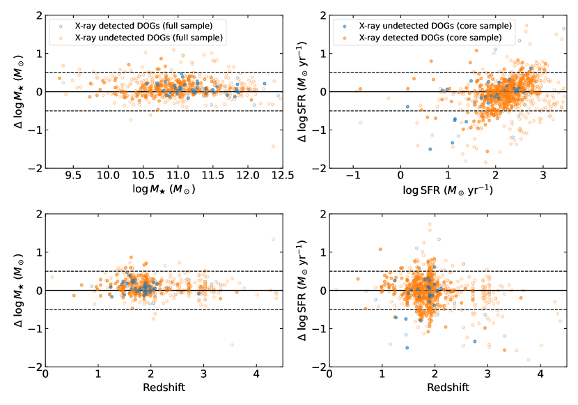
Figure 18: Top-left panel: Comparison between $M_{\star}^{\mathrm{gal}}$ and the adopted AGN-template-based $M_{\star}$ values ($\Delta\log M_{\star}=\log M_{\star}^{\mathrm{gal}}-\log M_{\star}$) for sources with preferred AGN models in W-CDF-S. Bottom-left panel: $\Delta\log M_{\star}$ versus redshift. Top-right panel: Comparison between SFR measurements with and without FIR data in W-CDF-S. Bottom-right panel: $\Delta\log\mathrm{SFR}$ versus redshifts. The full and core samples are shown with empty and filled circles, respectively. X-ray detected and X-ray undetected DOGs are shown in blue and orange, respectively. The differences are generally within 0.5 dex and do not evolve with redshift. The median differences and $\sigma_{\mathrm{NMAD}}$ are small, indicating that our $M_{\star}$ and SFR measurements do not have significant biases.

Appendix B Selection of lower-luminosity Hot DOG Candidates

In Section 2, we presented the selection of DOGs and showed that, as expected, they generally have lower $L_{\mathrm{bol}}$ than the most extreme Hot DOGs with $L_{\mathrm{bol}}>10^{14}\,L_{\sun}$. In this Appendix, we further describe how we select lower-luminosity analogs to those extreme Hot DOGs using the best-fit SED model and selection criteria similar to those in Eisenhardt et al. (2012). The adopted selection criteria in Eisenhardt et al. (2012) are $\mathrm{W1}>17.4$, and either (1) $\mathrm{W4}<7.7$ and $\mathrm{W2}-\mathrm{W4}>8.2$ or (2) $\mathrm{W3}<10.6$ and $\mathrm{W2-W3}>5.3$. Such criteria select luminous ($L_{\mathrm{bol}}>10^{13}\,L_{\sun}$, some even exceed $10^{14}\,L_{\sun}$; Tsai et al., 2015; Li et al., 2024) and rare ($\approx 1$ per 40 $\deg^{2}$) Hot DOGs that are characterized by hot dust temperatures and extreme MIR colors.

Our SEDs fits do not directly provide dust temperature, and thus we select lower-luminosity Hot DOG candidates among our DOG full sample using slightly modified color criteria compared to Eisenhardt et al. (2012): (1) $\mathrm{W1}-\mathrm{W4}>9.7$ and $\mathrm{W2}-\mathrm{W4}>8.2$ or (2) $\mathrm{W1}-\mathrm{W3}>6.8$ and $\mathrm{W2-W3}>5.3$, i.e., we lift the magnitude cuts on W1 and W3/W4 in Eisenhardt et al. (2012) and convert them to color cuts. This modification allows the selection of sources with lower luminosity but with similarly extreme MIR colors. The synthetic WISE photometry in W1–W4 is calculated from the best-fit SEDs, where we calculate the expected WISE flux in W1–W4 by convolving the best-fit SED with the WISE filter response. The flux is then converted to WISE magnitude using the zero-point values in Wright et al. (2010). We have checked that our SED-based WISE magnitude is generally consistent with the AllWISE catalog (Cutri et al., 2021) for sources that are detected in the corresponding WISE band.

We end up with 62 sources out of 3738 DOGs in the full sample selected as lower-luminosity Hot DOG candidates using our modified selection criteria. These candidates are marked in Table 1. Among these candidates, 26 are identified as reliable SED AGNs. The median $L_{\mathrm{bol}}$ of the 62 candidates and the 26 reliable SED AGNs are $10^{12.5}\,L_{\sun}$ and $10^{12.8}\,L_{\sun}$, both of which are much lower than the typical $L_{\mathrm{bol}}$ of $\approx 10^{13}-10^{14}\,L_{\sun}$ for Hot DOGs selected via “W1W2-dropout”. The rest-frame median SEDs for all our Hot DOG candidates and those selected as reliable SED AGNs are shown in Figure 19. For comparison, we also plot the median SED for DOGs that are AGN candidates but are not selected as lower-luminosity Hot DOG candidates, the median SED for Hot DOGs in Fan et al. (2016), and the median SED for high-redshift obscured AGNs in Yang et al. (2023), all of which are normalized at rest-frame 3.6 $\mathrm{\mu m}$. The median SED for our lower-luminosity Hot DOG candidates is similar to that for Hot DOGs in Fan et al. (2016) in the MIR at rest-frame $\lesssim 15\mathrm{\mu m}$. This wavelength range fully covers the WISE bands assuming the median $z\approx 1.8$ of our DOGs. Our Hot DOG candidates show much redder MIR colors than those that are not selected, indicating their relatively stronger hot-dust emission. At longer wavelengths that the WISE bands do not cover, our Hot DOG candidates generally show similar FIR SEDs compared with DOGs that are not selected as Hot DOG candidates. However, Hot DOG candidates selected as reliable SED AGNs still have similar FIR SEDs compared with Hot DOGs in Fan et al. (2016). This is due to the fact that those Hot DOG candidates selected as reliable SED AGNs are more similar to Hot DOGs selected via “W1W2-dropout”, which have higher $L_{\mathrm{bol}}$ and a stronger AGN component in the MIR. These results indicate our criteria indeed select candidates for lower-luminosity version of Hot DOGs. We have also tried the selection criteria in Section 2 of Ricci et al. (2017) for low-redshift Hot DOG candidates. Their criteria are similar to ours except that they have an additional requirement of $\mathrm{W1}<17.4$ to preferentially select bright low-redshift Hot DOGs. We do not find any such low-redshift Hot DOG candidates among our full sample DOGs.

One of our selected Hot DOG candidates is detected in X-rays (XID: WCDFS0530) at $z=1.79$. XMM-Newton observed this source two times, and the total cleaned exposure time is 49.9 ks. It is only marginally detected in the FB, with 76 net counts in total from all three EPIC cameras (Ni et al., 2021). We reduce the observations and extract the spectra using the XMM-Newton Science Analysis System (SAS; v21.0). We use XSPEC (Arnaud, 1996) v12.12.1 to jointly fit all individual X-ray spectra, in which the C-statistic is adopted. We limit our spectral fitting to 0.5–1.4 $\mathrm{keV}$ and 1.6–7.5 $\mathrm{keV}$ due to the high background above $7.8\,\mathrm{keV}$ and the Al K$\alpha$ instrumental background lines at $\approx 1.5\,\mathrm{keV}$. We fit the spectra with a simple power-law with Galactic absorption. The best-fit effective power-law photon index is $\Gamma_{\mathrm{eff}}=0.9_{-0.8}^{+0.9}$, and the best-fit observed-frame 2–10 $\mathrm{keV}$ flux is $5_{-5}^{+10}\times 10^{-15}\,\mathrm{erg}\,\mathrm{cm}^{-2}\,\mathrm{s}^{-1}$. Assuming $\Gamma_{\mathrm{eff}}$ at its best-fit value, its best-fit rest-frame 2–10 $\mathrm{keV}$ $L_{\mathrm{X,obs}}$ is $4_{-4}^{+8}\times 10^{43}\,\mathrm{erg}\,\mathrm{s}^{-1}$. The $L_{\mathrm{6\mu m,AGN}}$ of this source is $1.3\times 10^{46}\,\mathrm{erg}\,\mathrm{s}^{-1}$, which places this source $\approx 3\sigma$ below the Stern (2015) relation in the $L_{\mathrm{X,obs}}-L_{\mathrm{6\mu m,AGN}}$ plane (see Figure 15). The hard best-fit $\Gamma_{\mathrm{eff}}$ and low $L_{\mathrm{X,obs}}/L_{\mathrm{6\mu m,AGN}}$ both indicate the lower-luminosity Hot DOG candidate WCDFS0530 is heavily obscured, consistent with the X-ray study on Hot DOGs in Vito et al. (2018).

We also stack the X-ray images for all our X-ray undetected Hot DOG candidates and those selected as reliable SED AGNs (following Section 3.3, stacked sources are away from known X-ray sources), but none of the X-ray bands shows detections at $>2\sigma$ for both samples.

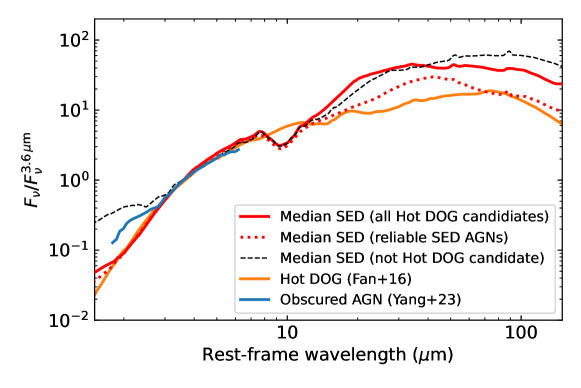
Figure 19: Comparison between different types of median SEDs (normalized at rest-frame 3.6 $\mathrm{\mu m}$). The red solid and dotted curves represent all our lower-luminosity Hot DOG candidates, and those selected as reliable SED AGNs, respectively. The black dashed curve represents DOGs that are not selected as lower-luminosity Hot DOG candidates. The orange and blue solid curves represent Hot DOGs (Fan et al., 2016) and obscured AGNs (Yang et al., 2023).

References

- Abbott et al. (2021) Abbott, T. M. C., Adamów, M., Aguena, M., et al. 2021, ApJS, 255, 20, doi: 10.3847/1538-4365/ac00b3
- Abdurro’uf et al. (2022) Abdurro’uf, Accetta, K., Aerts, C., et al. 2022, ApJS, 259, 35, doi: 10.3847/1538-4365/ac4414
- Aihara et al. (2018) Aihara, H., Armstrong, R., Bickerton, S., et al. 2018, PASJ, 70, S8, doi: 10.1093/pasj/psx081
- Aird et al. (2018) Aird, J., Coil, A. L., & Georgakakis, A. 2018, MNRAS, 474, 1225, doi: 10.1093/mnras/stx2700
- Alexander et al. (2005) Alexander, D. M., Bauer, F. E., Chapman, S. C., et al. 2005, ApJ, 632, 736, doi: 10.1086/444342
- Appleton et al. (2004) Appleton, P. N., Fadda, D. T., Marleau, F. R., et al. 2004, ApJS, 154, 147, doi: 10.1086/422425
- Arnaud (1996) Arnaud, K. A. 1996, in Astronomical Society of the Pacific Conference Series, Vol. 101, Astronomical Data Analysis Software and Systems V, ed. G. H. Jacoby & J. Barnes, 17
- Assef et al. (2016) Assef, R. J., Walton, D. J., Brightman, M., et al. 2016, ApJ, 819, 111, doi: 10.3847/0004-637X/819/2/111
- Berta et al. (2006) Berta, S., Rubele, S., Franceschini, A., et al. 2006, A&A, 451, 881, doi: 10.1051/0004-6361:20054548
- Best & Heckman (2012) Best, P. N., & Heckman, T. M. 2012, MNRAS, 421, 1569, doi: 10.1111/j.1365-2966.2012.20414.x
- Boquien et al. (2019) Boquien, M., Burgarella, D., Roehlly, Y., et al. 2019, A&A, 622, A103, doi: 10.1051/0004-6361/201834156
- Brammer et al. (2008) Brammer, G. B., van Dokkum, P. G., & Coppi, P. 2008, ApJ, 686, 1503, doi: 10.1086/591786
- Brandt & Alexander (2015) Brandt, W. N., & Alexander, D. M. 2015, A&A Rev., 23, 1, doi: 10.1007/s00159-014-0081-z
- Brandt & Yang (2022) Brandt, W. N., & Yang, G. 2022, in Handbook of X-ray and Gamma-ray Astrophysics, 78, doi: 10.1007/978-981-16-4544-0_130-1
- Brandt et al. (2001) Brandt, W. N., Hornschemeier, A. E., Alexander, D. M., et al. 2001, AJ, 122, 1, doi: 10.1086/321135
- Brightman & Ueda (2012) Brightman, M., & Ueda, Y. 2012, MNRAS, 423, 702, doi: 10.1111/j.1365-2966.2012.20908.x
- Bruzual & Charlot (2003) Bruzual, G., & Charlot, S. 2003, MNRAS, 344, 1000, doi: 10.1046/j.1365-8711.2003.06897.x
- Buchner & Bauer (2017) Buchner, J., & Bauer, F. E. 2017, MNRAS, 465, 4348, doi: 10.1093/mnras/stw2955
- Buchner et al. (2017) Buchner, J., Schulze, S., & Bauer, F. E. 2017, MNRAS, 464, 4545, doi: 10.1093/mnras/stw2423
- Buchner et al. (2015) Buchner, J., Georgakakis, A., Nandra, K., et al. 2015, ApJ, 802, 89, doi: 10.1088/0004-637X/802/2/89
- Bussmann et al. (2012) Bussmann, R. S., Dey, A., Armus, L., et al. 2012, ApJ, 744, 150, doi: 10.1088/0004-637X/744/2/150
- Calzetti et al. (2000) Calzetti, D., Armus, L., Bohlin, R. C., et al. 2000, ApJ, 533, 682, doi: 10.1086/308692
- Carnall et al. (2019) Carnall, A. C., Leja, J., Johnson, B. D., et al. 2019, ApJ, 873, 44, doi: 10.3847/1538-4357/ab04a2
- Chabrier (2003) Chabrier, G. 2003, PASP, 115, 763, doi: 10.1086/376392
- Chen et al. (2017) Chen, C.-T. J., Hickox, R. C., Goulding, A. D., et al. 2017, The Astrophysical Journal, 837, 145, doi: 10.3847/1538-4357/837/2/145
- Chen et al. (2018) Chen, C.-T. J., Brandt, W. N., Luo, B., et al. 2018, MNRAS, 478, 2132, doi: 10.1093/mnras/sty1036
- Cheng et al. (2023) Cheng, C., Huang, J.-S., Smail, I., et al. 2023, ApJ, 942, L19, doi: 10.3847/2041-8213/aca9d0
- Ciesla et al. (2015) Ciesla, L., Charmandaris, V., Georgakakis, A., et al. 2015, A&A, 576, A10, doi: 10.1051/0004-6361/201425252
- Cirasuolo et al. (2020) Cirasuolo, M., Fairley, A., Rees, P., et al. 2020, The Messenger, 180, 10, doi: 10.18727/0722-6691/5195
- Condon (1992) Condon, J. J. 1992, ARA&A, 30, 575, doi: 10.1146/annurev.aa.30.090192.003043
- Corral et al. (2016) Corral, Georgantopoulos, I., Comastri, A., et al. 2016, A&A, 592, A109, doi: 10.1051/0004-6361/201527624
- Cristello et al. (2024) Cristello, N., Zou, F., Brandt, W. N., et al. 2024, ApJ, 962, 156, doi: 10.3847/1538-4357/ad2177
- Cutri et al. (2021) Cutri, R. M., Wright, E. L., Conrow, T., et al. 2021, VizieR Online Data Catalog: AllWISE Data Release (Cutri+ 2013), VizieR On-line Data Catalog: II/328. Originally published in: IPAC/Caltech (2013)
- Dale et al. (2014) Dale, D. A., Helou, G., Magdis, G. E., et al. 2014, ApJ, 784, 83, doi: 10.1088/0004-637X/784/1/83
- Delvecchio et al. (2017) Delvecchio, I., Smolčić, V., Zamorani, G., et al. 2017, A&A, 602, A3, doi: 10.1051/0004-6361/201629367
- Delvecchio et al. (2021) Delvecchio, I., Daddi, E., Sargent, M. T., et al. 2021, A&A, 647, A123, doi: 10.1051/0004-6361/202039647
- Dey & NDWFS/MIPS Collaboration (2009) Dey, A., & NDWFS/MIPS Collaboration. 2009, in Astronomical Society of the Pacific Conference Series, Vol. 408, The Starburst-AGN Connection, ed. W. Wang, Z. Yang, Z. Luo, & Z. Chen, 411, doi: 10.48550/arXiv.0905.4531
- Dey et al. (2008) Dey, A., Soifer, B. T., Desai, V., et al. 2008, ApJ, 677, 943, doi: 10.1086/529516
- Di Matteo et al. (2005) Di Matteo, T., Springel, V., & Hernquist, L. 2005, Nature, 433, 604, doi: 10.1038/nature03335
- Doe et al. (2007) Doe, S., Nguyen, D., Stawarz, C., et al. 2007, in Astronomical Society of the Pacific Conference Series, Vol. 376, Astronomical Data Analysis Software and Systems XVI, ed. R. A. Shaw, F. Hill, & D. J. Bell, 543
- Donnari et al. (2019) Donnari, M., Pillepich, A., Nelson, D., et al. 2019, MNRAS, 485, 4817, doi: 10.1093/mnras/stz712
- Draine et al. (2014) Draine, B. T., Aniano, G., Krause, O., et al. 2014, ApJ, 780, 172, doi: 10.1088/0004-637X/780/2/172
- Driver et al. (2019) Driver, S. P., Liske, J., Davies, L. J. M., et al. 2019, The Messenger, 175, 46, doi: 10.18727/0722-6691/5126
- Eisenhardt et al. (2012) Eisenhardt, P. R. M., Wu, J., Tsai, C.-W., et al. 2012, ApJ, 755, 173, doi: 10.1088/0004-637X/755/2/173
- Euclid Collaboration et al. (2024) Euclid Collaboration, Mellier, Y., Abdurro’uf, et al. 2024, arXiv e-prints, arXiv:2405.13491, doi: 10.48550/arXiv.2405.13491
- Falocco et al. (2015) Falocco, S., Paolillo, M., Covone, G., et al. 2015, A&A, 579, A115, doi: 10.1051/0004-6361/201425111
- Fan et al. (2016) Fan, L., Han, Y., Nikutta, R., Drouart, G., & Knudsen, K. K. 2016, ApJ, 823, 107, doi: 10.3847/0004-637X/823/2/107
- Feigelson & Babu (2012) Feigelson, E. D., & Babu, G. J. 2012, Modern Statistical Methods for Astronomy, doi: 10.48550/arXiv.1205.2064
- Fiore et al. (2008) Fiore, F., Grazian, A., Santini, P., et al. 2008, ApJ, 672, 94, doi: 10.1086/523348
- Fiore et al. (2009) Fiore, F., Puccetti, S., Brusa, M., et al. 2009, ApJ, 693, 447, doi: 10.1088/0004-637X/693/1/447
- Franzen et al. (2015) Franzen, T. M. O., Banfield, J. K., Hales, C. A., et al. 2015, MNRAS, 453, 4020, doi: 10.1093/mnras/stv1866
- Freeman et al. (2001) Freeman, P., Doe, S., & Siemiginowska, A. 2001, in Society of Photo-Optical Instrumentation Engineers (SPIE) Conference Series, Vol. 4477, Astronomical Data Analysis, ed. J.-L. Starck & F. D. Murtagh, 76–87, doi: 10.1117/12.447161
- Fukuchi et al. (2023) Fukuchi, H., Ichikawa, K., Akiyama, M., et al. 2023, arXiv e-prints, arXiv:2303.05605, doi: 10.48550/arXiv.2303.05605
- Georgakakis et al. (2017) Georgakakis, A., Salvato, M., Liu, Z., et al. 2017, MNRAS, 469, 3232, doi: 10.1093/mnras/stx953
- Gilli et al. (2022) Gilli, R., Norman, C., Calura, F., et al. 2022, A&A, 666, A17, doi: 10.1051/0004-6361/202243708
- Gillman et al. (2023) Gillman, S., Gullberg, B., Brammer, G., et al. 2023, A&A, 676, A26, doi: 10.1051/0004-6361/202346531
- Goulding et al. (2018) Goulding, A. D., Zakamska, N. L., Alexandroff, R. M., et al. 2018, ApJ, 856, 4, doi: 10.3847/1538-4357/aab040
- Guainazzi & Bianchi (2007) Guainazzi, M., & Bianchi, S. 2007, MNRAS, 374, 1290, doi: 10.1111/j.1365-2966.2006.11229.x
- Guo et al. (2021) Guo, X., Gu, Q., Ding, N., Yu, X., & Chen, Y. 2021, ApJ, 908, 169, doi: 10.3847/1538-4357/abd0f5
- Hale et al. (2019) Hale, C. L., Williams, W., Jarvis, M. J., et al. 2019, A&A, 622, A4, doi: 10.1051/0004-6361/201833906
- Hales et al. (2014) Hales, C. A., Norris, R. P., Gaensler, B. M., et al. 2014, MNRAS, 441, 2555, doi: 10.1093/mnras/stu576
- Heywood et al. (2020) Heywood, I., Hale, C. L., Jarvis, M. J., et al. 2020, MNRAS, 496, 3469, doi: 10.1093/mnras/staa1770
- Heywood et al. (2022) Heywood, I., Jarvis, M. J., Hale, C. L., et al. 2022, MNRAS, 509, 2150, doi: 10.1093/mnras/stab3021
- Hopkins et al. (2006) Hopkins, P. F., Hernquist, L., Cox, T. J., et al. 2006, ApJS, 163, 1, doi: 10.1086/499298
- Hopkins et al. (2008) Hopkins, P. F., Hernquist, L., Cox, T. J., & Kereš, D. 2008, ApJS, 175, 356, doi: 10.1086/524362
- Hou et al. (2009) Hou, A., Parker, L. C., Harris, W. E., & Wilman, D. J. 2009, ApJ, 702, 1199, doi: 10.1088/0004-637X/702/2/1199
- Hudelot et al. (2012) Hudelot, P., Cuillandre, J. C., Withington, K., et al. 2012, VizieR Online Data Catalog: The CFHTLS Survey (T0007 release) (Hudelot+ 2012), VizieR On-line Data Catalog: II/317. Originally published in: SPIE Conf. 2012
- Inoue (2011) Inoue, A. K. 2011, MNRAS, 415, 2920, doi: 10.1111/j.1365-2966.2011.18906.x
- Ivezić et al. (2019) Ivezić, Ž., Kahn, S. M., Tyson, J. A., et al. 2019, ApJ, 873, 111, doi: 10.3847/1538-4357/ab042c
- Jarvis et al. (2013) Jarvis, M. J., Bonfield, D. G., Bruce, V. A., et al. 2013, MNRAS, 428, 1281, doi: 10.1093/mnras/sts118
- Johnson et al. (2021) Johnson, B. D., Leja, J., Conroy, C., & Speagle, J. S. 2021, ApJS, 254, 22, doi: 10.3847/1538-4365/abef67
- Kayal & Singh (2024) Kayal, A., & Singh, V. 2024, MNRAS, 531, 830, doi: 10.1093/mnras/stae1191
- Kellermann et al. (1994) Kellermann, K. I., Sramek, R. A., Schmidt, M., Green, R. F., & Shaffer, D. B. 1994, AJ, 108, 1163, doi: 10.1086/117145
- Kim & Fabbiano (2015) Kim, D.-W., & Fabbiano, G. 2015, ApJ, 812, 127, doi: 10.1088/0004-637X/812/2/127
- Lacy et al. (2021) Lacy, M., Surace, J. A., Farrah, D., et al. 2021, MNRAS, 501, 892, doi: 10.1093/mnras/staa3714
- Lansbury et al. (2020) Lansbury, G. B., Banerji, M., Fabian, A. C., & Temple, M. J. 2020, MNRAS, 495, 2652, doi: 10.1093/mnras/staa1220
- Lanzuisi et al. (2009) Lanzuisi, G., Piconcelli, E., Fiore, F., et al. 2009, A&A, 498, 67, doi: 10.1051/0004-6361/200811282
- Lanzuisi et al. (2017) Lanzuisi, G., Delvecchio, I., Berta, S., et al. 2017, A&A, 602, A123, doi: 10.1051/0004-6361/201629955
- Lanzuisi et al. (2018) Lanzuisi, G., Civano, F., Marchesi, S., et al. 2018, MNRAS, 480, 2578, doi: 10.1093/mnras/sty2025
- Le Bail et al. (2024) Le Bail, A., Daddi, E., Elbaz, D., et al. 2024, A&A, 688, A53, doi: 10.1051/0004-6361/202347465
- Lee et al. (2018) Lee, B., Giavalisco, M., Whitaker, K., et al. 2018, ApJ, 853, 131, doi: 10.3847/1538-4357/aaa40f
- Lehmer et al. (2016) Lehmer, B. D., Basu-Zych, A. R., Mineo, S., et al. 2016, ApJ, 825, 7, doi: 10.3847/0004-637X/825/1/7
- Leja et al. (2017) Leja, J., Johnson, B. D., Conroy, C., van Dokkum, P. G., & Byler, N. 2017, ApJ, 837, 170, doi: 10.3847/1538-4357/aa5ffe
- Leja et al. (2019) Leja, J., Johnson, B. D., Conroy, C., et al. 2019, ApJ, 877, 140, doi: 10.3847/1538-4357/ab1d5a
- Li et al. (2024) Li, G., Assef, R. J., Tsai, C.-W., et al. 2024, arXiv e-prints, arXiv:2405.20479, doi: 10.48550/arXiv.2405.20479
- Li et al. (2020) Li, J., Xue, Y., Sun, M., et al. 2020, ApJ, 903, 49, doi: 10.3847/1538-4357/abb6e7
- Liu et al. (2017) Liu, T., Tozzi, P., Wang, J.-X., et al. 2017, ApJS, 232, 8, doi: 10.3847/1538-4365/aa7847
- Lonsdale et al. (2004) Lonsdale, C., Polletta, M. d. C., Surace, J., et al. 2004, ApJS, 154, 54, doi: 10.1086/423206
- Lonsdale et al. (2003) Lonsdale, C. J., Smith, H. E., Rowan-Robinson, M., et al. 2003, PASP, 115, 897, doi: 10.1086/376850
- Lower et al. (2020) Lower, S., Narayanan, D., Leja, J., et al. 2020, ApJ, 904, 33, doi: 10.3847/1538-4357/abbfa7
- Luo et al. (2017) Luo, B., Brandt, W. N., Xue, Y. Q., et al. 2017, ApJS, 228, 2, doi: 10.3847/1538-4365/228/1/2
- Martin et al. (2005) Martin, D. C., Fanson, J., Schiminovich, D., et al. 2005, ApJ, 619, L1, doi: 10.1086/426387
- Martocchia et al. (2017) Martocchia, S., Piconcelli, E., Zappacosta, L., et al. 2017, A&A, 608, A51, doi: 10.1051/0004-6361/201731314
- McConnell et al. (2020) McConnell, D., Hale, C. L., Lenc, E., et al. 2020, PASA, 37, e048, doi: 10.1017/pasa.2020.41
- Melbourne et al. (2012) Melbourne, J., Soifer, B. T., Desai, V., et al. 2012, AJ, 143, 125, doi: 10.1088/0004-6256/143/5/125
- Merloni et al. (2014) Merloni, A., Bongiorno, A., Brusa, M., et al. 2014, MNRAS, 437, 3550, doi: 10.1093/mnras/stt2149
- Mountrichas et al. (2021) Mountrichas, G., Buat, V., Yang, G., et al. 2021, A&A, 653, A74, doi: 10.1051/0004-6361/202140630
- Mountrichas et al. (2024) Mountrichas, G., Masoura, V. A., Corral, A., & Carrera, F. J. 2024, A&A, 683, A143, doi: 10.1051/0004-6361/202348952
- Mountrichas et al. (2017) Mountrichas, G., Georgantopoulos, I., Secrest, N. J., et al. 2017, MNRAS, 468, 3042, doi: 10.1093/mnras/stx572
- Murphy & Yaqoob (2009) Murphy, K. D., & Yaqoob, T. 2009, MNRAS, 397, 1549, doi: 10.1111/j.1365-2966.2009.15025.x
- Narayanan et al. (2010) Narayanan, D., Dey, A., Hayward, C. C., et al. 2010, MNRAS, 407, 1701, doi: 10.1111/j.1365-2966.2010.16997.x
- Netzer (2015) Netzer, H. 2015, ARA&A, 53, 365, doi: 10.1146/annurev-astro-082214-122302
- Netzer et al. (2016) Netzer, H., Lani, C., Nordon, R., et al. 2016, ApJ, 819, 123, doi: 10.3847/0004-637X/819/2/123
- Ni et al. (2019) Ni, Q., Timlin, J., Brandt, W. N., & Yang, G. 2019, Research Notes of the American Astronomical Society, 3, 5, doi: 10.3847/2515-5172/aaf8af
- Ni et al. (2021) Ni, Q., Brandt, W. N., Chen, C.-T., et al. 2021, ApJ, 256, 21, doi: 10.3847/1538-4365/ac0dc6
- Noboriguchi et al. (2019) Noboriguchi, A., Nagao, T., Toba, Y., et al. 2019, ApJ, 876, 132, doi: 10.3847/1538-4357/ab1754
- Noboriguchi et al. (2022) —. 2022, ApJ, 941, 195, doi: 10.3847/1538-4357/aca403
- Norris et al. (2006) Norris, R. P., Afonso, J., Appleton, P. N., et al. 2006, AJ, 132, 2409, doi: 10.1086/508275
- Nyland et al. (2023) Nyland, K., Lacy, M., Brandt, W. N., et al. 2023, Research Notes of the American Astronomical Society, 7, 33, doi: 10.3847/2515-5172/acbc72
- Nyland et al. (2017) Nyland, K., Lacy, M., Sajina, A., et al. 2017, ApJS, 230, 9, doi: 10.3847/1538-4365/aa6fed
- Oliver et al. (2012) Oliver, S. J., Bock, J., Altieri, B., et al. 2012, MNRAS, 424, 1614, doi: 10.1111/j.1365-2966.2012.20912.x
- Pérez-González et al. (2005) Pérez-González, P. G., Rieke, G. H., Egami, E., et al. 2005, ApJ, 630, 82, doi: 10.1086/431894
- Polletta et al. (2006) Polletta, M. d. C., Wilkes, B. J., Siana, B., et al. 2006, ApJ, 642, 673, doi: 10.1086/500821
- Poulain et al. (2020) Poulain, M., Paolillo, M., De Cicco, D., et al. 2020, A&A, 634, A50, doi: 10.1051/0004-6361/201937108
- Pyrzas et al. (2015) Pyrzas, S., Steenbrugge, K. C., & Blundell, K. M. 2015, A&A, 574, A30, doi: 10.1051/0004-6361/201425061
- Ricci et al. (2017) Ricci, C., Assef, R. J., Stern, D., et al. 2017, ApJ, 835, 105, doi: 10.3847/1538-4357/835/1/105
- Riguccini et al. (2019) Riguccini, L. A., Treister, E., Menéndez-Delmestre, K., et al. 2019, AJ, 157, 233, doi: 10.3847/1538-3881/ab16cd
- Rovilos et al. (2014) Rovilos, E., Georgantopoulos, I., Akylas, A., et al. 2014, MNRAS, 438, 494, doi: 10.1093/mnras/stt2228
- Ruiz et al. (2022) Ruiz, A., Georgakakis, A., Gerakakis, S., et al. 2022, MNRAS, 511, 4265, doi: 10.1093/mnras/stac272
- Sanders et al. (1988) Sanders, D. B., Soifer, B. T., Elias, J. H., et al. 1988, ApJ, 325, 74, doi: 10.1086/165983
- Sargent et al. (2010) Sargent, M. T., Schinnerer, E., Murphy, E., et al. 2010, ApJ, 714, L190, doi: 10.1088/2041-8205/714/2/L190
- Schartmann et al. (2005) Schartmann, M., Meisenheimer, K., Camenzind, M., Wolf, S., & Henning, T. 2005, A&A, 437, 861, doi: 10.1051/0004-6361:20042363
- Scott et al. (2011) Scott, A. E., Stewart, G. C., Mateos, S., et al. 2011, MNRAS, 417, 992, doi: 10.1111/j.1365-2966.2011.19325.x
- Stalevski et al. (2012) Stalevski, M., Fritz, J., Baes, M., Nakos, T., & Popović, L. Č. 2012, MNRAS, 420, 2756, doi: 10.1111/j.1365-2966.2011.19775.x
- Stalevski et al. (2016) Stalevski, M., Ricci, C., Ueda, Y., et al. 2016, MNRAS, 458, 2288, doi: 10.1093/mnras/stw444
- Stephens (1974) Stephens, M. A. 1974, Journal of the American Statistical Association, 69, 730. http://www.jstor.org/stable/2286009
- Stern (2015) Stern, D. 2015, The Astrophysical Journal, 807, 129, doi: 10.1088/0004-637X/807/2/129
- Stern et al. (2014) Stern, D., Lansbury, G. B., Assef, R. J., et al. 2014, ApJ, 794, 102, doi: 10.1088/0004-637X/794/2/102
- Suleiman et al. (2022) Suleiman, N., Noboriguchi, A., Toba, Y., et al. 2022, PASJ, 74, 1157, doi: 10.1093/pasj/psac061
- Tabatabaei et al. (2017) Tabatabaei, F. S., Schinnerer, E., Krause, M., et al. 2017, ApJ, 836, 185, doi: 10.3847/1538-4357/836/2/185
- Tacchella et al. (2022) Tacchella, S., Conroy, C., Faber, S. M., et al. 2022, ApJ, 926, 134, doi: 10.3847/1538-4357/ac449b
- Tadhunter (2008) Tadhunter, C. 2008, New A Rev., 52, 227, doi: 10.1016/j.newar.2008.06.004
- Takada et al. (2014) Takada, M., Ellis, R. S., Chiba, M., et al. 2014, PASJ, 66, R1, doi: 10.1093/pasj/pst019
- Toba et al. (2017) Toba, Y., Bae, H.-J., Nagao, T., et al. 2017, ApJ, 850, 140, doi: 10.3847/1538-4357/aa918a
- Toba & Nagao (2016) Toba, Y., & Nagao, T. 2016, The Astrophysical Journal, 820, 46, doi: 10.3847/0004-637X/820/1/46
- Toba et al. (2015) Toba, Y., Nagao, T., Strauss, M. A., et al. 2015, PASJ, 67, 86, doi: 10.1093/pasj/psv057
- Toba et al. (2020a) Toba, Y., Wang, W.-H., Nagao, T., et al. 2020a, ApJ, 889, 76, doi: 10.3847/1538-4357/ab616d
- Toba et al. (2020b) Toba, Y., Yamada, S., Ueda, Y., et al. 2020b, ApJ, 888, 8, doi: 10.3847/1538-4357/ab5718
- Tsai et al. (2015) Tsai, C.-W., Eisenhardt, P. R. M., Wu, J., et al. 2015, ApJ, 805, 90, doi: 10.1088/0004-637X/805/2/90
- Urrutia et al. (2005) Urrutia, T., Lacy, M., Gregg, M. D., & Becker, R. H. 2005, ApJ, 627, 75, doi: 10.1086/430165
- Vaccari et al. (2016) Vaccari, M., Covone, G., Radovich, M., et al. 2016, in The 4th Annual Conference on High Energy Astrophysics in Southern Africa (HEASA 2016), 26, doi: 10.22323/1.275.0026
- Vito et al. (2016) Vito, F., Gilli, R., Vignali, C., et al. 2016, MNRAS, 463, 348, doi: 10.1093/mnras/stw1998
- Vito et al. (2018) Vito, F., Brandt, W. N., Stern, D., et al. 2018, MNRAS, 474, 4528, doi: 10.1093/mnras/stx3120
- Volonteri et al. (2016) Volonteri, M., Dubois, Y., Pichon, C., & Devriendt, J. 2016, MNRAS, 460, 2979, doi: 10.1093/mnras/stw1123
- Wang et al. (2013) Wang, S. X., Brandt, W. N., Luo, B., et al. 2013, ApJ, 778, 179, doi: 10.1088/0004-637X/778/2/179
- Whitaker et al. (2017) Whitaker, K. E., Pope, A., Cybulski, R., et al. 2017, ApJ, 850, 208, doi: 10.3847/1538-4357/aa94ce
- Whitaker et al. (2012) Whitaker, K. E., van Dokkum, P. G., Brammer, G., & Franx, M. 2012, ApJ, 754, L29, doi: 10.1088/2041-8205/754/2/L29
- Whitaker et al. (2015) Whitaker, K. E., Franx, M., Bezanson, R., et al. 2015, ApJ, 811, L12, doi: 10.1088/2041-8205/811/1/L12
- Williams et al. (2009) Williams, R. J., Quadri, R. F., Franx, M., van Dokkum, P., & Labbé, I. 2009, ApJ, 691, 1879, doi: 10.1088/0004-637X/691/2/1879
- Wilson et al. (2020) Wilson, G. W., Abi-Saad, S., Ade, P., et al. 2020, in Society of Photo-Optical Instrumentation Engineers (SPIE) Conference Series, Vol. 11453, Millimeter, Submillimeter, and Far-Infrared Detectors and Instrumentation for Astronomy X, ed. J. Zmuidzinas & J.-R. Gao, 1145302, doi: 10.1117/12.2562331
- Wright et al. (2010) Wright, E. L., Eisenhardt, P. R. M., Mainzer, A. K., et al. 2010, AJ, 140, 1868, doi: 10.1088/0004-6256/140/6/1868
- Wu et al. (2012) Wu, J., Tsai, C.-W., Sayers, J., et al. 2012, ApJ, 756, 96, doi: 10.1088/0004-637X/756/1/96
- Xue et al. (2010) Xue, Y. Q., Brandt, W. N., Luo, B., et al. 2010, ApJ, 720, 368, doi: 10.1088/0004-637X/720/1/368
- Yan et al. (2023) Yan, W., Brandt, W. N., Zou, F., et al. 2023, ApJ, 951, 27, doi: 10.3847/1538-4357/accea6
- Yang et al. (2018) Yang, G., Brandt, W. N., Vito, F., et al. 2018, MNRAS, 475, 1887, doi: 10.1093/mnras/stx2805
- Yang et al. (2020) Yang, G., Boquien, M., Buat, V., et al. 2020, MNRAS, 491, 740, doi: 10.1093/mnras/stz3001
- Yang et al. (2022) Yang, G., Boquien, M., Brandt, W. N., et al. 2022, ApJ, 927, 192, doi: 10.3847/1538-4357/ac4971
- Yang et al. (2023) Yang, G., Caputi, K. I., Papovich, C., et al. 2023, ApJ, 950, L5, doi: 10.3847/2041-8213/acd639
- Yutani et al. (2022) Yutani, N., Toba, Y., Baba, S., & Wada, K. 2022, ApJ, 936, 118, doi: 10.3847/1538-4357/ac87a2
- Zhu et al. (2023) Zhu, S., Brandt, W. N., Zou, F., et al. 2023, MNRAS, 522, 3506, doi: 10.1093/mnras/stad1178
- Zinn et al. (2012) Zinn, P. C., Middelberg, E., Norris, R. P., et al. 2012, A&A, 544, A38, doi: 10.1051/0004-6361/201219349
- Zou et al. (2020) Zou, F., Brandt, W. N., Vito, F., et al. 2020, MNRAS, 499, 1823, doi: 10.1093/mnras/staa2930
- Zou et al. (2019) Zou, F., Yang, G., Brandt, W. N., & Xue, Y. 2019, ApJ, 878, 11, doi: 10.3847/1538-4357/ab1eb1
- Zou et al. (2024) Zou, F., Yu, Z., Brandt, W. N., et al. 2024, arXiv e-prints, arXiv:2404.00097, doi: 10.48550/arXiv.2404.00097
- Zou et al. (2021a) Zou, F., Brandt, W. N., Lacy, M., et al. 2021a, Research Notes of the American Astronomical Society, 5, 31, doi: 10.3847/2515-5172/abe769
- Zou et al. (2021b) Zou, F., Yang, G., Brandt, W. N., et al. 2021b, Research Notes of the American Astronomical Society, 5, 56, doi: 10.3847/2515-5172/abf050
- Zou et al. (2022) Zou, F., Brandt, W. N., Chen, C.-T., et al. 2022, ApJS, 262, 15, doi: 10.3847/1538-4365/ac7bdf
- Zou et al. (2023) Zou, F., Brandt, W. N., Ni, Q., et al. 2023, ApJ, 950, 136, doi: 10.3847/1538-4357/acce39