Angular integrals with three denominators via IBP, mass reduction, dimensional shift, and differential equations

Abstract

Angular integrals arise in a wide range of perturbative quantum field theory calculations. In this work we investigate angular integrals with three denominators in $d=4-2\varepsilon$ dimensions. We derive integration-by-parts relations for this class of integrals, leading to explicit recursion relations and a reduction to a small set of master integrals. Using a differential equation approach we establish results up to order $\varepsilon$ for general integer exponents and masses. Here, reduction identities for the number of masses, known results for two-denominator integrals, and a general dimensional-shift identity for angular integrals considerably reduce the required amount of work. For the first time we find for angular integrals a term contributing proportional to a Euclidean Gram determinant in the $\varepsilon$-expansion. This coefficient is expressed as a sum of Clausen functions with intriguing connections to Euclidean, spherical, and hyperbolic geometry. The results of this manuscript are applicable to phase-space calculations with multiple observed final-state particles.

I Introduction

Angular integrals [1, 2, 3, 4, 5, 6, 7] are an elementary building block of phase-space integrals arising in perturbative quantum field theory [8, 9, 10, 11, 12, 13, 14, 15, 16, 17, 18, 19, 20, 21, 22, 23]. In the Quantum Chromodynamics (QCD) literature they have been used for example in theoretical predictions for the Drell-Yan process (DY) [24, 25, 26, 27, 14], deep-inelastic scattering (DIS) [28, 29], semi-inclusive deep-inelastic scattering (SIDIS) [30, 31], prompt-photon production [32, 33], hadron-hadron scattering [34], heavy quark production [3], and single-spin asymmetries [35, 36]. In processes with massless particles, collinear singularities are present, necessitating a calculation in $d=4-2\varepsilon$ dimensions [37, 38].

The complexity of angular integrals is governed by the number of denominators and masses. In all applications from the literature mentioned above only integrals with up to two denominators were required. This was sufficient in these cases, since higher-denominator angular integrals could be reduced to just two-denominator ones by partial fractioning owing to the restricted kinematics with only three observed particles, counting initial and final states. However, going to processes with a larger number of observed particles leads to a larger number of linearly independent momenta requiring genuine angular integrals with three denominators.

While the two-denominator case is well understood with analytic results in $d$ dimensions [4, 5] as well as $\varepsilon$-expansions to all orders [5], far less is known in the case of more denominators. In [4], the massless three-denominator integral has been calculated to order $\varepsilon^{0}$ and a general Mellin-Barnes representation for angular integrals was given. Recently, multi-denominator angular integrals have been studied in the limit of small masses in [7]. The $\varepsilon$-expansions for the three-denominator integral with an arbitrary number of masses were given to order $\varepsilon^{0}$ to leading power in the masses. Further showcasing the newly increased interest in the subject, the $\varepsilon$-expansion of the single-massive four-denominator angular integral has been studied at as an example for a novel regularization scheme with connections to tropical geometry [39].

In this paper we go beyond existing results by giving a comprehensive treatment of three-denominator angular integrals with integer denominator powers and an arbitrary number of masses without an expansion in the latter. Explicit results will be provided up to order $\varepsilon$.

Following the notation of [4, 5, 7], the integral family under consideration is

$$I_{j_{1}j_{2}j_{3}}^{(m)}(v_{12},v_{13},v_{23},v_{11},v_{22},v_{33};\varepsilon)=\int\frac{\mathrm{d}\Omega_{d-1}(k)}{\Omega_{d-3}}\frac{1}{(v_{1}\cdot k)^{j_{1}}(v_{2}\cdot k)^{j_{2}}(v_{3}\cdot k)^{j_{3}}}\,,$$ (1)

with normalized $d$-vectors

$$k =(1,\dots,\sin\theta_{1}\sin\theta_{2}\cos\theta_{3},\sin\theta_{1}\cos\theta_{2},\cos\theta_{1})\,,$$

$$v_{1} =(1,\mathbf{0}_{d-2},\beta_{1})\,,$$

$$v_{2} =(1,\mathbf{0}_{d-3},\beta_{2}\sin\chi_{2}^{(1)},\beta_{2}\cos\chi_{2}^{(1)})\,,$$

$$v_{3} =(1,\mathbf{0}_{d-4},\beta_{3}\sin\chi_{3}^{(1)}\sin\chi_{3}^{(2)},\beta_{3}\sin\chi_{3}^{(1)}\cos\chi_{3}^{(2)},\beta_{3}\cos\chi_{3}^{(1)})\,,$$

and normalized angular integration measure

$$\mathrm{d}\Omega\equiv\frac{\mathrm{d}\Omega_{d-1}(k)}{\Omega_{d-3}}=\frac{\Omega_{d-4}}{\Omega_{d-3}}\,\mathrm{d}\theta_{1}\mathrm{d}\theta_{2}\mathrm{d}\theta_{3}\sin^{d-3}\theta_{1}\sin^{d-4}\theta_{2}\sin^{d-5}\theta_{3}\,,$$ (2)

where $\Omega_{d}=2\pi^{d/2}/\Gamma(d/2)$. The normalization is chosen in accordance with [4] to remove factors of the Euler-Mascheroni constant $\gamma_{\text{E}}$ from the $\varepsilon$-expansion. The integral depends on the invariants $v_{ij}\equiv v_{i}\cdot v_{j}$. The denominator powers $j_{1}$, $j_{2}$, $j_{3}$ are assumed to be integers in the following. The superscript $m=0,1,2,3$ characterizes the number of non-zero masses $v_{11}$, $v_{22},v_{33}$.

For the calculation of the $\varepsilon$-expansion we use the method of differential equations which is well known for the calculation of loop integrals [40, 41, 42, 43, 44, 45]. Generally, the strategy consists of the following steps:

• Derive recursion relations from integration-by-parts (IBP) identities to express every $I_{j_{1}j_{2}j_{3}}$ in a basis of master integrals.

• Derive a system of differential equations for the master integrals.

• Solve the differential equations order-by-order in $\varepsilon$.

In the particular case at hand, the structure of the angular integrals allows for several simplifications to this general approach. Most importantly, by studying the behavior under dimensional shift $d\rightarrow d+2$ it is possible to reconstruct the pole and finite part of the $\varepsilon$-expansion solely in terms of known two-denominator integrals. Simultaneously, the dimensional shift can be used for analytic continuation to obtain finite integral representations – fit for numerical checks – for each order in the expansion. To facilitate keeping an overview of what follows, figure 1 provides a graphical overview of the steps taken to extract the $\varepsilon$-expansion of the general three-denominator angular integral with $m$ masses $I_{j_{1}j_{2}j_{3}}^{(m)}$.

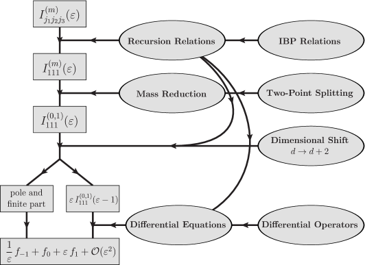
Figure 1: This flowchart provides an overview of the calculation of the $\varepsilon$-expansion of the general three-denominator angular integral $I_{j_{1}j_{2}j_{3}}^{(m)}$. In a first step, recursion relations (see app. C) derived from IBP relations (see sec. II) are used for a reduction to the master integral $I_{111}^{(m)}$. In a second step, the double- and triple-massive integrals are expressed in terms of massless and single-massive ones through mass reduction formulae derived from the two-point splitting lemma (see sec. III). In a third step, a combination of a dimensional-shift identity, relating integrals in $d$ and $d+2$ dimensions, with the recursion relations allows for the determination of pole and finite part in terms of known two-denominator integrals (see sec. IV). In a final step, the order $\varepsilon$ contribution is calculated by applying the method of differential equations – requiring suitable differential operators for angular integrals (see sec. V) and again making use of the recursion relations – to the massless and single-massive master integral in $d=6-2\varepsilon$ dimensions (see sec. VI and VII). Results are found in sec. VIII. Image created with JaxoDraw [46].

The remainder of the paper is organized as follows. In section II, we derive IBP relations to reduce $I_{j_{1},j_{2},j_{3}}$ to master integrals. Section III recalls the two-point splitting lemma, which allows us to express double- and triple-massive integrals in terms of the single-massive integral. The dimensional-shift identity introduced in section IV allows us to express the pole and finite part of the three-denominator integral solely in terms of known two-denominator integrals. In section V, we determine differential operators, which we subsequently use to derive differential equations for the master integrals in section VI. The integration of these differential equations is discussed in section VII. Results for the massless, single-massive, double-massive, and triple-massive master integrals $I^{(0,1,2,3)}_{111}$ are given in section VIII. The generalization towards angular integrals with more than three denominators is briefly discussed in section IX, before we conclude in section X. Appendix A lists the scalar products used for the mass reduction formula, while appendices B and C give the full form of the IBP relations and the recursion relations obtained from the latter. In appendix D, a proof of the general dimensional-shift identity for angular integrals is provided. Appendix E lists the expansions for the dimensionally-shifted two-denominator integrals that are used as input for the calculation of the three-denominator master integrals. The explicit calculation of the boundary value for the massless master integral is given in appendix F. Integrals useful for the calculation of the master integrals are found in appendix G, and appendix H recalls the Clausen function appearing in the order $\varepsilon$ of the three-denominator angular integrals. The ancillary Mathematica file provides the function AngularIntegral[{j1_,j2_,j3_},{v12_,v13_,v23_,v11_,v22_,v33_}] which evaluates the three-denominator angular integral in $d=4-2\varepsilon$ dimensions up to order $\varepsilon$.

II IBP relations

Since they are the foundation for everything that follows, we continue by deriving IBP relations to reduce $I_{j_{1},j_{2},j_{3}}$ to master integrals. IBP relations for angular integrals are derived in a similar fashion to loop integrals. The only difference is that permissible vectors in the IBP relation have to be tangential to the spherical integration surface. Concretely, the IBPs read

$$0=\int\mathrm{d}\Omega\frac{\partial}{\partial\vec{k}}\cdot\vec{\xi}\ \frac{1}{(v_{1}\cdot k)^{j_{1}}(v_{2}\cdot k)^{j_{2}}(v_{3}\cdot k)^{j_{3}}}\,,$$ (3)

where the vector $\vec{\xi}$ must satisfy $\vec{\xi}\cdot\vec{k}\overset{!}{=}0$.

To construct possible vectors $\vec{\xi}$ we can use the $\vec{v}_{i}$ as well as $\vec{k}$. From the orthogonality condition, we find the three vectors ($i=1,2,3$; note that $k$ is not an index)

$$\vec{\xi}_{ik}=(\vec{v}_{i}\cdot\vec{k})\vec{k}-\vec{k}^{2}\vec{v}_{i}$$ (4)

and the additional three vectors ($i<j$)

$$\vec{\xi}_{ij}=(\vec{v}_{i}\cdot\vec{k})\vec{v}_{j}-(\vec{v}_{j}\cdot\ \vec{k})\vec{v}_{i}\,.$$ (5)

For these vectors, it is

$$\frac{\partial\cdot\vec{\xi}_{ik}}{\partial\vec{k}}=(d-2)\vec{v}_{i}\cdot\vec{k}\quad\text{respectively}\quad\frac{\partial\cdot\vec{\xi}_{ij}}{\partial\vec{k}}=0$$ (6)

and furthermore, recalling $v_{i}\cdot k=1-\vec{v}_{i}\cdot\vec{k}$,

$$\frac{\partial}{\partial\vec{k}}\frac{1}{(v_{i}\cdot k)^{j_{i}}}=\frac{j_{i}\vec{v}_{i}}{(v_{i}\cdot k)^{j_{i}+1}}\,.$$ (7)

Applying the product rule, eq. (3) becomes

$$0=\int\mathrm{d}\Omega \left[\left(\frac{\partial\cdot\vec{\xi}}{\partial\vec{k}}\right)\frac{1}{(v_{1}\cdot k)^{j_{1}}(v_{2}\cdot k)^{j_{2}}(v_{3}\cdot k)^{j_{3}}}+\vec{\xi}\cdot\frac{\partial}{\partial\vec{k}}\frac{1}{(v_{1}\cdot k)^{j_{1}}(v_{2}\cdot k)^{j_{2}}(v_{3}\cdot k)^{j_{3}}}\right].$$ (8)

Using eqs. (6) and (7) on eq. (8) and expressing all scalar products in terms of (inverse) propagators leads to an IBP relation for each of the six $\vec{\xi}$. Those relate $I_{j_{1},j_{2},j_{3}}$ for different indices. We list them explicitly in appendix B.

For general $j_{1,2,3}$ these IBP relations can be combined into identities that only either raise or lower the sum of indices. This allows to bring them in the form of recursion relations that systematically reduce all integrals $I_{j_{1},j_{2},j_{3}}$ into the master integrals $I_{111}$, $I_{110}$, $I_{100}$, $I_{000}$ (+ permutation of indices), bypassing the need for Laporta’s algorithm [47]. The explicit recursion relations are given in appendix C.

To calculate the master integrals, we use the method of differential equations. For this, we write the master integrals in the form of eq. (1) and differentiate both sides with respect to the kinematic invariants $v_{ij}$, which will lead to new angular integrals on the right-hand side – details of the differentiation are discussed in section V. By reducing the right-hand side to master integrals via the recursion relations, we obtain a system of differential equations for the master integrals. For a pedagogical introduction to the differential equation approach in the context of loop integrals see [44, 45].

Since the $\varepsilon$-expansion of two-denominator angular integrals is known [3, 4, 5], the only unknown master integral in our case is $I_{111}$. By explicitly inserting the known integrals into the coupled system of differential equations, it is reduced to one closed differential equation for $I_{111}$.

To further simplify matters we use the following tricks:

• By two-mass splitting we can always reduce the triple-massive integral to single-massive integrals. We will be discussing this next in section III. This simplifies the differential equation by reducing the number of variables. The number of master integrals is further reduced since the massless one-denominator integral $I_{100}$ is reducible to $I_{000}$.

• By using a dimensional-shift identity $d\rightarrow d+2$ we obtain the pole and – somewhat surprisingly – also the finite part of the three-denominator integral “for free”, i.e. in terms of known integrals with fewer denominators. We will look at this in section IV.

• By symmetry it suffices to look at a single derivative, say ${\partial}/{\partial v_{12}}$, for the massless case. From there we only need a single boundary value for which we choose the symmetric point $v_{12}=v_{13}=v_{23}=1$. To construct the single-massive integral from the differential equation with respect to ${\partial}/{\partial v_{11}}$ we can use the previously calculated massless integral as a boundary condition. This will be done in sections VI and VII.

III Mass reduction via two-point splitting

It is a truth universally acknowledged, that a single-massive angular integral is sufficient to calculate multi-mass angular integrals. This is possible due to the two-point splitting lemma [5, 6], which states that for any two vectors $v_{1}$ and $v_{2}$, we can choose any scalar $\lambda_{(12)}$ and construct the linear combination ${v_{(12)}\equiv(1-\lambda_{(12)})\,v_{1}+\lambda_{(12)}\,v_{2}}$ to obtain

$$\frac{1}{v_{1}\cdot k\,\,v_{2}\cdot k}=\frac{\lambda_{(12)}}{v_{1}\cdot k\,\,v_{(12)}\cdot k}+\frac{1-\lambda_{(12)}}{v_{2}\cdot k\,\,v_{(12)}\cdot k}\,.$$ (9)

If we consider two massive vectors $v_{1}$ and $v_{2}$ and choose $\lambda_{(12)}$ such that $v_{(12)}$ is massless, i.e. $v_{(12)(12)}=0$, eq.(9) splits the product of two massive denominators into the sum of two single-massive denominator products. Iterative use of this identity on pairs of massive denominators allows for a reduction to the single-massive case. Hence angular integrals with an arbitrary number of masses can always be expressed through at most single-massive integrals. 

Solving the masslessness condition $v_{(12)(12)}\overset{!}{=}0$ for $\lambda_{(12)}$ yields the solutions

$$\lambda_{(12)}^{\pm}=\frac{v_{12}-v_{11}\pm\sqrt{v_{12}^{2}-v_{11}v_{22}}}{2v_{12}-v_{11}-v_{22}}\,.$$ (10)

Both of these solutions can be used for a reduction of the number of masses. To make the reduction well-behaved in the massless limit we can bring eq.(9) into symmetric form by introducing the additional vector $v_{(21)}\equiv\lambda_{(21)}\,v_{1}+(1-\lambda_{(21)})\,v_{2}$. Employing the two-point splitting lemma  (9) first on $1/(v_{1}\cdot k\,v_{2}\cdot k)$ inserting $v_{(12)}$ and subsequently on $1/(v_{2}\cdot k\,v_{(12)}\cdot k)$ inserting $v_{(21)}$, we obtain the splitting

$$\frac{1}{v_{1}\cdot k\,\,v_{2}\cdot k}= \frac{\lambda_{(12)}}{v_{1}\cdot k\,\,v_{(12)}\cdot k}+\frac{\lambda_{(21)}}{v_{2}\cdot k\,\,v_{(21)}\cdot k}+\frac{1-\lambda_{(12)}-\lambda_{(21)}}{v_{(12)}\cdot k\,\,v_{(21)}\cdot k}\,.$$ (11)

To make $v_{(12)}$ and $v_{(21)}$ massless as well as coinciding with $v_{1}$ respectively $v_{2}$ in the respective massless limit, we choose

$$\lambda_{(12)}=\frac{v_{12}-v_{11}-\sqrt{X_{12}}}{2v_{12}-v_{11}-v_{22}}\,,\quad\lambda_{(21)}=\frac{v_{12}-v_{22}-\sqrt{X_{12}}}{2v_{12}-v_{11}-v_{22}}\,,$$ (12)

with $X_{12}\equiv v_{12}^{2}-v_{11}v_{22}$. Note that there is the geometrical interpretation $X_{12}=4\,\mathbb{V}(\vec{v}_{1},\vec{v}_{2})^{2}+(\vec{v}_{1}-\vec{v}_{2})^{2}$, where $\mathbb{V}(\vec{v}_{1},\vec{v}_{2})$ denotes the area of the triangle spanned by $\vec{v}_{1}$ and $\vec{v}_{2}$. Hence, for real vectors $\vec{v}_{1,2}$, $X_{12}$ is non-negative and vanishes if and only if $\vec{v}_{1}=\vec{v}_{2}$. The scalar products of the auxiliary vectors are ${v_{(12)(12)}=v_{(21)(21)}=0}$, ${v_{1(12)}=-\lambda_{(12)}\sqrt{X_{12}}}$, ${v_{2(21)}=-\lambda_{(21)}\sqrt{X_{12}}}$, and ${v_{(12)(21)}=2X_{12}/(2v_{12}-v_{11}-v_{22})}$. Note that $v_{1(12)}$ respectively $v_{2(21)}$ vanish in the massless limits $v_{11}\rightarrow 0$ respectively $v_{22}\rightarrow 0$ . Using these scalar products, a compact form of the two-mass splitting is

$$\frac{1}{v_{1}\cdot k\,\,v_{2}\cdot k}= \frac{1}{\sqrt{X_{12}}}\left[\frac{v_{(12)(21)}}{v_{(12)}\cdot k\,\,v_{(21)}\cdot k}-\frac{v_{1(12)}}{v_{1}\cdot k\,\,v_{(12)}\cdot k}-\frac{v_{2(21)}}{v_{2}\cdot k\,\,v_{(21)}\cdot k}\right].$$ (13)

The reduction formula for the double-massive master integral immediately following from this is

$$I_{111}^{(2)}(v_{12},v_{13},v_{23},v_{11},v_{22})=\frac{1}{\sqrt{X_{12}}} \left[v_{(12)(21)}I_{111}^{(0)}\left(v_{3(12)},v_{3(21)},v_{(12)(21)}\right)-v_{1(12)}I_{111}^{(1)}\left(v_{13},v_{1(12)},v_{3(12)},v_{11}\right)\right..$$

$$\left.-v_{2(21)}I_{111}^{(1)}\left(v_{23},v_{2(21)},v_{3(21)},v_{22}\right)\right]$$ (14)

In case $v_{3}$ is massive as well, eq.(11) is applied twice to obtain the following reduction formula for the triple-massive master integral

$$I_{111}^{(3)} (v_{12},v_{13},v_{23},v_{11},v_{22},v_{33})=\frac{1}{\sqrt{X_{12}}}\Big{\{}v_{(12)(21)}I_{111}^{(1)}\left(v_{3(12)},v_{3(21)},v_{(12)(21)},v_{33}\right)$$

$$-\frac{v_{1(12)}}{\sqrt{X_{13}}}\Big{[}v_{(13)(31)}I_{111}^{(0)}\left(v_{(12)(13)},v_{(12)(31)},v_{(13)(31)}\right)-v_{1(13)}I_{111}^{(1)}\left(v_{1(12)},v_{1(13)},v_{(12)(13)},v_{11}\right)$$

$$\qquad-v_{3(31)}I_{111}^{(1)}\left(v_{3(12)},v_{3(31)},v_{(12)(31)},v_{33}\right)\Big{]}$$

$$-\frac{v_{2(21)}}{\sqrt{X_{23}}}\Big{[}v_{(23)(32)}I_{111}^{(0)}\left(v_{(21)(23)},v_{(21)(32)},v_{(23)(32)}\right)-v_{2(23)}I_{111}^{(1)}\left(v_{2(21)},v_{2(23)},v_{(21)(23)},v_{22}\right)$$

$$\qquad-v_{3(32)}I_{111}^{(1)}\left(v_{3(21)},v_{3(32)},v_{(21)(32)},v_{33}\right)\Big{]}\Big{\}}\,,$$ (15)

where the explicit expressions for the scalar products that appear are listed in appendix A. In principle one could derive reduction formulae for any integer indices $j_{i}$, however in light of the recursion relations derived in the previous section and given in appendix C this is not required.

We note that we can present the mass reduction formulae in a much cleaner form by scaling the three-denominator integrals by their Euclidean Gram determinant

$$Y_{ijk}=\det\!\left(\begin{array}[]{ccc}1-v_{ii}&1-v_{ij}&1-v_{ik}\\ 1-v_{ij}&1-v_{jj}&1-v_{jk}\\ 1-v_{ik}&1-v_{jk}&1-v_{kk}\end{array}\right).$$ (19)

Defining

$$\tilde{I}^{(m)}_{111}(v_{ij},v_{ik},v_{jk},v_{ii},v_{jj},v_{kk})\equiv\sqrt{Y_{ijk}}\,I^{(m)}_{111}(v_{ij},v_{ik},v_{jk},v_{ii},v_{jj},v_{kk})\,,$$ (20)

the two-mass reduction formula (14) takes the form

$$\tilde{I}_{111}^{(2)}(v_{12},v_{13},v_{23},v_{11},v_{22})=\tilde{I}_{111}^{(0)}\left(v_{3(12)},v_{3(21)},v_{(12)(21)}\right)-\tilde{I}_{111}^{(1)}\left(v_{13},v_{1(12)},v_{3(12)},v_{11}\right)-\tilde{I}_{111}^{(1)}\left(v_{23},v_{2(21)},v_{3(21)},v_{22}\right),$$ (21)

which remarkably is free of explicit kinematic prefactors. This generalizes to the three-mass reduction (15) which for the scaled angular integrals becomes

$$\tilde{I}_{111}^{(3)} (v_{12},v_{13},v_{23},v_{11},v_{22},v_{33})=\tilde{I}_{111}^{(1)}\left(v_{3(12)},v_{3(21)},v_{(12)(21)},v_{33}\right)-\tilde{I}_{111}^{(0)}\left(v_{(12)(13)},v_{(12)(31)},v_{(13)(31)}\right)$$

$$+\tilde{I}_{111}^{(1)}\left(v_{1(12)},v_{1(13)},v_{(12)(13)},v_{11}\right)+\tilde{I}_{111}^{(1)}\left(v_{3(12)},v_{3(31)},v_{(12)(31)},v_{33}\right)-\tilde{I}_{111}^{(0)}\left(v_{(21)(23)},v_{(21)(32)},v_{(23)(32)}\right)$$

$$+\tilde{I}_{111}^{(1)}\left(v_{2(21)},v_{2(23)},v_{(21)(23)},v_{22}\right)+\tilde{I}_{111}^{(1)}\left(v_{3(21)},v_{3(32)},v_{(21)(32)},v_{33}\right).$$ (22)

IV Dimensional-shift identity

The $n$-denominator angular integral satisfies the general dimensional-shift identity

$$I_{j_{1},...,j_{n}}(\varepsilon)= \frac{1}{1-2\varepsilon}\left[\sum_{i=1}^{n}j_{i}I_{j_{1},...,j_{i}+1,...,j_{n}}(\varepsilon-1)+\,\left(3-\sum_{i=1}^{n}j_{i}-2\varepsilon\right)I_{j_{1},...,j_{n}}(\varepsilon-1)\right],$$ (23)

which expresses the integral in $d=4-2\varepsilon$ dimensions on the left side as a sum over integrals in $d+2=6-2\varepsilon$ dimensions on the right. A proof of eq. (23) is given in appendix D.

In combination with IBP reduction, this identity can be used to analytically continue the angular integral from a convergent dimension to a divergent one. Note that for the three-denominator angular integral already the angular measure as defined in eq. (2) is divergent in $d=4$ dimensions due to the $\sin^{-1}\theta_{3}$ factor. With the above formula we can however express the integral in $d=4$ dimensions in terms of integrals in $d=6$ dimensions where the measure is finite because it contains an additional $\sin^{2}\theta_{3}$ factor.

Also the master integrals with $j_{i}=1$ and $v_{ii}=0$, which are collinearly divergent in $d=4$ dimensions, converge for sufficiently large dimension, i.e. small $\varepsilon$. In particular they are finite in $d=6$ dimensions. Hence applying eq.(23) to $I_{111}(\varepsilon)$ and subsequently reducing the integrals in six dimensions on the right to master integrals, results in all $1/\varepsilon$ poles being captured in prefactors of the master integrals.

As it turns out the identity connecting $I_{111}(\varepsilon)$ and $I_{111}(\varepsilon-1)$ simplifies further by shifting all integrals with two or less denominators back to $d=4-2\varepsilon$ dimensions. The necessary identities follow from eq.(23) by subsequently choosing zero, one, and two denominators, performing an IBP reduction and solving for the $d=6-2\varepsilon$ dimensional integrals. Going through the outlined steps, we find the remarkably simple relation

$$I_{111}(\varepsilon)=\frac{1}{X_{123}}\left[X_{12\bar{3}}I_{110}(\varepsilon)+X_{1\bar{2}3}\,I_{101}(\varepsilon)+X_{\bar{1}23}\,I_{011}(\varepsilon)+\frac{2\varepsilon}{1-2\varepsilon}\,Y_{123}\,I_{111}(\varepsilon-1)\right].$$ (24)

The kinematic factor $X_{123}$ in this relation is given by the (Minkowski-)Gram determinant

$$X_{123}\equiv \det\!\left(\begin{array}[]{ccc}v_{11}&v_{12}&v_{13}\\ v_{12}&v_{22}&v_{23}\\ v_{13}&v_{23}&v_{33}\end{array}\right)=2v_{12}v_{13}v_{23}-v_{11}v_{23}^{2}-v_{13}^{2}v_{22}-v_{33}v_{12}^{2}+v_{11}v_{22}v_{33}\,.$$ (28)

The factors $X_{12\bar{3}}$, $X_{1\bar{2}3}$, and $X_{\bar{1}23}$ multiplying the two-denominator integrals are obtained by interchanging the barred column in the Gram matrix with a column of ones , i.e.

$$X_{12\bar{3}}\equiv\det\!\left(\begin{array}[]{ccc}v_{11}&v_{12}&1\\ v_{12}&v_{22}&1\\ v_{13}&v_{23}&1\end{array}\right)=v_{12}(v_{13}+v_{23}-v_{12})-v_{11}v_{23}-v_{22}v_{13}+v_{11}v_{22},$$ (32)

for $X_{1\bar{2}3}$ and $X_{\bar{1}23}$ indices are interchanged cyclically. The factor $Y_{123}$ is given by the Euclidean Gram determinant already encountered in eq. (19),

$$Y_{123}= 2v_{12}v_{13}+2v_{12}v_{23}+2v_{13}v_{23}-v_{12}^{2}-v_{13}^{2}-v_{23}^{2}-2v_{12}v_{13}v_{23}-v_{11}v_{23}(2-v_{23})-v_{22}v_{13}(2-v_{13})$$

$$-v_{33}v_{12}(2-v_{12})+v_{11}v_{22}+v_{11}v_{33}+v_{22}v_{33}-v_{11}v_{22}v_{33}\,.$$ (33)

Note, that geometrically

$$Y_{123}=\beta_{1}^{2}\beta_{2}^{2}\beta_{3}^{2}\sin^{2}\chi_{2}^{(1)}\sin^{2}\chi_{3}^{(1)}\sin^{2}\chi_{3}^{(2)}=36\,\mathbb{V}^{2}(\vec{v}_{1},\vec{v}_{2},\vec{v}_{3})$$ (34)

where $\mathbb{V}(\vec{v}_{1},\vec{v}_{2},\vec{v}_{3})$ denotes the Euclidean volume of the tetrahedron spanned by the vectors $\vec{v}_{1,2,3}$. We note that for real valued vectors $\vec{v}_{i}$ the quantity $Y_{123}$ appearing in the denominator vanishes if and only if the vectors are confined to a plane, i.e. they are linearly dependent. In this particular case eq. (24) becomes a reduction identity of the three-denominator integral to a sum of two-denominator integrals – remarkably the very same, one would also find by partial fractioning of the integrand.

Using the formula (24) has two benefits. Firstly for the purpose of analytical calculation, we gain the pole part and the $\varepsilon^{0}$ term “for free” since they are contained entirely in terms of known two-denominator integrals. Since $I_{111}(\varepsilon-1)$ is finite for $\varepsilon=0$ and is multiplied by an explicit $\varepsilon$ in eq. (24), it only starts contributing at order $\varepsilon$. Hence, for results to order $\varepsilon$ it suffices to calculate the leading term of $I_{111}(\varepsilon-1)$ by differential equations.

Secondly, from a numerical perspective, by expanding the integration measure of $I_{111}(\varepsilon-1)$ in a series in $\varepsilon$ we obtain a finite integral representation for every order in $\varepsilon$. In conjunction with the known expansion of the two-denominator integrals this can be used for numeric checks.

V Differential operators for angular integrals

To derive differential equations with respect to the scalar products $v_{ij}$, we need to differentiate

$$\int\mathrm{d}\Omega\,\frac{1}{(v_{1}\cdot k)^{j_{1}}(v_{2}\cdot k)^{j_{2}}(v_{3}\cdot k)^{j_{3}}}\,,$$ (35)

which however depends on the explicit vectors $\vec{v}_{i}$. Thus, the first step is to derive appropriate differential operators. Due to symmetry, it is sufficient to consider the derivatives with respect to $v_{12}=1-\vec{v}_{1}\cdot\vec{v}_{2}$ respectively the mass $v_{11}=1-\vec{v}_{1}\cdot\vec{v}_{1}$. For this we make the ansätze

$$\frac{\partial}{\partial v_{12}}\overset{!}{=}(a_{1}\vec{v}_{1}+a_{2}\vec{v}_{2}+a_{3}\vec{v}_{3})\cdot\frac{\partial}{\partial\vec{v_{1}}}\,\quad\text{respectively}\quad\frac{\partial}{\partial v_{11}}\overset{!}{=}(b_{1}\vec{v}_{1}+b_{2}\vec{v}_{2}+b_{3}\vec{v}_{3})\cdot\frac{\partial}{\partial\vec{v_{1}}}\,.$$ (36)

The coefficients $a_{1,2,3}$ and $b_{1,2,3}$ are fixed by the conditions

$$\frac{\partial v_{11}}{\partial v_{12}}=0\,,\quad\frac{\partial v_{12}}{\partial v_{12}}=1\,,\quad\frac{\partial v_{13}}{\partial v_{12}}=0\quad\text{respectively}\quad\frac{\partial v_{11}}{\partial v_{11}}=1\,,\quad\frac{\partial v_{12}}{\partial v_{11}}=0\,,\quad\frac{\partial v_{13}}{\partial v_{11}}=0\,.$$ (37)

Derivatives of the other invariants $v_{22}$, $v_{23}$, $v_{33}$ are trivially $0$ due to the chosen ansatz. For $\partial/\partial v_{12}$, in the massless case, where $v_{11}=v_{22}=v_{33}=0$, we find

$$\frac{\partial}{\partial v_{12}}=\frac{1}{Y_{123}^{(0)}}\Big{[}(v_{13}+v_{23}-v_{12}-v_{13}v_{23})\vec{v}_{1}-(2-v_{13})v_{13}\vec{v}_{2}+(v_{12}+v_{13}-v_{23}-v_{12}v_{13})\vec{v}_{3}\Big{]}\cdot\frac{\partial}{\partial\vec{v}_{1}},$$ (38)

where in the massless case the denominator is given by

$$Y_{123}^{(0)}= -v_{12}^{2}-v_{13}^{2}-v_{23}^{2}+2v_{12}v_{13}+2v_{12}v_{23}+2v_{13}v_{23}-2v_{12}v_{13}v_{23},$$ (39)

which is the massless Euclidean Gram determinant from eq. (33). Of course the operator can be generalized to the case of non-zero masses, however this is not needed in the following. The differential operators $\partial/\partial v_{13}$ and $\partial/\partial v_{23}$ follow by interchanging indices.

For the differential operator $\partial/\partial v_{11}$ we find in the single-massive case $v_{22}=v_{33}=0$

$$\frac{\partial}{\partial v_{11}}=\frac{1}{2Y_{123}^{(1)}}\Big{[}-v_{23}(2-v_{23})\vec{v}_{1}+(v_{13}+v_{23}-v_{12}-v_{13}v_{23})\vec{v}_{2}+(v_{12}+v_{23}-v_{13}-v_{12}v_{13})\vec{v}_{3}\Big{]}\cdot\frac{\partial}{\partial\vec{v}_{1}},$$ (40)

where the denominator is given by

$$Y_{123}^{(1)}=Y_{123}^{(0)}-v_{11}v_{23}(2-v_{23})\,.$$ (41)

Again we recognize the Euclidean Gram determinant from eq. (33), this time for one non-zero mass.

VI Differential equations

Having constructed suitable differential operators we are now equipped to derive differential equations for the three-denominator angular integral. The only master integral with genuinely three denominators is $I_{111}$. All other master integrals have at most two denominators and are known to all orders in $\varepsilon$. To construct the full solution for an arbitrary number of masses, we have to look at two cases. First we consider the massless integral. It is symmetric in its variables $v_{12},v_{13},v_{23}$, hence it suffices to only consider the differential equation $\partial/\partial v_{12}$ and construct a symmetric solution. As a boundary value we will use the integral at the symmetric point $v_{12}=v_{13}=v_{23}=1$. The second case to consider is the single-massive integral with $v_{11}\neq 0$. Here, we look at the differential equation with respect to $\partial/\partial v_{11}$ and use the massless integral as a boundary condition. As discussed in section IV it is beneficial to consider the differential equations for integrals in $d=6-2\varepsilon$ dimensions. This way, the leading-order solution in $\varepsilon$ of the differential equation, which is of order $\varepsilon^{0}$, will provide a contribution to the order $\varepsilon$ of the master integral in $d=4-2\varepsilon$ dimensions.

By applying the differential operators to the massless integral, we obtain

$$\frac{\partial I^{(0)}_{111}}{\partial v_{12}}=\frac{1}{Y_{123}^{(0)}} \Big{[}v_{13}(v_{13}-v_{12}-v_{23})I^{(0)}_{211}+(v_{12}-v_{13}-v_{23}+v_{13}v_{23})I^{(0)}_{111}+v_{13}(2-v_{13})I^{(0)}_{201}$$

$$+(v_{23}-v_{12}-v_{13}+v_{12}v_{13})I^{(0)}_{210}\Big{]}$$ (42)

and for the single-massive integral

$$\frac{\partial I^{(1)}_{111}}{\partial v_{11}}=\frac{1}{2Y_{123}^{(1)}} \Big{[}v_{23}(v_{23}-v_{12}-v_{13})I^{(1)}_{211}+v_{23}(2-v_{23})I^{(1)}_{111}+(v_{13}-v_{12}-v_{23}+v_{12}v_{23})I^{(1)}_{210}$$

$$+(v_{12}-v_{13}-v_{23}+v_{13}v_{23})I^{(1)}_{201}\Big{]}.$$ (43)

From here, we can use the recursion relations from appendix C to reduce the right-hand side of both equations to master integrals. In both cases, this results in a closed differential equation for $I_{111}$, where all other terms are expressed in terms of known lower-denominator integrals.

The reduction to master integrals of the massless equation in $d$ dimensions leads to

$$\frac{\partial I^{(0)}_{111}}{\partial v_{12}}=\left[\frac{d-6}{2v_{12}}-\frac{d-5}{Y_{123}^{(0)}}\,(v_{13}+v_{23}-v_{23}-v_{13}v_{23})\right] I^{(0)}_{111}+\frac{1}{2v_{12}Y_{123}^{(0)}}\Big{[}(d-5)v_{12}(4-v_{12}-v_{13}-v_{23})I^{(0)}_{110}$$

$$+(d-5)(2-v_{13})(v_{23}-v_{12}-v_{13}) I^{(0)}_{101}+(d-5)(2-v_{23})(v_{13}-v_{12}-v_{23})I^{(0)}_{011}\Big{]}.$$ (44)

Analogously, the single-massive differential equation becomes

$$\frac{\partial I^{(1)}_{111}}{\partial v_{11}} =\left[\frac{(6-d)v_{23}}{2(2v_{12}v_{13}-v_{11}v_{23})}+\frac{(d-5)v_{23}(2-v_{23})}{2Y_{123}^{(1)}}\right]I^{(1)}_{111}$$

$$+\frac{d-5}{2Y_{123}^{(1)}(2v_{12}v_{13}-v_{11}v_{23})}\Big{[}\Big{(}(v_{12}+v_{13}-v_{23})(v_{12}+v_{23}-v_{13}-v_{12}v_{23})+Y_{123}^{(1)}\Big{)}I_{110}^{(1)}$$

$$+\Big{(}(v_{12}+v_{13}-v_{23})(v_{13}+v_{23}-v_{12}-v_{13}v_{23})+Y_{123}^{(1)}\Big{)}I_{101}^{(1)}-(v_{12}+v_{13}-v_{23})v_{23}(2-v_{23})I_{011}^{(0)}\Big{]}$$

$$+\frac{(d-4)(1-v_{11})}{v_{11}(2v_{12}v_{13}-v_{11}v_{23})}I_{100}^{(1)}+\frac{3-d}{v_{11}(2v_{12}v_{13}-v_{11}v_{23})}I_{000}^{(0)}\,.$$ (45)

We note that in both eqs. (44) and (45) all master integrals except for $I_{111}^{(0,1)}$ are known analytically in $d$ dimensions.

As discussed in section IV, it is most useful to consider the differential equations in $d=6-2\varepsilon$ dimensions. The standard procedure to approach differential equations of this form is bringing them to canonical $\varepsilon$-form, i.e. making the coefficient in front of $I_{111}$ proportional to $\varepsilon$. In the particular case at hand we can even make the entire coefficient disappear, leaving us with a right-hand side which is expressed solely in terms of known integrals This is achieved by rescaling the integral to $J_{111}=f(v)I_{111}$. Schematically writing the original eqs. (44) and (45) as

$$\frac{\partial I_{111}}{\partial v}\,=\,c(v)\,I_{111}\,+\,r(v)\,,$$ (46)

the corresponding differential equation for the rescaled integral is

$$\frac{\partial J_{111}}{\partial v}\,=\left(\frac{1}{f(v)}\frac{\partial f(v)}{\partial v}\,+\,c(v)\right)J_{111}\,+\,f(v)\,r(v)\,.$$ (47)

Choosing ${f(v)=f_{0}\exp\left[-\int\mathrm{d}v\,c(v)\right]}$, the term in parentheses vanishes.

Explicitly, we rescale the massless integral as

$$J_{111}^{(0)} \equiv(v_{12}v_{13}v_{23})^{\varepsilon}\left(Y^{(0)}_{123}\right)^{1/2-\varepsilon}I_{111}^{(0)}.$$ (48)

The prefactor is chosen such that in the differential equation for $\partial/\partial v_{12}J_{111}^{(0)}$ the coefficient in front of $J_{111}^{(0)}$ becomes zero while simultaneously preserving the symmetry between variables. For the single-massive integral we rescale as

$$J_{111}^{(1)} \equiv\left(\frac{v_{23}}{2}\right)^{\varepsilon}(2v_{12}v_{13}-v_{11}v_{23})^{\varepsilon}\left(Y^{(1)}_{123}\right)^{1/2-\varepsilon}I_{111}^{(1)}\,,$$ (49)

making the coefficient in front of $J_{111}^{(1)}$ vanish in the differential equation for $\partial/\partial v_{11}J_{111}^{(1)}$ and also preserving the property that $J^{(1)}_{111}$ reduces to $J^{(0)}_{111}$ in the massless limit.

Explicitly we find in the massless case

$$\frac{\partial J^{(0)}_{111}(\varepsilon-1)}{\partial v_{12}}= (v_{12}v_{13}v_{23})^{\varepsilon}\left(Y^{(0)}_{123}\right)^{-1/2-\varepsilon}\frac{1-2\varepsilon}{2\,v_{12}}\Big{[}v_{12}(4-v_{12}-v_{13}-v_{23})I^{(0)}_{110}(\varepsilon-1)$$

$$+(2-v_{13})(v_{23}-v_{12}-v_{13})I^{(0)}_{101}(\varepsilon-1)+(2-v_{23})(v_{13}-v_{12}-v_{23})I^{(0)}_{011}(\varepsilon-1)\Big{]}.$$ (50)

This constitutes a closed-form expression for ${\partial J^{(0)}_{111}(\varepsilon-1)}/{\partial v_{12}}$ since the two-denominator integrals are known analytically in terms of hypergeometric functions as well as in terms of an all-order $\varepsilon$-expansion.

For the derivative ${\partial J^{(1)}_{111}(\varepsilon-1)}/{\partial v_{11}}$ we find a similar closed-form expression. Here, it is convenient to express the right-hand side in terms of $I^{(1)}_{200}$ instead of $I^{(1)}_{100}$ to make spurious poles in $1/v_{11}$ cancel between coefficients, thus allowing for an integration starting at the massless point $v_{11}=0$. Using the identity

$$I_{100}(v_{11};\varepsilon-1)=\frac{1}{2-2\varepsilon}\left[(3-2\varepsilon)I_{000}(\varepsilon-1)-v_{11}\,I_{200}(v_{11};\varepsilon-1)\right]$$ (51)

to substitute $I_{100}$ for $I_{200}$, the derivative of $J_{111}^{(1)}$ becomes

$$\frac{\partial J_{111}^{(1)}(\varepsilon-1)}{\partial v_{11}}= 2^{-1-\varepsilon}v_{23}^{\varepsilon}(2v_{12}v_{13}-v_{11}v_{23})^{-1+\varepsilon}\left(Y_{123}^{(1)}\right)^{-1/2-\varepsilon}$$

$$\times\Big{[}(1-2\varepsilon)\Big{(}(v_{12}+v_{13}-v_{23})(v_{12}+v_{23}-v_{13}-v_{12}v_{23})+Y_{123}^{(1)}\Big{)}\,I_{110}^{(1)}(\varepsilon-1)$$

$$\quad+(1-2\varepsilon)\Big{(}(v_{12}+v_{13}-v_{23})(v_{13}+v_{23}-v_{12}-v_{13}v_{23})+Y_{123}^{(1)}\Big{)}\,I_{101}^{(1)}(\varepsilon-1)$$

$$\quad-(1-2\varepsilon)(v_{12}+v_{13}-v_{23})v_{23}(2-v_{23})\,I_{011}^{(0)}(\varepsilon-1)$$

$$\quad-2(1-v_{11})Y_{123}^{(1)}\,I_{200}^{(1)}(\varepsilon-1)-2(3-2\varepsilon)Y_{123}^{(1)}\,I_{000}^{(0)}(\varepsilon-1)\Big{]}.$$ (52)

All functions on the right-hand side of this equation are known to all orders in $\varepsilon$.

VII Integration for master integrals

VII.1 Massless integral

To obtain the order $\varepsilon$ for $I_{111}^{(0)}$ in $d=4-2\varepsilon$ dimensions we only need the leading term of eq. (50) which is of order $\varepsilon^{0}$. Hence, we can set $\varepsilon=0$ in this equation and plug in the massless two-denominator integral in $d=6$ dimensions. Here we use the dimensionally-shifted massless two-denominator master integral given in eq. (106) of appendix E leading to

$$\frac{\partial J^{(0)}_{111}(-1)}{\partial v_{12}}=\frac{\pi}{\sqrt{Y_{123}^{(0)}}}\left[\log\frac{v_{13}v_{23}}{4}-\log\frac{v_{12}}{2}+\frac{(v_{13}-v_{23})\log\frac{v_{13}}{v_{23}}}{v_{12}}-\frac{(2-v_{13}-v_{23})\log\frac{v_{12}}{2}}{2-v_{12}}\right]\equiv j^{(0)}(v_{12},v_{13},v_{23})\,.$$ (53)

To obtain $J^{(0)}_{111}$ at a general kinematic point, we may choose the integration path $(1,1,1)\rightarrow(1,1,v_{23})\rightarrow(1,v_{13},v_{23})\rightarrow(v_{12},v_{13},v_{23})$ with boundary condition at the symmetric point $v_{12}=v_{13}=v_{23}=1$. The configuration of vectors used for the boundary value and the integration path are depicted in figure 2. By explicit calculation, the necessary boundary value is found to be

$$J^{(0),d=6}_{111}(1,1,1)=I^{(0),d=6}_{111}(1,1,1)=2\pi\,\mathrm{C}\,,$$ (54)

where $\mathrm{C}=\sum_{n=0}^{\infty}\frac{(-1)^{n}}{(2n+1)^{2}}$ denotes Catalan’s constant. Details of the calculation can be found in appendix F.

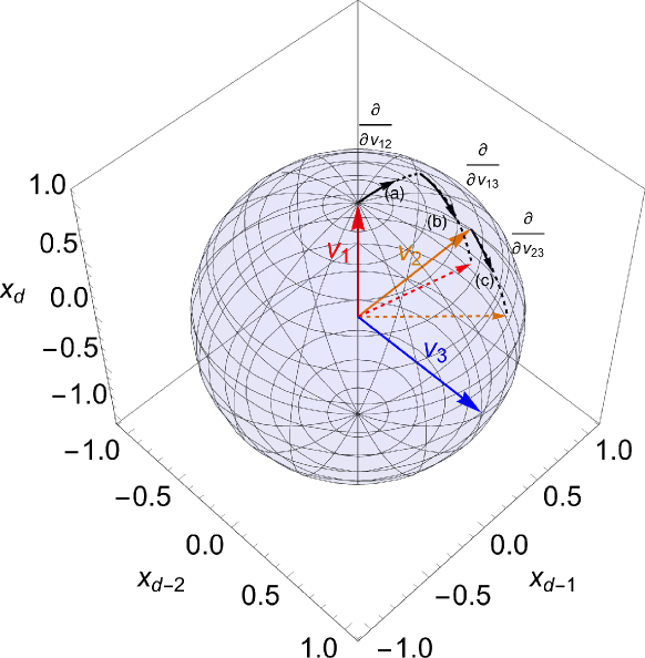
Figure 2: Illustration of the initial condition and the integration path for the massless three-denominator angular integral depending on vectors $v_{1,2,3}$. The plot shows the slice $x_{0}=1$ of $d$-dimensional Minkowski space. The blue unit sphere depicts the intersection with the light-cone, where $v^{2}=0$. The symmetric configuration showcased by the solid arrows is used as the boundary value. In this configuration $I_{111}^{(0)}(1,1,1)=2\pi\mathrm{C}$, where $\mathrm{C}$ denotes Catalan’s constant. The dashed black lines showcase the integration path. First, we rotate $v_{1}$ along path $(a)$, which is in the direction of $\partial/\partial v_{12}$. The axis of rotation is along $v_{3}$. Second, we rotate $v_{1}$ along path $(b)$, which is in the direction of $\partial/\partial v_{13}$. The axis of rotation is along $v_{2}$. Third, we rotate $v_{2}$ along path $(c)$, which is in the direction of $\partial/\partial v_{23}$, reaching the final configuration with general $v_{12}$, $v_{13}$, $v_{23}$. The axis of rotation is the rotated $v_{1}$ shown in dashed red. Note that the volume of the tetrahedron spanned by the vectors $v_{1,2,3}$ in this subspace is proportional to $\sqrt{Y_{123}^{(0)}}$ .

Utilizing the symmetry of the massless integral it is

$$J^{(0),d=6}_{111}(v_{12},v_{13},v_{23})=\int_{1}^{v_{12}}\!\!\!\!\mathrm{d}v\,j^{(0)}(v,v_{13},v_{23})+\int_{1}^{v_{13}}\!\!\!\!\mathrm{d}v\,j^{(0)}(v,1,v_{23})+\int_{1}^{v_{23}}\!\!\!\!\mathrm{d}v\,j^{(0)}(v,1,1)+J^{(0),d=6}_{111}(1,1,1)\,.$$ (55)

We note that alternatively $J_{111}^{(0)}$ is also fixed by being the unique symmetric solution to eq. (53) with the boundary condition (54).

To evaluate the integrals from (55) in terms of (generalized) polylogarithms, the only remaining obstacle is the presence of the square root $\sqrt{Y_{123}^{(0)}}$. A general algorithmic approach to rationalize roots of this kind has been presented in [49]. In the present case the required change of variables is $v_{12}\rightarrow u$ with

$$v_{12}=\frac{v_{+}+v_{-}u^{2}}{1+u^{2}}\quad\text{and Jacobian }\frac{\mathrm{d}v_{12}}{\mathrm{d}u}=-\frac{2u(v_{+}-v_{-})}{(1+u^{2})^{2}}\,,$$ (56)

where $v_{\pm}$ are defined such that they factorize the square root, i.e. $Y_{123}^{(0)}=(v_{+}-v_{12})(v_{12}-v_{-})$, explicitly

$$v_{\pm}\equiv v_{13}+v_{23}-v_{13}v_{23}\pm\sqrt{v_{13}(2-v_{13})v_{23}(2-v_{23})}\,.$$ (57)

The square root of the Gram determinant becomes in the new variable $u$

$$Y_{123}^{(0)}=\frac{2u}{1+u^{2}}\,\sqrt{v_{13}(2-v_{13})v_{23}(2-v_{23})}\,.$$ (58)

The integrals resulting from this change of variables take the form of $J_{0}(\delta)$ and $J_{2}(\beta,\delta)$ defined in appendix G. After considerable simplifications between the terms we obtain the result given in section VIII.1.

VII.2 Single-massive integral

To obtain the order $\varepsilon$ for $I_{111}^{(1)}$ in $d=4-2\varepsilon$ dimensions we only need the leading $\varepsilon^{0}$ term of eq. (52). Hence, we can again simply put $\varepsilon=0$ in this equation and plug in the known integrals with two and fewer denominators in $d=6$. Besides eq.(106) we use the dimensionally-shifted two-denominator integrals from appendix E leading to

$$\frac{\partial J_{111}^{(1)}(-1)}{\partial v_{11}}=\frac{\pi}{\sqrt{Y_{123}^{(1)}}} \left[\frac{(v_{12}-1)(v_{12}+v_{23}-v_{13}-v_{12}v_{23})\log\!\left(\frac{1+\sqrt{1-v_{11}}}{1-\sqrt{1-v_{11}}}\right)}{2(v_{12}(2-v_{12})-v_{11})\sqrt{1-v_{11}}}\right.$$

$$+\frac{(v_{13}-1)(v_{13}+v_{23}-v_{12}-v_{13}v_{23})\log\!\left(\frac{1+\sqrt{1-v_{11}}}{1-\sqrt{1-v_{11}}}\right)}{2(v_{13}(2-v_{13})-v_{11})\sqrt{1-v_{11}}}+\frac{(v_{12}+v_{23}-v_{13}-v_{12}v_{23})\log\frac{v_{11}}{v_{12}^{2}}}{2(v_{12}(2-v_{12})-v_{11})}$$

$$+\frac{(v_{13}+v_{23}-v_{12}-v_{13}v_{23})\log\frac{v_{11}}{v_{13}^{2}}}{2(v_{13}(2-v_{13})-v_{11})}\left.+\frac{(v_{12}+v_{13}-v_{23})v_{23}\log\!\left(\frac{v_{11}v_{23}}{2v_{12}v_{13}}\right)}{2v_{12}v_{13}-v_{11}v_{23}}\right]\equiv j^{(1)}(v_{11})\,.$$ (59)

Integrating the right-hand side starting at $v_{11}=0$ we can use the massless integral $J^{(0),d=6}_{111}$ as a boundary value,

$$J_{111}^{(1),d=6}(v_{11})=J_{111}^{(0),d=6}+\int_{0}^{v_{11}}\mathrm{d}v\,j^{(1)}(v)\,.$$ (60)

Note that when rescaling back from $J_{111}$ to $I_{111}$ the massless boundary term receives a $v_{11}$-dependent prefactor, namely

$$I_{111}^{(1),d=6}=\frac{J_{111}^{(1),d=6}}{\sqrt{Y_{123}^{(1)}}}=\sqrt{\frac{Y_{123}^{(0)}}{Y_{123}^{(1)}}}\,I_{111}^{(0),d=6}+\frac{1}{\sqrt{Y_{123}^{(1)}}}\int_{0}^{v_{11}}\mathrm{d}v\,j^{(1)}(v)\,.$$ (61)

To express the remaining integrals in terms of polylogarithms we again make use of suitable rationalizations. For the terms where only the square root $\sqrt{Y_{123}^{(1)}}$ is present, such a change of variables $v_{11}\rightarrow t$ is given by

$$v_{11}=\frac{t^{2}w_{23}-1}{t^{2}}\text{ with Jacobian }\frac{\mathrm{d}v_{11}}{\mathrm{d}t}=\frac{2}{t^{3}}\,,$$ (62)

where $w_{23}=\frac{Y_{123}^{(0)}}{v_{23}(2-v_{23})}$. In the variable $t$, the square root becomes

$$\sqrt{Y^{(1)}_{123}}=\frac{\sqrt{v_{23}(2-v_{23})}}{t}\,.$$ (63)

For the integrals additionally containing the square root $\sqrt{1-v_{11}}$, a change of variables $v_{11}\rightarrow s$ that simultaneously rationalizes both roots can be found using the approach of [49] and is given by

$$v_{11}=\frac{Y_{123}^{(1)}s^{4}+2s^{2}(Y_{123}^{(1)}-2)+Y_{123}^{(1)}}{(1-s)^{2}(1+s)^{2}}\text{ with Jacobian }\frac{\mathrm{d}v_{11}}{\mathrm{d}s}=\frac{8s(1+s^{2})(w_{23}-1)}{(1-s^{2})^{3}}\,.$$ (64)

In terms of this new variable $s$ the square roots become

$$\sqrt{Y^{(1)}_{123}}=\frac{2s}{(1-s)(1+s)}\,\sqrt{v_{23}(2-v_{23})}\,\sqrt{1-w_{23}}\quad\text{and}\quad\sqrt{1-v_{11}}=\frac{1+s^{2}}{(1-s)(1+s)}\,\sqrt{1-w_{23}}\,.$$ (65)

The integrals resulting from the change of variables take the form of $J_{0}(\delta)$ and $J_{1}(\alpha,\delta)$ defined in appendix G. After considerable simplifications between the terms we obtain the result given in section VIII.2.

VIII Results

In this section we present the $\varepsilon$-expansion for the massless, single-, double-, and triple-massive master integrals $I^{(m)}_{111}$ including order $\varepsilon$ terms. In combination with the recursion relations listed in appendix C these give the $\varepsilon$-expansion of all three-denominator angular integrals $I^{(m)}_{j_{1}j_{2}j_{3}}$ with integer-valued propagator powers $j_{i}$. The results are presented in a form that is manifestly real-valued for time- and light-like real vectors $v_{i}$ as will be the case in most applications. A detailed study of the non-trivial branch-cut structure, which arises outside this region, is beyond the scope of this paper.

VIII.1 Massless integral

For the massless three-denominator integral we find the $\varepsilon$-expansion

$$I_{111}^{(0)}(v_{12},v_{13},v_{23};\varepsilon)=-\frac{\pi}{\varepsilon}\frac{(v_{12}+v_{13}+v_{23})}{v_{12}v_{13}v_{23}}$$

$$+\frac{\pi}{v_{12}v_{13}v_{23}}\left[(v_{13}+v_{23}-v_{12})\log\frac{v_{12}}{2}+(v_{12}+v_{23}-v_{13})\log\frac{v_{13}}{2}+(v_{12}+v_{13}-v_{23})\log\frac{v_{23}}{2}\right]$$

$$+\frac{\pi\,\varepsilon}{v_{12}v_{13}v_{23}}\left[(v_{13}+v_{23}-v_{12})\,\mathrm{Li}_{2}\!\left(1-\frac{2}{v_{12}}\right)+(v_{12}+v_{23}-v_{13})\,\mathrm{Li}_{2}\!\left(1-\frac{2}{v_{13}}\right)\right.$$

$$\left.\phantom{+\frac{\pi\,\varepsilon}{v_{12}v_{13}v_{23}}\Big{[}}+(v_{12}+v_{13}-v_{23})\,\mathrm{Li}_{2}\!\left(1-\frac{2}{v_{23}}\right)+\sqrt{Y_{123}^{(0)}}f^{(0)}_{Y}(v_{12},v_{13},v_{23})\right]+\mathcal{O}(\varepsilon^{2}),$$ (66)

where

$$f^{(0)}_{Y} (v_{12},v_{13},v_{23})=\frac{\sqrt{Y^{(0)}_{123}}}{\pi}I_{111}^{(0),d=6}=\frac{J_{111}^{(0)}(-1)}{\pi}$$

$$=\mathrm{Cl}_{2}\!\left(2\theta_{1}^{(0)}\right)+\mathrm{Cl}_{2}\!\left(2\theta_{2}^{(0)}\right)+\mathrm{Cl}_{2}\!\left(2\theta_{3}^{(0)}\right)+\mathrm{Cl}_{2}\!\left(2\theta_{12}^{(0)}\right)+\mathrm{Cl}_{2}\!\left(2\theta_{13}^{(0)}\right)+\mathrm{Cl}_{2}\!\left(2\theta_{23}^{(0)}\right)-\mathrm{Cl}_{2}\!\left(2\theta_{123}^{(0)}\right)$$ (67)

with the abbreviations

$$\theta_{i}^{(m)}=\arctan\frac{\sqrt{Y_{123}^{(m)}}}{v_{ij}+v_{ik}-v_{jk}-v_{ij}v_{ik}}\,,\quad\theta_{ij}^{(m)}=\arctan\frac{\sqrt{Y_{123}^{(m)}}}{v_{ik}+v_{jk}-v_{ij}}\,,\quad\theta_{ijk}^{(m)}=\arctan\frac{\sqrt{Y_{123}^{(m)}}}{4-v_{ij}-v_{ik}-v_{jk}}\,,$$ (68)

where $i,j,k\in\{1,2,3\}$ always denote pairwise distinct indices. $\mathrm{Cl}_{2}$ is the Clausen function recalled in appendix H. Note that $f_{Y}^{(0)}(v_{12},v_{13},v_{23})$ is manifestly symmetric in its arguments. We recall our observation from section V that $\sqrt{Y_{123}^{(0)}}$ , which is given in eq. (39), is proportional to the volume of the tetrahedron spanned by $\vec{v}_{1,2,3}$ and hence vanishes if and only if the vectors $v_{1,2,3}$ become linearly dependent. In this case, the result reduces to a sum of two-denominator integrals matching the result one obtains by partial fractioning. The pole and finite parts are in agreement with the results from [4], which have been calculated by Mellin-Barnes techniques .

Upon closer inspection of eq. (67) we notice that the massless angular integral in six dimensions can be satisfyingly interpreted in geometrical terms. Considering the three-dimensional tetrahedron spanned by the unit vectors $(\vec{v}_{1},\vec{v}_{2},\vec{v}_{3})$, we denote with $\phi_{i}$ the dihedral angle between the faces that meet at the edge $\vec{v}_{i}$. Calculating these angle as the angle between the vectors normal to the respective faces we find

$$\tan\phi_{i}=\frac{|(\vec{v}_{i}\times\vec{v}_{j})\times(\vec{v}_{i}\times\vec{v}_{k})|}{(\vec{v}_{i}\times\vec{v}_{j})\cdot(\vec{v}_{i}\times\vec{v}_{k})}=\frac{|\det(\vec{v}_{i},\vec{v}_{j},\vec{v}_{k})|}{\vec{v}_{j}\!\cdot\!\vec{v}_{k}-\vec{v}_{i}\!\cdot\!\vec{v}_{j}\,\vec{v}_{i}\!\cdot\!\vec{v}_{k}}=\tan\theta_{i}^{(0)}\,.$$ (69)

Further we write $\Omega_{123}$ for the solid angle covered by the vectors $(\vec{v}_{1},\vec{v}_{2},\vec{v}_{3})$ – in other words, the area of the triangle on the unit sphere with edges at $(\vec{v}_{1},\vec{v}_{2},\vec{v}_{3})$. Flipping one vector $\vec{v}_{i}\rightarrow-\vec{v}_{i}$, we define the additional solid angles $\Omega_{\bar{1}23}$, $\Omega_{1\bar{2}3}$ and, $\Omega_{12\bar{3}}$ where the flipped vector in each case is marked with a bar. Using Euler’s identity for spherical triangles from §23 of [50], given in modern notation in [51],

$$\tan\frac{\Omega_{123}}{2}=\frac{|\det(\vec{v}_{1},\vec{v}_{2},\vec{v}_{3})|}{1+\vec{v}_{1}\!\cdot\!\vec{v}_{2}+\vec{v}_{1}\!\cdot\!\vec{v}_{3}+\vec{v}_{2}\!\cdot\!\vec{v}_{3}},$$ (70)

we find

$$2\theta_{123}^{(0)}=\Omega_{123}\,,\quad 2\theta_{12}^{(0)}=\Omega_{12\bar{3}}\,,\quad 2\theta_{13}^{(0)}=\Omega_{1\bar{2}3}\,,\quad\text{and}\quad 2\theta_{23}^{(0)}=\Omega_{\bar{1}23}\,.$$ (71)

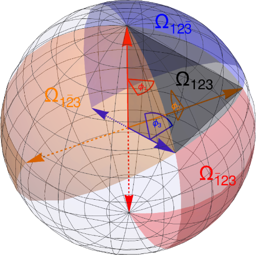
Figure 3: Visualization of the geometrical quantities appearing in the result (72) for the massless integral in six dimensions. Analogous to figure 2, the picture shows the slice $x_{0}=1$ of six-dimensional Minkowski space, specifically the three-dimensional subspace defined by $\vec{v}_{1}$, $\vec{v}_{2}$, $\vec{v}_{3}$. These vectors span a tetrahedron with volume $\mathbb{V}(\vec{v}_{1},\vec{v}_{2},\vec{v}_{3})$ shaded in gray. Note that the factor of $6$ in eq. (72) is not from $d=6$ but originates from eq. (34). The dihedral angle between the faces that meet at $\vec{v}_{i}$ is denoted by $\phi_{i}$, i.e. e.g. $\phi_{1}$ is the angle between the face spanned by $(\vec{v}_{1},\vec{v}_{2})$ and $(\vec{v}_{1},\vec{v}_{3})$. They contribute with $\mathrm{Cl}_{2}(2\phi_{i})$ in eq. (72). The $\Omega$ are solid angles, i.e. areas of triangles on the the unit sphere. The red area $\Omega_{\bar{1}23}$ has corners at $(-\vec{v}_{1},\vec{v}_{2},\vec{v}_{3})$, the yellow area $\Omega_{1\bar{2}3}$ has corners at $(\vec{v}_{1},-\vec{v}_{2},\vec{v}_{3})$, and the blue area $\Omega_{\bar{1}23}$ has corners at $(\vec{v}_{1},\vec{v}_{2},-\vec{v}_{3})$. They contribute with $\mathrm{Cl}_{2}(\Omega)$ in eq. (72). The black area $\Omega_{123}$ is the solid angle covered by $(\vec{v}_{1},\vec{v}_{2},\vec{v}_{3})$ and contributes negatively with $-\mathrm{Cl}_{2}(\Omega)$ in eq. (72).

Hence the massless three-denominator angular integral in six dimensions can be presented in the form

$$I_{111}^{(0),d=6}=\frac{\pi}{6\mathbb{V}(\vec{v}_{1},\vec{v}_{2},\vec{v}_{3})}\Big{[}\mathrm{Cl}_{2}(2\phi_{1})+\mathrm{Cl}_{2}(2\phi_{2})+\mathrm{Cl}_{2}(2\phi_{3})+\mathrm{Cl}_{2}(\Omega_{\bar{1}23})+\mathrm{Cl}_{2}(\Omega_{1\bar{2}3})+\mathrm{Cl}_{2}(\Omega_{12\bar{3}})-\mathrm{Cl}_{2}(\Omega_{123})\Big{]},$$ (72)

where the geometric meaning of each object is visualized in figure 3. Curiously, we observe that the Clausen function is related to the volume of hyperbolic tetrahedra (see appendix H), while the arguments in eq. (72) are all given in relation to Euclidean tetrahedra. With dihedral angles, solid angles, and the Clausen function eq. (72) combines quantities from Euclidean, spherical, and hyperbolic geometry.

VIII.2 Single-massive integral

For the single-massive three-denominator integral we find the $\varepsilon$-expansion

$$I_{111}^{(1)}(v_{12},v_{13},v_{23},v_{11};\varepsilon)=-\frac{\pi}{\varepsilon}\frac{(v_{12}+v_{13})}{v_{12}v_{13}v_{23}}$$

$$+\frac{\pi}{v_{12}v_{13}v_{23}(2v_{12}v_{13}-v_{11}v_{23})}\Big{[}v_{13}(v_{11}v_{23}+v_{12}^{2}-v_{12}v_{13}-v_{12}v_{23})\log\frac{v_{11}}{v_{12}^{2}}$$

$$\qquad+v_{12}(v_{11}v_{23}+v_{13}^{2}-v_{12}v_{13}-v_{13}v_{23})\log\frac{v_{11}}{v_{13}^{2}}+2v_{12}v_{13}(v_{12}+v_{13}-v_{23})\log\frac{v_{23}}{2}\Big{]}$$

$$+\frac{2\pi\,\varepsilon}{v_{12}v_{13}v_{23}(2v_{12}v_{13}-v_{11}v_{23})}\left[\vphantom{\frac{\textbullet}{\textbullet}}\right.v_{12}v_{13}(v_{12}+v_{13}-v_{23})\,\mathrm{Li}_{2}\!\left(1-\frac{2}{v_{23}}\right)$$

$$\qquad+v_{13}(v_{11}v_{23}+v_{12}^{2}-v_{12}v_{13}-v_{12}v_{23})\left(\mathrm{Li}_{2}\!\left(1-\frac{v_{12}}{1+\sqrt{1-v_{11}}}\right)+\mathrm{Li}_{2}\!\left(1-\frac{v_{12}}{1-\sqrt{1-v_{11}}}\right)+\frac{1}{4}\log\frac{v_{11}}{v_{12}^{2}}\right)$$

$$\qquad+v_{12}(v_{11}v_{23}+v_{13}^{2}-v_{12}v_{13}-v_{13}v_{23})\left(\mathrm{Li}_{2}\!\left(1-\frac{v_{13}}{1+\sqrt{1-v_{11}}}\right)+\mathrm{Li}_{2}\!\left(1-\frac{v_{13}}{1-\sqrt{1-v_{11}}}\right)+\frac{1}{4}\log\frac{v_{11}}{v_{13}^{2}}\right)$$

$$\qquad+v_{12}v_{13}\sqrt{Y_{123}^{(1)}}f_{Y}^{(1)}(v_{12},v_{13},v_{23},v_{11})\left.\vphantom{\frac{}{}}\right],$$ (73)

where

$$f_{Y}^{(1)} (v_{12},v_{13},v_{23},v_{11})=\frac{\sqrt{Y_{123}^{(1)}}}{\pi}I_{111}^{(1),d=6}=\frac{J_{111}^{(1)}(-1)}{\pi}=f_{Y}^{(0)}+\int_{0}^{v_{11}}\mathrm{d}v\,j^{(1)}(v)$$

$$= \,\mathrm{Cl}_{2}\!\left(2\theta_{1}^{(0)}\right)+\mathrm{Cl}_{2}\!\left(2\theta_{2}^{(1)}\right)+\mathrm{Cl}_{2}\!\left(2\theta_{3}^{(1)}\right)+\mathrm{Cl}_{2}\!\left(2\theta_{12}^{(0)}\right)+\mathrm{Cl}_{2}\!\left(2\theta_{13}^{(0)}\right)+2\mathrm{Cl}_{2}\!\left(2\theta_{23}^{(1)}\right)-\mathrm{Cl}_{2}\!\left(2\theta_{23}^{(0)}\right)-\mathrm{Cl}_{2}\!\left(2\theta_{123}^{(0)}\right)$$

$$+\frac{1}{2}\mathrm{Cl}_{2}\!\left(2\theta_{2}^{(1)}+2\theta_{2}^{(0)}\right)+\frac{1}{2}\mathrm{Cl}_{2}\!\left(2\theta_{2}^{(1)}-2\theta_{2}^{(0)}\right)-\frac{1}{2}\mathrm{Cl}_{2}\!\left(4\theta_{2}^{(1)}\right)$$

$$+\frac{1}{2}\mathrm{Cl}_{2}\!\left(2\theta_{3}^{(1)}+2\theta_{3}^{(0)}\right)+\frac{1}{2}\mathrm{Cl}_{2}\!\left(2\theta_{3}^{(1)}-2\theta_{3}^{(0)}\right)-\frac{1}{2}\mathrm{Cl}_{2}\!\left(4\theta_{3}^{(1)}\right)$$

$$+\mathrm{Cl}_{2}\!\left(2\theta_{23}^{(1)}+2\theta_{23}^{(0)}\right)+\mathrm{Cl}_{2}\!\left(2\theta_{23}^{(1)}-2\theta_{23}^{(0)}\right)-\mathrm{Cl}_{2}\!\left(4\theta_{23}^{(1)}\right)$$

$$+\frac{1}{2}\mathrm{Cl}_{2}\!\left(2\phi_{12,+}^{(1)}+2\phi_{12,+}^{(0)}\right)+\frac{1}{2}\mathrm{Cl}_{2}\!\left(2\phi_{12,+}^{(1)}-2\phi_{12,+}^{(0)}\right)+\frac{1}{2}\mathrm{Cl}_{2}\!\left(2\phi_{12,-}^{(1)}+2\phi_{12,-}^{(0)}\right)+\frac{1}{2}\mathrm{Cl}_{2}\!\left(2\phi_{12,-}^{(1)}-2\phi_{12,-}^{(0)}\right)$$

$$-\frac{1}{2}\mathrm{Cl}_{2}\!\left(2\phi_{12,+}^{(1)}+2\phi_{12,-}^{(0)}\right)-\frac{1}{2}\mathrm{Cl}_{2}\!\left(2\phi_{12,+}^{(1)}-2\phi_{12,-}^{(0)}\right)-\frac{1}{2}\mathrm{Cl}_{2}\!\left(2\phi_{12,-}^{(1)}+2\phi_{2,+}^{(0)}\right)-\frac{1}{2}\mathrm{Cl}_{2}\!\left(2\phi_{12,-}^{(1)}-2\phi_{12,+}^{(0)}\right)$$

$$+\mathrm{Cl}_{2}\!\left(2\phi_{12,+}^{(0)}+2\phi_{12,-}^{(0)}\right)-\frac{1}{2}\mathrm{Cl}_{2}\!\left(4\phi_{12,+}^{(0)}\right)-\frac{1}{2}\mathrm{Cl}_{2}\!\left(4\phi_{12,-}^{(0)}\right)$$

$$+\frac{1}{2}\mathrm{Cl}_{2}\!\left(2\phi_{13,+}^{(0)}+2\phi_{13,+}^{(1)}\right)+\frac{1}{2}\mathrm{Cl}_{2}\!\left(2\phi_{13,+}^{(1)}-2\phi_{13,+}^{(0)}\right)+\frac{1}{2}\mathrm{Cl}_{2}\!\left(2\phi_{13,-}^{(1)}+2\phi_{13,-}^{(0)}\right)+\frac{1}{2}\mathrm{Cl}_{2}\!\left(2\phi_{13,-}^{(1)}-2\phi_{13,-}^{(0)}\right)$$

$$-\frac{1}{2}\mathrm{Cl}_{2}\!\left(2\phi_{13,+}^{(1)}+2\phi_{13,-}^{(0)}\right)-\frac{1}{2}\mathrm{Cl}_{2}\!\left(2\phi_{13,+}^{(1)}-2\phi_{13,-}^{(0)}\right)-\frac{1}{2}\mathrm{Cl}_{2}\!\left(2\phi_{13,-}^{(1)}+2\phi_{13,+}^{(0)}\right)-\frac{1}{2}\mathrm{Cl}_{2}\!\left(2\phi_{13,-}^{(1)}-2\phi_{13,+}^{(0)}\right)$$

$$+\mathrm{Cl}_{2}\!\left(2\phi_{13,+}^{(0)}+2\phi_{13,-}^{(0)}\right)-\frac{1}{2}\mathrm{Cl}_{2}\!\left(4\phi_{13,+}^{(0)}\right)-\frac{1}{2}\mathrm{Cl}_{2}\!\left(4\phi_{13,-}^{(0)}\right),$$ (74)

with the abbreviations from (68) and

$$\phi_{1j,\pm}^{(0)} =\arctan\!\left(\frac{\sqrt{Y_{123}^{(0)}}}{v_{1j}+v_{jk}-v_{1k}-v_{1j}v_{jk}}\,\frac{1-v_{1j}+\sqrt{1-w_{jk}}}{1\pm\sqrt{1-w_{jk}}}\right),$$ (75)

$$\phi_{1j,\pm}^{(1)} =\arctan\!\left(\frac{\sqrt{Y_{123}^{(1)}}}{v_{1j}+v_{jk}-v_{1k}-v_{1j}v_{jk}}\,\frac{1-v_{1j}+\sqrt{1-w_{jk}}}{\sqrt{1-v_{11}}\pm\sqrt{1-w_{jk}}}\right),$$ (76)

where ${j,k}\in\{2,3\}$ with $j\neq k$ and

$$w_{jk}=\frac{Y_{123}^{(0)}}{v_{jk}(2-v_{jk})}\,.$$ (77)

The quantities $Y_{123}^{(0,1)}$ are given in eqs. (39) respectively (40). As in the massless case, the result simplifies to a sum of two-denominator integrals in the case where the vectors $\vec{v}_{1,2,3}$ become linearly dependent. The pole part is identical to the result found in [7], while the finite part agrees in the limit of small mass $v_{11}$ with the result calculated in [7] via expansion by regions.

VIII.3 Double- and triple-massive integral

The $\varepsilon$-expansions of the double- and triple-massive integral could be obtained by plugging the massless and single-massive results from eqs.(66) and (73) into eqs.(14) and (15). However, it is much more economical to first use eq. (24) to extract the part that is expressible in terms of known two-denominator integrals. Subsequently eqs.(14) and (15) need to be applied only to $I_{111}^{d=6}$. By absorbing a factor of $\sqrt{Y_{123}}$, we can apply the mass splitting in the form of (21) respectively (22). Therefore the order $\varepsilon$ term in the double- respectively triple-massive case is conveniently expressed in terms of the functions

$$f_{Y}^{(2)}(v_{12},v_{13},v_{23},v_{11},v_{22})=f_{Y}^{(0)}\left(v_{3(12)},v_{3(21)},v_{(12)(21)}\right)-f_{Y}^{(1)}\left(v_{13},v_{1(12)},v_{3(12)},v_{11}\right)-f_{Y}^{(1)}\left(v_{23},v_{2(21)},v_{3(21)},v_{22}\right),$$ (78)

respectively

$$f_{Y}^{(3)} (v_{12},v_{13},v_{23},v_{11},v_{22},v_{33})=f_{Y}^{(1)}\left(v_{3(12)},v_{3(21)},v_{(12)(21)},v_{33}\right)-f_{Y}^{(0)}\left(v_{(12)(13)},v_{(12)(31)},v_{(13)(31)}\right)$$

$$+f_{Y}^{(1)}\left(v_{1(12)},v_{1(13)},v_{(12)(13)},v_{11}\right)+f_{Y}^{(1)}\left(v_{3(12)},v_{3(31)},v_{(12)(31)},v_{33}\right)-f_{Y}^{(0)}\left(v_{(21)(23)},v_{(21)(32)},v_{(23)(32)}\right)$$

$$+f_{Y}^{(1)}\left(v_{2(21)},v_{2(23)},v_{(21)(23)},v_{22}\right)+f_{Y}^{(1)}\left(v_{3(21)},v_{3(32)},v_{(21)(32)},v_{33}\right).$$ (79)

The necessary massless and single-massive functions $f_{Y}^{(0)}$ and $f_{Y}^{(1)}$ are given in eqs. (67) and (74). For compact notation we introduce the further functions

$$f_{1}^{(0)}(v_{ij}) \equiv 2\,\mathrm{Li}_{2}\!\left(1-\frac{2}{v_{ij}}\right),$$ (80)

$$f_{1}^{(1)}(v_{ij},v_{ii}) \equiv-2\,\mathrm{Li}_{2}\!\left(1-\frac{v_{ij}}{1+\sqrt{1-v_{ii}}}\right)-2\mathrm{Li}_{2}\!\left(1-\frac{v_{ij}}{1-\sqrt{1-v_{ii}}}\right)-\frac{1}{2}\log^{2}\!\left(\frac{v_{ii}}{v_{ij}^{2}}\right),$$ (81)

$$f_{1}^{(2)}(v_{ij},v_{ii},v_{jj}) \equiv f_{1}^{(0)}(v_{(ij)(ji)})-f_{1}^{(1)}(v_{i(ij)},v_{ii})-f_{1}^{(1)}(v_{j(ji)},v_{jj})\,.$$ (82)

With these abbreviations in place, the $\varepsilon$-expansion of the double-massive three-denominator integral is given by

$$I_{111}^{(2)} (v_{12},v_{13},v_{23},v_{11},v_{22};\varepsilon)=-\frac{\pi}{\varepsilon}\frac{1}{v_{13}v_{23}}+\frac{\pi}{2v_{12}v_{23}v_{13}-v_{11}v_{23}^{2}-v_{22}v_{13}^{2}}$$

$$\times\left[\Big{(}v_{13}-v_{12}-v_{23}+\frac{v_{11}v_{23}}{v_{13}}\Big{)}\log\frac{v_{11}}{v_{13}^{2}}\right.+\Big{(}v_{23}-v_{12}-v_{13}+\frac{v_{22}v_{13}}{v_{23}}\Big{)}\log\frac{v_{22}}{v_{23}^{2}}$$

$$\left.\qquad+\frac{1}{\sqrt{X_{12}}}\Big{(}v_{12}\left(v_{13}+v_{23}-v_{12}\right)-v_{11}v_{23}-v_{22}v_{13}+v_{11}v_{22}\Big{)}\log\!\left(\frac{v_{12}+\sqrt{X_{12}}}{v_{12}-\sqrt{X_{12}}}\right)\right]$$

$$+\frac{\pi}{2v_{12}v_{23}v_{13}-v_{11}v_{23}^{2}-v_{22}v_{13}^{2}}\left[\frac{1}{\sqrt{X_{12}}}\Big{(}v_{12}\left(v_{13}+v_{23}-v_{12}\right)-v_{11}v_{23}-v_{22}v_{13}+v_{11}v_{22}\Big{)}f_{1}^{(2)}(v_{12},v_{11},v_{22})\right.$$

$$\qquad-\Big{(}v_{13}-v_{12}-v_{23}+\frac{v_{11}v_{23}}{v_{13}}\Big{)}f_{1}^{(1)}(v_{13},v_{11})-\Big{(}v_{23}-v_{12}-v_{13}+\frac{v_{22}v_{13}}{v_{23}}\Big{)}f_{1}^{(1)}(v_{23},v_{22})$$

$$\left.\qquad+2\sqrt{Y_{123}^{(2)}}\,f_{Y}^{(2)}(v_{12},v_{13},v_{23},v_{11},v_{22})\right]+\mathcal{O}\!\left(\varepsilon^{2}\right)\,.$$ (83)

with $f_{Y}^{(2)}$ from eq. (78). Finally, using the kinematic quantities from section IV, the triple-massive three-denominator integral has the $\varepsilon$-expansion

$$I_{111}^{(3)} =\frac{\pi}{X_{123}^{(3)}}\left[\frac{X_{12\bar{3}}}{\sqrt{X_{12}}}\log\!\left(\frac{v_{12}+\sqrt{X_{12}}}{v_{12}-\sqrt{X_{12}}}\right)+\frac{X_{1\bar{2}3}}{\sqrt{X_{13}}}\log\!\left(\frac{v_{13}+\sqrt{X_{13}}}{v_{13}-\sqrt{X_{13}}}\right)+\frac{X_{\bar{1}23}}{\sqrt{X_{23}}}\log\!\left(\frac{v_{23}+\sqrt{X_{23}}}{v_{23}-\sqrt{X_{23}}}\right)\right]$$

$$+\frac{\pi\,\varepsilon}{X_{123}^{(3)}}\left[\frac{X_{12\bar{3}}}{\sqrt{X_{12}}}f_{1}^{(2)}(v_{12},v_{11},v_{22})+\frac{X_{1\bar{2}3}}{\sqrt{X_{13}}}f_{1}^{(2)}(v_{13},v_{11},v_{33})+\frac{X_{\bar{1}23}}{\sqrt{X_{23}}}f_{1}^{(2)}(v_{23},v_{22},v_{33})+2\sqrt{Y_{123}^{(3)}}\,f_{Y}^{(3)}\right]+\mathcal{O}\!\left(\varepsilon^{2}\right)$$ (84)

with $f_{Y}^{(3)}$ from eq. (79). For the double- and triple-massive integral, poles and small-mass limit of the finite part are also in agreement with the results from [7].

IX Beyond three denominators

If we consider a situation in $d=4-2\varepsilon$ dimensions where all vectors $v_{i}$ are confined to the physical $4$-dimensional subspace – an assumption applicable if the $v_{i}$ correspond to momenta of observed particles – we can reduce angular integrals with an arbitrary number of denominators raised to integer powers to the three-denominator case presented in this paper. This is possible since in $4$ dimensions, i.e. three spatial dimensions, no more than three $\vec{v}_{i}$ can be linearly dependent. Hence for any $n>3$ and vectors $v_{1},\dots,v_{n}$ there are constants $\lambda_{i}$ such that $\lambda\equiv\sum_{i=1}^{n}\lambda_{i}\neq 0$ but $0=\sum_{i=1}^{n}\lambda_{i}\vec{v}_{i}$. By partial fractioning it holds that [5]

$$\prod_{i=1}^{n}\frac{1}{v_{i}\cdot k}=\frac{1}{\lambda}\sum_{j=1}^{n}\lambda_{j}\prod_{\overset{i=1}{i\neq j}}^{n}\frac{1}{v_{i}\cdot k}\,,$$ (85)

which reduces the number of denominators in each term. Iterative application of this identity reduces any $I_{j_{1},\dots,j_{n}}$ with integer-valued $j_{i}$ to the three-denominator case. Therefore the presented results can be applied to this much wider class of angular integrals.

X Conclusion

In this work we performed the first systematic study of angular integrals with three denominators and an arbitrary number of masses. From IBP relations we derived explicit recursion relations for the reduction to a small set of master integrals. The $\varepsilon$-expansion of the master integrals was calculated using the method of differential equations.

This methodology, which is well established for loop integrals, was combined with a dimensional-shift identity for angular integrals which allows for an extraction of the pole part before calculating the integral. In the case of three denominators the order $\varepsilon^{0}$ also turns out to be fully determined by two-denominator integrals, the unknown genuine three-denominator part only starts contributing at order $\varepsilon$. The remaining non-trivial part at order $\varepsilon$, which contributes proportional to a Euclidean Gram determinant, has been expressed in terms of Clausen functions. In the massless case we were able to give a geometrical interpretation of all involved quantities. The ancillary Mathematica file provides the function AngularIntegral[{j1_,j2_,j3_},{v12_,v13_,v23_,v11_,v22_,v33_}] which evaluates the three-denominator angular integral in $d=4-2\varepsilon$ dimensions up to order $\varepsilon$.

In parallel work, Taushif Ahmed, Syed Mehedi Hasan, and Andreas Rapakoulias independently calculated the angular integral with three denominators using Mellin-Barnes integrals [52]. Preliminary numerical comparison at selected phase space points showed agreement.

Appendix A Scalar products for mass reduction formula

The scalar products involving the massless auxiliary vectors appearing in section III are given by ($i,j,k\in\{1,2,3\}$)

$$v_{i(ij)} =\frac{X_{ij}+(v_{ii}-v_{ij})\sqrt{X_{ij}}}{2v_{ij}-v_{ii}-v_{jj}}\,,$$ (86)

$$v_{(ij)(ji)} =\frac{2X_{ij}}{2v_{ij}-v_{ii}-v_{jj}}\,,$$ (87)

$$v_{k(ij)} =\frac{v_{ij}v_{jk}-v_{ik}v_{jj}+v_{ij}v_{ik}-v_{ii}v_{jk}+(v_{ik}-v_{jk})\sqrt{X_{ij}}}{2v_{ij}-v_{ii}-v_{jj}}\,,$$ (88)

$$v_{(ij)(ik)} =\frac{1}{(2v_{ij}-v_{ii}-v_{jj})(2v_{ik}-v_{ii}-v_{kk})}\Big{[}v_{ii}^{2}v_{jk}-v_{ii}v_{ij}v_{ik}-v_{ii}v_{ij}v_{jk}-v_{ii}v_{ik}v_{jk}+v_{ii}v_{jj}v_{kk}+v_{ij}v_{ik}^{2}$$

$$\qquad+v_{ij}^{2}v_{ik}-v_{jj}v_{ik}^{2}+v_{ij}v_{ik}v_{jk}-v_{kk}v_{ij}^{2}-\sqrt{X_{ij}}\left(v_{ij}v_{ik}+v_{ik}v_{jk}-v_{ii}v_{jk}-v_{kk}v_{ij}-v_{ik}^{2}+v_{ii}v_{kk}\right)$$

$$\qquad-\sqrt{X_{ik}}\left(v_{ij}v_{ik}+v_{ij}v_{jk}-v_{jj}v_{ik}-v_{ii}v_{jk}-v_{ij}^{2}+v_{ii}v_{jj}\right)+\left(-v_{ij}-v_{ik}+v_{ii}+v_{jk}\right)\sqrt{X_{ij}X_{ik}}\Big{]}\,,$$ (89)

$$v_{(ij)(ki)} =\frac{1}{(2v_{ij}-v_{ii}-v_{jj})(2v_{ik}-v_{ii}-v_{kk})}\Big{[}v_{ii}^{2}v_{jk}-v_{ii}v_{ij}v_{ik}-v_{ii}v_{ij}v_{jk}-v_{ii}v_{ik}v_{jk}+v_{ii}v_{jj}v_{kk}+v_{ij}v_{ik}^{2}$$

$$\qquad+v_{ij}^{2}v_{ik}-v_{jj}v_{ik}^{2}+v_{ij}v_{ik}v_{jk}-v_{kk}v_{ij}^{2}-\sqrt{X_{ij}}\left(v_{ij}v_{ik}+v_{ik}v_{jk}-v_{ii}v_{jk}-v_{kk}v_{ij}-v_{ik}^{2}+v_{ii}v_{kk}\right)$$

$$\qquad-\sqrt{X_{ik}}\left(-v_{ij}v_{ik}-v_{ij}v_{jk}+v_{jj}v_{ik}+v_{ii}v_{jk}+v_{ij}^{2}-v_{ii}v_{jj}\right)+\left(v_{ij}+v_{ik}-v_{ii}-v_{jk}\right)\sqrt{X_{ij}X_{ik}}\Big{]}\,,$$ (90)

where $X_{ij}=v_{ij}^{2}-v_{ii}v_{jj}$ .

Appendix B Full form of IBP relations

Plugging the six different $\vec{\xi}$ given in eqs. (4) and (5) into eq.(8) we obtain the following set of IBP relations:

$$\text{for }\vec{\xi}_{1k}\text{: }0= \left(-d+j_{1}+j_{2}+j_{3}+2\right)I_{j_{1}-1,j_{2},j_{3}}+\left(d-2j_{1}-j_{2}-j_{3}-2\right)I_{j_{1},j_{2},j_{3}}+j_{3}\,v_{13}\,I_{j_{1},j_{2},j_{3}+1}$$

$$+j_{2}\,v_{12}\,I_{j_{1},j_{2}+1,j_{3}}+j_{1}\,v_{11}\,I_{j_{1}+1,j_{2},j_{3}}-j_{3}\,I_{j_{1}-1,j_{2},j_{3}+1}-j_{2}\,I_{j_{1}-1,j_{2}+1,j_{3}}\,,$$ (91)

$$\text{for }\vec{\xi}_{12}\text{: }0= j_{3}\left(v_{23}-1\right)I_{j_{1}-1,j_{2},j_{3}+1}+j_{2}\left(v_{22}-1\right)I_{j_{1}-1,j_{2}+1,j_{3}}-j_{3}\left(v_{13}-1\right)I_{j_{1},j_{2}-1,j_{3}+1}$$

$$+\left(j_{1}-j_{2}\right)\left(v_{12}-1\right)I_{j_{1},j_{2},j_{3}}+j_{3}\left(v_{13}-v_{23}\right)I_{j_{1},j_{2},j_{3}+1}+j_{2}\left(v_{12}-v_{22}\right)I_{j_{1},j_{2}+1,j_{3}}$$

$$-j_{1}\left(v_{11}-1\right)I_{j_{1}+1,j_{2}-1,j_{3}}+j_{1}\left(v_{11}-v_{12}\right)I_{j_{1}+1,j_{2},j_{3}}$$ (92)

IBP relations for $\xi_{2k}$, $\xi_{3k}$, $\xi_{13}$, and $\xi_{23}$ follow by appropriate permutation of indices.

Appendix C Recursion relations for three-denominator angular integrals

By taking suitable linear combinations, the IBP relations can be cast into explicit recursions. A recursion relation that lowers the sum of indices $j=j_{1}+j_{2}+j_{3}$, applicable for $j_{1}\neq 1$, is given by

$$I_{j_{1},j_{2},j_{3}}=\frac{1}{(1-j_{1})X_{123}}\Big{[} -\left(v_{23}^{2}-v_{22}v_{33}\right)\left(-d+j+1\right)I_{j_{1}-2,j_{2},j_{3}}+\left(v_{13}v_{23}-v_{12}v_{33}\right)\left(-d+j+1\right)I_{j_{1}-1,j_{2}-1,j_{3}}$$

$$-\left(v_{13}v_{22}-v_{12}v_{23}\right)\left(-d+j+1\right)I_{j_{1}-1,j_{2},j_{3}-1}+[(v_{12}v_{23}-v_{13}v_{22})(d-j_{1}-j_{2}-2j_{3}-1)$$

$$+(v_{13}v_{23}-v_{12}v_{33})(d-j_{1}-2j_{2}-j_{3}-1)+\left(v_{22}v_{33}-v_{23}^{2}\right)(d-2j_{1}-j_{2}-j_{3})]I_{j_{1}-1,j_{2},j_{3}}$$

$$+j_{3}\left(v_{23}^{2}-v_{22}v_{33}\right)I_{j_{1}-2,j_{2},j_{3}+1}+j_{2}\left(v_{23}^{2}-v_{22}v_{33}\right)I_{j_{1}-2,j_{2}+1,j_{3}}$$

$$+j_{3}\left(v_{12}v_{33}-v_{13}v_{23}\right)I_{j_{1}-1,j_{2}-1,j_{3}+1}+j_{2}\left(v_{13}v_{22}-v_{12}v_{23}\right)I_{j_{1}-1,j_{2}+1,j_{3}-1}$$

$$+\left(j_{1}-1\right)\left(v_{12}v_{33}-v_{13}v_{23}\right)I_{j_{1},j_{2}-1,j_{3}}+\left(j_{1}-1\right)\left(v_{13}v_{22}-v_{12}v_{23}\right)I_{j_{1},j_{2},j_{3}-1}\Big{]},$$ (93)

where $X_{123}$ is the Gram determinant defined in section IV.

There are also the symmetric identities with $1\leftrightarrow 2$ and $1\leftrightarrow 3$ applicable for $j_{2,3}\neq 1$. These identities allow for a systematic reduction of any $I_{j_{1},j_{2},j_{3}}$ with $j_{1},j_{2},j_{3}>0$ to the case where either $j_{1}=j_{2}=j_{3}=1$ or one of the indices becomes $0$. From there, recursion relations for two denominators can be used for further reduction [5]. To deal with integrals with a negative index, we can use

$$I_{j_{1},j_{2},j_{3}}= \frac{1}{(3+j-d)Y_{23}}\Big{[}[v_{23}^{2}\left(-d+2j_{1}+j_{2}+j_{3}+4\right)$$

$$\qquad+v_{23}\left(j_{2}\left(v_{12}-3\right)+\left(j_{3}-1\right)v_{13}-j_{1}\left(v_{12}+v_{13}+2\right)-v_{12}+2d-3j_{3}-6\right)$$

$$\qquad+v_{33}\left(\left(j_{1}-j_{2}+1\right)v_{12}-d+j_{1}+2j_{2}+j_{3}+3\right)$$

$$\qquad+v_{22}\left(d\left(v_{33}-1\right)+j_{1}v_{13}-j_{3}v_{13}-\left(2j_{1}+j_{2}+j_{3}+4\right)v_{33}+v_{13}+j_{1}+j_{2}+2j_{3}+3\right)]I_{j_{1}+1,j_{2},j_{3}}$$

$$+j_{3}\left(v_{13}-1\right)\left(v_{23}-v_{33}\right)I_{j_{1}+1,j_{2}-1,j_{3}+1}-j_{3}\left(v_{13}-1\right)\left(v_{23}^{2}-v_{22}v_{33}\right)I_{j_{1}+1,j_{2},j_{3}+1}$$

$$-j_{2}\left(v_{12}-1\right)\left(v_{22}-v_{23}\right)I_{j_{1}+1,j_{2}+1,j_{3}-1}-j_{2}\left(v_{12}-1\right)\left(v_{23}^{2}-v_{22}v_{33}\right)I_{j_{1}+1,j_{2}+1,j_{3}}$$

$$+\left(j_{1}+1\right)\left(v_{11}-1\right)\left(v_{23}-v_{33}\right)I_{j_{1}+2,j_{2}-1,j_{3}}-\left(j_{1}+1\right)\left(v_{11}-1\right)\left(v_{22}-v_{23}\right)I_{j_{1}+2,j_{2},j_{3}-1}$$

$$-\left(j_{1}+1\right)\left(v_{13}\left(v_{22}-v_{23}\right)+v_{12}\left(v_{33}-v_{23}\right)+v_{11}\left(v_{23}^{2}-v_{22}v_{33}\right)\right)I_{j_{1}+2,j_{2},j_{3}}\Big{]},$$ (94)

where

$$Y_{23}=(\vec{v}_{2}\cdot\vec{v}_{3})^{2}-\vec{v}_{2}^{2}\,\vec{v}_{3}^{2}=v_{22}+v_{33}-v_{22}v_{33}-v_{23}(2-v_{23})\,,$$ (95)

which raises $j_{1}+j_{2}+j_{3}$ as well as $j_{1}$. Again there are the symmetric versions that raise $j_{2}$ respectively $j_{3}$. These can be used to increase any negative index to $0$ again resulting in two-denominator integrals. We note that $Y_{23}$ has the geometrical interpretation $Y_{23}=4\mathbb{V}^{2}(\vec{v}_{2},\vec{v}_{3})$, where $\mathbb{V}(\vec{v}_{2},\vec{v}_{3})$ denotes the area of the triangle spanned by $\vec{v}_{2,3}$.

Appendix D Proof of the general dimensional-shift identity

In this appendix we prove the general dimensional-shift identity eq. (23). The proof is a straightforward generalization of the two-denominator case given in [5]. We start from the hypergeometric representation of the one-denominator angular integral in $d=4-2\varepsilon$ dimensions,

$$I^{(1)}_{j}(v^{2};\varepsilon)=\frac{2\pi}{1-2\varepsilon}\,{}_{2}\mathrm{F}_{1}\!\left(\frac{j}{2},\frac{j+1}{2},\frac{3}{2}-\varepsilon;1-v^{2}\right).$$ (96)

Using the contiguous neighbors relation

$${}_{2}\mathrm{F}_{1}(a,b,c-1;z)=\frac{1}{c-1}\Big{[}a\,{}_{2}\mathrm{F}_{1}(a+1,b,c;z)+(c-1-a)\,{}_{2}\mathrm{F}_{1}(a,b,c;z)\Big{]},$$ (97)

and the symmetry of the hypergeometric function in its first two arguments we can identify the hypergeometric functions with one-denominator integrals with $\varepsilon\rightarrow\varepsilon-1$,

$$I^{(1)}_{j}(v^{2};\varepsilon)=\frac{1}{1-2\varepsilon}\left[j\,I^{(1)}_{j+1}(v^{2};\varepsilon-1)+(3-j-2\varepsilon)\,I^{(1)}_{j}(v^{2};\varepsilon-1)\right]\,.$$ (98)

Now considering the general case of $n$ denominators, we use a Feynman parametrization of the denominator and obtain

$$I_{j_{1}\dots j_{n}} =\int\frac{\mathrm{d}\Omega_{d-1}}{\Omega_{d-3}}\frac{1}{(v_{1}\cdot k)^{j_{1}}\cdots(v_{n}\cdot k)^{j_{n}}}\,$$

$$=\frac{\Gamma(j)}{\Gamma(j_{1})\cdots\Gamma(j_{n})}\int_{0}^{1}\mathrm{d}x_{1}\cdots\int_{0}^{1}\mathrm{d}x_{n}\,x_{1}^{j_{1}}\cdots x_{n}^{j_{n}}\int\frac{\mathrm{d}\Omega_{d-1}}{\Omega_{d-3}}\frac{\delta\!\left(1-\sum_{i=1}^{n}x_{i}\right)}{\left(\sum_{i=1}^{n}x_{i}v_{i}\cdot k\right)^{j}}$$

$$=\frac{\Gamma(j)}{\Gamma(j_{1})\cdots\Gamma(j_{n})}\int_{0}^{1}\mathrm{d}x_{1}\cdots\int_{0}^{1}\mathrm{d}x_{n}\,x_{1}^{j_{1}}\cdots x_{n}^{j_{n}}\,\delta\!\left(1-\sum_{i=1}^{n}x_{i}\right)I_{j}^{(1)}\!\left(\left(\sum_{i=1}^{n}x_{i}v_{i}\right)^{2};\varepsilon\right),$$ (99)

where $j=\sum_{i=1}^{n}j_{i}$. Plugging in eq. (98), the second summand can be directly identified with an $n$-denominator angular integral with $\varepsilon\rightarrow\varepsilon-1$. For the first summand, realizing that

$$x_{1}^{j_{1}}\cdots x_{n}^{j_{n}}\,\delta\!\left(1-\sum_{i=1}^{n}x_{i}\right)=\left[x_{1}^{j_{1}+1}x_{2}^{j_{2}}\cdots x_{n}^{j_{n}}+x_{1}^{j_{1}}x_{2}^{j_{2}+1}\cdots x_{n}^{j_{n}}+x_{1}^{j_{1}}x_{2}^{j_{2}}\cdots x_{n}^{j_{n}+1}\right]\delta\!\left(1-\sum_{i=1}^{n}x_{i}\right),$$ (100)

we achieve $j\rightarrow j+1$ in the Feynman parameters and can thus identify each term with an $n$-denominator angular integral with $\varepsilon\rightarrow\varepsilon-1$ resulting in

$$I_{j_{1},...,j_{n}}(\varepsilon)= \frac{1}{1-2\varepsilon}\left[\sum_{i=1}^{n}j_{i}I_{j_{1},...,j_{i}+1,...,j_{n}}(\varepsilon-1)+\,\left(3-\sum_{i=1}^{n}j_{i}-2\varepsilon\right)I_{j_{1},...,j_{n}}(\varepsilon-1)\right],$$ (101)

which is eq. (23) from the main text.

Appendix E Expansion of dimensionally-shifted two-denominator integrals

In this appendix we list the $\varepsilon$-expansions of the dimensionally-shifted two-denominator integrals used in the differential equation in section VII. They are constructed from the known expansion in $d=4-2\varepsilon$ dimensions [3, 4, 5] via the identities

$$I^{(0)}(\varepsilon-1) =\frac{1-2\varepsilon}{3-2\varepsilon}\,I^{(0)}(\varepsilon)\,,$$ (102)

$$I^{(1)}_{1}(v_{11};\varepsilon-1) =\frac{1-2\varepsilon}{2(1-\varepsilon)(1-v_{11}}\Big{[}I^{(0)}(\varepsilon)-v_{11}\,I^{(1)}_{1}(v_{11};\varepsilon)\Big{]}\,,$$ (103)

$$I^{(0)}_{1,1}(v_{12};\varepsilon-1) =-\frac{1}{2-v_{12}}\left[\frac{1-2\varepsilon}{2\varepsilon}\,I^{(0)}(\varepsilon)+v_{12}\,I^{(0)}_{1,1}(v_{12};\varepsilon)\right],$$ (104)

$$I^{(1)}_{1,1}(v_{12},v_{11};\varepsilon-1) =-\frac{v_{12}}{v_{12}(2-v_{12})-v_{11}}\left[\frac{1-2\varepsilon}{2\varepsilon}\,I^{(0)}(\varepsilon)-\left(1-\frac{v_{11}}{v_{12}}\right)I^{(1)}_{1}(v_{11};\varepsilon)+v_{12}\,I^{(1)}_{1,1}(v_{12},v_{11};\varepsilon)\right],$$ (105)

that follow from applying eq. (23) in the cases of zero, one, and two denominators in combination with IBP reduction to master integrals and subsequently solving for the integrals in $d=4-2\varepsilon$ dimensions.

For the massless two-denominator integral, required in the integration of the massless three-denominator integral, we find the expansion

$$I_{1,1}^{(0)}(v_{12},\varepsilon-1)=-\frac{2\pi\log\left(\frac{v_{12}}{2}\right)}{2-v_{12}}+\mathcal{O}(\varepsilon)\,.$$ (106)

For the massive integral we further need the expansions

$$I^{(0)}(\varepsilon-1) =\frac{2\pi}{3}+\mathcal{O}(\varepsilon)\,,$$ (107)

$$I_{2}^{(1)}(v_{11};\varepsilon-1) =-\frac{2\pi}{1-v_{11}}+\frac{\pi\log\!\left(\frac{1+\sqrt{1-v_{11}}}{1-\sqrt{1-v_{11}}}\right)}{\left(1-v_{11}\right){}^{3/2}}+\mathcal{O}(\varepsilon)\,,$$ (108)

$$I_{1,1}^{(1)}(v_{12},v_{11};\varepsilon-1) =\frac{\pi\left(v_{12}-v_{11}\right)\log\!\left(\frac{1+\sqrt{1-v_{11}}}{1-\sqrt{1-v_{11}}}\right)}{\sqrt{1-v_{11}}\left(v_{12}\left(2-v_{12}\right)-v_{11}\right)}+\frac{\pi\,v_{12}\log\frac{v_{11}}{v_{12}^{2}}}{v_{12}\left(2-v_{12}\right)-v_{11}}+\mathcal{O}(\varepsilon)\,.$$ (109)

Appendix F Calculation of the boundary value for the massless master integral

This appendix is dedicated to the calculation of the boundary value used in the massless master integral. The approach is a direct calculation using a string of series, integral, and special function identities successively reducing the complexity of the original integral. This will finally lead us to a remarkably compact result.

The boundary value for $J^{(0),d=6}_{111}$ is calculated at the symmetric point $v_{12}=v_{13}=v_{23}=1$, where the three vectors are in an orthogonal configuration depicted in figure 2. At this point the Euclidean Gram determinant becomes unity and the defining integral representation eq. (1) becomes

$$J^{(0),d=6}_{111}(1,1,1)=I^{(0),d=6}_{111}(1,1,1)=\frac{1}{2}\int_{0}^{\pi}\mathrm{d}\theta_{1}\int_{0}^{\pi}\mathrm{d}\theta_{2}\int_{0}^{\pi}\mathrm{d}\theta_{3}\frac{\sin^{3}\theta_{1}\sin^{2}\theta_{2}\sin\theta_{3}}{(1-\cos\theta)(1-\sin\theta_{1}\cos\theta_{2})(1-\sin\theta_{1}\sin\theta_{2}\cos\theta_{3})}\,.$$ (110)

Expanding the third denominator in a geometric series and integrating the $\theta_{3}$-integrals, using that

$$\int_{0}^{\pi}\mathrm{d}\theta\sin\theta\cos^{n}\theta=\frac{1+(-1)^{n}}{n+1}$$ (111)

vanishes for odd $n$, we get to

$$J^{(0),d=6}_{111}(1,1,1)=\sum_{n=0}^{\infty}\frac{1}{2n+1}\int_{0}^{\pi}\mathrm{d}\theta_{1}\int_{0}^{\pi}\mathrm{d}\theta_{2}\frac{\sin^{3+2n}\theta_{1}\sin^{2+2n}\theta_{2}}{(1-\cos\theta)(1-\sin\theta_{1}\cos\theta_{2})}=\sum_{n=0}^{\infty}\frac{1}{2n+1}\,I_{1,1}^{(0)}(v_{12}=1;\varepsilon=-n-1)\,,$$ (112)

where we could identify the remaining integral with a massless two-denominator angular integral in $6+2n$ dimensions. This integral has been calculated in $d$ dimensions in terms of the Gauss hypergeometric function [2, 4, 5],

$$I_{1,1}^{(0)}(v_{12};\varepsilon)=-\frac{\pi}{\varepsilon}\,{}_{2}\mathrm{F}_{1}\!\left(1,1,1-\varepsilon;1-\frac{v_{12}}{2}\right).$$ (113)

In the specific case at hand we can further use the identity

$${}_{2}\mathrm{F}_{1}\!\left(1,1,c;\frac{1}{2}\right)=(c-1)\left[\psi^{(0)}\!\left(\frac{c}{2}\right)-\psi^{(0)}\!\left(\frac{c}{2}-\frac{1}{2}\right)\right],$$ (114)

reducing the hypergeometric function to digamma functions $\psi^{(0)}(z)\equiv\frac{\mathrm{d}}{\mathrm{d}z}\Gamma(z)$. This allows for the representation

$$I_{1,1}^{(0)}\!\left(\frac{1}{2};-n-1\right)=\frac{\pi}{n+1}\,{}_{2}\mathrm{F}_{1}\left(1,1,2+n;\frac{1}{2}\right)=\pi\left[\psi^{(0)}\!\left(\frac{n}{2}+1\right)-\psi^{(0)}\!\left(\frac{n}{2}+\frac{1}{2}\right)\right].$$ (115)

Putting this into eq. (112) and splitting the sum in even and odd terms we have

$$J^{(0),d=6}_{111}(1,1,1)=\pi\,\sum_{n=0}^{\infty}\frac{1}{4n+1}\left[\psi^{(0)}\!\left(n+1\right)-\psi^{(0)}\!\left(n+\frac{1}{2}\right)\right]+\pi\,\sum_{n=0}^{\infty}\frac{1}{4n+3}\left[\psi^{(0)}\!\left(n+\frac{3}{2}\right)-\psi^{(0)}\!\left(n+1\right)\right].$$ (116)

The digamma function at integer respectively half-integer values evaluates to

$$\psi^{(0)}\!\left(n\right) =H_{n-1}-\gamma_{\text{E}}\,,$$ (117)

$$\psi^{(0)}\!\left(n+\frac{1}{2}\right) =2\,U_{n}-\gamma_{\text{E}}-2\log 2\,,$$ (118)

where $H_{n}\equiv\sum_{k=1}^{n}1/k$ denotes the harmonic numbers and $U_{n}=\sum_{k=1}^{n}1/(2k-1)$ the odd harmonic numbers. Using the identity

$$H_{n}-2\,U_{n}=-2A_{2n}$$ (120)

where $A_{n}=\sum_{k=1}^{n}(-1)^{k+1}/k$ denotes the alternating harmonic series we find

$$\psi^{(0)}\!\left(n+1\right)-\psi^{(0)}\!\left(n+\frac{1}{2}\right) =-2A_{2n}+2\log 2\,,$$ (121)

$$\psi^{(0)}\!\left(n+\frac{3}{2}\right)-\psi^{(0)}\!\left(n+1\right) =2A_{2n+2}-2\log 2\,.$$ (122)

Combining even and odd terms from both sums we have the representation

$$J^{(0),d=6}_{111}(1,1,1)=2\pi\sum_{n=0}^{\infty}\frac{(-1)^{n}}{2n+1}\left(\log 2-A_{n}\right).$$ (123)

Starting from the integral representation

$$\log 2-A_{n}=\int_{0}^{1}\mathrm{d}x\,\frac{(-x)^{n}}{1+x}\,,$$ (124)

substituting $x=\left(\frac{1-t}{1+t}\right)^{2}$, and performing partial integration with respect to $1/(1+t^{2})$ leads to the representation

$$\log 2-A_{n}=4(-1)^{n}(2n+1)\int_{0}^{1}\frac{\mathrm{d}t}{(1+t)^{2}}\left(\frac{1-t}{1+t}\right)^{2n}\,\arctan t\,.$$ (125)

Plugging this into eq. (123) and summing the geometric series we finally obtain

$$J^{(0),d=6}_{111}(1,1,1)=2\pi\,\int_{0}^{1}\frac{\mathrm{d}t}{t}\,\arctan t=2\pi\,\mathrm{Ti}_{2}(1)=2\pi\sum_{n=1}^{\infty}\frac{(-1)^{n+1}}{(2n+1)^{2}}=2\pi\,\mathrm{C}\,,$$ (126)

where $\mathrm{Ti}_{2}$ is the inverse tangent integral and $\mathrm{C}$ is Catalan’s constant.

Appendix G Useful integrals for the calculation of the master integrals

From Lewin’s delightful book [53] we have the following integrals useful for the integration of eqs. (53) and (59),

$$J_{0}(\delta,x) =\int_{0}^{x}\mathrm{d}t\,\frac{\delta}{\delta^{2}+t^{2}}=\arctan\left(\frac{x}{\delta}\right)\,,$$ (127)

$$J_{1}(\alpha,\delta,x) =\int_{-\alpha}^{x}\mathrm{d}t\,\frac{\delta\log|\alpha+t|}{\delta^{2}+t^{2}}=\frac{\theta+\eta}{2}\log\left(\alpha^{2}+\delta^{2}\right)-\frac{1}{2}\mathrm{Cl}_{2}(2\theta+2\eta)-\frac{1}{2}\mathrm{Cl}_{2}(\pi-2\theta)-\frac{1}{2}\mathrm{Cl}_{2}(\pi-2\eta)\,,$$ (128)

$$J_{2}(\beta,\delta,x) =\int_{0}^{x}\mathrm{d}t\,\frac{\delta\log(\beta^{2}+t^{2})}{\delta^{2}+t^{2}}=-\varphi\log\left|\frac{\beta-\delta}{\beta+\delta}\right|+\theta\log|(\beta-\delta)(\beta+\delta)|$$

$$\hphantom{=\int_{0}^{x}\mathrm{d}t\,\frac{\delta\log(\beta^{2}+t^{2})}{\delta^{2}+t^{2}}=}+\frac{1}{2}\mathrm{Cl}_{2}\!\left(2\theta-2\varphi\right)+\frac{1}{2}\mathrm{Cl}_{2}\!\left(2\theta+2\varphi\right)-\mathrm{Cl}_{2}\!\left(2\theta\right),$$ (129)

with the abbreviations

$$\theta=\arctan\frac{x}{\delta}\,,\quad\eta=\arctan\frac{\alpha}{\delta}\,,\quad\varphi=\arctan\frac{x}{\beta}\,.$$ (130)

Here $\mathrm{Cl}_{2}$ denotes the Clausen function recalled in appendix H.

To simplify the arguments of the Clausen functions in these expressions one may use the addition theorem of the arcus tangent

$$\arctan x+\arctan y=\arctan\frac{x+y}{1-xy}+\pi\,\mathrm{sgn}(x+y)\,\Theta(xy-1)\,,$$ (131)

where the $\pi$ term can always be dropped because of the $2\pi$-periodicity of $\mathrm{Cl}_{2}$.

Appendix H Clausen function

The Clausen function $\mathrm{Cl}_{2}(\theta)$, named after 19th century Danish astronomer and mathematician Thomas Clausen, who calculated the function to 16 decimal places in 1832 [54], is defined by the Fourier series

$$\mathrm{Cl}_{2}(\theta)=\sum_{n=1}^{\infty}\frac{\sin(n\theta)}{n^{2}}\,.$$ (132)

It arises naturally by considering the dilogarithm of imaginary exponential argument,

$$\mathrm{Li}_{2}\!\left(\mathrm{e}^{\mathrm{i}\theta}\right)=\sum_{n=1}^{\infty}\frac{\mathrm{e}^{\mathrm{i}n\theta}}{n^{2}}=\sum_{n=1}^{\infty}\frac{\cos n\theta}{n^{2}}+\mathrm{i}\sum_{n=1}^{\infty}\frac{\sin n\theta}{n^{2}}.$$ (133)

By termwise differentiating the cosine series, one finds the real part to be a polynomial, explicitly for $0\leq\theta\leq 2\pi$,

$$\mathrm{Re}\,\mathrm{Li}_{2}\!\left(\mathrm{e}^{\mathrm{i}\theta}\right)=\frac{\pi^{2}}{6}-\frac{\theta(2\pi-\theta)}{4}\,,$$ (134)

while the imaginary part is the non-elementary Clausen function,

$$\mathrm{Im}\,\mathrm{Li}_{2}\!\left(\mathrm{e}^{\mathrm{i}\theta}\right)=\mathrm{Cl}_{2}(\theta).$$ (135)

By differentiating eq. (132) one obtains the integral representation [54, 53]

$$\mathrm{Cl}_{2}(\theta)=-\int_{0}^{\theta}\mathrm{d}t\log\!\left|2\sin\frac{t}{2}\right|.$$ (136)

In figure 4 we depict the function $\mathrm{Cl}_{2}(\theta)$ as well as the combination $\mathrm{Cl}_{2}(2\arctan x)$ appearing in the main text.

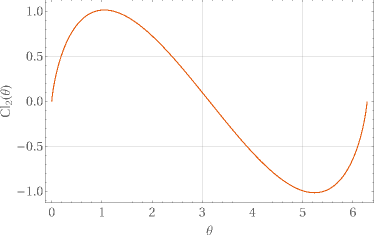
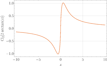
Figure 4: The left panel shows a plot of the Clausen function on the interval $[0,2\pi]$. The right panel displays the combination $\mathrm{Cl}_{2}(2\arctan x)$ as it appears in the results from section VIII.

The Clausen function is antisymmetric, periodic with period $2\pi$, and obeys $\mathrm{Cl}_{2}(\pi+\theta)=-\mathrm{Cl}_{2}(\pi-\theta)$. Furthermore it satisfies the duplication formula

$$\mathrm{Cl}_{2}(2\theta)=2\,\mathrm{Cl}_{2}(\theta)-2\,\mathrm{Cl}_{2}(\pi-\theta)\,.$$ (137)

Special values include $\mathrm{Cl}_{2}(0)=\mathrm{Cl}_{2}(\pi)=0$ and $\mathrm{Cl}_{2}(\pi/2)=\mathrm{C}$, where $\mathrm{C}=\sum_{n=0}^{\infty}\frac{(-1)^{n}}{(2n+1)^{2}}\approx 0.915965594$ denotes Catalan’s constant. The Clausen function attains its maximum at $\pi/3$ at the value $\mathrm{Cl}_{2}(\pi/3)=\mathrm{G}\approx 1.014941606$ called Gieseking’s constant.

Using the product expansion $\frac{\sin\pi z}{\pi z}=\prod_{n=1}^{\infty}\left(1-\frac{z^{2}}{n^{2}}\right)$ on the integrand of eq. (136), one obtains the series representation

$$\mathrm{Cl}_{2}(\theta)=\theta-\theta\log|\theta|-\sum_{n=1}^{\infty}\frac{(-1)^{n}B_{2n}}{2n\,(2n+1)}\frac{\theta^{2n+1}}{(2n)!}\,,$$ (138)

valid for $|\theta|<2\pi$, where $B_{2n}$ are the Bernoulli numbers. By keeping one logarithm explicit in the expansion, an even more rapidly convergent series is obtained,

$$\mathrm{Cl}_{2}(\theta)=3\theta-\theta\log\!\left|\,\theta\left(1-\frac{\theta}{2\pi}\right)\left(1+\frac{\theta}{2\pi}\right)\right|-2\pi\log\!\left(\frac{2\pi+\theta}{2\pi-\theta}\right)+\theta\sum_{n=1}^{\infty}\frac{\zeta_{2n}-1}{n(2n+1)}\left(\frac{\theta}{2\pi}\right)^{2n}\,,$$ (139)

which utilizes the quick convergence of the even zeta values $\zeta_{2n}\equiv\sum_{k=1}^{\infty}\frac{1}{k^{2n}}=(-1)^{n-1}\frac{(2\pi)^{2n}B_{2n}}{2(2n)!}$ to $1$ for large $n$. It was this series, truncated at $n=14$, Clausen used in his original calculation [54]. Other efficient numerical implementations can be found in [55, 56, 57].

The Clausen functions appearing in this paper all have arguments of the form $2\arctan x$ or $2\arctan x+2\arctan y$ – note that the second type can be brought into the form of the first by using the addition theorem of the arcus tangent (131). For real $x$, $y$ , we can express these Clausen functions in terms of the single-valued Bloch-Wigner dilogarithm $\mathrm{D}_{2}(z)=\mathrm{Im}\,\mathrm{Li}_{2}(z)+\arg(1-z)\log|z|$ by

$$\mathrm{Cl}_{2}(2\arctan x)=\mathrm{D}_{2}\!\left(\frac{\mathrm{i}-x}{\mathrm{i}+x}\right)\,\quad\text{respectively}\quad\mathrm{Cl}_{2}(2\arctan x+2\arctan y)=\mathrm{D}_{2}\!\left(\frac{\mathrm{i}-x}{\mathrm{i}+x}\,\frac{\mathrm{i}-y}{\mathrm{i}+y}\right).$$ (140)

The Bloch-Wigner dilogarithm is connected to the volume of ideal hyperbolic tetrahedra [58]. Concretely, in the upper-half space model, where the hyperbolic space $\mathfrak{H}_{3}$ is represented by $\mathbb{C}\times\mathbb{R}_{+}$, a tetrahedron with vertices $z_{0,1,2,3}\in\mathbb{C}$ has the hyperbolic volume

$$\mathbb{V}_{\mathfrak{H}}(z_{0},z_{1},z_{2},z_{3})=\mathrm{D}_{2}\!\left(\frac{z_{0}-z_{2}}{z_{0}-z_{3}}\,\frac{z_{1}-z_{3}}{z_{1}-z_{2}}\right).$$ (141)

The arguments of the Bloch-Wigner dilogarithms in eq. (140) are naturally represented as such cross ratios. In particular

$$\mathrm{Cl}_{2}(2\arctan x+2\arctan y)=\mathbb{V}_{\mathfrak{H}}(\mathrm{i},-\mathrm{i},x,-y)\,.$$ (142)

Another special function that is connected to the Clausen function is the inverse tangent integral $\mathrm{Ti}_{2}(x)=\int_{0}^{x}\frac{\mathrm{d}t}{t}\,\arctan t$, which can be expressed as

$$\mathrm{Ti}_{2}(x)=\arctan x\,\log x+\frac{1}{2}\mathrm{Cl}_{2}(2\arctan x)+\frac{1}{2}\mathrm{Cl}_{2}(\pi-2\arctan x)\,.$$ (143)

An analytic continuation of the Clausen function concatenated with an inverse tangent to complex arguments is given by

$$\mathrm{Cl}_{2}(2\arctan(z))=\frac{1}{2\mathrm{i}}\left[\mathrm{Li}_{2}\!\left(\frac{\mathrm{i}-z}{\mathrm{i}+z}\right)-\mathrm{Li}_{2}\!\left(\frac{\mathrm{i}+z}{\mathrm{i}-z}\right)\right]=\mathrm{i}\left(\mathrm{Li}_{2}\!\left(\frac{\mathrm{i}+z}{\mathrm{i}-z}\right)+\frac{1}{4}\log^{2}\!\left(\frac{z+\mathrm{i}}{z-\mathrm{i}}\right)+\frac{\pi^{2}}{12}\right).$$ (144)

It has a branch cut along the imaginary axis from $-\mathrm{i}$ to $\mathrm{i}$. In the high energy physics literature the Clausen function and its related constants appear in a variety of Feynman integral calculations, for example in [59, 60, 61, 62, 63, 64, 65, 66, 67, 68, 69, 70, 22].

References

- Schellekens [1981] A. Schellekens, Perturbative QCD and lepton pair production, Ph.D. thesis, Nijmegen University (1981).
- van Neerven [1986] W. van Neerven, Dimensional Regularization of Mass and Infrared Singularities in Two Loop On-shell Vertex Functions, Nucl. Phys. B 268, 453 (1986).
- Beenakker et al. [1989] W. Beenakker, H. Kuijf, W. van Neerven, and J. Smith, QCD Corrections to Heavy Quark Production in p anti-p Collisions, Phys. Rev. D 40, 54 (1989).
- Somogyi [2011] G. Somogyi, Angular integrals in d dimensions, J. Math. Phys. 52, 083501 (2011), arXiv:1101.3557 [hep-ph] .
- V. E. Lyubovitskij, F. Wunder and A. S. Zhevlakov [2021] V. E. Lyubovitskij, F. Wunder and A. S. Zhevlakov, New ideas for handling of loop and angular integrals in D-dimensions in QCD, JHEP 06 (2021), 066, arXiv:2102.08943 [hep-ph] .
- Wunder [2024] F. Wunder, Asymptotic behavior of angular integrals in the massless limit, Phys. Rev. D 109, 076022 (2024).
- Smirnov and Wunder [2024] V. A. Smirnov and F. Wunder, Expansion by regions meets angular integrals, JHEP 08, 138, arXiv:2405.13120 [hep-ph] .
- Bolzoni et al. [2011] P. Bolzoni, G. Somogyi, and Z. Trocsanyi, A subtraction scheme for computing QCD jet cross sections at NNLO: integrating the iterated singly-unresolved subtraction terms, JHEP 01 (2011), 059, arXiv:1011.1909 [hep-ph] .
- Anastasiou et al. [2013] C. Anastasiou, C. Duhr, F. Dulat, and B. Mistlberger, Soft triple-real radiation for Higgs production at N3LO, JHEP 07 (2013), 003, arXiv:1302.4379 [hep-ph] .
- Lillard et al. [2016] B. Lillard, T. M. P. Tait, and P. Tanedo, Kaluza-Klein gluons at 100 TeV: NLO corrections, Phys. Rev. D 94, 054012 (2016), arXiv:1602.08622 [hep-ph] .
- Kotlarski [2017] W. Kotlarski, Sgluons in the same-sign lepton searches, JHEP 02 (2017), 027, arXiv:1608.00915 [hep-ph] .
- Lionetti [2018] S. Lionetti, Subtraction of Infrared Singularities at Higher Orders in QCD, Ph.D. thesis, ETH Zürich (2018).
- Specchia [2018] C. Specchia, Perturbative Corrections to Inclusive and Differential Cross Sections for Higgs Production at the LHC, Ph.D. thesis, ETH Zürich (2018).
- Bahjat-Abbas et al. [2018] N. Bahjat-Abbas, J. Sinninghe Damsté, L. Vernazza, and C. White, On next-to-leading power threshold corrections in Drell-Yan production at N3LO, JHEP 10 (2018), 144, arXiv:1807.09246 [hep-ph] .
- Baranowski [2020] D. Baranowski, NNLO zero-jettiness beam and soft functions to higher orders in the dimensional-regularization parameter , Eur. Phys. J. C 80, 523 (2020), arXiv:2004.03285 [hep-ph] .
- Blümlein et al. [2020] J. Blümlein, A. De Freitas, C. Raab, and K. Schönwald, The initial state QED corrections to , Nucl. Phys. B 956, 115055 (2020), arXiv:2003.14289 [hep-ph] .
- Isidori et al. [2020] G. Isidori, S. Nabeebaccus, and R. Zwicky, QED corrections in at the double-differential level, JHEP 2020 (12), arXiv:2009.00929 [hep-ph] .
- Alioli et al. [2022] S. Alioli, A. Broggio, and M. A. Lim, Zero-jettiness resummation for top-quark pair production at the LHC, JHEP 01 (2022), 066, arXiv:2111.03632 [hep-ph] .
- Assi and Höche [2024] B. Assi and S. Höche, New approach to QCD final-state evolution in processes with massive partons, Phys. Rev. D 109, 114008 (2024), arXiv:2307.00728 [hep-ph] .
- Catani and Dhani [2023] S. Catani and P. K. Dhani, Collinear functions for QCD resummations, JHEP 2023 (3), 1, arXiv:2208.05840 [hep-ph] .
- Pal and Seth [2024] S. Pal and S. Seth, On production at next-to-leading power accuracy, Phys. Rev. D 109, 114018 (2024), arXiv:2309.08343 [hep-ph] .
- Devoto et al. [2024] F. Devoto, K. Melnikov, R. Röntsch, C. Signorile-Signorile, and D. M. Tagliabue, A fresh look at the nested soft-collinear subtraction scheme: NNLO QCD corrections to N-gluon final states in annihilation, JHEP 02, 016, arXiv:2310.17598 [hep-ph] .
- Rowe and Zwicky [2024] M. Rowe and R. Zwicky, Structure-dependent QED in , JHEP 07 (2024), 249, arXiv:2404.07648 [hep-ph] .
- Matsuura et al. [1989] T. Matsuura, S. Van Der Marck, and W. Van Neerven, The calculation of the second order soft and virtual contributions to the Drell-Yan cross section, Nucl. Phys. B 319, 570 (1989).
- Matsuura et al. [1990] T. Matsuura, R. Hamberg, and W. L. van Neerven, The contribution of the gluon-gluon subprocess to the Drell-Yan K-factor, Nucl. Phys. B 345, 331 (1990).
- Hamberg et al. [1991] R. Hamberg, W. Van Neerven, and T. Matsuura, A complete calculation of the order correction to the Drell-Yan K-factor, Nucl. Phys. B 359, 343 (1991).
- Mirkes [1992] E. Mirkes, Angular decay distribution of leptons from W bosons at NLO in hadronic collisions, Nucl. Phys. B 387, 3 (1992).
- Duke and Owens [1982] D. W. Duke and J. F. Owens, Quantum-chromodynamic corrections to deep-inelastic compton scattering, Phys. Rev. D 26, 1600 (1982).
- Hekhorn [2019] F. Hekhorn, Next-to-Leading Order QCD Corrections to Heavy-Flavour Production in Neutral Current DIS, Ph.D. thesis, University of Tübingen (2019), arXiv:1910.01536 [hep-ph] .
- Anderle et al. [2017] D. Anderle, D. de Florian, and Y. Rotstein Habarnau, Towards semi-inclusive deep inelastic scattering at next-to-next-to-leading order, Phys. Rev. D 95, 034027 (2017), arXiv:1612.01293 [hep-ph] .
- Wang et al. [2019] B. Wang, J. Gonzalez-Hernandez, T. Rogers, and N. Sato, Large Transverse Momentum in Semi-Inclusive Deeply Inelastic Scattering Beyond Lowest Order, Phys. Rev. D 99, 094029 (2019), arXiv:1903.01529 [hep-ph] .
- Gordon and Vogelsang [1993] L. Gordon and W. Vogelsang, Polarized and unpolarized prompt photon production beyond the leading order, Phys. Rev. D 48, 3136 (1993).
- Rein et al. [2024] D. Rein, M. Schlegel, and W. Vogelsang, Probing the polarized photon content of the proton in collisions at the EIC, Phys. Rev. D 110, 014041 (2024), arXiv:2405.04232 [hep-ph] .
- Ellis et al. [1980] R. K. Ellis, M. A. Furman, H. E. Haber, and I. Hinchliffe, Large Corrections to High p(T) Hadron-Hadron Scattering in QCD, Nucl. Phys. B 173, 397 (1980).
- Schlegel [2013] M. Schlegel, Partonic description of the transverse target single-spin asymmetry in inclusive deep-inelastic scattering, Phys. Rev. D 87, 034006 (2013), arXiv:1211.3579 [hep-ph] .
- Ringer and Vogelsang [2015] F. Ringer and W. Vogelsang, Single-Spin Asymmetries in W Boson Production at Next-to-Leading Order, Phys. Rev. D 91, 094033 (2015), arXiv:1503.07052 [hep-ph] .
- ’t Hooft and Veltman [1972] G. ’t Hooft and M. Veltman, Regularization and renormalization of gauge fields, Nucl. Phys. B 44, 189 (1972).
- C. G. Bollini and J. J. Giambiagi [1972] C. G. Bollini and J. J. Giambiagi, Dimensional Renormalization: The Number of Dimensions as a Regularizing Parameter, Nuovo Cim. B 12, 20 (1972).
- Salvatori [2024] G. Salvatori, The Tropical Geometry of Subtraction Schemes, (2024), arXiv:2406.14606 [hep-th] .
- Kotikov [1991] A. V. Kotikov, Differential equations method: New technique for massive Feynman diagrams calculation, Phys. Lett. B 254, 158 (1991).
- Remiddi [1997] E. Remiddi, Differential equations for Feynman graph amplitudes, Nuovo Cim. A 110, 1435 (1997), arXiv:hep-th/9711188 .
- Gehrmann and Remiddi [2000] T. Gehrmann and E. Remiddi, Differential equations for two-loop four-point functions, Nucl. Phys. B 580, 485 (2000), arXiv:hep-ph/9912329 .
- Henn [2013] J. M. Henn, Multiloop integrals in dimensional regularization made simple, Phys. Rev. Lett. 110, 251601 (2013), arXiv:1304.1806 [hep-th] .
- Henn [2015] J. M. Henn, Lectures on differential equations for Feynman integrals, J. Phys. A 48, 153001 (2015), arXiv:1412.2296 [hep-ph] .
- Badger et al. [2024] S. Badger, J. Henn, J. C. Plefka, and S. Zoia, Scattering Amplitudes in Quantum Field Theory, Lect. Notes Phys. 1021, pp. (2024), arXiv:2306.05976 [hep-th] .
- Binosi and Theußl [2004] D. Binosi and L. Theußl, JaxoDraw: A Graphical user interface for drawing Feynman diagrams, Comput. Phys. Commun. 161, 76 (2004), arXiv:hep-ph/0309015 .
- Laporta [2000] S. Laporta, High-precision calculation of multiloop Feynman integrals by difference equations, Int. J. Mod. Phys. A 15, 5087 (2000), arXiv:hep-ph/0102033 .
- ’t Hooft and Veltman [1979] G. ’t Hooft and M. J. G. Veltman, Scalar One Loop Integrals, Nucl. Phys. B 153, 365 (1979).
- Besier et al. [2019] M. Besier, D. Van Straten, and S. Weinzierl, Rationalizing roots: an algorithmic approach, Commun. Num. Theor. Phys. 13, 253 (2019), arXiv:1809.10983 [hep-th] .
- Euler [1781] L. Euler, De mensura angulorum solidorum, Acta Academiae Scientiarum Imperialis Petropolitanae , 31 (1781).
- Eriksson [1990] F. Eriksson, On the measure of solid angles, Mathematics Magazine 63, 184 (1990).
- Ahmed et al. [2024] T. Ahmed, S. M. Hasan, and A. Rapakoulias, Phase-space integrals through Mellin-Barnes representation, (2024), arXiv:2410.18886 [hep-ph] .
- L. Lewin [1981] L. Lewin, Polylogarithms and Associated Functions (Elsevier, 1981).
- Clausen [1832] T. Clausen, Über die Funktion etc., Journal für die reine und angewandte Mathematik 8, 298 (1832).
- Wood [1968] V. E. Wood, Efficient calculation of Clausen’s integral, Math. Comp. 22, 883 (1968).
- Kolbig [1995] K. S. Kolbig, Chebyshev coefficients for the Clausen function , J. Comput. Appl. Math. 64, 295 (1995).
- Wu et al. [2010] J. Wu, X. Zhang, and D. Liu, An efficient calculation of the Clausen functions , BIT Numerical Mathematics 50, 193 (2010).
- Zagier [2007] D. Zagier, The dilogarithm function, in Frontiers in Number Theory, Physics, and Geometry II: On Conformal Field Theories, Discrete Groups and Renormalization (Springer, 2007) pp. 3–65.
- Lu and Perez [1992] H. J. Lu and C. A. Perez, Massless one loop scalar three point integral and associated Clausen, Glaisher and L functions, (1992).
- Wagner [1996] P. Wagner, A volume formula for asymptotic hyperbolic tetrahedra with an application to quantum field theory, Indagationes Mathematicae 7, 527 (1996).
- Davydychev and Delbourgo [1998] A. I. Davydychev and R. Delbourgo, A Geometrical angle on Feynman integrals, J. Math. Phys. 39, 4299 (1998), arXiv:hep-th/9709216 .
- Broadhurst [1998] D. J. Broadhurst, Solving differential equations for three loop diagrams: Relation to hyperbolic geometry and knot theory, (1998), arXiv:hep-th/9806174 .
- Broadhurst [1999] D. J. Broadhurst, Massive three - loop Feynman diagrams reducible to SC* primitives of algebras of the sixth root of unity, Eur. Phys. J. C 8, 311 (1999), arXiv:hep-th/9803091 .
- Davydychev and Kalmykov [2001] A. I. Davydychev and M. Y. Kalmykov, New results for the epsilon expansion of certain one, two and three loop Feynman diagrams, Nucl. Phys. B 605, 266 (2001), arXiv:hep-th/0012189 .
- Davydychev and Kalmykov [2004] A. I. Davydychev and M. Y. Kalmykov, Massive Feynman diagrams and inverse binomial sums, Nucl. Phys. B 699, 3 (2004), arXiv:hep-th/0303162 .
- Czakon [2005] M. Czakon, The Four-loop QCD beta-function and anomalous dimensions, Nucl. Phys. B 710, 485 (2005), arXiv:hep-ph/0411261 .
- Binger and Brodsky [2006] M. Binger and S. J. Brodsky, The Form-factors of the gauge-invariant three-gluon vertex, Phys. Rev. D 74, 054016 (2006), arXiv:hep-ph/0602199 .
- Adams et al. [2015] L. Adams, C. Bogner, and S. Weinzierl, The two-loop sunrise integral around four space-time dimensions and generalisations of the Clausen and Glaisher functions towards the elliptic case, J. Math. Phys. 56, 072303 (2015), arXiv:1504.03255 [hep-ph] .
- Chicherin and Sotnikov [2020] D. Chicherin and V. Sotnikov, Pentagon Functions for Scattering of Five Massless Particles, JHEP 20 (2020), 167, arXiv:2009.07803 [hep-ph] .
- Abreu et al. [2022] S. Abreu, M. Becchetti, C. Duhr, and M. A. Ozcelik, Two-loop master integrals for pseudo-scalar quarkonium and leptonium production and decay, JHEP 09, 194, arXiv:2206.03848 [hep-ph] .