Anyon Superconductivity from Topological Criticality in a Hofstadter-Hubbard Model

Abstract

The identification of novel mechanisms for superconductivity is a longstanding goal in theoretical physics. In this work, we argue that the combination of repulsive interactions and high magnetic fields can generate electron pairing, phase coherence and superconductivity. Inspired by the large lattice constants of moiré materials, which make large flux per unit cell accessible at laboratory fields, we study the triangular lattice Hofstadter-Hubbard model at one-quarter flux quantum per plaquette, where previous literature has argued that a chiral spin liquid separates a weak-coupling integer quantum Hall phase and a strong-coupling topologically-trivial Mott insulator. We argue that topological superconductivity emerges upon doping in the vicinity of the integer quantum Hall to chiral spin liquid transition. We employ exact diagonalization and density matrix renormalization group methods to examine this theoretical scenario and find that electronic pairing indeed occurs above the half-filled ground states not just near the putative critical point but over a remarkably broad range of coupling strengths on both sides of criticality. On the chiral spin liquid side, our results provide a concrete model realization of the storied mechanism of anyon superconductivity. Our study thus establishes a beyond-BCS mechanism for electron pairing in a well-controlled limit, relying crucially on the interplay between electron correlations and band topology.

I Introduction

The search for electron pairing mechanisms that go beyond the well-established BCS/“pairing glue” paradigm exemplified by the electron-phonon mechanism has a long history [1, 2, 3]. A popular theoretical route has been to consider situations where charge is associated with topological excitations [4, 5, 6, 7, 8, 9, 10, 11, 12, 13]. The best known of these proposals are the resonating valence bond (RVB) [14, 15, 16, 17] and anyon superconductivity scenarios [18, 19, 20, 21, 22, 23, 24, 25, 26], where doping a quantum spin liquid with fractionalized charge excitations leads to superconductivity. In the anyon superconductivity approach, the starting point is the chiral spin liquid (CSL) phase introduced by Kalmeyer and Laughlin [27]. Although interest in the anyon mechanism for superconductivity in the context of high-$T_{c}$ cuprates has waned, it remains a remarkable theoretical example of superconductivity emerging from a chiral insulator.

Spin liquid phases have proven elusive, and even where they are proposed to appear, the lowest-energy charge excitations are often electronic rather than topological. The triangular lattice Hubbard model has been reported to host a chiral spin liquid (CSL) at intermediate coupling [28, 29, 30, 31], which competes closely with metallic and ordered phases [32]. However, the existence of superconductivity at small hole doping in the relevant intermediate-coupling regime [33, 34] has not been clearly established. Indeed, a density matrix renormalization group (DMRG) analysis reports a metallic phase rather than a superconductor [35]. Furthermore, there is no proximal spin liquid in the weak-coupling regime where superconductivity has also been proposed [36, 37].

In this work, we show that superconductivity emerges naturally in the vicinity of topological criticality arising from a continuous transition between two topologically-distinct insulators. The crucial point is that a change in topology requires closing and reopening a gap at the transition, in this case a charge gap associated with a bosonic charge-$2e$ mode. Near the topological critical point, these bosonic modes are the lowest-energy local charge excitations, while unpaired electronic states appear only at higher energies, so that modest doping introduces naturally-paired superconducting carriers.

Importantly, this mechanism does not require strict quantum criticality. Superconductivity emerges in a finite window around the topological critical point and will therefore persist even if the transition is weakly-first-order or one of the phases is proximal but avoided. Its precursor, electron pairing, appears even on the finite system sizes accessible in our numerics. Our approach suggests that superconductivity can emerge in a regime incorporating both strong repulsive interactions and broken time reversal symmetry, a combination normally considered antithetical to pairing.

We illustrate the potential of this idea through explicit calculations in a microscopic Hofstadter-Hubbard model argued to host two symmetric insulating phases [38, 39]: an integer quantum Hall (IQH) phase at weak coupling, with unit Chern number for each spin species, and a CSL phase emerging upon increasing electron correlations via repulsive Hubbard interactions. The study of this model is motivated by its potential realization in transition metal dichalcogenide (TMD) moiré materials [38, 40], whose advent has transformed the landscape of realizing exotic quantum phases and enabled the controlled variation of their doping [41, 42, 43].

We present a parton treatment and an effective field theory approach that reveal low-energy Cooper pairs in the vicinity of the putative IQH-CSL critical point, and contend that doping in its vicinity leads to a superconductor. These expectations are then examined numerically with exact diagonalization (ED) and DMRG, which reveal that charge-$2e$ excitations are indeed the cheapest local charge excitations, per unit charge, over a remarkably broad range of parameters, a compelling precursor to superconductivity upon doping. On the CSL side, the state we obtain through our parton analysis in the vicinity of criticality has the properties previously derived for anyon superconductivity. However, the pairing extends beyond the CSL, well into the IQH side of the phase diagram where anyons cannot be invoked, consistent with the softening of the $2e$ gap by topological criticality. In Fig. 1(a), we present a schematic phase diagram in the plane of chemical potential $\mu$ and Hubbard $U$.

The remainder of the manuscript is organized as follows. In Sec. II, we introduce the Hofstadter-Hubbard model as well as its continuous and magnetic space group symmetries. In Sec. III, we provide a parton description of the putative topological critical point and the mechanism for obtaining superconductivity upon doping each side of the transition. In Sec. IV, we provide numerical evidence for electron pairing using both ED and DMRG. Sec. V is a summary and conclusion suggesting avenues for future research. Appendices present details of calculations mentioned in the main text.

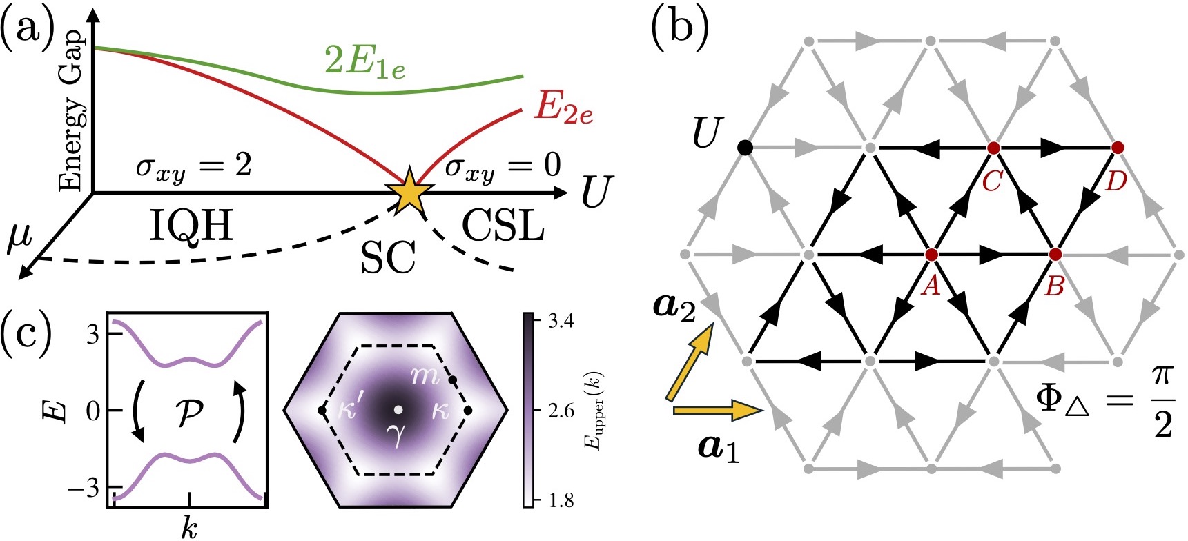
Figure 1: (a) Schematic depiction of the predicted energy gap to $2e$ excitations (red) and twice the energy of $1e$ excitations (green) at half filling of the Hofstadter-Hubbard model with $\Phi_{\triangle}=\pi/2$ flux per triangle as a function of interaction strength $U$ in the 2D limit. Proposed phase diagram in the plane of $U$ and chemical potential $\mu$. The star indicates a topological quantum phase transition from an integer quantum Hall (IQH) insulator to chiral spin liquid (CSL) at half filling. The dashed lines show the chemical potential required to add carriers and produce a chiral superconductor (SC) with topologically-protected edge modes. (b) Finite region of the two-dimensional model with $\Phi_{\triangle}=\pi/2$ flux per triangle, repulsive on-site interactions $U$, and Bravais vectors $\bm{a}_{1,2}$ indicated. The hoppings may be chosen to be $C_{6}$-invariant and imaginary (each arrow indicates an amplitude $-it$), with a four-site unit cell (sublattices $A$-$D$ in red). (c) Left: band structure at $\Phi_{\triangle}=\pi/2$ consisting of two bands related by particle-hole symmetry $\mathcal{P}$. Right: two-dimensional color map of energy as a function of momentum for the upper energy band over the Brillouin zone of the $2\times 2$ unit cell (note the bands are two-fold degenerate at every momentum).

II Model and Symmetries

The Hofstadter-Hubbard model (see Fig. 1b), with hoppings $t_{ij}$ from site $j$ to $i$ and on-site interaction $H_{I}$, is given by $H_{\text{HH}}=-\sum_{ij}t_{ij}c^{\dagger}_{i}c_{j}+H_{I}$. The hopping amplitudes are complex numbers with phases encoding the orbital magnetic flux [44]. In this work, we specialize to the triangular lattice with $\Phi_{\triangle}=\pi/2$ flux per triangle [38, 39] for which the hopping amplitudes can be chosen to be purely imaginary, so that the single-particle term in the Hamiltonian may be written as:

$$H_{0}=i\sum_{\langle ij\rangle}\tau_{ij}\left(c^{\dagger}_{i\sigma}c_{j\sigma}-c^{\dagger}_{j\sigma}c_{i\sigma}\right).$$ (1)

The arrows on bonds in Fig. 1(b) indicate our sign convention that the hopping from site $j$ to $i$ along an arrow has $\tau_{ij}=-t<0$, while hopping opposite an arrow has the opposite amplitude. We report energies in units of $t$.

The symmetries of $H_{0}$ are most clearly exposed by mapping to Majorana fermions, $c_{j\uparrow}=\frac{1}{2}(\chi_{1}^{j}+i\chi_{2}^{j})$ and $c_{j\downarrow}=\frac{1}{2}(\chi_{3}^{j}+i\chi_{4}^{j})$, where $\{\chi_{a}^{i},\,\chi_{b}^{j}\}=2\delta_{ab}\delta_{ij}$ so that $H_{0}$ takes the form [45, 46]:

$$H_{0}=\frac{i}{2}\sum_{1\leq a\leq 4}\sum_{\langle ij\rangle}\tau_{ij}\chi^{i}_{a}\chi^{j}_{a},$$ (2)

which is seen to have an O(4) symmetry, corresponding to proper/improper rotations of the Majorana four-component vector. The Hubbard interaction

$$H_{I}=U\sum_{i}(n_{i,\uparrow}-1/2)(n_{i,\downarrow}-1/2)$$ (3)

can be written in the Majorana representation as $H_{I}=-(U/4)\sum_{i}\chi^{i}_{1}\chi^{i}_{2}\chi^{i}_{3}\chi^{i}_{4}$. Note that the interaction breaks the O(4) symmetry of the hopping model down to SO(4). The operators in the determinant $-1$ sector, corresponding to improper rotations, are related to particle-hole transformations that flip the sign of $U$ (e.g., conjugating only the spin-up electrons) and are therefore not symmetries of the interacting theory. The particle-hole which preserves the sign of $U$ is a symmetry, identified in [39].

Contained in SO(4) are the spin $\mathrm{SU(2)}_{s}$ and pseudospin $\mathrm{SU(2)}_{c}$ symmetry subgroups [47, 48, 49, 45], though the latter reduces to the usual charge $\mathrm{U(1)}_{c}$ for generic long-range interactions. While the pseudospin symmetry has typically been regarded as a feature of only bipartite lattice Hubbard models [50], we highlight that it is more generally present whenever there exists a gauge in which the hoppings are purely imaginary. The pseudospin $\mathrm{SU}(2)_{c}$ symmetry will play an important role in our study of the topological phase transition in Sec. III.1.

The model is additionally symmetric under operators in the magnetic space group generated by the rotation $C_{6}$ and translation $T_{1}$ along the nearest-neighbor direction $\bm{a}_{1}$ (see Fig. 1b). Their explicit form, which we provide in App. SII, depends on the choice of gauge for the electron operators [51, 52]. However, they satisfy certain gauge-invariant generating relations which will prove important for interpreting the pairing symmetry in Sec. IV.3. Because the magnetic space group is a $U(1)_{c}$ extension [53], the overall $U(1)_{c}$ phase of each spatial symmetry is ambiguous. We make the following convenient choices: we fix $(C_{6})^{6}=1$, choose $T_{1}$ to satisfy $C_{2}T_{1}C_{2}^{\dagger}=T_{1}^{\dagger}$ which constrains it modulo a sign, and define rotated nearest-neighbor translations by $T_{j+1}=C_{6}^{j}T_{1}C_{6}^{-j}$. Moreover, due to the $\pi/2$ flux per triangle, one may verify the following gauge-invariant relations:

$$T_{2}T_{1} =(-1)^{N_{F}}T_{1}T_{2},\quad T_{5}T_{3}T_{1}=(\pm i)^{N_{F}},$$ (4)

where $N_{F}$ is the fermion number. The sign ambiguity in the second relation arises because our conventions do not fix the sign of $T_{1}$; we remedy this by choosing $+i$. When acting on charge-$2e$ pairs, with $N_{F}=2$, the first relation is trivial, but the second is not. This is the origin of the unorthodox pairing symmetry we uncover in Sec. IV.3.

III Parton Theory

III.1 Topological Criticality at Half-Filling

We introduce a parton construction that captures the effects of on-site $U$, in effect performing a Gutzwiller projection on the IQH wavefunction to obtain the CSL [54, 55]. This formalism reproduces the phase diagram of the half-filled model obtained in previous numerics [38, 39] and allows us to study the effects of doping. While it is possible to proceed by retaining the $\mathrm{SU(2)_{c}}$ pseudospin symmetry [50], we relegate this treatment to App. F and, for ease of presentation and analysis, derive here a slave-rotor theory retaining only $\mathrm{U(1)}_{c}$ along with $\mathrm{SU(2)}_{s}$. We begin by introducing a U(1) rotor variable $e^{i\theta}$ and its conjugate integer-valued “angular momentum” $L$ at each site [56]. We write the electron operator as $c^{\dagger}_{i,\sigma}=f^{\dagger}_{i,\sigma}\,e^{i\theta_{i}}$ where $f$ is a fermionic “spinon” carrying the electronic spin. The redundancy introduced by the rotors is alleviated by imposing the following constraint at each site:

$$L_{i}=f^{\dagger}_{i,\uparrow}f_{i,\uparrow}+f^{\dagger}_{i,\downarrow}f_{i,\downarrow}-1.$$ (5)

Note that a singly-filled site is represented by $L_{i}=0$, while the doublon/hole sites correspond to $L_{i}=\pm 1$. The Hubbard model can then be rewritten as [56]:

$$H=-\sum_{\langle ij\rangle,\sigma}t_{ij}e^{i(\theta_{i}-\theta_{j})}f^{\dagger}_{i,\sigma}f_{j,\sigma}+{\rm h.c.}+\frac{U}{2}\sum_{i}L_{i}^{2}.$$ (6)

To make progress, we adopt a mean field approach, replacing operator bilinears by their mean field values:

$$H_{\mathrm{MF}} =H_{f}+H_{\theta}$$ (7)

$$H_{f} =-\sum_{\langle ij\rangle,\sigma}\tilde{t}_{ij}f^{\dagger}_{i,\sigma}f_{j,\sigma}+{\rm h.c.}$$

$$H_{\theta} =-\sum_{\langle ij\rangle,\sigma}{Q}_{ij}e^{i(\theta_{i}-\theta_{j})}+{\rm h.c.}+\frac{U}{2}\sum_{i}L_{i}^{2},$$

where $Q_{ij}=t_{ij}\langle f^{\dagger}_{i,\sigma}f_{j,\sigma}\rangle$ and $\tilde{t}_{ij}=t_{ij}\langle e^{i(\theta_{i}-\theta_{j})}\rangle$. This mean field theory can be analyzed using the fact that the rotor fields see zero effective flux, unlike the previously-studied scenario of electrons subject to zero external flux [57, 58]. Let us summarize the main results, leaving the detailed analysis of this mean field theory to App. B. First, note that the $f$ fermions see the same net flux as the electrons and enter a Chern insulator phase. Since the rotor bosons then see no net flux, the Hamiltonian $H_{\theta}$ displays a superfluid-Mott transition on increasing $U$, corresponding to the electronic IQH-CSL transition. A mean-field treatment of $H_{\theta}$ locates this critical point (see App. B) at $U^{*}/t\approx 9.6$, not far from the transition point $U^{*}/t\approx 12$ estimated by iDMRG [38, 39].

Next, using Eq. (7), we show that the universal response properties of the spinon-rotor mean field solutions are consistent with that of the IQH and CSL observed numerically in Refs. [38, 39]. As usual, we introduce a gauge field on bonds to account for gauge fluctuations about the mean field solution [59], giving ${Q}_{ij}\rightarrow Qe^{-ia_{ij}}$ and $\tilde{t}_{ij}\rightarrow\tilde{t}_{ij}e^{+ia_{ij}}$. Further, we introduce a gauge field $A$ ($A_{s}$) coupled minimally to the rotors (spinons) to probe the charge (spin) response. We note that the spinons $f$ remain gapped throughout the transition, implying a spin gap. Restricting to energies below this gap, we may integrate out the spinons; the unit Chern number for each spin species yields the following Chern-Simons terms [60]:

$${\mathcal{L}}_{\mathrm{csl}}=\frac{2}{4\pi}(a\wedge d\,a+A_{s}\wedge d\,A_{s}).$$ (8)

We employ the notation $a\wedge da=\epsilon_{\mu\nu\lambda}a_{\mu}\partial_{\nu}a_{\lambda}$, where summation over Greek spacetime indices is implicit and $\epsilon$ is the three-dimensional antisymmetric tensor. Having addressed the behavior of spinons, we now turn to the rotor charge excitations. Since we are interested here in long wavelength properties, it is convenient to pass to the continuum limit and utilize a coarse-grained “soft spin” description, replacing $\psi\sim e^{i\theta}$ and introducing a potential $V(\psi)=m^{2}|\psi|^{2}+\lambda|\psi|^{4}$. Note, there is only a single species of $\psi$ corresponding to a single minimum in the rotor dispersion, a consequence of the vanishing average flux that it experiences. Tuning the sign of $m^{2}$ from positive to negative induces condensation of $\psi$, as we describe below. The resulting effective field theory is:

$${\mathcal{L}}=|{\mathcal{D}}_{A-a}\psi|^{2}-V(\psi)+\frac{2}{4\pi}a\wedge d\,a+\frac{2}{4\pi}A_{s}\wedge d\,A_{s},$$ (9)

where ${\mathcal{D}}^{\mu}_{b}=\partial^{\mu}-ib^{\mu}$, and we have taken advantage of field rescaling to bring it into this form. Note that the time component $a_{0}$ is introduced to implement the on-site constraint Eq. (5). We now consider the two phases.

Phase I: $m^{2}<0,\,\langle\psi\rangle\neq 0$. Here, in the small-$U$ limit we expect the rotor variables to “condense,” which actually corresponds to a Higgs condensate that forces $\nabla\times(a-A)=0$. This leads to the following effective action: ${\mathcal{L}}_{\mathrm{I}}[a,A,A_{s}]=\frac{2}{4\pi}A\wedge dA+\frac{2}{4\pi}A_{s}\wedge dA_{s}$. Thus we have an insulator without intrinsic topological order, with precisely the charge and spin quantum Hall conductance of the spin-singlet integer quantum Hall state, namely $\sigma_{xy}=2\cdot e^{2}/h$ and $\sigma^{s}_{xy}=2\cdot\hbar/8\pi$. The latter describes the quantized response of spin to a Zeeman gradient, termed the spin quantum Hall effect [61] and distinct from the quantum spin Hall effect [62, 63].

Phase II: $m^{2}>0,\,\langle\psi\rangle=0$. Now, in the larger-$U$ regime, the rotor condensate disappears and the $\psi$ field is gapped. The low-energy effective action in this phase is then ${\mathcal{L}}_{\mathrm{II}}[a,A,A_{s}]=\frac{2}{4\pi}a\wedge da+\frac{2}{4\pi}A_{s}\wedge dA_{s}={\mathcal{L}}_{\mathrm{csl}}$. While the spin response is the same as in Phase I (guaranteed by the spin gap being maintained throughout), the charge response is now trivial. Semion topological order now arises from the dynamical $U(1)_{2}$ Chern-Simons term. These are the characteristic properties of the CSL.

Critical Point: The critical point corresponds to setting $m^{2}=0$ in Eq. (9), so that the $\psi$ fields are gapless. Some intuition for these fields can be gained by recognizing that the fractionalized spin-$1/2$ semion excitations in the CSL can combine with the electron to give a charge-$e$ spin-singlet excitation, which is nothing but the non-local $\psi$ field, which becomes gapless at the transition.

The fact that the quantized charge response changes between the IQH and CSL phases implies that if the IQH-CSL transition is continuous, the charge gap must close at the transition. Furthermore, since the spin gap is always open, electrons remain gapped, pointing to spin-singlet Cooper pairs being the cheapest local charge excitations. This will be numerically demonstrated in Sec. IV. The following viewpoint helps clarify why Cooper pairs play such a prominent role at the transition.

Consider the following mapping to an equivalent transition between a trivial Mott insulator and $\nu=-1/2$ Laughlin state of charge-$2e$ Cooper pairs [64, 65]. This can be seen by “stacking” an invertible $\nu=-2$ IQH phase above Phases I and II [58]. This trivializes both the spin and charge response of the IQH and identifies the CSL with a phase with Hall conductance $\sigma_{xy}=-\frac{1}{2}\frac{(2e)^{2}}{h}$ but no spin response, namely a Laughlin liquid of Cooper pairs. This transition can therefore be viewed as a plateau transition, which rationalizes there being gapless Cooper pairs at the critical point. In Ref. [65], this transition is expressed both in a form equivalent to Eq. (9) and as its fermionic dual, a $\mathrm{QED}_{3}$-Chern-Simons theory [64]. Moreover, on the basis of a conjectured “level-rank” duality [66], it is argued that the theory possesses an emergent SO(3) symmetry [67], which rotates the boson density into the boson creation and annihilation operators. This suggests that not only charge-$2e$ Cooper pairs, but also their conserved density, become gapless at the critical point and that these modes belong to a triplet of the emergent SO(3) symmetry. Since the conserved density in a (2 + 1)D conformal field theory has protected scaling dimension 2, the Cooper pair insertion operator is expected to have the same scaling dimension [65].

We contend that our lattice model provides a microscopic realization of this transition, with the pseudospin $\mathrm{SU(2)}_{c}$ symmetry (introduced in Sec. II) explicitly implementing the emergent SO(3) symmetry. Employing the non-abelian slave-rotor formalism [50], we exploit this symmetry to derive an SU(2) Chern-Simons theory invariant under the full pseudopin symmetry (see App. F for details), generalizing Eq. (9). The conserved current of this theory, which describes the bosonic modes that go gapless at criticality, manifestly transforms as an SO(3) vector under the pseudospin symmetry, thus confirming the predictions presented above [65].

III.2 Finite Doping

In this section, we turn to finite doping and to the phase diagram of Fig. 1(a). We describe how each of the insulating phases considered above naturally gives rise to superconductivity upon doping, with proximity to topological criticality playing the crucial role of relegating electronic excitations to high energies. On the IQH side, we argue this occurs via the condensation of low-lying charge-$2e$ modes, while on the CSL side we show how superconductivity arises within a parton description of the low-lying fractionalized charge carriers. We conclude by elucidating a remarkable connection to the mechanism of anyon superconductivity and the possible microscopic realization of higher-charge superconductivity.

Starting from the IQH (or Phase I), the persistence of the spin gap and softening of the $2e$ gap by topological criticality implies that doped charges enter as Cooper pair excitations, i.e., bound states of electrons. This can be seen from the effective theory (Eq. 9) in the phase where $\psi$ is condensed. Shifting variables $a\rightarrow a+A$ and introducing a chemical potential via $A_{0}\to A_{0}-\mu$, we identify a coupling between chemical potential and flux: $-2\frac{\mu}{2\pi}\nabla\times\bm{a}$ where $\nabla\times\bm{a}=\partial_{x}a_{y}-\partial_{y}a_{x}$, which implies that charges enter as vortices of the $\psi$ condensate. In particular, by flux quantization $\int\nabla\times\bm{a}\in 2\pi\mathbb{Z}$, they are forced to enter as charge-$2e$ objects, or Cooper pairs.

Per unit cell of the triangular lattice, these pairs experience $2\pi$ external flux, twice that of their constituent electrons. Thus, magnetic translations do not enforce degenerate minima in the energy landscape of boson excitations, unlike at generic flux fractions where the Cooper pair effective mass would also be suppressed by a narrower bosonic Hofstadter bandwidth . In fact, in Sec. IV we provide numerical evidence that there is a dispersive, non-degenerate $2e$ bound state. At fixed $U/t=6$ on the $4\times 4$ torus, in Sec. IV.1 we estimate its effective mass to be $m_{\rm Cooper}\approx 1.3\,m^{\star}$, where $m^{\star}=\hbar^{2}/ta^{2}$, thus providing an order-of-magnitude estimate of the Cooper pair effective mass in the IQH phase. Moreover, we expect the low-lying Cooper pairs to have a characteristic size $\ell_{c}$ controlled by the spin gap. At sufficiently low density of dopants relative to both $\ell_{c}^{-2}$ and $\xi^{-2}$, where $\xi$ is the charge-$2e$ correlation length (see App. D), we therefore have a dilute gas of short-range interacting bosons, which are expected to enter a superfluid phase. Due to the unique boson dispersion minimum, we expect this condensate to respect all the crystalline symmetries.

The charge and spin response of the spin-singlet IQH insulator are $\sigma_{xy}=2\cdot e^{2}/h$ and $\sigma^{s}_{xy}=2\cdot\hbar/8\pi$, respectively, with edge chiral central charge $c_{-}=2$. On condensing spin-singlet Cooper pairs, the spin Hall response is unaffected since the spin sector remains gapped. However, including their Meissner response removes the quantization of charge Hall conductance, while the chiral central charge is unchanged [69]. Altogether, this predicts edge states usually associated with the so-called weak-pairing “$d+id$” superconductors [61]. However, as we will see in Sec. IV, we are far from the weak-pairing limit, so that the actual symmetry of the Cooper pair wavefunction is unrelated to the topological properties and edge states of the superconductor [70]. Moreover, as we later discuss in Sec. IV.3, the terminology regarding pairing symmetry must be adapted to the present scenario of magnetic space group symmetries.

Starting from the CSL (or Phase II) is more involved. Since we now have fractionalized elementary excitations, we appeal to the parton description. We consider doping a finite charge density of $0<y\ll 1$ holes per site, which requires that the rotor density be $\langle L_{i}\rangle=-y$. The constraint Eq. (5) correspondingly demands a depletion of spinons relative to integer filling: $\langle n^{f}_{i\uparrow}+n^{f}_{i\downarrow}\rangle=1-y$, which seemingly poses a problem since we expect the spin gap, and hence the spinon gap, to remain open upon light doping. Fortunately, since the spinons occupy bands with Chern number $C_{\uparrow}=C_{\downarrow}=1$, their density can be tuned by introducing additional gauge flux $n_{\phi}\equiv(\nabla\times\bm{a})/2\pi=-y/2$.

To evaluate the resulting physical behavior and elucidate the possibility of superconductivity, let us concentrate on hole doping and replace our rotor with a hardcore bosonic “holon” $b$ on each site, with $n_{b}=b^{\dagger}b\in\{0,1\}$, and write $c^{\dagger}_{\sigma}=bf^{\dagger}_{\sigma}$. The Hilbert space on each site is restricted to empty and single-electron states, which both satisfy the slave-boson constraint $n_{b}=1-n_{f}$ [57]. Following our previous analysis but with the canonical boson $b$ rather than the rotor, integrating out $f$ leaves:

$${\mathcal{L}}_{\rm doped} = b^{*}\left(i\partial_{t}+a_{0}-A_{0}\right)b-|\vec{D}_{a-A}b|^{2}-V(b)$$ (10)

$$+\frac{2}{4\pi}a\wedge da+\frac{2}{4\pi}A_{s}\wedge dA_{s}.$$

This theory incorporates the feature that the density of holons is constrained to be $n_{b}=-2n_{\phi}$, seen from the equation of motion for $a_{0}$. While there are a variety of possible phases of bosons at the filling $\nu_{\rm holon}=-2$, a very natural one is the bosonic integer quantum Hall (bIQH) state with even integer Hall conductivity [71], a symmetry protected topological phase (SPT) [72, 73] (where the protecting $U(1)$ symmetry is taken to be the gauge “symmetry”). The bIQH phase hosts symmetry-protected counter-propagating edge states and has no intrinsic topological order. Thus it is entirely captured by its effective response theory [71, 73], probed by the gauge field combination $a-A$, namely $\Delta{\mathcal{L}}_{\rm holon}(a,A)=-\frac{2}{4\pi}(a-A)\wedge d(a-A)$. Adding this to the effective theory for Phase II we obtain the finite-doping theory in which, importantly, the Chern-Simons term for $a$ cancels out, implying the absence of intrinsic topological order:

$${\mathcal{L}}_{\rm doped}=\frac{2}{2\pi}a\wedge dA-\frac{2}{4\pi}A\wedge dA+\frac{2}{4\pi}A_{s}\wedge dA_{s}.$$ (11)

That this describes a superconductor can be seen by integrating out $a$, leading to the Meissner response $dA=0$; the Chern-Simons charge response is then subdominant. An intuitive understanding is given by the Ioffe-Larkin rule for addition of spinon and holon resistivity tensors [74, 75, 76, 77], which describe opposite Hall responses:

$$\rho_{\rm spinon}=-\rho_{\rm holon}=\frac{1}{2}\begin{pmatrix}0&1\\ -1&0\end{pmatrix}.$$ (12)

The combined resistivity tensor $\rho=\rho_{\rm spinon}+\rho_{\rm holon}$ thus vanishes, characteristic of superconductivity [57]. Further, we can see from the first term in Eq. (11) that a fundamental flux $\int\nabla\times\bm{a}=2\pi$ couples minimally to the external gauge field $A$ and binds $2e$ charge, i.e., is the Cooper pair. Hence this is a superconductor of Cooper pairs, and the monopole operator that inserts a unit of flux is their creation operator. On the other hand, we see that the quantized spin response remains unchanged since the spin gap is maintained on doping. Hence, the superconductor obtained upon doping the CSL has precisely the same topological properties as that originating from the IQH phase. This justifies the phase diagram shown in Fig. 1(a).

Relation to Anyon Superconductivity—The discussion above has a close correspondence with anyon (or more precisely semion) superconductivity, proposed in Refs. [18, 19, 20, 21, 22, 23, 24, 25, 26]. These works argued that a finite-density gas of charge-$e$ semions, obtained for instance by doping a CSL, can realize a superconducting state. This problem can be mapped to that of bosons $b^{\prime}$ attached to $\pi$ statistical flux, which transmutes their statistics to those of the original semions [78]. In this description, the boson and flux densities are therefore related by $n_{b^{\prime}}=-2n_{\phi}$, exactly the relation satisfied by the slave bosons in Eq. (10). The analysis following that equation provides a direct link between our long-wavelength theory of the doped CSL, derived for the Hubbard-Hofstadter model, and the effective theory of semion superconductivity, most transparently its bosonic formulation developed in Ref. [78]. Crucially, our analysis provides an alternative explanation of the semion superconductor by describing it as a bIQH phase of the $b^{\prime}$ bosons [57]. We emphasize that the advantage of our setup lies in the fact that proximity to topological criticality in the CSL phase ensures that doped semions (carrying charge-$e$ and no spin) are energetically more favorable than electrons.

The bIQH characterization also offers insight into the possible microscopic realization of charge-$Ne$ superconductivity with $N\in 2\mathbb{Z}$. Consider electrons in the fundamental representation of a flavor $\mathrm{SU}(N)$ symmetry and apply a background flux of $2\pi/N$ per unit cell. At a density of one electron per site, the non-interacting phase is an IQH insulator with $\sigma_{xy}=Ne^{2}/h$ where the lowest Hofstadter band is filled by all $N$ flavors. On increasing $U$, we expect to realize a CSL with $\mathrm{SU}(N)_{1}$ (or equivalently $\mathrm{U}(1)_{N}$) topological order and chiral central charge $c_{-}=N-1$ [55]. A possible critical theory is then the $\mathrm{SU}(N)$ analogue of Eq. (9) above:

$$\mathcal{L}=|{\mathcal{D}}_{A-a}\chi|^{2}-V(\chi)+\frac{N}{4\pi}a\wedge d\,a,$$ (13)

where the IQH and CSL again correspond to the condensed and gapped phases for $\chi$, respectively. Upon doping, superconductivity can arise if the excess bosons enter a bIQH phase, yielding a Hall contribution $\frac{M}{4\pi}a\wedge da$ where $M$ is necessarily even [71]. Therefore, the Chern-Simons term in Eq. (13) may be canceled out, and a conventional superconductor can arise, for even integer $N$. Furthermore, these correspond to a condensate of charge-$Ne$ electron composites which are singlets under the SU($N$) and clearly can only condense for even $N$. Note that the charge-$e$ anyons in this scenario have statistical angle $\theta=\pi/N$, distinct from $\pi(1-1/N)$ in the classic anyon superconductivity scenario [79]. They only agree for the special case of $N=2$, i.e., semion superconductivity, considered in this work.

Even at $N=2$, it maybe tempting to view anyon superconductivity as arising from the binding of pairs of charge-$e$ semions into bosons, that then condense. We remark however that this route would leave the remaining semionic excitations deconfined, resulting in a very different fractionalized superconductor “SC^∗” [80] that retains semionic excitations. Due to the absence of a Chern-Simons term for $a$ in Eq. (11), the anyon superconductor mechanism evidently yields a superconductor of the more conventional, unfractionalized variety [79, 78].

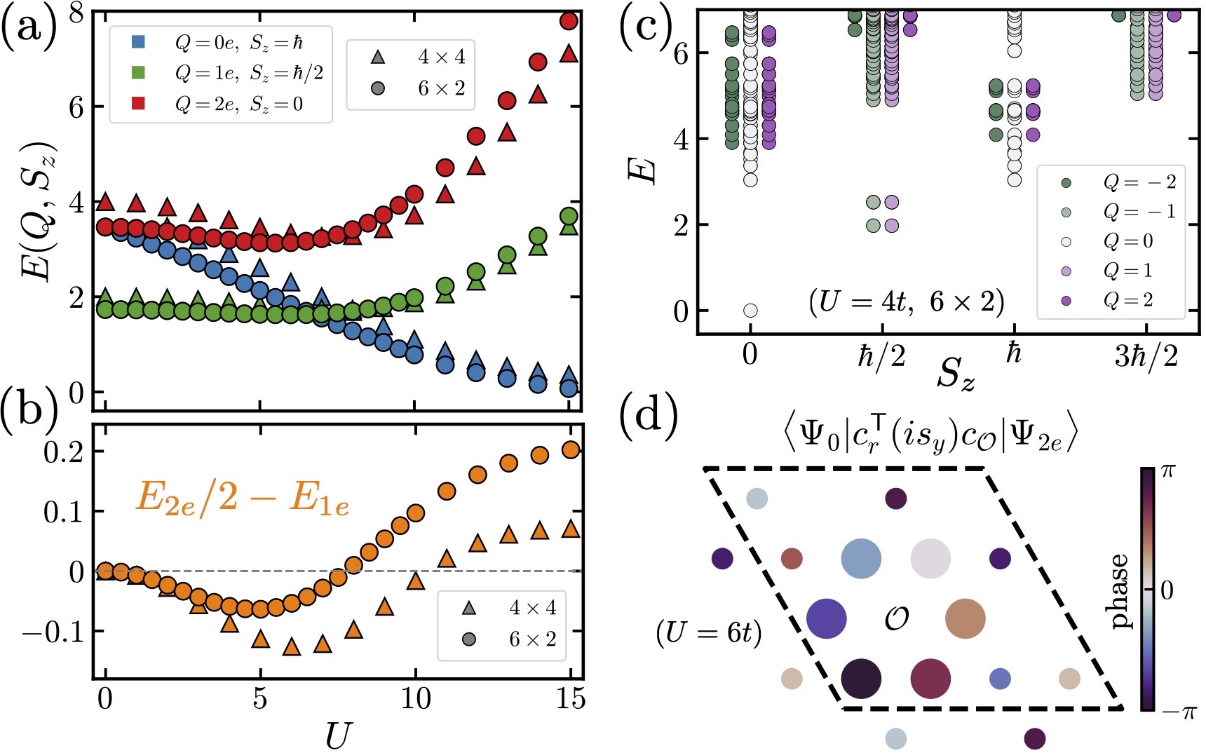
Figure 2: (a) Exact diagonalization (ED) energies of the lowest-lying states in three charge sectors (indicated in legend) for both the $4\times 4$-site (triangular markers) and $6\times 2$-site systems (circles). (b) Plot of $E_{2e}/2-E_{1e}$ vs. $U$, whose negative value indicates electron pairing. (c) ED energy spectrum on the $6\times 2$-site torus at $U/t=4$. The energies are arranged by total spin $S_{z}$ and electric charge $Q$ (indicated in legend), and organize into multiplets of the spin and pseudospin SU(2) symmetries. (d) Overlap of the spin-singlet pairing operator $c^{\mathsf{T}}_{\bm{r}}(is_{y})c_{\mathcal{O}}$ between the half-filled ground state and two-electron excitation for all sites $\bm{r}$ on a $4\times 4$-site torus at $U/t=6$, with origin indicated by $\mathcal{O}$. Its magnitude and phase are specified by marker area and color, respectively.

IV Numerical evidence for Cooper pairing

In the preceding section, we presented field-theoretic arguments for the nature of the putative critical theory and its excitations, as well as the intriguing possibility of topological superconductivity upon doping near this critical point. Here, we provide explicit numerical evidence for an important precursor to superconductivity, electron pairing above the half-filled ground states.

IV.1 Exact Diagonalization

We first investigate the system using exact diagonalization (ED). We focus on $6\times 2$ and $4\times 4$-site systems, the latter being the largest we can access. We diagonalize the Hamiltonian at the particle-hole-symmetric point $\mu=0$, and organize the spectrum by the charge $Q$ and spin $S_{z}$ quantum numbers, taking the convention where the half-filled ground state has $Q=S_{z}=0$ and zero energy. To construct the $6\times 2$ torus, we identify points separated by the vectors $6\bm{a}_{1}$ and by $2\bm{a}_{2}-4\bm{a}_{1}$. On the $4\times 4$ system, we identify points related by $4\bm{a}_{1}$ and $4\bm{a}_{2}$ (see Fig. 1(b) for the definition of the lattice vectors $\bm{a}_{1,2}$).

In Fig. 2(a), we plot the energies of the lowest-lying excited states in the charge sectors $(Q,S_{z})$ specified by $\{(0e,\hbar),(1e,\hbar/2),(2e,0)\}$, for both the $6\times 2$ and $4\times 4$ systems. While we focus on the electron-doped side, adding holes is energetically equivalent under particle-hole symmetry. The lowest $0e$ excitation energy decreases monotonically as a function of $U$. On the other hand, both $1e$ and $2e$ exhibit minima at intermediate coupling: for the $6\times 2$ system, these occur at $U^{\mathrm{min}}_{1e}/t\simeq 6.0$ and $U^{\mathrm{min}}_{2e}/t\simeq 5.5$, whereas on the $4\times 4$ torus these values increase to $U^{\mathrm{min}}_{1e}/t\simeq 8$ and $U^{\mathrm{min}}_{2e}/t\simeq 7$.

The ED calculation convincingly demonstrates that the lowest-lying charge excitations are paired over a remarkably broad range of interaction strengths $U$. Specifically, the energy $E_{2e}$ of the lowest-lying charge-$2e$ state is less than that of two individual electronic excitations, i.e., $E_{2e}-2E_{1e}<0$. We plot this quantity in Fig. 2(b), which we find to be negative in the range $0<U/t<7.5$ for the $6\times 2$ system and over an even broader range $0<U/t<10$ for the larger $4\times 4$ system. The maximum magnitude of the pairing energy increases from $0.06t$ to $0.13t$ between the two systems, constituting $4\%$ and $7\%$ of the corresponding $1e$ energies, respectively. The location of this maximum is $U_{\mathrm{max}}/t\simeq 5$ for the $6\times 2$ system, increasing to $U_{\mathrm{max}}/t\simeq 6$ on the larger $4\times 4$ torus. Though these features occur at smaller interaction strength than the expected IQH-CSL transition point $U/t\approx 12$ reported by previous cylinder iDMRG studies [38, 39], we anticipate the location will continue to shift to larger $U$ with increasing system size.

The numerical observation of pairing is important confirming evidence for topological criticality and the associated softening of charge-$2e$ modes. Moreover, as argued in Sec. III.2, the existence of pairing in the IQH phase is a direct precursor to strong-pairing superconductivity, and is likewise expected for the CSL near criticality. To estimate the Cooper pair effective mass, important for establishing phase stiffness, we thread small external flux $\varphi$ through the torus and compute the change in the charge-$2e$ energy $E_{2e}$. For concreteness, we fix $U/t=6$ on the $4\times 4$ torus, where pairing is maximal, though on larger systems we expect this point to reside deep in the IQH phase (see Refs. [38, 39]). At small $\varphi$, we obtain a quadratic fit $E_{2e}(\varphi)/t\approx 5.01(\varphi/2\pi)^{2}$. Threading $2\pi$ flux shifts the total two-electron momentum $\bm{q}$ by $2/L$ times a primitive reciprocal vector of magnitude $4\pi/a\sqrt{3}$, where $L=4$ is the length of the torus. Matching the dispersion to $\hbar^{2}q^{2}/2m_{\mathrm{Cooper}}$ with $\varphi/2\pi=qa\sqrt{3}/2\pi$, we estimate $m_{\mathrm{Cooper}}\approx 1.3\,\hbar^{2}/ta^{2}$ at the chosen system size and interaction strength, providing an order-of-magnitude estimate for the pair effective mass in the IQH phase.

We note that the pairing energy $E_{2e}-2E_{1e}$ cannot be positive in the thermodynamic limit because it is always possible to create a pair of well-separated $1e$ excitations with energy equal to that of independent electrons. Its taking positive values for $U/t>7.5$ and $U/t>10$ on the $6\times 2$ and $4\times 4$ systems, respectively, is therefore a finite size effect. Given that the interactions are repulsive, the observed (negative) electron pairing energy at smaller $U$ has no similarly-compelling finite-size explanation, thus pointing to topological criticality as its origin. Furthermore, the fact that pairing extends down to seemingly arbitrarily-small values (probed down to $U/t=10^{-3}$) suggests a weak-coupling origin complementary to pairing induced strictly by proximity to criticality, which we further elucidate in Sec. IV.4 by a small-$U$ perturbative calculation on much larger systems.

Each of the systems under consideration possesses the $\mathrm{SO(4)}$ symmetry explicated in Sec. II. Accordingly, we observe that the ED spectrum organizes into multiplets of the spin and pseudospin $\mathrm{SU(2)}$ symmetries. This is displayed in Fig. 2(c) for the $6\times 2$ torus at $U/t=4$, in which eigenstates with fixed spin $S_{z}$ but different total charge $Q$ are found to populate multiplets of the pseudospin $\mathrm{SU(2)}_{c}$. For both system sizes, the $(Q,S_{z})=(0e,\hbar)$ state in Fig. 2(a) belongs to a spin-triplet pseudospin-singlet irreducible representation, while the $(Q,S_{z})=(2e,0)$ branch is a spin-singlet pseudospin-triplet.

We remark that pairing was not observed on the smaller $4\times 2$ system, nor at $6\times 2$ with the identification $\bm{r}\sim\bm{r}+2\bm{a}_{2}\sim\bm{r}+6\bm{a}_{1}$, though we remind the reader that pairing was observed at $6\times 2$ under the boundary identification specified earlier. Nonetheless, it is suggestive that pairing is present on the largest accessible system, the $4\times 4$ torus discussed above. Verifying pairing at larger system sizes, employing approximate methods beyond ED, is an important task for future work. In the next section, we take one step forward by establishing electron pairing in a cylindrical geometry of finite width but infinite length using tensor network methods.

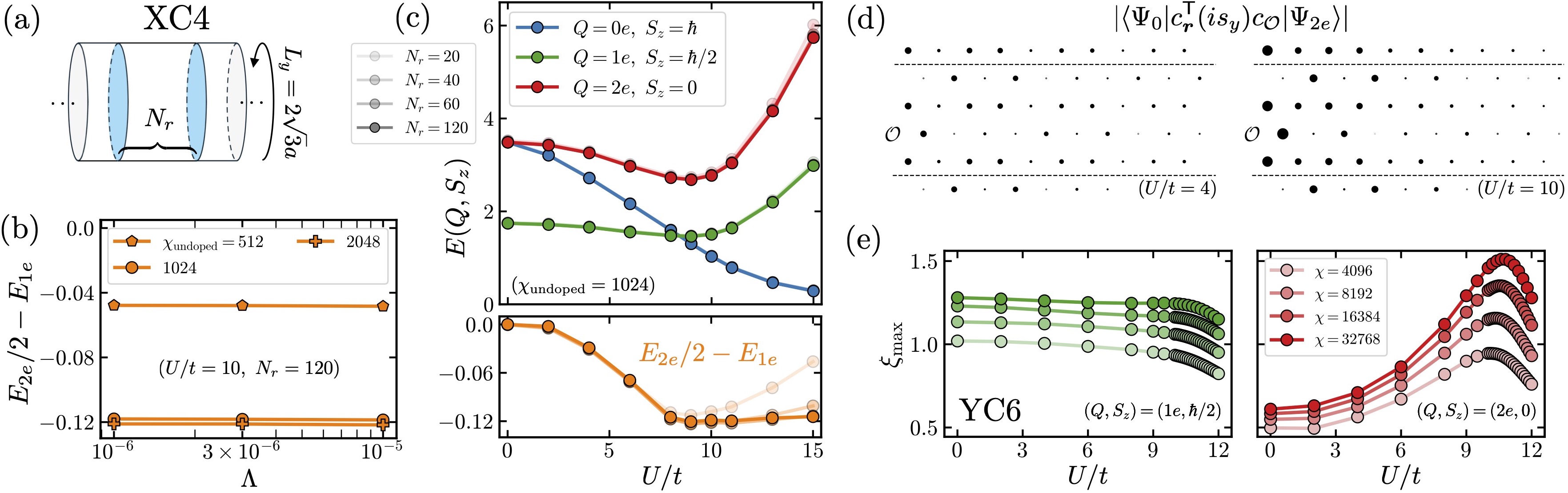
Figure 3: (a) Illustration of the infinite-length $\mathrm{XC}4$ cylinder with circumference $L_{y}=2\sqrt{3}a$, where $a$ is the lattice spacing. The “segment” DMRG method consists of optimizing a finite number of tensors (describing $N_{r}$ cylinder rings) sandwiched between two semi-infinite MPS environments derived from a reference (half-filled) ground state with bond dimension $\chi_{\mathrm{undoped}}$. (b) Electron pairing energy $E_{2e}/2-E_{1e}$ vs. maximum magnitude $\Lambda$ of discarded singular values in the finite segment, with legend indicating $\chi_{\mathrm{undoped}}$. (c) Upper panel: energies of excitations with charges $(Q,S_{z})$ (indicated in legend) vs. Hubbard $U$, with fixed $\chi_{\text{undoped}}=1024$ and $\Lambda=10^{-5}$. The legend indicates $N_{r}$ (increasing light to dark). Lower panel: electron pairing energy vs. $U$. (d) Magnitude of the pair wavefunction at both $U/t=4$ and $U/t=10$, computed from respective iDMRG ground states with $\chi_{\text{undoped}}=1024$ and segment excitations with $N_{r}=120$. The two dotted lines are related under the cylinder identification; outside points are periodic images. (e) Correlation lengths of the half-filled YC6 ground state in the $1e$ (left panel) and $2e$ (right) sectors, in units of cylinder rings, as a function of bond dimension (increasing light to dark) and $U$.

IV.2 Segment DMRG

Here we employ the “infinite boundary condition” technique [81, 82, 83, 84], referred to henceforth as the “segment” DMRG method [82, 85, 86], to obtain excited states and their energies. Starting from an infinite-MPS approximation to the ground state at half-filling, we allow the tensors of the excited-state MPS to differ on a segment spanning $N_{r}$ cylinder rings. DMRG is then used within this variational class to minimize the excitation energy for fixed quantum numbers $Q,S_{z}$, and circumferential momentum $k_{y}$ relative to the ground state.

For the XC4 cylinder considered here and shown schematically in Fig. 3(a), we identify points separated by $4\bm{a}_{2}-2\bm{a}_{1}\propto\hat{y}$ around the circumferential direction (with circumference $2\sqrt{3}a$), but take the cylinder to have infinite length, with $\bm{a}_{1}$ parallel to the cylinder axis. Each cylinder ring consists of two lattice sites. As in Ref. [39], we employ a gauge in which the magnetic unit cell consists of two sites, with magnetic Bravais vectors given by $\bm{a}_{1}$ and $2\bm{a}_{2}-\bm{a}_{1}.$ This results in two distinct momenta $k_{y}$, corresponding to the eigenvalues of the circumferential translation $(T_{2})^{2}T_{1}^{\dagger}$. To obtain the parent half-filled states, we use the iDMRG algorithm [87, 88], and conserve the charges $(Q,S_{z},k_{y})$ for both the ground state and the segment excitation calculations.

Accurate results require converging in three separate parameters: the bond dimension $\chi_{\mathrm{undoped}}$ of the half-filled ground state, the bond dimension of tensors within the variational segment—which we parameterize by the maximum magnitude $\Lambda$ of the discarded singular values—and the number of cylinder rings $N_{r}$ in the segment. In Fig. 3(b), we plot the pairing energy (for $U/t=10$ and $N_{r}=120$ rings) as a function of $\Lambda$ and parent state bond dimension. The energy is found to depend more strongly on the latter, but shows little quantitative difference between $\chi_{\mathrm{undoped}}=1024$ and $2048$, permitting us to choose the less expensive option at other interactions $U$. We focus on the XC4 cylinder because it is the largest system on which we can obtain $\lesssim 0.01t$ error in the energy using available resources, and because the smaller YC3 cylinder does not exhibit pairing, presumably due to insufficient cylinder width.

In Fig. 3(c), we plot the excitation energies in the charge sectors $(Q,S_{z})$ given by $\{(0e,\hbar),(1e,\hbar/2),(2e,0)\}$ as a function of Hubbard interaction $U$ and the segment length $N_{r}$ (increasing with shading, light to dark), fixing $\chi_{\text{undoped}}=1024$. For each $(Q,S_{z})$, we initialize in each momentum sector $k_{y}$ and take the minimum energy. We remark that the energy curves bear strong resemblance to those obtained from ED in Fig. 2(a). For the DMRG, we observe that the smaller-$U$ simulations exhibit more rapid energetic convergence in $N_{r}$. Both the $1e$ and $2e$ energies monotonically decrease from $U/t=0$ to a minimum at $U/t\approx 9$ and increase rapidly thereafter. Consistent with ED, their energies indicate electron pairing $E_{2e}/2-E_{1e}<0$ over a broad range of interaction strengths, from $U=0$ to at least $U/t=15$. The maximum pairing strength of $0.12t$ occurs at $U/t=9$ and constitutes $8.3\%$ of the corresponding $1e$ energy, though the data in fact exhibits a plateau in the pairing energy beginning at this $U$.

The behavior of the charge-neutral $S_{z}=\hbar$ excitation branch (see Fig. 3c) strongly resembles the corresponding energy curve in ED, where we identified it as belonging to a spin-triplet, pseudospin-singlet representation. In the segment DMRG data, this excitation energy decreases gradually from its expected value of $2\sqrt{3}t$ in the non-interacting limit to zero near $U/t\gtrsim 16$. This agrees quantitatively with the results from ED for both the $6\times 2$ and $4\times 4$-site systems, shown in Fig. 2(a), where this gap similarly closes at $U/t\gtrsim 15$. Agreement between these three geometries suggests this feature will persist to the thermodynamic limit, where it may be associated with a transition to the $120^{\circ}$ antiferromagnetic phase, setting an upper-bound on the extent of the putative CSL phase.

Though our explicit pairing calculations are limited to the XC$4$ cylinder, indirect evidence for the persistence and possible enhancement of pairing on wider cylinders is provided by the behavior of the transfer matrix spectrum associated with the translation-invariant half-filled parent state [38, 39]. The dominant transfer matrix eigenvalues, resolved by charge-sector $(Q,S_{z},k_{y})$, relate to ground-state connected correlation lengths of operators carrying those charges [89, 90]. In the $\text{YC-}L_{y}$ cylinder sequence [28], the correlation length associated with spin-singlet $2e$ excitations becomes more pronounced as $L_{y}$ increases from $L_{y}=3$ to $6$ (see App. D). In Fig. 3(e), we showcase the $2e$ and $1e$ correlation lengths on the YC6 cylinder, where the pronounced peak of $\xi_{2e}$ and its prominence over $\xi_{1e}$ suggests the persistence of electron pairing on this wider cylinder. The same pattern holds when comparing the $\text{XC}4$ and $\text{XC}6$ cylinders. In all cases, by threading flux if necessary, we ensure that the fluxes penetrating the cylinder rings are consistent with the particle-hole SO(4) symmetry of Sec. II.

IV.3 Pairing Symmetry

In this section, we discuss the symmetry of the charge-$2e$ paired states obtained in ED and DMRG. We argue that these states are energetically non-degenerate, spin-singlet, and carry odd angular momentum under site-centered rotation, but even angular momentum under bond-centered rotation.

On the $4\times 4$ system studied in ED, the uniqueness of the lowest-energy charge-$2e$ excited state for all $U$ implies that it is spin-singlet and transforms in a one-dimensional irreducible representation of the magnetic space group generated by $T_{1},C_{6}$. We find the pair carries momentum $T_{j}|\Psi_{2e}\rangle=-|\Psi_{2e}\rangle$ for all nearest-neighbour translations $T_{j}$. Counterintuitively, this is in fact the unique momentum which is rotation-symmetric: invariance under $C_{6}$ requires each $T_{j}$ to have the same eigenvalue, while Eq. (4) requires $T_{5}T_{3}T_{1}=-1$ when acting on a pair, which together implies $T_{j}=-1$. Moreover, we find that $C_{2}|\Psi_{2e}\rangle=-|\Psi_{2e}\rangle$, so that the state has odd angular momentum with respect to site-centered rotations. However, for each bond-centered rotation $C^{\mathrm{bond}}_{2}=T_{j}{C}_{2}$, we therefore have $C^{\mathrm{bond}}_{2}|\Psi_{2e}\rangle=+|\Psi_{2e}\rangle$, which has invariant meaning since $(C^{\mathrm{bond}}_{2})^{2}=1$ in every fermion-number sector. Thus, the pair has even angular momentum with respect to bond-centered rotations .

By anti-symmetry of the wavefunction, spin-singlet pairing should therefore be allowed between sites related by $C^{\mathrm{bond}}_{2}$ but disallowed when they are related by a site-centered rotation $C^{\mathrm{site}}_{2}$. This is exactly borne out in the $4\times 4$ ED numerical data. In Fig. 2(d), we plot the spin-singlet “pair wavefunction” $\langle\Psi_{0}|c^{\mathsf{T}}_{\bm{r}}(is_{y})c_{\mathcal{O}}|\Psi_{2e}\rangle$ at $U/t=6$, where $\Psi_{0}$ is the ground state and $\mathcal{O}$ is the origin. We observe that the wavefunction vanishes when $\bm{r}$ is related to $\mathcal{O}$ by some $C^{\mathrm{site}}_{2}$, in agreement with the above arguments. Moreover, the pair is well-localized, with nearest-neighbour pairing having much larger magnitude than next-nearest-neighbour pairing. Though the phase winding in Fig. 2(d) suggests the pairing symmetry is “$p+ip$”, we caution that the $C_{3}$ eigenvalue of the charge-$2e$ excited state does not have obvious invariant meaning as it can be modified by the redefinition $C_{3}\to e^{2\pi i/3}C_{3}$. Nonetheless, on the $4\times 4$ torus, we have unambiguously confirmed spin-singlet pairing, carrying odd angular momentum under site-centered rotations and even angular momentum under bond-centered rotations.

On the XC4 cylinder, three-fold rotation symmetry is explicitly broken. Nonetheless, the segment DMRG pair excitations exhibit the same pairing symmetry as above. We verify this explicitly by computing the pair wavefunction, choosing $\mathcal{O}$ at the center of the segment . We find it is odd under $\bm{r}\to C_{2}\bm{r}$ and that the spin-triplet overlap is several orders of magnitude smaller than spin-singlet. Moreover, as shown in Fig. 3(d) for $U/t=4$ and $10$, we find that the pair wavefunction vanishes approximately (error induced by finite $N_{r}$) when $\bm{r}$ and $\mathcal{O}$ are related by some ${C}^{\text{site}}_{2}$, which indicates ${C}^{\text{site}}_{2}|\Psi_{2e}\rangle=-|\Psi_{2e}\rangle$. Similarly, we conclude that ${C}^{\text{bond}}_{2}|\Psi_{2e}\rangle=+|\Psi_{2e}\rangle$. These plots also show that the size of the excitation decreases with $U$. Finally, since we conserve momentum around the cylinder, our excited states are labeled by their eigenvalue under the circumferential translation ${T}=(T_{2})^{2}T_{1}^{\dagger}$. For all $U$, the paired eigenstate satisfies ${T}|\Psi_{2e}\rangle=-|\Psi_{2e}\rangle$, consistent with our expectation $T_{1}=T_{2}=-1$.

We anticipate that our pairing symmetry results will help guide future numerical investigations of pairing and superconductivity in this model, especially those employing techniques that operate within a fixed charge sector, such as the ED and DMRG performed in this work.

IV.4 Pairing at the conduction band edge

Both our ED (Fig. 2) and DMRG (Fig. 3) numerics indicate that pairing extends down to infinitesimal values of $U$. Though our discussion has focused largely on the intermediate-coupling regime near topological criticality, the regime of perturbatively-weak interactions allows for an independent check of the existence and symmetry of bound pairs in our model, which we fix here to be spin-singlet. To second order in many-body perturbation theory, renormalization of the two-body scattering vertex is described by the following five diagrams [93, 94, 95]:

$$\leavevmode\hbox to34.54pt{\vbox to23.16pt{\text{[drawing]}}},\,\leavevmode\hbox to34.54pt{\vbox to24.09pt{\text{[drawing]}}},\,\leavevmode\hbox to34.54pt{\vbox to25.66pt{\text{[drawing]}}},\,\leavevmode\hbox to34.54pt{\vbox to25.66pt{\text{[drawing]}}},\,\leavevmode\hbox to34.54pt{\vbox to23.16pt{\text{[drawing]}}}$$ (14)

where curvy and straight lines denote interaction events and single-particle propagators, respectively. As shown in Ref. [96] in the context of superconductivity mediated by local repulsion [97, 98], some of these diagrams vanish given a specific bare interaction kernel. For our model at half filling and zero temperature, we show in App. G that only the “cross” diagram contributes to the Cooper vertex in the spin-singlet channel at zero temperature and charge neutrality. Restricting our attention to the four degenerate single-particle states at the conduction band edge, labeled by their momenta $\kappa,\kappa^{\prime}$ and degenerate band index $n\in\{1,2\}$ (see Fig. 1c), we find that this diagram only mediates pairing in the channel:

$$\hat{\Delta} =c_{\kappa^{\prime},\uparrow,2}c_{\kappa,\downarrow,1}-c_{\kappa^{\prime},\downarrow,2}c_{\kappa,\uparrow,1}$$ (15)

$$\qquad-c_{\kappa,\uparrow,2}c_{\kappa^{\prime},\downarrow,1}+c_{\kappa,\downarrow,2}c_{\kappa^{\prime},\uparrow,1}.$$

Consistent with our ED and DMRG, this spin-singlet pair has odd angular momentum with respect to site-centered rotations.

V Discussion

A central and broad message of this work is that topological superconductivity can emerge in a regime with both strong repulsive interactions and broken time reversal symmetry. Electron pairing was investigated and was clearly observed in our numerical calculations on the present Hofstadter-Hubbard model. The pairs are spin-singlet, carrying odd angular momentum under site-centered rotations and even angular momentum under bond-centered rotations. Moreover, the pairing energy was found to be largest in the vicinity of the critical point, decreasing—but remarkably remaining finite—down to perturbatively-weak interactions.

These numerical observations are consistent with, and were in fact inspired by, the central idea that proximity to topological quantum criticality can offer a robust route to superconductivity, even in remarkably simple settings. The crucial ingredient here is that the topological transition is associated with the closing of the charge gap, while the spin gap remains open. For the IQH-CSL critical theory in the Hofstadter-Hubbard model, we argued that doping naturally leads to a topological superconductor. On the CSL side of the phase diagram, this relates to the storied mechanism of semion superconductivity. However, given the broad extent around criticality where superconductivity is anticipated, it is not strictly necessary for this mechanism that the topological critical point or the CSL be accessed in a given model. For instance, superconductivity could emerge upon doping the IQH well away from criticality, even in a scenario where the CSL is entirely subsumed by a conventional antiferromagnetic phase, or if the transition exists but is weakly first-order. For the same reason, we do not expect $C_{2}$-breaking or deviation from particle-hole symmetry to play a significant role away from weak coupling, although quantifying their effects is an excellent topic for future research.

Let us list some other key areas for future exploration. An immediate next step is numerically verifying the existence of a superconducting ground state at non-vanishing doping in this model. Furthermore, to distinguish features unique to the specific model from those of the general theoretical scenario near the critical point, it will be necessary to compare results for a broader class of models that relax various symmetries enjoyed by the present model. Such results should also be compared to numerical observations of superconductivity in related models on the triangular lattice [99], most notably chiral $t$-$J$ models with real hoppings [100, 101, 102, 103], where the charge fluctuations integral to topological criticality are absent.

Next, we highlight promising experimental realizations in moiré materials. Triangular lattices formed by TMD sheets with a superimposed moiré potential offer both valley and layer-pseudospin degrees of freedom [104, 105, 106, 107, 108, 109]. As proposed in prior work [40, 38], the Hofstadter-Hubbard model considered here could be realized by applying a magnetic field whose strength is made feasible by the tens-of-nanometer moiré spacing. This field would conveniently polarize the valley degree of freedom, yielding an SU(2) layer-pseudospin-symmetric effective model [38]. Further numerical studies of this model would help guide the experimental exploration of criticality and superconductivity in these platforms.

Finally, the recent experimental observation of the fractional quantum anomalous Hall effect in twisted bilayer $\mathrm{MoTe}_{2}$ [110, 111, 112, 113] and rhombohedral multilayer graphene [114], as well as fractional Chern insulators in both magic-angle graphene at weak magnetic field [115] and in the field-induced Chern bands of bernal-bilayer graphene aligned with hexagonal boron nitride [116], compel us to explore the behavior of charged anyons subject to substantial lattice effects, as we have in this work. Furthermore, a recent experiment on quadrilayer rhombohedral graphene demonstrates that chiral superconductivity is possible even at strong magnetic fields [117], a hopeful sign for the class of mechanisms considered here, motivating the study of routes to pairing and superconductivity in the strong time-reversal-breaking regime.

oneΔ

Supplementary Material: “Anyon Superconductivity from Topological Criticality in a Hofstadter-Hubbard Model”

Appendix A Coordinates and different gauge choices

SI Triangular lattice coordinates

Here, we specify the Bravais vectors of the underlying triangular lattice (see Fig. 1b):

$$\bm{a}_{1}=\hat{x},\qquad\bm{a}_{2}=\frac{\hat{x}}{2}+\frac{\hat{y}\sqrt{3}}{2}$$ (1)

where we’ve set the nearest-neighbour lattice bond length to unity, $a=1$. The lattice points are then given by

$$\bm{r}=n_{1}\bm{a}_{1}+n_{2}\bm{a}_{2},\qquad n_{i}\in\mathbb{Z},$$ (2)

We take the reciprocal lattice vectors to be

$$\bm{b}_{1}=2\pi\hat{x}-\frac{2\pi}{\sqrt{3}}\hat{y},\qquad\bm{b}_{2}=\frac{4\pi}{\sqrt{3}}\hat{y}.$$ (3)

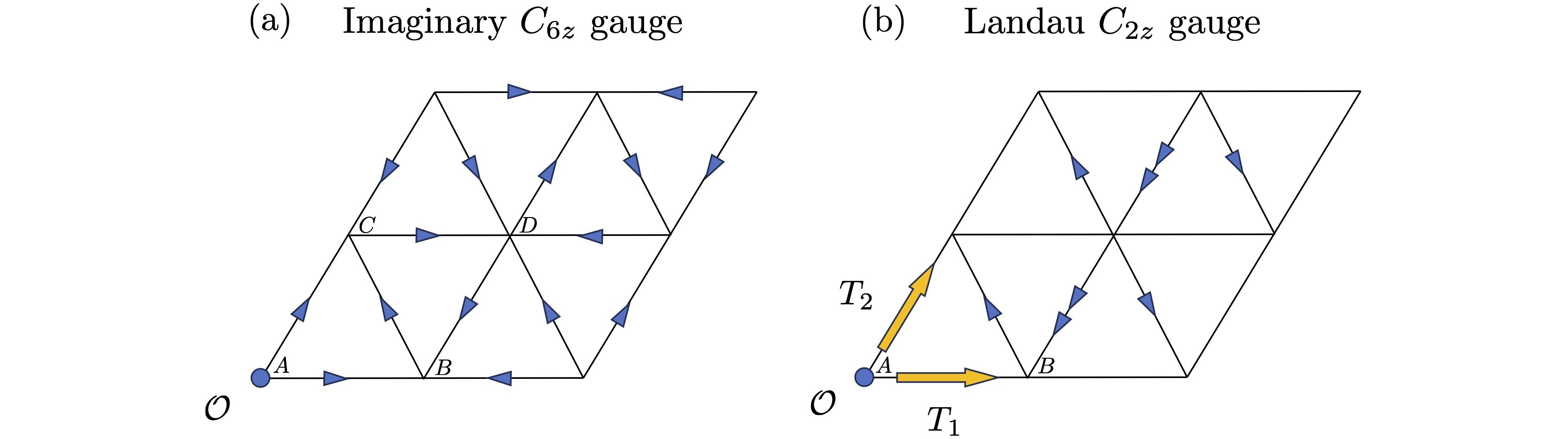
Figure A1: Two possible gauges for the hopping Hamiltonian, in both cases giving rise to $\Phi_{\triangle}=\pi/2$ magnetic flux per triangular plaquette. (a) Hoppings in the “Imaginary $C_{6}$” gauge, which is manifestly $C_{6}$ symmetric about the origin [bottom left marked by $\mathcal{O}$]. The origin is chosen to coincide with the $A$ sublattice (other sublattices $B,C,D$ are also marked). Each arrow indicates a Peirel’s phase of $+i$ in the direction of the arrow. This gauge chose is identical to that displayed in Fig. 1(b) of the main text, except there the origin is in the middle of the image. (b) Hoppings in the “Landau $C_{2}$” gauge. All hoppings are either imaginary or real, with a single arrow again indicating a Peirel’s phase of $+i$ in the direction of the arrow. $T_{1}$ and $T_{2}$ (yellow arrows) denote translation symmetry in the unit directions $\bm{a}_{1}$ and $\bm{a}_{2}$, respectively. The forms of $T_{1,2}$ is different in the two gauges and are given in App. A.

SII Imaginary $C_{6}$ gauge

Fig. A1(a) provides an electronic gauge in which the hoppings are purely imaginary and in which the $C_{6}$ symmetry acts in its bare form in real space:

$$C_{6}c^{\dagger}_{\bm{r}}C_{6}^{-1}=c^{\dagger}_{C_{6}\bm{r}},$$ (4)

provided that the (infinite 2D or torus) geometry is such that $C_{6}$ is well-defined. For the torus, this means that the equivalence class of identified points faithfully maps to an equivalence class of identified points. This can easily be seen to fail for a $4\times 2$ size torus, for example.

By inspecting the phases of the hoppings in Fig. A1(a), we read off

$$T_{1}c^{\dagger}_{\bm{r}}T_{1}^{-1}=i(-1)^{n_{1}+n_{2}}c^{\dagger}_{\bm{r}+\bm{a}_{1}},\qquad T_{2}c^{\dagger}_{\bm{r}}T_{2}^{-1}=i(-1)^{n_{2}}c^{\dagger}_{\bm{r}+\bm{a}_{2}}.$$ (5)

To see the former, note that only the hoppings parallel to $\bm{a}_{1}-\bm{a}_{2}$ are left invariant by bare $T_{1}$, i.e. the hoppings in the $\bm{a}_{1}$ and $\bm{a}_{2}$ directions pick up a minus sign that needs to be corrected. For the latter, bare $T_{2}$ instead negates the hoppings in the $\bm{a}_{2}$ and $\bm{a}_{1}-\bm{a}_{2}$ directions. The factors $i$ are chosen so that two-fold translation is a pure shift:

$$(T_{j})^{2}c_{\bm{r}}^{\dagger}(T_{j})^{-2}=c_{\bm{r}+2\bm{a}_{j}}^{\dagger}.$$ (6)

But more importantly, the definitions Eq. (4) and Eq. (5) are chosen to be consistent with all the algebraic conditions laid out in Sec. II of the main text.

As a non-trivial check of correctness of these translations, we can show that they correctly anti-commute:

$$(T_{1}\circ T_{2})\cdot c^{\dagger}_{\bm{r}} =-T_{1}T_{2}c^{\dagger}_{\bm{r}}T_{2}^{-1}T_{1}^{-1}$$ (7)

$$=-(-1)^{n_{2}}T_{1}c^{\dagger}_{\bm{r}+\bm{a}_{2}}T_{1}^{-1}$$ (8)

$$=(-1)^{n_{2}}(-1)^{n_{1}+n_{2}}c^{\dagger}_{\bm{r}+\bm{a}_{2}+\bm{a}_{1}}$$ (9)

compared to

$$(T_{2}\circ T_{1})\cdot c^{\dagger}_{\bm{r}} =-T_{2}T_{1}c^{\dagger}_{\bm{r}}T_{1}^{-1}T_{2}^{-1}$$ (10)

$$=-(-1)^{n_{1}+n_{2}}T_{2}c^{\dagger}_{\bm{r}+\bm{a}_{1}}T_{2}^{-1}$$ (11)

$$=-(-1)^{n_{1}+n_{2}}(-1)^{n_{2}}c^{\dagger}_{\bm{r}+\bm{a}_{1}+\bm{a}_{2}},$$ (12)

so that indeed $T_{2}T_{1}=(-1)^{N_{F}}T_{1}T_{2}$.

The phases can be written in a more geometric form:

$$T_{1}c^{\dagger}_{\bm{r}}T_{1}^{\dagger}=ie^{i\bm{r}\cdot(\bm{b}_{1}+\bm{b}_{2})/2}c^{\dagger}_{\bm{r}+\bm{a}_{1}},\qquad T_{2}c^{\dagger}_{\bm{r}}T_{2}^{\dagger}=ie^{i\bm{r}\cdot\bm{b}_{2}/2}c^{\dagger}_{\bm{r}+\bm{a}_{2}}.$$ (13)

From these, we can also obtain

$$(T_{1}^{\dagger}T_{2})c_{\bm{r}}^{\dagger}(T_{1}^{\dagger}T_{2})^{\dagger}=e^{-i\bm{r}\cdot\bm{b}_{1}/2}c_{\bm{r}-\bm{a}_{1}+\bm{a}_{2}}^{\dagger},$$ (14)

and by inverting the above three,

$$T_{1}^{\dagger}c_{\bm{r}}^{\dagger}T_{1} =ie^{-i\bm{r}\cdot(\bm{b}_{1}+\bm{b}_{2})/2}c_{\bm{r}-\bm{a}_{1}}^{\dagger}$$ (15)

$$T_{2}^{\dagger}c_{\bm{r}}^{\dagger}T_{2} =ie^{-i\bm{r}\cdot\bm{b}_{2}/2}c_{\bm{r}-\bm{a}_{2}}^{\dagger}$$ (16)

$$(T_{1}^{\dagger}T_{2})^{\dagger}c_{\bm{r}}^{\dagger}(T_{1}^{\dagger}T_{2}) =-e^{i\bm{r}\cdot\bm{b}_{1}/2}c_{\bm{r}+\bm{a}_{1}-\bm{a}_{2}}^{\dagger}.$$ (17)

From this we learn that $C_{6}T_{1}C_{6}^{\dagger}=T_{2}$:

$$(C_{6}T_{1}C_{6}^{\dagger})c_{\bm{r}}^{\dagger}(C_{6}T_{1}C_{6}^{\dagger})^{\dagger} =(C_{6}T_{1})c_{C_{6}^{-1}\bm{r}}^{\dagger}(C_{6}T_{1})^{\dagger}$$ (18)

$$=iC_{6}e^{iC_{6}^{-1}\bm{r}\cdot(\bm{b}_{1}+\bm{b}_{2})/2}c_{C_{6}^{-1}\bm{r}+\bm{a}_{1}}^{\dagger}C_{6}^{\dagger}$$ (19)

$$=ie^{i\bm{r}\cdot C_{6}(\bm{b}_{1}+\bm{b}_{2})/2}c_{\bm{r}+C_{6}\bm{a}_{1}}^{\dagger}$$ (20)

$$=ie^{i\bm{r}\cdot\bm{b}_{2}/2}c_{\bm{r}+\bm{a}_{2}}^{\dagger}$$ (21)

$$=T_{2}c_{\bm{r}}^{\dagger}T_{2}^{\dagger}.$$ (22)

Similarly, it can be shown that $T_{3}=C_{6}T_{2}C_{6}^{\dagger}=(-i)^{N_{F}}T_{1}^{\dagger}T_{2}$ and $C_{6}T_{3}C_{6}^{\dagger}=T_{1}^{\dagger},$ which is altogether consistent with $C_{2}T_{j}C_{2}=(T_{j})^{\dagger}$ for all $j$.

Closed-form composition of translation generators

Here we provide the closed form expression for powers of $T_{1}$ and $T_{2},$ namely

$$T_{2}^{M}c_{\bm{r}}^{\dagger}T_{2}^{-M} =i^{M}c_{\bm{r}+M\bm{a}_{2}}^{\dagger}\prod_{j=0}^{M-1}e^{i(\bm{r}+j\bm{a}_{2})\cdot\bm{b}_{2}/2}$$ (23)

$$=i^{M}c_{\bm{r}+M\bm{a}_{2}}^{\dagger}e^{i\sum_{j=0}^{M-1}\bm{r}\cdot\bm{b}_{2}/2}e^{i\pi\sum_{j=0}^{M-1}j}$$ (24)

$$=i^{M}c_{\bm{r}+M\bm{a}_{2}}^{\dagger}e^{iM\bm{r}\cdot\bm{b}_{2}/2}e^{i\pi M(M-1)/2}$$ (25)

$$=c_{\bm{r}+M\bm{a}_{2}}^{\dagger}e^{iM\bm{r}\cdot\bm{b}_{2}/2}e^{i\pi M^{2}/2},$$ (26)

and similarly

$$T_{1}^{M}c_{\bm{r}}^{\dagger}T_{1}^{-M} =i^{M}c_{\bm{r}+M\bm{a}_{1}}^{\dagger}\prod_{j=0}^{M-1}e^{i(\bm{r}+j\bm{a}_{2})\cdot(\bm{b}_{1}+\bm{b}_{2})/2}$$ (27)

$$=i^{M}c_{\bm{r}+M\bm{a}_{1}}^{\dagger}e^{iM\bm{r}\cdot(\bm{b}_{1}+\bm{b}_{2})/2}e^{i\pi M(M-1)/2}$$ (28)

$$=c_{\bm{r}+M\bm{a}_{1}}^{\dagger}e^{iM\bm{r}\cdot(\bm{b}_{1}+\bm{b}_{2})/2}e^{i\pi M^{2}/2}.$$ (29)

Then for two-electron operators, in particular, we obtain:

$$T_{\bm{M}}c_{\bm{r}}^{\dagger}c_{\bm{r}^{\prime}}^{\dagger}T_{\bm{M}}^{\dagger} =T_{2}^{M_{2}}T_{1}^{M_{1}}c_{\bm{r}}^{\dagger}c_{\bm{r}^{\prime}}^{\dagger}T_{1}^{-M_{1}}T_{2}^{-M_{2}}$$ (30)

$$=e^{i\pi M_{1}^{2}}e^{iM_{1}(\bm{r}+\bm{r}^{\prime})\cdot(\bm{b}_{1}+\bm{b}_{2})/2}T_{2}^{M_{2}}c_{\bm{r}+M_{1}\bm{a}_{1}}^{\dagger}c_{\bm{r}^{\prime}+M_{1}\bm{a}_{1}}^{\dagger}T_{2}^{-M_{2}}$$ (31)

$$=e^{i\pi(M_{1}^{2}+M_{2}^{2})}e^{iM_{1}(\bm{r}+\bm{r}^{\prime})\cdot(\bm{b}_{1}+\bm{b}_{2})/2}e^{iM_{2}(\bm{r}+M_{1}\bm{a}_{1})\cdot\bm{b}_{2}/2}e^{iM_{2}(\bm{r}^{\prime}+M_{1}\bm{a}_{1})\cdot\bm{b}_{2}/2}c_{\bm{r}+\bm{M}}^{\dagger}c_{\bm{r}^{\prime}+\bm{M}}^{\dagger}$$ (32)

$$=e^{i\pi(M_{1}^{2}+M_{2}^{2})}e^{iM_{1}(\bm{r}+\bm{r}^{\prime})\cdot(\bm{b}_{1}+\bm{b}_{2})/2}e^{iM_{2}\bm{r}\cdot\bm{b}_{2}/2}e^{iM_{2}\bm{r}^{\prime}\cdot\bm{b}_{2}/2}c_{\bm{r}+\bm{M}}^{\dagger}c_{\bm{r}^{\prime}+\bm{M}}^{\dagger}.$$ (33)

Appendix B Details of the U(1) Slave Rotor Theory and a Mean Field Estimate of the Transition

We utilize the slave-rotor approach [56, 124], introducing a U(1) rotor variable $e^{i\theta}$ and its conjugate integer-valued “angular momentum” $L$ on each site and writing the electron operator as

$$c^{\dagger}_{i,\sigma}=f^{\dagger}_{i,\sigma}\,e^{i\theta_{i}},$$ (34)

where $f_{\sigma}$ is a fermionic “spinon” that carries the spin index. The Hilbert space redundancy introduced by the rotors is removed by requiring that each site satisfy a constraint:

$$L_{i}=\sum_{\sigma}\left(f^{\dagger}_{i,\sigma}f_{i,\sigma}-1/2\right)$$ (35)

Note that the singly-filled site is represented by $L_{i}=0$, while the doublon/empty sites are $L_{i}=\pm 1$. The Hubbard model can then be rewritten as:

$$H=-\sum_{\langle ij\rangle,\sigma}t_{ij}e^{i(\theta_{i}-\theta_{j})}f^{\dagger}_{i,\sigma}f_{j,\sigma}+{\rm h.c.}+\frac{U}{2}\sum_{i}L_{i}^{2},$$ (36)

supplemented with the constraint Eq. (35) and the commutation relation $\left[e^{i\theta_{i}},\,L_{j}\right]=-\delta_{ij}e^{i\theta_{i}}$.

Of course, treating everything exactly is tantamount to solving the original problem, but we can make progress by adopting a mean field approach, satisfying the constraint on average and assigning self-consistent expectation values to $\langle f^{\dagger}_{i,\sigma}f_{j,\sigma}\rangle$ and $\langle e^{i(\theta_{i}-\theta_{j})}\rangle$. This gives us the mean field Hamiltonian:

$$H_{MF} = H_{f}+H_{\theta}$$ (37)

$$H_{f} = -\sum_{\langle ij\rangle,\sigma}t_{ij}\langle e^{i(\theta_{i}-\theta_{j})}\rangle f^{\dagger}_{i,\sigma}f_{j,\sigma}+{\rm h.c.}$$ (38)

$$H_{\theta} = -\sum_{\langle ij\rangle,\sigma}t_{ij}e^{i(\theta_{i}-\theta_{j})}\langle f^{\dagger}_{i,\sigma}f_{j,\sigma}\rangle+{\rm h.c.}+\frac{U}{2}\sum_{i}L_{i}^{2}$$ (39)

Note that the constraint Eq. (35) implies gauge invariance, $\theta_{i}\rightarrow\theta_{i}+\epsilon_{i},\,f^{\dagger}_{i}\rightarrow f^{\dagger}_{i}e^{-i\epsilon_{i}}$ which is broken by the mean field Hamiltonian. This is remedied by incorporating a fluctuating gauge field $a$ on the links, though we shall not do that here.

In the limit of small Hubbard $U$, we expect the rotor fields to condense, $\langle e^{i\theta_{i}}\rangle=\sqrt{Z_{i}}\leq 1$, so that the spinons $f$ are identified with the electron up to this prefactor. This phase possesses off-diagonal long-range order; at the mean-field level, we assume $\langle e^{i(\theta_{i}-\theta_{j})}\rangle\approx\langle e^{i\theta_{i}}\rangle\langle e^{-i\theta_{j}}\rangle$. Thus, the gap to the electron excitation is obtained from the dispersion $t_{ij}\sqrt{Z_{i}Z_{j}}f^{\dagger}_{i}f_{j}$, which explains why the single-electron gap on the IQH side (i.e., the condensed rotor phase) decreases on increasing $U$.

On the other side of the phase diagram, when $U$ is sufficiently large, we have $\langle e^{i\theta_{i}}\rangle=0$ and thus the electron excitation is distinct from the spinon. To create an electron, one must both create a spinon $f^{\dagger}$ and increase the rotor angular momentum by $\Delta L=1$. Thus, due to the interaction term, this gap tracks $U$ for large $U$. Despite the absence of an expectation value $\langle e^{i\theta_{i}}\rangle=0$ on this side, there is virtual tunneling of the rotor quanta, so that $\langle e^{i(\theta_{i}-\theta_{j})}\rangle=\beta_{ij}\neq 0$ for neighboring sites [125]. In fact, this expectation value is expected to scale as $|t|/U$, in the large $U$ limit, implying that the dispersion of spinons in Eq. (39) is on the order of $t^{2}/U$, as is expected of magnetic excitations. On the other hand, if we assume that the expectation values $\beta_{ij}$ are positive, consistent with the fact that the rotors see no net flux (while the electrons and spinons do), then we simply fill up the negative energy states of the band-structure shown in Fig. 1(c), albeit with a smaller gap. This gives a non-zero value for the rotor hoppings, $\langle f^{\dagger}_{i,\sigma}f_{j,\sigma}\rangle=\alpha_{ij}$. We can find this expectation value from the ground state energy of the band Hamiltonian: writing $\alpha_{ij}=-t^{*}_{ij}\alpha/|t|$, we expect the average over the filled bands $\langle\epsilon^{-}(k)\rangle$ to determine $\alpha=\frac{|\langle\epsilon^{-}(k)\rangle|}{2z|t|}$, where $z=6$ is the coordination number.

Now we can determine the transition, which amounts to analyzing the Bose-Hubbard model

$$H_{B}=-J\sum_{\langle ij\rangle}e^{i(\theta_{i}-\theta_{j})}+{\rm h.c.}+\frac{U}{2}\sum_{i}L_{i}^{2}.$$ (40)

A simple mean field theory locates the transition at $U^{*}=4zJ$. This is done by taking a simple variational ansatz for each site, $|\psi\rangle=|0\rangle+\frac{\psi}{2}\left(|+1\rangle+|-1\rangle\right)$ in the $L$ basis, which has the property $\langle\psi|e^{i\theta}|\psi\rangle=\psi$. Then $\langle H_{B}\rangle=N\psi^{2}(-zJ+\frac{U}{4})$. The condensate occurs when the coefficient in parentheses first turns negative.

Substituting $J=2|t|\alpha$, where the factor of $2$ is for the two spins of $f$, we get:

$$U^{*}=4|\langle\epsilon^{-}(k)\rangle|\approx 9.60813\,t$$ (41)

where we averaged over the dispersion $\epsilon_{-}(k)=-2t\sqrt{\cos^{2}k_{1}+\cos^{2}k_{2}+\cos^{2}(k_{1}+k_{2})}$. This mean field result is to be compared to, and is indeed relatively close to, the numerically-obtained transition at $U^{*}\approx 12t$ [38, 39].

Additionally, we can argue directly that the gap to the charge-$2e$ Cooper pair excitations vanishes at the transition. To access them one has to include coupling to the internal gauge field $a$. If we focus on the transition and integrate out the fermionic spinons $f$, this gives a Chern-Simons term [60]. Also, the rotor variables are at low energies and couple minimally to the gauge field. In the condensed phase of the rotors, we have the effective Lagrangian:

$$L=\frac{1}{4U}\left(\dot{\theta}-a_{0}\right)^{2}-\frac{\rho_{s}}{2}\left(\nabla{\theta}-a\right)^{2}-\frac{2}{4\pi}a\wedge da,$$ (42)

where the superfluid density $\rho_{s}$ goes to zero at the transition. The vortices of the rotor condensate are the Cooper pairs. The fact that they carry $2\pi$ flux of $da$ implies, via the Chern-Simons term, a gauge charge of $2$. This is screened by two rotor fields, giving the vortex a global $\mathrm{U(1)}_{c}$ charge of $2$ and no spin. The energy of such vortices vanishes as we approach the transition.

Appendix C Chirality of Edge States from K-Matrix Formalism

We note that the edge chiral central charge on the IQHE side is $c_{-}=2$ while on the CSL side it is $c_{-}=1$ [126, 127]. Also, in the superconductor we expect $c_{-}=2$. In this section, we derive these from the effective field theory for these phases and confirm these expectations.

Consider a multi-component Chern Simons theory ${\mathcal{L}}=\frac{K_{IJ}}{4\pi}a_{I}da_{J}$, where we have dispensed with the wedge symbol. A key point is that the number of positive minus the number of negative eigenvalues of the $K$ matrix corresponds to the edge state chirality $c_{-}$, i.e., the number of (say) right mover minus left movers at the edge (this is clear by looking at the edge states associated with the $K$ matrix) [69, 71]. Furthermore, $|{\rm det}\,K|$ reflects the ground state degeneracy on the torus, or equivalently, the number of distinct anyon types [128].

First, the IQHE is represented by the free fermion theory, which can be written as ${\mathcal{L}}_{I}=\frac{1}{4\pi}\beta_{1}d\beta_{1}+\frac{1}{4\pi}\beta_{2}d\beta_{2}$ (one term for each spin species), which has $K=\begin{bmatrix}1&0\\ 0&1\end{bmatrix}$ and thus $c_{-}=2$.

To obtain the CSL, we must couple these to a gauge field $a$ via ${\mathcal{L}}_{I}=\frac{1}{4\pi}\beta_{1}d\beta_{1}+\frac{1}{4\pi}\beta_{2}d\beta_{2}+\frac{2}{4\pi}(\beta_{1}+\beta_{2})da$, which gives the following $K$ matrix:

$$K_{\mathrm{II}}=\begin{bmatrix}0&1&1\\ 1&1&0\\ 1&0&1\end{bmatrix}.$$ (43)

We find that it has $\det K=-2$, as expected for the CSL, which has a two-fold ground state degeneracy on the torus. Also, its eigenvalues are $\{2,\,-1,\,1\}$, which corresponds to a single right mover, i.e., $c_{-}=1$.

Now, let us turn to the anyon superconductor and the chirality of its edge modes. From the main text, recall that the main additional step was that the gauge field $a$ now has a bIQH response with $\frac{2}{4\pi}ada$. This gives the $K$ matrix:

$$K_{\rm doped}=\begin{bmatrix}2&1&1\\ 1&1&0\\ 1&0&1\end{bmatrix},$$ (44)

for which we find that ${\rm\det}\,K=0$. The fact that it vanishes indicates broken symmetry, i.e., a superconductor. We would like to know how many chiral modes the superconductor has.

One way to proceed is to examine the Chern-Simons Lagrangian more closely which, after collecting terms, can be written as ${\mathcal{L}}_{\rm doped}=\frac{1}{4\pi}(\beta_{1}+a)d(\beta_{1}+a)+\frac{1}{4\pi}(\beta_{2}+a)d(\beta_{2}+a).$ Clearly, we can absorb $a$ into $\beta_{1},\,\beta_{2}$ which gives rise to the zero eigenvalue, and confirms that these fields are not independent (signaled by ${\rm\det}\,K=0$). What is left are the two chiral modes of the topological superfluid.

Another approach is to promote to a dynamical variable the probe gauge field $A$ that couples to the global charge U(1). This will remove the gapless Goldstone mode of the superfluid and give rise to topological order—one of the Kitaev 16-fold way $\mathbb{Z}_{2}$ topological orders [69]—that can help us identify the nature of edge states in the original superfluid. For example, a topologically-trivial superfluid would lead to toric code topological order, i.e., the $m=0$ member of the 16-fold way. In fact, we only expect one of the 8 even members of the 16-fold way since we will only describe Abelian topological orders via the $K$ matrix.

Since $A$ couples to the chargons, it appears in the $\frac{2}{4\pi}(a-A)d(a-A)$ term originating from the chargon bIQH phase. However, it is convenient here to redefine $\tilde{a}=a-A$ and then, for notational simplicity, relabel $\tilde{a}\rightarrow a$. Adding together all terms in $K_{\rm doped}$ along with this coupling to $A$, we find:

$${\mathcal{L}}_{\rm doped\text{-}gauged}=\frac{2}{4\pi}ada+\frac{1}{4\pi}\beta_{1}d\beta_{1}+\frac{1}{4\pi}\beta_{2}d\beta_{2}+\frac{1}{2\pi}(a+A)(d\beta_{1}+d\beta_{2}).$$ (45)

Note that the implication of gauging the global charge U(1) is that we treat $A$ as a dynamical field and can integrate it out. This pins $\beta_{1}=-\beta_{2}$ and yields the effective Lagrangian ${\mathcal{L}}_{\rm doped\text{-}gauged}=\frac{2}{4\pi}ada+\frac{2}{4\pi}\beta_{1}d\beta_{1}$, corresponding to:

$$K_{\mathrm{doped\text{-}gauged}}=\begin{bmatrix}2&0\\ 0&2\end{bmatrix}.$$ (46)

This corresponds to two copies of semion topological order, with anyons $\{1,\,s_{1},\,s_{2},\,f=s_{1}s_{2}\}$, where the composite of the two semions is a fermion. Note that ${\rm\det}\,K_{\mathrm{doped\text{-}gauged}}=4$ and $c_{-}=2$, which corresponds to the member $m=4$ of the 16-fold way [69]. This implies that the edge state content of the original superfluid is $c_{-}=2\ \rm{mod\ 8}$, consistent with the topology of “$d+id$” weak-pairing superconductors [61]. However, recall from the main text that our superconductor is far from the weak-pairing limit, so that its pairing symmetry is not directly linked to its chiral central charge.

Appendix D Correlation Lengths at Half-Filling from Cylinder iDMRG

In this section, we provide the transfer matrix correlation length data for the ground states at half-filling, for a range of Hubbard interaction strengths $U$ and various system sizes. We consider both the YC-$L_{y}$ and XC-$2L_{y}$ cylinder geometries [28]. We adopt the electronic gauge and conventions of Ref. [39]. Rephrased in the more gauge-invariant language of Sec. II of the main text, in the YC case with even $L_{y}$, we take $T=T_{2}$ to be a purely circumferential translation with $T^{L_{y}}=1$. When $L_{y}$ is odd, we instead thread $\pi/2$ flux so that $T^{L_{y}}=i^{N_{F}}$, which means that $T$ can have eigenvalue $-1$ in the charge-$2e$ $(N_{F}=2)$ sector. The XC case proceeds the same way except that we take our circumferential translation to be $T=(T_{2})^{2}T_{1}^{\dagger}$, which translates by a distance $\sqrt{3}a$ instead of $a$.

The dominant correlation length $\xi$ in a given charge sector of the transfer matrix is related to the dominant non-trivial transfer matrix eigenvalue $\lambda$ by [89]:

$$1/\xi_{i}=-\log\left|\lambda_{i}\right|$$ (47)

We report $\xi$ in units of cylinder rings. For the YC cylinders, the distance between the cylinder rings is $a\sqrt{3}/2$, whereas it is $a/2$ in the XC case.

In Fig. A2, we display the maximum correlation lengths for the YC3, YC4 and YC6 cylinders resolved by the electric charge sector of the ground state transfer matrix, namely $Q\in\{0e,1e,2e\}$, where we maximize over spin and momentum quantum numbers for simplicity of presentation. We note that due to the pseudospin SU(2) symmetry, the charge-$0e$ and charge-$2e$ sectors manifestly have equal correlation lengths, with the exception of the regime $U/t\gtrsim 11$ where the spin-triplet charge-$0e$ branch (known to be low-energy from the ED and DMRG excitation calculations in the main text) have quantitatively larger correlation length, at least for the YC3 and YC4 systems. The main numerical feature we point out here, consistent with Ref. [39] (though differentiated here since we strictly study the pseudospin-symmetric configurations), is that the correlation length peak and the sharpness of the peak is in the charge-$0e/2e$ sectors is increasing with system size while the charge-$1e$ sector does not see a similar enhancement. The same features are seen in the XC4 vs. XC6 data, shown in Fig. A3.

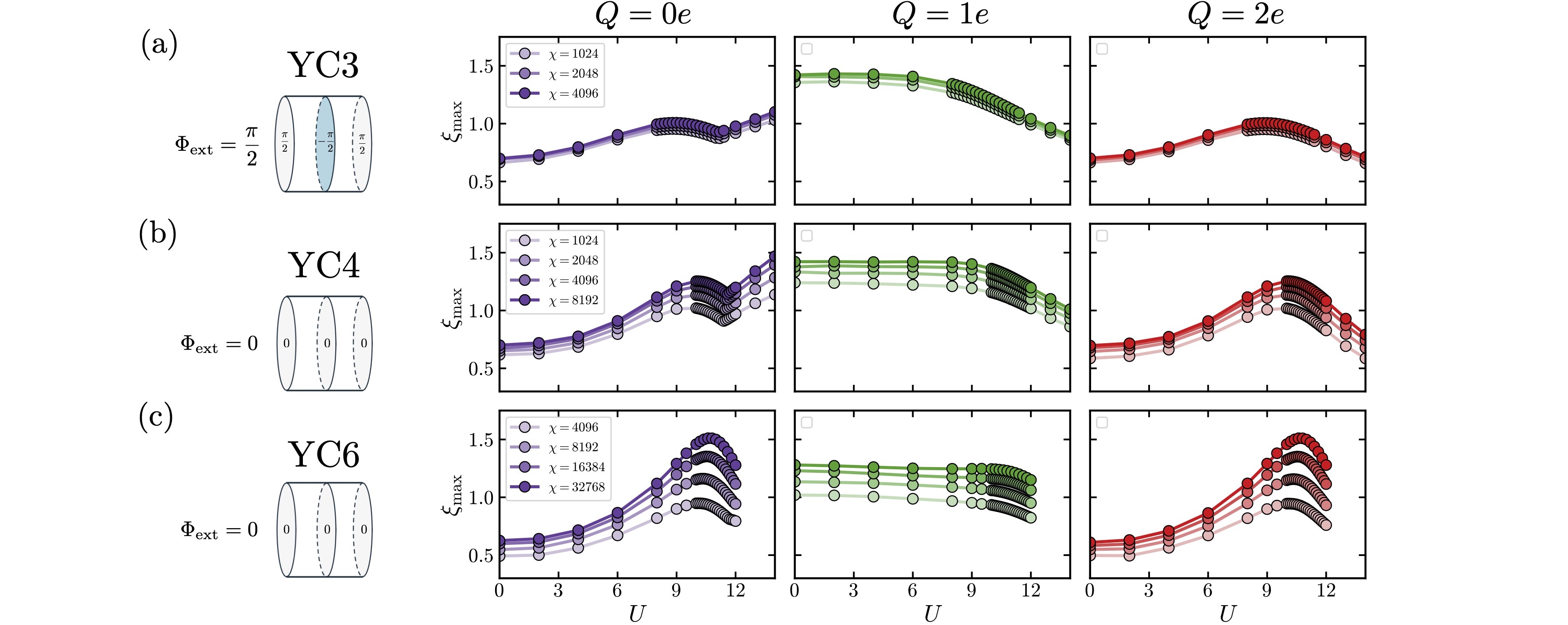
Figure A2: (a) Maximum correlation length of the half-filled ground state transfer matrix on the infinite YC3 cylinder vs. Hubbard $U$ in the charge sectors $Q\in\{0e,1e,2e\}$. External flux is threaded so that the cylinder rings are penetrated by the alternating pattern of $\pi/2,-\pi/2,\dots$ flux. Bond dimension, increasing with shade light-to-dark, indicated in legend. (b) Same for the YC4 infinite cylinder with zero flux through each ring. (c) Same for YC6 cylinder with zero flux through each ring.

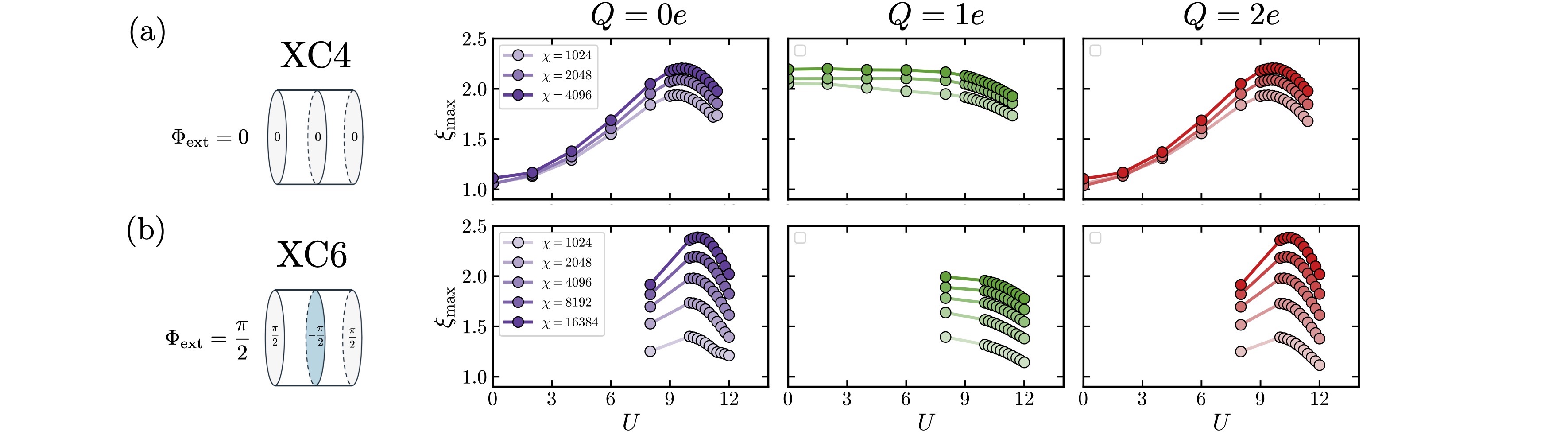
Figure A3: (a) Maximum correlation length of the half-filled ground state transfer matrix on the infinite XC4 cylinder vs. Hubbard $U$ in the charge sectors $Q\in\{0e,1e,2e\}$. Bond dimension, increasing light-to-dark with shade, indicated in legend. (b) Same for XC6 cylinder with external flux threaded so that the cylinder rings have alternating $\pi/2,-\pi/2,\dots$ flux.

Appendix E Spin and Pseudospin SU(2) Formalism

SI Relation between spin and pseudospin generators

Here we present an alternative description, complementing the Majorana representation discussed in Sec. II of the main text, of how the presence of particle-hole symmetry and Hubbard interactions gives rise to the pseudospin $\mathrm{SU}(2)_{c}$ symmetry [129]. We begin with the familiar spin rotation generators:

$$S^{+}=\sum_{\bm{r}}c_{\bm{r}\uparrow}^{\dagger}c_{\bm{r}\downarrow},\qquad S^{-}=\sum_{\bm{r}}c_{\bm{r}\downarrow}^{\dagger}c_{\bm{r}\uparrow},\qquad S^{z}=\frac{1}{2}\sum_{\bm{r}}(n_{\bm{r}\uparrow}-n_{\bm{r}\downarrow}).$$ (48)

Given a particle hole symmetry $\mathcal{P}c_{\bm{r}\sigma}\mathcal{P}^{-1}=e^{i\alpha_{\bm{r}}}c_{\bm{r}\sigma}^{\dagger}$, which commutes with the Hamiltonian, let us define the following half-particle-hole transformation:

$$\bar{\mathcal{P}}c_{\bm{r}\uparrow}\bar{\mathcal{P}}^{-1}=e^{i\alpha_{\bm{r}}}c^{\dagger}_{\bm{r}\uparrow},\qquad\bar{\mathcal{P}}c_{\bm{r}\downarrow}\bar{\mathcal{P}}^{-1}=c_{\bm{r}\downarrow}.$$ (49)

Though the half-PH leaves the spin-rotation-symmetric hopping Hamiltonian invariant, it is not a symmetry of the interaction since it flips the sign of the Hubbard $U$:

$$\bar{\mathcal{P}}\left(U\sum_{\bm{r}}(n_{\bm{r}\uparrow}-1/2)(n_{\bm{r}\downarrow}-1/2)\right)\bar{\mathcal{P}}^{-1}=U\sum_{\bm{r}}(1-n_{\bm{r}\uparrow}-1/2)(n_{\bm{r}\downarrow}-1/2)=-U\sum_{\bm{r}}(n_{\bm{r}\uparrow}-1/2)(n_{\bm{r}\downarrow}-1/2).$$ (50)

Since $H_{-U}$ also commutes with the spin generators, then $\bar{\mathcal{P}}S^{\alpha}\bar{\mathcal{P}}^{-1}$ are symmetries of $H_{+U}.$ In particular, note that

$$\eta^{+}\equiv\bar{\mathcal{P}}S^{+}\bar{\mathcal{P}}^{-1}=\sum_{\bm{r}}e^{-i\alpha_{\bm{r}}}c_{\bm{r}\uparrow}c_{\bm{r}\downarrow},$$ (51)

while

$$\eta^{z}\equiv\bar{\mathcal{P}}S^{z}\bar{\mathcal{P}}^{-1}=\frac{1}{2}\sum_{\bm{r}}(1-n_{\bm{r}\uparrow}-n_{\bm{r}\downarrow})$$ (52)

is related to the total charge density. While the resulting symmetries seem unnatural (in that $\eta^{z}$ includes a minus sign relative to the charge density and $\eta^{+}$ lowers the total charge by $2e$), we will show later that this convention is the most natural for implementing spin and pseudospin rotations simultaneously as left and right actions, respectively, in a way that is consistent with $\bar{\mathcal{P}}$ relating the generators, as in Eqs. (6-8) of Ref. [50]. Also, note that one can simply take $e^{i\alpha_{\bm{r}}}=1$ when the hoppings are all imaginary, so that:

$$\mathcal{P}c_{\bm{r}\sigma}\mathcal{P}^{-1}=c_{\bm{r}\sigma}^{\dagger}.$$ (53)

SII Fermionic matrix structure in $\mathrm{SU}(2)_{s}\times\mathrm{SU}(2)_{c}$ formalism

In order to get an analytic handle on how various $0e$ and $\pm 2e$ objects transform into one another under the pseudo SU(2) symmetry, it is useful to establish several identities. In particular, here we motivate defining the $2\times 2$ fermion construction where spin (pseudospin) rotations act on the left (right). We know that the column vector of fermion annihilation operators transforms as a spin doublet: defining

$$C_{\bm{r}}=\begin{pmatrix}c_{\bm{r}\uparrow}\\ c_{\bm{r}\downarrow}\end{pmatrix},$$ (54)

then $[S_{a},c_{s}]=-\frac{(\sigma_{a})_{ss^{\prime}}}{2}c_{s^{\prime}}$, so that

$$[\bm{S},C_{\bm{r}}]=-\frac{\bm{\sigma}}{2}C_{\bm{r}},\qquad[\bm{S},C_{\bm{r}}^{\dagger}]=C_{\bm{r}}^{\dagger}\frac{\bm{\sigma}}{2}.$$ (55)

Exponentiating these relations, we get

$$e^{i\bm{\theta}\cdot\bm{S}}C_{\bm{r}}e^{-i\bm{\theta}\cdot\bm{S}}=e^{-i\bm{\theta}\cdot\bm{\sigma}/2}C_{\bm{r}}.$$ (56)

Now it’s easy to obtain the analogous relation for the pseudospin SU(2) generators via the mapping $\bm{\eta}=\bar{\mathcal{P}}\bm{S}\bar{\mathcal{P}}^{\dagger}.$ We simply conjugate both sides by $\bar{\mathcal{P}}$ and use the fact that $\bar{\mathcal{P}}C_{\bm{r}}\bar{\mathcal{P}}^{\dagger}=\begin{pmatrix}c_{\bm{r}\uparrow}^{\dagger}\\ c_{\bm{r}\downarrow}\end{pmatrix}.$ For the infinitesimal relations, we obtain $[\bm{\eta},\begin{pmatrix}c_{\bm{r}\uparrow}^{\dagger}\\ c_{\bm{r}\downarrow}\end{pmatrix}]=-\frac{\bm{\sigma}}{2}\begin{pmatrix}c_{\bm{r}\uparrow}^{\dagger}\\ c_{\bm{r}\downarrow}\end{pmatrix},$ or by taking the Hermitian conjugate,

$$\left[\bm{\eta},\begin{pmatrix}c_{\bm{r}\uparrow}&c_{\bm{r}\downarrow}^{\dagger}\end{pmatrix}\right]=\begin{pmatrix}c_{\bm{r}\uparrow}&c_{\bm{r}\downarrow}^{\dagger}\end{pmatrix}\frac{\bm{\tau}}{2}.$$ (57)

(we have relabeled the Pauli matrices as $\bm{\tau}$ when they act to the right as pseudospin rotations). Exponentiating gives

$$e^{i\bm{\theta}\cdot\bm{\eta}}\begin{pmatrix}c_{\bm{r}\uparrow}&c_{\bm{r}\downarrow}^{\dagger}\end{pmatrix}e^{-i\bm{\theta}\cdot\bm{\eta}}=\begin{pmatrix}c_{\bm{r}\uparrow}&c_{\bm{r}\downarrow}^{\dagger}\end{pmatrix}e^{i\bm{\theta}\cdot\bm{\tau}/2}.$$ (58)

Thus $\begin{pmatrix}c_{\bm{r}\uparrow}&c_{\bm{r}\downarrow}^{\dagger}\end{pmatrix}$ should be a row of the $2\times 2$ fermion matrix. It turns out that completing this matrix with $-c_{\bm{r}\uparrow}^{\dagger}$ as the bottom right element makes both columns (rows) transform as spin (charge) doublets. Namely,

$$\Psi_{\bm{r}}=\begin{pmatrix}c_{\bm{r}\uparrow}&c_{\bm{r}\downarrow}^{\dagger}\\ c_{\bm{r}\downarrow}&-c_{\bm{r}\uparrow}^{\dagger}\end{pmatrix}=\begin{pmatrix}C_{\bm{r}}&i\sigma_{y}C_{\bm{r}}^{*}\end{pmatrix}$$ (59)

satisfies

$$e^{i\bm{\theta}\cdot\bm{S}}\Psi_{\bm{r}}e^{-i\bm{\theta}\cdot\bm{S}}=e^{-i\bm{\theta}\cdot\bm{\sigma}/2}\Psi_{\bm{r}}$$ (60)

and, on account of the relation $\bar{\mathcal{P}}C_{\bm{r}}\bar{\mathcal{P}}^{\dagger}=C_{\bm{r}}^{\dagger},$ also satisfies

$$e^{i\bm{\theta}\cdot\bm{\eta}}\Psi_{\bm{r}}e^{-i\bm{\theta}\cdot\bm{\eta}}=\Psi_{\bm{r}}e^{i\bm{\theta}\cdot\bm{\tau}/2}.$$ (61)

We also remark that the spin and charge generators can be neatly written in terms of this fermionic matrix. First:

$$\bm{S}_{\bm{r}}=\frac{1}{4}\text{tr}\left(\Psi_{\bm{r}}^{\dagger}\bm{\sigma}\Psi_{\bm{r}}\right),$$ (62)

which naturally transforms as a vector under spin rotations. Using the half-PH change of basis, we directly obtain

$$\bm{\eta}_{\bm{r}}=\bar{\mathcal{P}}\bm{S}\bar{\mathcal{P}}^{\dagger}=\frac{1}{4}\text{tr}\left(\Psi_{\bm{r}}\bm{\tau}\Psi_{\bm{r}}^{\dagger}\right),$$ (63)

where we have once again trivially rewritten the charge Pauli matrices as $\bm{\tau}.$

Finally, we note a useful implementation of the Hermitian conjugate:

$$\Psi_{\bm{r}}^{\dagger}=\begin{pmatrix}c_{\bm{r}\uparrow}^{\dagger}&c_{\bm{r}\downarrow}^{\dagger}\\ c_{\bm{r}\downarrow}&-c_{\bm{r}\uparrow}\end{pmatrix}=-\sigma_{y}\begin{pmatrix}c_{\bm{r}\uparrow}&c_{\bm{r}\downarrow}\\ c_{\bm{r}\downarrow}^{\dagger}&-c_{\bm{r}\uparrow}^{\dagger}\end{pmatrix}\sigma_{y}=-\tau_{y}\Psi_{\bm{r}}^{\mathsf{T}}\sigma_{y}.$$ (64)

This can be useful when contracting multiple $\Psi_{\bm{r}}$ under a trace, but one has to be careful about extra minus signs from fermion anti-commutation.

SIII Hofstadter-Hubbard Hamiltonian

Suppose we are given a hopping model $h=-\sum_{\bm{r},\bm{r}^{\prime}}t_{\bm{r}\bm{r}^{\prime}}c^{\dagger}_{\bm{r}}c_{\bm{r}^{\prime}}$ where $\bm{r},\bm{r}^{\prime}$ each run over all the sites in the triangular lattice. As usual, Hermiticity requires that

$$t_{\bm{r}\bm{r}^{\prime}}=t_{\bm{r}^{\prime}\bm{r}}^{*}.$$ (65)

If we further suppose that the hoppings are all imaginary, then

$$t_{\bm{r}\bm{r}^{\prime}}=-t_{\bm{r}^{\prime}\bm{r}}.$$ (66)

In particular, this means the Hamiltonian has the particle-hole symmetry $\mathcal{P}c_{\bm{r}}\mathcal{P}^{-1}=c_{\bm{r}}^{\dagger}$, like our $\Phi_{\text{$\triangle$}}=\pi/2$ Hofstadter model on the triangular lattice. In the general case, we claim that the hopping Hamiltonian can be written as

$$h=-\sum_{\bm{r}\leftarrow\bm{r}^{\prime}}t_{\bm{r}\bm{r}^{\prime}}\text{tr}\left(\Psi_{\bm{r}}^{\dagger}\Psi_{\bm{r}^{\prime}}\right),$$ (67)

where the sum is over oriented pairs of sites, which we denote by $\bm{r}\leftarrow\bm{r}^{\prime}$, whose orientation we fix so that $t_{\bm{r}\bm{r}^{\prime}}=+it$ (with $t>0$) which gives

$$h=-it\sum_{\bm{r}\leftarrow\bm{r}^{\prime}}\text{tr}\left(\Psi_{\bm{r}}^{\dagger}\Psi_{\bm{r}^{\prime}}\right).$$ (68)

The Hamiltonian is already Hermitian in this form. To see this, we explicitly compute its Hermitian conjugate:

$$h^{\dagger} =-\sum_{\bm{r}\leftarrow\bm{r}^{\prime}}t_{\bm{r}\bm{r}^{\prime}}^{*}\text{tr}\left(\Psi_{\bm{r}^{\prime}}^{\dagger}\Psi_{\bm{r}}\right)=+\sum_{\bm{r}\leftarrow\bm{r}^{\prime}}t_{\bm{r}\bm{r}^{\prime}}\text{tr}\left(\left(-\tau_{y}\Psi_{\bm{r}^{\prime}}^{\mathsf{T}}\sigma_{y}\right)\left(-\sigma_{y}(\Psi_{\bm{r}}^{\dagger})^{\mathsf{T}}\tau_{y}\right)\right),$$ (69)

where we used Eq. 64. After the Pauli matrices and minus signs cancel, we anti-commute the two operators (they live on different sites) and confirm that

$$h^{\dagger}=-\sum_{\bm{r}\leftarrow\bm{r}^{\prime}}t_{\bm{r}\bm{r}^{\prime}}\text{tr}\left((\Psi_{\bm{r}}^{\dagger})^{\mathsf{T}}\Psi_{\bm{r}^{\prime}}^{\mathsf{T}}\right)=-\sum_{\bm{r}\leftarrow\bm{r}^{\prime}}t_{\bm{r}\bm{r}^{\prime}}\text{tr}\left(\Psi_{\bm{r}}^{\dagger}\Psi_{\bm{r}^{\prime}}\right)=h.$$ (70)

We note that it is manifestly spin- and pseudospin-rotation-invariant due to the trace. To verify that $h$ is indeed the familiar hopping Hamiltonian, we explicitly expand out the expression:

$$h =-\sum_{\bm{r}\leftarrow\bm{r}^{\prime}}t_{\bm{r}\bm{r}^{\prime}}\text{tr}\left(\begin{pmatrix}c_{\bm{r}\uparrow}^{\dagger}&c_{\bm{r}\downarrow}^{\dagger}\\ c_{\bm{r}\downarrow}&-c_{\bm{r}\uparrow}\end{pmatrix}\begin{pmatrix}c_{\bm{r}^{\prime}\uparrow}&c_{\bm{r}^{\prime}\downarrow}^{\dagger}\\ c_{\bm{r}^{\prime}\downarrow}&-c_{\bm{r}^{\prime}\uparrow}^{\dagger}\end{pmatrix}\right)$$ (71)

$$=-\sum_{\bm{r}\leftarrow\bm{r}^{\prime}}(t_{\bm{r}\bm{r}^{\prime}}c_{\bm{r}s}^{\dagger}c_{\bm{r}^{\prime}s}+t_{\bm{r}\bm{r}^{\prime}}c_{\bm{r}s}c_{\bm{r}^{\prime}s}^{\dagger})$$ (72)

$$=-\sum_{\bm{r}\leftarrow\bm{r}^{\prime}}(t_{\bm{r}\bm{r}^{\prime}}c_{\bm{r}s}^{\dagger}c_{\bm{r}^{\prime}s}+t_{\bm{r}\bm{r}^{\prime}}^{*}c_{\bm{r}^{\prime}s}^{\dagger}c_{\bm{r}s})$$ (73)

$$=-\sum_{\bm{r}\leftarrow\bm{r}^{\prime}}(t_{\bm{r}\bm{r}^{\prime}}c_{\bm{r}s}^{\dagger}c_{\bm{r}^{\prime}s}+h.c.),$$ (74)

where we again used the fact that $\bm{r}\neq\bm{r}^{\prime},$ and for the last equality we crucially used the imaginary condition, Eq. (66).

As for the Hubbard interaction, we reference Ref. [50]:

$$H_{U}=\frac{2U}{3}\sum_{\bm{r}}\left(\eta_{\bm{r}}^{2}-\frac{3}{8}\right),$$ (75)

which is clearly also invariant under both spin (because $[\bm{\eta},\bm{S}]=0)$ and pseudospin rotations.

Appendix F SU(2) Slave-Rotor Theory of IQH-CSL transition

The presence of both $\mathrm{SU}(2)_{s}$ and pseudospin symmetries $\mathrm{SU}(2)_{c}$ enables an SU(2) slave-rotor analysis of the IQH, CSL, and their critical point. The construction was introduced by Hermele in Ref. [50] in the context of Hubbard models on bipartite lattices, but applies in the present context with almost no modification. The main difference is that since the triangular lattice has no natural sublattice, we instead work in the Imaginary C6 gauge (with all imaginary hoppings), where the particle-hole acts as in Eq. (53) above. This means we don’t need to keep track of a sublattice-dependent sign, i.e., Hermele’s $\epsilon_{A/B}=\pm 1$.

SI Physical Hilbert space from parton constraint

We begin by decomposing the electron operators into spinons and rotors:

$$\Psi_{\bm{r}}=F_{\bm{r}}Z_{\bm{r}},\qquad F_{\bm{r}}=\begin{pmatrix}f_{\bm{r}\uparrow}&f_{\bm{r}\downarrow}^{\dagger}\\ f_{\bm{r}\downarrow}&-f_{\bm{r}\uparrow}^{\dagger}\end{pmatrix},\qquad Z_{\bm{r}}=\begin{pmatrix}z_{\bm{r}1}&z_{\bm{r}2}\\ -z_{\bm{r}2}^{\dagger}&z_{\bm{r}1}^{\dagger}\end{pmatrix}.$$ (76)

The spinon operators are arranged like the electron operators, with spin acting by SU(2) rotations from the left, whereas gauge rotations act from the right. The rotor $Z_{\bm{r}}$ is an SU(2) matrix of operators (meaning $z_{\bm{r}1}^{\dagger}z_{\bm{r}1}+z_{\bm{r}2}^{\dagger}z_{\bm{r}2}=1$), with gauge rotations acting from the left and pseudospin rotations acting from the right. The enlarged slave-rotor Hilbert space at each site is a product of that of the spin-1/2 spinons and that of the SU(2) rotor. Since the slave-rotor Hilbert space is much larger than the physical one, we have to specify which of its states are physical. Following Ref. [50], one projects to the subspace of gauge singlets, $\bm{J}_{G}(\bm{r})=0$, where:

$$\bm{J}_{G}(\bm{r})=\frac{1}{4}\text{tr}\left(F_{\bm{r}}\bm{\mu}F_{\bm{r}}^{\dagger}\right)+\frac{1}{4}\text{tr}\left(Z_{\bm{r}}^{\dagger}\bm{\mu}Z_{\bm{r}}\right),$$ (77)

so that

$$e^{i\bm{\alpha}\cdot\bm{J}_{G}(\bm{r})}Z_{\bm{r}}e^{-i\bm{\alpha}\cdot\bm{J}_{G}(\bm{r})} =e^{-i\bm{\alpha}\cdot\bm{\mu}/2}Z_{\bm{r}},$$ (78)

$$e^{i\bm{\alpha}\cdot\bm{J}_{G}(\bm{r})}F_{\bm{r}}e^{-i\bm{\alpha}\cdot\bm{J}_{G}(\bm{r})} =F_{\bm{r}}e^{i\bm{\alpha}\cdot\bm{\mu}/2}.$$ (79)

We have denoted the Pauli matrices acting in the gauge space by $\bm{\mu}$, reserving $\bm{\sigma}$ for the spin space and $\bm{\tau}$ for the pseudospin space, as in Sec. SII above.

Note that the $F$-$Z$ Hamiltonian—obtained by writing the Hamiltonian in terms of partons—is a gauge-singlet operator. It therefore acts within the $\bm{J}_{G}(\bm{r})=0$ subspace and has the same matrix elements as the electronic Hamiltonian. To construct this subspace, which is four-dimensional at each site, we start with the slave-particle vacuum:

$$|0\rangle_{\text{sp}}=|0\rangle_{f}\otimes|0\rangle_{\text{rot}},$$ (80)

where $|0\rangle_{f}$ is the spinon vacuum and $|0\rangle_{\text{rot}}=|\ell_{C}=0,\ell_{G}=0,m_{C}=0,m_{G}=0\rangle$ is the unique rotationally-invariant state in the rotor Hilbert space ($C$ stands for “charge” pseudospin and $G$ stands for gauge); recall from Ref. [50] that only $\ell_{G}=\ell_{C}$ states are allowed to begin with. In particular, $\bm{J}_{G}(\bm{r})|0\rangle_{\text{rot}}=0$ by definition. Then it can be shown that while $|0\rangle_{\mathrm{sp}}$ is not a physical state, $f_{\bm{r}\uparrow}^{\dagger}|0\rangle_{\text{sp}}$ is physical, i.e., it is a gauge-singlet. Similarly, $f_{\bm{r}\downarrow}^{\dagger}|0\rangle_{\text{sp}}$ is a physical state. We can then construct the fully-filled and empty states by applying electronic operators:

$$c_{\bm{r}\uparrow}^{\dagger}f_{\bm{r}\downarrow}^{\dagger}|0\rangle_{\text{sp}}=(f_{\bm{r}\uparrow}^{\dagger}z_{\bm{r}1}^{\dagger}-f_{\bm{r}\downarrow}z_{\bm{r}2})f_{\bm{r}\downarrow}^{\dagger}|0\rangle_{\text{sp}}=(z_{\bm{r}1}^{\dagger}f_{\bm{r}\uparrow}^{\dagger}f_{\bm{r}\downarrow}^{\dagger}-z_{\bm{r}2})|0\rangle_{\text{sp}},$$ (81)

and

$$c_{\bm{r}\uparrow}f_{\bm{r}\uparrow}^{\dagger}|0\rangle_{\text{sp}}=(f_{\bm{r}\uparrow}z_{\bm{r}1}-f_{\bm{r}\downarrow}^{\dagger}z_{\bm{r}2}^{\dagger})f_{\bm{r}\uparrow}^{\dagger}|0\rangle_{\text{sp}}=(z_{\bm{r}1}+z_{\bm{r}2}^{\dagger}f_{\bm{r}\uparrow}^{\dagger}f_{\bm{r}\downarrow}^{\dagger})|0\rangle_{\text{sp}}.$$ (82)

Since the electron operators are invariant under gauge transformations, then both of these states are gauge singlets. We have therefore generated the full four-dimensional physical on-site Hilbert space.

SII Functional integral representation

Following the path integral construction outlined in Ref. [50], the electronic Hofstadter-Hubbard Hamiltonian can now be written in the slave-rotor representation:

$$H_{\text{HH}}=-\sum_{\bm{r},\bm{r}^{\prime}}\text{tr}\left[(F_{\bm{r}}Z_{\bm{r}})^{\dagger}(F_{\bm{r}^{\prime}}Z_{\bm{r}^{\prime}})\right]+\frac{2U}{3}\sum_{\bm{r}}\eta_{\bm{r}}^{2},$$ (83)

which must be accompanied by the aforementioned “gauge-singlet” constraint

$$\bm{J}_{\bm{G}}(\bm{r})=0.$$ (84)

Working at zero temperature, we introduce imaginary time $\tau\in(-\infty,+\infty)$ and write the functional integral:

$$\mathcal{Z}=\int\mathcal{D}Z\mathcal{D}F\mathcal{D}\bm{a}_{\tau}e^{-S},\qquad S=S_{Z}+S_{F}+S_{t},$$ (85)

where

$$S_{Z} =\frac{3}{4U}\sum_{\bm{r}}\int d\tau\ \text{tr}\left[Z^{\dagger}_{\bm{r}}\left(\overleftarrow{\partial}_{\tau}-\frac{i\bm{a}_{\tau}\cdot\bm{\mu}}{2}\right)\left({\partial}_{\tau}+\frac{i\bm{a}_{\tau}\cdot\bm{\mu}}{2}\right)Z_{\bm{r}}\right],$$ (86)

$$S_{F} =\frac{1}{2}\sum_{\bm{r}}\int d\tau\ \text{tr}\left[F_{\bm{r}}\left({\partial}_{\tau}+\frac{i\bm{a}_{\tau}\cdot\bm{\mu}}{2}\right)F_{\bm{r}}^{\dagger}\right],$$ (87)

$$S_{t} =-it\int d\tau\sum_{\bm{r}\leftarrow\bm{r}^{\prime}}\text{tr}\left[(F_{\bm{r}}Z_{\bm{r}})^{\dagger}(F_{\bm{r}^{\prime}}Z_{\bm{r}^{\prime}})\right].$$ (88)

Here and below, $\overleftarrow{\partial}$ denotes differentiation acting to the left, and the gauge field $\bm{a}_{\tau}$ has been introduced to enforce the on-site gauge constraint (Eq. 84).

So far everything is exact and therefore intractable, so we pass to a mean-field approximation. The first step is to replace the constraint $Z_{\bm{r}}(\tau)\in\mathrm{SU(2)}$ with an equivalent Lagrange multiplier term:

$$S_{\lambda}=i\int d\tau\sum_{\bm{r}}\lambda_{\bm{r}}(\tau)\left[\frac{1}{2}\text{tr}(Z^{\dagger}_{\bm{r}}Z_{\bm{r}})-1\right].$$ (89)

The next step is to decouple the hopping term into separate spinon and rotor terms. This is done by introducing a complex Hubbard–Stratonovich field via the identity [130, 50]:

$$e^{\epsilon\alpha_{\bm{r}\bm{r}^{\prime}}\beta_{\bm{r}\bm{r}^{\prime}}}=\frac{\epsilon}{\pi}\int d\eta_{\bm{r}\bm{r}^{\prime}}d\eta_{\bm{r}\bm{r}^{\prime}}^{*}\ e^{-\epsilon(|\eta_{\bm{r}\bm{r}^{\prime}}|^{2}-\eta_{\bm{r}\bm{r}^{\prime}}\alpha_{\bm{r}\bm{r}^{\prime}}-\eta_{\bm{r}\bm{r}^{\prime}}^{*}\beta_{\bm{r}\bm{r}^{\prime}})}.$$

Since we have fixed the bond orientation for the hopping in Eq. (88) above, and since $S_{t}=t\int d\tau\sum_{\bm{r}\leftarrow\bm{r}^{\prime}}(-Z_{\bm{r}^{\prime}}Z_{\bm{r}}^{\dagger})_{ab}(iF_{\bm{r}}^{\dagger}F_{\bm{r}^{\prime}})_{ba},$ then we may assign $\epsilon=t\Delta\tau>0$ and for each $a,b$ assign $\alpha_{\bm{r}\bm{r}^{\prime}}^{ab}=-(Z_{\bm{r}^{\prime}}Z_{\bm{r}}^{\dagger})_{ab}$ and $\beta_{\bm{r}\bm{r}^{\prime}}=(iF_{\bm{r}}^{\dagger}F_{\bm{r}^{\prime}})_{ba},$ which yields:

$$S_{\eta} =t\int d\tau\sum_{\bm{r}\leftarrow\bm{r}^{\prime}}\text{tr}\left[(\eta_{\bm{r}\bm{r}^{\prime}})^{\dagger}\eta_{\bm{r}\bm{r}^{\prime}}\right],$$

$$S_{tZ} =-t\int d\tau\sum_{\bm{r}\leftarrow\bm{r}^{\prime}}\text{tr}\left[Z_{\bm{r}}^{\dagger}\eta_{\bm{r}\bm{r}^{\prime}}Z_{\bm{r}^{\prime}}\right],$$

$$S_{tF} =it\int d\tau\sum_{\bm{r}\leftarrow\bm{r}^{\prime}}\text{tr}\left[F_{\bm{r}^{\prime}}(\eta_{\bm{r}\bm{r}^{\prime}})^{\dagger}F_{\bm{r}}^{\dagger}\right].$$

One obtains a real free energy at the saddle point provided that $\eta_{\bm{r}\bm{r}^{\prime}}=\chi_{\bm{r}\bm{r}^{\prime}}U_{\bm{r}\bm{r}^{\prime}}$ is a real number times an SU(2) matrix, as can be shown using the identity Eq. (64) above. In particular, two of the saddle point equations read $(\eta_{\bm{r}\bm{r}^{\prime}})^{\dagger}=\langle Z_{\bm{r}^{\prime}}Z_{\bm{r}}^{\dagger}\rangle$ and $\eta_{\bm{r}\bm{r}^{\prime}}=(t_{\bm{r}\bm{r}^{\prime}}/|t_{\bm{r}\bm{r}^{\prime}}|)\langle F_{\bm{r}}^{\dagger}F_{\bm{r}^{\prime}}\rangle=i\langle F_{\bm{r}}^{\dagger}F_{\bm{r}^{\prime}}\rangle.$ We take an ansatz where $\langle F_{\bm{r}}^{\dagger}F_{\bm{r}^{\prime}}\rangle$ is proportional to $\langle\Psi_{\bm{r}}^{\dagger}\Psi_{\bm{r}^{\prime}}\rangle$ in the $U=0$ IQH phase, producing a solution $\eta_{\bm{r}\bm{r}^{\prime}}^{*}$ (at $\bm{a}_{\tau}=0).$

Fluctuations about this solution are parameterized by an SU(2) gauge-field on the links $\bm{r}\leftarrow\bm{r}^{\prime}$ and by a fluctuating $\bm{a}_{\tau}$ component. Integrating out the spinons while retaining these gauge field degrees of freedom, then in the continuum limit we obtain at leading order in the gauge fields [131]:

$$S_{\text{CS}}=\frac{i}{4\pi}\int d^{3}x\ \epsilon^{\mu\nu\rho}\text{tr}\left(a_{\mu}\partial_{\nu}a_{\rho}+\frac{2}{3}a_{\mu}a_{\nu}a_{\rho}\right),$$

which is an SU(2) Chern-Simons term at level 1 [132].

SIII Low-energy $\mathrm{SU(2)}_{1}$ Higgs-Chern-Simons theory

To describe the IQH-CSL transition, we pass to a continuum description of the rotor bosons. We begin with the mean-field action

$$S_{\text{MF}}^{Z}=-\sum_{\tau,\bm{r}}\left[\text{tr}Z_{x+\epsilon z}^{\dagger}Z_{x}+h.c.\right]-\sum_{\tau}\sum_{\langle\bm{r},\bm{r}^{\prime}\rangle}\left[\text{tr}Z_{\bm{r},\tau}^{\dagger}Z_{\bm{r}^{\prime},\tau}+h.c.\right]+\frac{r+r_{c0}}{2}\sum_{\tau,\bm{r}}\left[\text{tr}Z_{x}^{\dagger}Z_{x}\right],$$ (90)

where $r_{c0}$ is chosen so that the lowest boson mode goes gapless as $r\to 0^{+}.$ Following Ref. [50], we take a spacetime lattice of triangular lattice sites separated by $\epsilon$ increments in imaginary time. For $r>0,$ diagonalizing the above spacetime-translation-invariant Hamiltonian gives a unique low-energy mode at $\bm{q}=0,$ consistent with the rotors experiencing no net flux. We write $\Theta(x)\sim Z_{\bm{r},t}$ with $x$ now a continuous spacetime coordinate, which yields:

$$\mathcal{L}_{\text{0}}^{\Theta}=\frac{1}{2}\text{tr}(\Theta^{\dagger}\overleftarrow{\partial}_{\nu}\partial_{\nu}\Theta)+\frac{r}{2}\text{tr}(\Theta^{\dagger}\Theta),$$ (91)

where $\overleftarrow{\partial}$ denotes differentiation to the left. Note that demanding invariance under global SU(2) gauge transformations and pseudospin rotations precludes a linear time-derivative term $\sim\text{tr}(\Theta^{\dagger}\partial_{\tau}\Theta).$ This entirely fixes the form at $\mathcal{L}_{\text{0}}^{\Theta}$ quadratic order. Now we add the gauge field fluctuations by promoting the derivative to the covariant derivative

$$\partial_{\nu}\to\partial_{\nu}+\frac{i\bm{a}_{\nu}\cdot\bm{\mu}}{2},$$ (92)

giving

$$\mathcal{L}_{\text{kin}}^{\Theta}=\frac{1}{2}\text{tr}\left[\Theta^{\dagger}\left(\overleftarrow{\partial}_{\mu}-\frac{ia_{\mu}^{j}\sigma^{i}}{2}\right)\left(\overrightarrow{\partial}_{\mu}+\frac{ia_{\mu}^{j}\sigma^{i}}{2}\right)\Theta\right],$$ (93)

where $\bm{\mu}$ is again the Pauli matrix vector in the gauge space. Reintroducing the $\mathrm{SU(2)}{}_{1}$ Chern-Simons term from integrating out the spinons, and the symmetry-allowed quartic term, the full SU(2) Higgs-Chern-Simons theory is:

$$\mathcal{L}_{\text{eff}}=\mathcal{L}_{\text{CS}}+\mathcal{L}_{\text{kin}}^{\Theta}+\frac{1}{2}\text{tr}(\Theta^{\dagger}\Theta)+\frac{\lambda}{4}\left[\text{tr}(\Theta^{\dagger}\Theta)\right]{}^{2}+\dots$$ (94)

SIV Conserved current

As spin excitations are gapped across the IQH-CSL transition, and neither the spin nor pseudospin symmetries are broken, then the closing of the charge gap is associated with gapless bosonic modes that transform as spin-singlet pseudospin-triplets. We now compute the conserved Noether current associated with the pseudospin rotation $\mathrm{SU}(2)_{c}$ symmetry. The important Lagrangian term for the current is the coupling $\mathcal{L}_{\text{kin}}^{\Theta}$ between the low-energy bosonic field $\Theta$ and the SU(2) gauge field in Eq. (93) above. Under the pseudospin SU(2) rotation

$$\Theta^{\prime}=\Theta e^{i\bm{\alpha}\cdot\bm{\tau}/2}\approx\Theta+\Theta\frac{i\bm{\alpha}\cdot\bm{\tau}}{2},$$ (95)

this term transforms to

$$(\mathcal{L}_{\text{kin}}^{\Theta})^{\prime} =\frac{1}{2}\text{tr}\left[\left(\Theta^{\dagger}-\frac{i\bm{\alpha}\cdot\bm{\tau}}{2}\Theta^{\dagger}\right)\left(\overleftarrow{\partial}_{\mu}-\frac{ia_{\mu}^{j}\sigma^{i}}{2}\right)\left(\vec{\partial}_{\mu}+\frac{ia_{\mu}^{j}\sigma^{i}}{2}\right)\left(\Theta+\Theta\frac{i\bm{\alpha}\cdot\bm{\tau}}{2}\right)\right]$$ (96)

$$=\mathcal{L}_{\text{kin}}^{\Theta}+\frac{1}{2}\text{tr}\left[\left(-\frac{i\bm{\alpha}\cdot\bm{\tau}}{2}\Theta^{\dagger}\right)\left(\overleftarrow{\partial}_{\mu}-\frac{ia_{\mu}^{j}\sigma^{i}}{2}\right)\left(\vec{\partial}_{\mu}+\frac{ia_{\mu}^{j}\sigma^{i}}{2}\right)\Theta\right]$$ (97)

$$\qquad+\frac{1}{2}\text{tr}\left[\Theta^{\dagger}\left(\overleftarrow{\partial}_{\mu}-\frac{ia_{\mu}^{j}\sigma^{i}}{2}\right)\left(\vec{\partial}_{\mu}+\frac{ia_{\mu}^{j}\sigma^{i}}{2}\right)\left(\Theta\frac{i\bm{\alpha}\cdot\bm{\tau}}{2}\right)\right].$$ (98)

When $\alpha$ is constant, then $(\mathcal{L}_{\text{kin}}^{\Theta})^{\prime}=\mathcal{L}_{\text{kin}}^{\Theta}$ to all orders. When it varies in spacetime, on the other hand

$$(\mathcal{L}_{\text{kin}}^{\Theta})^{\prime}-\mathcal{L}_{\text{kin}}^{\Theta} =\frac{1}{2}\text{tr}\left[\left(-\frac{i\bm{\alpha}\cdot\bm{\tau}}{2}\Theta^{\dagger}\right)\left(\overleftarrow{\partial}_{\mu}-\frac{ia_{\mu}^{j}\sigma^{i}}{2}\right)\left(\vec{\partial}_{\mu}+\frac{ia_{\mu}^{j}\sigma^{i}}{2}\right)\Theta\right]$$ (99)

$$\qquad+\frac{1}{2}\text{tr}\left[\Theta^{\dagger}\left(\overleftarrow{\partial}_{\mu}-\frac{ia_{\mu}^{j}\sigma^{i}}{2}\right)\left(\vec{\partial}_{\mu}+\frac{ia_{\mu}^{j}\sigma^{i}}{2}\right)\left(\Theta\frac{i\bm{\alpha}\cdot\bm{\tau}}{2}\right)\right].$$ (100)

After expansion and simplification, the two terms above reduce to:

$$\frac{1}{2}\text{tr}\left[\Theta^{\dagger}\left(\overleftarrow{\partial}_{\mu}-\frac{ia_{\mu}^{j}\sigma^{i}}{2}\right)\left(\vec{\partial}_{\mu}+\frac{ia_{\mu}^{j}\sigma^{i}}{2}\right)\left(\Theta\frac{i\bm{\alpha}\cdot\bm{\tau}}{2}\right)\right] =\frac{1}{2}\text{tr}\left[\Theta^{\dagger}\left(\overleftarrow{\partial}_{\mu}-\frac{ia_{\mu}^{j}\sigma^{i}}{2}\right)\Theta\frac{i\partial_{\mu}\bm{\alpha}\cdot\bm{\tau}}{2}\right]$$ (101)

$$\qquad+\frac{1}{2}\text{tr}\left[\Theta^{\dagger}\left(\overleftarrow{\partial}_{\mu}-\frac{ia_{\mu}^{j}\sigma^{i}}{2}\right)\left(\vec{\partial}_{\mu}+\frac{ia_{\mu}^{j}\sigma^{i}}{2}\right)\Theta\times\frac{i\bm{\alpha}\cdot\bm{\tau}}{2}\right],$$ (102)

and likewise

$$\frac{1}{2}\text{tr}\left[\left(-\frac{i\bm{\alpha}\cdot\bm{\tau}}{2}\Theta^{\dagger}\right)\left(\overleftarrow{\partial}_{\mu}-\frac{ia_{\mu}^{j}\sigma^{i}}{2}\right)\left(\vec{\partial}_{\mu}+\frac{ia_{\mu}^{j}\sigma^{i}}{2}\right)\Theta\right] =-\frac{1}{2}\text{tr}\left[\frac{i\partial_{\mu}\bm{\alpha}\cdot\bm{\tau}}{2}\Theta^{\dagger}\left(\vec{\partial}_{\mu}+\frac{ia_{\mu}^{j}\sigma^{i}}{2}\right)\Theta\right]$$ (103)

$$\qquad-\frac{1}{2}\text{tr}\left[\frac{i\bm{\alpha}\cdot\bm{\tau}}{2}\times\Theta^{\dagger}\left(\overleftarrow{\partial}_{\mu}-\frac{ia_{\mu}^{j}\sigma^{i}}{2}\right)\left(\vec{\partial}_{\mu}+\frac{ia_{\mu}^{j}\sigma^{i}}{2}\right)\Theta\right].$$ (104)

By cyclicity of the trace, what remains after cancellation is:

$$(\mathcal{L}_{\text{kin}}^{\Theta})^{\prime}-\mathcal{L}_{\text{kin}}^{\Theta}=\partial_{\mu}\alpha^{j}\cdot\frac{1}{2}\text{tr}\left[\Theta^{\dagger}\left(\overleftarrow{\partial}_{\mu}-\frac{ia_{\mu}^{j}\sigma^{i}}{2}\right)\Theta\frac{i\tau^{j}}{2}-\frac{i\tau^{j}}{2}\Theta^{\dagger}\left(\vec{\partial}_{\mu}+\frac{ia_{\mu}^{j}\sigma^{i}}{2}\right)\Theta\right],$$ (105)

so that the conserved current is

$$\bm{\mathcal{J}}_{\mu}\propto\text{tr}\left[\frac{\bm{\tau}}{2}\frac{\Theta^{\dagger}\left(\vec{\partial}_{\mu}+\frac{ia_{\mu}^{j}\sigma^{i}}{2}\right)\Theta-\Theta^{\dagger}\left(\overleftarrow{\partial}_{\mu}-\frac{ia_{\mu}^{j}\sigma^{i}}{2}\right)\Theta}{2i}\right]=\text{tr}\left[\frac{\bm{\tau}}{2}\frac{\Theta^{\dagger}\vec{D}_{\mu}\Theta-\Theta^{\dagger}\overleftarrow{D}_{\mu}\Theta}{2i}\right].$$ (106)

Because of the pseudospin Pauli vector $\bm{\tau}/2$, this bosonic object transforms as a vector under global pseudospin rotations $\Theta\to\Theta e^{i\bm{\theta}\cdot\bm{\tau}/2}.$ Indeed, its $\tau^{z}$ component is like the density of low-energy Cooper pairs, while $\tau^{\pm}$ serve as Cooper pair annihilation/creation operators. Moreover, it is gauge-invariant since $D_{\mu}\Theta$ is gauge-covariant. Finally, since it is the conserved current, then at the critical point all components will have protected scaling dimension 2. Altogether, this SU(2) formulation confirms the physical conclusions made in Ref. [65], by working here in a formalism manifestly invariant under the pseudospin symmetry.

Appendix G Electron Pairing from Small-$U$ Diagrammatic Expansion

SI Band basis in the doubly-folded Brillouin zone

Let’s work in the Imaginary C6 gauge, which has four sublattice sites $\mathcal{S}=\{A,B,C,D\},$ arranged as in Fig. A1(a). While $T_{1}$ and $T_{2}$ anti-commute in the odd-fermion-parity sector, $(T_{1})^{2}$ and $(T_{2})^{2}$ commute. Thus, given displacements $\bm{d}\in\bar{\mathcal{L}}\equiv 2\mathcal{L}$ (i.e. in the $A$ sublattice), then the operators $T_{\bm{d}}$ have unambiguous action and form a group. In fact, in the Imaginary $C_{6}$ gauge with single-site translations defined as in Eq. (5), these two-site translation operators are pure coordinate shift, as shown in Eq. (6) above. Therefore we can readily apply Bloch’s theorem with a four-site unit cell. Let $\overline{\mathrm{BZ}}$ denote the “doubly-folded” Brillouin zone corresponding to $\bar{\mathcal{L}}$. The Fourier-transformed electron operators are

$$c_{\bm{k},\gamma}^{\dagger}=\frac{1}{\sqrt{|\bar{\mathcal{L}}|}}\sum_{\bm{d}\in\bar{\mathcal{L}}}e^{i\bm{k}\cdot(\bm{d}+\bm{\gamma})}T_{\bm{d}}c_{\bm{0}+\bm{\gamma}}^{\dagger}T_{\bm{d}}^{\dagger}=\frac{1}{\sqrt{|\bar{\mathcal{L}}|}}\sum_{\bm{d}\in\bar{\mathcal{L}}}e^{i\bm{k}\cdot(\bm{d}+\bm{\gamma})}c_{\bm{d}+\bm{\gamma}}^{\dagger},$$ (107)

where we used the fact that $T_{\bm{d}}$ is pure coordinate shift for $\bm{d}\in\bar{\mathcal{L}}.$

Now let’s Fourier transform the hopping Hamiltonian, namely

$$h=-\sum_{\bm{r},\bm{r}^{\prime}}t_{\bm{r}\bm{r}^{\prime}}c_{\bm{r}}^{\dagger}c_{\bm{r}^{\prime}}=-\sum_{\gamma,\gamma^{\prime}}\sum_{\bm{d},\bm{d}^{\prime}\in\bar{\mathcal{L}}}t_{\bm{d}+\bm{\gamma},\bm{d}^{\prime}+\bm{\gamma}^{\prime}}c_{\bm{d}+\bm{\gamma}}^{\dagger}c_{\bm{d}^{\prime}+\bm{\gamma}^{\prime}},$$ (108)

where $\gamma,\gamma^{\prime}$ run over the sublattices $\mathcal{S}$ and

$$t_{\bm{d}+\bm{\gamma},\bm{d}^{\prime}+\bm{\gamma}^{\prime}}=t_{\gamma,\gamma^{\prime}}(\bm{d}-\bm{d}^{\prime})$$ (109)

is manifestly translation-invariant on the scale of $2\mathcal{L}$. Inverting the electron Fourier transform Eq. (107), we obtain

$$c_{\bm{d}+\bm{\gamma}}^{\dagger}=\sum_{\bm{k}\in\overline{\mathrm{BZ}}}e^{-i\bm{k}\cdot(\bm{d}+\bm{\gamma})}c_{\bm{k},\gamma}^{\dagger},$$ (110)

and substituting it in gives

$$h =-\frac{1}{|\bar{\mathcal{L}}|}\sum_{\gamma,\gamma^{\prime}}\sum_{\bm{d},\bm{d}^{\prime}\in\bar{\mathcal{L}}}t_{\bm{d}+\bm{\gamma},\bm{d}^{\prime}+\bm{\gamma}^{\prime}}\left(\sum_{\bm{k}\in\overline{\mathrm{BZ}}}e^{-i\bm{k}\cdot(\bm{d}+\bm{\gamma})}c_{\bm{k},\gamma}^{\dagger}\right)\left(\sum_{\bm{k}^{\prime}\in\overline{\mathrm{BZ}}}e^{i\bm{k}^{\prime}\cdot(\bm{d}^{\prime}+\bm{\gamma}^{\prime})}c_{\bm{k}^{\prime},\gamma^{\prime}}\right)$$ (111)

$$=\sum_{\bm{k},\bm{k}^{\prime}\in\overline{\mathrm{BZ}}}\sum_{\gamma,\gamma^{\prime}}\left[-e^{-i\bm{k}\cdot\bm{\delta}}\sum_{\bm{\delta}\in\bar{\mathcal{L}}}e^{-i\bm{k}\cdot\bm{\gamma}}t_{\bm{d}+\bm{\gamma},\bm{d}^{\prime}+\bm{\gamma}^{\prime}}e^{i\bm{k}^{\prime}\cdot\bm{\gamma}^{\prime}}\right]\left(\frac{1}{|\bar{\mathcal{L}}|}\sum_{\bm{d}^{\prime}\in\bar{\mathcal{L}}}e^{i(\bm{k}^{\prime}-\bm{k})\cdot\bm{d}^{\prime}}\right)c_{\bm{k},\gamma}^{\dagger}c_{\bm{k}^{\prime},\gamma^{\prime}}$$ (112)

$$=\sum_{\bm{k}\in\overline{\mathrm{BZ}}}\sum_{\gamma,\gamma^{\prime}}c_{\bm{k},\gamma}^{\dagger}h_{\gamma,\gamma^{\prime}}(\bm{k})c_{\bm{k},\gamma^{\prime}},$$ (113)

where

$$h_{\gamma,\gamma^{\prime}}(\bm{k})=e^{-i\bm{k}\cdot\bm{\delta}}\left(-\sum_{\bm{\delta}\in\bar{\mathcal{L}}}e^{-i\bm{k}\cdot\bm{\gamma}}t_{\bm{d}+\bm{\gamma},\bm{d}^{\prime}+\bm{\gamma}^{\prime}}\right)e^{i\bm{k}^{\prime}\cdot\bm{\gamma}^{\prime}}.$$ (114)

Using $t_{\gamma^{\prime},\gamma}(-\bm{\delta})^{*}=t_{\gamma,\gamma^{\prime}}(\bm{\delta}),$ one can show that $h_{\gamma,\gamma^{\prime}}(\bm{k})$ is a Hermitian matrix in the sublattice. We plot the higher of the two resulting bands in Fig. 1(c). Note that the lower and upper bands are each two-fold degenerate, a consequence of our having folded the lattice-scale Brillouin zone not once but twice (in order to accommodate the $2\times 2$-site unit cell and $C_{6}$ rotations).

Let us denote the magnetic reciprocal lattice vectors of the magnetic lattice by

$$\bar{\mathcal{L}}^{-1}\in\mathrm{span}\left\{\bm{b}_{1}/2,\bm{b}_{2}/2\right\}$$ (115)

(where the “span” is over integer linear combinations), defined equivalently as those vectors for which $\bm{\delta}\in\bar{\mathcal{L}}\implies\bm{G}\cdot\bm{\delta}\in 2\pi\mathbb{Z}.$ Under shifts by such vectors, the Hamiltonian transforms as

$$h_{\gamma,\gamma^{\prime}}(\bm{k}+\bm{G})=e^{-i\bm{G}\cdot\bm{\gamma}}h_{\gamma,\gamma^{\prime}}(\bm{k})e^{i\bm{G}\cdot\bm{\gamma}^{\prime}}.$$ (116)

As $4\times 4$ matrices in the sublattice degree of freedom, $h(\bm{k}+\bm{G})$ is therefore unitarily-related to $h(\bm{k})$ and has the same spectrum. We obtain eigenstates by diagonalization:

$$h(\bm{k})u(\bm{k})=u(\bm{k})E(\bm{k}),$$ (117)

where $E(\bm{k})$ is a diagonal matrix of energies, while $u_{\gamma,n}(\bm{k})$ is a unitary matrix whose columns are labeled by band $n$ and whose rows are labeled by sublattice $\gamma.$ Correspondingly, the Bloch fermion creation operators are

$$f_{n}^{\dagger}(\bm{k})=\sum_{\gamma}c_{\bm{k},\gamma}^{\dagger}u_{\gamma,n}(\bm{k}),$$ (118)

which is easily shown to diagonalize the hopping Hamiltonian and satisfy the usual fermion anti-commutation relations.

SII Perturbative demonstration of odd-angular momentum spin-singlet pairing

We rewrite the model in momentum space

$$\begin{split}\mathcal{H}&=\sum_{12}c_{2}^{\dagger}h_{2,1}c_{1}+\frac{1}{2N}\sum_{1234}c_{4}^{\dagger}c_{3}^{\dagger}\Gamma_{43,21}c_{2}c_{1},\end{split}$$ (119)

with $N$ the number of unit cells, and $i=({k}_{i},o_{i},\sigma_{i})$ a generalized index gathering the single particle momentum ${k}_{i}$ belonging to the Brillouin zone (BZ), the sublattice index $o_{i}$, and the spin $\sigma_{i}$. Due to momentum and spin conservation, and because our model only features a Hubbard interaction, the parameters in this Hamiltonian can be simplified as

$$\begin{split}h_{2,1}&=\delta_{k_{1},k_{2}}\delta_{\sigma_{1},\sigma_{2}}h_{o_{2},o_{1}}(k_{1}),\\ \Gamma_{43,21}&=U\delta_{s_{4},s_{1},\uparrow}\delta_{s_{3},s_{2},\downarrow}\delta_{o_{4},o_{3},o_{2},o_{1}}\delta_{k_{1}+k_{2},k_{3}+k_{4}},\end{split}$$ (120)

Renormalization of the two-body scattering vertex is described, to second order in many-body perturbation theory, by the five diagrams [93]:

$$\leavevmode\hbox to34.54pt{\vbox to23.16pt{\text{[drawing]}}},\,\leavevmode\hbox to34.54pt{\vbox to24.09pt{\text{[drawing]}}},\,\leavevmode\hbox to34.54pt{\vbox to25.66pt{\text{[drawing]}}},\,\leavevmode\hbox to34.54pt{\vbox to25.66pt{\text{[drawing]}}},\,\leavevmode\hbox to34.54pt{\vbox to23.16pt{\text{[drawing]}}},\,$$ (121)

where curvy and straight lines respectively denote interaction events and single-particle propagators. The evaluation of these diagrams is detailed in App. D of Ref. [98], producing a renormalized interaction vertex $\Gamma^{\rm eff}=\Gamma+\delta\Gamma$, with

$$\delta\Gamma_{43,21}=-\frac{1}{N}\sum_{abcd}\chi_{dc,ba}^{-}\Gamma_{43,ba}\Gamma_{dc,21}+\chi_{dc,ba}^{+}[\Gamma_{4c,2a}\Gamma_{d3,b1}+\Gamma_{c3,2a}\Gamma_{d4,b1}+\Gamma_{4c,a1}\Gamma_{d3,b2}-N_{f}\Gamma_{4c,a1}\Gamma_{d3,2b}],$$ (122)

where the terms are ordered as their corresponding diagrams in Eq. (121) where $N_{f}=2$ is the number of spin species. The sum over the generalized indices $(a,b,c,d)$ runs over momenta, orbital and spin indices. The single-particle propagators are characterized by the Bloch eigenvectors $\Psi_{k_{i},n}^{o_{i}}$ with $n$ a band index, which are the same for both spin species. Finally, we have respectively denoted as $\chi^{-}$ and $\chi^{+}$ the particle-particle and particle-hole susceptibilities, whose explicit form is

$$\chi_{dc,ba}^{\epsilon=\pm}=\delta_{{k}_{a}}^{{k}_{d}}\delta_{{k}_{b}}^{{k}_{c}}\sum_{n,n^{\prime}=\pm}\Psi_{k_{d},n}^{o_{d}\,*}\Psi_{k_{c},n^{\prime}}^{o_{c}\,*}\Psi_{k_{b},n^{\prime}}^{o_{b}}\Psi_{k_{a},n}^{o_{a}}\frac{f_{\beta}(\epsilon\xi_{{k}_{a},n})-f_{\beta}(\xi_{{k}_{b},n^{\prime}})}{\xi_{{k}_{a},n}-\epsilon\xi_{{k}_{b},n^{\prime}}},$$

where $f_{\beta}(x)=1/[1+e^{\beta x}]$ is the Fermi-Dirac distribution, and $\xi_{i}=\varepsilon_{i}-\mu$ measures energies with respect to the chemical potential $\mu$.

We are interested in the correction to the Cooper interaction $\delta\Gamma_{(k^{\prime},\uparrow,o_{4})(-k^{\prime},\downarrow,o_{3}),(-k,\downarrow,o_{2})(k,\uparrow,o_{1})}$ at zero temperature when the chemical potential is in the middle of the gap. Several simplifications arise:

• First, the contributions of bubble and of the upper and lower wine glass diagrams vanish. This can be straightforwardly checked using the spin constraints on the bare vertex $\Gamma$.

• Second, we can see that $\chi^{-}$ only involves intra-band processes that are most relevant in presence of a Fermi surface, i.e., at finite doping which is not the focus of this pairing calculation. This simply comes from $f_{\beta}(\xi<0)=1$ and $f_{\beta}(\xi>0)=0$.

• This only leaves the crossed diagram.

Focusing on the Cooper channel, we evaluate this crossed diagram and project onto the given bands (in the Imaginary C6 gauge, there are two bands per valley above half-filling) to get

$$\delta\Gamma_{(k^{\prime},\uparrow,n_{4})(-k^{\prime},\downarrow,n_{3}),(-k,\downarrow,n_{2})(k,\uparrow,n_{1})}=-U^{2}\sum_{o,o^{\prime}}\left(\Psi_{k^{\prime},o}^{n_{4}}\Psi_{-k^{\prime},o^{\prime}}^{n_{3}}\right)^{*}\tilde{\chi}_{o^{\prime},o}(k^{\prime}+k)\left(\Psi_{-k,o}^{n_{2}}\Psi_{k,o^{\prime}}^{n_{1}}\right),$$ (123)

where the orbital susceptibilities are defined by

$$\tilde{\chi}_{o^{\prime},o}(q)=\frac{1}{N}\sum_{p}\chi_{(p+q,o^{\prime})(p,o),(p,o^{\prime})(p+q,o)}^{+}.$$ (124)

Note that in spite of the overall sign in front of the sum, this interaction is mostly repulsive because the susceptibilities defined above are negative in the density-density channel where $o=o^{\prime}$.

If we focus on the effective scattering coefficient between electrons occupying the lowest single-particle states of the model, then we can replace $k$ and $k^{\prime}$ by $\kappa/\kappa^{\prime}$. Then there are only three orbital susceptibilities to compute $\tilde{\chi}(0,\kappa,\kappa^{\prime})$ and four Bloch states to obtain in order to evaluate all the different Cooper scattering coefficients. This forms a matrix that we can diagonalize to identify the most attractive (if any). We have computed all of those terms, and have found a single attractive channel that we write in the basis where band 0 has $C_{3}$ eigenvalues $\omega$ at $\kappa/\kappa^{\prime}$, bands 1 and 3 have zero angular momentum at those points, and band 2 has angular momentum $\omega^{*}$. All of these single-electron angular momenta were computed using the conventions for gauge and $C_{6}$ described in App. SII above.

We focus on the conduction bands 2 and 3. The pairing channel we find is a spin-singlet and carries $C_{3}$ angular momentum (one electron of the pair in each band) in our choice of gauge and for our choice of rotation symmetry $C_{3}$. Examining at the pair closely, it is antisymmetric in the band index and in the valley index (hence fully antisymmetric under particle exchange, as required). The valley antisymmetry gives eigenvalue $-1$ under $C_{2}$, making explicit the odd site-centered angular momentum nature of the pair. Altogether, we can write the pair down as:

$$\hat{\Delta}=c_{\kappa^{\prime},\uparrow,\omega^{*}}c_{\kappa,\downarrow,1}+c_{\kappa,\uparrow,1}c_{\kappa^{\prime},\downarrow,\omega^{*}}-c_{\kappa^{\prime},\uparrow,1}c_{\kappa,\downarrow,\omega^{*}}-c_{\kappa,\uparrow,\omega^{*}}c_{\kappa^{\prime},\downarrow,1}.$$ (125)

Recall the discussion in the main text that $C_{3}\to(e^{2\pi i/3})^{N_{F}}C_{3}$ may be redefined, thus modifying the $C_{3}$ eigenvalue, while preserving the identity $(C_{3})^{3}=1$. Therefore, to prevent confusion, in the main text we have replaced the $C_{3}$ eigenvalue labels $1$ and $\omega^{*}$ to an index $n\in\{1,2\}$ which likewise labels the degenerate bands at each of $\kappa$ and $\kappa^{\prime}$.