Regulating Sommerfeld resonances for multi-state systems and higher partial waves

Abstract

Long-range attractive interactions between dark matter particles can significantly enhance their annihilation, particularly at low velocities. This “Sommerfeld enhancement” is typically computed by evaluating the deformation of the two-particle wavefunction due to the long-range potential, while ignoring the physics associated with the annihilation, and then scaling the appropriate annihilation matrix elements by factors that depend on the wavefunction in the limit where the particles approach zero relative separation. It has long been recognized that this approach is a valid approximation only in the limit where the annihilation rate is small, and breaks down in the regime where the enhanced annihilation rate approaches the unitarity bound, in which case ignoring the impact of the annihilation physics on the two-particle wavefunction cannot be justified and leads to apparent violations of unitarity. In the case where the physics relevant to annihilation occurs at a parametrically shorter distance scale (higher energy scale) compared with the long-range potential, we provide a simple prescription for correcting the Sommerfeld enhancement for the effects of the short-range physics, valid for all partial waves and for systems where multiple states are coupled by the long-range potential.

1 Introduction

Stable particles may experience long-range interactions either mediated by known Standard Model (SM) particles or by new forces. It was pointed out as early as 2002 Hisano:2002fk ; Hisano:2003ec ; Hisano:2004ds that such long-range interactions between annihilating dark matter (DM) particles could significantly enhance the annihilation rate, in analogy to the Sommerfeld enhancement of electron-positron annihilation via the Coulomb interaction Sommerfeld:1931qaf . The original application of this insight was in the context of heavy DM in multiplets of the SM $SU(2)_{L}$ gauge group, where the force carriers are the electroweak gauge bosons and multiple states participate in the long-range interaction; subsequent studies explored the implications of Sommerfeld enhancement for more general DM scenarios (e.g. ArkaniHamed:2008qn ; Iengo:2009ni ; Cassel:2009wt ; Slatyer:2009vg ).

The lowest-order prescription for calculating the Sommerfeld enhancement described in Refs. Hisano:2002fk ; Hisano:2003ec ; Hisano:2004ds gives the overall annihilation cross section in the factorized form:

$$\sigma v_{\text{rel}}=c_{i}\sum_{ab}A_{a}\Gamma_{ab}A_{b}^{*},$$ (1)

where $v_{\text{rel}}$ is the relative velocity between the two particles, $c_{i}$ is a symmetry coefficient dependent only on the initial state, $A$ is a vector obtained by solving the Schrödinger equation for the two-particle wavefunction in the presence of a long-range potential, and the matrix $\Gamma$ is built from the matrix elements for annihilation involving all the states coupled by the long-range potential. That long-range potential is characterized by a matrix, and includes diagonal terms corresponding to the mass splittings between the states coupled by the potential.

As already noted in Ref. Hisano:2004ds , this factorization between the long-range potential effects and the annihilation matrix is only accurate to lowest order in $\Gamma$. More generally, the possibility for the particles to annihilate should be taken into account when working out the deformation of the wavefunction; ignoring this effect can lead to apparent violations of unitarity. Specifically, this effect becomes apparent (even for weakly-coupled interactions) when there is a near-zero-energy bound state in the spectrum, leading to a resonant enhancement to the annihilation cross section. The standard approach implies an enhanced $s$-wave cross section scaling as $\sigma v_{\text{rel}}\propto v_{\text{rel}}^{-2}$ at the center of the resonance (e.g. Cassel:2009wt ), which at sufficiently low velocities contradicts the partial-wave unitarity bound $\sigma\leq 2\pi/(\mu v_{\text{rel}})^{2}$ (for inelastic scattering of indistinguishable particles, and where $\mu$ is the reduced mass of the system).

Ref. Blum:2016nrz demonstrated how to capture this effect and restore manifest unitarity for a single-state system with only $s$-wave annihilation, by modeling the effect of annihilation (and possibly other short-range physics) as a $\delta$-function potential with a complex coefficient, and solving the Schrödinger equation to obtain the wavefunction in the presence of this added term. Refs. Braaten:2017gpq ; Braaten:2017kci ; Braaten:2017dwq developed a “zero range effective field theory” (ZREFT), allowing analytic study of Sommerfeld enhancement in the neighborhood of $s$-wave resonances, for DM that is a $SU(2)_{L}$ fermion triplet; the ZREFT parameterizes the behavior near the resonance in terms of a scattering length, and accounts for the annihilation effects naturally by allowing this scattering length to be complex. The ZREFT was restricted to $s$-wave resonances, but demonstrated the generalization of the unitarization prescription to a multi-state system. Ref. Chu:2019awd suggested a general parameterization for DM self-interaction cross sections in terms of the scattering length and effective range, and demonstrated how this prescription could be applied to the case of $s$-wave annihilation. Ref. Kamada:2023iol showed the correlation between the resonant self-scattering cross section and the Sommerfeld factor for the annihilation by using Watson’s theorem.

The methodology of Ref. Blum:2016nrz did not generalize straightforwardly to higher partial waves, due to the lack of overlap between the higher-$\ell$ wavefunctions and a delta-function potential. In this work, we propose a new prescription for computing the corrected Sommerfeld enhancement, with conceptual similarities to the work of Refs. Agrawal:2020lea ; Parikh:2020ggm . The resulting expression is manifestly unitarity-preserving, requires no additional calculations beyond solving the Schrödinger equation for the long-range potential and knowledge of any relevant short-distance interactions, and can be applied to all partial waves and to multi-state systems.

The central idea is that if there is a separation of scales between annihilation and the interactions mediating the long-range potential, then we can treat the annihilation (and possibly other short-distance physics) as being localized to a small-$r$ region $r<a$ (where $r$ is the separation between the interacting particles). Outside this region, we can solve the Schrödinger equation with the long-range potential as usual, and the only possible effect of any short-range interactions on this calculation will be to modify the boundary conditions at the matching radius. The modified boundary conditions can be related to the $S$-matrix element for scattering in the absence of the long-range potential, accounting only for the short-distance interactions, and assuming the short-distance interactions are weakly coupled, this short-distance $S$-matrix can be computed in the Born approximation (or equivalently, using perturbative quantum field theory (QFT)). A similar approach was used in Ref. Agrawal:2020lea to study DM elastic self-scattering in potentials with singular short-distance behavior.

In Sec. 2 we introduce the method and apply it to the case where only a single state is relevant, obtain the regulated Sommerfeld enhancement for general $\ell$, demonstrate that we can recover the $\ell=0$ result of Ref. Blum:2016nrz , and work out some examples. In Sec. 3 we extend this approach to the case where multiple states are coupled by the long-range potential and can participate in the short-range interactions. We work out the example of wino dark matter in Sec. 4, and present our conclusions in Sec. 5. The appendices discuss the analytic properties of the basis solutions to the long-range Schrödinger equation; a modification of the variable phase method for numerically solving the Schrödinger equation for the case with modified short-distance boundary conditions; the approach we use for computing the short-distance scattering amplitude; some useful results on the partial-wave decomposition of the amplitude; some supplemental results for the wino example; and the generalization of our multi-state results to the case where the potential is Hermitian but not real.

2 The single state case for general $\ell$

Let us begin by working out the corrected Sommerfeld effect for the single-state case. Our discussion here will rely on techniques developed for the low energy nucleon-nucleon two-body problem, originally due to Bethe Bethe:1949yr and Chew-Goldberger Chew:1949zz (this approach is also discussed in textbooks, e.g. Section XIII of BetheMorrison and Section 6.6 of GoldbergerWatson ).

2.1 Basics of non-relativistic two-body scattering

We first briefly review the basics of the two-body scattering problem in non-relativistic quantum mechanics. The Schrödinger equation for the two-body scattering problem with a central potential $V(r)$ is

$$-\frac{1}{2\mu}\nabla^{2}\psi(\vec{r})+V(r)\psi(\vec{r})=\frac{p^{2}}{2\mu}\psi(\vec{r}),$$ (2)

where $\mu$ is the reduced mass of the two-body system, $\vec{r}$ is the separation vector between the particles, $r=|\vec{r}|$, and $p$ is the momentum of either particle in the center-of-momentum frame. The asymptotic behavior of the wavefunction $\psi(\vec{r})$ as $r\to\infty$ is

$$\psi(\vec{r})=e^{ipz}+f(\theta)\frac{e^{ipr}}{r}.$$ (3)

where $\theta$ is the angle between $\vec{r}$ and the $z$-axis, and $z$ is the direction of the initial plane wave. Let us take the following partial wave expansion:

$$\psi(r,\theta)=\sum_{\ell}(2\ell+1)i^{\ell}P_{\ell}(\cos\theta)\frac{u_{\ell}(r)}{pr}.$$ (4)

The radial wavefunction $u_{\ell}(r)$ satisfies the reduced Schrödinger equation:

$$\left(-\frac{d^{2}}{dr^{2}}+\frac{\ell(\ell+1)}{r^{2}}+2\mu V(r)-p^{2}\right)u_{\ell}(r)=0.$$ (5)

$e^{ipz}$ can be expanded as $e^{ipz}=\sum_{\ell}(2\ell+1)i^{\ell}P_{\ell}(\cos\theta)j_{\ell}(pr)$. It will frequently be useful to work with the free wavefunctions:

$$s_{\ell}(x)\equiv xj_{\ell}(x),\qquad c_{\ell}(x)\equiv-xy_{\ell}(x),$$ (6)

where $j_{\ell}(x)$ and $y_{\ell}(x)$ are the standard spherical Bessel functions. These wavefunctions have the small-$x$ asymptotic behavior:

$$s_{\ell}(x)=\frac{1}{(2\ell+1)!!}x^{\ell+1}+\cdots,\qquad c_{\ell}(x)=(2\ell-1)!!x^{-\ell}\cdots.$$ (7)

At large $x$, their asymptotic behavior is:

$$s_{\ell}(x)\rightarrow\sin(x-\pi\ell/2),\qquad c_{\ell}(x)\rightarrow\cos(x-\pi\ell/2).$$ (8)

Thus, we can read off the asymptotic behavior of $u_{\ell}(r)$ from the boundary condition of Eq. 3, as:

$$u_{\ell}(r)\to s_{\ell}(pr)+pf_{\ell}\left(c_{\ell}(pr)+is_{\ell}(pr)\right)=\frac{1}{2i}\left((-i)^{\ell}S_{\ell}e^{ipr}-i^{\ell}e^{-ipr}\right),\quad r\rightarrow\infty,$$ (9)

where $f(\theta)=\sum_{\ell}(2\ell+1)f_{\ell}P_{\ell}(\cos\theta)$ and $S_{\ell}=1+2ipf_{\ell}$ is the $S$-matrix.

The elastic cross section $\sigma_{\text{sc}}$ and the inclusive annihilation cross section $\sigma_{\text{ann}}$ are given (for distinguishable particles) by

$$\sigma_{\text{sc}} =\frac{4\pi}{p^{2}}\sum_{\ell}(2\ell+1)\left|\frac{S_{\ell}-1}{2i}\right|^{2},$$ (10)

$$\sigma_{\text{ann}} =\frac{4\pi}{p^{2}}\sum_{\ell}(2\ell+1)\frac{1-|S_{\ell}|^{2}}{4}.$$ (11)

Here we take the inclusive annihilation cross section to include all inelastic processes that are not modeled by the Hermitian part of the potential $V(r)$, which thus manifest themselves as apparent non-unitarity of the $S$-matrix.

This relation assumes distinguishable particles in the initial state; for identical particles, the cross section will be zero for partial waves that do not have the correct symmetry properties, and enhanced by a factor of 2 otherwise (e.g. for identical fermions in a spin-singlet state, $\ell$ must be even; see Ref. Asadi:2016ybp for a more in-depth discussion). We will accordingly add a prefactor $c_{i}$ to cross sections, which is 1 for distinguishable particles and 2 for identical particles, while working with the scattering amplitudes appropriate to distinguishable particles.

We will often find it advantageous to expand the reduced wavefunction $u_{\ell}(r)$ in terms of the free wavefunctions $s_{\ell}(pr)$ and $c_{\ell}(pr)$; in particular, this facilitates numerical solution of the Schrödinger equation via the variable phase method, which we review and justify in App. B. Let us define:

$$f_{\ell}(r)\equiv s_{\ell}(pr)/\sqrt{p},\qquad g_{\ell}(r)\equiv(c_{\ell}(pr)+is_{\ell}(pr))/\sqrt{p}.$$ (12)

Then for any reduced wavefunction $u_{\ell}(r)$ solving the Schrödinger equation, we can decompose:

$$u_{\ell}(r)=\alpha_{\ell}(r)f_{\ell}(r)-\beta_{\ell}(r)g_{\ell}(r),$$ (13)

and in order to uniquely define $\alpha_{\ell}(r)$ and $\beta_{\ell}(r)$ we can also impose the condition $u^{\prime}_{\ell}(r)=\alpha_{\ell}(r)f_{\ell}^{\prime}(r)-\beta_{\ell}(r)g^{\prime}_{\ell}(r)$ (see discussion in App. B). This condition ensures that matching the coefficients $\alpha_{\ell}(r)$ and $\beta_{\ell}(r)$ between two solutions (at a given choice of $r$) is sufficient to match both their values and their first derivatives for that $r$. Note also that $f_{\ell}^{\prime}(r)g_{\ell}(r)-f_{\ell}(r)g^{\prime}_{\ell}(r)=1$, for all $r$.

2.2 $S$-matrix from the boundary condition

We are interested in the annihilation cross section when the long-range force deforms the wavefunction from a plane wave. We assume that the long-range force does not provide any annihilation effect directly, i.e. the corresponding potential is real. Thus, it is useful to separate the short-range interactions (which may include inelastic/absorptive channels) and the long-range interactions (assumed to be well-described by a real potential) at some boundary $r=a$ as

$$V(r)=\begin{cases}V_{\rm short}(r)&(r<a)\\ V_{\rm long}(r)&(r\geq a)\end{cases}.$$ (14)

Here $V_{\rm long}$ is real and $V_{\rm short}$ has an imaginary part which provides an effective description of the annihilation of particles. We will primarily be interested in the case where the incoming momentum $p$ is much smaller than $1/a$; we will generally have in mind the case where $1/a$ is parametrically similar to (or larger than) the mass of the annihilating particles, so this low-momentum approximation is automatic if the particles are non-relativistic. As we will discuss, it is also not necessary that the short-range interactions be fully captured by a non-relativistic potential $V_{\rm short}$ or treated using non-relativistic quantum mechanics, as long as we can calculate the $S$-matrix associated with the short-range interactions.

In order to describe the wavefunction at $r>a$, we introduce the functions $F_{\ell}(r)$ and $G_{\ell}(r)$, which are solutions of the Schrödinger equation with the long-range force:

$$\left(-\frac{d^{2}}{dr^{2}}+\frac{\ell(\ell+1)}{r^{2}}+2\mu V_{\rm long}(r)-p^{2}\right)F_{\ell}(r)=0,$$ (15)

$$\left(-\frac{d^{2}}{dr^{2}}+\frac{\ell(\ell+1)}{r^{2}}+2\mu V_{\rm long}(r)-p^{2}\right)G_{\ell}(r)=0.$$ (16)

$F_{\ell}(r)$ is regular at the origin and $G_{\ell}(r)$ is irregular, and their asymptotic behavior at infinity is

$$G_{\ell}(r)+iF_{\ell}(r)\to(-i)^{\ell}\exp\left(ipr+i\delta_{\ell}^{(L)}\right).$$ (17)

Here $\delta_{\ell}^{(L)}$ is the standard phase-shift induced by the long-range force. Since we assume $V_{\rm long}(r)$ is real, $\delta_{\ell}^{(L)}$ is a real parameter. For small $r$, $F_{\ell}(r)$ and $G_{\ell}(r)$ have the asymptotic behavior

$$F_{\ell}(r)\simeq C_{\ell}s_{\ell}(pr)\simeq\frac{C_{\ell}}{(2\ell+1)!!}(pr)^{\ell+1},\qquad G_{\ell}(r)\simeq c_{\ell}(pr)/C_{\ell}\simeq\frac{(2\ell-1)!!}{C_{\ell}}(pr)^{-\ell}.$$ (18)

Here $C_{\ell}$ is a function of $p$ and $\ell$, determined by $V_{\rm long}(r)$. Note that we can prove Eq. 18, relating $F_{\ell}(r)$ and $G_{\ell}(r)$ in the limit $r\rightarrow 0$, by using the fact that the Wronskian $F_{\ell}^{\prime}(r)G_{\ell}(r)-F_{\ell}(r)G_{\ell}^{\prime}(r)$ is independent of $r$, combined with the large-$r$ asymptotics given in Eq. 17.

We obtain $F_{\ell}(r)\simeq s_{\ell}(pr)$ and $G_{\ell}(r)\simeq c_{\ell}(pr)$, for all $r$, if the long-range force is inefficient, and hence $C_{\ell}\simeq 1$ in this case. Comparing Eq. 7 and Eq. 18, $C_{\ell}$ can be interpreted as the enhancement factor of the $\ell$-wave regular wavefunction near the origin, compared to the plane wave. As we will explicitly see later, $C_{\ell}^{2}$ is the conventional Sommerfeld factor.

The wavefunction which is consistent with the coefficient of $e^{-ipr}$ in Eq. 9 is given by

$$u_{\ell}(r)=\begin{cases}u_{<,\ell}(r)&(r<a)\\ u_{>,\ell}(r)=\exp\left(i\delta_{\ell}^{(L)}+i\delta_{\ell}^{(S)}\right)\left[F_{\ell}(r)\cos\delta_{\ell}^{(S)}+G_{\ell}(r)\sin\delta_{\ell}^{(S)}\right]&(r\geq a)\end{cases}.$$ (19)

From this expression, we can read off the $S$-matrix as $S_{\ell}=\exp\left(2i\left(\delta_{\ell}^{(L)}+\delta_{\ell}^{(S)}\right)\right)$. We do not specify an explicit form for $u_{<,\ell}(r)$, and will only need its behavior at $r=a$ to obtain the full $S$-matrix. Note that $\delta_{\ell}^{(S)}$ is a complex parameter in general, and it can be determined from the boundary condition at $r=a$:

$$\tan\delta_{\ell}^{(S)}\equiv-\left(\frac{F_{\ell}^{\prime}-F_{\ell}(u^{\prime}_{<,\ell}/u_{<,\ell})}{G_{\ell}^{\prime}-G_{\ell}(u^{\prime}_{<,\ell}/u_{<,\ell})}\right)_{r=a}.$$ (20)

We will find it convenient to define a new parameter $k_{\ell}(p)$ as

$$k_{\ell}(p)\equiv p^{2\ell+1}C_{\ell}^{2}\left(\frac{G_{\ell}^{\prime}-G_{\ell}(u^{\prime}_{<,\ell}/u_{<,\ell})}{F_{\ell}^{\prime}-F_{\ell}(u^{\prime}_{<,\ell}/u_{<,\ell})}\right)\Bigg{|}_{r=a}=-p^{2\ell+1}C_{\ell}^{2}/\tan\delta_{\ell}^{(S)}.$$ (21)

Then the $S$-matrix can be rewritten as

$$S_{\ell}=\exp\left(2i\left(\delta_{\ell}^{(L)}+\delta_{\ell}^{(S)}\right)\right)=\frac{k_{\ell}(p)-ip^{2\ell+1}C_{\ell}^{2}}{k_{\ell}(p)+ip^{2\ell+1}C_{\ell}^{2}}\exp\left(2i\delta_{\ell}^{(L)}\right).$$ (22)

In this expression, $C_{\ell}$ and $\delta_{\ell}^{(L)}$ are purely determined by the long-range potential. On the other hand, $k_{\ell}(p)$ is affected by both the short-range and long-range interactions.

To build some intuition for the meaning of $k_{\ell}(p)$, note that an equivalent expression has been employed in the nuclear physics literature, where the long-range potential is assumed to be a Coulomb interaction (e.g. between protons or antiprotons) and the short-range effects correspond to a nuclear interaction. In this case, the $S$-matrix, from Ref. Protasov:1999ei , is given by:

$$S_{\ell}=S_{0,\ell}\frac{K^{-1}-2p^{2\ell+1}\eta h(\eta)g_{\ell}(\eta)+ip^{2\ell+1}C_{\ell}^{2}}{K^{-1}-2p^{2\ell+1}\eta h(\eta)g_{\ell}(\eta)-ip^{2\ell+1}C_{\ell}^{2}}$$ (23)

where $S_{0,\ell}=e^{2i\delta_{\ell}^{(L)}}$ is the $S$-matrix present in the case of the attractive Coulomb potential alone, $\eta=-1/pa_{B}$ where $a_{B}$ is the Bohr radius of the Coulomb potential, $g_{\ell}(\eta)=\prod_{m=1}^{\ell}(1+\eta^{2}/m^{2})$, and $h(\eta)=\frac{1}{2}(\Psi(i\eta)+\Psi(-i\eta)-\ln(\eta^{2}))$. $K^{-1}$ in this case is a meromorphic function of $p^{2}$ whose leading-order term is $\mathcal{O}(p^{0})$; the widely-used “scattering length approximation” consists of approximating $K^{-1}(p^{2})$ by the lowest-order term in the small-$p$ expansion, i.e. $K^{-1}(p^{2})\approx-1/a^{(cs)}_{\ell}$ where $a^{(cs)}_{\ell}$ is the (Coulomb-corrected) scattering length/volume/etc. (with dimension $p^{-(2\ell+1)}$). This approximation can be systematically improved by including more terms in the expansion (e.g. the next-order term describes an “effective range” for the short-distance interaction). $K^{-1}$ thus fully captures the short-range nuclear interaction, although it is corrected even at leading order by the presence of the Coulomb interaction (an explicit example for a specific short-range potential is given in Ref. PopovMur1985 ). Our $k_{\ell}(p)$ function can be related in this case to $K^{-1}(p^{2})$ by $k_{\ell}(p)=-\left[K^{-1}(p^{2})-2p^{2\ell+1}\eta h(\eta)g_{\ell}(\eta)\right]$. Based on this example, we might expect that $k_{\ell}(p)$ can be more generally separated into a term purely governed by the long-range interaction (akin to the $2p^{2\ell+1}\eta h(\eta)g_{\ell}(\eta)$ term in the case of the Coulomb potential), and a term that mixes the long- and short-range interactions but has a well-characterized momentum dependence and becomes momentum-independent for sufficiently small $p$ (akin to the $K_{\ell}^{-1}(p^{2})$ function). We will examine the momentum dependence of $k_{\ell}(p)$ in the general case (i.e. not restricted to the Coulomb potential) in Sec. 2.4.

2.3 Obtaining the cross sections

Since the inclusive annihilation cross section is determined by $|S_{\ell}|^{2}$, Eq. 22 tells us immediately that the cross section can be written solely in terms of $C_{\ell}^{2}k_{\ell}^{-1}(p)$ (and the momentum $p$). The full cross sections for elastic scattering and inclusive annihilation are

$$\sigma_{\text{sc},\ell} =\frac{\pi}{p^{2}}(2\ell+1)c_{i}\left|\frac{k_{\ell}(p)-ip^{2\ell+1}C_{\ell}^{2}}{k_{\ell}(p)+ip^{2\ell+1}C_{\ell}^{2}}\exp\left(2i\delta_{\ell}^{(L)}\right)-1\right|^{2},$$ (24)

$$\sigma_{\text{ann},\ell} =4\pi(2\ell+1)c_{i}\frac{p^{2\ell-1}C_{\ell}^{2}{\rm Im}(-k_{\ell}^{-1}(p))}{|1+ip^{2\ell+1}C_{\ell}^{2}k_{\ell}^{-1}(p)|^{2}}.$$ (25)

Note that to lowest order in $k_{\ell}^{-1}$, the effect of the long-range force in the annihilation cross section is enhancement by a factor of $C_{\ell}^{2}$; this is the standard Sommerfeld enhancement. Note also that we can shift the definition of $k_{\ell}^{-1}(p)$ by a real number without modifying the numerator in the annihilation cross section; the effect of such a shift on the annihilation cross section would be to break the correction term in the denominator into two parts, which may be desirable in terms of separating the long-distance and short-distance behavior.

Although Eq. 22 is generic and exact, it is useful to consider the limit where $p$ is large and the long-range potential can be neglected. This assumes that such a regime exists consistent with the assumption of non-relativistic physics, but this should generally be true for weak coupling. In this case, we expect $C_{\ell}^{2}\rightarrow 1$, $e^{i\delta_{\ell}^{(L)}}\rightarrow 1$, and $S_{\ell}$ is given as

$$S_{\ell} \simeq\frac{1-ip^{2\ell+1}k_{\ell}^{-1}(p)}{1+ip^{2\ell+1}k_{\ell}^{-1}(p)}.$$ (26)

In this case, the cross section formulae (without a long-range force) at leading order in $k_{\ell}^{-1}$ are

$$\sigma_{\text{sc},\ell}^{(0)} \simeq 4\pi(2\ell+1)c_{i}p^{4\ell}|k_{\ell}(p)|^{-2},$$ (27)

$$\sigma_{\text{ann},\ell}^{(0)} \simeq 4\pi(2\ell+1)c_{i}p^{2\ell-1}\frac{{\rm Im}k_{\ell}(p)}{|k_{\ell}(p)|^{2}}.$$ (28)

This regime can be used for matching between the perturbative QFT calculation and the Schrödinger equation approach. The degree to which these results can be used to calibrate the corrected cross section at lower momenta depends on the momentum dependence of $k_{\ell}(p)$, so we will study this question next and present some examples.

Note that in defining $F_{\ell}(r)$ and $G_{\ell}(r)$ via Eqs. 15, 16, we have the freedom to choose $V_{\rm long}(r)$ in the regime $r<a$. This choice does not affect the potential for the problem of interest, just the basis of solutions we use to study that problem; different choices lead to different properties for $F_{\ell}(r)$ and $G_{\ell}(r)$, and consequently to different coefficients for these functions in the $r>a$ regime, but the full wavefunction (and hence the $S$-matrix, cross sections, etc. ) will be the same in all cases. The various intermediate quantities calculated under the different conventions should also converge to each other in the limit where the short-distance interaction is described by a contact interaction and we take $a\rightarrow 0$; more generally, they will differ by terms that are suppressed by powers of $a$.

In the remainder of this section, we will define $V_{\text{long}}(r)$ as the $a$-independent long-range potential derived from the low-energy effective theory for all $r$, including $r<a$. This implies that the $F_{\ell}(r)$ and $G_{\ell}(r)$ functions, and consequently the $C_{\ell}$ factors, are formally independent of $a$. This choice will simplify our examples by allowing the use of well-known results from the literature for the solutions for commonly-used potentials.

As an alternative to calibrating the short-range physics by measuring at a high momentum and predicting its momentum dependence, in some cases we may be able to calculate the $S$-matrix element for the short-range physics directly (e.g. because we know the full relativistic theory). Since $k_{\ell}(p)$ is defined in terms of the boundary conditions at $r=a$ (Eq. 21), we can in principle rewrite it in terms of the $S$-matrix element arising solely from the physics at $r<a$. However, we defer a discussion of this approach to Sec. 3, where we will work out the relation between (the generalization of) $k_{\ell}(p)$ and the short-range amplitude for the general multi-state problem. In that section, we will also address the question of the ambiguity of $V_{\text{long}}(r)$ in the regime $r<a$.

2.4 Momentum dependence of the $k_{\ell}(p)$ coefficient

The $k_{\ell}(p)$ function is affected by both short-range and long-range interactions. In this section, we will discuss the momentum dependence of $k_{\ell}(p)$, with the goal of separating these effects. The results in this section are not in general exact, but instead focus on identifying terms that are potentially large at low momentum.

2.4.1 Behavior of $u_{<,\ell}$, $F_{\ell}$, and $G_{\ell}$ at $r=a$

As defined in Eq. 21, $k_{\ell}(p)$ is determined by $u_{<,\ell}$, $F_{\ell}$, and $G_{\ell}$. Before discussing $k_{\ell}(p)$, let us introduce some relevant properties of $u_{<,\ell}$, $F_{\ell}$, and $G_{\ell}$. For details, see also App. A.

$u_{<,\ell}(r)$ is determined by the short-range potential $V_{\rm short}(r)$. If this potential has a characteristic length scale of $a$, then while we do not specify an explicit form of $u_{<,\ell}$, we can assume $u^{\prime}_{<,\ell}/u_{<,\ell}$ can be expanded as

$$\frac{u^{\prime}_{<,\ell}}{u_{<,\ell}}=\frac{1}{a}\left(c_{0,\ell}+c_{1,\ell}(pa)^{2}+c_{2,\ell}(pa)^{4}+\cdots\right),$$ (29)

where the $c_{i,\ell}$ coefficients are ${\cal O}(1)$ dimensionless numbers. As long as $p\ll a^{-1}$, $u^{\prime}_{<,\ell}/u_{<,\ell}$ can be approximated as a momentum-independent constant.

$F_{\ell}(r)$ is a regular solution of the Schrödinger equation with long-range potential $V_{\rm long}(r)$, and it can be expanded as a series in $r$ at small $r$. As we have seen in Eq. 18, the leading term of $F_{\ell}(r)$ around $r=a$ is expected to scale as $r^{\ell+1}$, and $F_{\ell}(r)$ behaves as

$$F_{\ell}(r)\simeq\frac{C_{\ell}}{(2\ell+1)!!}(pr)^{\ell+1}$$ (30)

The Schrödinger equation at small $r$ provides recurrence relations among the coefficients of higher powers of $r$ as shown in Eqs. 172-174. Thus, the form of $F_{\ell}(r)$ (except for its overall prefactor) is uniquely determined by the Schrödinger equation at small $r$.

$G_{\ell}(r)$ is an irregular solution of the Schrödinger equation with long-range potential $V_{\rm long}(r)$. The recurrence relations for $G_{\ell}(r)$ are given in Eqs. 176-182. The coefficients of $r^{\ell}$, $r^{\ell-1}$, $\cdots$, $r^{-\ell+1}$ can be derived from those recurrence relations, and we can see that those term are subdominant at $r=a$, compared to the leading $r^{-\ell}$ term. On the other hand, it is impossible to get the relation between the coefficient of $r^{-\ell}$ and $r^{\ell+1}$ only from the recurrence relations near the origin. This is because the sum of an irregular solution and a regular solution is another irregular solution, satisfying the same Schrödinger equation. The coefficient of $r^{\ell}$ is determined by imposing the boundary condition at infinity (Eq. 17). For now, we just keep both the $r^{-\ell}$ term and $r^{\ell+1}$ term and write $G_{\ell}$ at $r=a$ as

$$G_{\ell}(r)\simeq\frac{(2\ell-1)!!}{C_{\ell}}(pr)^{-\ell}+\frac{1}{(2\ell+1)!!C_{\ell}p^{2\ell+1}}\left[z_{\ell}(p)(pr)^{\ell+1}+x_{\ell}(p)(pr)^{\ell+1}\log\frac{r}{r_{0}}\right].$$ (31)

Note that we also keep track of the term scaling as $(pr)^{\ell+1}\log r/r_{0}$, because it causes a subtle issue which we will discuss later. Again, $z_{\ell}(p)$ cannot be determined by the recurrence relations at the origin. On the other hand, $x_{\ell}(p)$ can be determined by Eq. 181. Here $r_{0}$ is a parameter which has been introduced to make the argument of the log dimensionless. $r_{0}$ can be taken to be any value because the difference of $r_{0}$ can be absorbed by redefining $z_{\ell}(p)$; however, we will find it useful to take $r_{0}\sim a$. We will discuss the behavior of $z_{\ell}(p)$ for some examples of $V(r)$ in Sec. 2.6.

2.4.2 Momentum scaling of terms in $k_{\ell}(p)$

Now let us discuss the momentum dependence of the coefficient $k_{\ell}(p)$. We only keep the leading term and drop terms of ${\cal O}(p^{2}a^{2})$ in Eq. 29. Then, the boundary condition from the short-range physics can be expressed by two parameters; $c_{0,\ell}$ and $a$. By using Eqs. 29-31, we obtain

$$k_{\ell}(p)\simeq\tilde{k}_{\ell}+z_{\ell}(p)+\tilde{c}_{\ell}x_{\ell}(p).$$ (32)

where $\tilde{k}_{\ell}$ and $\tilde{c}_{\ell}$ are momentum-independent constants which are defined as

$$\tilde{k}_{\ell} \equiv-\frac{(2\ell+1)!!(2\ell-1)!!}{a^{2\ell+1}}\frac{\ell+c_{0,\ell}}{\ell+1-c_{0,\ell}},$$ (33)

$$\tilde{c}_{\ell} \equiv\log\frac{a}{r_{0}}+\frac{1}{\ell+1-c_{0,\ell}}.$$ (34)

Instead of $c_{0,\ell}$ and $a$, we can use these two parameters $\tilde{k}_{\ell}$ and $\tilde{c}_{\ell}$ to parametrize the effects of the short-range physics. $\tilde{k}_{\ell}$ is ${\cal O}(a^{-2\ell-1})$ and the leading term in $k_{\ell}(p)$ in most of the cases. As we will see in explicit examples, $z_{\ell}(p)$ can be large at small $p$ if there exists a zero-energy resonance. $x_{\ell}(p)$ can be determined by a recurrence relation given in Eq. 181, and it is a polynomial of momentum $p$ in general.

We can extract the momentum-dependent term in $k_{\ell}(p)$ from the behavior of $G_{\ell}(r)$. Let us define $\tilde{z}_{\ell}(p)$ as

$$\tilde{z}_{\ell}(p;a)\equiv\left[\frac{p^{\ell}C_{\ell}(p)}{2^{\ell}\ell!}\frac{d^{2\ell+1}}{dr^{2\ell+1}}r^{\ell}G_{\ell}(p;r)\right]\Bigg{|}_{r=a}\simeq z_{\ell}(p)+x_{\ell}(p)\log\frac{a}{r_{0}}+c^{\prime}_{2\ell+1}x_{\ell}(p).$$ (35)

Note that $c^{\prime}_{n}$ is an integer $\sim n!\log n$. The difference between $\tilde{z}_{\ell}(p;a)$ and $z_{\ell}(p)+\tilde{c}_{\ell}x_{\ell}(p)$ is evaluated as

$$\tilde{z}_{\ell}(p;a)-\left[z_{\ell}(p)+\tilde{c}_{\ell}x_{\ell}(p)\right]\simeq\left(c^{\prime}_{2\ell+1}-\frac{1}{\ell+1-c_{0,\ell}}\right)x_{\ell}(p).$$ (36)

Since $x_{\ell}(p)$ is determined by the long-range force, the RHS of the above equation is at most ${\cal O}({\rm max}(p^{2\ell+1},R^{-2\ell-1}))$ where $R$ is the typical length scale of the long-range force (e.g., the Bohr radius). For example, this will be explicitly seen in Eq. 81 for the Coulomb potential case. On the other hand, $\tilde{k}_{\ell}$ is ${\cal O}(a^{-2\ell-1})$ and the difference between $\tilde{z}_{\ell}(p;a)$ and $z_{\ell}(p)+\tilde{c}_{\ell}x_{\ell}(p)$ is negligible compared to $\tilde{k}_{\ell}$. Thus, we can evaluate $k_{\ell}(p)$ by replacing $z_{\ell}(p)+\tilde{c}_{\ell}x_{\ell}(p)$ in Eq. 32 with $\tilde{z}_{\ell}(p;a)$ as

$$k_{\ell}(p)\simeq{\tilde{k}}_{\ell}+\tilde{z}_{\ell}(p;a)$$ (37)

For practical purposes, it is useful to evaluate $k_{\ell}$ as

$$k_{\ell}(p)\simeq k_{\ell}(p_{0})+\Delta z_{\ell}(p,p_{0};a),$$ (38)

where we define $\Delta z_{\ell}(p,p_{0};a)$ as

$$\Delta z_{\ell}(p,p_{0};a)\equiv \tilde{z}_{\ell}(p;a)-\tilde{z}_{\ell}(p_{0};a).$$ (39)

In Eq. 38, $k_{\ell}(p_{0})$ and $\Delta z_{\ell}(p,p_{0};a)$ parametrize the effect of short-range physics and long-range physics, respectively. $\Delta z_{\ell}(p,p_{0};a)$ has a dependence on $a$ and so it seems that the separation between long-range physics and short-range physics is not complete. However, $\Delta z_{\ell}(p,p_{0};a)$ depends on $a$ via a term $[x_{\ell}(p)-x_{\ell}(p_{0})]\log(a/r_{0})$ and this term is always subdominant compared to the $k_{\ell}(p_{0})$ term. Therefore, we can safely ignore the $a$ dependence in $\Delta z_{\ell}(p,p_{0};a)$. Note that, in some special cases, $x_{\ell}(p)$ does not depend on momentum. For example, this happens for the case with $\ell=0$, or when the potential $V(r)$ has no $1/r$ behavior near the origin. In this case, the $a$-dependence completely disappears and the single parameter $k_{\ell}(p_{0})$ parameterizes the information of the short-range physics. However, for $\ell\geq 1$ and $V(r)$ containing a $1/r$ term, $x_{\ell}(p)$ in general does depend on $p$. For details, see App. A.3.

To summarize, as shown in Eq. 38, the long-range and short-range contributions to $k_{\ell}(p)$ can be separated into $k_{\ell}(p_{0})$ (short-range effect) and $\Delta z_{\ell}(p,p_{0};a)$ (long-range effect).

2.4.3 Implications for the $S$-matrix and cross sections

By using Eq. 38, $S_{\ell}$ can be written as

$$S_{\ell} =\frac{k_{\ell}(p_{0})+\Delta z_{\ell}(p,p_{0};a)-ip^{2\ell+1}C_{\ell}^{2}}{k_{\ell}(p_{0})+\Delta z_{\ell}(p,p_{0};a)+ip^{2\ell+1}C_{\ell}^{2}}\exp\left(2i\delta_{\ell}^{(L)}\right).$$ (40)

Substituting into Eqs. 24, 25, we have:

$$\sigma_{\text{sc},\ell} =\frac{\pi}{p^{2}}(2\ell+1)c_{i}\left|\frac{k_{\ell}(p_{0})+\Delta z_{\ell}(p,p_{0};a)-ip^{2\ell+1}C_{\ell}^{2}}{k_{\ell}(p_{0})+\Delta z_{\ell}(p,p_{0};a)+ip^{2\ell+1}C_{\ell}^{2}}\exp\left(2i\delta_{\ell}^{(L)}\right)-1\right|^{2},$$ (41)

$$\sigma_{\text{ann},\ell} =4\pi(2\ell+1)c_{i}\frac{p^{2\ell-1}C_{\ell}^{2}{\rm Im}k_{\ell}(p_{0})}{|k_{\ell}(p_{0})+\Delta z_{\ell}(p,p_{0};a)+ip^{2\ell+1}C_{\ell}^{2}|^{2}}.$$ (42)

Choosing a large reference momentum $p_{0}$ such that the long-range force can be neglected, and applying Eqs. 27, 28, the full annihilation cross section can be written as

$$\sigma_{\text{ann},\ell} =\sigma_{\text{ann},\ell}^{(0)}C_{\ell}^{2}\times\left|1+\frac{1}{k_{\ell}^{2}(p_{0})}\left(\Delta z_{\ell}(p;p_{0})+ip^{2\ell+1}C_{\ell}^{2}\right)\right|^{-2},$$ (43)

$$\frac{1}{k_{\ell}(p_{0})} \simeq\pm\sqrt{\frac{\sigma_{\text{sc},\ell}^{(0)}(p_{0})}{4\pi(2\ell+1)p_{0}^{4\ell}}-\left(\frac{\sigma_{\text{ann},\ell}^{(0)}(p_{0})}{4\pi(2\ell+1)p_{0}^{2\ell-1}}\right)^{2}}-i\frac{\sigma_{\text{ann},\ell}^{(0)}(p_{0})}{4\pi(2\ell+1)p_{0}^{2\ell-1}}.$$ (44)

Note that the sign of the real part of $k_{\ell}^{-1}(p_{0})$ cannot be determined directly from Eq. 27; it depends on whether the short-range force is repulsive or attractive.

2.5 Comparison with literature

Let us compare our formula with the literature. If the short-range cross section is sufficiently small, we can assume $k_{\ell}(p_{0})\gg\Delta z_{\ell}(p,p_{0};a),~{}p^{2\ell+1}C_{\ell}^{2}$. Then, we can take $1+\displaystyle\frac{1}{k^{2}_{\ell}(p_{0})}(\Delta z_{\ell}(p)+ip^{2\ell+1}C_{\ell}^{2})\simeq 1$ in Eq. 43 and obtain

$$\sigma_{\text{ann},\ell} \simeq\sigma_{\text{ann},\ell}^{(0)}\times C_{\ell}^{2}.$$ (45)

As mentioned previously, we can see that our formula in this limit is consistent with the conventional formula with Sommerfeld enhancement (e.g., Ref. ArkaniHamed:2008qn for the $s$-wave case and Refs. Iengo:2009ni ; Cassel:2009wt ; Slatyer:2009vg for higher-$\ell$ cases).

Next, let us compare our results with the $s$-wave formulae given in Ref. Blum:2016nrz . As we have discussed, $x_{0}(p)$ is momentum-independent for the $s$-wave case and we can define

$$\Delta z_{0}(p,p_{0})\equiv\lim_{a\to 0}\Delta z_{0}(p,p_{0};a).$$ (46)

The mapping between our notation and that of Blum:2016nrz can then be written as:

$$\exp\left(2i\delta_{0}^{(L)}\right) \to\frac{d_{p}}{d_{p}^{*}},$$ (47)

$$k_{0}(p_{0}) \to k_{p_{0}},$$ (48)

$$\Delta z_{0}(p,p_{0}) \to{\rm Re}g_{p}^{\prime}(0)-{\rm Re}g_{p_{0}}^{\prime}(0),$$ (49)

$$pC_{0}^{2} \to{\rm Im}g_{p}^{\prime}(0).$$ (50)

With this mapping, we can see that Eqs. 40, 41, 42 are equivalent to Eqs. (25, 27, 28) in Ref. Blum:2016nrz , respectively.

Ref. Flores:2024sfy studies the preservation of unitarity in the presence of an effective imaginary potential. Whereas our method separates short-distance from long-distance physics, that work’s approach separates the real potential from the imaginary part, and does not require the imaginary part to be short-distance; in fact, the simplification employed in Eq. 60 of that work fails for absorptive contact interactions. Ref. Flores:2024sfy defines parameters $x_{\ell,\text{(un)reg}}=\sigma^{\text{elas}}_{\ell,\text{(un)reg}}/\sigma_{\ell}^{U}$, $y_{\ell,\text{(un)reg}}=\sigma^{\text{inel}}_{\ell,\text{(un)reg}}/\sigma_{\ell}^{U}$, where in our language $\sigma^{\text{inel}}_{\ell,\text{(un)reg}}$ is the inclusive (un)corrected annihilation cross section, $\sigma^{\text{elas}}_{\ell,\text{(un)reg}}$ is the (un)corrected elastic scattering cross section due to the long-range potential, and $\sigma_{\ell}^{U}=2^{\delta}4\pi(2\ell+1)/p^{2}$ is the partial wave unitarity bound, where $\delta$ is 0 or 1 depending on whether the incoming state contains distinguishable or identical particles (so $c_{i}=2^{\delta}$ in our notation). Our Eqs. 24, 25 thus predict:

$$y_{\ell,\text{reg}} =p^{2\ell+1}C_{\ell}^{2}\text{Im}(-k_{\ell}^{-1}(p))/|1+ip^{2\ell+1}C_{\ell}^{2}k_{\ell}^{-1}(p)|^{2},$$

$$x_{\ell,\text{reg}} =\frac{\left|(1-ip^{2\ell+1}C_{\ell}^{2}k_{\ell}^{-1}(p))e^{2i\delta_{\ell}^{(L)}}-(1+ip^{2\ell+1}C_{\ell}^{2}k_{\ell}^{-1}(p))\right|^{2}}{4|1+ip^{2\ell+1}C_{\ell}^{2}k_{\ell}^{-1}(p)|^{2}}.$$ (51)

If the “unregulated” cross sections are obtained by expanding to lowest order in $k_{\ell}^{-1}(p)$, and if we could assume $k_{\ell}^{-1}(p)$ to be purely imaginary, we would then obtain:

$$y_{\ell,\text{unreg}} =-p^{2\ell+1}C_{\ell}^{2}\text{Im}k_{\ell}^{-1}(p),$$

$$x_{\ell,\text{unreg}} =\frac{1}{4}\left|e^{2i\delta_{\ell}^{(L)}}-1\right|^{2}=\frac{1}{2}(1-\cos(2\delta_{\ell}^{(L)}))$$

$$y_{\ell,\text{reg}} =y_{\ell,\text{unreg}}/(1+y_{\ell,\text{unreg}})^{2},$$

$$x_{\ell,\text{reg}} =\left[y_{\ell,\text{unreg}}^{2}+x_{\ell,\text{unreg}}(1-y_{\ell,\text{unreg}}^{2})\right]/(1+y_{\ell,\text{unreg}})^{2}.$$ (52)

These results are identical to the expressions given in Eq. 60 of Ref. Flores:2024sfy . In general our $k_{\ell}^{-1}(p)$ will not be purely imaginary and is not governed purely by the short-range physics, receiving irreducible contributions from the long-range real potential; however, it may often be true that the term arising from the short-range physics is the dominant one.

2.6 Examples

As shown in Eq. 40, the $S$-matrix can be written in terms of $\delta_{\ell}^{(L)}$, $C_{\ell}^{2}$, and $\Delta z_{\ell}(p,p_{0};a)$. In order to obtain an explicit form for these variables, we have to solve the Schrödinger equation. Let us discuss several explicit examples.

2.6.1 Spherical well potential

Let us take the following attractive spherical well potential:

$$V(r)=-\frac{p_{V}^{2}}{2\mu}\theta(R-r).$$ (53)

We assume that the effective range of the long-range force, $R$, satisfies $R>a$. The solution of the Schrödinger equation (Eqs. 15, 16) with the boundary conditions given by Eqs. 17, 18 can be written as

$$G_{\ell}+iF_{\ell}=\begin{cases}c_{G}c_{\ell}(\tilde{p}r)+ic_{F}s_{\ell}(\tilde{p}r)&(r<R)\\ \exp\left(i\delta_{\ell}^{(L)}\right)[c_{\ell}(pr)+is_{\ell}(pr)]&(r\geq R)\end{cases},$$ (54)

where $\tilde{p}\equiv\sqrt{p^{2}+p_{V}^{2}}$. By using the large-$r$ boundary conditions of Eqs. 17, 18, and the requirement of continuity of the wavefunction and its first derivative at $r=R$, we obtain $c_{F}$ and $c_{G}$ as

$$c_{F} =\frac{1}{\tilde{p}}\exp\left(i\delta_{\ell}^{(L)}\right)\biggl{\{}i\tilde{p}c^{\prime}_{\ell}(\tilde{p}R)\Bigl{[}c_{\ell}(pR)+is_{\ell}(pR)\Bigr{]}-ipc_{\ell}(\tilde{p}R)\Bigl{[}c^{\prime}_{\ell}(pR)+is^{\prime}_{\ell}(pR)\Bigr{]}\biggr{\}},$$ (55)

$$c_{G} =\frac{1}{\tilde{p}}\exp\left(i\delta_{\ell}^{(L)}\right)\biggl{\{}\tilde{p}s^{\prime}_{\ell}(\tilde{p}R)\Bigl{[}c_{\ell}(pR)+is_{\ell}(pR)\Bigr{]}-ps_{\ell}(\tilde{p}R)\Bigl{[}c^{\prime}_{\ell}(pR)+is^{\prime}_{\ell}(pR)\Bigr{]}\biggr{\}}.$$ (56)

where $c_{\ell}^{\prime}(x)=dc_{\ell}(x)/dx$ and $s_{\ell}^{\prime}(x)=ds_{\ell}(x)/dx$. $\delta_{\ell}^{(L)}$ is given as

$$\delta_{\ell}^{(L)} =-{\rm arg}\biggl{(}\tilde{p}s^{\prime}_{\ell}(\tilde{p}R)\Bigl{[}c_{\ell}(pR)+is_{\ell}(pR)\Bigr{]}-ps_{\ell}(\tilde{p}R)\Bigl{[}c_{\ell}^{\prime}(pR)+is_{\ell}^{\prime}(pR)\Bigr{]}\biggr{)}$$ (57)

Note that ${\rm Im}c_{G}=0$ and ${\rm Re}c_{F}=p/\tilde{p}c_{G}$.

Next we turn to evaluating the Sommerfeld factor. $C_{\ell}$ defined in Eq. 18 is given by

$$C_{\ell}=\frac{\tilde{p}^{\ell+1}}{p^{\ell+1}}{\rm Re}c_{F}=\frac{\tilde{p}^{\ell}}{p^{\ell}}\frac{1}{c_{G}}.$$ (58)

Thus the Sommerfeld enhancement to annihilation, $C_{\ell}^{2}$, can be calculated as

$$C_{\ell}^{2}=\frac{\tilde{p}^{2\ell+2}/p^{2\ell}}{\left[ps_{\ell}(\tilde{p}R)c_{\ell}^{\prime}(pR)-\tilde{p}c_{\ell}(pR)s_{\ell}^{\prime}(\tilde{p}R)\right]^{2}+\left[ps_{\ell}(\tilde{p}R)s_{\ell}^{\prime}(pR)-\tilde{p}s_{\ell}(pR)s_{\ell}^{\prime}(\tilde{p}R)\right]^{2}}$$ (59)

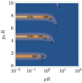
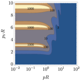
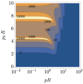
Figure 1: The uncorrected Sommerfeld enhancement factor $C_{\ell}^{2}$ for a finite square-well potential with $\ell=0$ (left panel), $\ell=1$ (middle panel), and $\ell=2$ (right panel).

The numerical value of $C_{\ell}^{2}$ is plotted in Fig. 1. We can see that $C_{\ell}^{2}$ is strongly enhanced at small velocity if $p_{V}R$ takes some specific values. This behavior comes from the existence of a zero-energy resonance. The wavefunction of the zero-energy state behaves as $u_{\ell}\propto s_{\ell}(p_{V}r)$ at $r<R$ and $u_{\ell}\propto r^{-\ell}$ at $r>R$. Then, by requiring continuity of $u_{\ell}^{\prime}/u_{\ell}$ at $r=R$, we obtain

$$J_{\ell-1/2}(p_{V}R)=0.$$ (60)

By using the Bessel function zeros $j_{n,k}$, we obtain $p_{V}R=j_{\ell-1/2,k}$ as the condition to have a zero-energy resonance. For example,

$$p_{V}R =\frac{\pi}{2},~{}\frac{3\pi}{2},~{}\frac{5\pi}{2},\cdots(\ell=0),$$ (61)

$$p_{V}R =\pi,~{}2\pi,~{}3\pi,\cdots(\ell=1),$$ (62)

$$p_{V}R =4.49,~{}7.73,~{}10.9,\cdots(\ell=2).$$ (63)

If this condition is satisfied, the low energy behavior of $C_{\ell}^{2}$ is given as follows:

$$C_{\ell}^{2}\propto\begin{cases}p^{-2}&(\ell=0)\\ p^{-4}&(\ell\geq 1)\end{cases}.$$ (64)

This behavior is consistent with the result obtained by using Levinson’s theorem and Omnès solution in Ref. Kamada:2023iol .

Now let us discuss the $\tilde{z}_{\ell}$ function. Since the potential $V(r)$ around $r=0$ is flat and there is no $1/r$ term, $x_{\ell}$ is equal to $0$ in this case. Thus, $\tilde{z}_{\ell}$ is finite in the limit $a\to 0$. By using Eq. 35, we obtain

$$\lim_{a\to 0}\tilde{z}_{\ell}(p;a)=-p^{\ell}{\tilde{p}}^{\ell+1}C_{\ell}{\rm Im}c_{F}.$$ (65)

The momentum dependence of $\tilde{z}_{\ell}$ around a zero-energy resonance is shown in the left panels of Fig. 2, and $\tilde{z}_{\ell}$ in the zero-momentum limit is shown in Fig. 3. The left panels of Fig. 2 show, if there exists a zero-energy resonance, i.e., $p_{V}R=j_{\ell-1/2,k}$ is satisfied, the low energy behavior of $\tilde{z}_{\ell}(p;0)$ is given as follows:

$$\tilde{z}_{\ell}(p;0)\propto\begin{cases}p^{0}&(\ell=0)\\ p^{-2}&(\ell\geq 1)\end{cases}$$ (66)

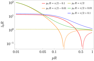
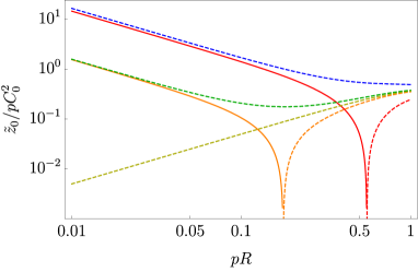
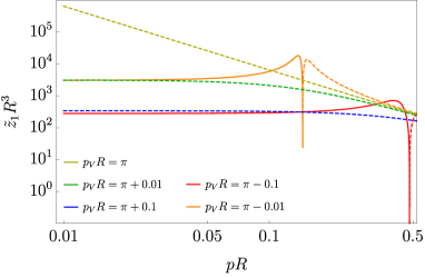
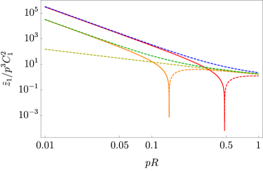
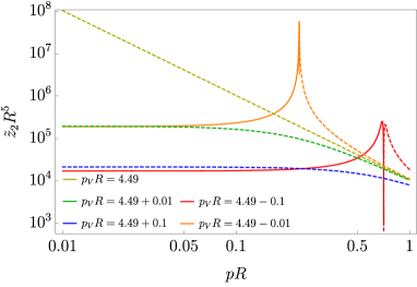
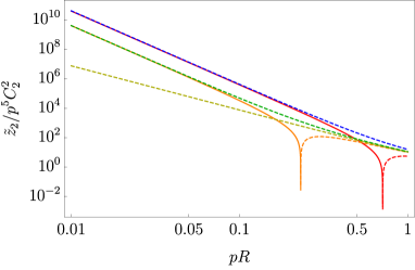
Figure 2: Left: $\tilde{z}_{\ell}(p;0)R^{2\ell+1}$ for the finite square-well potential for $\ell=0$ (upper), $\ell=1$ (middle), and $\ell=2$ (lower). Right: $\tilde{z}_{\ell}(p;0)/p^{2\ell+1}C_{\ell}^{2}$ for the finite square-well potential for $\ell=0$ (upper), $\ell=1$ (middle), and $\ell=2$ (lower). Solid (dashed) curves indicate positive (negative) $\tilde{z}_{\ell}(p;0)$.

We can see that $\tilde{z}_{\ell}(p;0)$ diverges in the limit of $p\to 0$ for $\ell\geq 1$. For the $\ell=0$ case, $\tilde{z}_{\ell}(p;0)$ does not diverge at $p=0$. However, $\tilde{z}_{\ell}(p;0)$ at small $p$ is enhanced when the parameter is slightly displaced from the zero-energy resonance. For $p_{V}R\simeq(2k-1)\pi$, $\tilde{z}_{0}(0;0)$ in the limit of $p\to 0$ behaves as

$$\tilde{z}_{0}(0;0)\simeq\frac{(2k-1)\pi}{2R}\frac{1}{p_{V}R-(2k-1)\pi}$$ (67)

Thus, $\tilde{z}_{\ell}$ is not negligible if there is a zero-energy resonance. We can define $\Delta z_{\ell}(p,p_{0})\equiv\tilde{z}_{\ell}(p)-\tilde{z}_{\ell}(p_{0})$ where $p_{0}$ is a reference momentum. Obviously, $\Delta z_{\ell}(p,p_{0})$ becomes large at low velocity if there exists a zero-energy resonance.

At the location of a zero-energy resonance with $\ell=0$, $|\tilde{z}_{0}(p;0)|$ tends to be smaller than $pC_{0}^{2}$ at low velocity; the upper right panel of Fig. 2 displays the numerical value of the ratio between $\tilde{z}_{0}$ and $pC_{0}^{2}$. We can approximate the annihilation cross section as

$$\sigma_{{\rm ann},\ell}\simeq\sigma_{{\rm ann},\ell}^{(0)}\times C_{\ell}^{2}\left|1+\frac{ipC_{0}^{2}}{k_{\ell}(p_{0})}\right|^{-2}.$$ (68)

As pointed out in Ref. Blum:2016nrz , although the conventional formula $\sigma_{{\rm ann},\ell}\simeq\sigma_{{\rm ann},\ell}^{(0)}\times C_{\ell}^{2}$ could violate the unitarity bound, the factor $\left|1+ipC_{0}^{2}/k_{\ell}(p_{0})\right|^{-2}$ in the above formula regulates the divergent behavior of the annihilation cross section. We see that $\sigma_{{\rm ann},\ell}/\sigma_{{\rm ann},\ell}^{(0)}$ becomes a momentum-independent constant in the limit $p\to 0$. On the other hand, in proximity to a zero-energy resonance with $\ell\geq 1$, $|\tilde{z}_{\ell}(p;0)|\gg p^{2\ell+1}C_{\ell}^{2}$ is satisfied at low velocity; again the ratio between $\tilde{z}_{\ell}$ and $p^{2\ell+1}C_{\ell}^{2}$ is plotted in the right panels of Fig. 2. We can approximate the annihilation cross section as

$$\sigma_{{\rm ann},\ell}\simeq\sigma_{{\rm ann},\ell}^{(0)}\times C_{\ell}^{2}\left|1+\frac{\tilde{z}_{\ell}(p;0)}{k_{\ell}(p_{0})}\right|^{-2}.$$ (69)

We can see that the factor $\left|1+\tilde{z}_{\ell}(p;0)/k_{\ell}(p_{0})\right|^{-2}$ cancels the divergent behavior of $C_{\ell}$ at low velocity, and $\sigma_{{\rm ann},\ell}/\sigma_{{\rm ann},\ell}^{(0)}$ becomes a momentum-independent constant in the limit of $p\to 0$. In Fig. 4, we show the Sommerfeld enhancement computed by the conventional formula Eq. 45, the full formula Eq. 42, and the simplified formula Eqs. 68, 69. We can see that the divergent behavior in the conventional formula (which can lead to unitarity violation) is regularized in the full formula given in Eq. 45. For the $s$-wave case, the behavior of the full formula is well captured by the simplified formula in Eq. 68. For higher partial waves, the simplified formula in Eq. 69 describes the behavior of the full formula fairly well except for the points where $\tilde{z}_{\ell}$ crosses $0$ and flips sign.

Figure 3: $|\tilde{z}_{\ell}(0;0)R^{2\ell+1}|$ for the finite square-well potential with $\ell=0$ (left), $\ell=1$ (middle), and $\ell=2$ (right). Solid (dashed) curves indicate positive (negative) $\tilde{z}_{\ell}(0;0)$.

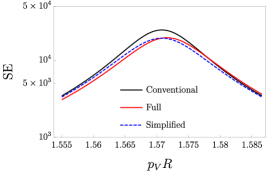
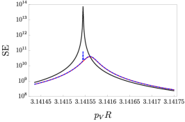
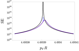
Figure 4: The ratio between the annihilation cross sections with and without the Sommerfeld effect (i.e. the Sommerfeld enhancement factor) for the finite square-well potential, for the $\ell=0$ (left), $\ell=1$ (middle) and $\ell=2$ (right) cases. The black solid curves shows the results computed using the conventional formula in Eq. 45, the red solid curves correspond to the full corrected result given in Eq. 42, and the blue dashed curves correspond to the simplified formula of Eqs. 68, 69. We take $k(p_{0})=(10^{3}+10^{3}i)R^{-1}$ for $s$-wave, $(10^{6}+10^{6}i)R^{-3}$ for $p$-wave, and $(10^{9}+10^{9}i)R^{-5}$ for $d$-wave, and choose $p=10^{-2}R^{-1}$ in all cases.

2.6.2 Coulomb potential

Let us take the attractive Coulomb potential:

$$V(r)=-\frac{1}{\mu a_{B}r}.$$ (70)

Note that $a_{B}=(\alpha\mu)^{-1}$ is the Bohr radius of this system. It is useful to define the Coulomb Hankel function:

$$H^{\pm}_{\ell}(\eta,\rho) =\frac{(\mp i)^{\ell}}{\ell!}\frac{1}{\sqrt{g_{\ell}(\eta)}C_{0}(\eta)}\Gamma(\ell+1\pm i\eta)W_{\mp i\eta,\ell+1/2}(\mp 2i\rho).$$ (71)

where $W$ is the Whittaker function, and $C_{0}$ and $g_{\ell}$ are defined as

$$C_{0}(\eta)=\sqrt{\frac{2\pi\eta}{\exp(2\pi\eta)-1}},\qquad g_{\ell}(\eta)=\prod_{k=1}^{\ell}\left(1+\frac{\eta^{2}}{k^{2}}\right).$$ (72)

Note that $C_{0}^{2}(\eta=-1/pa_{B})$ is the conventional $s$-wave Sommerfeld factor. For details, see, e.g., Ref. Gaspard:2018sqy .

The solutions of the Schrödinger equation described in Eqs. 15, 16, with boundary conditions given by Eqs. 17, 18, can be written as

$$F_{\ell}(r)={\rm Im}H_{\ell}^{+}\left(-\frac{1}{pa_{B}},pr\right),\qquad G_{\ell}(r)={\rm Re}H_{\ell}^{+}\left(-\frac{1}{pa_{B}},pr\right).$$ (73)

and we can show that the conventional Sommerfeld factor for the $\ell$-wave case is

$$C_{\ell}=\sqrt{g_{\ell}\left(-\frac{1}{pa_{B}}\right)}C_{0}\left(-\frac{1}{pa_{B}}\right).$$ (74)

Since the Coulomb potential does not have a zero-energy resonance, $C_{\ell}$ does not have a singular behavior. For $p\ll 1/a_{B}$, $C_{\ell}^{2}$ behaves as

$$C_{\ell}^{2}\simeq\frac{2\pi}{(\ell!)^{2}(pa_{B})^{2\ell+1}}.$$ (75)

We calculate $x_{\ell}(p)$ in Eq. 31 as

$$x_{\ell}(p)=-2p^{\ell-1}a_{B}^{-\ell-2}g_{\ell}\left(-\frac{1}{pa_{B}}\right).$$ (76)

and we can also calculate $\tilde{z}_{\ell}(p)$ as

$$\tilde{z}_{0}=\frac{p^{0}C_{0}}{2^{0}0!}\frac{d}{dr}G_{0}\biggr{|}_{r=a}= pa_{B}x_{0}(p)\left[\log\left(\frac{2a}{a_{B}}\right)+2\gamma_{E}+h\left(\frac{1}{pa_{B}}\right)\right],$$ (77)

$$\tilde{z}_{1}=\frac{p^{1}C_{1}}{2^{1}1!}\frac{d^{3}}{dr^{3}}r^{1}G_{1}\biggr{|}_{r=a}= p^{2}a_{B}^{2}x_{1}(p)\left[\log\left(\frac{2a}{a_{B}}\right)+2\gamma_{E}+h\left(\frac{1}{pa_{B}}\right)\right]$$

$$-\frac{p^{2}}{2a_{B}},$$ (78)

$$\tilde{z}_{2}=\frac{p^{2}C_{2}}{2^{2}2!}\frac{d^{5}}{dr^{5}}r^{2}G_{2}\biggr{|}_{r=a}= p^{3}a_{B}^{3}x_{2}(p)\left[\log\left(\frac{2a}{a_{B}}\right)+2\gamma_{E}+h\left(\frac{1}{pa_{B}}\right)\right]$$

$$-\frac{p^{2}}{16a_{B}^{3}}(4+13p^{2}a_{B}^{2}),$$ (79)

$$\tilde{z}_{3}=\frac{p^{3}C_{3}}{2^{3}3!}\frac{d^{7}}{dr^{7}}r^{3}G_{3}\biggr{|}_{r=a}= p^{4}a_{B}^{4}x_{3}(p)\left[\log\left(\frac{2a}{a_{B}}\right)+2\gamma_{E}+h\left(\frac{1}{pa_{B}}\right)\right]$$

$$-\frac{p^{2}}{48a_{B}^{5}}(2+23p^{2}a_{B}^{2}+50p^{4}a_{B}^{4}),$$ (80)

Figure 5: $\tilde{z}_{\ell}a_{B}^{2\ell+1}$ for the Coulomb potential with $\ell=0$ (left), $\ell=1$ (middle), and $\ell=2$ (right). $a$ is taken to be $10^{-5}a_{B}$ (solid curves), $10^{-10}a_{B}$ (dashed curves), and $10^{-20}a_{B}$ (dot-dashed curves).

Here $h(\eta)$ is defined as below Eq. 23. Eq. 77 shows that the $\log a$ term in $G_{\ell}$ has a momentum-independent coefficient for $\ell=0$. On the other hand, Eqs. 78–80 show the coefficient is momentum-dependent for $\ell\geq 1$ (although at least in this example, the coefficient becomes momentum-independent for $p\ll 1/a_{B}$ for general $\ell$, as $g_{\ell}(\eta)\propto\eta^{2\ell}$ for large $\eta$). Thus we cannot take the $a\to 0$ limit (and absorb the log term into the high-momentum amplitude) naively for $\ell\geq 1$ as discussed in Sec. 2.4. $\tilde{z}_{\ell}$ is constructed from a polynomial in $p$ and the function $h(1/pa_{B})$. Note that $h(\eta)$ does not have a singularity for $\eta>0$ and its asymptotic behavior is $h(\eta)\simeq-\log\eta-\gamma_{E}$ for $\eta\ll 1$ and $h(\eta)\simeq 1/12\eta^{2}$ for $\eta\gg 1$. Thus, $\tilde{z}_{\ell}$ also does not have divergent behavior at small $p$. By using dimensional analysis, $|\tilde{z}_{\ell}|$ should be bounded by $[{\rm max}(p,a_{B}^{-1})]^{2\ell+1}$. Thus, as long as the short-range effect $k_{\ell}^{-1}$ is perturbative, $|k_{\ell}|\gg|z_{\ell}|$ should be satisfied and the effect of $z_{\ell}$ is negligible. The numerical value of $\tilde{z}_{\ell}$ is shown in Fig. 5, which shows that a rough behavior of $\tilde{z}_{\ell}$ is given as

$$\tilde{z}_{\ell}\sim a_{B}^{-2\ell-1}{\rm max}[1,(pa_{B})^{2\ell}].$$ (81)

In contrast to the case of a finite square well potential, $C_{\ell}$ and $\tilde{z}_{\ell}$ do not demonstrate resonant behavior. This is the expected result because there is no zero-energy resonance in the Coulomb potential. Since $C_{\ell}$ and $\tilde{z}_{\ell}$ do not have any singular behavior, we can guarantee $|k_{\ell}(p_{0})|\gg|\Delta z(p,p_{0};a)|,~{}p^{2\ell+1}C_{\ell}^{2}$, provided the short-range physics effect can be treated perturbatively. Then we can approximate the annihilation cross section as

$$\sigma_{{\rm ann},\ell}\simeq\sigma_{{\rm ann},\ell}^{(0)}\times C_{\ell}^{2}.$$ (82)

This formula is the same as the conventional annihilation cross section formula with the Sommerfeld effect.

The scattering problem with a short-range effect and Coulomb force has been discussed in depth in the context of nuclear physics PopovMur1985 ; Carbonell:1993 ; Carbonell:1996vd ; Carbonell:1998ei ; Protasov:1999ei . In order to compare our result with those references, let us rewrite Eq. 25 by using $C_{0}$ and $g_{\ell}$ as

$$\sigma_{\text{ann},\ell}=4\pi(2\ell+1)\frac{p^{2\ell-1}g_{\ell}C_{0}^{2}{\rm Im}[-k_{\ell}^{-1}]}{|1+ip^{2\ell+1}g_{\ell}(C_{0}-ip^{-2\ell-1}g_{\ell}^{-1}\Delta z)k_{\ell}^{-1}|^{2}}.$$ (83)

Note that

$$p^{-2\ell-1}g_{\ell}^{-1}\Delta z=\frac{2}{pa_{B}}h\left(\frac{1}{pa_{B}}\right)+\cdots.$$ (84)

In the $s$-wave case, the second term of Eq. 84 does not depend on the momentum $p$. Thus, we can absorb this residual term by redefining $k_{\ell}$ and we can see that Eq. 83 is consistent with, e.g., Eq. (1) of Carbonell:1998ei . On the other hand, the second term of Eq. 84 is a polynomial in $p$ and it does depend on the momentum $p$ for $\ell\geq 1$. Thus, we cannot absorb this term by redefining a single momentum independent parameter (although we could absorb it order-by-order in $p^{2}$, by increasing the number of parameters to describe the short-range physics). This residual polynomial term is not explicitly given in Eq. (2) of Carbonell:1998ei and Eq. (2) of Protasov:1999ei , but they absorb this residual term into their definition of the short-range matrix element $K$, as discussed in Sec. 2.2. Thus, our formulation is consistent with the nuclear physics literature PopovMur1985 ; Carbonell:1993 ; Carbonell:1996vd ; Carbonell:1998ei ; Protasov:1999ei .

2.6.3 Finite range Coulomb potential

Let us take the following finite range Coulomb potential.

$$V(r)=-\frac{1}{\mu a_{B}r}\theta(R-r).$$ (85)

We assume that the effective range of the long-range force, $R$, satisfies $R>a$. This potential can be regarded as a solvable approximate description of the Yukawa potential. The solutions of the Schrödinger equation described in Eqs. 15, 16, with boundary conditions given by Eqs. 17, 18, can be written as

$$G_{\ell}+iF_{\ell}=\begin{cases}c_{G}G_{\ell}^{(C)}\left(-1/pa_{B},pr\right)+ic_{F}F_{\ell}^{(C)}\left(-1/pa_{B},pr\right)&(r<R)\\ \exp\left(i\delta_{\ell}^{(L)}\right)[c_{\ell}(pr)+is_{\ell}(pr)]&(r\geq R)\end{cases}.$$ (86)

Here we use the $(C)$ superscript to indicate results from the Coulomb potential without a cutoff. Note that ${\rm Im}c_{G}=0$ and ${\rm Re}c_{F}=1/c_{G}$ can be shown by using the boundary conditions Eq. 17 and Eq. 18, respectively. The continuity of $G_{\ell}+iF_{\ell}$ and $G^{\prime}_{\ell}+iF^{\prime}_{\ell}$ at $r=R$ imposes:

$$c_{F} =\exp\left(i\delta_{\ell}^{(L)}\right)\left(i\frac{1}{p}\frac{dG_{\ell}^{(C)}}{dr}(c_{\ell}+is_{\ell})-iG_{\ell}^{(C)}(c^{\prime}_{\ell}+is^{\prime}_{\ell})\right)\biggr{|}_{r=R},$$ (87)

$$c_{G} =\exp\left(i\delta_{\ell}^{(L)}\right)\left(\frac{1}{p}\frac{dF_{\ell}^{(C)}}{dr}(c_{\ell}+is_{\ell})-F_{\ell}^{(C)}(c^{\prime}_{\ell}+is^{\prime}_{\ell})\right)\biggr{|}_{r=R}.$$ (88)

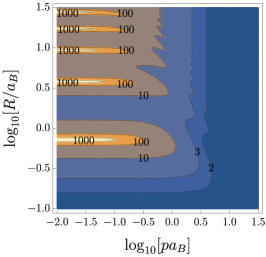
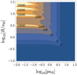
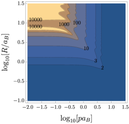
Figure 6: The conventional Sommerfeld factor $C_{\ell}^{2}$ for a finite-range Coulomb potential (set to zero for $r>R$) for $\ell=0$ (left), $\ell=1$ (middle), and $\ell=2$ (right).

The phase shift $\delta_{\ell}^{(L)}$ and Sommerfeld factor $C_{\ell}^{2}$ are calculated as

$$\delta_{\ell}^{(L)} =-{\rm arg}\left(\frac{1}{p}\frac{dF_{\ell}^{(C)}}{dr}(c_{\ell}+is_{\ell})-F_{\ell}^{(C)}(c^{\prime}_{\ell}+is^{\prime}_{\ell})\right)\biggr{|}_{r=R},$$ (89)

$$C_{\ell}^{2} =\frac{|C_{\ell}^{(C)}|^{2}}{|c_{G}|^{2}}=|C_{\ell}^{(C)}|^{2}\left|\frac{1}{p}\frac{dF_{\ell}^{(C)}}{dr}(c_{\ell}+is_{\ell})-F_{\ell}^{(C)}(c^{\prime}_{\ell}+is^{\prime}_{\ell})\right|^{-2}_{r=R}.$$ (90)

The numerical values of the unregulated Sommerfeld enhancement $C_{\ell}^{2}$ are shown in Fig. 6. Similarly to the spherical well potential discussed in Sec. 2.6.1, $C_{\ell}$ is strongly enhanced at small velocity if $R/a_{B}$ takes specific values; this is the standard zero-energy resonance behavior.

The wavefunction of a zero-energy state behaves as $u_{\ell}\propto\sqrt{r}J_{2\ell+1}(2\sqrt{2r/a_{B}})$ at $r<R$ and $u_{\ell}\propto r^{-\ell}$ at $r>R$. Then, by requiring continuity of $u^{\prime}_{\ell}/u_{\ell}$ at $r=R$, we obtain

$$\,{}_{0}F_{1}\!\left(2\ell+1,-\frac{2R}{a_{B}}\right)=0$$ (91)

where $\,{}_{0}F_{1}(a,b)$ is the confluent hypergeometric function. A few numerical solutions of this condition are

$$\frac{R}{a_{B}} =0.723,~{}3.81,~{}9.36,~{}\cdots(\ell=0),$$ (92)

$$\frac{R}{a_{B}} =3.30,~{}8.86,~{}16.9,~{}\cdots(\ell=1),$$ (93)

$$\frac{R}{a_{B}} =7.20,~{}15.3,~{}25.8,~{}\cdots(\ell=2).$$ (94)

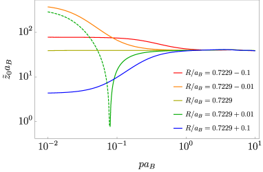
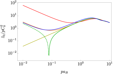
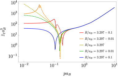
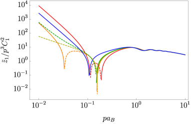
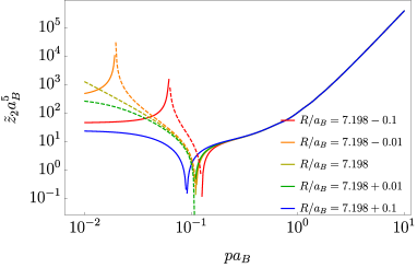
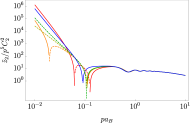
Figure 7: Left: $\tilde{z}_{\ell}a_{B}^{2\ell+1}$ as a function of $p$ for the finite-range Coulomb potential for $\ell=0$ (upper), $\ell=1$ (middle), and $\ell=2$ (lower). We take $a=10^{-10}a_{B}$. Right: $\tilde{z}_{\ell}(p;0)/p^{2\ell+1}C_{\ell}^{2}$ for the finite-range Coulomb potential for $\ell=0$ (upper), $\ell=1$ (middle), and $\ell=2$ (lower). We take $a=10^{-10}a_{B}$. Solid (dashed) curves indicate positive (negative) values of $\tilde{z}_{\ell}$.

If this condition is satisfied, the low energy behavior of $C_{\ell}^{2}$ is given as follows:

$$C_{\ell}^{2}\propto\begin{cases}p^{-2}&(\ell=0)\\ p^{-4}&(\ell\geq 1)\end{cases}.$$ (95)

As in the square-well potential case, this behavior is consistent with the result obtained by using Levinson’s theorem and Omnès solution in Ref. Kamada:2023iol .

An explicit calculation shows

$$x_{\ell}(p)=\frac{c_{G}C_{\ell}}{C_{\ell}^{(C)}}x_{\ell}^{(C)}(p)=x_{\ell}^{(C)}(p).$$ (96)

We can see that $x_{\ell}(p)$ is the same as the Coulomb potential because $x_{\ell}(p)$ is determined by the recursion relations at the origin, as shown in Eq. 184. As shown in Eq. 35, the $a$-dependence in $\tilde{z}_{\ell}$ is determined by $x_{\ell}$. Thus, we can expect that $z_{\ell}$ has a similar term to $z_{\ell}^{(C)}$ and can explicitly show that

$$\tilde{z}_{\ell}=\frac{p^{\ell}C_{\ell}}{2^{\ell}\ell!}\frac{d^{2\ell+1}}{dr^{2\ell+1}}G_{\ell}\biggr{|}_{r=a} =-{\rm Im}c_{F}C_{\ell}C_{\ell}^{(C)}p^{2\ell+1}+c_{G}\frac{p^{\ell}C_{\ell}}{2^{\ell}\ell!}\frac{d^{2\ell+1}}{dr^{2\ell+1}}G_{\ell}^{(C)}\biggr{|}_{r=a}$$

$$=-{\rm Im}c_{F}C_{\ell}C_{\ell}^{(C)}p^{2\ell+1}+\tilde{z}_{\ell}^{(C)}.$$ (97)

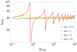
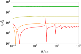
Figure 8: $\tilde{z}_{\ell}a_{B}^{2\ell+1}$ as a function of $R$ for the finite-range Coulomb potential with $\ell=0$ (left), $\ell=1$ (middle), and $\ell=2$ (right). We show results for several different values of the momentum: $p=0.1a_{B}^{-1}$ (red curves), $a_{B}^{-1}$ (orange curves), $3a_{B}^{-1}$ (yellow curves), and $10a_{B}^{-1}$ (green curves). We take $a=10^{-10}a_{B}$. Solid (dashed) curves indicate positive (negative) values of $\tilde{z}_{\ell}$.

Note that we have used $c_{G}C_{\ell}=C_{\ell}^{(C)}$. The $a$-dependent term in $\tilde{z}_{\ell}$ is the second term of the RHS, $\tilde{z}_{\ell}^{(C)}$. Since the coefficient of the $\log a$ term depends on $p$ for $\ell\geq 1$ (at least for $p\gtrsim 1/a_{B}$), we cannot absorb $\log a$ dependent terms into a momentum independent constant $k_{\ell}$ for $\ell\geq 1$. Fig. 7 and Fig. 8 show that, if there exists a zero-energy resonance, i.e., $\,{}_{0}F_{1}\!\left(2\ell+1,-2R/a_{B}\right)=0$ is satisfied, the low energy behavior of $\tilde{z}_{\ell}$ is given as follows:

$$\tilde{z}_{\ell}\propto\begin{cases}p^{0}&(\ell=0)\\ p^{-2}&(\ell\geq 1)\end{cases}.$$ (98)

We can see $\tilde{z}_{\ell}$ diverges in the limit of $p\to 0$ for $\ell\geq 1$. For the $\ell=0$ case, $\tilde{z}_{\ell}$ does not diverge at $p=0$, however, $\tilde{z}_{\ell}$ at small $p$ is enhanced when the parameter is slightly displaced from the zero-energy resonance. Thus, $\tilde{z}_{\ell}$ is not negligible if there is a zero-energy resonance. We can define $\Delta z_{\ell}(p,p_{0})\equiv\tilde{z}_{\ell}(p)-\tilde{z}_{\ell}(p_{0})$ where $p_{0}$ is a reference momentum. Obviously, $\Delta z_{\ell}(p,p_{0})$ becomes large at low velocity if there exists a zero-energy resonance.

The behavior of the annihilation cross section in proximity to a zero-energy resonance is similar to the square-well potential case. For $\ell=0$, we can assume $|\tilde{z}_{0}|\ll pC_{0}^{2}$ at low velocity; see the upper right panel of Fig. 7 for the numerical value of the ratio between $\tilde{z}_{0}$ and $pC_{0}^{2}$. We obtain

$$\sigma_{{\rm ann},\ell}\simeq\sigma_{{\rm ann},\ell}^{(0)}\times C_{\ell}^{2}\left|1+\frac{ipC_{0}^{2}}{k_{\ell}(p_{0})}\right|^{-2}.$$ (99)

For $\ell\geq 1$, we can assume $|\tilde{z}_{\ell}|\gg p^{2\ell+1}C_{\ell}^{2}$ at low velocity. See the right panels of Fig. 7 for numerical value of the ratio between $\tilde{z}_{\ell}$ and $p^{2\ell+1}C_{\ell}^{2}$. We obtain

$$\sigma_{{\rm ann},\ell}\simeq\sigma_{{\rm ann},\ell}^{(0)}\times C_{\ell}^{2}\left|1+\frac{\Delta z_{\ell}(p;p_{0})}{k_{\ell}(p_{0})}\right|^{-2}.$$ (100)

In both the $\ell=0$ and $\ell\geq 1$ cases, the divergent behavior of $C_{\ell}^{2}$ as $p\rightarrow 0$ is suppressed by the last factor on the right-hand side of this equation. In Fig. 9, we show the Sommerfeld enhancement as calculated by the conventional formula Eq. 45, the full formula Eq. 42, and the simplified formula Eqs. 99, 100. For the $s$-wave case, the behavior of the full formula is well captured by the simplified formula Eq. 99. For higher partial waves, the simplified formula Eq. 100 describes the behavior of the full formula fairly well, except for the points where $\tilde{z}_{\ell}$ crosses $0$ and flips its sign; these behaviors are similar to those for the finite square well.

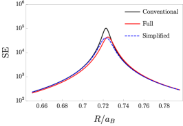
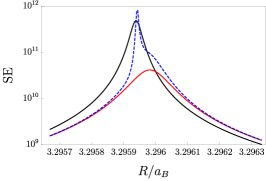
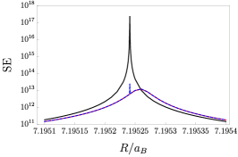
Figure 9: The ratio between the annihilation cross sections with and without the Sommerfeld effect for the finite-range Coulomb potential, for the $\ell=0$ (left), $\ell=1$ (middle) and $\ell=2$ (right) cases. The black solid curves shows the results computed using the conventional formula in Eq. 45, the red solid curves correspond to the full corrected result given in Eq. 42, and the blue dashed curves correspond to the simplified formula of Eqs. 99, 100. We take $k(p_{0})=(10^{3}+10^{3}i)a_{B}^{-1}$ for the $s$-wave case, $(10^{5}+10^{5}i)a_{B}^{-3}$ for the $p$-wave case, and $(10^{5}+10^{5}i)a_{B}^{-5}$ for the $d$-wave case. We choose $p=10^{-2}a_{B}^{-1}$ and $a=10^{-10}a_{B}$ in all cases.

3 The multi-state case for general $\ell$

In general, the long-range potential may couple a number of two-body states, and the short-range annihilation may proceed through any of these states. Scenarios with multiple interacting nearly-degenerate states were already considered in the first works on Sommerfeld enhancement as applied to dark matter annihilation Hisano:2002fk ; Hisano:2003ec ; Hisano:2004ds , and methods for the standard (uncorrected) Sommerfeld calculation are well-developed for multi-state systems.

Assuming the energy associated with the potential to be small compared to the mass, we will generally treat all states that can be excited due to the potential as having approximately equal masses $M$, and treat the mass differences between them as terms in the potential. In this case, $V_{\text{long}}(r)$ is a matrix describing the potential, and its diagonal elements include terms for the mass splittings between states, as in e.g. Hisano:2004ds .

The states coupled by the potential may or may not be kinematically accessible at large distances, depending on the velocity of the interacting particles; we will consider the general case where there are $N$ coupled two-body states, and $M$ of these are kinematically accessible. If the 3-momentum of a single particle in the lowest-mass state is defined to be $p$, and the reduced mass of the system is $\mu$, we can define the single-particle momentum in the $n$th two-body state as follows, by energy conservation:

$$p_{n}\equiv\sqrt{p^{2}-2\mu\mathrm{lim}_{r\rightarrow\infty}V_{\text{long},nn}(r)},$$ (101)

where now $p_{n}$ is real for the $M$ kinematically accessible states and imaginary otherwise.

We will assume throughout this section that the potential is spherically symmetric and ignore couplings between states of different $\ell$. Then the Schrödinger equation satisfied by the $\ell$th partial wave of the component of the radial reduced wavefunction in the $n$th state can be written:

$$\left[\left(-\frac{d^{2}}{dr^{2}}+\frac{\ell(\ell+1)}{r^{2}}-p_{a}^{2}\right)\delta_{ab}+2\mu(\hat{V}_{\text{long}}(r))_{ab}\right]u_{b}(r)=0,$$ (102)

where $\hat{V}_{\text{long}}(r)$ is a $N\times N$ matrix that goes to zero as $r\rightarrow\infty$. We will assume throughout that $V_{\text{long}}(r)$ (and hence $\hat{V}_{\text{long}}(r)$) is real and symmetric for all $r$.

3.1 The two-body scattering problem for multiple states

The contribution to the wavefunction corresponding to scattering from such a potential is given asymptotically by $(\psi_{n}({\bf x}))_{\mathrm{scattered}}\rightarrow f_{n}(\theta)e^{ip_{n}r}/r$, for $n=1,\ldots,M$ (again, only the first $M$ states are kinematically allowed at large $r$). Performing the partial wave expansion for a plane wave $e^{ipz}$ as previously, and defining $f_{n}(\theta)=\sum_{\ell}(2\ell+1)f_{nl}P_{\ell}(\cos\theta)$, we can write, for $n=1,\ldots,M$:

$$\psi_{n}(r,\theta)\rightarrow(2\ell+1)P_{l}(\cos\theta)\left[a_{n}\frac{e^{ip_{n}r}-(-1)^{\ell}e^{-ip_{n}r}}{2ip_{n}r}+f_{n\ell}\frac{e^{ip_{n}r}}{r}\right].,$$ (103)

where the $a_{n}$ coefficients describe the two-body state for the incoming particles at large $r$. For states with $n>M$, where $p_{n}$ is imaginary, we can use a similar expansion, but with $a_{n}=0$ (corresponding to the fact that there is no incoming plane wave in this state); the purely-outgoing $f_{nl}$ component then translates into an exponentially suppressed component, as required to have a physical solution.

Consider the solution of the Schrödinger equation where the initial unscattered plane wave corresponds entirely to a single two-body state (labeled $i$, $i=1,\ldots,M$), i.e. we can write $a_{n}=\delta_{ni}$ where $i$ runs from 1 to $M$, and so the incoming particles each carry momentum $p_{i}$. Let $f_{ni\ell}$ be defined as $f_{n\ell}$ when the initial state is purely the $i$th state; when we write $f_{\ell}$, we will henceforth mean the $N\times M$ matrix with elements $f_{ni\ell}$. The scattering amplitude from the $i$th kinematically allowed state to the $n$th kinematically allowed state will be given by the truncation of $f_{\ell}$ to $M\times M$.

The form of the $n$-component of the wavefunction at large $r$, for an initial plane-wave in component $i$, will be:

$$\psi_{ni}(r,\theta) \rightarrow(2\ell+1)P_{l}(\cos\theta)\left[\delta_{ni}\frac{e^{ip_{n}r}-(-1)^{l}e^{-ip_{n}r}}{2ip_{n}r}+f_{ni\ell}\frac{e^{ip_{n}r}}{r}\right]$$

$$\sim(2\ell+1)P_{l}(\cos\theta)e^{i\pi\ell/2}\frac{1}{p_{n}r}\left[\left(\delta_{ni}+ip_{n}f_{ni\ell}\right)s_{\ell}(p_{n}r)+f_{ni\ell}p_{n}c_{\ell}(p_{n}r)\right].$$ (104)

We can define a reduced wavefunction vector, with $n$-component $u_{ni\ell}(r)$, that is directly proportional to $r\psi_{ni}(r,\theta)$ with a proportionality factor that depends only on $\ell,\theta$ and $p_{i}$; for consistency with the one-state case, we will choose the reduced wavefunction to have the large-$r$ asymptotics:

$$u_{ni\ell}(r)\rightarrow\frac{p_{i}}{p_{n}}\left[\left(\delta_{ni}+ip_{n}f_{ni\ell}\right)s_{\ell}(p_{n}r)+f_{ni\ell}p_{n}c_{\ell}(p_{n}r)\right]=\left(\delta_{ni}+ip_{i}f_{ni\ell}\right)s_{\ell}(p_{n}r)+f_{ni\ell}p_{i}c_{\ell}(p_{n}r).$$ (105)

In the unperturbed case we see that $u_{ni\ell}(r)\rightarrow\delta_{ni}s_{\ell}(p_{n}r)$ at large $r$.

In this case, the incident probability flux is $\langle J_{\mathrm{in}}\rangle=p_{i}/\mu$. The scattered flux into a (kinematically allowed) state with momentum $p_{f}$, where $p_{f}$ is real ($f=1,\ldots,M$), is given by $\langle J_{\mathrm{out}}\rangle=\frac{p_{f}}{\mu}\frac{1}{r^{2}}|f_{fi}(\theta)|^{2}$, where $f_{fi}(\theta)=\sum_{l}(2\ell+1)f_{fi\ell}P_{l}(\cos\theta)$. The cross section for this scattering process is given by:

$$\frac{d\sigma_{i\rightarrow f}}{d\Omega}=r^{2}\frac{\langle J_{\mathrm{out}}\rangle}{\langle J_{\mathrm{in}}\rangle}=\frac{p_{f}}{p_{i}}\left|\sum_{l}(2l+1)f_{fi\ell}P_{l}(\cos\theta)\right|^{2}.$$ (106)

Performing the angular integral using the orthogonality of the Legendre polynomials, we obtain the scattering cross sections:

$$\sigma_{i\rightarrow f}=4\pi\frac{p_{f}}{p_{i}}\sum_{l}(2l+1)\left|f_{fi\ell}\right|^{2}=\pi\frac{1}{p_{i}^{2}}\sum_{l}(2l+1)\left|S_{fi\ell}-\delta_{fi}\right|^{2},$$ (107)

where we have defined the normalized $S$-matrix $S_{fi\ell}\equiv\delta_{fi}+2if_{fi\ell}\sqrt{p_{i}p_{f}}$. This choice ensures that the probability conservation condition remains $S_{\ell}^{\dagger}S_{\ell}=1$, in the absence of absorptive processes such as annihilation. Considering $S_{fi\ell}$ and $f_{fi\ell}$ as the $(f,i)$ components of matrices $S_{\ell}$ and $f_{\ell}$, we observe that $S_{\ell}$ is a $M\times M$ matrix, describing scattering from one kinematically allowed two-body state to another kinematically allowed two-body state.

The annihilation cross section, for the $i$th initial state, can be derived from the apparent non-conservation of the probability current and is given by:

$$\sigma_{i,\mathrm{ann}}=\frac{\pi}{p_{i}^{2}}\sum_{l}(2\ell+1)\left(1-\sum_{f}|S_{fi\ell}|^{2}\right)=\frac{\pi}{p_{i}^{2}}\sum_{\ell}(2\ell+1)\left(1-S_{\ell}^{\dagger}S_{\ell}\right)_{ii}.$$ (108)

As in Sec. 2, this relation assumes distinguishable particles in the initial state, and should be corrected by a prefactor $c_{i}$ which is 1 for distinguishable particles and 2 for identical particles. We will generally work with scattering amplitudes appropriate for distinguishable particles unless noted otherwise (see App. C for a discussion of how to obtain the correctly rescaled matrix elements from QFT for short-distance scattering amplitudes involving identical particles).

For the remainder of this section, we will generally suppress $\ell$ subscripts when writing out the components of objects that carry state indices, in an attempt to simplify the notation. All wavefunctions, $S$-matrix elements, cross sections, etc., are separated into partial waves (and thus carry an implicit $\ell$ index) unless explicitly noted otherwise. We will make the $\ell$ indices explicit when dealing with the objects themselves rather than their components, e.g. we will write $S_{\ell}$ for the $S$-matrix but $S_{fi}$ for its components.

3.2 Constructing the wavefunction with modified short-range physics

Our goal now is to relate $f_{\ell}$ and $S_{\ell}$ to the Sommerfeld enhancement arising from the long-range potential for $r>a$ (obtained from the regular solution to the long-range Schrödinger equation), and the modification of the boundary condition at $r=a$ due to short-range physics. The results of this section will generalize our one-state results from Sec. 2.

Let us decompose the reduced wavefunction for $r>a$, whose components we denote $u_{ni}(r)$, into the regular solution to the long-range Schrödinger equation, denoted $w_{ni}(r)$ (with the standard boundary conditions as $r\rightarrow 0$), and a correction associated with the short-range physics. As previously, $i$ indexes the initial state and $n$ indexes the wavefunction component. We choose $w_{ni}(r)$ and $u_{ni}(r)$ to correspond to the same ingoing plane wave (i.e. in the $i$th state and with standard normalization), so that $u_{ni}(r)\rightarrow w_{ni}(r)$ for $r>a$ in the limit where the long-range potential is the only relevant physics, and in general $u_{ni}(r)-w_{ni}(r)$ is purely outgoing at large $r$. We can write this purely-outgoing component as a linear combination of basis solutions,

$$u_{ni}(r)=w_{ni}(r)+\tilde{w}_{nj}(r)R_{ji},$$ (109)

where we define the basis wavefunctions $\tilde{w}_{nj}(r)$ as the unique irregular solutions to the long-range Schrödinger equation that are purely outgoing (or exponentially suppressed) at infinity, and whose leading-order short-distance behavior is:

$$\tilde{w}_{nj}(r)\rightarrow\delta_{nj}(2\ell-1)!!r^{-\ell}\,\,\text{as}\,r\rightarrow 0.$$ (110)

The constant coefficients $R_{ji}$ (which collectively inhabit a matrix $R_{\ell}$) should be chosen to fix the desired boundary conditions at $r=a$, and thus will be determined by the short-distance physics combined with the properties of the $w_{ni}(r)$ and $\tilde{w}_{ni}(r)$ solutions as $r\rightarrow a$. Note that we must allow $j$ to take values from $1$ to $N$, not solely $1$ to $M$, to allow for cases where there is a non-trivial short-distance boundary condition in a component that is kinematically suppressed at large $r$.

3.3 Properties of the basis solutions

Solutions similar to $\tilde{w}_{nj}(r)$ have been studied previously (e.g. in Ref. Slatyer:2009vg ); because the boundary conditions here are slightly modified, and for completeness, we repeat some calculations of key properties here. For this section, we will only need to consider the standard long-range Schrödinger equation, in the range $0<r<\infty$, without any short-distance perturbations. Because we treat the potential as fully general (beyond the assumption that it is real and symmetric), this covers our full range of conventions for $V_{\text{long}}(r)$ at $r<a$.

Assuming the long-distance potential is real, the real and imaginary parts of $\tilde{w}_{ni}(r)$ are independently (real) solutions of the Schrödinger equation (with the long-distance potential). Let us write $\tilde{w}_{ni}(r)=\tilde{G}_{ni}(r)+i\tilde{F}_{ni}(r)$, with $\tilde{G}_{\ell}$ and $\tilde{F}_{\ell}$ being real functions with components $\tilde{G}_{ni}$, $\tilde{F}_{ni}$ respectively (similarly to the one-state case, but note the normalization convention is different here, to avoid having to deal with the question of whether factors of the momentum are real or imaginary). Note also that by our choice of boundary condition, $\tilde{F}_{ni}(r)$ is a regular solution to the long-range Schrödinger equation (for the reduced wavefunction), i.e. it vanishes at the origin. Then the boundary conditions on $\tilde{F}_{\ell}$ and $\tilde{G}_{\ell}$ as $r\rightarrow 0$ can be written:

$$\tilde{G}_{ni}(r) \rightarrow\delta_{ni}(2\ell-1)!!r^{-\ell},\quad\tilde{F}_{ni}(r)\rightarrow(z_{ni}/p_{n}^{\ell+1})s_{\ell}(p_{n}r),\quad r\rightarrow 0.$$ (111)

where $z_{ni}$ denotes the components of a real $N\times N$ matrix.

For the boundary condition at large $r$, since $\tilde{w}_{nj}(r)$ is purely outgoing at large $r$, we can define the components of a constant matrix $f_{1,\ell}$ by:

$$\tilde{w}_{nj}(r)\rightarrow p_{j}f_{1,nj}(c_{\ell}(p_{n}r)+is_{\ell}(p_{n}r)),\quad r\rightarrow\infty.$$ (112)

Thus we obtain the following conditions on $\tilde{G}_{\ell}$ and $\tilde{F}_{\ell}$ at large $r$:

$$\tilde{G}_{ni}(r) \rightarrow\text{Re}(p_{i}f_{1,ni}c_{\ell}(p_{n}r))-\text{Im}(p_{i}f_{1,ni}s_{\ell}(p_{n}r)),$$

$$\tilde{F}_{ni}(r) \rightarrow\text{Re}(p_{i}f_{1,ni}s_{\ell}(p_{n}r))+\text{Im}(p_{i}f_{1,ni}c_{\ell}(p_{n}r)),\quad r\rightarrow\infty.$$ (113)

Let $f_{0,\ell}$ (with components denoted $f_{0,ni}$) be the scattering amplitude for the $w_{ni}(r)$ solution (i.e. the scattering amplitude from the long-range potential with no short-distance physics), and let the short-distance behavior of $w_{ni}(r)$ be given by:

$$w_{ni}(r) \rightarrow Q_{ni}s_{\ell}(p_{n}r).$$ (114)

Let us first consider the Wronskian computed from the regular solution $w_{\ell}$ (with components $w_{ni}$) and the irregular solution $\tilde{w}_{\ell}=\tilde{G}_{\ell}+i\tilde{F}_{\ell}$, in the form $W_{ij}=(w_{\ell}^{T}\tilde{w}^{\prime}_{\ell}-w^{T\prime}_{\ell}\tilde{w}_{\ell})_{ij}=\sum_{n}w_{ni}\tilde{w}_{nj}^{\prime}-\sum_{n}w_{ni}^{\prime}\tilde{w}_{nj}$. Using the small-distance asymptotic behavior of $s_{\ell}(x)$ and $c_{\ell}(x)$, we observe:

$$W_{ij}(r\rightarrow 0) =\sum_{n}Q_{ni}\frac{1}{(2\ell+1)!!}(p_{n}r)^{\ell+1}\delta_{nj}(2\ell-1)!!(-\ell)r^{-\ell-1}$$

$$-\sum_{n}Q_{ni}\frac{1}{(2\ell+1)!!}p_{n}(\ell+1)(p_{n}r)^{\ell}\delta_{nj}(2\ell-1)!!r^{-\ell}$$

$$=-Q_{ji}p_{j}^{\ell+1}.$$ (115)

Then for the Wronskian we obtain:

$$W_{ij}(r\rightarrow\infty) =\sum_{n\leq M}(\delta_{ni}s_{\ell}(p_{n}r)+p_{i}f_{0,ni}(c_{\ell}(p_{n}r)+is_{\ell}(p_{n}r)))f_{1,nj}p_{j}p_{n}(-s_{\ell}(p_{n}r)+ic_{\ell}(p_{n}r))$$

$$-(\delta_{ni}p_{n}c_{\ell}(p_{n}r)+p_{i}p_{n}f_{0,ni}(-s_{\ell}(p_{n}r)+ic_{\ell}(p_{n}r)))f_{1,nj}p_{j}(c_{\ell}(p_{n}r)+is_{\ell}(p_{n}r))$$

$$=-f_{1,ij}p_{j}p_{i}.$$ (116)

Thus, constancy of the Wronskian (which follows from the Schrödinger equation) implies $Q_{ji}p_{j}^{\ell+1}=f_{1,ij}p_{j}p_{i}$, or $f_{1,ij}=(p_{j}^{\ell}/p_{i})Q_{ji}$.

We can also compute the large-$r$ and small-$r$ limits of the Wronskian derived from treating $\tilde{G}_{\ell}$ and $\tilde{F}_{\ell}$ as independent solutions, $\tilde{W}_{ij}=(\tilde{G}_{\ell}^{T}\tilde{F}_{\ell}^{\prime}-\tilde{G}^{T\prime}_{\ell}\tilde{F}_{\ell})_{ij}$, and from invariance of the Wronskian. We obtain:

$$\tilde{W}_{ij}(r\rightarrow 0) =z_{ij},$$

$$\tilde{W}_{ij}(r\rightarrow\infty) =\sum_{n\leq M}p_{n}(\text{Re}(p_{i}f_{1,ni})\text{Re}(p_{j}f_{1,nj})+\text{Im}(p_{i}f_{1,ni})\text{Im}(p_{j}f_{1,nj})),$$

$$\Rightarrow z_{ij} =\sum_{n\leq M}\frac{1}{p_{n}}(\text{Re}(p_{i}^{\ell+1}Q_{in})\text{Re}(p_{j}^{\ell+1}Q_{jn})+\text{Im}(p_{i}^{\ell+1}Q_{in})\text{Im}(p_{j}^{\ell+1}Q_{jn})).$$ (117)

where only the states with $n\leq M$ contribute in the calculation of $\tilde{W}_{ij}(r\rightarrow\infty)$ as the others are exponentially suppressed as $r\rightarrow\infty$.

For convenience, we can define $\bar{Q}_{\ell}$ as a $N\times M$ matrix with elements $\bar{Q}_{in}=p_{i}^{\ell+1}Q_{in}/\sqrt{p_{n}}$, and then write:

$$z_{ij} =\sum_{n\leq M}(\text{Re}\bar{Q}_{in})(\text{Re}\bar{Q}_{jn})+(\text{Im}\bar{Q}_{in})(\text{Im}\bar{Q}_{jn})=\text{Re}(\bar{Q}_{\ell}\bar{Q}_{\ell}^{\dagger})_{ij}.$$ (118)

We can do one further Wronskian calculation to relate $f_{0,\ell}$ to $Q_{\ell}$, this time computing $\hat{W}_{ij}=(w^{\dagger}_{\ell}\tilde{w}^{\prime}_{\ell}-w^{\dagger\prime}_{\ell}\tilde{w}_{\ell})_{ij}=\sum_{n}w_{ni}^{*}\tilde{w}_{nj}^{\prime}-\sum_{n}w_{ni}^{*\prime}\tilde{w}_{nj}$, where $i$ runs from 1 to $M$ and $j$ runs from 1 to $N$. Now at short distances we obtain:

$$\hat{W}_{ij}(r\rightarrow 0) =\sum_{n}Q_{ni}^{*}\frac{1}{(2\ell+1)!!}(p_{n}^{*}r)^{\ell+1}\delta_{nj}(2\ell-1)!!(-\ell)r^{-\ell-1}$$

$$-\sum_{n}Q_{ni}^{*}\frac{1}{(2\ell+1)!!}p_{n}^{*}(\ell+1)(p_{n}^{*}r)^{\ell}\delta_{nj}(2\ell-1)!!r^{-\ell}$$

$$=-Q_{ji}^{*}(p_{j}^{*})^{\ell+1}.$$ (119)

At large distances, we have:

$$\hat{W}_{ij}(r\rightarrow\infty) =\sum_{n\leq M}(\delta_{ni}s_{\ell}(p_{n}r)+p_{i}f^{*}_{0,ni}(c_{\ell}(p_{n}r)-is_{\ell}(p_{n}r)))if_{1,nj}p_{j}p_{n}(c_{\ell}(p_{n}r)+is_{\ell}(p_{n}r))$$

$$-(\delta_{ni}p_{n}c_{\ell}(p_{n}r)-ip_{i}p_{n}f^{*}_{0,ni}(c_{\ell}(p_{n}r)-is_{\ell}(p_{n}r))f_{1,nj}p_{j}(c_{\ell}(p_{n}r)+is_{\ell}(p_{n}r))$$

$$=-f_{1,ij}p_{j}p_{i}+2ip_{i}p_{j}\sum_{n\leq M}f^{*}_{0,nil}p_{n}f_{1,nj}.$$ (120)

From our previous result that $Q_{ji}p_{j}^{\ell+1}=f_{1,ij}p_{j}p_{i}$, constancy of the Wronskian implies:

$$-Q_{ji}^{*}(p_{j}^{*})^{\ell+1} =-Q_{ji}p_{j}^{\ell+1}+2ip_{i}p_{j}^{\ell+1}\sum_{n\leq M}f^{*}_{0,ni}Q_{jn},$$

$$\Rightarrow\frac{\bar{Q}_{ji}-\bar{Q}_{ji}^{*}}{2i} =\sum_{n\leq M}\sqrt{p_{i}p_{n}}f^{*}_{0,ni}\bar{Q}_{jn}.$$ (121)

3.4 Extracting the modified $S$-matrix element

Now we can use the properties derived in the previous subsection to write down expressions for the $S$-matrix element in the presence of additional short-distance physics. We can read off the full scattering amplitude, $f_{\ell}$ (with components denoted $f_{ni}$), from the long-range behavior of $u_{ni}(r)$, obtaining a contribution from $w_{ni}(r)$ which is identical to that in the case with no short-range physics, and then an additional contribution from the purely-outgoing $\tilde{w}$ term:

$$f_{ni}=f_{0,ni}+f_{1,nj}(p_{j}/p_{i})R_{ji}.$$ (122)

In turn, we can write the full $S$-matrix element as:

$$S_{ni}=S_{0,ni}+2if_{1,nj}(p_{j}/p_{i})R_{ji}\sqrt{p_{i}p_{n}}=S_{0,ni}+2i(p_{j}^{\ell+1})Q_{jn}R_{ji}/\sqrt{p_{n}p_{i}},$$ (123)

where $S_{0,ni}=\delta_{ni}+2if_{0,ni}\sqrt{p_{i}p_{n}}$ is the $S$-matrix corresponding to scattering through the long-range potential only. $n$ and $i$ take values from 1 to $M$, whereas $j$ runs from 1 to $N$.

It is also helpful to define a complex $N\times N$ diagonal matrix $\tilde{P}$ with elements $\tilde{P}_{ij}=\sqrt{p_{i}}\delta_{ij}$; we denote by $P$ the (real) truncation of $\tilde{P}$ to the $M\times M$ subspace. Then in matrix form (and noting that $R$ is $N\times M$), we can write:

$$S_{\ell}=S_{0,\ell}+2i\bar{Q}^{T}_{\ell}R_{\ell}P^{-1}.$$ (124)

Thus we have reduced the problem of computing the full $S$-matrix element to that of computing $S_{0,\ell}$, $\bar{Q}_{\ell}$ and the coefficients in the matrix $R_{\ell}$. $S_{0,\ell}$ and $\bar{Q}_{\ell}$ can be computed using standard methods from the Schrödinger equation with only the long-distance potential. We can also use Eq. 121 to relate these quantities:

$$\frac{\bar{Q}_{ji}-\bar{Q}_{ji}^{*}}{2i}=\sum_{n\leq M}\left(\frac{S_{0,ni}-\delta_{ni}}{2i}\right)^{*}\bar{Q}_{jn},$$ (125)

or in matrix form,

$$\bar{Q}^{T}_{\ell}-\bar{Q}^{\dagger}_{\ell} =-(S_{0,\ell}-1)^{\dagger}\bar{Q}_{\ell}^{T}\Rightarrow\bar{Q}_{\ell}^{*}S_{0,\ell}=\bar{Q}_{\ell}.$$ (126)

Consequently, we also have $\bar{Q}^{\dagger}_{\ell}=S_{0,\ell}^{\dagger}\bar{Q}^{T}_{\ell}$. Provided the long-range physics has no absorptive component (as we have assumed to date), $S_{0,\ell}^{\dagger}S_{0,\ell}=S_{0,\ell}S_{0,\ell}^{\dagger}=1$, so multiplying both sides by $S_{0,\ell}$ gives $\bar{Q}^{T}=S_{0,\ell}\bar{Q}^{\dagger}$. Thus we can rewrite the full $S$-matrix element in the form:

$$S_{\ell}=S_{0,\ell}(1+2i\bar{Q}^{\dagger}_{\ell}R_{\ell}P^{-1}).$$ (127)

This form will be convenient for computing $S_{\ell}^{\dagger}S_{\ell}=(1+2i\bar{Q}_{\ell}^{\dagger}R_{\ell}P^{-1})^{\dagger}(1+2i\bar{Q}_{\ell}^{\dagger}R_{\ell}P^{-1})$, since $S_{0,\ell}^{\dagger}S_{0,\ell}=1$. The unitarity of $S_{0,\ell}$ also has implications for the properties of $Q_{\ell}$, as we can write:

$$\bar{Q}_{\ell}\bar{Q}^{\dagger}_{\ell} =\bar{Q}^{*}_{\ell}S_{0,\ell}S_{0,\ell}^{\dagger}\bar{Q}^{T}_{\ell}=\bar{Q}^{*}_{\ell}\bar{Q}^{T}_{\ell}=(\bar{Q}_{\ell}\bar{Q}^{\dagger}_{\ell})^{*}.$$ (128)

Thus all elements of $\bar{Q}_{\ell}\bar{Q}^{\dagger}_{\ell}$ are real.

3.5 Characterizing the effects from short-range physics

Finally, we wish to determine $R_{\ell}$ and separate out the effects of the short-range and long-range physics; this is analogous to determining $k_{\ell}(p)$ in the one-state case. Let us first observe that we can relate the regular solutions $w_{ni}$ and $\tilde{F}_{ni}$. For fixed $i$, these solutions each have $N$ complex boundary conditions fixed by regularity at the origin, and a further $N$ boundary conditions at $r=0$ determined by the coefficients of $s_{\ell}(p_{n}r)$ in $w_{ni}(r)$ and $\tilde{F}_{ni}(r)$; thus if the coefficients of $s_{\ell}(p_{n}r)$ agree for all $n$, these solutions must coincide. We observe that as $r\rightarrow 0$:

$$\tilde{F}_{ni}(r) \rightarrow(\bar{Q}_{\ell}\bar{Q}^{\dagger}_{\ell})_{ni}/p_{n}^{\ell+1}s_{\ell}(p_{n}r)$$

$$=\sum_{j\leq M}\bar{Q}^{*}_{ij}Q_{nj}\frac{p_{n}^{\ell+1}}{\sqrt{p_{j}}p_{n}^{\ell+1}}s_{\ell}(p_{n}r)$$

$$=\sum_{j\leq M}\frac{\bar{Q}^{*}_{ij}}{\sqrt{p_{j}}}(Q_{nj}s_{\ell}(p_{n}r)),$$ (129)

and thus we can identify $\tilde{F}_{ni}(r)=\sum_{j\leq M}\frac{\bar{Q}^{*}_{ij}}{\sqrt{p_{j}}}w_{nj}(r)$ from Eq. 114. Then the expression for the full wavefunction for $r>a$ (Eq. 109) can be expanded as:

$$u_{ni}(r) =w_{ni}(r)+\left[\tilde{G}_{nj}(r)+i\sum_{k\leq M}\frac{\bar{Q}^{*}_{jk}}{\sqrt{p_{k}}}w_{nk}(r)\right]R_{ji},$$

$$\Rightarrow u_{\ell}(r) =\tilde{G}_{\ell}(r)R_{\ell}+w_{\ell}(r)\left[1+iP^{-1}\bar{Q}^{\dagger}_{\ell}R_{\ell}\right],$$ (130)

where we have used matrix notation in the second line. This expression is analogous to Eq. 19 in the one-state case.

We will find it helpful to decompose the solutions to the long-range Schrödinger equation according to the variable phase method. In the multi-state case, we can write any solution of the Schrödinger equation (with the long-range potential) in the form

$$u_{n}(r)=\alpha_{n}(r)f_{n}(r)-\beta_{n}(r)g_{n}(r),$$ (131)

where without loss of generality we also impose $u^{\prime}_{n}(r)=\alpha_{n}(r)f_{n}^{\prime}(r)-\beta_{n}(r)g^{\prime}_{n}(r)$, and where $f_{n}(r)=s_{\ell}(p_{n}r)/\sqrt{p_{n}}$ and $g_{n}(r)=(c_{\ell}(p_{n}r)+is_{\ell}(p_{n}r))/\sqrt{p_{n}}$. Here $n$ indexes the components of the solution. Let the matrices $\alpha_{ni}(r)$ and $\beta_{ni}(r)$ denote the $\alpha_{n}(r)$ and $\beta_{n}(r)$ functions for the $u_{ni}(r)$ solution with an incoming plane wave in the $i$th state. Similarly, we can define matrices $\alpha_{\tilde{G}_{\ell}}(r)$, $\beta_{\tilde{G}_{\ell}}(r)$, $\alpha_{w_{\ell}}(r)$ and $\beta_{w_{\ell}}(r)$ to denote the $\alpha_{ni}$ and $\beta_{ni}$ matrices corresponding to the $\tilde{G}_{\ell}(r)$ and $w_{\ell}(r)$ solutions.

The boundary conditions at $r=0$, given in Eq. 111 and Eq. 114, can then be expressed in the form:

$$\alpha_{w_{\ell}}(0)=\tilde{P}Q_{\ell},\quad\beta_{w_{\ell}}(0)=0,\quad\beta_{\tilde{G}_{\ell}}(0)=-\tilde{P}^{2\ell+1}.$$ (132)

To translate these boundary conditions to $r=a$, we must specify how $V_{\text{long}}(r)$ is defined for $r<a$, as this affects the functions $w_{\ell}(r)$ and $\tilde{G}_{\ell}(r)$ (this choice also affects $S_{0,\ell}$ and $Q_{\ell}$).

For the moment, let us leave $V_{\text{long}}(r)$ unspecified for $r<a$. To solve for the $R_{\ell}$ coefficients, we need to match $u_{\ell}(r)$ given by Eq. 130 onto the solution for $r<a$, $u_{<,\ell}(r)$. We can characterize the short-distance solution at $r=a$ (up to its first derivatives, which is all we need for the matching) in terms of the short-distance scattering amplitude as:

$$u_{<,ni}(r)\simeq\gamma_{ni}s_{\ell}(p_{n}r)+\sum_{j\leq N}\gamma_{ji}f_{s,nj}p_{j}(c_{\ell}(p_{n}r)+is_{\ell}(p_{n}r)),\quad r=a,$$ (133)

where $f_{s,\ell}$ is the scattering amplitude describing the short-distance physics (according to our convention, this has no contribution from $V_{\text{long}}(r)$, but $f_{s,\ell}$ may include physical effects that we might usually absorb into the long-range potential). We see that the matching conditions then correspond to choosing $\alpha_{ni}(a)/\sqrt{p_{n}}=\gamma_{ni}$ and $-\beta_{ni}(a)/\sqrt{p_{n}}=\sum_{j\leq N}\gamma_{ji}f_{s,nj}p_{j}$ and obtain

$$\gamma_{\ell}=\tilde{P}^{-1}\alpha_{\ell}(a),\quad f_{s,\ell}\tilde{P}^{2}\gamma_{\ell}=-\tilde{P}^{-1}\beta_{\ell}(a)$$ (134)

Then we obtain $\tilde{P}f_{s,\ell}\tilde{P}\alpha_{\ell}(a)=-\beta_{\ell}(a)$. Working in matrix notation and decomposing $u_{\ell}(r)$ into its $\tilde{G}_{\ell}(r)$ and $w(r)$ components as Eq. 130, we find that:

$$\tilde{P}f_{s,\ell}\tilde{P}\left(\alpha_{\tilde{G}_{\ell}}(a)R_{\ell}+\alpha_{w_{\ell}}(a)\left[1+iP^{-1}\bar{Q}_{\ell}^{\dagger}R_{\ell}\right]\right)=-\left(\beta_{\tilde{G}_{\ell}}(a)R_{\ell}+\beta_{w_{\ell}}(a)\left[1+iP^{-1}\bar{Q}_{\ell}^{\dagger}R_{\ell}\right]\right)$$ (135)

Thus, $R_{\ell}$ can be written as

$$R_{\ell}= -\left[\beta_{\tilde{G}_{\ell}}(a)+i\beta_{w_{\ell}}(a)P^{-1}\bar{Q}_{\ell}^{\dagger}+\tilde{P}f_{s,\ell}\tilde{P}\left(\alpha_{\tilde{G}_{\ell}}(a)+i\alpha_{w_{\ell}}(a)P^{-1}\bar{Q}_{\ell}^{\dagger}\right)\right]^{-1}$$

$$\times\left(\tilde{P}f_{s,\ell}\tilde{P}\alpha_{w_{\ell}}(a)+\beta_{w_{\ell}}(a)\right).$$ (136)

Let $f_{b,\ell}$ be the short-distance scattering amplitude corresponding only to the part of $V_{\text{long}}(r)$ with $r<a$ (i.e. it is a contribution to $f_{s,\ell}$, and may be zero if we choose to set $V_{\text{long}}(r)=0$ for $r<a$). To read off $f_{b,\ell}$, consider a regular solution $(u_{b,\ell})_{ni}$ to the Schrödinger equation with potential $V_{\text{long}}(r)$ for $r<a$ (and matching onto a free-particle solution for $r>a$). Let us denote the $\alpha$ and $\beta$ coefficients associated with this solution by $\alpha_{b,\ell}$, $\beta_{b,\ell}$, and choose the boundary condition at $r=a$ to be $(\alpha_{b,\ell}(a))_{ni}=\sqrt{p_{i}}\delta_{ni}$, or $\alpha_{b,\ell}=\tilde{P}$. This corresponds to sending in a unit-normalized plane wave with component $\delta_{ni}s_{\ell}(p_{n}r)$ in the $n$th component. Then the coefficient of the outgoing $s_{\ell}(p_{n}r)+ic_{\ell}(p_{n}r)$ term at $r=a$ is $-(\beta_{b,\ell}(a))_{ni}/\sqrt{p_{n}}$. For the free-particle propagation at $r>a$, $\alpha_{n}(r)$ and $\beta_{n}(r)$ remain constant, so we can identify the coefficient of this outgoing term with $p_{i}f_{b,ni}$, and $f_{b,\ell}=-\tilde{P}^{-1}\beta_{b,\ell}(a)\tilde{P}^{-2}$, or equivalently $\beta_{b,\ell}(a)=-\tilde{P}f_{b,\ell}\tilde{P}^{2}$.

Now any regular solution can be written as a linear combination of the components of $u_{b,\ell}$ with different $i$ (corresponding to an arbitrary combination of ingoing plane waves at $r=a$). In particular, for the $(w_{\ell}(r))_{nj}$ regular solution, the coefficients of the $i$th such contribution are given by $(\alpha_{w_{\ell}}(a))_{ij}/\sqrt{p_{i}}$, so we can write $(\beta_{w_{\ell}}(a))_{nj}=(-\tilde{P}f_{b,\ell}\tilde{P}^{2})_{ni}(\alpha_{w_{\ell}}(a))_{ij}/\sqrt{p_{i}}$, i.e. $\beta_{w_{\ell}}(a)=-\tilde{P}f_{b,\ell}\tilde{P}\alpha_{w_{\ell}}(a)$.

Furthermore, if we measure $\alpha_{b,\ell}(0)$, we can similarly write any other regular solution as a linear combination of the components of $u_{b,\ell}$ to determine $\alpha_{w_{\ell}}(0)$, via $(\alpha_{w_{\ell}}(0))_{nj}=(\alpha_{b,\ell}(0))_{ni}(\alpha_{w_{\ell}}(a))_{ij}/\sqrt{p_{i}}$, i.e. $\tilde{P}Q_{\ell}=\alpha_{w_{\ell}}(0)=\alpha_{b,\ell}(0)\tilde{P}^{-1}\alpha_{w_{\ell}}(a)$.

Using the result for $\beta_{w_{\ell}}(a)$, and defining $\hat{f}_{s,\ell}=f_{s,\ell}-f_{b,\ell}$, we can write:

$$R_{\ell} =-\left[\beta_{\tilde{G}_{\ell}}(a)-i\tilde{P}f_{b,\ell}\tilde{P}\alpha_{w_{\ell}}(a)P^{-1}\bar{Q}_{\ell}^{\dagger}+\tilde{P}(\hat{f}_{s,\ell}+f_{b,\ell})\tilde{P}\left(\alpha_{\tilde{G}_{\ell}}(a)+i\alpha_{w_{\ell}}(a)P^{-1}\bar{Q}_{\ell}^{\dagger}\right)\right]^{-1}$$

$$\times\left(\tilde{P}\hat{f}_{s,\ell}\tilde{P}\alpha_{w_{\ell}}(a)\right)$$

$$=-\left[\beta_{\tilde{G}_{\ell}}(a)-\beta_{b,\ell}(a)\tilde{P}^{-1}\alpha_{\tilde{G}_{\ell}}(a)+\tilde{P}\hat{f}_{s,\ell}\tilde{P}\left(\alpha_{\tilde{G}_{\ell}}(a)+i\alpha_{w_{\ell}}(a)P^{-1}\bar{Q}_{\ell}^{\dagger}\right)\right]^{-1}\left(\tilde{P}\hat{f}_{s,\ell}\tilde{P}\alpha_{w_{\ell}}(a)\right)$$ (137)

Now consider the Wronskian between the solutions $\tilde{G}_{\ell}(r)$ and $u_{b,\ell}(r)\tilde{P}^{-1}$ (note this is still a valid solution matrix as the $n$th component of the $i$th solution is $(u_{b,\ell})_{ni}(r)/\sqrt{p_{i}}$, i.e. the $\sqrt{p_{i}}$ rescaling factor is the same constant for all components of any given solution). From Eq. 199 we find that $(\alpha_{b,\ell}(r)\tilde{P}^{-1})^{T}\beta_{\tilde{G}_{\ell}}(r)-(\beta_{b,\ell}(r)\tilde{P}^{-1})^{T}\alpha_{\tilde{G}_{\ell}}(r)$ is a $r$-independent constant. Since $\alpha_{b,\ell}(a)=\tilde{P}$, we have:

$$\beta_{\tilde{G}_{\ell}}(a)-(\beta_{b,\ell}(a)\tilde{P}^{-1})^{T}\alpha_{\tilde{G}_{\ell}}(a) =(\alpha_{b,\ell}(0)\tilde{P}^{-1})^{T}\beta_{\tilde{G}_{\ell}}(0)-(\beta_{b,\ell}(0)\tilde{P}^{-1})^{T}\alpha_{\tilde{G}_{\ell}}(0)$$

$$=-(\alpha_{b,\ell}(0)\tilde{P}^{-1})^{T}\tilde{P}^{2\ell+1}$$ (138)

where we have used the regularity of $u_{b,\ell}$ at the origin to infer $\beta_{b,\ell}(0)=0$. Furthermore, we can show that $\beta_{b,\ell}(a)\tilde{P}^{-1}$ is symmetric using the version of the variable phase method detailed in Appendix A of Ref. Asadi:2016ybp ; in the notation of that work (which differs from our App. B), $\beta_{b,\ell}(r)\tilde{P}^{-1}=O(r)\alpha_{b,\ell}(r)\tilde{P}^{-1}$, where $O(r)$ is a matrix function. It is readily proven that $O(r)$ in Ref. Asadi:2016ybp is symmetric for all $r$, using an identical argument to that given in App. B. Since $\alpha_{b,\ell}(a)\tilde{P}^{-1}=1$, it follows that $\beta_{b,\ell}(a)\tilde{P}^{-1}$ is symmetric, as required. Thus we can write:

$$R_{\ell} =\left[(\alpha_{b,\ell}(0)\tilde{P}^{-1})^{T}\tilde{P}^{2\ell+1}-\tilde{P}\hat{f}_{s,\ell}\tilde{P}\left(\alpha_{\tilde{G}_{\ell}}(a)+i\alpha_{w_{\ell}}(a)P^{-1}\bar{Q}_{\ell}^{\dagger}\right)\right]^{-1}\left(\tilde{P}\hat{f}_{s,\ell}\tilde{P}\alpha_{w_{\ell}}(a)\right)$$

$$=\left[(\tilde{P}\hat{f}_{s,\ell}\tilde{P})^{-1}(\alpha_{b,\ell}(0)\tilde{P}^{-1})^{T}\tilde{P}^{2\ell+1}-\left(\alpha_{\tilde{G}_{\ell}}(a)+i(\alpha_{b,\ell}(0)\tilde{P}^{-1})^{-1}\tilde{P}Q_{\ell}P^{-1}\bar{Q}_{\ell}^{\dagger}\right)\right]^{-1}$$

$$\times(\alpha_{b,\ell}(0)\tilde{P}^{-1})^{-1}\tilde{P}Q_{\ell}$$

$$=\left[\alpha_{b,\ell}(0)\tilde{P}^{-2}\hat{f}_{s,\ell}^{-1}\tilde{P}^{-2}(\alpha_{b,\ell}(0))^{T}\tilde{P}^{2\ell+1}-\alpha_{b,\ell}(0)\tilde{P}^{-1}\alpha_{\tilde{G}_{\ell}}(a)-i\tilde{P}Q_{\ell}P^{-1}\bar{Q}_{\ell}^{\dagger}\right]^{-1}\tilde{P}Q_{\ell}.$$ (139)

In going from the first to the second line we have used the relation $\tilde{P}Q_{\ell}=\alpha_{b,\ell}(0)\tilde{P}^{-1}\alpha_{w_{\ell}}(a)$, and moved the $\tilde{P}\hat{f}_{s,\ell}\tilde{P}$ factor inside the inverse.

Now we can write down the $S$-matrix from Eq. 127 as:

$$S_{\ell} =S_{0,\ell}\left(1+2i\bar{Q}^{\dagger}_{\ell}\left[\alpha_{b,\ell}(0)\tilde{P}^{-2}\hat{f}_{s,\ell}^{-1}\tilde{P}^{-2}(\alpha_{b,\ell}(0))^{T}\tilde{P}^{2\ell+1}-\alpha_{b,\ell}(0)\tilde{P}^{-1}\alpha_{\tilde{G}_{\ell}}(a)\right.\right.$$

$$\left.\left.-i\tilde{P}Q_{\ell}P^{-1}\bar{Q}_{\ell}^{\dagger}\right]^{-1}\tilde{P}Q_{\ell}P^{-1}\right)$$ (140)

Recalling $\bar{Q}_{\ell}=\tilde{P}^{2(\ell+1)}Q_{\ell}P^{-1}$, and defining $\Sigma_{0,\ell}\equiv\tilde{P}^{2}Q_{\ell}P^{-2}$, we can write the $S$-matrix element in the simple form:

$$S_{\ell} =S_{0,\ell}\left(1+2iP\Sigma_{0,\ell}^{\dagger}\left[\kappa_{\ell}^{-1}-i\Sigma_{0,\ell}P^{2}\Sigma_{0,\ell}^{\dagger}\right]^{-1}\Sigma_{0,\ell}P\right),$$

$$\kappa_{\ell}^{-1} \equiv\left[\tilde{P}\alpha_{b,\ell}(0)\tilde{P}^{-2}\right]\left(\hat{f}_{s,\ell}^{-1}\left[\tilde{P}\alpha_{b,\ell}(0)\tilde{P}^{-2}\right]^{T}\tilde{P}^{2\ell}-\tilde{P}\alpha_{\tilde{G}_{\ell}}(a)\right)(\tilde{P}^{\dagger})^{-2\ell}.$$ (141)

We see that our choice of how to define $V_{\text{long}}(r)$ for $r<a$ will affect the $S$-matrix via the $\Sigma_{0,\ell}$ and $S_{0,\ell}$ terms (although the $S_{0,\ell}$ dependence will drop out in terms depending only on $S_{\ell}^{\dagger}S_{\ell}$), and through the coefficient $\kappa_{\ell}$. For example, if we fix $V_{\text{long}}(r)=0$ for $r<a$, then $\alpha_{b,\ell}(0)=\alpha_{b,\ell}(a)=\tilde{P}$, and so we obtain $\kappa_{\ell}^{-1}=\left(\hat{f}_{s,\ell}^{-1}\tilde{P}^{2\ell}-\tilde{P}\alpha_{\tilde{G}_{\ell}}(a)\right)(\tilde{P}^{\dagger})^{-2\ell}$, and $\hat{f}_{s,\ell}=f_{s,\ell}$. So in this convention, the contributions from the short-range part of the non-relativistic potential must be included in $f_{s,\ell}$, which becomes $a$-dependent, and $\Sigma_{0,\ell}$, $S_{0,\ell}$ and $\alpha_{\tilde{G}_{\ell}}(a)$ are also explicitly $a$-dependent. This approach gives the simplest relationship between $f_{s,\ell}$ and $\kappa_{\ell}$, and so can facilitate the calculation of $\kappa_{\ell}$.

As another example, we could choose $V_{\text{long}}(r)$ to be equal to the standard non-relativistic long-range potential for all $r$, including $r<a$. In this case $S_{0,\ell}$ and $\Sigma_{0,\ell}$ are $a$-independent, and $\alpha_{\tilde{G}_{\ell}}(r)$ is independent of $a$ (i.e. $\alpha_{\tilde{G}_{\ell}}(a)$ depends on $a$ only via the evaluation point of the function; the boundary conditions defining the function do not vary as we change $a$). $\alpha_{b,\ell}(0)$ depends on $a$ (via its boundary conditions that are set at $r=a$). $\hat{f}_{s}$ incorporates only short-range ($r<a$) interactions that are not already captured by the long-range potential on its own, and should be $a$-independent at leading order if this physics is indeed short-range; however, higher-order terms involving both $V_{\text{long}}(r<a)$, and the short-range physics not captured in $V_{\text{long}}(r)$, will generally induce an $a$-dependence.

We can also include higher-order real corrections to the potential, including effects that only appear within $r<a$, in $V_{\text{long}}(r)$; in this case $\hat{f}_{s,\ell}$ will no longer include these contributions (they are subtracted by $f_{b,\ell}$), and the factors constructed from the long-range potential ($S_{0,\ell}$, $\Sigma_{0,\ell}$, $\alpha_{\tilde{G}}(a)$, $\alpha_{b,\ell}(0)$) will shift accordingly. The main effect of omitting these higher-order corrections, either in $V_{\text{long}}(r)$ or alternatively in $\hat{f}_{s,\ell}$ (for short-range contributions), is to slightly shift the positions of the resonance peaks (see e.g. Beneke:2019qaa ; Urban:2021cdu ) in parameter space. This shift can drastically change the annihilation cross section at a specified parameter point if that point is sufficiently close to a resonance, but is not expected to change the overall range of possibilities (we demonstrate this point with an example in Sec. 4). Relatedly, we will see that setting $V_{\text{long}}(r)=0$ for $r<a$ changes the pattern of resonance peaks in $\Sigma_{0,\ell}$, which is analogous to the standard Sommerfeld factor; by construction, the additional $a$-dependent terms cancel this shift and restore the correct resonance positions in the full $S$-matrix. This may provide a practical reason to choose a convention in which $V_{\text{long}}(r)$ is $a$-independent, in order to avoid numerical error in the delicate interplay of $a$-dependent factors that controls the correct resonance positions, and consequently in the evaluation of the cross section close to resonance.

In any case, we can extract the partial-wave annihilation cross section as:

$$(\sigma_{i,\text{ann}})_{\ell} =c_{i}\frac{\pi}{p_{i}^{2}}(2\ell+1)\left[1-S_{\ell}^{\dagger}S_{\ell}\right]_{ii}$$

$$=c_{i}\frac{2\pi i}{p_{i}}(2\ell+1)\left[\Sigma_{0,\ell}^{\dagger}\left(1+i\kappa_{\ell}^{\dagger}\Sigma_{0,\ell}P^{2}\Sigma_{0,\ell}^{\dagger}\right)^{-1}\left(\kappa_{\ell}^{\dagger}-\kappa_{\ell}\right)\left(1-i\Sigma_{0,\ell}P^{2}\Sigma_{0,\ell}^{\dagger}\kappa_{\ell}\right)^{-1}\Sigma_{0,\ell}\right]_{ii}$$ (142)

where we have used the unitarity of $S_{0,\ell}$ to set $S_{0,\ell}^{\dagger}S_{0,\ell}=1$. We can write this result in a more compact form by defining:

$$\Sigma_{\ell} \equiv\left[1-i\Sigma_{0,\ell}P^{2}\Sigma_{0,\ell}^{\dagger}\kappa_{\ell}\right]^{-1}\Sigma_{0,\ell},$$ (143)

so that if $\mu$ is the reduced mass of the system and $v_{\text{rel}}$ is the relative velocity of the incoming particles in state $i$, we have:

$$(\sigma_{i,\text{ann}}v_{\text{rel}})_{\ell} =c_{i}\frac{2\pi i}{\mu}(2\ell+1)\left[\Sigma_{\ell}^{\dagger}(\kappa_{\ell}^{\dagger}-\kappa_{\ell})\Sigma_{\ell}\right]_{ii}.$$ (144)

We can view $\kappa_{\ell}$ as a corrected short-distance matrix element – it depends on the long-range potential via the $\alpha_{\tilde{G}_{\ell}}(a)$ and $\alpha_{b,\ell}(0)$ terms, but asymptotes to $f_{s,\ell}$ in the limit where $f_{s,\ell}$ and $a$ are both small (or whenever $f_{s,\ell}$ is small if we choose the convention where $V_{\text{long}}(r)=0$ for $r<a$), up to phase factors from the momenta. Similarly, we can regard $\Sigma_{\ell}$ as a corrected Sommerfeld enhancement. As we will discuss in Sec. 3.6.2, the inverse of $\kappa_{\ell}$ is related to $k_{\ell}$ by a simple power of the momentum matrix, so much of our intuition for $k_{\ell}$ from the single-state case can be carried over.

We have some freedom to shift terms between the corrected short-distance matrix element $\kappa_{\ell}$ and the corrected Sommerfeld enhancement $\Sigma_{\ell}$, while maintaining a similar form for the overall cross section. Suppose we choose $\tilde{\kappa}_{\ell}^{-1}\equiv\kappa_{\ell}^{-1}+\Delta_{\ell}$, where $\Delta_{\ell}$ is Hermitian, then we can write:

$$\tilde{\Sigma}_{\ell} \equiv\left[1-(\Delta_{\ell}+i\Sigma_{0,\ell}P^{2}\Sigma_{0,\ell}^{\dagger})\tilde{\kappa}_{\ell}\right]^{-1}\Sigma_{0,\ell},$$

$$(\sigma_{i,\text{ann}}v_{\text{rel}})_{\ell} =c_{i}\frac{2\pi i}{\mu}(2\ell+1)\left[\tilde{\Sigma}_{\ell}^{\dagger}(\tilde{\kappa}_{\ell}^{\dagger}-\tilde{\kappa}_{\ell})\tilde{\Sigma}_{\ell}\right]_{ii}.$$ (145)

For example, we might choose to subtract terms from $\kappa_{\ell}^{-1}$ that have a non-analytic dependence on $p$, and capture them explicitly with $\Delta_{\ell}$ instead, to guarantee desired properties for $\tilde{\kappa}_{\ell}^{-1}$.

If we wish to explicitly separate out the short-distance behavior controlled by $f_{s,\ell}$, it is easiest to work in the convention where $V_{\text{long}}(r)=0$ for $r<a$. Then as discussed above, $\kappa_{\ell}^{-1}=\left(f_{s,\ell}^{-1}\tilde{P}^{2\ell}-\tilde{P}\alpha_{\tilde{G}_{\ell}}(a)\right)(\tilde{P}^{\dagger})^{-2\ell}$. It is notationally convenient to define $\bar{f}_{s,\ell}\equiv(\tilde{P}^{\dagger}\tilde{P}^{-1})^{2\ell}f_{s,\ell}$, $\bar{Z}\equiv\tilde{P}\alpha_{\tilde{G}_{\ell}}(a)(\tilde{P}^{\dagger})^{-2\ell}$, in which case $\kappa_{\ell}^{-1}=\bar{f}_{s,\ell}^{-1}-\bar{Z}$. Then Eq. 144 takes the form:

$$(\sigma_{i,\text{ann}}v_{\text{rel}})_{\ell} =c_{i}\frac{2\pi i}{\mu}(2\ell+1)\left[\Sigma_{0,\ell}^{\dagger}\left[(f_{s,\ell}^{\dagger})^{-1}-\bar{Z}^{\dagger}+i\Sigma_{0,\ell}P^{2}\Sigma_{0,\ell}^{\dagger}\right]^{-1}\left(\bar{f}_{s,\ell}^{-1}-(\bar{f}_{s,\ell}^{\dagger})^{-1}+\bar{Z}^{\dagger}-\bar{Z}\right)\right.$$

$$\left.\left[f_{s,\ell}^{-1}-\bar{Z}-i\Sigma_{0,\ell}P^{2}\Sigma_{0,\ell}^{\dagger}\right]^{-1}\Sigma_{0,\ell}\right]_{ii}$$

$$=c_{i}\frac{2\pi i}{\mu}(2\ell+1)\left[\bar{\Sigma}_{\ell}^{\dagger}\left(\bar{f}_{s,\ell}^{\dagger}-\bar{f}_{s,\ell}+\bar{f}_{s,\ell}^{\dagger}(\bar{Z}^{\dagger}-\bar{Z})\bar{f}_{s,\ell}\right)\bar{\Sigma}_{\ell}\right]_{ii},$$

$$\bar{\Sigma}_{\ell} =\left[1-(\bar{Z}+i\Sigma_{0,\ell}P^{2}\Sigma_{0,\ell}^{\dagger})\bar{f}_{s,\ell}\right]^{-1}\Sigma_{0,\ell}.$$ (146)

However, because $\bar{Z}$ is in general non-Hermitian, the numerator in this case has a more complicated form than in Eq. 145. To maintain the form of the cross section given in Eq. 145 but make $\tilde{\kappa}_{\ell}$ independent of the long-range physics, we could choose a Hermitian $\Delta_{\ell}$ to absorb the dependence on the long-range potential, i.e. $\Delta_{\ell}=\frac{1}{2}(\bar{Z}+\bar{Z}^{\dagger})$ (the Hermitian part of $\bar{Z}$). Then $\tilde{\kappa}_{\ell}^{-1}=\bar{f}_{s,\ell}^{-1}-\frac{1}{2}(\bar{Z}-\bar{Z}^{\dagger})$. It turns out that the anti-Hermitian part of $\bar{Z}$ holds no information on the long-range potential, so this choice moves all the terms dependent on the long-range potential into $\Delta_{\ell}$.

More specifically, $\bar{Z}^{\dagger}-\bar{Z}=i(\tilde{P}^{-2\ell}(\tilde{P}^{\dagger})^{2(\ell+1)}+\tilde{P}^{2(\ell+1)}(\tilde{P}^{\dagger})^{-2\ell})$. To prove this, note that $\tilde{G}_{ni}(a)$ is real by construction (it was defined as a real wavefunction), and we have

$$\tilde{G}_{ni}(a) =f_{n}(a)(\alpha_{\tilde{G}_{\ell}}(a))_{ni}+g_{n}(a)(\tilde{P}^{2\ell+1})_{ni}$$

$$=s_{\ell}(p_{n}a)p_{n}^{-(\ell+1)}(\tilde{P}^{2\ell+1}\alpha_{\tilde{G}_{\ell}}(a)+i\tilde{P}^{2(2\ell+1)})_{ni}+c_{\ell}(p_{n}a)(\tilde{P}^{2\ell})_{ni}.$$ (147)

Since $s_{\ell}(p_{n}a)p_{n}^{-(\ell+1)}$, $c_{\ell}(p_{n}a)p_{n}^{\ell}$, and $G_{ni}(a)$ are all real, it follows that $\tilde{P}^{2\ell+1}(\alpha_{\tilde{G}_{\ell}}(a)+i\tilde{P}^{2\ell+1})$ must also be real. Furthermore, we show in App. B that $\tilde{P}^{2\ell+1}\alpha_{\tilde{G}_{\ell}}(0)=\tilde{P}^{2\ell+1}\alpha_{\tilde{G}_{\ell}}(a)$ must also be symmetric, by direct construction. Thus $\tilde{P}^{2\ell+1}(\alpha_{\tilde{G}_{\ell}}(a)+i\tilde{P}^{2\ell+1})$ is Hermitian, and so is $\tilde{P}^{-2\ell}\tilde{P}^{2\ell+1}(\alpha_{\tilde{G}_{\ell}}(a)+i\tilde{P}^{2\ell+1})(\tilde{P}^{\dagger})^{-2\ell}=\bar{Z}+i\tilde{P}^{2(\ell+1)}(\tilde{P}^{\dagger})^{-2\ell}$. The required relationship follows directly.

We can now interpret the “numerator” term in Eq. 3.5. $\bar{Z}^{\dagger}-\bar{Z}$ is a diagonal matrix with the $n$th diagonal component being $2ip_{n}$ for $n\leq M$, and zero for $n>M$. When we write out the non-Hermitian part of the short-range scattering amplitude, according to the optical theorem it will include a contribution corresponding to the cross section for scattering into kinematically allowed states (i.e. $n\leq M$), but this contribution is not considered part of our inclusive annihilation cross section and must be subtracted. This subtraction is implemented by the $\bar{f}_{s,\ell}^{\dagger}(\bar{Z}^{\dagger}-\bar{Z})\bar{f}_{s,\ell}$ term in Eq. 3.5. We discuss this issue more explicitly in App. C.

3.6 Limiting cases

3.6.1 Case with no long-range potential

Let us first consider the case where we turn off the long-range potential completely, setting $V_{\text{long}}(r)=0$ (both inside and outside $r=a$). Then we have $N=M$, $Q_{\ell}=\Sigma_{0,\ell}=1$, and $f_{s.\ell}=\hat{f}_{s,\ell}$. The wavefunctions for the long-range potential are just the free-particle wavefunctions, and $\tilde{G}_{ni}(r)=\delta_{ni}p_{n}^{\ell}c_{\ell}(p_{n}r)=\delta_{ni}p_{n}^{\ell+1/2}(g_{n}(r)-if_{n}(r))$ (note that in this case $p_{n}$ is always real as $M=N$). Thus we can read off $\alpha_{\tilde{G}_{\ell}}(a)=-iP^{2\ell+1}$, and

$$\kappa_{\ell}^{-1}=f_{s,\ell}^{-1}+iP^{2}.$$ (148)

Then $\Sigma_{\ell}=(1-iP^{2}\kappa_{\ell})^{-1}=\kappa_{\ell}^{-1}(\kappa_{\ell}-iP^{2})^{-1}=\kappa_{\ell}^{-1}f_{s,\ell}$, and so we can write:

$$(\sigma_{i,\text{ann}}v_{\text{rel}})_{\ell,\text{bare}} =c_{i}\frac{2\pi i}{\mu}(2\ell+1)\left[f_{s,\ell}^{\dagger}(\kappa_{\ell}^{-1})^{\dagger}(\kappa_{\ell}^{\dagger}-\kappa_{\ell})\kappa_{\ell}^{-1}f_{s,\ell}\right]_{ii}$$

$$=c_{i}\frac{2\pi i}{\mu}(2\ell+1)\left[f_{s,\ell}^{\dagger}-f_{s,\ell}+2if_{s,\ell}^{\dagger}P^{2}f_{s,\ell}\right]_{ii}.$$ (149)

This is the correct expression if the full scattering amplitude is replaced with $f_{s,\ell}$ (e.g. in Eq. 108). Explicitly, in our matrix notation we can write the relationship between the $S$-matrix and the scattering amplitude as $S_{\ell}=1+2iPf_{\ell}P$, and so $1-S_{\ell}^{\dagger}S_{\ell}=2iP\left[f_{\ell}^{\dagger}-f_{\ell}+2if_{\ell}^{\dagger}P^{2}f_{\ell}\right]P$, from which the desired result follows immediately. Note that from the perspective of the optical theorem, the $f_{s,\ell}^{\dagger}P^{2}f_{s,\ell}$ term has the effect of subtracting the cross section for scattering into dark matter states from the inclusive annihilation cross section.

3.6.2 Single-state case

In the case $M=N=1$, let us check we can recover the results of Sec. 2. In the notation of Sec. 2, we have $\Sigma_{0,\ell}=Q_{\ell}=C_{\ell}e^{i\delta_{\ell}}$ (where $C_{\ell}$ is real). Our expression for the $S$-matrix from Eq. 141 then takes the form:

$$S_{\ell}=S_{0,\ell}\left(1+\frac{2ipC_{\ell}^{2}}{\kappa_{\ell}^{-1}-ipC_{\ell}^{2}}\right)=S_{0,\ell}\left(\frac{\kappa_{\ell}^{-1}+ipC_{\ell}^{2}}{\kappa_{\ell}^{-1}-ipC_{\ell}^{2}}\right).$$ (150)

This form will be consistent with the result of Eq. 22 if we can identify $k_{\ell}(p)=-p^{2\ell}\kappa_{\ell}^{-1}$. In the one-state case our equation for $\kappa_{\ell}^{-1}$ from Eq. 141 becomes:

$$\kappa_{\ell}^{-1}=\alpha_{b,\ell}(0)(\alpha_{b,\ell}(0)\hat{f}_{s,\ell}^{-1}/p-\alpha_{\tilde{G}_{\ell}}(a)p^{-\ell}).$$ (151)

To check the guess that $k_{\ell}(p)=-p^{2\ell}\kappa_{\ell}^{-1}$, let us go back to the definition of $k_{\ell}$ given in Eq. 21, which is constructed from the $u_{<,\ell}(r)$, $G_{\ell}(r)$ and $F_{\ell}(r)$ functions and their derivatives. Taking the one-state version of Eq. 133 for $u_{<,\ell}(r)$, we observe that (where $f_{\ell}$ and $g_{\ell}$ are the basis functions in the variable phase method, see App. B):

$$(u^{\prime}_{<,\ell}/u_{<,\ell})\Big{|}_{r=a}=\frac{f^{\prime}_{\ell}(a)+f_{s,\ell}pg^{\prime}_{\ell}(a)}{f_{\ell}(a)+f_{s,\ell}pg_{\ell}(a)}.$$ (152)

Now decomposing $F_{\ell}(r)=\alpha_{F_{\ell}}(r)f_{\ell}(r)-\beta_{F_{\ell}}(r)g_{\ell}(r)$, $G_{\ell}(r)=\alpha_{G_{\ell}}(r)f_{\ell}(r)-\beta_{G_{\ell}}(r)g_{\ell}(r)$, employing the variable phase method as usual, substituting into Eq. 21 gives:

$$k_{\ell}(p) =p^{2\ell+1}C_{\ell}^{2}\frac{\beta_{G_{\ell}}(a)+\alpha_{G_{\ell}}(a)f_{s,\ell}p}{\beta_{F_{\ell}}(a)+\alpha_{F_{\ell}}(a)f_{s,\ell}p}.$$ (153)

Now since $F_{\ell}(r)$ is a regular solution, we can write $\beta_{F_{\ell}}(a)=-pf_{b,\ell}\alpha_{F_{\ell}}(a)$, yielding:

$$k_{\ell}(p) =p^{2\ell+1}C_{\ell}^{2}\frac{\beta_{G_{\ell}}(a)+\alpha_{G_{\ell}}(a)f_{s,\ell}p}{\alpha_{F_{\ell}}(a)p(f_{s,\ell}-f_{b,\ell})}=p^{2\ell+1}C_{\ell}^{2}\left[\frac{\beta_{G_{\ell}}(a)+p\alpha_{G_{\ell}}(a)f_{b,\ell}}{\alpha_{F_{\ell}}(a)p\hat{f}_{s,\ell}}+\frac{\alpha_{G_{\ell}}(a)}{\alpha_{F_{\ell}}(a)}\right].$$ (154)

Noting that the boundary condition on $\tilde{G}_{\ell}(r)$ from Eq. 111 differs from that for $G_{\ell}(r)$ from Eq. 18 by a factor of $p^{\ell}C_{\ell}$, we have $\alpha_{\tilde{G}_{\ell}}(a)=C_{\ell}p^{\ell}\alpha_{G_{\ell}}(a)$, $\beta_{\tilde{G}_{\ell}}(a)=C_{\ell}p^{\ell}\beta_{G_{\ell}}(a)$. Similarly, the boundary condition at $r=0$ on $w_{\ell}(r)$ from Eq. 114 matches that for $F_{\ell}(r)$ from Eq. 18 up to a factor of $e^{i\delta_{\ell}}$, so we have $\alpha_{F_{\ell}}(a)=e^{-i\delta}\alpha_{w_{\ell}}(a)=e^{-i\delta}pQ_{\ell}/\alpha_{b,\ell}(0)$. Furthermore, from Eq. 138 applied to the single-state case, we have that $\beta_{\tilde{G}_{\ell}}(a)+pf_{b,\ell}\alpha_{\tilde{G}_{\ell}}(a)=-\alpha_{b,\ell}(0)p^{\ell}$. Thus we obtain:

$$k_{\ell}(p)=-p^{2\ell}\alpha_{b,\ell}(0)\left[\frac{\alpha_{b,\ell}(0)}{p\hat{f}_{s,\ell}}-\alpha_{\tilde{G}_{\ell}}(a)p^{-\ell}\right]=-p^{2\ell}\kappa_{\ell}^{-1},$$ (155)

as required. Note that $k_{\ell}$ has dimensions of $p^{2\ell+1}$ but is expected to be near-momentum-independent where the $\hat{f}_{s,\ell}$ term dominates; it can be viewed as an effective inverse scattering length for $\ell=0$, an inverse scattering volume for $\ell=1$, etc. $\kappa_{\ell}$ has dimensions of $p^{-1}$ (i.e. it is a length) but is expected to scale as $p^{2\ell}$ when the $\hat{f}_{s,\ell}$ term dominates, similar to $\hat{f}_{s,\ell}$ itself.

If we choose the convention where $V_{\text{long}}(r)=0$ for $r<a$, then $\alpha_{b,\ell}(0)=\sqrt{p}$, $f_{s}=\hat{f}_{s}$, and we obtain the simplified expression:

$$k_{\ell}(p)=p^{2\ell}\left[-f_{s,\ell}^{-1}+p^{-\ell+1/2}\alpha_{\tilde{G}_{\ell}}(a)\right].$$ (156)

This resembles the decomposition discussed in Sec. 2 into a short-range term ($f_{s,\ell}^{-1}$) and a term calculable from the long-range potential only ($\alpha_{\tilde{G}_{\ell}}(a)$). The $\alpha_{\tilde{G}_{\ell}}(a)$ term does depend on the choice of matching radius $a$ (as does $C_{\ell}$). In cases where this term diverges as $a\rightarrow 0$, but with a low-$p$ scaling that is equal or subleading to that of the $f_{s,\ell}^{-1}$ term, the divergent piece can be absorbed into the effective scattering length/volume/etc. defined by $f_{s,\ell}^{-1}$ (or into terms in the series that are higher-order in momentum), corresponding to renormalization of the short-distance scattering amplitude. This renormalization step was done for the case of a true contact interaction and $s$-wave scattering in Ref. Blum:2016nrz .

3.6.3 Comparison with un-corrected multi-state enhancement

If instead we work to lowest order in the short-range physics, i.e. we keep only the leading-order terms in $\tilde{\kappa}_{\ell}$, but we have a non-trivial long-range potential, then we obtain $\tilde{\Sigma}_{\ell}\approx\Sigma_{0,\ell}$ (for any choice of $\Delta_{\ell}$). Let us again choose the convention with $V_{\text{long}}(r)=0$ for $r<a$ for convenience; then keeping only the leading-order terms in $\bar{f}_{s,\ell}$ also means that $\tilde{\kappa}_{\ell}\approx\bar{f}_{s,\ell}$. Then the long-range physics encoded in $\Sigma_{\ell}$ factorizes from the purely short-range physics encoded in $\tilde{\kappa}_{\ell}^{\dagger}-\tilde{\kappa}_{\ell}=\bar{f}_{s,\ell}^{\dagger}-\bar{f}_{s,\ell}$ (we could also use Eq. 3.5, but would drop the $(\bar{f}_{s,\ell}^{\dagger}(\bar{Z}^{\dagger}-\bar{Z})\bar{f}_{s,\ell})$ term as higher-order in $\bar{f}_{s,\ell}$). Thus we expect $\Sigma_{0,\ell}$ to yield the standard Sommerfeld enhancement for the multi-state case, while $\bar{f}_{s,\ell}^{\dagger}-\bar{f}_{s,\ell}$ gives rise to the standard short-range annihilation matrix.

To check this, let us compare our result for $\Sigma_{0,\ell}$ to the standard prescription for the multi-state Sommerfeld enhancement. In Ref. Slatyer:2009vg , the bare cross section for $\ell$-wave annihilation with an initial state labeled by $i$ is given by $(\sigma_{i,\text{ann}}v_{\text{rel}})_{\ell}=\alpha_{\ell}p_{i}^{2\ell}\Gamma_{ii}$, where $\alpha_{\ell}$ is an overall proportionality factor and $\Gamma$ is a $N\times N$ “annihilation matrix” characterizing the short-distance physics. The enhanced annihilation cross section is then given by:

$$(\sigma_{i,\text{ann}}v_{\text{rel}})_{\ell}=\alpha_{\ell}((2\ell-1)!!)^{2}(T^{*}\Gamma T^{T})_{ii},$$ (157)

where $T_{ij}$ is defined in that work as the coefficient of $e^{ik_{i}r}$ in the $i$th component of a purely-outgoing large-$r$ solution $\rho_{j}(r)$, which has the short-distance boundary condition $\rho_{ij}(r)\approx r^{-\ell}\delta_{ij}$.

Now in terms of the wavefunctions we have worked with, $\tilde{w}_{ij}(r)=(2\ell-1)!!\rho_{ij}(r)$, and we previously defined $f_{1,ij}p_{j}$ to be the coefficient of $c_{\ell}(p_{i}r)+is_{\ell}(p_{i}r)$ in $\tilde{w}_{ij}(r)$ at large $r$, so we have $f_{1,ij}p_{j}=(2\ell-1)!!T_{ij}$ up to a phase factor (which will cancel out in the final expression). As we previously proved, $f_{1,ij}=(p_{j}^{\ell}/p_{i})Q_{ji}$, so we can write $T_{ij}(2\ell-1)!!=(p_{j}^{\ell+1}/p_{i})Q_{ji}$; in other words, computations of the $T$ factor from Ref. Slatyer:2009vg can be translated into our $Q_{\ell}$ factor via:

$$Q_{ji}=(p_{i}/p_{j}^{\ell+1})(2\ell-1)!!T_{ij}.$$ (158)

Now our prescription for the Sommerfeld enhancement to lowest-order in $f_{s,\ell}$ can be written as:

$$(\Sigma_{0,\ell})_{ij}=(p_{i}/p_{j})Q_{ij}=(p_{i}/p_{j})(p_{j}/p_{i}^{\ell+1})(2\ell-1)!!T_{ji}=T_{ji}(2\ell-1)!!/p_{i}^{\ell},$$ (159)

Consequently, our prescription for the enhanced cross section in Eq. 3.5 can be written (to lowest order in $f_{s,\ell}$) in terms of $T$ as:

$$(\sigma_{i,\text{ann}}v_{\text{rel}})_{\ell} \approx c_{i}\frac{2\pi i}{\mu}(2\ell+1)((2\ell-1)!!)^{2}(T^{*})_{ij}\frac{1}{p_{j}^{\ell}}(\bar{f}_{s,\ell}^{\dagger}-\bar{f}_{s,\ell})_{jk}\frac{1}{p_{k}^{\ell}}T_{ik},$$ (160)

This is consistent with Ref. Slatyer:2009vg provided the matrices describing the short-distance physics are related by $\alpha_{\ell}\Gamma_{jk}\leftrightarrow c_{i}\frac{2\pi i}{\mu}(2\ell+1)(\bar{f}_{s,\ell}^{\dagger}-\bar{f}_{s,\ell})_{jk}/(p_{j}p_{k})^{\ell}$. As a cross-check, in the case with no enhancement, our results imply that the cross section becomes:

$$(\sigma_{i,\text{ann}}v_{\text{rel}})_{\ell} =c_{i}\frac{2\pi i}{\mu}(2\ell+1)(\bar{f}_{s,\ell}^{\dagger}-\bar{f}_{s,\ell})_{ii}\leftrightarrow\alpha_{\ell}p_{i}^{2\ell}\Gamma_{ii},$$ (161)

consistent with the bare cross section employed in Ref. Slatyer:2009vg . A similar framework is employed in Ref. Beneke:2014gja , with the matrices describing the short-range physics written in terms of Wilson coefficients.

3.7 Summary of multi-state results

In this section we aim to summarize our results, for readers who are only interested in the final expression. If the system involves $N$ coupled two-particle states of which $M$ are kinematically accessible at large separations, we can write the full Sommerfeld-enhanced annihilation cross section for the $\ell$th partial wave in the form:

$$(\sigma_{i,\text{ann}}v_{\text{rel}})_{\ell} =c_{i}\frac{2\pi i}{\mu}(2\ell+1)\left[\tilde{\Sigma}_{\ell}^{\dagger}(\tilde{\kappa}^{\dagger}_{\ell}-\tilde{\kappa}_{\ell})\tilde{\Sigma}_{\ell}\right]_{ii},$$

$$\tilde{\kappa}_{\ell}^{-1} \equiv\left[\tilde{P}\alpha_{b,\ell}(0)\tilde{P}^{-2}\right]\left(\hat{f}_{s,\ell}^{-1}\left[\tilde{P}\alpha_{b,\ell}(0)\tilde{P}^{-2}\right]^{T}\tilde{P}^{2\ell}-\tilde{P}\alpha_{\tilde{G}_{\ell}}(a)\right)(\tilde{P}^{\dagger})^{-2\ell}+\Delta_{\ell}$$

$$\tilde{\Sigma}_{\ell} \equiv\left[1-(\Delta_{\ell}+i\Sigma_{0,\ell}P^{2}\Sigma_{0,\ell}^{\dagger})\tilde{\kappa}_{\ell}\right]^{-1}\Sigma_{0,\ell}.$$ (162)

Here $\mu$ is the reduced mass of the system, $i$ indexes the initial state, $c_{i}=2$ for identical particles in the initial state and 1 otherwise, $\Sigma_{0,\ell}$ is the standard $N\times M$ Sommerfeld enhancement matrix calculated from the long-range real potential, $\Delta_{\ell}$ is an arbitrary Hermitian $N\times N$ matrix (which can be chosen freely to simplify the form of $\tilde{\kappa}_{\ell}$), and $\hat{f}_{s,\ell}$ is the $N\times N$ scattering amplitude when the interactions included in $V_{\text{long}}(r)$ are omitted. In the case $\Delta_{\ell}=0$, we denote $\tilde{\kappa}_{\ell}$ instead as $\kappa_{\ell}$. $\tilde{P}$ is the diagonal $N\times N$ matrix whose entries are $\sqrt{p_{i}}$ if $p_{i}$ is the momentum associated with the $i$th two-particle state, and $P$ is the $M\times M$ truncated version of the same matrix, restricted to the kinematically allowed states.

The $\alpha_{\tilde{G}_{\ell}}(a)$ coefficient is fully determined by the long-range potential and can be obtained by solving the long-range matrix Schrödinger equation with potential $V_{\text{long}}(r)$, for the real part $\tilde{G}_{\ell}(r)$ of a solution that is purely outgoing at large $r$ and satisfies Eq. 111 at small $r$. This can be done using the variable phase method outlined in App. B that casts the solution in terms of $\alpha(r)$ and $\beta(r)$ coefficients for free-particle basis wavefunctions; the value of the $\alpha$ coefficient at $r=a$ gives the desired coefficient $\alpha_{\tilde{G}_{\ell}}(a)$. Similarly, the $\alpha_{b,\ell}(0)$ coefficient can be determined from the regular solution to the Schrödinger equation with potential $V_{\text{long}}(r)$ between $r=0$ and $r=a$, with boundary conditions set by $\alpha_{b,\ell}(a)=\tilde{P}$; in the convention choice where we take $V_{\text{long}}(r)=0$ for $r<a$, $\alpha_{b,\ell}(0)=\tilde{P}$ trivially. More generally, we can choose $V_{\text{long}}(r)$ freely for $r<a$ so long as it is real and so long as we self-consistently recalculate $\hat{f}_{s,\ell}$, $\Sigma_{0,\ell}$, $\alpha_{\tilde{G}_{\ell}}(a)$, and $\alpha_{b,\ell}(0)$.

Our multi-state formalism could also be applied to cases where the final state of the annihilation process is also non-relativistic and can be treated in the framework of non-relativistic quantum mechanics, as studied in e.g. Ref. Cui:2020ppc ; in this case the “annihilation” could be treated as a scattering process, and captured either in the long-range potential (as an off-diagonal term) or the short-range amplitude.

4 Applying the multi-state result to wino dark matter

The Sommerfeld-enhanced annihilation of wino DM has been studied extensively in the literature (e.g. Hisano:2003ec ; Hisano:2004ds ; Cirelli:2007xd ; Beneke:2014gja ; Braaten:2017kci ). The wino multiplet consists of a neutral Majorana fermion $\chi^{0}$, which is the DM candidate, and a slightly heavier Dirac fermion $\chi^{\pm}$. An initial state consisting of two DM particles, $\chi^{0}\chi^{0}$, is coupled to the $\chi^{+}\chi^{-}$ two-particle state through $W$ boson exchange. We will employ the framework of Ref. Beneke:2014gja , using the “method-2 basis” discussed in that work, where the $\chi^{+}\chi^{-}$ and $\chi^{-}\chi^{+}$ two-particle states are treated as components of a single (appropriately symmetrized) state. This means we can treat the wino as a $N=2$ system (with the states corresponding to $\chi^{0}\chi^{0}$ and $\chi^{+}\chi^{-}$), with $M=1$ or $M=2$ depending on the kinetic energy of the particles; in the Milky Way halo, typically we expect $M=1$. Note that while two-particle states such as $\chi^{0}\chi^{+}$ can exist, they are not coupled to $\chi^{0}\chi^{0}$ through the long-range potential.

The leading-order (LO) potential in the wino case (and the method-2 basis) can be written as Hisano:2004ds :

$$V_{\text{long}}(\vec{r})=\begin{pmatrix}0&-\sqrt{2}\alpha_{W}\frac{e^{-m_{W}r}}{r}\\ -\sqrt{2}\frac{\alpha_{W}}{r}e^{-m_{W}r}&2\Delta-\frac{\alpha}{r}-\frac{\alpha_{W}c_{W}^{2}}{r}e^{-m_{Z}r},\end{pmatrix}$$ (163)

where the first row/column corresponds to the $\chi^{0}\chi^{0}$ state, the second row/column corresponds to the $\chi^{+}\chi^{-}$ state, and $\Delta$ denotes the mass splitting between $\chi^{+}$ and $\chi^{0}$, and $c_{W}=\cos\theta_{W}$. Note that when we perform perturbative calculations using this potential, we include the $2\Delta$ term in the unperturbed Hamiltonian. Note that because the $\chi^{0}\chi^{0}$ state consists of two identical fermions, its wavefunction must be antisymmetric overall; this means that spin-singlet configurations must have even $\ell$, and spin-triplet configurations must have odd $\ell$. It also means that we must take $c_{i}=2$ in our calculations.

The next-to-leading-order (NLO) corrections to this potential have been computed in Refs. Beneke:2019qaa ; Urban:2021cdu ; for our numerical results, we employ the analytic fitting functions derived in those works. Specifically, we make the following replacements in Eq. 163, where $L\equiv\ln(m_{W}r)$ and $s_{W}=\sin\theta_{W}$:

$$e^{-m_{W}r}\rightarrow e^{-m_{W}r}$$

$$+\frac{2595}{\pi}\alpha_{W}\begin{cases}(-1)\exp\left[-\frac{79\left(L-\frac{787}{12}\right)\left(L-\frac{736}{373}\right)\left(L-\frac{116}{65}\right)\left(L^{2}-\frac{286L}{59}+\frac{533}{77}\right)}{34\left(L-\frac{512}{19}\right)\left(L-\frac{339}{176}\right)\left(L-\frac{501}{281}\right)\left(L^{2}-\frac{268L}{61}+\frac{38}{7}\right)}\right]\!,&m_{W}r<555/94\\ \exp\left[-\frac{13267\left(L-\frac{76}{43}\right)\left(L-\frac{28}{17}\right)\left(L+\frac{37}{30}\right)\left(L^{2}-\frac{389L}{88}+\frac{676}{129}\right)}{5\left(L-\frac{191}{108}\right)\left(L-\frac{256}{153}\right)\left(L+\frac{8412}{13}\right)\left(L^{2}-\frac{457L}{103}+\frac{773}{146}\right)}\right]&m_{W}r>555/94,\end{cases}$$

$$c_{W}^{2}e^{-m_{Z}r}\rightarrow c_{W}^{2}e^{-m_{Z}r}$$

$$+\alpha_{W}\left[-\frac{80}{9}\frac{s_{W}^{4}\left(\ln(m_{Z}r)+\gamma_{E}\right)}{2\pi(1+(32/11)(m_{W}r)^{-22/9})}+\frac{\left(\frac{19}{6}\ln(m_{Z}r)-\frac{1960}{433}\right)}{2\pi(1+(7/59)(m_{W}r)^{61/29})}\right.$$

$$\left.-\frac{s_{W}^{2}\left(-\frac{1}{30}+\frac{4}{135}\ln(m_{W}r)\right)}{1+(58/79)(m_{W}r)^{-17/15}+(1/30)(m_{W}r)^{119/120}+(8/177)(m_{W}r)^{17/8}}\right]\!.$$ (164)

For simplicity, in this example we will focus on the dominant $\ell=0$ annihilation channel, and the case where the kinetic energy is insufficient to excite the $\chi^{+}\chi^{-}$ state.

4.1 General results for $M=1$, $N=2$

In this low-momentum wino case we have $M=1$, $N=2$, and the relevant momenta are $p_{2}=-p_{2}^{*}$, $p_{1}=p_{1}^{*}$. We will work with the form of the cross section given in Eq. 143-144.

The baseline Sommerfeld enhancement is encapsulated in a $2\times 1$ vector $\Sigma_{0,\ell}=\begin{pmatrix}\sigma_{0,\ell}\\ \sigma_{\pm,\ell}\end{pmatrix}$. We can show that the relative phase between $\sigma_{0,\ell}$ and $\sigma_{\pm,\ell}$ is predetermined. From our discussion in the main text, our prescription for the ordinary Sommerfeld enhancement states that $\sigma_{0,\ell}=Q_{11}$, $\sigma_{\pm,\ell}=(\Sigma_{0,\ell})_{21}=(p_{2}/p_{1})Q_{21}$, and all elements of $\bar{Q}\bar{Q}^{\dagger}$ are real. Now $\bar{Q}$ is a $2\times 1$ matrix with elements $\bar{Q}_{in}=p_{i}^{\ell+1}/\sqrt{p_{n}}Q_{in}$, i.e. $\bar{Q}_{11}=p_{1}^{\ell+1/2}Q_{11}$, $\bar{Q}_{21}=p_{2}^{\ell+1}/\sqrt{p_{1}}Q_{21}$. The matrix $\bar{Q}\bar{Q}^{\dagger}$ being real requires that $\bar{Q}_{11}\bar{Q}_{21}^{*}$ is real, i.e. $Q_{11}p_{1}^{\ell}(p_{2}^{*})^{\ell+1}Q_{21}^{*}$ is real, and so in turn $\sigma_{0,\ell}p_{1}^{\ell}(p_{2}^{*})^{\ell+1}(p_{1}/p_{2}^{*})\sigma_{\pm,\ell}^{*}=p_{1}(p_{1}p_{2}^{*})^{\ell}\sigma_{0,\ell}\sigma_{\pm,\ell}^{*}$ must be real. Since $p_{1}$ is real and $p_{2}$ is imaginary, in this case we see that $\sigma_{0,\ell}\sigma_{\pm,\ell}^{*}$ is purely real for even $\ell$, and purely imaginary for odd $\ell$; thus $\sigma_{0,\ell}$, $\sigma_{\pm,\ell}$ must share the same phase for even $\ell$, and have a phase offset of $\pi/2$ for odd $\ell$.

We observe that in the expression $\Sigma_{0,\ell}P^{2}\Sigma_{0,\ell}^{\dagger}$ any overall phase factor in $\Sigma_{0,\ell}$ will cancel out. Thus in Eq. 143, the effect of introducing an overall phase factor into $\Sigma_{0,\ell}$ will just be to rescale $\Sigma_{\ell}$ by the same phase factor. This overall phase factor then cancels out in the expression for the annihilation rate (which depends on $\Sigma_{\ell}$ via $\Sigma_{\ell}^{\dagger}(\kappa_{\ell}^{\dagger}-\kappa_{\ell})\Sigma_{\ell}$). Thus we have the freedom to rescale $\Sigma_{0,\ell}$ by a phase factor, allowing us to assume without loss of generality that either $\sigma_{0},\sigma_{\pm}$ are both real (for even $\ell$) or that $\sigma_{0}$ is real and $\sigma_{\pm}$ purely imaginary (for odd $\ell$).

Now let us choose $\ell=0$ and remove the $\ell$ subscript on the various quantities. The reduced mass $\mu=M_{\chi}/2$ where $M_{\chi}$ is the wino mass, so that the $s$-wave annihilation cross section is given by:

$$\sigma_{\text{ann}}v_{\text{rel}} =\frac{8\pi i}{M_{\chi}}\begin{pmatrix}\sigma_{0}&\sigma_{\pm}\end{pmatrix}\left[1+ip_{1}\kappa^{\dagger}\begin{pmatrix}\sigma_{0}^{2}&\sigma_{0}\sigma_{\pm}\\ \sigma_{0}\sigma_{\pm}&\sigma_{\pm}^{2}\end{pmatrix}\right]^{-1}(\kappa^{\dagger}-\kappa)$$

$$\times\left[1-ip_{1}\begin{pmatrix}\sigma_{0}^{2}&\sigma_{0}\sigma_{\pm}\\ \sigma_{0}\sigma_{\pm}&\sigma_{\pm}^{2}\end{pmatrix}\kappa\right]^{-1}\begin{pmatrix}\sigma_{0}\\ \sigma_{\pm}\end{pmatrix}.$$ (165)

Writing $\kappa=\begin{pmatrix}\kappa_{11}&\kappa_{12}\\ \kappa_{21}&\kappa_{22}\end{pmatrix}$ and explicitly performing the matrix inversion yields:

$$\sigma_{\text{ann}}v_{\text{rel}} =-\frac{8\pi i}{M_{\chi}}\frac{\left[(\kappa_{11}-\kappa_{11}^{*})\sigma_{0}^{2}+(\kappa_{22}-\kappa_{22}^{*})\sigma_{\pm}^{2}+(\kappa_{12}+\kappa_{21}-\kappa_{21}^{*}-\kappa_{12}^{*})\sigma_{0}\sigma_{\pm}\right]}{\left|i+p_{1}\left(\sigma_{0}^{2}\kappa_{11}+\sigma_{\pm}^{2}\kappa_{22}+\sigma_{0}\sigma_{\pm}(\kappa_{12}+\kappa_{21})\right)\right|^{2}}$$

$$=\frac{16\pi}{M_{\chi}}\frac{\left[\sigma_{0}^{2}\text{Im}\kappa_{11}+\sigma_{\pm}^{2}\text{Im}\kappa_{22}+\sigma_{0}\sigma_{\pm}\text{Im}(\kappa_{12}+\kappa_{21})\right]}{\left|i+p_{1}\left(\sigma_{0}^{2}\kappa_{11}+\sigma_{\pm}^{2}\kappa_{22}+\sigma_{0}\sigma_{\pm}(\kappa_{12}+\kappa_{21})\right)\right|^{2}}$$ (166)

Let us define

$$\gamma_{0}=p_{1}^{2}\left(\sigma_{0}^{2}\kappa_{11}+\sigma_{\pm}^{2}\kappa_{22}+\sigma_{0}\sigma_{\pm}(\kappa_{12}+\kappa_{21})\right),$$ (167)

then we can write the regulated annihilation cross section as:

$$\sigma_{\text{ann}}v_{\text{rel}} =\frac{16\pi}{M_{\chi}}\frac{\text{Im}\gamma_{0}/p_{1}^{2}}{\left|i+\gamma_{0}/p_{1}\right|^{2}}=\frac{16\pi}{M_{\chi}}\frac{\text{Im}\gamma_{0}}{(p_{1}+\text{Im}\gamma_{0})^{2}+(\text{Re}\gamma_{0})^{2}}.$$ (168)

This is exactly the form of the universal near-resonance $s$-wave cross section described in Ref. Braaten:2017dwq , if $\gamma_{0}$ is approximately momentum-independent. For $s$-wave resonances we expect $\sigma_{0},\sigma_{\pm}\propto 1/p_{1}$, with the components of $\kappa$ being close to momentum-independent for $\ell=0$ (at least if the short-range contribution dominates), and so $\gamma_{0}$ as defined above can indeed be approximately momentum-independent.

Note that the unitarity bound on this $s$-wave cross section corresponds to $\sigma_{\text{ann}}\leq 2\pi/p_{1}^{2}$, i.e. $\sigma_{\text{ann}}v_{\text{rel}}\leq 2\pi/(p_{1}\mu)=4\pi/(M_{\chi}p_{1})$. This bound is manifestly satisfied since $\displaystyle{\frac{\text{Im}\gamma_{0}}{(p_{1}+\text{Im}\gamma_{0})^{2}+(\text{Re}\gamma_{0})^{2}}\leq\frac{\text{Im}\gamma_{0}}{(p_{1}+\text{Im}\gamma_{0})^{2}}\leq\frac{1}{4p_{1}}}$.

4.2 Calculation of the corrected enhancement

We now compute the unregulated $s$-wave Sommerfeld enhancement factors $(\sigma_{0},\sigma_{\pm})$, and the coefficients $\alpha_{b,0}(0)$, using the variable phase method PhysRevC.84.064308 , as recast in Refs. Beneke:2014gja ; Asadi:2016ybp . We use the same method, adapted as discussed in App. B, to solve for the irregular solution $\tilde{G}_{\ell}(r)$ and to extract the coefficient $\alpha_{\tilde{G}_{\ell}}(a)$.

In the main text we will choose $V_{\text{long}}(r)$ to be $a$-independent and employ the NLO potential derived in Refs. Beneke:2019qaa ; Urban:2021cdu for our numerical calculations. In App. E we show the result of including the leading real correction to the $11$ term of the potential (which is not included in the NLO potential), the result of instead using the LO potential, and the result of instead using the convention where $V_{\text{long}}(r)$ is set to zero for $r<a$.

We choose a mass splitting of $\Delta=0.1644$ GeV Ibe:2012sx , and for the electroweak parameters, we employ: $m_{W}=80.3692$ GeV, $m_{Z}=91.1880$ GeV, and $\sin^{2}\theta_{W}=0.23129$ ParticleDataGroup:2024cfk . For the electroweak coupling we use $G_{F}=1.1663788\times 10^{-5}$ GeV^-2 ParticleDataGroup:2024cfk , combined with the relation $G_{F}=\pi\alpha_{W}/(\sqrt{2}m_{W}^{2})$.

For all calculations we set the matching radius at $a=0.5/M_{\chi}$, $1/M_{\chi}$ and $2/M_{\chi}$ and compare results, in order to test the sensitivity to $a$.

We use Eq. 141 to determine $\kappa$. To compute $\hat{f}_{s}$, for our main calculation we include only terms arising from annihilation, taking non-absorptive terms to instead contribute to $V_{\text{long}}(r)$, which means we can derive $\hat{f}_{s}$ from the optical theorem as described in App. C. Specifically, for $s$-wave wino annihilation we have:

$$\hat{f}_{s}=i\frac{\alpha_{W}^{2}}{2(2\mu)}\begin{pmatrix}1&\frac{1}{\sqrt{2}}\\ \frac{1}{\sqrt{2}}&\frac{3}{2}\end{pmatrix}.$$ (169)

4.3 Numerical results

We plot in Fig. 10 both the full annihilation cross section, and the cross section obtained using the uncorrected Sommerfeld enhancement $\sigma_{\ell,0}$, as a function of the wino mass $M_{\chi}$. We zoom in on the resonance region for $v_{\text{rel}}=10^{-4}$ and $v_{\text{rel}}=10^{-6}$ in order to demonstrate the regulation of the resonances. We observe that the results are nearly $a$-independent, as expected (there is a more dramatic $a$-dependence in the intermediate results when we choose $V_{\text{long}}(r)$ to be explicitly $a$-dependent, which cancels out in the full expression, as we demonstrate in App. E). We also checked the results for $v_{\text{rel}}=10^{-3}$, which is comparable to the typical velocity of dark matter particles in the Milky Way, and found that there the uncorrected cross section was always well below the unitarity bound and a good approximation to the corrected result.

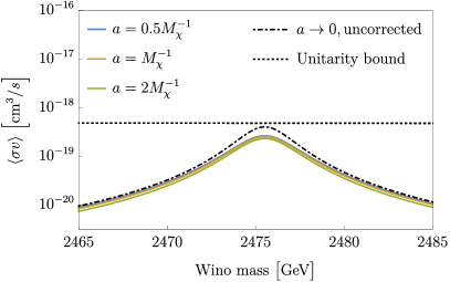
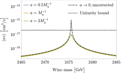
Figure 10: Colored lines show the Sommerfeld-enhanced annihilation cross section for wino dark matter, using the corrected expression derived in this work, for different choices of the matching radius $a$. The dot-dashed black line shows the result of computing the uncorrected Sommerfeld-enhanced annihilation cross section. The relative velocity between DM particles is taken to be $v=10^{-4}$ (left) or $v=10^{-6}$ (right). The dotted black line indicates the unitarity bound on the annihilation cross section.

At $v_{\text{rel}}=10^{-4}$, the uncorrected cross section approaches the unitarity bound and the correction induces a non-negligible suppression. This suppression is more pronounced for $v_{\text{rel}}=10^{-6}$, where the uncorrected result significantly exceeds the unitarity bound on resonance. The corrected results all respect the unitarity bound, as we expect by construction. Note that in the case of $v_{\text{rel}}=10^{-6}$, the corrected cross section does not come close to saturating the unitarity limit; the effect of the correction is not simply to provide an upper limit on the cross section at a given momentum.

We demonstrate the velocity dependence of the corrected and uncorrected cross section near the resonance in Fig. 11, for two different masses corresponding to the cases where the uncorrected cross section exceeds the unitarity bound, in one case only slightly and for a small range of momenta, and in the other case by a large factor (with the second case being closer to the resonance peak). We observe that as $v_{\text{rel}}$ is decreased, in both cases the corrected cross section saturates at a roughly $v_{\text{rel}}$-independent value soon after approaching the unitarity bound. In the first case, this induces only a modest shift in the saturation velocity and saturated cross section relative to the uncorrected calculation, but in the second case, this leads to earlier saturation and a much lower cross section (again relative to the uncorrected results).

The low-velocity saturated cross section near the resonance can be compared to the results of the zero-range effective field theory of Ref. Braaten:2017dwq , which provides a unitarized result for the inclusive wino annihilation cross section that is valid in proximity to the resonance. That work found that the resonance peak was at 2.39 TeV, offset from ours by a few percent, so we should not expect agreement in the cross sections better than this level; we note that the resonance position is sensitive to the exact choice of electroweak parameters and to higher-order corrections to the potential (see App. E). That work finds that at the resonance, $\gamma_{0}=9.59\times 10^{-4}i\times 28.5\text{GeV}$, corresponding to a cross section in the low-velocity limit of $\sigma_{\text{ann}}v_{\text{rel}}=16\pi/(M_{\chi}\text{Im}\gamma_{0})=0.769\text{GeV}^{-2}=8.98\times 10^{-18}$ cm³/s, which is very similar to the result shown in Fig. 11 ($\sigma_{\text{ann}}v_{\text{rel}}=1.02\times 10^{-17}$ cm³/s for the nearest-resonance mass and lowest velocity we tested). Our methods are quite different so this correspondence is encouraging.

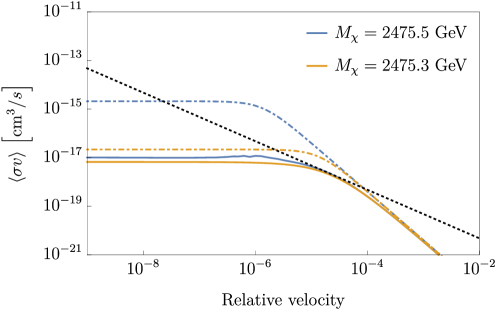
Figure 11: Colored lines show the Sommerfeld-enhanced annihilation cross section for wino dark matter, using the corrected expression derived in this work and taking $a=1/M_{\chi}$, for different choices of the wino mass in proximity to the first resonance. For each mass, the solid line shows the full result and the dot-dashed line shows the uncorrected Sommerfeld-enhanced result. The black dotted line shows the unitarity bound at the mass corresponding to the center of the resonance (the mass variation between the different lines in this figure changes the unitarity bound at the sub-percent level).

5 Conclusions

We have derived a general expression for the regulated Sommerfeld enhancement, valid for arbitrary partial waves and where multiple states are coupled by the long-range potential. We assume a hierarchy between the momentum scale associated with the long-range potential (parametrically $\alpha M_{\chi}$) and the momentum scale associated with the short-range physics (parametrically $M_{\chi}$ for annihilation), and further assume that the $S$-matrix element associated with the long-range potential $S_{0,\ell}$ satisfies $S_{0,\ell}^{\dagger}S_{0,\ell}=1$. Under these assumptions, we have demonstrated that the full cross section, which manifestly preserves unitarity, can be written in terms of the conventional Sommerfeld enhancement and a corrected scattering amplitude $\kappa_{\ell}$, for any partial wave $\ell$ and for arbitrary numbers of states coupled by the potential. The corrected amplitude $\kappa_{\ell}$ can be constructed in general from the short-distance amplitude $f_{s,\ell}$ and two additional factors obtained by solving the Schrödinger equation with the long-range potential, and we have explored its generic properties for the case where only a single two-particle state is involved.

We have provided expressions for the corrected $S$-matrix and cross section valid when any number of the states are kinematically allowed at asymptotically large distances, as well as simplified expressions valid for the one-state case. We have confirmed we can reproduce earlier expressions in the literature for the leading-order multi-state Sommerfeld enhancement for arbitrary $\ell$, as well as the manifestly unitarity-preserving cross section for the $s$-wave single-state case, and the near-resonance behavior previously studied using zero range effective field theory in the case of the wino. Our expressions nominally depend on the matching radius, but we have shown (analytically in the single-state case and numerically in a multi-state example) that the leading dependence on the matching radius can be absorbed/canceled, and the residual dependence is small. We expect that a more complete effective field theory treatment, including higher-order corrections to both the potential and the short-range physics, would remove the residual dependence on the matching radius.

One point of interest is that we have found that even when the uncorrected cross section is well below the unitarity bound at a given velocity, there can be significant corrections to the standard expression in cases where the uncorrected cross section at higher velocities exceeds the unitarity bound. Our method helps clarify the origin of these corrections, which can be cast as modifications to the effective short-range matrix element from the long-range potential.

Appendix A Analytic properties of $F_{\ell}$ and $G_{\ell}$

In this appendix, we discuss the analytic properties of the $F_{\ell}$ and $G_{\ell}$ basis solutions defined in Sec. 2.2, following the discussion of e.g., Ref. teichmann1951interpretation . We assume the most singular term of the potential at the origin is $1/r$ and the potential can be expanded as a series in $r$:

$$2\mu V(r)=\sum_{k=-1}^{\infty}v_{k}r^{k}.$$ (170)

A.1 Regular solution : $F_{\ell}$

The regular solution $F_{\ell}$ can be expanded as a power series in $r$:

$$F_{\ell}(r)=C_{\ell}p^{\ell+1}\sum_{k=\ell+1}^{\infty}f_{\ell,k}r^{k}.$$ (171)

In order to be consistent with the boundary condition of Eq. 18, the coefficient of the $r^{\ell+1}$ term is determined to be

$$f_{\ell,\ell+1} =\frac{1}{(2\ell+1)!!}.$$ (172)

The Schrödinger equation Eq. 15 around $r=0$ tells us the recurrence relation for $f_{\ell,k}$ with $k\geq\ell+2$:

$$-(2\ell+2)f_{\ell,\ell+2}+v_{-1}f_{\ell,\ell+1}=0,$$ (173)

$$[-k(k-1)+\ell(\ell+1)]f_{\ell,k}+\left(\sum_{m=-1}^{k-\ell-3}v_{m}f_{\ell,k-2-m}\right)-p^{2}f_{\ell,k-2}=0\qquad(k\geq\ell+3).$$ (174)

We can determine $f_{\ell,k}$ by applying this recurrence relation repeatedly starting from small $k$, and see that all of the $f_{\ell,k}$ coefficients are analytic functions of $p^{2}$.

A.2 Irregular solution : $G_{\ell}$

On the other hand, the irregular solution $G_{\ell}(r)$ can be expanded as

$$G_{\ell}(r) =\frac{1}{C_{\ell}p^{\ell}}\left[\sum_{k=-\ell}^{\infty}g_{\ell,k}r^{k}+x_{\ell}\log\frac{r}{r_{0}}\times\frac{1}{C_{\ell}p^{\ell+1}}F_{\ell}(r)\right]$$

$$=\frac{1}{C_{\ell}p^{\ell}}\left[\sum_{k=-\ell}^{\infty}g_{\ell,k}r^{k}+x_{\ell}\sum_{k=\ell+1}^{\infty}f_{\ell,k}r^{k}\log\frac{r}{r_{0}}\right].$$ (175)

Here $r_{0}$ is introduced to make the argument of the logarithm dimensionless. Shifting $r_{0}$ can be absorbed by a redefinition of $g_{\ell,\ell+1},~{}g_{\ell,\ell+2},~{}\cdots$. In order to be consistent with the boundary condition of Eq. 18, the coefficient of $r^{-\ell}$ term can be determined as

$$g_{\ell,-\ell} =(2\ell-1)!!.$$ (176)

The Schrödinger equation Eq. 15 around $r=0$ tells us the recurrence relation for $g_{\ell,k}$ with $k\geq\ell+2$. For $\ell=0$,

$$v_{-1}g_{0,0}+x_{0}f_{0,1}=0,$$ (177)

$$-k(k-1)g_{0,k}+\left(\sum_{m=-1}^{k-2}v_{m}g_{0,k-2-m}\right)-p^{2}g_{0,k-2}+x_{0}kf_{0,k}=0\qquad(k\geq 2),$$ (178)

For $\ell\geq 1$,

$$2\ell g_{\ell,-\ell+1}+v_{-1}g_{\ell,-\ell}=0,$$ (179)

$$[-k(k-1)+\ell(\ell+1)]g_{\ell,k}+\left(\sum_{m=-1}^{k-2+\ell}v_{m}g_{\ell,k-2-m}\right)-p^{2}g_{\ell,k-2}=0\qquad(-\ell+2\leq k\leq\ell),$$ (180)

$$\left(\sum_{m=-1}^{2\ell-1}v_{m}g_{\ell,\ell-1-m}\right)-p^{2}g_{\ell,\ell-1}+x_{\ell}(\ell+1)f_{\ell,\ell+1}=0,$$ (181)

$$[-k(k-1)+\ell(\ell+1)]g_{\ell,k}+\left(\sum_{m=-1}^{k-2+\ell}v_{m}g_{\ell,k-2-m}\right)-p^{2}g_{\ell,k-2}+x_{\ell}kf_{\ell,k}=0\qquad(k\geq\ell+2).$$ (182)

We can determine many of the coefficients by applying the recurrence relations in the following order: $g_{\ell,-\ell},g_{\ell,-\ell+1},\ldots,g_{\ell,\ell},x_{\ell},g_{\ell,\ell+2},g_{\ell,\ell+3},\ldots$. On the other hand, we cannot determine $g_{\ell,\ell+1}$ from this procedure. $g_{\ell,\ell+1}$ can be determined by imposing the boundary condition on $G_{\ell}$ at $r\to\infty$ given in Eq. 17.

A.3 Momentum dependence of $x_{\ell}(p)$

Let us discuss the momentum dependence of $x_{\ell}(p)$ in the expansion of $G_{\ell}(r)$ given in Eq. 175. This property is important for the renormalization discussion given in Sec. 2.4.2.

For the $s$-wave case ($\ell=0$), Eqs. 172, 176, 177 tell us that

$$x_{0}=-v_{-1}.$$ (183)

Thus, we can see $x_{0}$ is constant ($p$-independent) for the $s$-wave case. On the other hand, $x_{\ell}$ with $\ell\geq 1$ can be determined from Eqs. 172, 181 as:

$$x_{\ell}=-\frac{(2\ell+1)!!}{\ell(\ell+1)}\left[\left(\sum_{m=-1}^{2\ell-1}v_{m}g_{\ell,\ell-1-m}\right)-p^{2}g_{\ell,\ell-1}\right].$$ (184)

Thus, for higher partial waves ($\ell\geq 1$) $x_{\ell}$ is momentum-dependent except in special cases.

As one example of such a special case, let us discuss a potential $V(r)$ which does not contain any odd powers of $r$, i.e.,

$$v_{-1}=v_{1}=v_{3}=\cdots=0.$$ (185)

This is the case when the potential $V(r)$ is an analytic function of $x$, $y$, and $z$ around the origin. In this case, by using the recurrence relations, we can show that

$$g_{\ell,-\ell+1}=g_{\ell,-\ell+3}=g_{\ell,-\ell+5}=\cdots=0.$$ (186)

Then, we obtain

$$x_{\ell}=0.$$ (187)

Appendix B Variable phase method for irregular solutions

It can be helpful to directly numerically compute the solutions to the multi-state Schrödinger equation with perturbed short-distance boundary conditions (corresponding to irregular solutions of the Schrödinger equation with the usual long-range potential). For such cases, we can adapt the variable phase method proposed in Ref. PhysRevC.84.064308 as recast in Refs. Beneke:2014gja ; Asadi:2016ybp . Following the notation of Ref. Asadi:2016ybp , we can decompose a reduced radial wavefunction $u(r)$ as:

$$u_{n}(r)=\alpha_{n}(r)f_{n}(r)-\beta_{n}(r)g_{n}(r),$$ (188)

where $n$ indexes the component and there is no summation over $n$ on the right-hand side, and as previously (e.g. Eq. 12), $f_{n}(r)=s_{\ell}(p_{n}r)/\sqrt{p_{n}}$ and $g_{n}(r)=\left[c_{\ell}(p_{n}r)+is_{\ell}(p_{n}r)\right]/\sqrt{p_{n}}$. In particular, at large $r$, $g_{n}(r)\propto e^{ip_{n}r}$, the purely outgoing mode, and $g_{n}(r)$ is irregular at the origin, while $f_{n}(r)$ is regular. We may add a second index to describe an ensemble of solutions, as in the discussion below Eq. 131. For the Schrödinger equation with no potential, and an incoming wave in the $i$th state, $u_{ni}(r)=\delta_{ni}f_{n}(r)$ and $u_{ni}(r)=\delta_{ni}g_{n}(r)$ are independent solutions for each choice of $i$, and so their Wronskian is constant: by considering the large-$r$ regime, it then follows straightforwardly that $f_{n}^{\prime}g_{n}-f_{n}g_{n}^{\prime}=1$ for each choice of $n$ (this can also be checked directly).

As in Ref. Asadi:2016ybp , to account for the extra degrees of freedom induced by solving for two functions rather than one, we will impose the additional condition:

$$\alpha_{a}^{\prime}(r)f_{a}(r)-\beta_{a}^{\prime}(r)g_{a}(r)=0,$$ (189)

for each individual choice of $n$ and $i$.

The setup in Ref. Asadi:2016ybp is appropriate for determining the regular solution. Suppose we are instead interested in the irregular outgoing solutions, e.g. those labeled $\tilde{w}_{ni}(r)$ in Sec. 3.2, with non-zero $\beta_{n}(r)$ at small $r$, and $\alpha_{n}(r)\rightarrow 0$ at large $r$. Let us write $\alpha_{a}(r)=O_{ab}(r)\beta_{b}(r)$; we will solve for $O_{ab}(r)$ and $\beta_{a}(r)$.

These functions can be obtained by solving the first-order differential equations:

$$O_{ab}^{\prime}(r) =\sum_{c,d}(g_{a}\delta_{ac}-O_{ac}f_{c})\hat{U}_{cd}(g_{b}\delta_{bd}-f_{d}O_{db})$$

$$\beta_{a}^{\prime} =\sum_{b,c}f_{a}\hat{U}_{ac}(g_{b}\delta_{cb}-f_{c}O_{cb})\beta_{b},$$ (190)

where $\hat{U}_{ac}$ can be read off from the potential matrix for the multi-state system.

To check this, note that if these equations are satisfied, then we obtain:

$$\alpha_{a}^{\prime}(r)f_{a}(r)-\beta_{a}^{\prime}(r)g_{a}(r)$$ (191)

$$=O_{ab}^{\prime}\beta_{b}f_{a}+O_{ab}\beta_{b}^{\prime}f_{a}-\beta_{a}^{\prime}g_{a}$$

$$=(g_{a}\delta_{ac}-O_{ac}f_{c})\hat{U}_{cd}(g_{b}\delta_{bd}-f_{d}O_{db})\beta_{b}f_{a}+f_{a}O_{ab}f_{b}\hat{U}_{bc}(g_{d}\delta_{cd}-f_{c}O_{cd})\beta_{d}$$

$$-(f_{a}\hat{U}_{ac}g_{c}\beta_{c}-f_{a}\hat{U}_{ac}f_{c}O_{cb}\beta_{b})g_{a}$$

$$=g_{a}g_{b}\hat{U}_{ab}\beta_{b}f_{a}+O_{ac}f_{c}\hat{U}_{cd}f_{d}O_{db}\beta_{b}f_{a}-g_{a}\hat{U}_{ad}f_{d}O_{db}f_{a}\beta_{b}-O_{ac}f_{c}\hat{U}_{cb}g_{b}\beta_{b}f_{a}$$

$$+f_{a}O_{ab}f_{b}\hat{U}_{bc}g_{c}\beta_{c}-f_{a}O_{ab}f_{b}\hat{U}_{bc}f_{c}O_{cd}\beta_{d}-(f_{a}\hat{U}_{ac}g_{c}\beta_{c}-f_{a}\hat{U}_{ac}f_{c}O_{cb}\beta_{b})g_{a}$$

$$=0,$$ (192)

as required. Furthermore,

$$u_{n}^{\prime\prime}(r) =\left[\alpha_{n}(r)f_{n}^{\prime}(r)-\beta_{n}(r)g^{\prime}_{n}(r)\right]^{\prime}$$

$$=\alpha^{\prime}_{n}(r)f_{n}^{\prime}(r)-\beta^{\prime}_{n}(r)g^{\prime}_{n}(r)+\alpha_{n}(r)f_{n}^{\prime\prime}(r)-\beta_{n}(r)g^{\prime\prime}_{n}(r)$$

$$=\beta^{\prime}_{n}(r)g_{n}(r)f_{n}^{\prime}(r)/f_{n}(r)-\beta^{\prime}_{n}(r)g^{\prime}_{n}(r)+\alpha_{n}(r)f_{n}^{\prime\prime}(r)-\beta_{n}(r)g^{\prime\prime}_{n}(r)$$

$$=\frac{\beta^{\prime}_{n}(r)}{f_{n}(r)}\left[g_{n}(r)f_{n}^{\prime}(r)-g^{\prime}_{n}(r)f_{n}(r)\right]+\alpha_{n}(r)f_{n}^{\prime\prime}(r)-\beta_{n}(r)g^{\prime\prime}_{n}(r)$$

$$=\hat{U}_{nc}(g_{b}(r)\delta_{cb}-f_{c}O_{cb}(r))\beta_{b}(r)+\alpha_{n}(r)f_{n}^{\prime\prime}(r)-\beta_{n}(r)g^{\prime\prime}_{n}(r)$$

$$=-\hat{U}_{nb}u_{b}(r)+\alpha_{n}(r)f_{n}^{\prime\prime}(r)-\beta_{n}(r)g^{\prime\prime}_{n}(r)$$ (193)

Since $f_{n}$ and $g_{n}$ are solutions to the Schrödinger equation with no potential and momentum $p_{n}$, we can write $f_{n}^{\prime\prime}(r)=(\ell(\ell+1)/r^{2}-p_{n}^{2})f_{n}(r)$, $g_{n}^{\prime\prime}(r)=(\ell(\ell+1)/r^{2}-p_{n}^{2})g_{n}(r)$, and thus we obtain:

$$u_{n}^{\prime\prime}(r) =-\hat{U}_{nb}u_{b}(r)+(\ell(\ell+1)/r^{2}-p_{n}^{2})\left[\alpha_{n}(r)f_{n}(r)-\beta_{n}(r)g_{n}(r)\right]$$

$$=\left[\frac{\ell(\ell+1)}{r^{2}}\delta_{nb}-p_{n}^{2}\delta_{nb}-\hat{U}_{nb}\right]u_{b}(r)$$ (194)

By comparison to Eq. 102, we see that we should identify $\hat{U}=-2\mu\hat{V}_{\text{long}}$.

We will often be interested in purely outgoing solutions, in which case we will require $O_{ab}\rightarrow 0$ at large $r$. Note that the equation for $O_{ab}$ is nonlinear and in particular $O_{ab}=0$ is not a valid solution in the presence of a non-zero long-range potential, so imposing this boundary condition will not automatically lead to a trivial solution. Our first step in studying a purely outgoing solution is thus to solve the first line of Eq. 190 for $O_{ab}(r)$ with the boundary condition $O_{ab}(r\rightarrow\infty)=0$.

In particular, consider the $\tilde{w}_{\ell}(r)$ solutions introduced in Eq. 109, with components $\tilde{w}_{ni}$; here $n$ indexes the component and $i$ describes the small-$r$ boundary condition. As shown in Eq. 132, the small-$r$ boundary conditions for these solutions can be written in matrix form as $\beta_{\tilde{w}_{\ell}}(0)=\beta_{\tilde{G}_{\ell}}(0)+i\beta_{\tilde{F}_{\ell}}(0)=-\tilde{P}^{2\ell+1}$. This fully specifies the boundary conditions needed to solve for $\tilde{w}_{\ell}(r)$.

In order to compute the corrected cross sections in this work, for general choices of the convention for $V_{\text{long}}(r)$ at $r<a$, we need to compute the $\alpha_{b,\ell}(0)$ matrices derived from regular solutions to the Schrödinger equation, the standard uncorrected Sommerfeld enhancement $\Sigma_{0,\ell}$, and the matrix $\alpha_{\tilde{G}_{\ell}}(a)$. For regular solutions we employ the method described in Appendix A of Ref. Asadi:2016ybp . In the notation of that work, we solve for $\tilde{\alpha}_{ni}(r)\equiv\alpha_{ni}(r)/g_{n}(r)$. The prescription defined in the text for $\alpha_{b,\ell}(0)$ is to set boundary conditions of $\alpha_{b,\ell}(a)=\tilde{P}$, and then read off $\alpha_{b,\ell}(0)$ for a regular solution. This amounts to setting boundary conditions on $\tilde{\alpha}_{ni}(a)\equiv\delta_{ni}\sqrt{p_{n}}/g_{n}(a)$, and then extracting $\tilde{\alpha}_{ni}(0)g_{n}(0)$.

The methods of Appendix A of Ref. Asadi:2016ybp can likewise be applied to directly solve for the regular solution $w_{\ell}(r)$. Once (the $\alpha$ functions for) both $\tilde{w}_{\ell}(r)$ and $w_{\ell}(r)$ are in hand, the matrix $\alpha_{\tilde{G}_{\ell}}(a)$ satisfies:

$$\alpha_{\tilde{w}_{\ell}}(r) =\alpha_{\tilde{G}_{\ell}}(r)+i\alpha_{w_{\ell}}(r)P^{-1}\bar{Q}^{\dagger}_{\ell}$$

$$\Rightarrow\alpha_{\tilde{G}_{\ell}}(a) =\alpha_{\tilde{w}_{\ell}}(a)-i\alpha_{w_{\ell}}(a)\Sigma_{0,\ell}^{\dagger}(\tilde{P}^{\dagger})^{2\ell}$$ (195)

The standard Sommerfeld factor $\Sigma_{0,\ell}$ can be extracted from the regular solution $w_{\ell}(r)$, computed as in Ref. Asadi:2016ybp , or from the irregular solution $\tilde{w}_{\ell}$ (which is equivalent to the widely-used approach of extracting the Sommerfeld enhancement from the behavior of the irregular solution at large $r$), by solving the second line of Eq. 190 for $\beta_{\tilde{w}_{\ell}}(r)$. We observe that $-\lim_{r\rightarrow\infty}(\beta_{\tilde{w}_{\ell}}(r))_{ni}/\sqrt{p_{n}}$ is the coefficient of $c_{\ell}(p_{n}r)+is_{\ell}(p_{n}r)$ for the $n$th component, and consequently $\lim_{r\rightarrow\infty}(\beta_{\tilde{w}_{\ell}}(r))_{nj}=-\sqrt{p_{n}}p_{j}f_{1,nj}$ (Eq. 112). Since $\Sigma_{0,\ell}=\tilde{P}^{2}Q_{\ell}P^{-2}$ and $f_{1,ij}=(p_{j}^{\ell}/p_{i})Q_{ji}$ for $i\leq M$ (as derived below Eq. 116), we have $-\lim_{r\rightarrow\infty}(\beta_{\tilde{w}_{\ell}}(r))_{nj}=(p_{j}^{\ell+1}/\sqrt{p_{n}})Q_{jn}$, and $\Sigma_{0,ij}=p_{i}Q_{ij}/p_{j}$, so finally we obtain:

$$\Sigma_{0,ij}=-\frac{1}{p_{i}^{\ell}\sqrt{p_{j}}}\lim_{r\rightarrow\infty}(\beta_{\tilde{w}_{\ell}}(r))_{ji},\quad\Sigma_{0,\ell}=-\lim_{r\rightarrow\infty}\left(P^{-1}\beta_{\tilde{w}_{\ell}}(r)\tilde{P}^{-2\ell}\right)^{T},$$ (196)

where in the final matrix expression we truncate $\beta_{\tilde{w}_{\ell}}(r)$ to $M\times N$, i.e. we only need to read off the components for the states that are kinematically accessible.

We can use this construction to show that $O_{ab}(r)$ is always symmetric, provided the long-range potential matrix is symmetric and the boundary condition on $O_{ab}$ is symmetric. Let us consider the evolution equations for $O_{ab}(r)$ and $O_{ba}(r)$. We have:

$$O_{ab}^{\prime}(r) =\sum_{c,d}(g_{a}\delta_{ac}-O_{ac}f_{c})\hat{U}_{cd}(g_{b}\delta_{bd}-f_{d}O_{db})$$

$$O_{ba}^{\prime}(r) =\sum_{c,d}(g_{b}\delta_{bc}-O_{bc}f_{c})\hat{U}_{cd}(g_{a}\delta_{ad}-f_{d}O_{da}).$$ (197)

Relabeling dummy variables ($c\leftrightarrow d$) in the second equation, and using $\hat{U}_{cd}=\hat{U}_{dc}$ by symmetry of the potential, we have:

$$O_{ba}^{\prime}(r) =\sum_{c,d}(g_{a}\delta_{ac}-O_{ca}f_{c})\hat{U}_{cd}(g_{b}\delta_{bd}-f_{d}O_{bd}).$$ (198)

We observe that if $O=O^{T}$ at a point (so $O_{ca}=O_{ac}$ and $O_{bd}=O_{db}$), then the derivatives of $O_{ba}$ and $O_{ab}$ will also coincide at that point, and thus the evolution equation will preserve the relation $O=O^{T}$. Thus provided we have a symmetric initial/boundary condition, $O$ will remain symmetric for all $r$.

Now for $r\rightarrow 0$, for the $\tilde{w}_{ni}$ solutions, $p_{a}^{\ell+1/2}\alpha_{ai}=p_{a}^{\ell+1/2}O_{ab}\beta_{bi}\rightarrow-O_{ab}p_{a}^{\ell+1/2}p_{b}^{\ell+1/2}\delta_{bi}=-O_{ai}p_{a}^{\ell+1/2}p_{i}^{\ell+1/2}$, which is invariant under $a\leftrightarrow i$. Thus $\tilde{P}^{2\ell+1}\alpha$ is symmetric for the $\tilde{G}_{\ell}(r)$ and $\tilde{F}_{\ell}(r)$ solutions (corresponding to the real and imaginary parts of $\tilde{w}_{\ell}$).

Finally, we note that given two solutions $u$ and $v$ with corresponding $\alpha$ and $\beta$ functions $\alpha_{u},\alpha_{v},\beta_{u}$ and $\beta_{v}$, we can compute the Wronskian as (again assuming a real symmetric potential):

$$(u^{\prime})^{T}v-u^{T}v^{\prime} =\sum_{a}\left[(\alpha_{ua}(r)f_{a}^{\prime}(r)-\beta_{ua}(r)g_{a}^{\prime}(r))(\alpha_{va}(r)f_{a}(r)-\beta_{va}(r)g_{a}(r))\right.$$

$$\left.-(\alpha_{ua}(r)f_{a}(r)-\beta_{ua}(r)g_{a}(r))(\alpha_{va}(r)f_{a}^{\prime}(r)-\beta_{va}(r)g^{\prime}_{a}(r))\right]$$

$$=\sum_{a}(\alpha_{ua}(r)\beta_{va}(r)-\beta_{ua}(r)\alpha_{va}(r))(-f_{a}^{\prime}(r)g_{a}(r)+f_{a}(r)g^{\prime}_{a}(r)),$$

$$=-(\alpha_{u}^{T}\beta_{v}-\beta_{u}^{T}\alpha_{v}).$$ (199)

Appendix C Calculating the short-distance amplitude $f_{s,\ell}$

C.1 Normalization convention and optical theorem

Since the $f_{s,\ell}$ contribution to $\kappa_{\ell}$ (see Eq. 141) describes only short-distance physics, it can be calculated using the Born approximation or perturbative QFT (assuming a weakly-coupled theory). For contributions that can be captured by a non-relativistic potential, the Born approximation will often be the simplest approach, but for more general interactions, a field-theoretic approach may be necessary. For convenience, let us review the translation from $f_{s,\ell}$ to the matrix element $i\mathcal{M}$ of QFT; we here follow the notation and conventions of Ref. Peskin:1995ev .

The first Born approximation for scattering of two distinguishable particles in quantum mechanics can be written in the form:

$$f_{s}\approx-\frac{2\mu}{4\pi}\int d^{3}\vec{r}e^{i\vec{q}\cdot\vec{r}}V(\vec{r})=-\frac{\mu}{2\pi}\tilde{V}(\vec{q}),$$ (200)

where $\tilde{V}(\vec{q})$ denotes the Fourier transform of the potential, and $\mu$ is the reduced mass. Working at the same (leading) order, Ref. Peskin:1995ev relates the potential to the (relativistically normalized) matrix element via $\frac{1}{(4\mu)^{2}}(i\mathcal{M})=-i\tilde{V}(\vec{q})$, where the factors of $4\mu$ arise from the difference between relativistic and non-relativistic normalizations of the states (and we assume here $2\rightarrow 2$ scattering where all the particle masses are equal at leading order). Thus we identify $f_{s}=\frac{1}{32\pi\mu}\mathcal{M}$ for distinguishable particles (at least at leading order). For $2\rightarrow 2$ scattering, we can extract the individual partial waves by tracking the dependence of $\mathcal{M}$ on the angle $\theta$ between the incoming and outgoing momenta, and computing:

$$(f_{s,\ell})_{fi} =\frac{1}{64\pi\mu}\int^{1}_{-1}d\cos\theta P_{\ell}(\cos\theta)\mathcal{M}(i\rightarrow f)(\theta).$$ (201)

Where identical particles are involved, this relationship should be corrected to $f_{s}=\frac{1}{32\pi\mu}\mathcal{M}/\sqrt{2^{\delta_{a}}2^{\delta_{b}}}$, where $a$ and $b$ label the initial and final states respectively, and $\delta_{X}=1$ for identical particles and 0 for distinguishable particles; this corresponds to working with the “rescaled partial-wave amplitudes” discussed in Ref. Flores:2024sfy . In the multi-state case, this agrees with the standard rescaling factors for the “method-2” annihilation matrix discussed in Ref. Beneke:2014gja . Here $f_{s}$ remains the scattering amplitude calculated via quantum mechanics for the case of distinguishable particles (which is the quantity we generally work with in the main text), but $\mathcal{M}$ is the QFT amplitude calculated using all standard rules.

In the case where both initial and final states contain identical particles, the factor of 2 (relative to the quantum mechanics calculation with distinguishable particles) is due to the inclusion of “crossed ladder” diagrams (as well as ladder diagrams) in the QFT amplitude. In the case where only one of the states contains distinguishable particles, the factor of $\sqrt{2}$ in the QFT amplitude can be viewed as the combined effect of including the crossed diagrams (factor of 2), and the fact that our “method-2” potential for the quantum mechanics calculation (e.g. Eq. 163 already includes a factor of $\sqrt{2}$ for this transition, relative to what one would expect from the tree-level diagram with all distinguishable particles (factor of $1/\sqrt{2}$). In the case where both incoming and outgoing states consist of distinguishable particles, there is no extra rescaling and the standard conversion factor above applies.

As usual, for the bare annihilation rate, we can further simplify the calculation using the optical theorem. As per Ref. Flores:2024sfy , the optical theorem takes its usual simple form when applied to the rescaled amplitudes that account for the identical-particle factors given above, so we will assume below that the matrix elements $\mathcal{M}$ have been rescaled as necessary (and so can be converted to our quantum-mechanical $f_{s}$ amplitudes for distinguishable particles by the conversion factor $32\pi\mu$).

There is an additional subtlety with regard to the case with imaginary momenta, where for $f_{s,\ell}$ we need the full $N\times N$ matrix, not just its $M\times M$ truncation (physically, this can be understood as the potential providing energy to excite states which would be kinematically forbidden in its absence). It is not immediately clear how to define the QFT matrix element in this case. If we can factor out the momentum dependence of the amplitudes, so that they are characterized in terms of momentum-independent coefficients, then we can match these momentum-independent coefficients in the regime where all the states are kinematically accessible; we can also use the optical theorem to compute these coefficients. Then we can obtain $f_{s,\ell}$ at lower momentum by restoring the (possibly complex) momentum factors.

The standard optical theorem result (for real momenta) is:

$$-i\left[\mathcal{M}(a\rightarrow b)-\mathcal{M}^{*}(b\rightarrow a)\right]=\sum_{X}\int d\Pi_{X}\mathcal{M}^{*}(b\rightarrow X)\mathcal{M}(a\rightarrow X).$$ (202)

Here $a$ and $b$ denote the non-relativistic initial and final states coupled by the potential, and $X$ denotes all possible intermediate states. We can apply this result to each partial wave separately, by replacing $\mathcal{M}(a\rightarrow X)=\sum_{\ell}P_{\ell}(\cos\theta)(2\ell+1)\mathcal{M}_{\ell}(a\rightarrow X)$; the double sum on the RHS will collapse to a single sum upon integration of the $P_{\ell}(\cos\theta)$ terms over the final-state phase space.

Now suppose that for a given partial-wave cross section, evaluated at real momenta, we have $\mathcal{M}_{\ell}(a\rightarrow b)=(p_{a}p_{b}/\mu^{2})^{\ell}\hat{\mathcal{M}}_{\ell}(a\rightarrow b)$ where the hatted amplitude is independent of the external momenta. Similarly, suppose we can write $\mathcal{M}_{\ell}(a\rightarrow X)=(p_{a}p_{X}/\mu^{2})^{\ell}\hat{\mathcal{M}}_{\ell}(a\rightarrow X)$, where $p_{X}$ is defined as usual if $X$ is one of the non-relativistic two-particle states coupled by the potential, and otherwise can be left unspecified (or can be e.g. defined to be equal to $\mu$; we will see that this factor does not matter). Here we want $\hat{\mathcal{M}}_{\ell}(a\rightarrow X)$ to be independent of any external momenta associated with the non-relativistic two-particle states coupled by the potential.

Then in the optical theorem, evaluated at real $p_{a}$, $p_{b}$, we can cancel out the momentum factors associated with the initial/final states and obtain:

$$-i\left[\hat{\mathcal{M}}(a\rightarrow b)-\hat{\mathcal{M}}^{*}(b\rightarrow a)\right]=\sum_{X}\int d\Pi_{X}|p_{X}/\mu|^{2}\hat{\mathcal{M}}^{*}(b\rightarrow X)\hat{\mathcal{M}}(a\rightarrow X).$$ (203)

If these equations continue to hold when we extend to the case of imaginary momenta, we can write:

$$-i(p_{b}^{*}p_{a}/\mu^{2})^{\ell}\left[\hat{\mathcal{M}}(a\rightarrow b)-\hat{\mathcal{M}}^{*}(b\rightarrow a)\right]=(p_{b}^{*}p_{a}/\mu^{2})^{\ell}\sum_{X}\int d\Pi_{X}|p_{X}/\mu|^{2}\hat{\mathcal{M}}^{*}(b\rightarrow X)\hat{\mathcal{M}}(a\rightarrow X)$$

$$\Rightarrow -i\left[(p_{b}^{*}/p_{b})^{\ell}\mathcal{M}(a\rightarrow b)-(p_{a}/p_{a}^{*})^{\ell}\mathcal{M}^{*}(b\rightarrow a)\right]=\sum_{X}\int d\Pi_{X}\mathcal{M}^{*}(b\rightarrow X)\mathcal{M}(a\rightarrow X).$$ (204)

This explains why our expression for the cross section (e.g. in Eq. 3.5) is most simply written in terms of $\bar{f}_{s,\ell}$ rather than $f_{s,\ell}$; if, following the conventions above, we identify $(f_{s,\ell})_{ba}=\frac{1}{32\pi\mu}\mathcal{M}_{\ell}(a\rightarrow b)=(p_{a}p_{b}/\mu^{2})^{\ell}\hat{\mathcal{M}}_{\ell}(a\rightarrow b)$, then $(\bar{f}_{s,\ell})_{ba}=\frac{1}{32\pi\mu}\mathcal{M}_{\ell}(a\rightarrow b)(p_{b}^{*}/p_{b})^{\ell}$, and we can write from the optical theorem above:

$$\frac{2\pi i}{\mu}(\bar{f}_{s,\ell}^{\dagger}-\bar{f}_{s,\ell})_{ba} =\frac{1}{(4\mu)^{2}}\sum_{X}\int d\Pi_{X}\mathcal{M}_{\ell}^{*}(b\rightarrow X)\mathcal{M}_{\ell}(a\rightarrow X).$$ (205)

In this case, the RHS includes all possible final states, including the kinematically allowed states coupled by the potential; to obtain the inclusive annihilation cross section, we must subtract this scattering term. It can easily be seen that this subtraction is implemented by the $\bar{f}_{s,\ell}^{\dagger}(\bar{Z}^{\dagger}-\bar{Z})\bar{f}_{s,\ell}$ term in Eq. 3.5 (which as discussed in the main text is independent of the long-range potential, and depends only on the scattering amplitude into kinematically allowed states). Thus we can replace $\bar{f}_{s,\ell}^{\dagger}-\bar{f}_{s,\ell}\rightarrow\bar{f}_{s,\ell}^{\dagger}-\bar{f}_{s,\ell}+\bar{f}_{s,\ell}^{\dagger}(\bar{Z}^{\dagger}-\bar{Z})\bar{f}_{s,\ell}$ on the LHS of Eq. 205 if we understand the sum on the RHS to include only final states for annihilation, not scattering. For the diagonal terms ($a=b$), we recognize the familiar expression for the cross section on the RHS (in the absence of Sommerfeld enhancement, and up to the $c_{i}$ factor for identical particles).

C.2 Results for the wino example

We can now go ahead and use existing results for the wino to write out the components of the bare annihilation matrix; for simplicity, let us write $\bar{\Gamma}_{\ell}\equiv\bar{f}_{s,\ell}^{\dagger}-\bar{f}_{s,\ell}+\bar{f}_{s,\ell}^{\dagger}(\bar{Z}^{\dagger}-\bar{Z})\bar{f}_{s,\ell}$. Refs. Hellmann:2013jxa ; Beneke:2014gja provide Wilson coefficients for the pure wino that encode $\sum_{X}\int d\Pi_{X}\hat{\mathcal{M}}_{\ell}^{*}(b\rightarrow X)\hat{\mathcal{M}}_{\ell}(a\rightarrow X)$, as also discussed in Ref. Asadi:2016ybp . As discussed above, we are using the “method-2” basis of Ref. Beneke:2014gja to define the two-particle states, and so must rescale the elements of the annihilation matrix that involve identical-particle states. Specifically, for $\ell=0$ we can replace $\frac{1}{(4\mu)^{2}}\left[\sum_{X}\int d\Pi_{X}\mathcal{M}_{\ell}^{*}(b\rightarrow X)\mathcal{M}_{\ell}(a\rightarrow X)\right]$ with $4\hat{f}(^{1}S_{0})$ from that work, and then apply the method-2 adjustments, yielding:

$$\bar{\Gamma}_{0}=\frac{2\mu}{i\pi}\frac{\pi\alpha_{W}^{2}}{(2\mu)^{2}}\begin{pmatrix}1&\frac{1}{\sqrt{2}}\\ \frac{1}{\sqrt{2}}&\frac{3}{2}\end{pmatrix}=\frac{\alpha_{W}^{2}}{2i\mu}\begin{pmatrix}1&\frac{1}{\sqrt{2}}\\ \frac{1}{\sqrt{2}}&\frac{3}{2}\end{pmatrix}$$ (206)

Note that we use $4\hat{f}(^{1}S_{0})$ rather than $\hat{f}(^{1}S_{0})$ because the latter describes the contribution to the spin-averaged cross section from the spin-singlet case (i.e. it includes a factor of 1/4 for the fraction of pairs that are in a spin-singlet configuration), whereas for the quantum mechanics calculation we are interested in spin eigenstates (we do not consider spin-flip interactions). The choice of $\ell=0$ and a $\chi^{0}\chi^{0}$ final state implies a spin-singlet state.

For $\ell=1$ we instead consider a spin-triplet state, and should replace $(2\ell+1)\frac{2\pi i}{\mu}\bar{\Gamma}_{1}$ with $\frac{1}{3}\frac{p_{b}^{*}p_{a}}{(2\mu)^{2}}\hat{f}(^{3}P_{J})$ (and then apply the method-2 adjustments), yielding:

$$\bar{\Gamma}_{1}=\frac{\mu}{2i\pi}\frac{1}{3}\frac{1}{(2\mu)^{2}}\frac{28\pi\alpha_{W}^{2}}{9(2\mu)^{2}}\begin{pmatrix}|p_{1}|^{2}&\frac{1}{\sqrt{2}}p_{1}^{*}p_{2}\\ \frac{1}{\sqrt{2}}p_{2}^{*}p_{1}&\frac{3}{2}|p_{2}|^{2}\end{pmatrix}$$ (207)

As a cross-check, this predicts the following contributions to the spin-averaged inclusive cross-sections for annihilation from the $\chi^{0}\chi^{0}$ and $\chi^{+}\chi^{-}$ states, for the $\ell=0$ spin-singlet and $\ell=1$ spin-triplet states, in the absence of Sommerfeld enhancement:

$$(\sigma_{0,\text{ann}}v_{\text{rel}})_{1} =\frac{1}{4}2\frac{2\pi i}{\mu}(\bar{\Gamma}_{0})_{11}=\frac{2\pi\alpha_{W}^{2}}{(2\mu)^{2}},$$

$$(\sigma_{0,\text{ann}}v_{\text{rel}})_{2} =\frac{1}{4}\frac{2\pi i}{\mu}(\bar{\Gamma}_{0})_{22}=\frac{3}{2}\frac{\pi\alpha_{W}^{2}}{(2\mu)^{2}}.$$

$$(\sigma_{1,\text{ann}}v_{\text{rel}})_{1} =\frac{3}{4}\times 2\times 3\times\frac{2\pi i}{\mu}(\bar{\Gamma}_{1})_{11}=\left(\frac{|p_{1}|}{2\mu}\right)^{2}\frac{14\pi\alpha_{W}^{2}}{3(2\mu)^{2}},$$

$$(\sigma_{1,\text{ann}}v_{\text{rel}})_{2} =\frac{3}{4}\times 3\times\frac{2\pi i}{\mu}(\bar{\Gamma}_{1})_{22}=\frac{|p_{2}|^{2}}{(2\mu)^{2}}\frac{7\pi\alpha_{W}^{2}}{2(2\mu)^{2}}$$ (208)

These results are in agreement with Ref. Hellmann:2013jxa , and the $s$-wave results agree with earlier studies, e.g. Ref. Hisano:2006nn .

Now if we have computed $\bar{\Gamma}_{\ell}$ to leading order in the coupling, at the same order we can write $\bar{f}_{s,\ell}^{\dagger}-\bar{f}_{s,\ell}\approx\bar{\Gamma}_{\ell}$, since $\bar{f}_{s,\ell}^{\dagger}(\bar{Z}^{\dagger}-\bar{Z})\bar{f}_{s,\ell}$ is a higher-order term (note that $\bar{Z}^{\dagger}-\bar{Z}$ is purely a function of momentum and does not receive any enhancement from the long-range potential). We can then write $\bar{f}_{s,\ell}=\frac{1}{2}(\bar{f}_{s,\ell}^{\dagger}+\bar{f}_{s,\ell})+\frac{1}{2}(\bar{f}_{s,\ell}-\bar{f}_{s,\ell}^{\dagger})=\frac{1}{2}(\bar{f}_{s,\ell}^{\dagger}+\bar{f}_{s,\ell})-\frac{1}{2}\bar{\Gamma}_{\ell}$, i.e. the anti-Hermitian contribution to $\bar{f}_{s,\ell}$ can be approximated as $-(1/2)\bar{\Gamma}_{\ell}$. The corresponding contribution to $f_{s,\ell}$ is given by $-(1/2)\tilde{P}^{2\ell}(\tilde{P}^{\dagger})^{-2\ell}\bar{\Gamma}_{\ell}$.

Appendix D Useful results for partial wave decomposition

D.1 The Born approximation in the partial-wave decomposition for the wino

We can approximate the contributions to $f_{s}$ from the long-range potential using the Born approximation. For the wino example, the matrix elements we are interested in computing are $f_{11}=\langle\chi^{0}\chi^{0}|T|\chi^{0}\chi^{0}\rangle,f_{21}=\langle\chi^{0}\chi^{0}|T|\chi^{+}\chi^{-}\rangle,$ and $f_{22}=\langle\chi^{+}\chi^{-}|T|\chi^{+}\chi^{-}\rangle$. The leading order contribution to $f_{11}$ occurs at $\mathcal{O}(\alpha_{W}^{2})$ whereas the other two matrix elements have contributions starting at $\mathcal{O}(\alpha_{W})$.

Up to $\mathcal{O}(\alpha_{W})$, the total matrix elements are given by

$$\begin{split}f_{11}^{(1)}&=0\\ f_{21}^{(1)}&=\alpha_{W}\frac{M_{\chi}}{4\pi}\int\frac{d^{3}\vec{r}_{0}}{r_{0}}\sqrt{2}e^{i(\vec{p}-\vec{k}^{\prime})\cdot\vec{r}_{0}-m_{W}r_{0}}\\ f_{22}^{(1)}&=\alpha_{W}\frac{M_{\chi}}{4\pi}\int\frac{d^{3}\vec{r}_{0}}{r_{0}}e^{i(\vec{p}^{\prime}-\vec{k}^{\prime})\cdot\vec{r}_{0}}\left(\sin^{2}\theta_{W}+\cos^{2}\theta_{W}e^{-m_{Z}r_{0}}\right)\\ \end{split}$$ (209)

The second order matrix elements we are interested in computing are

$$\begin{split}f_{11}^{(2)}&=\frac{M_{\chi}^{2}}{4\pi}\int d^{3}\vec{r}_{1}d^{3}\vec{r}_{0}G_{k^{\prime}}(\vec{r}_{0},\vec{r}_{1})V_{12}(r_{0})V_{12}(r_{1})e^{i\vec{p}\cdot\vec{r}_{0}-i\vec{k}\cdot\vec{r}_{1}},\\ f_{12}^{(2)}&=\frac{M_{\chi}^{2}}{4\pi}\int d^{3}\vec{r}_{1}d^{3}\vec{r}_{0}G_{k^{\prime}}(\vec{r}_{0},\vec{r}_{1})V_{12}(r_{0})V_{22}(r_{1})e^{i\vec{p}\cdot\vec{r}_{0}-i\vec{k}^{\prime}\cdot\vec{r}_{1}},\\ f_{22}^{(2)}&=\frac{M_{\chi}^{2}}{4\pi}\int d^{3}\vec{r}_{1}d^{3}\vec{r}_{0}\left[G_{k}(\vec{r}_{0},\vec{r}_{1})V_{12}(r_{0})V_{12}(r_{1})+G_{k^{\prime}}(\vec{r}_{0},\vec{r}_{1})V_{22}(r_{0})V_{22}(r_{1})\right]e^{i\vec{p}^{\prime}\cdot\vec{r}_{0}-i\vec{k}^{\prime}\cdot\vec{r}_{1}}.\end{split}$$ (210)

For compactness, we have written the matrix elements in terms of the elements of the potential in Eq. 163, omitting the constant $2\Delta$ term from $V_{22}$, which we absorb into the unperturbed Hamiltonian. Here $\vec{p}$ and $\vec{p}^{\prime}$ denote the 3-momentum of one of the incoming particles, whereas $\vec{k}$ and $\vec{k}^{\prime}$ denote the 3-momentum of one of the outgoing particles, both in the center-of-mass frame; in both cases the prime denotes that the particles are in the excited state, so $(k^{\prime})^{2}+2M_{\chi}\Delta=k^{2}$, $(p^{\prime})^{2}+2M_{\chi}\Delta=p^{2}$.

Furthermore, we have defined $G_{k}(\vec{r},\vec{r}^{\prime})\equiv\frac{e^{ik|\vec{r}-\vec{r}^{\prime}|}}{4\pi|\vec{r}-\vec{r}^{\prime}|}$. We see that the general form of these matrix elements is given by

$$f^{(2)}=\frac{M_{\chi}^{2}}{4\pi}\int d^{3}\vec{r}_{1}d^{3}\vec{r}_{0}G_{q}(\vec{r}_{0},\vec{r}_{1})V_{i}(r_{0})V_{j}(r_{1})e^{i\vec{q}_{0}\cdot\vec{r}_{0}-i\vec{q}_{1}\cdot\vec{r}_{1}}$$ (211)

Performing a partial wave decomposition on Eq. 211 yields

$$\begin{split}f^{(2)}_{\ell}(a)&\approx\frac{M_{\chi}^{2}}{qq_{0}q_{1}}\int^{a}_{0}dr_{0}V_{i}(r_{0})s_{\ell}(q_{0}r_{0})\left[u_{\ell}(qr_{0})\int^{r_{0}}_{0}dr_{1}s_{\ell}(qr_{1})V_{j}(r_{1})s_{\ell}(q_{1}r_{1})\right.\\ &\left.+s_{\ell}(qr_{0})\int_{r_{0}}^{a}dr_{1}u_{\ell}(qr_{1})V_{j}(r_{1})s_{\ell}(q_{1}r_{1})\right]\end{split}$$ (212)

and the full second order Born result is recovered by sending $a\to\infty$. We emphasize that Eq. 212 is a result for general $\ell$. The functions $s_{\ell}$ and $c_{\ell}$ are solutions of the radial free particle Schrödinger equation, and in terms of the spherical Bessel functions, are given by $s_{\ell}(kr)\equiv krj_{\ell}(kr)$ and $c_{\ell}(kr)\equiv-kry_{\ell}(kr)$ (as in Eq. 6), with $u_{\ell}(kr)=c_{\ell}(kr)+is_{\ell}(kr)$. To simplify our numerical calculations presented in Sec. 4, we focus only on the $\ell=0$ case and note that $s_{0}(x)=\sin x\approx x$ and $u_{0}(x)=e^{ix}$. We also work in the zero-momentum limit so that $k\to 0$. Using these conventions, we compute the first and second Born amplitudes for the three matrix elements of interest and show the results in Fig. 12 for four choices of the matching radius $r=a$. The imaginary parts of the amplitudes vanish for the first and second Born approximation. We also show the results for the real and imaginary parts of the residual of $f_{11}$ which is computed by taking the full one-loop scattering amplitude, rescaling by a factor of $(32\pi M_{\chi})^{-1}$, and then subtracting off the full second order Born approximation.

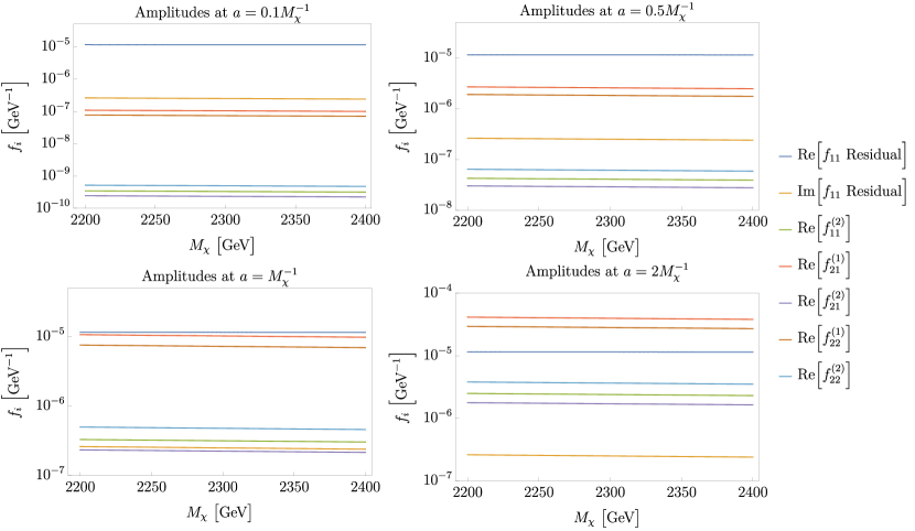
Figure 12: Numerical results for the first and second Born approximation, $f_{i}^{(1)}$ and $f_{i}^{(2)}$ respectively, to the various matrix elements $f_{11}=\langle\chi^{0}\chi^{0}|T|\chi^{0}\chi^{0}\rangle,f_{21}=\langle\chi^{0}\chi^{0}|T|\chi^{+}\chi^{-}\rangle,$ and $f_{22}=\langle\chi^{+}\chi^{-}|T|\chi^{+}\chi^{-}\rangle$, and the residual of $f_{11}$ for different values of the matching radius: $a=0.1M_{\chi}^{-1}$ (top left), $a=0.5M_{\chi}^{-1}$ (top right), $a=M_{\chi}^{-1}$ (bottom left), and $a=2M_{\chi}^{-1}$ (bottom right).

In the pure wino limit of the MSSM, $\chi^{\pm}$ and $\chi^{0}$ only couple off-diagonally via $W^{\pm}$. As a result, at lowest order, the process $\chi^{0}\chi^{0}\to\chi^{0}\chi^{0}$ occurs at one-loop level. There are twelve distinct Feynman diagrams which contribute to this process. We show the six topologies which contribute in Fig. 13 and note that there is a doubling due to the interchange of $\chi^{+}\to\chi^{-}$ and $W^{-}\to W^{+}$ in the loop. We compute the loop integrals relevant for the amplitude using PackageX Patel:2015tea ; Patel:2016fam and take the zero-momentum limit which is identical to the $\ell=0$ partial amplitude.

Figure 13: Feynman diagram topologies contributing to $\chi^{0}\chi^{0}\to\chi^{0}\chi^{0}$ scattering. Interchanging $\chi^{+}\to\chi^{-}$ and $W^{-}\to W^{+}$ in the loop leads to a doubling of diagrams.

D.2 Relating helicity and partial-wave amplitudes

While we chose to focus on the $\ell=0$ case for our wino example, in which case we can obtain the $\ell=0$ component of the full amplitude in the low-velocity limit simply by taking $p\rightarrow 0$, for more general examples we might want to carefully decompose the amplitudes computed from QFT into their partial wave components. In this subsection we review the procedure for extracting the S-matrix elements in the canonical basis given an amplitude, for particles with spin. In particular, it is often easier to compute the amplitude for states of fixed helicity and then convert it to the canonical basis. In the subsequent discussion, we will work this translation out in detail, closely following the discussion in deBoer .

We begin with one particle states with helicity $\lambda$ and momentum $\vec{p}$ which are normalized according to

$$\langle\vec{p}^{\prime},\lambda^{\prime}|\vec{p},\lambda\rangle=\tilde{\delta}(\vec{p}^{\prime}-\vec{p})\delta_{\lambda^{\prime}\lambda}=(2\pi)^{3}2E\delta^{3}(\vec{p}^{\prime}-\vec{p})\delta_{\lambda^{\prime}\lambda}$$ (213)

Two particle states are the tensor products of these states and are normalized as

$$\begin{split}&|\vec{p}_{a},\lambda_{a},\vec{p}_{b},\lambda_{b}\rangle=|\vec{p}_{a},\lambda_{a}\rangle\otimes|\vec{p}_{b},\lambda_{b}\rangle\\ &\langle\vec{p}_{a}^{\prime},\lambda_{a}^{\prime},\vec{p}_{b}^{\prime},\lambda_{b}^{\prime}|\vec{p}_{a},\lambda_{a},\vec{p}_{b},\lambda_{b}\rangle=\tilde{\delta}(\vec{p}_{a}^{\prime}-\vec{p}_{a})\tilde{\delta}(\vec{p}_{b}^{\prime}-\vec{p}_{b})\delta_{\lambda_{a}^{\prime}\lambda_{a}}\delta_{\lambda_{b}^{\prime}\lambda_{b}}\end{split}$$ (214)

In the center of momentum frame, the two particle states are defined as

$$|\vec{p}_{a},\lambda_{a},\vec{p}_{b},\lambda_{b}\rangle=\frac{1}{4\pi}\sqrt{\frac{M_{cm}}{|\vec{p}_{1}|}}|\Omega,\lambda_{1},\lambda_{2}\rangle\otimes|P\rangle$$ (215)

Where $P^{\mu}=p_{1}^{\mu}+p_{2}^{\mu}$ and $M^{2}_{cm}=P^{2}$. Furthermore, $\vec{p}_{1}=-\vec{p}_{2}$ are the momenta of particles a and b in the center of momentum frame. Likewise, $\lambda_{1}$ and $\lambda_{2}$ are the helicities of the particles in the center of momentum frame.

The state $|\Omega,\lambda_{1},\lambda_{2}\rangle$ is defined as

$$|\Omega,\lambda_{1},\lambda_{2}\rangle=\sum_{j,m}N_{j}D^{j}_{m,\lambda}(\Omega)|j,m,\lambda_{1},\lambda_{2}\rangle=\sum_{j,m}\sqrt{\frac{2j+1}{4\pi}}D^{j}_{m,\lambda}(\Omega)|j,m,\lambda_{1},\lambda_{2}\rangle$$ (216)

where $\lambda=\lambda_{1}-\lambda_{2}$.

The helicity basis states are normalized as

$$\langle j^{\prime},m^{\prime},\lambda_{1}^{\prime},\lambda_{2}^{\prime}|j,m,\lambda_{1},\lambda_{2}\rangle=\delta_{jj^{\prime}}\delta_{mm^{\prime}}\delta_{\lambda_{1}\lambda_{1}^{\prime}}\delta_{\lambda_{2}\lambda_{2}^{\prime}}$$ (217)

To determine the canonical basis states, we can again start with the states $|\phi=0,\theta=0,\lambda_{1},\lambda_{2}\rangle$. With these choices of $\phi$ and $\theta$, we know that one particle is moving in the $+z$ direction and another is moving in the $-z$ direction. Now, we can rotate this wavefunction. For a single particle, the rotation is defined by

$$\mathcal{R}(\Omega)|s,m\rangle=\sum_{m^{\prime}}D^{s}_{m^{\prime},m}(\Omega)|s,m^{\prime}\rangle$$ (218)

So, for a two particle state with the particles moving in opposite directions along the $z$ axis, we have

$$|\Omega,\lambda_{1},\lambda_{2}\rangle=\mathcal{R}(\phi,\theta,0)|\phi^{\prime}=0,\theta^{\prime}=0,\lambda_{1},\lambda_{2}\rangle=\sum_{m_{1},m_{2}}D^{s_{1}}_{m_{1},\lambda_{1}}D^{s_{2}}_{m_{2},-\lambda_{2}}|\Omega,m_{1},m_{2}\rangle$$ (219)

Since $D$ is a unitary representation, we also have

$$|\Omega,m_{1},m_{2}\rangle=\sum_{\lambda_{1},\lambda_{2}}D^{s_{1}*}_{m_{1},\lambda_{1}}D^{s_{2}*}_{m_{2},-\lambda_{2}}|\Omega,\lambda_{1},\lambda_{2}\rangle$$ (220)

Adding individual spins $s_{1}$ and $s_{2}$ to a total spin $s$ using Clebsch-Gordan coefficients, we have

$$|\Omega,s,m_{s}\rangle=\sum_{m_{1},m_{2}}\langle s_{1},m_{1},s_{2},m_{2}|s,m_{s}\rangle|\Omega,m_{1},m_{2}\rangle$$ (221)

Furthermore, the spherical harmonics are defined as

$$Y_{l,m_{l}}(\Omega)=\langle\theta,\phi|l,m_{l}\rangle$$ (222)

Using this, the states can be written as

$$|\Omega,s,m_{s}\rangle=\sum_{l,m_{l}}Y_{l,m_{l}}(\Omega)^{*}|l,m_{l},s,m_{s}\rangle\quad\longleftrightarrow\quad|l,m_{l},s,m_{s}\rangle=\int d\Omega Y_{l,m_{l}}(\Omega)|\Omega,s,m_{s}\rangle$$ (223)

Finally, we couple spin and orbital angular momentum to form total angular momentum states. Using Clebsch-Gordan coefficients to couple, we have

$$|j,m,l,s\rangle=\sum_{m_{l},m_{s}}\langle l,m_{l},s,m_{s}|j,m\rangle|l,m_{l},s,m_{s}\rangle$$ (224)

Next, writing $|\Omega,m_{1},m_{2}\rangle$ in terms of $|j,m,\lambda_{1},\lambda_{2}\rangle$, we have

$$|\Omega,m_{1},m_{2}\rangle=\sum_{\lambda_{1},\lambda_{2}}\sum_{j,m}\sqrt{\frac{2j+1}{4\pi}}D^{s_{1}*}_{m_{1},\lambda_{1}}D^{s_{2}*}_{m_{2},-\lambda_{2}}D^{j}_{m,\lambda}|j,m,\lambda_{1},\lambda_{2}\rangle$$ (225)

Using the following identities

$$\begin{split}D^{j_{1}}_{m_{1},m_{1}^{\prime}}D^{j_{2}}_{m_{2},m_{2}^{\prime}}&=\sum_{j_{3},m_{3},m_{3}^{\prime}}\langle j_{1},m_{1},j_{2},m_{2}|j_{3},m_{3}\rangle\langle j_{1},m_{1}^{\prime},j_{2},m_{2}^{\prime}|j_{3},m_{3}^{\prime}\rangle D^{j_{3}}_{m_{3},m_{3}^{\prime}}\\ D^{j_{1}}_{m_{1},m_{1}^{\prime}}D^{j_{3}*}_{m_{3},m_{3}^{\prime}}&=\sum_{j_{2},m_{2},m_{2}^{\prime}}\frac{2j_{2}+1}{2j_{3}+1}\langle j_{1},m_{1},j_{2},m_{2}|j_{3},m_{3}\rangle\langle j_{1},m_{1}^{\prime},j_{2},m_{2}^{\prime}|j_{3},m_{3}^{\prime}\rangle D^{j_{2}*}_{m_{2},m_{2}^{\prime}}\\ \end{split}$$ (226)

we can simplify the product of three Wigner-D functions and find

$$\begin{split}|\Omega,m_{1},m_{2}\rangle&=\sum_{\lambda_{1},\lambda_{2}}\sum_{j,m}\sum_{l,m_{l}}\sum_{s,m_{s}}\sqrt{\frac{2l+1}{2j+1}}\langle s,m_{s},l,m_{l}|j,m\rangle\langle s,\lambda,l,0|j,\lambda\rangle\\ &\times\langle s_{1},m_{1},s_{2},m_{2}|s,m_{s}\rangle\langle s_{1},\lambda_{1},s_{2},-\lambda_{2}|s,\lambda\rangle Y_{l,m_{l}}^{*}|j,m,\lambda_{1},\lambda_{2}\rangle\end{split}$$ (227)

Substituting this into the expression for the states $|j,m,l,s\rangle$, we find

$$\begin{split}|j,m,l,s\rangle&=\sum_{m_{l},m_{s}}\sum_{m_{1},m_{2}}\int d\Omega Y_{l,m_{l}}\langle l,m_{l},s,m_{s}|j,m\rangle\langle s_{1},m_{1},s_{2},m_{2}|s,m_{s}\rangle\\ &\times\sum_{\lambda_{1},\lambda_{2}}\sum_{j^{\prime},m^{\prime}}\sum_{l^{\prime},m_{l}^{\prime}}\sum_{s^{\prime},m_{s}^{\prime}}\sqrt{\frac{2l^{\prime}+1}{2j^{\prime}+1}}\langle s^{\prime},m_{s}^{\prime},l^{\prime},m_{l}^{\prime}|j^{\prime},m^{\prime}\rangle\langle s,\lambda,l^{\prime},0|j^{\prime},\lambda\rangle\\ &\times\langle s_{1},m_{1},s_{2},m_{2}|s^{\prime},m_{s}^{\prime}\rangle\langle s_{1},\lambda_{1},s_{2},-\lambda_{2}|s^{\prime},\lambda\rangle Y_{l^{\prime},m_{l}^{\prime}}^{*}|j^{\prime},m^{\prime},\lambda_{1},\lambda_{2}\rangle\end{split}$$ (228)

Integrating the spherical harmonics and using various Clebsch-Gordan identities to simplify these sums, we arrive at

$$|j,m,l,s\rangle=(-1)^{l+s-j}\sum_{\lambda_{1},\lambda_{2}}\sqrt{\frac{2l+1}{2j+1}}\langle s,\lambda,l,0|j,\lambda\rangle\langle s_{1},\lambda_{1},s_{2},-\lambda_{2}|s,\lambda\rangle|j,m,\lambda_{1},\lambda_{2}\rangle$$ (229)

Next, we will investigate the invariant amplitude which we decompose as follows

$$\mathcal{M}_{fi}=(4\pi)^{2}\frac{M_{cm}}{\sqrt{|\vec{p}_{i}||\vec{p}_{f}|}}\langle\Omega,\lambda_{3},\lambda_{4}|T(M_{cm})|0,0,\lambda_{1},\lambda_{2}\rangle$$ (230)

Enforcing conservation of total angular momentum and writing the amplitude in terms of helicity basis states, we have

$$\mathcal{M}_{fi}=4\pi\frac{M_{cm}}{\sqrt{|\vec{p}_{i}||\vec{p}_{f}|}}\sum_{j}(2j+1)D^{j*}_{\lambda_{i},\lambda_{f}}(\Omega)\langle j,\lambda_{i},\lambda_{3},\lambda_{4}|T(M_{cm})|j,\lambda_{i},\lambda_{1},\lambda_{2}\rangle$$ (231)

where $\lambda_{i}=\lambda_{1}-\lambda_{2}$. We also define $\lambda_{f}=\lambda_{3}-\lambda_{4}$ for future reference.

With the invariant amplitude written as a sum over matrix elements in the helicity basis, we can now invert this relationship. Extracting the partial amplitude in the helicity basis, we find

$$\langle j,m,\lambda_{3},\lambda_{4}|T(M_{cm})|j,m,\lambda_{1},\lambda_{2}\rangle=\frac{\sqrt{|\vec{p}_{i}||\vec{p}_{f}|}}{(4\pi)^{2}M_{cm}}\int d\Omega D^{j}_{m,m^{{}^{\prime}}}(\Omega)\mathcal{M}_{fi}$$ (232)

Finally, we can convert from the helicity basis to the canonical basis using our basis change relations and we find

$$\begin{split}\langle j,m,\ell^{\prime},s^{\prime}|T(M_{cm})|j,m,\ell,s\rangle&=(-1)^{\ell+s-j}(-1)^{\ell^{\prime}+s^{\prime}-j}\sum_{\lambda_{1},\lambda_{2}}\sum_{\lambda_{3},\lambda_{4}}\sqrt{\frac{2\ell^{\prime}+1}{2j+1}}\sqrt{\frac{2\ell+1}{2j+1}}\\ &\times\langle s^{\prime},\lambda_{f},\ell^{\prime},0|j,\lambda_{f}\rangle\langle s_{3},\lambda_{3},s_{4},-\lambda_{4}|s^{\prime},\lambda_{f}\rangle\\ &\times\langle s,\lambda_{i},\ell,0|j,\lambda_{i}\rangle\langle s_{1},\lambda_{1},s_{2},-\lambda_{2}|s,\lambda_{i}\rangle\\ &\times\langle j,m,\lambda_{3},\lambda_{4}|T(M_{cm})|j,m,\lambda_{1},\lambda_{2}\rangle\end{split}$$ (233)

Here we have enforced conservation of total angular momentum and defined $\lambda_{i}=\lambda_{1}-\lambda_{2}$ and $\lambda_{f}=\lambda_{3}-\lambda_{4}$ as before.

Appendix E Supplemental results for the wino example

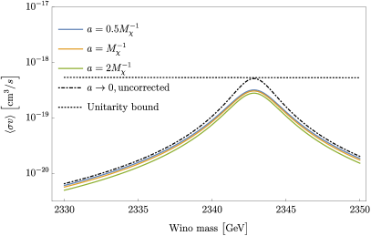
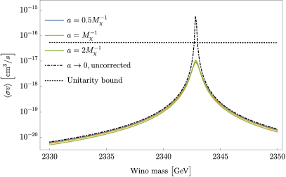
Figure 14: Colored lines show the Sommerfeld-enhanced annihilation cross section for wino dark matter, using the corrected expression derived in this work, for different choices of the matching radius $a$. The dot-dashed black line shows the result of computing the uncorrected Sommerfeld-enhanced annihilation cross section. The relative velocity between DM particles is taken to be $v=10^{-4}$ (left) or $v=10^{-6}$ (right). The dotted black line indicates the unitarity bound on the annihilation cross section. Results in this figure are computed using the tree-level wino potential.

E.1 LO vs NLO potential

In this subsection we show the effect of using Eq. 163 for the wino potential, omitting the corrections described in Eq. 164; we also do not include these corrections in $f_{s,\ell}$. We otherwise proceed as described in the main text. Fig. 14 shows the regulated and unregulated cross sections near the resonance point, and can be compared directly with Fig. 10. We see that the results are qualitatively very similar; the only major difference is the position of the resonance, which shifts upward in mass by about 140 GeV (from around 2340 GeV to 2480 GeV) when the NLO corrections are included. The shift of the resonance is a known effect, already noted in Refs. Beneke:2019qaa ; Urban:2021cdu . However, it is worth noting that the resonance position is quite sensitive to the details of the real potential, and so small real/Hermitian corrections to $f_{s,\ell}$ can also noticeably shift the resonance peak; choosing a convention where $V_{\text{long}}(r)$ is $a$-dependent will similarly lead to $a$-dependent shifts in the resonances. We will explore these effects further in the following subsections.

E.2 Effect of including one-loop correction to $(f_{s})_{11}$

The NLO potential we employ still has zero $11$ component. We computed the one-loop contribution to the $11$ component for $\ell=0$ through a perturbative QFT calculation; the numerical results for this amplitude are shown in Fig. 12. We used this calculation to cross-check both (1) that the imaginary part of this amplitude is related to the contribution to $f_{s,\ell}$ from annihilation as described in App. C, and (2) that the real part of this amplitude matches closely to the 2nd Born approximation from the tree-level potential, which we expect to be the dominant contribution, once it is rescaled by a factor $32\pi M_{\chi}$ as described in App. C. The residual part of this amplitude (not accounted for by the Born approximation) can then be rescaled appropriately and added to $\hat{f}_{s}$ as a short-distance correction to the elastic scattering.

In Fig. 15 we show the results of including this term relative to our baseline calculation with the NLO potential, choosing $a=1/M_{\chi}$ for clarity (since we have already demonstrated the result is largely independent of $a$; we have checked this remains true when the residual term is added). We observe a shift in the resonance position, as expected, but to a much lesser degree than that induced by the NLO correction to the potential ($\sim 3$ GeV vs. 140 GeV). Otherwise the results are very similar – in particular, the cross section at the peak is similar in the two cases, despite the shift in peak position – justifying our neglect of this term (and real corrections of similar size to the other components of $f_{s,\ell}$).

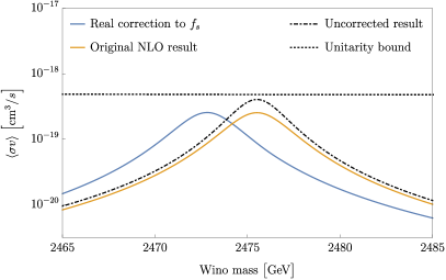
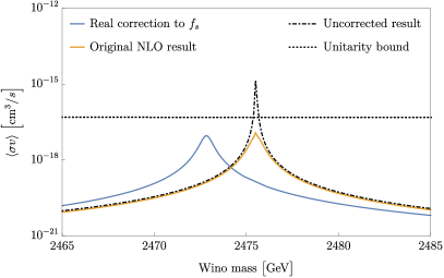
Figure 15: The Sommerfeld-enhanced annihilation cross section for wino dark matter, using the corrected expression derived in this work, with (blue line) or without (orange line) including the one-loop correction to the real part of the short-distance scattering amplitude $(f_{s,0})_{11}$. The dot-dashed black line shows the result of computing the uncorrected Sommerfeld-enhanced annihilation cross section, which is independent of the real part of $(f_{s,0})_{11}$. The relative velocity between DM particles is taken to be $v=10^{-4}$ (left) or $v=10^{-6}$ (right). The dotted black line indicates the unitarity bound on the annihilation cross section. Results in this figure are computed using the NLO potential for the wino and taking the matching radius to be $a=1/M_{\chi}$.

E.3 Results with modified convention for $V_{\text{long}}(r)$ at $r<a$

To see how the $a$-independence of the final result emerges in a case where the resonance positions are $a$-dependent, and to demonstrate the convention-independence of the final result, in this section we show results derived by fixing $V_{\text{long}}(r)=0$ for $r<a$. This means that we can use the simplified expression for $\kappa_{\ell}$ discussed below Eq. 141, which in our $N=2$, $M=1$, $\ell=0$ case becomes:

$$\kappa^{-1}=f_{s}^{-1}-\begin{pmatrix}\sqrt{p_{1}}&0\\ 0&(p_{1}^{2}-2M_{\chi}\Delta)^{1/4}\end{pmatrix}\alpha_{\tilde{G}_{\ell}}(a).$$ (234)

However, we must now include in $f_{s}$ the contribution from the wino potential for $r<a$. Throughout this section, we employ the LO potential of Eq. 163, and compute the second Born approximation for the contributions to $f_{s,\ell}$ from this potential within the matching radius, as detailed in App. D. The results of this section can thus be compared directly to those obtained for the LO case with our previous convention, shown in the first subsection of this appendix.

We plot in Fig. 16 both the full annihilation cross section, and the cross section obtained using the uncorrected Sommerfeld enhancement $\sigma_{\ell,0}$, as a function of the wino mass $M_{\chi}$, for two different velocities as previously. We observe that the results still converge well for small $a$, although the deviation for $a=2/M_{\chi}$ is more pronounced than with our previous convention (this is not unexpected, as in this convention we make the additional approximation of treating the potential for $r<a$ perturbatively).

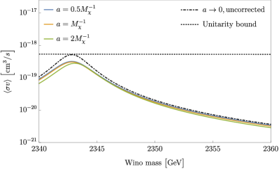
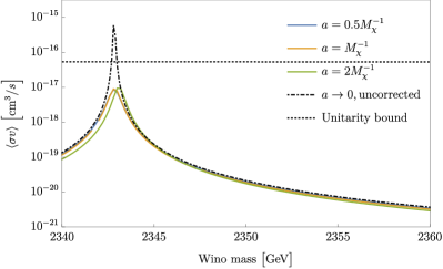
Figure 16: The Sommerfeld-enhanced annihilation cross section for wino dark matter, using the corrected expression derived in this work, for different choices of the matching radius $a$, in the convention where we fix $V_{\text{long}}(r)=0$ for $r<a$. The dot-dashed black line shows the result of computing the uncorrected Sommerfeld enhancement (i.e. to leading order in the short-range matrix element) with $a\rightarrow 0$ in the evaluation of $\Sigma_{0,\ell}$. The dotted black line indicates the unitarity bound on the annihilation cross section. The relative velocity between DM particles is taken to be $v=10^{-4}$ (left), or $v=10^{-7}$ (right). All calculations for this figure were performed using the tree-level wino potential.

The ingredients computed from the long-range potential, i.e. the $\sigma_{0}$, $\sigma_{\pm}$ and $\alpha_{\tilde{G}_{\ell}}(a)$ factors, are shown as a function of $a$ and $M_{\chi}$ in Fig. 17. Note that the resonances in the uncorrected Sommerfeld factors (left panel) are markedly displaced for different choices of $a$, in contrast to the resonances in the corrected cross section (Fig. 16). Similarly, in the right panel we see that $\alpha_{\tilde{G}_{\ell}}(a)$ has pronounced features associated with the resonances in the uncorrected Sommerfeld enhancement. This serves as a cross-check on the validity of our method: the inclusion of $a$-dependence in $f_{s,\ell}$ and $\alpha_{\tilde{G}_{\ell}}(a)$ is correctly canceling the $a$-dependence in $\Sigma_{0,\ell}$, and shifting the resonance peaks (for different choices of $a$) to coincide with each other in the final corrected result.

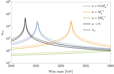
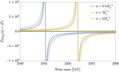
Figure 17: Left panel: Uncorrected Sommerfeld factors $\sigma_{0}$ (solid lines) and $\sigma_{\pm}$ (dashed lines), as a function of the wino mass, for different choices of $a$, at $v_{\text{rel}}=10^{-7}$. The black lines correspond to the limit $a\rightarrow 0$. Note that the resonance is shifted beyond the right-hand edge of the plot in the case of $a=2/M_{\chi}$. Right panel: components of the real symmetric matrix $\tilde{P}(\alpha_{\tilde{G}_{\ell}}(a)+i\tilde{P})$, for $v_{\text{rel}}=10^{-7}$. Solid, dashed, and dotted lines show the values of the $11$, $12$, and $22$ components respectively. All calculations for this figure were performed using the tree-level wino potential.

E.4 $p$-wave case

It is straightforward to extend our calculation to the $p$-wave case; however, in numerical testing, we have not found parameter points where the uncorrected result approaches or exceeds the unitarity bound for the $p$-wave case, meaning that the corrected result is rather trivial for all points we have tested (because it agrees closely with the uncorrected result). Nonetheless, we include here the necessary inputs to perform the $p$-wave calculation.

Choosing $\ell=1$ for the wino, and choosing a convention where $\sigma_{0}$ is real and $\sigma_{\pm}$ is purely imaginary, the $p$-wave annihilation cross section is given by:

$$\sigma_{\text{ann}}v_{\text{rel}} =\frac{24\pi i}{M_{\chi}}\begin{pmatrix}\sigma_{0}&-\sigma_{\pm}\end{pmatrix}\left[1+ip_{1}\kappa_{1}^{\dagger}\begin{pmatrix}\sigma_{0}^{2}&-\sigma_{0}\sigma_{\pm}\\ \sigma_{0}\sigma_{\pm}&-\sigma_{\pm}^{2}\end{pmatrix}\right]^{-1}(\kappa_{1}^{\dagger}-\kappa_{1})$$

$$\times\left[1-ip_{1}\begin{pmatrix}\sigma_{0}^{2}&-\sigma_{0}\sigma_{\pm}\\ \sigma_{0}\sigma_{\pm}&-\sigma_{\pm}^{2}\end{pmatrix}\kappa_{1}\right]^{-1}\begin{pmatrix}\sigma_{0}\\ \sigma_{\pm}\end{pmatrix}.$$ (235)

Writing $\kappa_{1}=\begin{pmatrix}\kappa_{11}&\kappa_{12}\\ \kappa_{21}&\kappa_{22}\end{pmatrix}$ and explicitly performing the matrix inversion yields:

$$\sigma_{\text{ann}}v_{\text{rel}} =-\frac{24\pi i}{M_{\chi}}\frac{\left[(\kappa_{11}-\kappa_{11}^{*})\sigma_{0}^{2}-(\kappa_{22}-\kappa_{22}^{*})\sigma_{\pm}^{2}+(\kappa_{12}-\kappa_{21}-\kappa_{21}^{*}+\kappa_{12}^{*})\sigma_{0}\sigma_{\pm}\right]}{\left|i+p_{1}\left(\sigma_{0}^{2}\kappa_{11}-\sigma_{\pm}^{2}\kappa_{22}+\sigma_{0}\sigma_{\pm}(\kappa_{12}-\kappa_{21})\right)\right|^{2}}$$

$$=\frac{48\pi}{M_{\chi}}\frac{\left[\sigma_{0}^{2}\text{Im}\kappa_{11}-\sigma_{\pm}^{2}\text{Im}\kappa_{22}-i\sigma_{0}\sigma_{\pm}\text{Re}(\kappa_{12}-\kappa_{21})\right]}{\left|i+p_{1}\left(\sigma_{0}^{2}\kappa_{11}-\sigma_{\pm}^{2}\kappa_{22}+\sigma_{0}\sigma_{\pm}(\kappa_{12}-\kappa_{21})\right)\right|^{2}}.$$ (236)

It may be surprising to see a dependence on the real part of the off-diagonal terms in the numerator, but due to the momentum dependence of $\kappa_{1}$, in the case where the long-range potential can be neglected, the off-diagonal terms in the contribution from the optical theorem are actually real (but $\bar{\Gamma}_{1}$ is non-Hermitian as required because it is antisymmetric). Specifically, from the results of App. C we can take the contribution to $f_{s,1}$ from annihilation to be:

$$f_{s,1} =-\frac{1}{2}\begin{pmatrix}1&0\\ 0&-1\end{pmatrix}\frac{\mu}{2i\pi}\frac{1}{3}\frac{1}{(2\mu)^{2}}\frac{28\pi\alpha_{W}^{2}}{9(2\mu)^{2}}\begin{pmatrix}|p_{1}|^{2}&\frac{1}{\sqrt{2}}p_{1}^{*}p_{2}\\ \frac{1}{\sqrt{2}}p_{2}^{*}p_{1}&\frac{3}{2}|p_{2}|^{2}\end{pmatrix}$$

$$=\frac{7i}{54}\frac{\alpha_{W}^{2}}{(2\mu)^{3}}\begin{pmatrix}|p_{1}|^{2}&\frac{1}{\sqrt{2}}p_{1}^{*}p_{2}\\ -\frac{1}{\sqrt{2}}p_{2}^{*}p_{1}&-\frac{3}{2}|p_{2}|^{2}\end{pmatrix}.$$ (237)

Appendix F Generalization of multi-state results to a complex long-range potential

In Sec. 3 we assumed that $V_{\text{long}}(r)$ was real and symmetric, which is the case for most commonly-considered examples in the literature. More generally, $V_{\text{long}}(r)$ can be Hermitian but complex; in this appendix, we discuss how to generalize the results of Sec. 3 to this case.

For a complex potential, it is not generally true that the real and imaginary parts of a solution to the Schrödinger solution are separately solutions, so we cannot decompose $\tilde{w}_{\ell}(r)$ in terms of the real solutions $\tilde{G}_{\ell}(r)$ and $\tilde{F}_{\ell}(r)$. However, we can simply work with $\tilde{w}_{\ell}(r)$ itself, as the definitions of $w_{\ell}(r)$ and $\tilde{w}_{\ell}(r)$ do not rely on the potential being real.

Furthermore, given any two solutions $u(r)$ and $v(r)$, $u^{\dagger}(r)v^{\prime}(r)-(u^{\dagger}(r))^{\prime}v(r)$ provides a conserved Wronskian, but in the main text we derived other Wronskian relations by conjugating one of the solutions (or breaking one of the solutions into its real and imaginary parts); these relations are no longer valid, so some caution is needed. It is easy to check that the Wronskian relation for $\hat{W}_{ij}$ given in Sec. 3.3 is of the form $u^{\dagger}(r)v^{\prime}(r)-(u^{\dagger}(r))^{\prime}v(r)$, and so remains valid for a complex potential, yielding:

$$Q_{\ell}^{\dagger}(\tilde{P}^{\dagger})^{2(\ell+1)}=(1-2iP^{2}f_{0,\ell}^{\dagger})P^{2}f_{1,\ell}\tilde{P}^{2}.$$ (238)

Now note that $S_{0,\ell}=1+2iPf_{0,\ell}P$, so $PS_{0,\ell}^{\dagger}P^{-1}=1-2iP^{2}f_{0,\ell}^{\dagger}$, and thus we have $Q_{\ell}^{\dagger}(\tilde{P}^{\dagger})^{2(\ell+1)}=PS_{0,\ell}^{\dagger}Pf_{1,\ell}\tilde{P}^{2}$. But as $S_{0,\ell}$ is unitary, this implies

$$Pf_{1,\ell}\tilde{P}^{2}=S_{0,\ell}P^{-1}Q_{\ell}^{\dagger}(\tilde{P}^{\dagger})^{2(\ell+1)}.$$ (239)

The first equality in Eq. 123 is purely a corollary of writing the full solution as $w_{\ell}(r)+\tilde{w}_{\ell}(r)R_{\ell}$, so we have:

$$S_{\ell} =S_{0,\ell}+2iPf_{1,\ell}\tilde{P}^{2}R_{\ell}P^{-1}$$

$$=S_{0,\ell}\left[1+2iP^{-1}Q_{\ell}^{\dagger}(\tilde{P}^{\dagger})^{2(\ell+1)}R_{\ell}P^{-1}\right].$$ (240)

This is an alternate (actually somewhat simpler) proof of Eq. 127 that does not rely on the potential being real.

Thus writing down the full $S$-matrix element just requires us to determine $R_{\ell}$. The equivalent of Eq. 132, without separating $\tilde{w}_{\ell}(r)$ into real and imaginary components, is:

$$\alpha_{w_{\ell}}(0)=\tilde{P}Q_{\ell},\quad\beta_{w_{\ell}}(0)=0,\quad\beta_{\tilde{w}_{\ell}}(0)=-\tilde{P}^{2\ell+1}.$$ (241)

The matching at $r=a$ gives $\tilde{P}f_{s,\ell}\tilde{P}\alpha_{\ell}(a)=-\beta_{\ell}(a)$ as in Eq. 134, which becomes:

$$\tilde{P}f_{s,\ell}\tilde{P}(\alpha_{w_{\ell}}(a)+\alpha_{\tilde{w}_{\ell}}(a)R_{\ell})=-(\beta_{w_{\ell}}(a)+\beta_{\tilde{w}_{\ell}}(a)R_{\ell})$$

$$\Rightarrow R_{\ell}=-\left[\beta_{\tilde{w}_{\ell}}(a)+\tilde{P}f_{s,\ell}\tilde{P}\alpha_{\tilde{w}_{\ell}}(a)\right]^{-1}\left(\tilde{P}f_{s,\ell}\tilde{P}\alpha_{w_{\ell}}(a)+\beta_{w_{\ell}}(a)\right)$$ (242)

The relation that $\beta_{w_{\ell}}(a)=-\tilde{P}f_{b,\ell}\tilde{P}\alpha_{w_{\ell}}(a)$ does not depend on the properties of the potential, and similarly $\tilde{P}Q_{\ell}=\alpha_{w_{\ell}}(0)=\alpha_{b,\ell}(0)\tilde{P}^{-1}\alpha_{w_{\ell}}(a)$ still holds. So we can write $\hat{f}_{s}=f_{s}-f_{b}$ as previously, and thus:

$$R_{\ell} =-\left[\beta_{\tilde{w}_{\ell}}(a)+\tilde{P}f_{b,\ell}\tilde{P}\alpha_{\tilde{w}_{\ell}}(a)+\tilde{P}\hat{f}_{s,\ell}\tilde{P}\alpha_{\tilde{w}_{\ell}}(a)\right]^{-1}\tilde{P}\hat{f}_{s,\ell}\tilde{P}\alpha_{w_{\ell}}(a)$$

$$=-\left[\left(\tilde{P}\hat{f}_{s,\ell}\tilde{P}\right)^{-1}\left(\beta_{\tilde{w}_{\ell}}(a)+\tilde{P}f_{b,\ell}\tilde{P}\alpha_{\tilde{w}_{\ell}}(a)\right)+\alpha_{\tilde{w}_{\ell}}(a)\right]^{-1}\tilde{P}\alpha_{b,\ell}(0)^{-1}\tilde{P}Q_{\ell}$$

$$=-\left[\alpha_{b,\ell}(0)\tilde{P}^{-1}\left(\tilde{P}\hat{f}_{s,\ell}\tilde{P}\right)^{-1}\left(\beta_{\tilde{w}_{\ell}}(a)+\tilde{P}f_{b,\ell}\tilde{P}\alpha_{\tilde{w}_{\ell}}(a)\right)+\alpha_{b,\ell}(0)\tilde{P}^{-1}\alpha_{\tilde{w}_{\ell}}(a)\right]^{-1}\tilde{P}Q_{\ell}.$$ (243)

We note that the coefficient of the $\hat{f}_{s}^{-1}$ term in the denominator, the $\alpha_{\tilde{w}_{\ell}}(a)$ term in the denominator, and the numerator can all be computed solely from the long-range potential and the matching radius.

Let us now define $\Sigma_{0,\ell}=\tilde{P}^{2}Q_{\ell}P^{-2}$ as previously, and:

$$-\kappa_{\ell}^{-1} \equiv\tilde{P}\left[\alpha_{b,\ell}(0)\tilde{P}^{-1}\left(\tilde{P}\hat{f}_{s,\ell}\tilde{P}\right)^{-1}\left(\beta_{\tilde{w}_{\ell}}(a)+\tilde{P}f_{b,\ell}\tilde{P}\alpha_{\tilde{w}_{\ell}}(a)\right)\right.$$

$$+\left.\alpha_{b,\ell}(0)\tilde{P}^{-1}\alpha_{\tilde{w}_{\ell}}(a)\right](\tilde{P}^{\dagger})^{-2\ell}-i\Sigma_{0,\ell}P^{2}\Sigma_{0,\ell}^{\dagger}.$$ (244)

Then we have:

$$R_{\ell}=(\tilde{P}^{\dagger})^{-2\ell}\left[\kappa_{\ell}^{-1}-i\Sigma_{0,\ell}P^{2}\Sigma_{0,\ell}^{\dagger}\right]^{-1}\tilde{P}^{2}Q_{\ell},$$ (245)

and so the $S$-matrix is given by:

$$S_{\ell}=S_{0,\ell}\left(1+2iP\Sigma_{0,\ell}^{\dagger}\left[\kappa_{\ell}^{-1}-i\Sigma_{0,\ell}P^{2}\Sigma_{0,\ell}^{\dagger}\right]^{-1}\Sigma_{0,\ell}P\right).$$ (246)

This is exactly the form given in Eq. 141, but with a modified/generalized definition for $\kappa_{\ell}$. Note that $\kappa_{\ell}^{-1}$ can still be expressed in terms of $\hat{f}_{s}^{-1}$, a multiplicative factor determined from the long-range potential, and an additive factor determined from the long-range potential. The subsequent discussion in the main text then carries over to this more general case, with the appropriate replacement of $\kappa_{\ell}$.

For illustration, let us work out $\kappa_{\ell}$ under the convention where $V_{\text{long}}(r)=0$ for $r<a$, so that we have $\alpha_{b,\ell}(0)=\tilde{P}$, $f_{b,\ell}=0$, $\beta_{\tilde{w}_{\ell}}(a)=-\tilde{P}^{2\ell+1}$, $\alpha_{\tilde{w}_{\ell}}(a)=\alpha_{\tilde{w}_{\ell}}(0)$. Then Eq. 244 becomes:

$$\kappa_{\ell}^{-1} \equiv\hat{f}_{s,\ell}^{-1}\tilde{P}^{2\ell}(\tilde{P}^{\dagger})^{-2\ell}-\tilde{P}\alpha_{\tilde{w}_{\ell}}(a)(\tilde{P}^{\dagger})^{-2\ell}+i\Sigma_{0,\ell}P^{2}\Sigma_{0,\ell}^{\dagger}.$$ (247)

As shown in Eq. 195, in the case of a real and symmetric potential $\alpha_{\tilde{G}_{\ell}}(a)=\alpha_{\tilde{w}_{\ell}}(a)-i\alpha_{w_{\ell}}(a)\Sigma_{0,\ell}^{\dagger}(\tilde{P}^{\dagger})^{2\ell}$, and with the present convention we have $\alpha_{w_{\ell}}(a)=\tilde{P}Q_{\ell}$, so we obtain:

$$\alpha_{\tilde{G}_{\ell}}(a) =\alpha_{\tilde{w}_{\ell}}(a)-i\tilde{P}^{-1}\Sigma_{0,\ell}P^{2}\Sigma_{0,\ell}^{\dagger}(\tilde{P}^{\dagger})^{2\ell}$$

$$\Rightarrow\tilde{P}\alpha_{\tilde{G}_{\ell}}(a)(\tilde{P}^{\dagger})^{-2\ell} =\tilde{P}\alpha_{\tilde{w}_{\ell}}(a)(\tilde{P}^{\dagger})^{-2\ell}-i\Sigma_{0,\ell}P^{2}\Sigma_{0,\ell}^{\dagger}.$$ (248)

Thus we recover our previously derived expression for $\kappa_{\ell}^{-1}$ in terms of $\alpha_{\tilde{G}_{\ell}}(a)$ in the case of a real symmetric potential, under this convention, as discussed below Eq. 141.

References

- (1) J. Hisano, S. Matsumoto and M. M. Nojiri, Unitarity and higher order corrections in neutralino dark matter annihilation into two photons, Phys. Rev. D 67 (2003) 075014 [hep-ph/0212022].
- (2) J. Hisano, S. Matsumoto and M. M. Nojiri, Explosive dark matter annihilation, Phys. Rev. Lett. 92 (2004) 031303 [hep-ph/0307216].
- (3) J. Hisano, S. Matsumoto, M. M. Nojiri and O. Saito, Non-perturbative effect on dark matter annihilation and gamma ray signature from galactic center, Phys. Rev. D 71 (2005) 063528 [hep-ph/0412403].
- (4) A. Sommerfeld, Über die Beugung und Bremsung der Elektronen, Annalen Phys. 403 (1931) 257.
- (5) N. Arkani-Hamed, D. P. Finkbeiner, T. R. Slatyer and N. Weiner, A Theory of Dark Matter, Phys. Rev. D 79 (2009) 015014 [0810.0713].
- (6) R. Iengo, Sommerfeld enhancement: General results from field theory diagrams, JHEP 05 (2009) 024 [0902.0688].
- (7) S. Cassel, Sommerfeld factor for arbitrary partial wave processes, J. Phys. G 37 (2010) 105009 [0903.5307].
- (8) T. R. Slatyer, The Sommerfeld enhancement for dark matter with an excited state, JCAP 02 (2010) 028 [0910.5713].
- (9) K. Blum, R. Sato and T. R. Slatyer, Self-consistent Calculation of the Sommerfeld Enhancement, JCAP 06 (2016) 021 [1603.01383].
- (10) T. L. Trueman, Energy level shifts in atomic states of strongly-interacting particles, Nucl. Phys. 26 (1961) 57.
- (11) J. Carbonell, J.-M. Richard and S. Wycech, On the relation between protonium level shifts and nucleon - anti-nucleon scattering amplitudes, Z. Phys. A343 (1992) 325.
- (12) J. Carbonell and K. V. Protasov, Annihilation of ultra low energy antiprotons, Hyp. Int. 76 (1993) 327.
- (13) J. Carbonell and K. V. Protasov, Annihilation of slow anti-protons in flight and in traps, Z. Phys. A355 (1996) 87.
- (14) J. Carbonell, K. V. Protasov and A. Zenoni, anti-p p low-energy parameters from annihilation cross-section data, Phys. Lett. B397 (1997) 345 [nucl-th/9806032].
- (15) K. V. Protasov, G. Bonomi, E. Lodi Rizzini and A. Zenoni, Anti-proton annihilation on light nuclei at very low- energies, Eur. Phys. J. A7 (2000) 429 [nucl-th/9911005].
- (16) X. Kong and F. Ravndal, Proton proton scattering lengths from effective field theory, Phys. Lett. B 450 (1999) 320 [nucl-th/9811076].
- (17) X. Kong and F. Ravndal, Proton proton fusion in leading order of effective field theory, Nucl. Phys. A 656 (1999) 421 [nucl-th/9902064].
- (18) E. Braaten, E. Johnson and H. Zhang, Zero-range effective field theory for resonant wino dark matter. Part I. Framework, JHEP 11 (2017) 108 [1706.02253].
- (19) E. Braaten, E. Johnson and H. Zhang, Zero-range effective field theory for resonant wino dark matter. Part II. Coulomb resummation, JHEP 02 (2018) 150 [1708.07155].
- (20) E. Braaten, E. Johnson and H. Zhang, Zero-range effective field theory for resonant wino dark matter. Part III. Annihilation effects, JHEP 05 (2018) 062 [1712.07142].
- (21) X. Chu, C. Garcia-Cely and H. Murayama, A Practical and Consistent Parametrization of Dark Matter Self-Interactions, JCAP 06 (2020) 043 [1908.06067].
- (22) A. Kamada, T. Kuwahara and A. Patel, Quantum theory of dark matter scattering, JHEP 11 (2023) 105 [2303.17961].
- (23) P. Agrawal, A. Parikh and M. Reece, Systematizing the Effective Theory of Self-Interacting Dark Matter, JHEP 10 (2020) 191 [2003.00021].
- (24) A. Parikh, The singularity structure of quantum-mechanical potentials, Phys. Rev. D 104 (2021) 036005 [2012.11606].
- (25) H. A. Bethe, Theory of the Effective Range in Nuclear Scattering, Phys. Rev. 76 (1949) 38.
- (26) G. F. Chew and M. L. Goldberger, On the Analysis of Nucleon-Nucleon Scattering Experiments, Phys. Rev. 75 (1949) 1637.
- (27) H. A. Bethe and P. Morrison, Elementary Nuclear Theory. 1956.
- (28) M. L. Goldberger and K. M. Watson, Collision Theory. 1964.
- (29) P. Asadi, M. Baumgart, P. J. Fitzpatrick, E. Krupczak and T. R. Slatyer, Capture and Decay of Electroweak WIMPonium, JCAP 02 (2017) 005 [1610.07617].
- (30) V. S. Popov and V. D. Mur, Coulomb problem with short-range forces (exact solution), Sov. J. Nucl. Phys. 42 (1985) 930.
- (31) M. M. Flores and K. Petraki, Unitarity in the non-relativistic regime and implications for dark matter, Phys. Lett. B 858 (2024) 139022 [2405.02222].
- (32) A. Kamada, S. Kobayashi and T. Kuwahara, Perturbative unitarity of strongly interacting massive particle models, JHEP 02 (2023) 217 [2210.01393].
- (33) D. Gaspard and J.-M. Sparenberg, Effective-range function methods for charged particle collisions, Phys. Rev. C 97 (2018) 044003 [1801.08980].
- (34) M. Beneke, R. Szafron and K. Urban, Wino potential and Sommerfeld effect at NLO, Phys. Lett. B 800 (2020) 135112 [1909.04584].
- (35) K. Urban, NLO electroweak potentials for minimal dark matter and beyond, JHEP 10 (2021) 136 [2108.07285].
- (36) M. Beneke, C. Hellmann and P. Ruiz-Femenia, Non-relativistic pair annihilation of nearly mass degenerate neutralinos and charginos III. Computation of the Sommerfeld enhancements, JHEP 05 (2015) 115 [1411.6924].
- (37) X. Cui and F. Luo, Final state Sommerfeld effect on dark matter relic abundance, JHEP 01 (2021) 156 [2009.14591].
- (38) M. Cirelli, A. Strumia and M. Tamburini, Cosmology and Astrophysics of Minimal Dark Matter, Nucl. Phys. B 787 (2007) 152 [0706.4071].
- (39) S. N. Ershov, J. S. Vaagen and M. V. Zhukov, Modified variable phase method for the solution of coupled radial schrödinger equations, Phys. Rev. C 84 (2011) 064308.
- (40) M. Ibe, S. Matsumoto and R. Sato, Mass Splitting between Charged and Neutral Winos at Two-Loop Level, Phys. Lett. B 721 (2013) 252 [1212.5989].
- (41) Particle Data Group collaboration, S. Navas et al., Review of particle physics, Phys. Rev. D 110 (2024) 030001.
- (42) T. Teichmann, On the interpretation of resonance levels and their widths in terms of the scattering length and the effective range, Physical Review 83 (1951) 141.
- (43) M. E. Peskin and D. V. Schroeder, An Introduction to quantum field theory. Addison-Wesley, Reading, USA, 1995.
- (44) C. Hellmann and P. Ruiz-Femenía, Non-relativistic pair annihilation of nearly mass degenerate neutralinos and charginos II. P-wave and next-to-next-to-leading order S-wave coefficients, JHEP 08 (2013) 084 [1303.0200].
- (45) J. Hisano, S. Matsumoto, M. Nagai, O. Saito and M. Senami, Non-perturbative effect on thermal relic abundance of dark matter, Phys. Lett. B 646 (2007) 34 [hep-ph/0610249].
- (46) H. H. Patel, Package-X: A Mathematica package for the analytic calculation of one-loop integrals, Comput. Phys. Commun. 197 (2015) 276 [1503.01469].
- (47) H. H. Patel, Package-X 2.0: A Mathematica package for the analytic calculation of one-loop integrals, Comput. Phys. Commun. 218 (2017) 66 [1612.00009].
- (48) T. C. de Boer, Partial wave analysis of dark matter annihilations, bachelors thesis, Westfälische Wilhelms-Universität Münster, September, 2019.