Stochastic gradient descent in high dimensions for multi-spiked tensor PCA

Abstract.

We study the dynamics in high dimensions of online stochastic gradient descent for the multi-spiked tensor model. This multi-index model arises from the tensor principal component analysis (PCA) problem with multiple spikes, where the goal is to estimate $r$ unknown signal vectors within the $N$-dimensional unit sphere through maximum likelihood estimation from noisy observations of a $p$-tensor. We determine the number of samples and the conditions on the signal-to-noise ratios (SNRs) required to efficiently recover the unknown spikes from natural random initializations. We show that full recovery of all spikes is possible provided a number of sample scaling as $N^{p-2}$, matching the algorithmic threshold identified in the rank-one case [9, 10]. Our results are obtained through a detailed analysis of a low-dimensional system that describes the evolution of the correlations between the estimators and the spikes, while controlling the noise in the dynamics. We find that the spikes are recovered sequentially in a process we term “sequential elimination”: once a correlation exceeds a critical threshold, all correlations sharing a row or column index become sufficiently small, allowing the next correlation to grow and become macroscopic. The order in which correlations become macroscopic depends on their initial values and the corresponding SNRs, leading to either exact recovery or recovery of a permutation of the spikes. In the matrix case, when $p=2$, if the SNRs are sufficiently separated, we achieve exact recovery of the spikes, whereas equal SNRs lead to recovery of the subspace spanned by the spikes.

1. Introduction

Understanding the dynamics of gradient-based algorithms for optimizing high-dimensional, non-convex random functions is crucial for advancing data science. Despite the challenges posed by non-convex landscapes, first-order optimization methods such as stochastic gradient descent (SGD) have proven remarkably successful in practice [54], especially in the context of deep learning applications, see e.g. [41, 18]. The time and sample complexity guarantees for SGD are well-understood in convex and quasi-convex settings [19, 47, 48, 27]; however, achieving similar results for non-convex cases remains challenging. A promising approach to address these challenges is to focus on specific instances where the target function is simple enough for closed-form analysis, yet retains the complexities found in larger models. A key observation when training such models with gradient-based methods is the emergence of a few preferred degrees of freedom that govern the behavior of the algorithm, as illustrated for instance by the neural collapse phenomenon [49, 50]. Recent work by the first author, in collaboration with Gheissari and Jagannath [9, 10, 11, 12] and with Gheissari, Huang, and Jagannath [7], has shown that, for a broad range of estimation and classification tasks, the high-dimensional dynamics of (stochastic) gradient descent can be reduced to low-dimensional, autonomous effective dynamics involving a set of summary statistics. This allows for a precise understanding of how key factors such as initialization, step-size, sample size, and runtime affect the algorithm’s trajectory toward fixed points in the optimization landscape.

Building on this line of work, the present paper focuses on the benchmark problem of multi-spiked tensor estimation, which results in effective dynamics exhibiting a rich phenomenology at the level of the summary statistics that govern the recovery process. The multi-spiked tensor principal component analysis (PCA) problem was introduced by Johnstone [39] for $p=2$ and by Richard and Montanari [53] for $p\geq 3$. The goal is to estimate $r$ unknown vectors on the $N$-dimensional unit sphere from noisy observations of a corresponding rank $r$ $p$-tensor. Detection thresholds for the rank-one spiked tensor model have been established in [43, 52, 51], and for the finite-rank case in [42, 23]. Moreover, recovery thresholds for the rank-one spiked tensor model have been identified for first-order optimization methods in [53, 9], and for Sum-of-Squares and spectral methods in [52, 51]. In the multi-spiked setting, recovery thresholds have been determined for power iteration in [37]. For a more detailed discussion on detection and recovery thresholds, we refer the reader to Subsection 1.3. Our goal is to determine the number of samples required for SGD to efficiently recover the hidden vectors. Additionally, in the extended version of our preprint [6], we also study continuous high-dimensional dynamics, such as Langevin dynamics and gradient flow, which yield suboptimal thresholds compared to SGD.

Our work serves as a benchmark for general multi-index models, which have garnered significant attention in recent years  [59, 28, 70, 32, 17, 46, 25, 3, 15, 2, 16, 26]. They consist of functions that are parameterized by a finite number of (unknown) relevant directions $\boldsymbol{v}_{1},\ldots,\boldsymbol{v}_{r}\in\mathbb{R}^{N}$ and a multivariate link function $\sigma^{\ast}\colon\mathbb{R}^{r}\to\mathbb{R}$, which takes as input the inner products between input vectors in $\mathbb{R}^{N}$ and the relevant directions. Here, $N$ denotes the ambient dimension, and $r\ll N$ represents the number of latent coordinates. When $r=1$, these models are referred to as single-index models. From a statistical perspective, multi-index models are canonical examples of target functions in which neural networks, able to exploit the latent low-dimensional structure, outperform kernel methods, which suffer from the curse of dimensionality [4]. These models also naturally arise in dimension reduction methods in high-dimensional statistics, as seen in [69, 68] and more recently in [31, 30]. In particular, [30] makes progress towards reducing the curse of dimensionality in non-parametric methods. From an optimization perspective, multi-index models serve as a typical example of systems leading to low-dimensional effective dynamics. For instance, when considering a set of $r$ orthonormal estimators $\boldsymbol{x}_{1},\ldots,\boldsymbol{x}_{r}\in\mathbb{R}^{N}$, as will be the focus of this paper, the effective dynamics are governed by the $r^{2}$ inner products $\langle\boldsymbol{v}_{i},\boldsymbol{x}_{j}\rangle$. In this paper, we study this $r^{2}$-dimensional dynamical system within the multi-spiked PCA problem. Our goal is to determine the sample complexity required for the high-dimensional empirical dynamics of SGD to approximate the effective low-dimensional population dynamics.

For the single-spiked tensor PCA model, [9] has shown that the difficulty of recovery using gradient flow is due to the strength of the curvature of the loss landscape around the initial condition, which is governed by the order $p$ of the tensor. In the context of single-index models, the rank-one tensor PCA model can be viewed as a single monomial in the Taylor expansion of a more general link function $\sigma^{\ast}\colon\mathbb{R}\to\mathbb{R}$. Building on this insight, it was shown in [10] that when learning an unknown direction from a single-index model with a known link function using online SGD, the difficulty of recovery again depends on the curvature of the landscape near the initial condition. This curvature is quantified by the first non-zero coefficient in the Taylor expansion of $\sigma^{\ast}$, referred to as the information exponent [10]. Building on this insight, various extensions have been proposed, notably [17, 15], which address the task of learning both the hidden direction and an unknown link function using tailored algorithms (for more details, see Subsection 1.3). Multi-index models present a significant challenge compared to single-index models: the effective dynamics are multidimensional and thus may exhibit a nonmonotone behavior and multiple fixed points, making it difficult to establish global convergence guarantees. Important progress in this direction has been made in [1, 2], where in particular the latter work provides a complete description of the learning dynamics for a two-layer neural network using a tailored, two-timescale modification of SGD for specific instances of multi-index models. Subsequent work by [26, 16] proposed further results using a similar algorithm, with the former exploring varying batch sizes and the latter implementing a fully non-parametric step to allow for generality at the level of the link function in the population case. The two-timescale framework employed in these works is crucial to their analysis, as it results in monotone dynamics or their superposition and provides guarantees for subspace recovery. Finally, single- and multi-index models have been extensively studied in the context of statistical physics of learning, see e.g. [56, 57, 34], and related rigorous methods in the proportional limit of dimension and number of samples [21, 33]. However, applying these results to the questions considered here seems challenging.

In light of the above discussion, the following questions naturally arise and motivate our work:

• Can we characterize the global convergence of the effective population dynamics for gradient descent and its variants without relying on a two-timescale algorithm?

• Can we identify which fixed points are reached and determine their probabilities?

• Can we establish sample complexity guarantees for the empirical dynamics related to the previous two questions for SGD?

We address these questions in the context of the multi-spiked tensor PCA problem. To simplify the analysis, we assume that the unknown vectors are orthogonal. Our study reveals a much richer phenomenology compared to the single-spiked case. Specifically, we focus on three distinct notions of recovery which naturally arise: recovery of the spikes in the exact order, recovery of a permutation of the spikes, and recovery of a rotation of the hidden subspace. The main challenge of our analysis lies in simultaneously controlling the empirical noise and the interactions among the $r^{2}$ inner products $\langle\boldsymbol{v}_{i},\boldsymbol{x}_{j}\rangle$ which arise in the population dynamics. This is crucial for quantifying the probability of reaching each fixed point during the recovery process. Our proof relies on systems of discrete-time difference inequalities, derived from the signal-plus-martingale decomposition method from [10, 60].

1.1. Model and algorithm

The multi-spiked tensor model is formalized as follows. Fix integers $p\geq 2$ and $r\geq 1$, and suppose that we are given $M$ i.i.d. observations $\boldsymbol{Y}^{\ell}$ of a rank $r$ $p$-tensor on $\mathbb{R}^{N}$ in the presence of additive noise, i.e.,

$$\boldsymbol{Y}^{\ell}=\boldsymbol{W}^{\ell}+\sqrt{N}\sum_{i=1}^{r}\lambda_{i}\boldsymbol{v}_{i}^{\otimes p},$$ (1.1)

where $(\boldsymbol{W}^{\ell})_{\ell}$ are i.i.d. samples of a noise $p$-tensor with i.i.d. sub-Gaussian entries $W^{\ell}_{i_{1},\ldots,i_{p}}$, $\lambda_{1}\geq\ldots\geq\lambda_{r}\geq 0$ are the signal-to-noise ratios (SNRs), assumed to be of order $1$, and $\boldsymbol{v}_{1},\ldots,\boldsymbol{v}_{r}$ are unknown, orthogonal vectors lying on the $N$-dimensional unit sphere $\mathbb{S}^{N-1}$. Our goal is to estimate the unknown signal vectors using maximum likelihood estimation (MLE) based on the sample of i.i.d. training data $(\boldsymbol{Y}^{\ell})_{\ell=1}^{M}$. In our setting, MLE amounts to solving the optimization problem:

$$\min_{\boldsymbol{X}\colon\boldsymbol{X}^{\top}\boldsymbol{X}=\boldsymbol{I}_{r}}\left\{-\sum_{i=1}^{r}\lambda_{i}\langle\boldsymbol{Y},\boldsymbol{x}_{i}^{\otimes p}\rangle\right\},$$ (1.2)

where $\boldsymbol{X}=[\boldsymbol{x}_{1},\ldots,\boldsymbol{x}_{r}]\in\mathbb{R}^{N\times r}$ and the feasible set $\textnormal{St}(N,r)=\{\boldsymbol{X}\in\mathbb{R}^{N\times r}\colon\boldsymbol{X}^{\top}\boldsymbol{X}=\boldsymbol{I}_{r}\}$ is known as the Stiefel manifold, once equipped with its natural sub-manifold structure from $\mathbb{R}^{N\times r}$. The optimization problem (1.2) is equivalent in law to minimizing the loss function $\mathcal{L}_{N,r}\colon\text{St}(N,r)\times(\mathbb{R}^{N})^{\otimes p}\to\mathbb{R}$ given by

$$\mathcal{L}_{N,r}(\boldsymbol{X};\boldsymbol{Y})=H_{N,r}(\boldsymbol{X})+\Phi_{N,r}(\boldsymbol{X}),.$$ (1.3)

where $H_{N,r}$ denotes the noise part given by

$$H_{N,r}(\boldsymbol{X})=\sum_{i=1}^{r}\lambda_{i}\langle\boldsymbol{W},\boldsymbol{x}_{i}^{\otimes p}\rangle,$$ (1.4)

and $\Phi_{N,r}$ denotes the population loss given by

$$\Phi_{N,r}(\boldsymbol{X})=\mathbb{E}\left[\mathcal{L}_{N,r}(\boldsymbol{X};\boldsymbol{Y})\right]=-\sum_{1\leq i,j\leq r}\sqrt{N}\lambda_{i}\lambda_{j}m_{ij}^{p}(\boldsymbol{X}),$$ (1.5)

where $m_{ij}(\boldsymbol{X})=\langle\boldsymbol{v}_{i},\boldsymbol{x}_{j}\rangle$.

Definition 1.1 (Correlation).

For every $1\leq i,j\leq r$, we call $m_{ij}(\boldsymbol{X})$ the correlation of $\boldsymbol{x}_{j}$ with $\boldsymbol{v}_{i}$.

The model described in (1.1), also known as matrix and tensor PCA, was introduced by Johnstone [39] for the matrix case and by Richard and Montanari [53] for the tensor case, specifically in the case of a single unknown spike. Our work aims to solve the optimization problem (1.2) in the large-$N$ limit while the rank $r$ is fixed. As previously mentioned, to tackle this tensor estimation problem, we use a first-order optimization method, namely online stochastic gradient descent (SGD). This local algorithm has been studied by the first author, joint with Gheissari and Jagannath in [10], to determine the algorithmic thresholds for the rank-one spiked tensor model. We define the online SGD algorithm as follows.

Let $\boldsymbol{X}_{\ell}\in\textnormal{St}(N,r)$ denote the output of the algorithm at time $\ell$. The online SGD algorithm with initialization $\boldsymbol{X}_{0}\in\textnormal{St}(N,r)$, which is possibly random, and with step-size parameter $\delta>0$, will be run using the observations $(\boldsymbol{Y}^{\ell})_{\ell=1}^{M}$ according to the following update rule:

$$\boldsymbol{X}_{\ell}=R_{\boldsymbol{X}_{\ell-1}}\left(-\frac{\delta}{N}\nabla_{\textnormal{St}}\mathcal{L}_{N,r}(\boldsymbol{X}_{\ell-1};\boldsymbol{Y}^{\ell})\right),$$ (1.6)

where $R_{\boldsymbol{X}}\colon T_{\boldsymbol{X}}\textnormal{St}(N,r)\to\textnormal{St}(N,r)$ is a retraction map that moves a point from the tangent space $T_{\boldsymbol{X}}\textnormal{St}(N,r)$ back onto the Stiefel manifold $\textnormal{St}(N,r)$, while preserving its geometric properties such as orthonormality (see e.g. [20, Section 7.3]). The tangent space $T_{\boldsymbol{X}}\textnormal{St}(N,r)$ at a point $\boldsymbol{X}\in\textnormal{St}(N,r)$ is given by

$$T_{\boldsymbol{X}}\textnormal{St}(N,r)=\{\boldsymbol{V}\in\mathbb{R}^{N\times r}\colon\boldsymbol{X}^{\top}\boldsymbol{V}+\boldsymbol{V}^{\top}\boldsymbol{X}=0\}.$$

There are multiple ways to define the retraction map. Here, we use the polar retraction, defined as

$$R_{\boldsymbol{X}}(\boldsymbol{U})=(\boldsymbol{X}+\boldsymbol{U})\left(\boldsymbol{I}_{r}+\boldsymbol{U}^{\top}\boldsymbol{U}\right)^{-1/2}.$$ (1.7)

In the update rule (1.6), $\nabla_{\textnormal{St}}$ denotes the Riemannian gradient on $\textnormal{St}(N,r)$. In particular, for any function $f\colon\textnormal{St}(N,r)\to\mathbb{R}$, the Riemannian gradient is given by

$$\nabla_{\textnormal{St}}f(\boldsymbol{X})=\nabla f(\boldsymbol{X})-\frac{1}{2}\boldsymbol{X}(\boldsymbol{X}^{\top}\nabla f(\boldsymbol{X})+\nabla f(\boldsymbol{X})^{\top}\boldsymbol{X}),$$ (1.8)

where $\nabla$ denotes the Euclidean gradient. The algorithm runs for $M$ steps, and the final output $\boldsymbol{X}_{M}$ is taken as the estimator.

1.2. Main results

Our goal is to determine the sample complexity required to recover the unknown orthogonal vectors $\boldsymbol{v}_{1},\ldots,\boldsymbol{v}_{r}\in\mathbb{S}^{N-1}$. We formalize the notion of recovering all spikes $\boldsymbol{v}_{1},\ldots,\boldsymbol{v}_{r}$ as achieving macroscopic correlations with these vectors, which is defined as follows.

Definition 1.2 (Recovery of all spikes).

We say that we recover a permutation of the $r$ unknown vectors $\boldsymbol{v}_{1},\ldots,\boldsymbol{v}_{r}$ if there exists a permutation $\sigma\in\mathfrak{S}_{r}$ over $r$ elements such that for every $i\in[r]$,

$$|m_{{\sigma(i)}i}(\boldsymbol{X})|=|\langle\boldsymbol{v}_{\sigma(i)},\boldsymbol{x}_{i}\rangle|=1-o(1),$$

with high probability. If $\sigma$ is the identity permutation, we say that we achieve exact recovery of the $r$ spikes $\boldsymbol{v}_{1},\ldots,\boldsymbol{v}_{r}$ if for every $i\in[r]$,

$$|m_{ii}(\boldsymbol{X})|=|\langle\boldsymbol{v}_{i},\boldsymbol{x}_{i}\rangle|=1-o(1),$$

with high probability.

From this point onward, we focus on the sequence of outputs $(\boldsymbol{X}_{\ell})_{\ell\in\mathbb{N}}$ generated by the online SGD algorithm with step-size parameter $\delta>0$, as described in (1.6). The sequence is initialized randomly, with $\boldsymbol{X}_{0}$ sampled from the uniform distribution $\mu_{N\times r}$ on the Stiefel manifold $\textnormal{St}(N,r)$. The distribution $\mu_{N\times r}$ is the unique probability measure on $\textnormal{St}(N,r)$ that is invariant under both the left- and right-orthogonal transformations. More precisely, if $\boldsymbol{X}\sim\mu_{N\times r}$, then for any orthogonal matrices $\boldsymbol{U}\in\mathcal{O}(N)$ and $\boldsymbol{V}\in\mathcal{O}(r)$, the matrix $\boldsymbol{U}\boldsymbol{X}\boldsymbol{V}$ has the same distribution as $\boldsymbol{X}$. Sampling from this distribution is straightforward in practice: if $\boldsymbol{Z}\in\mathbb{R}^{N\times r}$ is a Gaussian matrix with i.i.d. standard normal entries, then the random matrix $\boldsymbol{Z}(\boldsymbol{Z}^{\top}\boldsymbol{Z})^{-1/2}$ is uniformly distributed on $\textnormal{St}(N,r)$, as shown in [24, Theorem 2.2.1]. Furthermore, we denote by $(\Omega,\mathcal{F},\mathbb{P})$ the probability space on which the order-$p$ tensors $(\boldsymbol{W}^{\ell})_{\ell}$ are defined. We let $\mathbb{P}_{\boldsymbol{X}_{0}}$ denote the law of the process $\boldsymbol{X}_{t}$ initiated at $\boldsymbol{X}_{0}\sim\mu_{N\times r}$. Similarly, $\mathbb{P}_{\boldsymbol{X}_{0}^{+}}$ denotes the law of the process $\boldsymbol{X}_{t}$ initiated at $\boldsymbol{X}_{0}\sim\mu_{N\times r}$ subject to the condition $m_{ij}(\boldsymbol{X}_{0})>0$ for all $1\leq i,j\leq r$. Additionally, for two sequences $x_{N}$ and $y_{N}$, we write $x_{N}\ll y_{N}$ if $x_{N}/y_{N}\to 0$ as $N\to\infty$.

We first present our main results for $p\geq 3$, followed by those for $p=2$. Although stated in asymptotic form here, a stronger, nonasymptotic formulation of our results, including explicit constants and convergence rates, is provided in Section 3. Additionally, we recall that the SNRs $\lambda_{1}\geq\cdots\geq\lambda_{r}\geq 0$ are assumed to be of order $1$ in $N$.

1.2.1. Main results for $p\geq 3$

Our first main result for $p\geq 3$ shows that exact recovery of all spikes is possible given sufficiently separated SNRs and a sample complexity scaling as $N^{p-2}$.

Theorem 1.3 (Exact recovery for $p\geq 3$).

Let $(\boldsymbol{X}_{\ell})_{\ell\in\mathbb{N}}$ be online SGD initialized from $\boldsymbol{X}_{0}\sim\mu_{N\times r}$ with step-size $\delta\ll\log(N)^{-1}N^{-\frac{p-3}{2}}$. Let $M\gg\log(N)N^{p-2}$. Assume that for every $\eta>1$, $\lambda_{i}\geq\left(\frac{24}{\sqrt{2\pi}}\eta\sqrt{\log(\eta)}\right)^{p-2}\lambda_{i+1}$ for all $1\leq i\leq r-1$. Then, for every $\varepsilon>0$ and every $i\in[r]$,

$$\lim_{N\to\infty}\mathbb{P}_{\boldsymbol{X}_{0}^{+}}\left(\lvert m_{ii}(\boldsymbol{X}_{M})\rvert\geq 1-\varepsilon\right)\geq 1-\frac{1}{\eta}.$$

Theorem 1.3 shows that for every $i\in[r]$, the correlation $|m_{ii}(\boldsymbol{X})|=|\langle\boldsymbol{x}_{i},\boldsymbol{v}_{i}\rangle|$ approaches $1$ with high probability. This probability depends on the ratio between the SNRs, with higher ratios leading to a higher probability of exact recovery. If the SNRs are not sufficiently separated, exact recovery might not always be achievable and it may occur that $\boldsymbol{x}_{i}$ recovers $\boldsymbol{v}_{j}$ for $i\neq j$. In such cases, we refer to recovery of a permutation, as introduced by Definition 1.2. To define the permutation of the spikes being recovered, we introduce a procedure that identifies $r$ distinct pairs of indices from a given matrix.

Definition 1.4 (Greedy maximum selection).

For a matrix $\boldsymbol{A}\in\mathbb{R}^{r\times r}$ with distinct entries, we define the pairs $\{(i_{k}^{\ast},j_{k}^{\ast})\}_{k=1}^{r}$ recursively by

$$(i_{k}^{\ast},j_{k}^{\ast})=\operatorname*{arg\,max}_{1\leq i,j\leq r-(k-1)}|\boldsymbol{A}^{(k-1)}|_{ij},$$

where $|\boldsymbol{A}^{(k-1)}|$ denotes the absolute value of the entries in the submatrix $\boldsymbol{A}^{(k-1)}\in\mathbb{R}^{(r-(k-1))\times(r-(k-1))}$, obtained by removing the $i_{1}^{\ast},\ldots,i_{k-1}^{\ast}$th rows and $j_{1}^{\ast},\ldots,j_{k-1}^{\ast}$th columns from $\boldsymbol{A}$. We refer to the pairs $(i_{1}^{\ast},j_{1}^{\ast}),\ldots,(i_{r}^{\ast},j_{r}^{\ast})$ obtained through this procedure as the greedy maximum selection of $\boldsymbol{A}$.

We apply this operation to the matrix

$$\boldsymbol{I}_{0}=\left(\lambda_{i}\lambda_{j}m_{ij}^{p-2}(\boldsymbol{X}_{0})\mathbf{1}_{\{m_{ij}^{p-2}(\boldsymbol{X}_{0})\geq 0\}}\right)_{1\leq i,j\leq r}.$$ (1.9)

The initialization matrix $\boldsymbol{I}_{0}\in\mathbb{R}^{r\times r}$ is a random matrix. While its entries could potentially be identical due to randomness, Lemma A.3 of [6] ensures that they are distinct with probability $1-o(1)$. We can therefore define the greedy maximum selection of $\boldsymbol{I}_{0}$. In the following, we let $(i_{1}^{\ast},j_{1}^{\ast}),\ldots,(i_{r}^{\ast},j_{r}^{\ast})$ denote the greedy maximum selection of $\boldsymbol{I}_{0}$. Our second main result shows that recovery of a permutation of all spikes is possible, provided a sample complexity of order $N^{p-2}$.

Theorem 1.5 (Recovery of a permutation for $p\geq 3$).

Let $(\boldsymbol{X}_{\ell})_{\ell\in\mathbb{N}}$ be online SGD initialized from $\boldsymbol{X}_{0}\sim\mu_{N\times r}$ with step-size $\delta\ll\log(N)^{-1}N^{-\frac{p-3}{2}}$. Let $M\gg\log(N)N^{p-2}$. Then, for every $\varepsilon>0$ and every $k\in[r]$,

$$\lim_{N\to\infty}\mathbb{P}_{\boldsymbol{X}_{0}}\left(\lvert m_{i^{\ast}_{k}j^{\ast}_{k}}(\boldsymbol{X}_{M})\rvert\geq 1-\varepsilon\right)=1.$$

Theorem 1.5 shows that, regardless of the values of the SNRs, recovery of a permutation of the spikes is always possible, provided a sample complexity of order $N^{p-2}$. The permutation of the recovered spikes is determined by the greedy maximum selection of $\boldsymbol{I}_{0}$, which, in turn, depends on the values of the correlations at initialization and on the corresponding signal sizes. In both Theorems 1.3 and 1.5, the sample complexity threshold aligns with the sharp threshold obtained using first-order methods in the rank-one spiked tensor model [9, 10]. We remark that the factor $\log(N)$ in both the step-size and sample complexity is due to the control of the retraction term in (1.6), and can be removed in the case of a single spike.

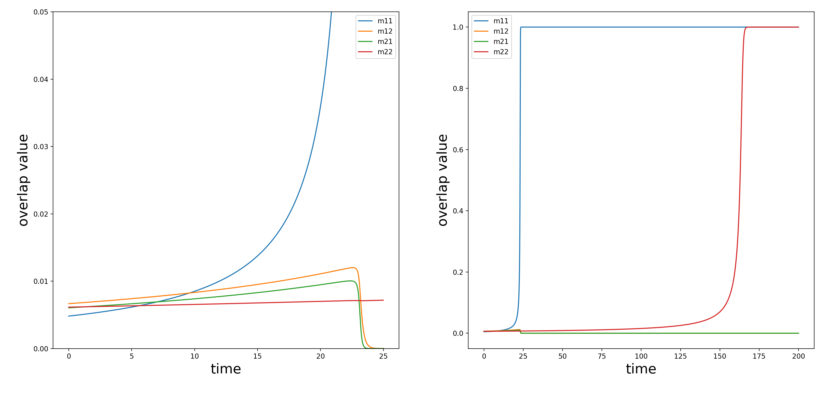
Figure 1. Evolution of the correlations $m_{ij}$ under the population dynamics in the case where $p=3$, $r=2$, $\lambda_{1}=3$ and $\lambda_{2}=1$. The SNRs are sufficiently separated to ensure exact recovery of both spikes $\boldsymbol{v}_{1}$ and $\boldsymbol{v}_{2}$. Once $m_{11}$ reaches a sufficiently large microscopic threshold, $m_{12}$ and $m_{21}$ begin to decrease. Recovery of $\boldsymbol{v}_{2}$ is then possible after $m_{12}$ and $m_{21}$ have decreased sufficiently, becoming negligible in the evolution of $m_{22}$.

The dynamics underlying Theorems 1.3 and 1.5 reveals a richer structure beyond the stated results. In particular, the correlation $m_{i_{1}^{\ast}j_{1}^{\ast}}$ becomes macroscopic first, followed by $m_{i_{2}^{\ast}j_{2}^{\ast}}$, and so on. Theorem 1.3 involves an additional assumption on the ratio between the signal sizes, which ensures that variations due to random initialization are mitigated by differences in the SNRs. As a result, the greedy maximum selection of $\boldsymbol{I}_{0}$ results in $i_{k}^{\ast}=j_{k}^{\ast}=k$ for every $k\in[r]$, allowing $m_{11},\ldots,m_{rr}$ to become macroscopic in sequence. More precisely, as shown by the numerical simulations in Figures 1,  2 and 6, when $m_{i_{1}^{\ast}j_{1}^{\ast}}$ exceeds a critical microscopic threshold (which depends on the order $p$ of the tensor and on the SNRs), the correlations $m_{i_{1}^{\ast}j}$ and $m_{ij_{1}^{\ast}}$ for $i\neq i_{1}^{\ast},j\neq j_{1}^{\ast}$ decrease to sufficiently small levels. This allows $m_{i_{2}^{\ast}j_{2}^{\ast}}$ to grow and become macroscopic, and the process continues similarly for the remaining correlations $m_{i_{k}^{\ast}j_{k}^{\ast}}$. This phenomenon is referred to as the sequential elimination process: the correlations $\{m_{i_{k}^{\ast}j_{k}^{\ast}}\}_{k=1}^{r}$ increase one by one, sequentially eliminating correlations that share a row or column index. This is formalized as follows.

Definition 1.6 (Sequential elimination).

Let $S=\{(i_{1},j_{1}),\ldots,(i_{r},j_{r})\}$ be a set with distinct $i_{1},\ldots,i_{r}\in[r]$ and distinct $j_{1},\ldots,j_{r}\in[r]$. We say that the correlations $\{m_{ij}(t)\}_{1\leq i,j\leq r}$ follow a sequential elimination with ordering $S$ if there exist $r$ stopping times $T_{1}\leq\cdots\leq T_{r}$ such that for every $k\in[r]$, every $\varepsilon,\varepsilon^{\prime}>0$, and every $T\geq T_{k}$,

$$|m_{i_{k}j_{k}}(\boldsymbol{X}_{T})|\geq 1-\varepsilon\quad\textnormal{and}\quad|m_{i_{k}j}(\boldsymbol{X}_{T})|\leq\varepsilon^{\prime},|m_{ij_{k}}(\boldsymbol{X}_{T})|\leq\varepsilon^{\prime}\enspace\textnormal{for}\>i\neq i_{k},j\neq j_{k}.$$

Based on Definition 1.6, we have the following result, which serves as a foundation for Theorem 1.5.

Theorem 1.7 (Theorem 1.5 revisited).

Let $(\boldsymbol{X}_{\ell})_{\ell\in\mathbb{N}}$ be online SGD initialized from $\boldsymbol{X}_{0}\sim\mu_{N\times r}$ with step-size $\delta\ll\log(N)^{-1}N^{-\frac{p-3}{2}}$. Let $M\gg\log(N)N^{p-2}$. Then, the correlations $\{m_{ij}\}_{1\leq i,j\leq r}$ follow a sequential elimination with ordering $\{(i_{k}^{\ast},j_{k}^{\ast})\}_{k=1}^{r}$ and stopping times of order $\log(N)N^{p-2}$, with $\mathbb{P}$-probability $1$ in the large-$N$ limit.

We can formulate an analogous version of Theorem 1.7 for Theorem 1.3 by adding the corresponding assumption on the ratio between the SNRs.

Remark 1.8.

It is important to note that in the above results, namely Theorems 1.3, 1.5 and 1.7, the behavior of online SGD depends on the parity of $p$ in the following sense. When $p$ is odd, then each estimator $\boldsymbol{x}_{j_{k}^{\ast}}$ recovers the spike $\boldsymbol{v}_{i_{k}^{\ast}}$ with $\mathbb{P}$-probability $1-o(1)$, since the correlations that are negative at initialization get trapped at the equator. Conversely, when $p$ is even, we have that each estimator $\boldsymbol{x}_{j_{k}^{\ast}}$ recovers $\textnormal{sgn}(m_{i_{k}^{\ast}j_{k}^{\ast}}(\boldsymbol{X}_{0}))\boldsymbol{v}_{i_{k}^{\ast}j_{k}^{\ast}}$ with probability $1-o(1)$. This means that if the correlation at initialization is positive, then $\boldsymbol{x}_{j_{k}^{\ast}}$ recovers $\boldsymbol{v}_{i_{k}^{\ast}}$; otherwise, $\boldsymbol{x}_{j_{k}^{\ast}}$ recovers $-\boldsymbol{v}_{i_{k}^{\ast}}$.

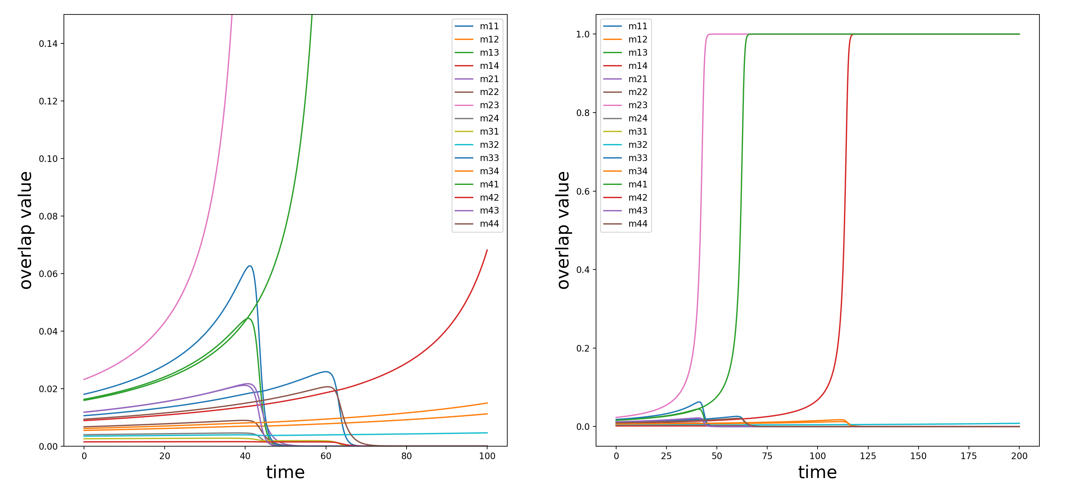
Figure 2. Evolution of the correlations $m_{ij}$ under the population dynamics in the case where $p=3$, $r=4$, $\lambda_{1}=\cdots=\lambda_{4}=1$. Since the SNRs are all equal, the order in which the correlations become macroscopic is determined by the values of the correlations at initialization, see Definition 1.4. This numerical simulation shows the recovery of a permutation of the four spikes $\boldsymbol{v}_{1},\ldots,\boldsymbol{v}_{4}$ according to the sequential elimination phenomenon.

1.2.2. Main results for $p=2$

We now present our main results for $p=2$. Our first result shows that exact recovery of all spikes is possible, provided sufficiently separated SNRs and a sample complexity of order $\log(N)^{2}N^{\frac{\xi}{2}}$, where $\xi\in(0,1)$ depends on the relative sizes of the signals.

Theorem 1.9 (Exact recovery for $p=2$).

Let $(\boldsymbol{X}_{\ell})_{\ell\in\mathbb{N}}$ be online SGD initialized from $\boldsymbol{X}_{0}\sim\mu_{N\times r}$ with step-size $\delta\ll\frac{1}{\log(N)}N^{\frac{1}{2}\frac{\lambda_{r}^{2}}{\lambda_{1}^{2}}}$. Let $M\gg\log(N)^{2}N^{\frac{1}{2}\left(1-\frac{\lambda_{r}^{2}}{\lambda_{1}^{2}}\right)}$. Assume that $\lambda_{i}=\lambda_{i+1}(1+\kappa_{i})$ for every $1\leq i\leq r-1$, with $\kappa_{i}>0$ being constants of order $1$. Then, for every $\varepsilon>0$ and every $i\in[r]$,

$$\lim_{N\to\infty}\mathbb{P}_{\boldsymbol{X}_{0}}\left(\lvert m_{ii}(\boldsymbol{X}_{M})\rvert\geq 1-\varepsilon\right)=1.$$

Similar to Theorem 1.3, variations in the correlations at initialization are compensated by differences in SNRs, leading to exact recovery of all spikes. However, unlike Theorem 1.3, for $p=2$, exact recovery is achievable as soon as the SNRs differ by factors of order $1$. In terms of sample complexity, there is a significant difference compared to the result obtained in [10] for the rank-one matrix PCA problem, where a number of $\log(N)^{2}$ samples is sufficient for efficiently recovering the spike. In our case, this sample complexity threshold is not sufficient to ensure the stability of the evolution of the subsequent correlations. The difference between both thresholds arises from the control of the retraction map, which is inherent to the online SGD algorithm on the Stiefel manifold. This is illustrated in the numerical simulation shown in Figure 8, and the term responsible for this discrepancy is rigorously quantified in the proof of Lemma 5.5.

As with the case of $p\geq 3$, the correlations exhibit a sequential elimination with ordering $\{(k,k)\colon k\in[r]\}$. Thus, an analogous version of Theorem 1.7 can be stated for Theorem 1.9. The evolution of the correlations is illustrated by the numerical simulations shown in Figures 3 and 4. As noted in Remark 1.8, the behavior of online SGD depends on the parity of the order $p$ of the tensor. Specifically, for $p=2$, the recovery of the unknown vector $\boldsymbol{v}_{i}$ or its negative counterpart $-\boldsymbol{v}_{i}$ is determined by the sign of the correlation $m_{ii}$ at initialization.

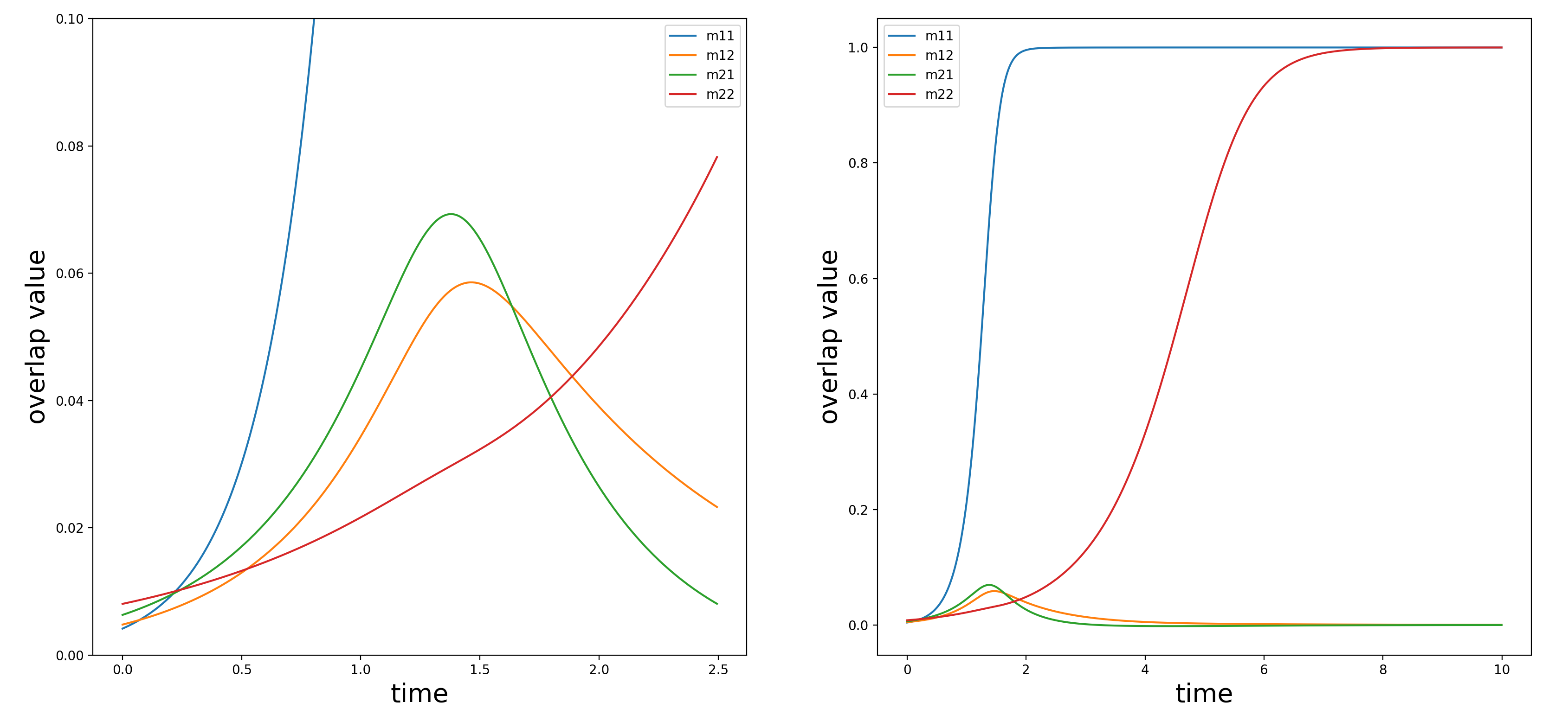
Figure 3. Evolution of the correlations $m_{ij}$ under the population dynamics in the case where $p=2$, $r=2$, $\lambda_{1}=3$ and $\lambda_{2}=1$. The SNRs are sufficiently separated to ensure exact recovery of both spikes, following the elimination of $m_{12},m_{21}$ by $m_{11}$.

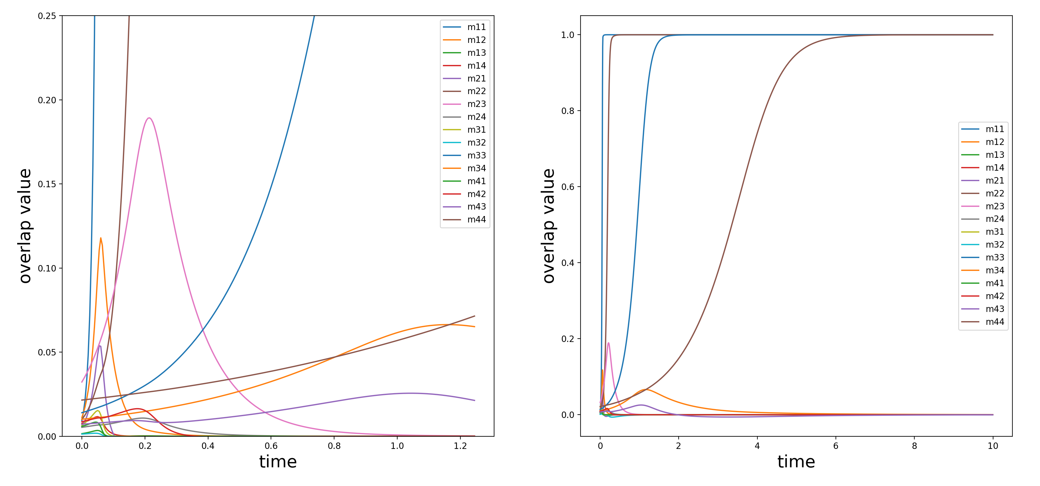
Figure 4. Evolution of the correlations $m_{ij}$ under the population dynamics in the case where $p=2$, $r=4$, $\lambda_{1}=10,\lambda_{2}=5,\lambda_{3}=2$ and $\lambda_{1}=1$. We observe a sequential elimination phenomenon, although less pronounced than in the case $p\geq 3$, in the sense that correlations that eventually become negligible can still exhibit significant increases.

Our second main result for $p=2$ addresses the case where the SNRs are all equal. Due to the invariance of the loss function $\mathcal{L}_{N,r}$ under both right and left rotations, our focus shifts from recovering each individual signal to recovering the subspace spanned by the signal vectors $\boldsymbol{v}_{1},\ldots,\boldsymbol{v}_{r}$. This notion of recovery is referred to as subspace recovery and is defined as follows.

Definition 1.10 (Subspace recovery).

We say that we recover the subspace spanned by the orthogonal signal vectors $\boldsymbol{v}_{1},\ldots,\boldsymbol{v}_{r}$ if

$$\lVert\boldsymbol{X}\boldsymbol{X}^{\top}-\boldsymbol{V}\boldsymbol{V}^{\top}\rVert_{\textnormal{F}}=o(1),$$

with high probability, where $\lVert\cdot\rVert_{\textnormal{F}}$ stands for the Frobenius norm and $\boldsymbol{X}=[\boldsymbol{x}_{1},\ldots,\boldsymbol{x}_{r}],\boldsymbol{V}=[\boldsymbol{v}_{1},\ldots,\boldsymbol{v}_{r}]\in\mathbb{R}^{N\times r}$.

From Definition 1.10, we note that subspace recovery is equivalent to recovering the eigenvalues of the matrix $\boldsymbol{G}\in\mathbb{R}^{r\times r}$ defined by

$$\boldsymbol{G}=\boldsymbol{M}\boldsymbol{M}^{\top},\quad\textnormal{with}\quad\boldsymbol{M}=\boldsymbol{V}^{\top}\boldsymbol{X}=(m_{ij}(\boldsymbol{X}))_{1\leq i,j\leq r}\in\mathbb{R}^{r\times r},$$

since it holds that $\lVert\boldsymbol{X}\boldsymbol{X}^{\top}-\boldsymbol{V}\boldsymbol{V}^{\top}\rVert_{\textnormal{F}}=2(r-\operatorname{Tr}(\boldsymbol{G}))$. Hereafter, we let $\theta_{1}(\boldsymbol{X}),\ldots,\theta_{r}(\boldsymbol{X})$ denote the eigenvalues of the matrix-valued function $\boldsymbol{G}(\boldsymbol{X})$. Our main result is as follows.

Theorem 1.11 (Subspace recovery for $p=2$).

Let $\lambda_{1}=\cdots=\lambda_{r}$. Let $(\boldsymbol{X}_{\ell})_{\ell\in\mathbb{N}}$ be online SGD initialized from $\boldsymbol{X}_{0}\sim\mu_{N\times r}$ with step-size $\delta\ll\frac{1}{\log(N)^{2}}N^{\frac{1}{2}}$. Let $M\gg\log(N)^{3}$. Then, for every $\varepsilon>0$ and $i\in[r]$,

$$\lim_{N\to\infty}\mathbb{P}_{\boldsymbol{X}_{0}}\left(\theta_{i}(\boldsymbol{X}_{M})\geq 1-\varepsilon\right)=1.$$

The recovery dynamics in this case differs significantly from those in the previous cases: the correlations evolve at similar rates, thereby preventing the sequential elimination phenomenon, as shown in the left-hand side of Figure 5. However, as illustrated on the right-hand side of Figure 5, the eigenvalues of $\boldsymbol{G}$ establish a natural ordering at initialization, which persists throughout their evolution until recovery, resulting in a monotone evolution.

Unlike the tensor case, where we analyze the dynamics for any value of the signal sizes, for $p=2$ we have focused on two cases: when the parameters are separated by constants of order $1$ (i.e., Theorem 1.9) and when they are all equal (i.e., Theorem 1.11). The intermediate case, where the SNRs are separated by a sufficiently small $\epsilon$-factor, possibly depending on $N$, requires further effort and will be addressed in future work.

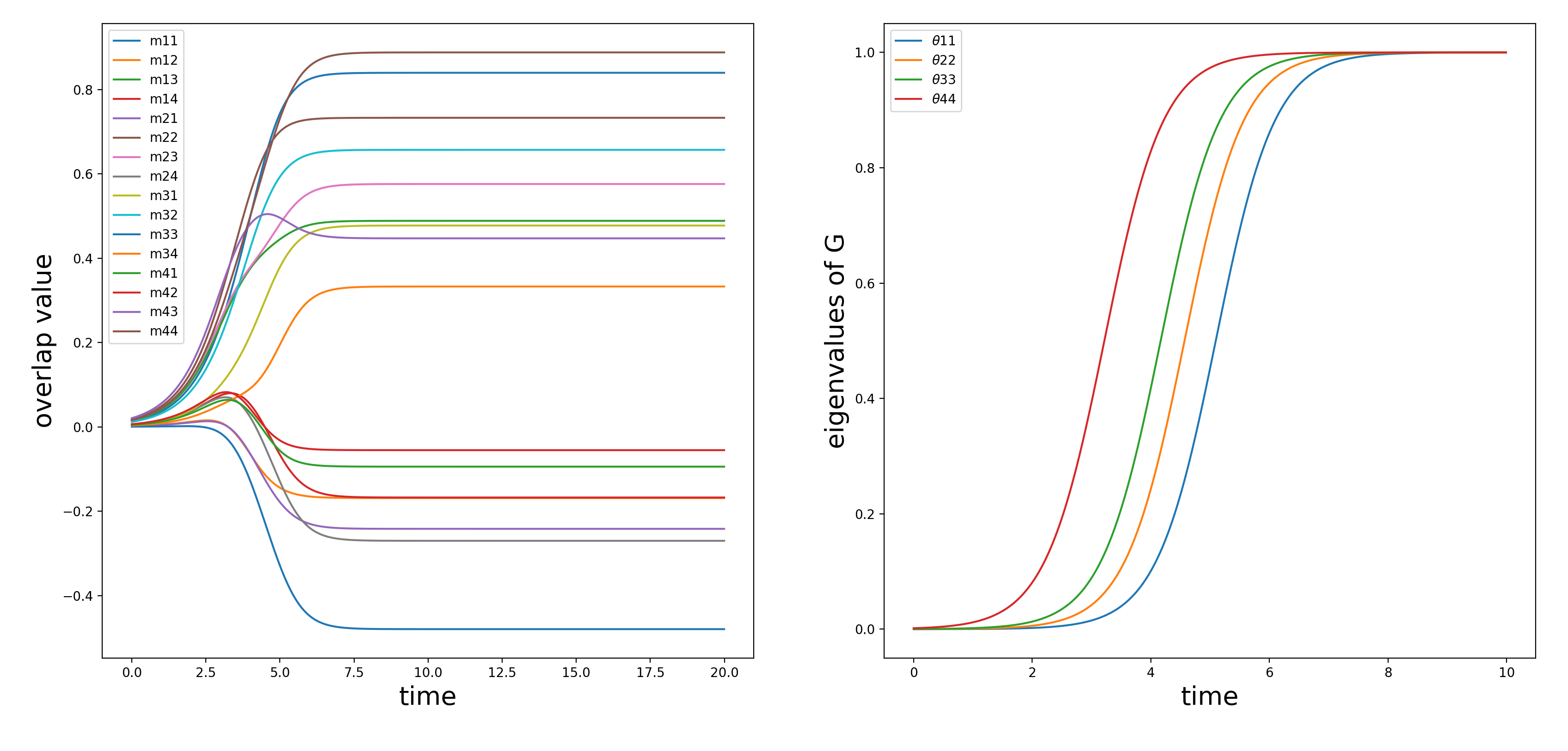
Figure 5. Evolution of the correlations $m_{ij}$ (left) and eigenvalues (right) of $\boldsymbol{G}=\boldsymbol{M}\boldsymbol{M}^{\top}$ under the population dynamics. The relative speeds of the correlations are too close to each other for a sequential elimination phenomenon to take place. However, the eigenvalues of $\boldsymbol{G}$ are monotone and it is possible to characterize subspace recovery.

We conclude this section by presenting simulations of the high-dimensional online SGD algorithm in the case with three hidden directions. We refer to Figure 6 for the case where $p=3$ and to Figure 7 for the case where $p=2$. Additionally, Figure 8 illustrates the numerical instability observed for $p=2$ due to the retraction map, as discussed in the paragraph following Theorem 1.9.

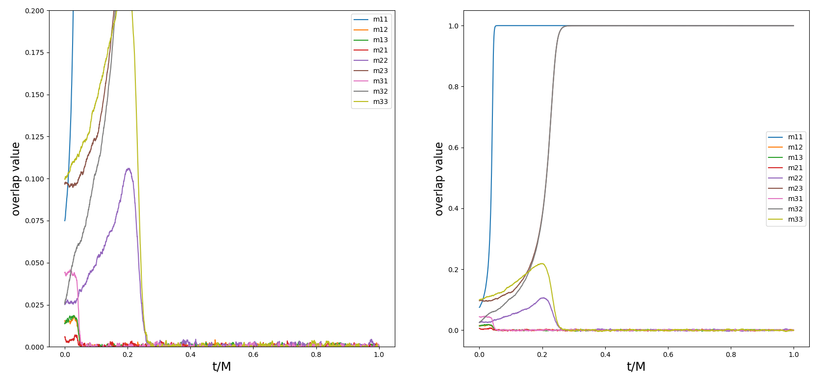
Figure 6. Evolution of the correlations $m_{ij}$ under the online SGD algorithm for the case where $p=3,r=3$, with SNRs $\lambda_{1}=3,\lambda_{2}=2,\lambda_{3}=1$. The simulation is performed with $M=3200$ samples, a step-size $\delta/N=0.0003$, and a dimension of $N=500$. The simulation shows recovery of a permutation of the spikes.

Figure 7. Evolution of the correlations $m_{ij}$ under the online SGD algorithm for the case where $p=2,r=3$, with SNRs $\lambda_{1}=3,\lambda_{2}=2,\lambda_{3}=1$. The simulation is performed with $M=230$ samples, a step-size $\delta/N=0.002$, and a dimension of $N=500$. The simulation shows exact recovery of the spikes.

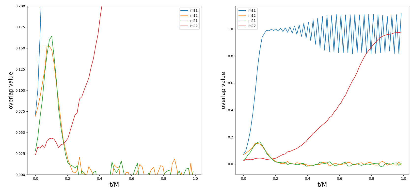
Figure 8. Evolution of the correlations $m_{ij}$ under the online SGD algorithm for the case where $p=2,r=2$, with SNRs $\lambda_{1}=2,\lambda_{2}=1$. The simulation is performed with $M=70$ samples, a step-size $\delta/N=0.006$, and a dimension of $N=500$. While the correlations $m_{11}$ and $m_{22}$ clearly overcome the effect of the noise martingale and become macroscopic, the algorithm becomes unstable. This illustrates the fact that the sample complexity prescribed by Theorem 1.9 is larger than what is required to just ensure that the martingale term is negligible compared to the signal drift.

1.3. Related works

We now provide a detailed overview on detection and recovery thresholds within the spiked tensor model, along with a discussion of main results for multi-index models.

Montanari and Richard [53] conjectured that for the single-spiked model, local algorithms with random initialization require a sample complexity scaling as $N^{p-2}$ to efficiently recover the unknown spike, while a sharper threshold scaling as $N^{\frac{p-2}{2}}$ is sufficient using Sum-of-Squares (SoS) and spectral methods. The computational threshold $N^{p-2}$ was achieved using various local methods: gradient flow and Langevin dynamics [9], online SGD [10], and tensor power iteration [37, 67]. For local algorithms, the order $p$ of the tensor determines the curvature of the landscape near the initial condition, which influences the recovery difficulty. The sharp threshold of $N^{\frac{p-2}{2}}$ was achieved using SoS-based algorithms [36, 35, 40], spectral methods based on the Kikuchi Hessian [66], and tensor unfolding [13]. Beyond computational thresholds for efficiently estimating the unknown direction, significant research has focused on two other critical thresholds: the information-theoretic threshold for detection of the signal [43, 52, 51, 22, 38, 5], and the statistical threshold validating MLE as a reliable statistical method [14, 55, 38]. Detection and recovery thresholds for the multi-rank tensor PCA model have also been explored. On the information-theoretic side, it has been shown in [42] for $p=2$ and in [23] for $p\geq 3$ that there is an order-$1$ critical threshold for the SNRs, above which it is possible to detect the unseen low-rank signal tensor $\sqrt{N}\sum_{i=1}^{r}\lambda_{i}\boldsymbol{v}_{i}^{\otimes p}$. On the algorithmic side, [37] studied the power iteration algorithm and determined the local threshold for efficiently recovering the finite-rank signal component. In the extended version of our preprint [6], we studied Langevin and gradient flow dynamics for the multi-spiked tensor PCA. We demonstrated that the sample complexity required to efficiently recover all spikes scales as $N^{p-1}$ for $p\geq 3$, while for $p=2$ as $N^{1+\delta-\lambda_{r}^{2}/\lambda_{1}^{2}}$ for every $\delta>0$ not depending on $N$. These thresholds are suboptimal compared to those obtained here using online SGD due to challenges involved by controlling the noise generator under Langevin and gradient flow dynamics.

As mentioned earlier at the beginning of this section, the single/multi-spiked tensor model belongs to the broader class of single/multi-index models. In the context of single-index models, when the hidden link function $\sigma^{\ast}$ is known, the behavior of online SGD exhibits similar phenomenology to the single-spiked tensor PCA model [10]. On the other hand, when the hidden link function $\sigma^{\ast}$ is unknown, recent works by Bietti, Bruna, and Sanford [17], as well as by Berthier, Montanari, and Zhou [15], have studied the ability of two-layer neural networks to jointly learn the hidden link function and the hidden vector. They achieved this using various instances of gradient flow, either coupled with non-parametric regression steps or by employing a separation of timescales between the inner and outer layers. In the context of multi-index models, several recent works have provided upper bounds on the sample complexity thresholds required for shallow neural networks trained with first-order optimization methods to learn multi-index models. For instance, [46, 25, 3] analyzed the benefits given by a single gradient step coupled with various choices for the second layer weights. Although these works determine the sample complexity required for the gradient to achieve macroscopic correlation with the target subspace and illustrate how neural networks improve over kernel methods, they offer limited insight into the global convergence when training the first layer weights. Using an online layer-wise training approach and regression steps on the second layer weights, Abbe, Boix-Adsera, and Misiakiewicz [2] introduced generalizations of the information exponent from [10] for multi-index functions, referred to as the leap-exponent, and proved that their dynamics successively visits several saddle-points before recovering the unknown subspace. A similar analysis was carried out by Dandi et al. [26], providing further sample complexity guarantees when using large batches of data over a few gradient steps. Moreover, Bietti, Bruna, and Pillaud-Vivien studied in [16] the population, continuous time limit of a two step procedure, where each gradient step on the estimator of the hidden subspace is coupled with a multivariate non-parametric regression step to estimate the link function. They showed that this two-step procedure makes the landscape benign, leading to the recovery of both the hidden link function and the correct subspace after saddle-to-saddle dynamics similar to the one exhibited in [2]. These works extensively rely on the separation of timescales and regression steps, resulting in a superposition of monotone dynamics, allowing for generality at the level of the link function while focusing on subspace recovery. In contrast, our work provides a complete description of the dynamics for online SGD in the context of a specific multi-index model, yielding recovery of permutations and rotations (when $p=2$ and the SNRs are equal).

In the field of statistical physics of learning and the related results in high-dimensional probability, single- and multi-index models can be viewed as examples of the teacher-student model, see e.g. [29, 71], in which a specific target function is learned using a chosen architecture, typically with knowledge of the form of the hidden model. The dynamics of gradient-based methods are usually studied using closed-form, low-dimensional, and asymptotically exact dynamical systems towards which the gradient trajectories are shown to concentrate as the input dimension and number of sample diverge while remaining proportional. In the case of online learning, these dynamics lead to sets of ordinary differential equations (ODEs). For instance, such ODEs have been analyzed for committee machines [56] and two-layer neural networks [34, 63]. When a full-batch is used, the correlations throughout the entire trajectory result in a set of integro-differential equations, known as dynamical mean-field theory in statistical physics, for which there has been renewed interest in recent years in the context of classification problems and learning single and multi-index functions in the proportional limit of dimension and number of samples, using both powerful heuristics [57, 58, 45], and rigorous methods  [21, 33]. Despite their theoretical significance, the resulting equations are often challenging to analyze beyond a few steps and are limited to studying linear sample complexity regimes. As a consequence, applying these tools to address questions related to global convergence, characterization of fixed points, or achieving polynomial sample complexity remains difficult.

Finally, the limiting dynamics of online SGD has recently been studied in [11, 12, 7] for broad range of estimation and classification tasks, including learning an XOR function using a two-layer neural network. In particular, [11, 12] shows the existence of critical regimes in the step-size that lead to an additional term in the population dynamics, referred to as the corrector, which also appears in the statistical physics literature, e.g. [56, 34]. By appropriately rescaling the step size, they also obtain diffusive limits for online SGD. In [7], a spectral analysis is performed to study the evolution of the Hessian of the loss landscape, showing alignment of the SGD trajectories with emerging eigenspaces. We defer the exploration of critical step sizes, diffusive limits, and spectral phenomena to future work, focusing here on obtaining non-asymptotic results and enhancing our understanding of the population dynamics.

1.4. Overview

An overview of the paper is given as follows. Section 2 provides an outline of the proofs of our main results. In Section 3, we present the nonasymptotic versions of our main results, from which we derive the main asymptotic results of Subsection 1.2. Sections 4-6 are devoted to the proofs of the main results in their nonasymptotic form. Specifically, Section 4 presents comparison inequalities for both the correlations $m_{ij}(\boldsymbol{X})$ and the eigenvalues of $\boldsymbol{M}\boldsymbol{M}^{\top}$ with $\boldsymbol{M}=(m_{ij}(\boldsymbol{X}))_{i,j\in[r]}$. Section 5 provides the proofs of the main results related to the full recovery of the spikes, i.e., it addresses the case where $p\geq 3$ with arbitrary values for the SNRs, as well as the case where $p=2$ with sufficiently separated SNRs. Finally, Section 6 focuses on the case where $p=2$ and the spikes have equal SNRs, thereby proving subspace recovery.

Acknowledgements. G.B. and C.G. acknowledge the support of the NSF grant DMS-2134216. V.P. acknowledges the support of the ERC Advanced Grant LDRaM No. 884584.

2. Outline of proofs

In this section, we outline the proofs of our main results. To simplify the discussion, we focus on the spiked tensor model with $r=2$. First, we address the cases where $p\geq 3$ with arbitrary values of $\lambda_{1}$ and $\lambda_{2}$, as well as the case where $p=2$ with sufficiently separated SNRs. In these cases, we follow the evolution of the correlations under the online SGD algorithm and show full recovery of the spikes. Next, we consider the case where $p=2$ and the spikes have equal strength, i.e., $\lambda_{1}=\lambda_{2}$, and show that the algorithm recovers the subspace spanned by the two spikes.

2.1. Full recovery of spikes

We begin by analyzing the evolution of the correlations $m_{ij}$ under the online SGD algorithm, following the update rule given by (1.6). We assume an initial random start with a completely uninformative prior, specifically the invariant distribution on the Stiefel manifold. As a consequence, all correlations $m_{ij}$ have the typical scale of order $N^{-\frac{1}{2}}$ at initialization. For simplicity, we assume that all correlations are positive at initialization.

According to (1.6), the evolution equation for the correlations $m_{ij}(\boldsymbol{X}_{t})$ at time $t$ is given by

$$m_{ij}(\boldsymbol{X}_{t})=\left\langle\boldsymbol{v}_{i},R_{\boldsymbol{X}_{t-1}}\left(-\frac{\delta}{N}(\nabla_{\textnormal{St}}\mathcal{L}_{N,r}(\boldsymbol{X}_{t-1};\boldsymbol{Y}^{t}))_{j}\right)\right\rangle.$$

To simplify notation, we write $m_{ij}(t)=m_{ij}(\boldsymbol{X}_{t})$. When the step-size $\delta>0$ is sufficiently small, the matrix inverse in the polar retraction term $R_{\boldsymbol{X}_{t-1}}$ (see (1.7)) can be expanded as a Neumann series. Thus, up to controlled error terms, we have that

$$m_{ij}(t)\approx m_{ij}(t-1)-\langle\boldsymbol{v}_{i},\frac{\delta}{N}(\nabla_{\textnormal{St}}\mathcal{L}_{N,r}(\boldsymbol{X}_{t-1};\boldsymbol{Y}^{t}))_{j}\rangle.$$

Iterating this expression yields

$$m_{ij}(t)\approx m_{ij}(0)-\frac{\delta}{N}\sum_{\ell=1}^{t}\langle\boldsymbol{v}_{i},(\nabla_{\textnormal{St}}\mathcal{L}_{N,r}(\boldsymbol{X}_{\ell-1}))_{j}\rangle.$$ (2.1)

The condition on the step-size $\delta$ required for the Neumann series to converge is not restrictive and does not present a bottleneck in our proof. However, the retraction map introduces additional interaction terms among the correlations, which demand a careful analysis.

Having the evolution equations for the correlations at hand, we decompose the gradient of the loss function $\mathcal{L}_{N,r}$ into noise and population components, i.e.,

$$\nabla_{\textnormal{St}}\mathcal{L}_{N,r}(\boldsymbol{X}_{t-1},\boldsymbol{Y}^{t})=\nabla_{\textnormal{St}}H_{N,r}(\boldsymbol{X}_{t-1})+\nabla_{\textnormal{St}}\Phi_{N,r}(\boldsymbol{X}_{t-1}),$$

where $H_{N,r}$ and $\Phi_{N,r}$ are given by (1.4) and (1.5), respectively. By balancing these two terms, we determine the sample complexity thresholds for efficient recovery. Following the approach used to prove [10, Proposition 4.1], we control the magnitude of the noise part by appropriately adjusting the step-size $\delta$, ensuring the signal term dominates over a sufficiently large time scale for efficient recovery. However, unlike the single-spiked case in [10, Proposition 4.1], the contribution from the population loss leads to a significantly more complicated dynamics, requiring careful analysis to control the nonmonotonic interactions among the correlations. At the same time, our control needs to be sufficiently sharp to meet sample complexities and discretization guarantees that are statistically and algorithmically relevant.

2.1.1. Control of the noise term

The evolution equation (2.1) can be rewritten as

$$m_{ij}(t)\approx m_{ij}(0)-\frac{\delta}{N}\sum_{\ell=1}^{t}\langle\boldsymbol{v}_{i},(\nabla_{\textnormal{St}}\Phi_{N,r}(\boldsymbol{X}_{\ell-1}))_{j}\rangle-\frac{\delta}{N}\sum_{\ell=1}^{t}\langle\boldsymbol{v}_{i},(\nabla_{\textnormal{St}}H_{N,r}(\boldsymbol{X}_{\ell-1}))_{j}\rangle,$$

where a simple computation shows that

$$\begin{split}-\langle\boldsymbol{v}_{i},(\nabla_{\textnormal{St}}\Phi_{N,r}(t))_{j}\rangle&=p\sqrt{N}\lambda_{i}\lambda_{j}m_{ij}^{p-1}(t)\\ &\quad-\frac{p}{2}\sqrt{N}\sum_{1\leq k,\ell\leq 2}\lambda_{k}m_{i\ell}(t)m_{kj}(t)m_{k\ell}(t)\left(\lambda_{j}m_{kj}^{p-2}(t)+\lambda_{\ell}m_{k\ell}^{p-2}(t)\right).\end{split}$$

The noise term corresponds to the sum of the martingale increments $-\langle\boldsymbol{v}_{i},(\nabla_{\textnormal{St}}H_{N,r}(\boldsymbol{X}_{\ell-1}))_{j}\rangle$, and since the noise tensors $(\boldsymbol{W}^{\ell})_{\ell}$ are sub-Gaussian, classical concentration inequalities for the sub-Gaussian distribution can be applied to bound this term. The population part consists of two terms: a drift term $p\sqrt{N}\lambda_{i}\lambda_{j}m_{ij}^{p-1}$ which dominates the dynamics, particularly near initialization, and a correction term $\frac{p}{2}\sqrt{N}\sum_{1\leq k,\ell\leq r}\lambda_{k}m_{i\ell}m_{kj}m_{k\ell}\left(\lambda_{j}m_{kj}^{p-2}+\lambda_{\ell}m_{k\ell}^{p-2}\right)$ which arises due to the constraint of the estimator $\boldsymbol{X}$ being on an orthogonal manifold. For the correlation $m_{ij}$ to increase, the drift term needs to be larger than both the noise and correction terms. Near initialization, the correlations typically scale as $N^{-\frac{1}{2}}$ and the drift term dominates the correction term. Moreover, near initialization, the noise term can be absorbed by $m_{ij}(0)$. This gives that

$$m_{ij}(t)\approx m_{ij}(0)+\frac{\delta}{\sqrt{N}}p\lambda_{i}\lambda_{j}\sum_{\ell=1}^{t}m_{ij}^{p-1}(\ell-1).$$ (2.2)

At this point, we need to show that the drift term continues to dominate the noise term over a sufficiently long time scale, allowing the correlations $m_{ij}$ to escape mediocrity. Once the first correlation reaches a critical threshold, the previously negligible correction term in the population loss becomes significant, and the dynamics shifts to a more delicate phase where the correlations begin to interact with one another, as explained below.

2.1.2. Analysis of the population dynamics

We now analyze the evolution of the correlations by studying the population dynamics, first for the case $p\geq 3$, and then for $p=2$.

Recovery for $p\geq 3$. The solution of (2.2) is given by

$$m_{ij}(t)\approx m_{ij}(0)\left(1-\frac{\delta}{\sqrt{N}}p\lambda_{i}\lambda_{j}m_{ij}(0)^{p-2}t\right)^{-\frac{1}{p-2}},$$ (2.3)

where $m_{ij}(0)=\frac{\gamma_{ij}}{\sqrt{N}}$. The typical time for $m_{ij}$ to reach a macroscopic threshold $\varepsilon>0$, denoted by $T_{\varepsilon}^{(ij)}$, is therefore given by

$$T_{\varepsilon}^{(ij)}\approx\frac{1-\left(\frac{\gamma_{ij}}{\varepsilon\sqrt{N}}\right)^{p-2}}{\delta\lambda_{i}\lambda_{j}p\gamma_{ij}^{p-2}}N^{\frac{p-2}{2}}.$$

In particular, the first correlation to become macroscopic is the one associated with the largest value of $\lambda_{i}\lambda_{j}\gamma_{ij}^{p-2}$, where $(\gamma_{ij})_{1\leq i,j\leq 2}$ approximately follow independent standard normal distributions. According to Definition 1.4, this corresponds to the pair $(i_{1}^{\ast},j_{1}^{\ast})$ of the greedy maximum selection of the matrix $\boldsymbol{I}_{0}=(\lambda_{i}\lambda_{j}m_{ij}(0)^{p-2}\mathbf{1}_{\{m_{ij}^{p-2}(0)\geq 0\}})_{ij}$. Once the first correlation $m_{ij}$ reaches a macroscopic value $\varepsilon>0$, the other correlations are still trapped near the equator. This can be verified by plugging the value of $T_{\varepsilon}^{(i_{1}^{\ast}j_{1}^{\ast})}$ into (2.3). Note that if the SNRs are sufficiently separated to compensate for initialization differences, with high probability, $m_{11}$ is the first correlation to escape mediocrity. In the following, without loss of generality we may assume that $i_{1}^{\ast}=j_{1}^{\ast}=1$, i.e., $m_{11}$ is the first correlation to reach the macroscopic threshold $\varepsilon$.

Next, we describe the evolution of $m_{12},m_{21}$ and $m_{22}$ as $t\geq T_{\varepsilon}^{(11)}$. We first note that the correction part of the population term, i.e.,

$$\sum_{1\leq k,\ell\leq 2}\lambda_{k}m_{kj}(t)m_{k\ell}(t)m_{i\ell}(t)(\lambda_{j}m_{kj}^{p-2}(t)+\lambda_{\ell}m_{k\ell}^{p-2}(t)),$$

becomes dominant in the evolution of the correlations $m_{12},m_{21}$, as soon as $m_{11}$ reaches the microscopic threshold $N^{-{\frac{p-2}{2p}}}$. In other words, $m_{12}$ and $m_{21}$ are non-decreasing and they begin to decrease as soon as $m_{11}$ reaches this microsopic threhsold. On the other hand, the correction part of the population generator may become dominant in the evolution of $m_{22}$, as soon as $m_{11}$ reaches another microscopic threshold of order $N^{-{\frac{p-3}{2(p-1)}}}$, leading to a potential decrease of $m_{22}$. Through a careful analysis, we show that this potential decrease is at most of order $\frac{\log(N)}{N}$, so that $m_{22}$ remains stable at the scale $\frac{1}{\sqrt{N}}$ during the ascending phase of $m_{11}$. The evolution of the correlations $m_{12},m_{21}$ and $m_{22}$ as $m_{11}$ becomes macroscopic is illustrated by the numerical experiment in Figure 9. Once $m_{12},m_{21}$ become sufficiently small, we show that the evolution of $m_{22}$ can still be described by (2.3), thus ensuring the recovery of the second direction. The phenomenon we observe here is referred to as sequential elimination phenomenon, as introduced in Definition 1.6. The correlations increase sequentially, one after another. When a correlation (e.g., $m_{11}$) exceeds a certain threshold, the correlations sharing a row and column index (e.g., $m_{12},m_{21}$) start decreasing until they become sufficiently small to be negligible, thereby enabling the subsequent correlations (e.g., $m_{22}$) to increase. This phenomenon is illustrated in Figure 1. We remark that if the SNRs are sufficiently separated as described earlier, then exact recovery of the unknown signal vectors is achieved with high probability, which depends on the ratio between the signal sizes, as stated in Theorem 1.3. Otherwise, recovery results in a permutation of the spikes, determined by the greedy maximum selection of the matrix $\boldsymbol{I}_{0}=(\lambda_{i}\lambda_{j}m_{ij}(0)^{p-2}\mathbf{1}_{\{m_{ij}^{p-2}(0)\geq 0\}})_{ij}$, as illustrated in Figure 2.

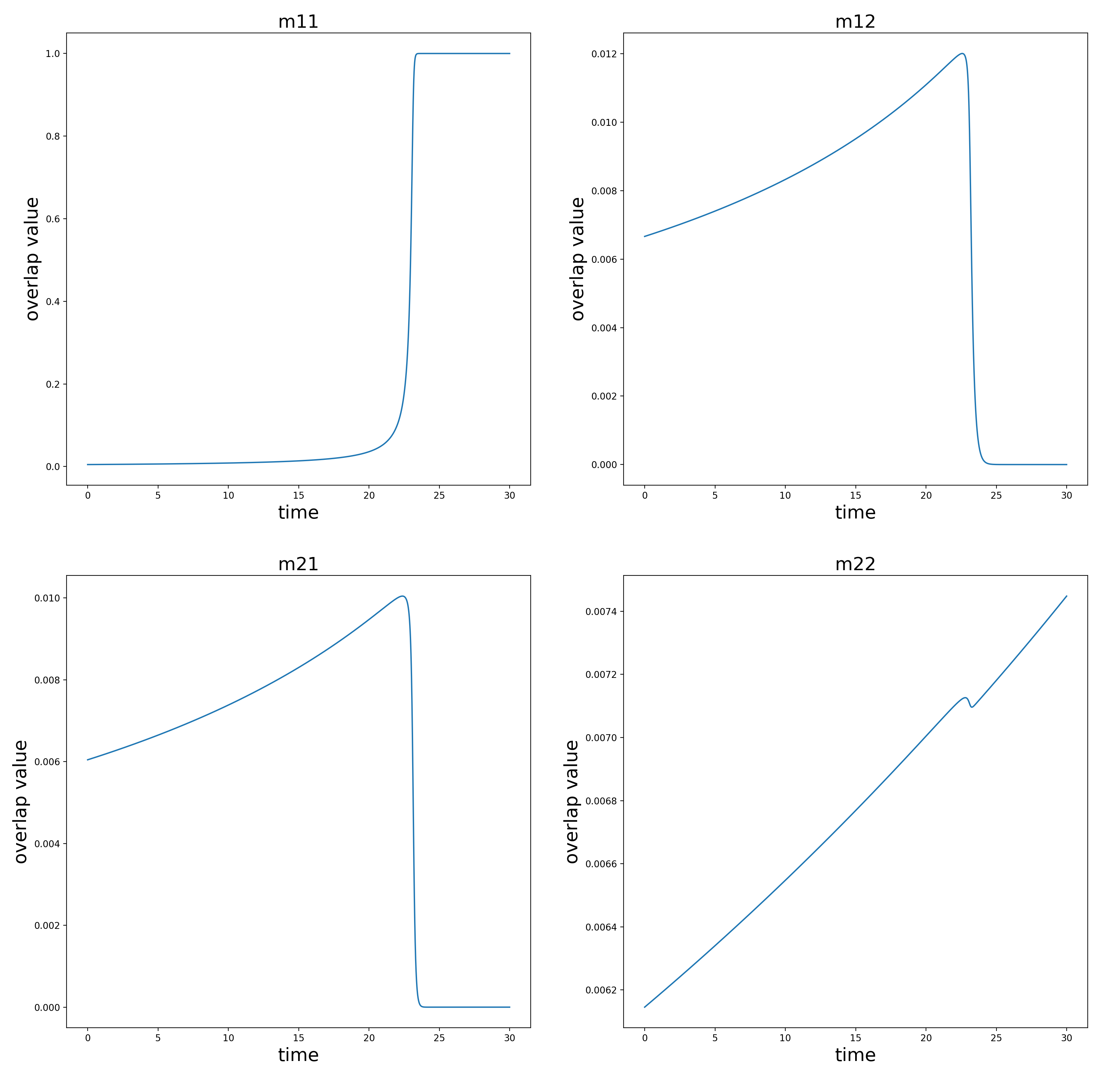
Figure 9. Evolution of the correlations $m_{ij}$ under the population dynamics in the case where $p=3$, $r=2$, $\lambda_{1}=3$ and $\lambda_{2}=1$. The SNRs are sufficiently separated to ensure exact recovery of both spikes. The figure consists of four subfigures, each zooming in on the evolution of one of the four correlations from initialization to the moment when the first correlation $m_{11}$ becomes macroscopic. In particular, $m_{12}$ and $m_{21}$ decrease rapidly once $m_{11}$ becomes macroscopic, whereas $m_{22}$ remains stable overall. The short decrease in $m_{22}$ is bounded by $\frac{\log(N)}{N}$ with high probability.

To determine the sample complexity threshold under online SGD algorithm, we control the retraction and martingale terms so that the discrete dynamics is sufficiently close to the continuous one studied in [6] over a time scale of order $\frac{\sqrt{N}}{\delta}N^{\frac{p-2}{2}}$. We show that this requires a step-size parameter of order $\log(N)^{-1}N^{-\frac{p-3}{2}}$, leading to a sample complexity of order $\log(N)N^{p-2}$. This threshold is required for efficient recovery of both spikes.

Recovery for $p=2$. In this case, the solution of (2.2) is given by

$$m_{ij}\approx m_{ij}(0)\exp\left(2\delta\lambda_{i}\lambda_{j}N^{-\frac{1}{2}}t\right)=\frac{\gamma_{ij}}{\sqrt{N}}\exp\left(2\delta\lambda_{i}\lambda_{j}N^{-\frac{1}{2}}t\right),$$ (2.4)

so that the typical time for $m_{ij}$ to reach a macroscopic threshold $\varepsilon>0$ is given by

$$T_{\varepsilon}^{(ij)}\approx\frac{\log\left(\frac{\varepsilon\sqrt{N}}{\gamma_{ij}}\right)}{2\delta\lambda_{i}\lambda_{j}}\sqrt{N}.$$

In contrast to the case where $p\geq 3$, where the quantity $\lambda_{i}\lambda_{j}\gamma_{ij}^{p-2}$ determines which correlation first escapes mediocrity, the initialization $\gamma_{ij}$ has less influence here and the time differences for the correlations to reach a macroscopic threshold are determined by the separation between the SNRs. When $\lambda_{1}>\lambda_{2}$, a sequential elimination phenomenon akin to the one observed for $p\geq 3$ occurs (see Figures 3 and 4). However, there is an important difference compared to the tensor case: once $m_{11}$ reaches the macroscopic threshold $\varepsilon>0$, the correlations $m_{12},m_{21}$ and $m_{22}$ scale as $N^{-\delta_{1}/2},N^{-\delta_{1}/2}$ and $N^{-\delta_{2}/2}$, respectively, where $\delta_{1}=1-\frac{\lambda_{2}}{\lambda_{1}}$ and $\delta_{2}=1-\frac{\lambda_{2}^{2}}{\lambda_{1}^{2}}$. We then show that $m_{11}$ must reach approximately the critical value $(\frac{\lambda_{2}}{\lambda_{1}})^{1/2}$ for $m_{12},m_{21}$ to decrease. This value is achieved in an order one time once $m_{11}$ has reached $\varepsilon$, while $m_{12},m_{21}$ still require a time of order $\log(N)$ to escape their scale of $N^{-\frac{\delta_{1}}{2}}$. In addition, we show the stability of $m_{22}$ during this first phase by controlling that it remains increasing throughout the ascending phase of $m_{11}$ and until $m_{12},m_{21}$ begin to decrease. This stability comes with an order $1$ lower bound on the logarithm of the dimension (see Theorem 3.6), involving the inverse of the gap between the SNRs, so that the case where the SNRs are close becomes sensitive to finite size effects. Weak recovery of the second direction is then possible as $m_{12},m_{21}$ descend below the scale $\frac{1}{\sqrt{N}}$. This is illustrated in Figure 10.

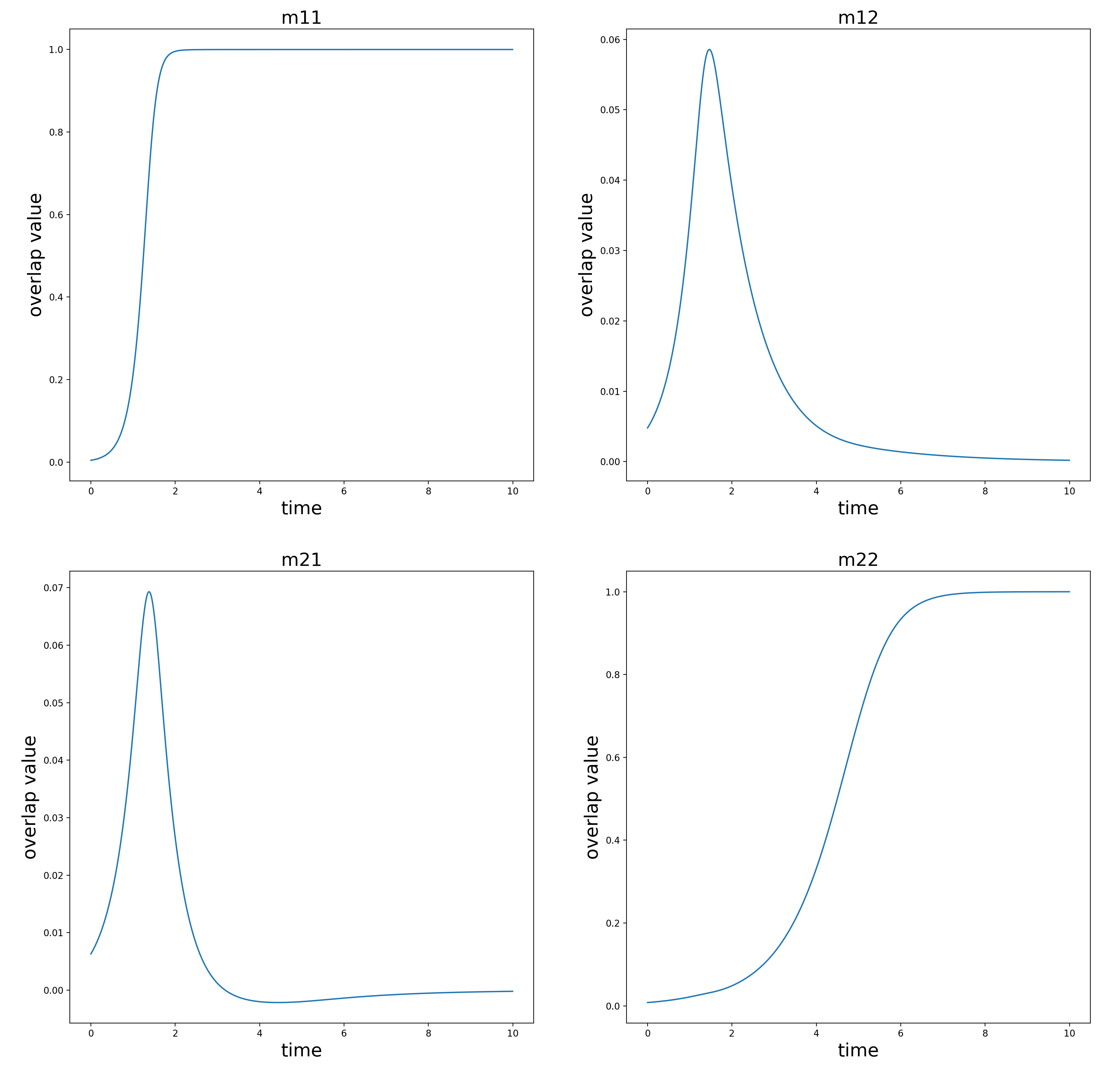
Figure 10. Evolution of the correlations $m_{ij}$ under the population dynamics in the case where $p=2,r=2,\lambda_{1}=2$ and $\lambda_{2}=1$. We observe that as $m_{11}$ reaches a certain threshold, the correlations $m_{12}$ and $m_{21}$ start to decrease, despite rising higher than in the case where $p\geq 3$.

Regarding the sample complexity, similar to the case $p\geq 3$, we control the martingale and retraction terms so that the discrete dynamics is sufficiently close to the continuous one studied in [6] over a time scale of order $\frac{\sqrt{N}}{\delta}\log(N)$. We show that this requires a step-size $\delta$ of order $\log(N)^{-1}N^{\lambda_{r}^{2}/(2\lambda_{1}^{2})}$, leading to a sample complexity for exact recovery of order $\log(N)^{2}N^{\frac{1}{2}(1-\lambda_{r}^{2}/\lambda_{1}^{2})}$. The factor $N^{\lambda_{r}^{2}/(2\lambda_{1}^{2})}$ is required to control the stability of the retraction map, which is necessary for all directions, including the first one.

2.2. Subspace recovery

As discussed in Subsection 1.2, when $\lambda_{1}=\lambda_{2}\equiv\lambda$, the spiked covariance model becomes isotropic and we shift our focus to the evolution of the eigenvalues of the matrix $\boldsymbol{M}\boldsymbol{M}^{\top}$, which we denote by $\boldsymbol{G}$. To analyze the evolution of the eigenvalues, we use eigenvalue perturbation bounds and matrix generalizations of concentration inequalities. In particular, we show that the noisy dynamics is sufficiently close to the population dynamics, which in this case takes the form of a constant coefficient algebraic Ricatti equation, i.e.,

$$\dot{\boldsymbol{G}}(t)\approx\lambda^{2}\boldsymbol{G}(t)(\boldsymbol{I}_{t}-\boldsymbol{G}(t)),$$

whose eigenvalues $\theta_{1},\ldots,\theta_{r}$ evolve according to

$$\dot{\theta_{i}}(t)\approx\lambda^{2}\theta_{i}(t)\left(1-\theta_{i}(t)\right).$$

This equation then prescribes a time horizon of order $\log(N)$ for the various bounds needed to control the noise process, leading to the sample complexities as stated in Theorem 1.11. An important difference with the full recovery case is that, at initialization, the eigenvalues of $\boldsymbol{G}$ are of order $\frac{1}{N}$. Simply adapting the bounds derived for the correlations $m_{ij}$ is not sufficient here. In particular, we develop time-dependent bounds for the martingale terms using a matrix generalization of martingale concentration inequalities [61].

3. Main results

This section presents the nonasymptotic versions of our main results stated in Subsection 1.2.

As previously discussed, we consider the online SGD algorithm starting from a random initialization, precisely $\boldsymbol{X}_{0}\sim\mu_{N\times r}$, where $\mu_{N\times r}$ denotes the uniform measure on the Stiefel manifold $\textnormal{St}(N,r)$. Our recovery guarantees, however, applies to a broader class of initial data that meets two natural conditions, that we introduce hereafter. The first condition ensures that the initial correlation is on the typical scale $\Theta(N^{-\frac{1}{2}})$.

Definition 3.1 (Condition 1).

For every $\gamma_{1}>\gamma_{2}>0$, we let $\mathcal{C}_{1}(\gamma_{1},\gamma_{2})$ denote the sequence of events given by

$$\mathcal{C}_{1}(\gamma_{1},\gamma_{2})=\left\{\boldsymbol{X}\in\textnormal{St}(N,r)\colon\frac{\gamma_{2}}{\sqrt{N}}\leq m_{ij}(\boldsymbol{X})<\frac{\gamma_{1}}{\sqrt{N}}\enspace\text{for every}\enspace 1\leq i,j\leq r\right\}.$$

We say that $\boldsymbol{X}\in\textnormal{St}(N,r)$ satisfies Condition 1 if for every $\gamma_{1}>\gamma_{2}>0$,

$$\mathbb{P}\left(\boldsymbol{X}\in\mathcal{C}_{1}(\gamma_{1},\gamma_{2})^{\textnormal{c}}\right)\leq C_{1}e^{-c_{1}\gamma_{1}^{2}}+C_{2}e^{c_{2}\gamma_{2}\sqrt{N}}+C_{3}\gamma_{2},$$

for absolute constants $C_{1},c_{1},C_{2},c_{2},C_{3}>0$.

In the special case $p=2$ and $\lambda_{1}=\cdots=\lambda_{r}$, we analyze the evolution of the eigenvalues of the matrix $\boldsymbol{G}=\boldsymbol{M}\boldsymbol{M}^{\top}$, where $\boldsymbol{M}=(m_{ij})_{1\leq i,j\leq r}$. To ensure that the eigenvalues at initialization are on the typical scale of $\Theta(N^{-1})$, we require a modified version of Condition $1$ from Definition 3.1.

Definition 3.2 (Condition 1’).

For every $\gamma_{1}>\gamma_{2}>0$, we let $\mathcal{C}_{1}^{\prime}(\gamma_{1},\gamma_{2})$ denote the sequence of events given by

$$\mathcal{C}_{1}^{\prime}(\gamma_{1},\gamma_{2})=\left\{\boldsymbol{X}\in\textnormal{St}(N,r)\colon\frac{\gamma_{2}}{N}\leq\theta_{i}(\boldsymbol{X})<\frac{\gamma_{1}}{N}\enspace\textnormal{for every}\,i\in[r]\right\}.$$

We say that $\boldsymbol{X}\in\textnormal{St}(N,r)$ satisfies Condition $1^{\prime}$ if for every $\gamma_{1}>\gamma_{2}>0$,

$$\mathbb{P}\left(\boldsymbol{X}\in\mathcal{C}_{1}^{\prime}(\gamma_{1},\gamma_{2})^{\textnormal{c}}\right)\leq C_{1}e^{-c_{1}\gamma_{1}^{2}}+C_{2}e^{-c_{2}\gamma_{2}\sqrt{N}}+C_{3}\gamma_{2},$$

for absolute constants $C_{1},c_{1},C_{2},c_{2},C_{3}>0$.

The second condition concerns the separation of the initial correlations, which is needed for the recovery when $p\geq 3$.

Definition 3.3 (Condition 2).

For every $\gamma_{1}>\gamma>0$, we let $\mathcal{C}_{2}(\gamma_{1},\gamma)$ denote the sequence of events given by

$$\mathcal{C}_{2}(\gamma_{1},\gamma)=\left\{\boldsymbol{X}\in\textnormal{St}(N,r)\colon\left|\frac{\lambda_{i}\lambda_{j}m_{ij}^{p-2}(\boldsymbol{X})}{\lambda_{k}\lambda_{\ell}m_{k\ell}^{p-2}(\boldsymbol{X})}-1\right|>\frac{\gamma}{\gamma_{1}}\enspace\text{for every}\enspace 1\leq i,j,k,\ell\leq r\right\}.$$

We say that $\boldsymbol{X}\in\textnormal{St}(N,r)$ satisfies Condition 2 if for every $\gamma_{1}>\gamma>0$,

$$\mathbb{P}\left(\boldsymbol{X}\in\mathcal{C}_{2}(\gamma_{1},\gamma)^{\textnormal{c}}\right)\leq C_{1}e^{-c_{1}\gamma_{1}^{2}}+C_{2}e^{-c_{2}\sqrt{N}\gamma}+C_{3}\left(1+\left(\frac{\lambda_{i}\lambda_{j}}{\lambda_{k}\lambda_{\ell}}\right)^{\frac{2}{p-2}}\right)^{-\frac{1}{2}}\gamma,$$

for absolute constants $C_{1},c_{1},C_{2},c_{2},C_{3}>0$.

A random matrix $\boldsymbol{X}$ uniformly distributed on $\textnormal{St}(N,r)$ satisfies the above conditions, as stated in the following lemma.

Lemma 3.4.

Every random matrix $\boldsymbol{X}\sim\mu_{N\times r}$ satisfies Condition $1$, Condition $1^{\prime}$, and Condition $2$.

The proof of Lemma 3.4 is deferred to Appendix A of the extended version of our preprint [6]. In particular, in [6] we consider the normalized Stiefel manifold $\mathcal{M}_{N,r}=\{\boldsymbol{X}\in\mathbb{R}^{N\times r}\colon\boldsymbol{X}^{\top}\boldsymbol{X}=N\boldsymbol{I}_{r}\}$ and define correlations $m_{ij}(\boldsymbol{X})$ by $m_{ij}^{(N)}(\boldsymbol{X})=\frac{\langle\boldsymbol{v}_{i},\boldsymbol{x}_{j}\rangle}{N}$, where $\boldsymbol{V}=[\boldsymbol{v}_{1},\ldots,\boldsymbol{v}_{r}]\in\mathcal{M}_{N,r}$. We then show that the invariant measure on $\mathcal{M}_{N,r}$ satisfies the three aforementioned conditions. This framework is equivalent to the one considered here, and therefore, the proofs in Appendix A of [6] can be straightforwardly generalized to $\mu_{N\times r}$.

We are now in the position to state our main results in a nonasymptotic form. Let $T$ denote the number of iterations after which we terminate the online SGD algorithm. For any set $\mathcal{E}$, let $\mathcal{T}_{\mathcal{E}}$ denote the hitting time of the set $\mathcal{E}$, i.e.,

$$\mathcal{T}_{\mathcal{E}}=\min\{t\geq 0\colon\boldsymbol{X}_{t}\in\mathcal{E}\}.$$

Additionally, we point out that the constants $K_{1},K_{2},\ldots$ and $c_{1},c_{2},\ldots$ appearing in the following statements may depend on $\sigma^{2},p,r,\{\lambda_{i}\}_{i=1}^{r}$.

Our first main result shows that for $p\geq 3$, the sample complexity threshold for efficiently recovering a permutation of all spikes $\boldsymbol{v}_{1},\ldots,\boldsymbol{v}_{r}$ must scale as $\log(N)N^{p-2}$.

Theorem 3.5 (Recovery of a permutation of all spikes for $p\geq 3$).

Let $p\geq 3$ and $\lambda_{1}\geq\cdots\geq\lambda_{r}$. Consider the sequence of online SGD outputs $(\boldsymbol{X}_{t})_{t\in\mathbb{N}}$ started from $\boldsymbol{X}_{0}$ with step-size $\delta$. Let $(i_{1}^{\ast},j_{1}^{\ast}),\ldots,(i_{r}^{\ast},j_{r}^{\ast})$ denote the greedy maximum selection of $\boldsymbol{I}_{0}$ (see (1.9) and Definition 1.4). Further, for every $\varepsilon>0$, let $R(\varepsilon)$ denote

$$R(\varepsilon)=\left\{\boldsymbol{X}\colon m_{i_{k}^{\ast}j_{k}^{\ast}}(\boldsymbol{X})\geq 1-\varepsilon\enspace\textnormal{for all}\>k\in[r]\enspace\textnormal{and}\enspace m_{ij}(\boldsymbol{X})\lesssim\log(N)^{-\frac{1}{2}}N^{-\frac{p-1}{4}}\enspace\textnormal{otherwise}\right\}.$$

Then, the following holds. For every $\gamma_{1}>\gamma_{2},\gamma>0$ and every $\varepsilon>0$, there exist $c_{0}\in(0,1)$ and $d_{0}=d_{0}(N)$ satisfying $d_{0}\to 0$ as $N\to\infty$ such that if $\boldsymbol{X}_{0}\in\mathcal{C}_{1}(\gamma_{1},\gamma_{2})\cap\mathcal{C}_{2}(\gamma_{1},\gamma)$ and $\delta>0$ verifies

$$\delta=C_{\delta}d_{0}\log(N)^{-1}N^{-\frac{p-3}{2}},$$

for a constant $C_{\delta}>0$, then

$$\mathbb{P}_{\boldsymbol{X}_{0}}\left(\mathcal{T}_{R(\varepsilon)}\lesssim T\right)\geq 1-\eta,$$

where $T$ and $\eta$ are given by

$$T=\frac{1-\left(\frac{\gamma_{2}}{\varepsilon\sqrt{N}}\right)^{p-2}}{C_{\delta}(1-c_{0})^{p-1}d_{0}\gamma_{2}^{p-2}}\log(N)N^{p-2}+\frac{1-\left(\frac{\varepsilon}{1-\varepsilon}\right)^{p-2}}{C_{\delta}(1-c_{0})^{p-1}d_{0}\varepsilon^{p-1}}\log(N)N^{\frac{p-3}{2}},$$

and

$$\begin{split}\eta&=K_{1}e^{-c_{1}\gamma_{1}^{2}}+K_{2}e^{-c_{2}(\gamma_{2}+\gamma)\sqrt{N}}+K_{3}(\gamma_{2}+\gamma)\\ &\quad+K_{4}\frac{\log(N)^{2}N^{p-2}}{d_{0}}e^{-c_{4}N}+K_{5}\log(N)e^{-c_{5}c_{0}^{2}\log(N)/d_{0}}+K_{6}\frac{d_{0}^{2}}{\log(N)}N^{-\frac{p-2}{2}}e^{-c_{6}/d_{0}^{2}},\end{split}$$

respectively.

Our second main result is for $p=2$ with sufficiently separated SNRs. We show that the sample complexity threshold for strong recovery of all spikes must diverge as $\log(N)^{2}N^{\frac{1}{2}\left(1-\frac{\lambda_{r}^{2}}{\lambda_{1}^{2}}\right)}$.

Theorem 3.6 (Exact recovery of all spikes for $p=2$).

Let $p=2$ and $\lambda_{1}\geq\cdots\geq\lambda_{r}$ such that $\lambda_{i}=\lambda_{i+1}(1+\kappa_{i})$ for every $1\leq i\leq r-1$, with $\kappa_{i}>0$ being constants of order $1$. Let $\kappa$ denote $\kappa=\min_{1\leq i\leq r-1}\kappa_{i}$. Consider the sequence of online SGD outputs $(\boldsymbol{X}_{t})_{t\in\mathbb{N}}$ started from $\boldsymbol{X}_{0}$ with step-size $\delta$. Further, for every $\varepsilon>0$ and $c_{0}\in(0,\frac{1}{2}\wedge\frac{\kappa}{2+\kappa})$, let $R(\varepsilon,c_{0})$ denote

$$R(\varepsilon,c_{0})=\left\{\boldsymbol{X}\colon m_{ii}(\boldsymbol{X})\geq 1-\varepsilon\enspace\textnormal{for all}\>i\in[r]\enspace\textnormal{and}\enspace m_{k\ell}(\boldsymbol{X})\lesssim N^{-\frac{1}{2}\left(1-\frac{1-c_{0}}{1+c_{0}}\frac{\lambda_{r}^{2}}{\lambda_{1}^{2}}\right)}\enspace\textnormal{for all}\>k\neq\ell\right\}.$$

Then, the following holds. For every $\gamma_{1}>\gamma_{2}>0$ and every $\varepsilon,\varepsilon^{\prime}>0$, there exist $c_{0}\in(0,1)$ and $d_{0}=d_{0}(N)$ satisfying $d_{0}\to 0$ as $N\to\infty$ such that if $\boldsymbol{X}_{0}\in\mathcal{C}_{1}(\gamma_{1},\gamma_{2})$ and $\delta>0$ verifies

$$\delta=\frac{C_{\delta}d_{0}N^{\frac{1}{2}\frac{1-c_{0}}{1+c_{0}}\frac{\lambda_{r}^{2}}{\lambda_{1}^{2}}}}{\log\left(\frac{2\varepsilon\sqrt{N}}{\gamma_{2}}\right)},$$

for a constant $C_{\delta}>0$, and if $\log(N)\gtrsim\frac{1}{1+\kappa}$, then

$$\mathbb{P}_{\boldsymbol{X}_{0}}\left(\mathcal{T}_{R(\varepsilon,c_{0})}\lesssim T\right)\geq 1-\eta,$$

where $T$ and $\eta$ are given by

$$T=\frac{N^{\frac{1}{2}\left(1-\frac{1-c_{0}}{1+c_{0}}\frac{\lambda_{r}^{2}}{\lambda_{1}^{2}}\right)}\log\left(\frac{2\varepsilon\sqrt{N}}{\gamma_{2}}\right)^{2}}{C_{\delta}(1-c_{0})d_{0}\gamma_{2}^{2}},$$

and

$$\begin{split}\eta&=K_{1}e^{-c_{1}\gamma_{1}^{2}}+K_{2}e^{-c_{2}\gamma_{2}\sqrt{N}}+K_{3}\gamma_{2}+K_{4}\frac{\log(N)^{2}N^{\frac{1}{2}\left(1-\frac{1-c_{0}}{1+c_{0}}\frac{\lambda_{r}^{2}}{\lambda_{1}^{2}}\right)}}{d_{0}}e^{-c_{4}N}\\ &\quad+K_{5}e^{-c_{5}c_{0}^{2}N^{\frac{1}{2}\left(\frac{1-c_{0}}{1+c_{0}}\frac{\lambda_{r}^{2}}{\lambda_{1}^{2}}\right)}/d_{0}}+K_{6}\frac{d_{0}^{2}N^{-\left(1-\frac{1-c_{0}}{1+c_{0}}\frac{\lambda_{r}^{2}}{\lambda_{1}^{2}}\right)}}{c_{0}\log(N)}e^{-c_{6}/d_{0}^{2}},\end{split}$$

respectively.

We finally state our result when the SNRs are all equal. As discussed in Subsection 1.1, we focus here on the evolution of the eigenvalues $\theta_{i}$ of the symmetric matrix $\boldsymbol{M}\boldsymbol{M}^{\top}\in\mathbb{R}^{r\times r}$, where $\boldsymbol{M}=(m_{ij})_{1\leq i,j\leq r}$ is the correlation matrix.

Theorem 3.7 (Subspace recovery for $p=2$).

Let $p=2$ and $\lambda_{1}=\cdots=\lambda_{r}\equiv\lambda$. Consider the sequence of online SGD outputs $(\boldsymbol{X}_{t})_{t\in\mathbb{N}}$ started form $\boldsymbol{X}_{0}$ with step-size $\delta$. Then, the following holds. For every $\gamma_{1}>\gamma_{2}>0$ and every $\varepsilon,\varepsilon^{\prime}>0$, there exists $d_{0}=d_{0}(N)$ satisfying $d_{0}\to 0$ as $N\to\infty$ such that if $\boldsymbol{X}_{0}\in\mathcal{C}_{1}^{\prime}(\gamma_{1},\gamma_{2})$ and $\delta>0$ verifies

$$\delta=C_{\delta}\frac{d_{0}\sqrt{N}}{\log(N)^{2}},$$

for a constant $C_{\delta}>0$, then for all $i\in[r]$,

$$\mathbb{P}_{\boldsymbol{X}_{0}}\left(\theta_{i}\left(\boldsymbol{X}_{T}\right)\geq 1-\varepsilon^{\prime}\right)\geq 1-\eta,$$

where $T$ and $\eta$ are given by

$$T=\frac{\log(N)^{2}\log(\frac{4\varepsilon N}{\gamma_{2}})}{C_{\delta}d_{0}\lambda^{2}}+\frac{\log(N)^{2}\log(\frac{1-\varepsilon^{\prime}}{\varepsilon})}{C_{\delta}d_{0}\lambda^{2}\varepsilon^{\prime}},$$

and

$$\eta=K_{1}e^{-c_{1}\gamma_{1}^{2}}+K_{2}e^{-c_{2}\gamma_{2}\sqrt{N}}+K_{3}\gamma_{2}+K_{4}\frac{\log(N)^{3}}{d_{0}}e^{-c_{4}N}+K_{5}e^{-c_{5}/d_{0}}+K_{6}\frac{\log(N)^{3}}{Nd_{0}},$$

respectively.

The proofs of the above results follow similar arguments to those in [9]. The two main steps involve controlling both the retraction term and the first-order term, which carries the phenomenology of the problem for a sufficiently small step size. Specifically, the first-order term is decomposed into a drift term and a martingale term, with the martingale term required to be negligible compared to the initialization. This requirement, along with the equivalence of the number of steps and the number of data points in online SGD, determines the step-size parameter and the sample complexity threshold. Compared to the single-spiked tensor model studied in [10], our primary challenge is that the retraction term is more complex to control. We show that it can be controlled by expanding the matrix inverse in the polar retraction as a Neumann series. Furthermore, under the chosen scaling, the signal term is larger than in [9], thus necessitating a more careful control of the higher-order signal terms in the expansion of the retraction term. In particular, some of these terms cannot be compared to the initialization scale to achieve the desired comparison inequalities. We thus compare them to the first-order signal part, up to a truncation threshold, where the upper part decays exponentially fast and can be compared to the initialization. Our second difference with respect to [10] is related to the control of the first-order noise term. In our case, under the sub-Gaussian assumption of the order-$p$ tensor, exponential forms of Doob’s inequality may be used [44, 65], resulting in faster convergence rates.

Before addressing the proof of the three main nonasymptotic results, we first provide the proofs of their asymptotic counterparts, namely Theorems 1.3, 1.5, 1.9 and 1.11.

Proof of Theorems 1.3, 1.5, 1.9 and 1.11.

According to Lemma 3.4, the uniform measure $\mu_{N\times r}$ on $\textnormal{St}(N,r)$ satisfies Condition $1$ and Condition $2$. In particular, we note that for every $\gamma_{1}>\gamma_{2}>0$, $\mu_{N\times r}\left(\mathcal{C}_{1}(\gamma_{1},\gamma_{2})\right)$ converges towards one in the large-$N$ limit, provided $\gamma_{1}$ diverges arbitrarily slowly and $\gamma_{2}$ decreases to zero arbitrarily slowly. Similarly, for every $\gamma_{1}>\gamma>0$, $\mu_{N\times r}\left(\mathcal{C}_{2}(\gamma_{1},\gamma)\right)$ converges towards one in the large-$N$ limit, provided $\gamma_{1}$ diverges arbitrarily slowly and $\gamma$ decreases to zero arbitrarily slowly. Therefore, Theorems 1.5, 1.9 and 1.11 follow straightforwardly from their nonasymptotic counterparts, namely Theorems 3.5, 3.6 and 3.7, respectively. Finally, Theorem 1.3 follows straightforwardly from Theorem 5.2 of [6], where the condition on the separation of the SNRs is expressed taking into account the value $\eta$. ∎

4. Comparison inequalities

This section presents the comparison inequalities for both the correlations and the eigenvalues of the matrix $\boldsymbol{G}=\boldsymbol{M}\boldsymbol{M}^{\top}$, which are needed to prove our main results. Before delving into these, we provide some preliminary results.

Notations. Throughout, we write $\lVert\cdot\rVert$ for the operator norm on elements of $\mathbb{R}^{r\times r}$ induced by the $L^{2}$-distance on $\mathbb{R}^{r}$. In particular, the operator norm of $\boldsymbol{A}\in\mathbb{R}^{r\times r}$ is defined as

$$\lVert\boldsymbol{A}\rVert=\max_{\boldsymbol{x}\in\mathbb{R}^{r}\backslash\{0\}}\frac{\lVert\boldsymbol{Ax}\rVert_{2}}{\lVert\boldsymbol{x}\rVert_{2}}.$$

In terms of its spectrum, the operator norm of $\boldsymbol{A}\in\mathbb{R}^{r\times r}$ corresponds to the largest singular value of $\boldsymbol{A}$, i.e., $\lVert\boldsymbol{A}\rVert=s_{\max}(\boldsymbol{A})=\sqrt{\lambda_{\max}(\boldsymbol{A}^{\top}\boldsymbol{A})}$. Moreover, we let $\lVert\boldsymbol{A}\rVert_{\textnormal{F}}$ denote the Frobenius norm of $\boldsymbol{A}$:

$$\lVert\boldsymbol{A}\rVert_{\textnormal{F}}=\left(\sum_{1\leq i,j\leq r}|\boldsymbol{A}_{ij}|^{2}\right)^{1/2}.$$

For any symmetric matrices $\boldsymbol{A}$ and $\boldsymbol{B}$, we write $\boldsymbol{A}\succeq\boldsymbol{B}$ if $\boldsymbol{A}-\boldsymbol{B}\succeq 0$, meaning that $\boldsymbol{A}-\boldsymbol{B}$ is positive semi-definite.

4.1. Preliminary results

We first recall that the loss function $\mathcal{L}_{N,r}\colon\textnormal{{St}}(N,r)\times(\mathbb{R}^{N})^{\otimes p}\to\mathbb{R}$ is given by

$$\mathcal{L}_{N,r}(\boldsymbol{X};\boldsymbol{Y})=H_{N,r}(\boldsymbol{X})+\Phi_{N,r}(\boldsymbol{X}),$$

where $H_{N,r}$ and $\Phi_{N,r}$ denote the noise and deterministic parts, respectively, which are defined by (1.4) and (1.5). To simplify notation slightly, in the remainder of the article we will write $\mathcal{L},H,\Phi$ in place of $\mathcal{L}_{N,r},H_{N,r},\Phi_{N,r}$, respectively. We assume that $\boldsymbol{W}\in(\mathbb{R}^{N})^{\otimes p}$ is an order-$p$ tensor with i.i.d. centered sub-Gaussian entries $W_{i_{1},\ldots,i_{p}}$ satisfying

$$\mathbb{E}\left[e^{tW_{i_{1},\ldots,i_{p}}}\right]\leq e^{Kt^{2}\sigma^{2}}\enspace\textnormal{for all}\enspace t\in\mathbb{R}\quad\textnormal{and}\quad\mathbb{E}\left[|W_{i_{1},\ldots,i_{p}}|^{k}\right]\leq Ck^{k/2}\sigma^{k}\enspace\textnormal{for all}\enspace k\geq 1,$$ (4.1)

where $K,C>0$ are absolute constants. Equivalently, $(W_{i_{1},\ldots,i_{p}})_{i_{1},\ldots,i_{p}}$ are i.i.d. random variables with sub-Gaussian norm $\lVert W_{i_{1},\ldots,i_{p}}\rVert_{\psi_{2}}\equiv\sigma>0$, where for any sub-Gaussian random variable $Z$, the sub-Gaussian norm $\lVert Z\rVert_{\psi_{2}}$ is defined by $\lVert Z\rVert_{\psi_{2}}=\inf\{t>0\colon\mathbb{E}\left[Z^{2}/t^{2}\right]\leq 2\}$ (see e.g. [64, Definition 2.5.6]). Since $\boldsymbol{W}$ is a sub-Gaussian $p$-tensor, the random variable $\langle\boldsymbol{v}_{i},(\nabla_{\textnormal{St}}H(\boldsymbol{X}))_{j}\rangle$ is also sub-Gaussian, as shown in the following lemma.

Lemma 4.1.

For every $\boldsymbol{v}\in\mathbb{S}^{N-1}$ and $i\in[r]$, the random variable $\langle\boldsymbol{v},(\nabla_{\textnormal{{St}}}H(\boldsymbol{X}))_{i}\rangle$ is sub-Gaussian with zero mean and sub-Gaussian norm satisfying

$$\lVert\langle\boldsymbol{v},(\nabla_{\textnormal{{St}}}H(\boldsymbol{X}))_{i}\rangle\rVert_{\psi_{2}}\leq\alpha_{1}\sigma,$$

for a constant $\alpha_{1}=\alpha_{1}(p,\{\lambda_{i}\}_{i=1}^{r})>0$.

Proof.

Using (1.8) the $i$th column vector of $\nabla_{\textnormal{St}}H(\boldsymbol{X})$ is given by

$$(\nabla_{\textnormal{St}}H(\boldsymbol{X}))_{i}=\lambda_{i}\nabla_{\boldsymbol{x}_{i}}\langle\boldsymbol{W},\boldsymbol{x}_{i}^{\otimes p}\rangle-\frac{1}{2}\sum_{j=1}^{r}\left(\lambda_{i}\boldsymbol{x}_{j}^{\top}\nabla_{\boldsymbol{x}_{i}}\langle\boldsymbol{W},\boldsymbol{x}_{i}^{\otimes p}\rangle+\lambda_{j}(\nabla_{\boldsymbol{x}_{j}}\langle\boldsymbol{W},\boldsymbol{x}_{j}^{\otimes p}\rangle)^{\top}\boldsymbol{x}_{i}\right)\boldsymbol{x}_{j},$$

where $\nabla_{\boldsymbol{x}_{i}}\langle\boldsymbol{W},\boldsymbol{x}_{i}^{\otimes p}\rangle$ has coordinates given for every $k\in[N]$ by

$$(\nabla_{\boldsymbol{x}_{i}}\langle\boldsymbol{W},\boldsymbol{x}_{i}^{\otimes p}\rangle)_{k}=p\sum_{1\leq k_{1},\ldots,k_{p-1}\leq N}W_{k,k_{1},\ldots,k_{p-1}}(x_{i})_{k_{1}}\cdots(x_{i})_{k_{p-1}}.$$

Now, for every $\boldsymbol{v}\in\mathbb{S}^{N-1}$ the inner product $\langle\boldsymbol{v},(\nabla_{\textnormal{St}}H(\boldsymbol{X}))_{i}\rangle$ can be expanded as

$$\langle\boldsymbol{v},(\nabla_{\textnormal{St}}H(\boldsymbol{X}))_{i}\rangle=p\sum_{k=1}^{N}\sum_{1\leq k_{1},\ldots,k_{p-1}\leq N}W_{k,k_{1},\ldots,k_{p-1}}f_{i}(\boldsymbol{v},\boldsymbol{X},\{\lambda_{i}\}_{i=1}^{r}),$$

where

$$\begin{split}f_{i}(\boldsymbol{v},\boldsymbol{X},\{\lambda_{i}\}_{i=1}^{r})&=\lambda_{i}v_{k}(x_{i})_{k_{1}}\cdots(x_{i})_{k_{p-1}}\\ &\quad-\frac{1}{2}\sum_{j=1}^{r}\left(\lambda_{i}(x_{j})_{k}(x_{i})_{k_{1}}\cdots(x_{i})_{k_{p-1}}+\lambda_{j}(x_{i})_{k}(x_{j})_{k_{1}}\cdots(x_{j})_{k_{p-1}}\right)\langle\boldsymbol{v},\boldsymbol{x}_{j}\rangle.\end{split}$$

This implies that the moment generating function of $\langle\boldsymbol{v},(\nabla_{\textnormal{St}}H(\boldsymbol{X}))_{i}\rangle$ is given by

$$\begin{split}\mathbb{E}\left[e^{t\langle\boldsymbol{v},(\nabla_{\textnormal{St}}H(\boldsymbol{X}))_{i}\rangle}\right]&=\prod_{k,k_{1},\ldots,k_{p-1}}\mathbb{E}\left[e^{tpW_{k,k_{1},\ldots,k_{p-1}}f_{i}(\boldsymbol{v},\boldsymbol{X},\{\lambda_{i}\}_{i=1}^{r})}\right]\\ &\leq e^{Ct^{2}p^{2}\sigma^{2}\sum_{1\leq k,k_{1},\ldots,k_{p-1}\leq N}f_{i}(\boldsymbol{v},\boldsymbol{X},\{\lambda_{i}\}_{i=1}^{r})^{2}},\end{split}$$

where we used the independence of the random variables $W_{i_{1},\ldots,i_{p}}$ and the sub-Gaussian property (4.1). Since the bound on the moment generating function characterizes the sub-Gaussian distribution (see e.g. [64, Proposition 2.5.2]), it follows that the random variable $\langle\boldsymbol{v},(\nabla_{\textnormal{St}}H(\boldsymbol{X}))_{i}\rangle$ is sub-Gaussian with zero mean and sub-Gaussian norm bounded above by

$$\begin{split}\lVert\langle\boldsymbol{v},(\nabla_{\textnormal{St}}H(\boldsymbol{X}))_{i}\rangle\rVert_{\psi_{2}}^{2}&\leq p^{2}\sigma^{2}\sum_{1\leq k,k_{1},\ldots,k_{p-1}\leq N}f_{i}(\boldsymbol{v},\boldsymbol{X},\{\lambda_{i}\}_{i=1}^{r})^{2}\\ &=p^{2}\sigma^{2}\left(\frac{1}{4}\sum_{j=1}^{r}\lambda_{j}^{2}\langle\boldsymbol{v},\boldsymbol{x}_{j}\rangle^{2}-\frac{1}{2}\lambda_{i}^{2}\langle\boldsymbol{v},\boldsymbol{x}_{i}\rangle^{2}-\frac{3}{4}\lambda_{i}^{2}\sum_{j=1}^{r}\langle\boldsymbol{v},\boldsymbol{x}_{j}\rangle^{2}\right)\\ &\leq\frac{1}{4}p^{2}\sigma^{2}\sum_{i=1}^{r}\lambda_{j}^{2},\end{split}$$

where the equality follows by the fact that $\boldsymbol{v}\in\mathbb{S}^{N-1}$ and $\boldsymbol{X}=[\boldsymbol{x}_{1},\ldots,\boldsymbol{x}_{r}]\in\textnormal{St}(N,r)$. The result follows straightforwardly. ∎

According to Subsection 1.1, the output $\boldsymbol{X}_{t}$ of the online SGD algorithm can be expanded as

$$\boldsymbol{X}_{t}=\left(\boldsymbol{X}_{t-1}-\frac{\delta}{N}\nabla_{\textnormal{{St}}}\mathcal{L}(\boldsymbol{X}_{t-1};\boldsymbol{Y}^{t})\right)\boldsymbol{P}_{t}.$$ (4.2)

Here, $\boldsymbol{P}_{t}$ denotes the projection term given by

$$\boldsymbol{P}_{t}=\left(\boldsymbol{I}_{r}+\frac{\delta^{2}}{N^{2}}\boldsymbol{\mathcal{G}}(\boldsymbol{X}_{t-1};\boldsymbol{Y}^{t})\right)^{-1/2},$$ (4.3)

where $\boldsymbol{\mathcal{G}}(\boldsymbol{X}_{t-1};\boldsymbol{Y}^{t})\in\mathbb{R}^{r\times r}$ is the Gram matrix given by

$$\boldsymbol{\mathcal{G}}(\boldsymbol{X}_{t-1};\boldsymbol{Y}^{t})=\nabla_{\textnormal{{St}}}\mathcal{L}(\boldsymbol{X}_{t-1};\boldsymbol{Y}^{t})^{\top}\nabla_{\textnormal{{St}}}\mathcal{L}(\boldsymbol{X}_{t-1};\boldsymbol{Y}^{t}).$$ (4.4)

We have the following estimate for the Frobenius norm of $\boldsymbol{\mathcal{G}}(\boldsymbol{X};\boldsymbol{Y})$.

Lemma 4.2.

There exists a constant $\alpha_{2}=\alpha_{2}(p,\{\lambda_{i}\}_{i=1}^{r})$ such that $\sup_{\boldsymbol{X}\in\textnormal{{St}}(N,r)}\mathbb{E}\left[\lVert\boldsymbol{\mathcal{G}}(\boldsymbol{X};\boldsymbol{Y})\rVert_{\textnormal{F}}\right]\leq\alpha_{2}N$. In particular, if $\delta>0$ satisfies $\delta<\left(\frac{N}{\alpha_{2}}\right)^{1/2}$, we obtain that

$$\mathbb{P}\left(\frac{\delta^{2}}{N^{2}}\lVert\boldsymbol{\mathcal{G}}(\boldsymbol{X};\boldsymbol{Y})\rVert_{\textnormal{F}}<1\right)\geq 1-\exp(-c(p)N).$$

Proof.

We first notice that

$$\lVert\boldsymbol{G}(\boldsymbol{X};\boldsymbol{Y})\rVert_{\textnormal{F}}=\lVert\nabla_{\textnormal{St}}\mathcal{L}(\boldsymbol{X};\boldsymbol{Y})^{\top}\nabla_{\textnormal{St}}\mathcal{L}(\boldsymbol{X};\boldsymbol{Y})\rVert_{\textnormal{F}}\leq\lVert\nabla_{\textnormal{St}}\mathcal{L}(\boldsymbol{X};\boldsymbol{Y})\rVert_{\textnormal{F}}^{2}.$$

Since by definition $\nabla_{\textnormal{St}}\mathcal{L}(\boldsymbol{X};\boldsymbol{Y})=\nabla\mathcal{L}(\boldsymbol{X};\boldsymbol{Y})-\frac{1}{2}\boldsymbol{X}(\nabla\mathcal{L}(\boldsymbol{X};\boldsymbol{Y})^{\top}\boldsymbol{X}+\boldsymbol{X}^{\top}\nabla\mathcal{L}(\boldsymbol{X};\boldsymbol{Y}))$, it then follows that

$$\lVert\nabla_{\textnormal{St}}\mathcal{L}(\boldsymbol{X};\boldsymbol{Y})\rVert_{\textnormal{F}}\leq\lVert\nabla\mathcal{L}(\boldsymbol{X};\boldsymbol{Y})\rVert_{\textnormal{F}}+\lVert\boldsymbol{X}^{\top}\nabla\mathcal{L}(\boldsymbol{X};\boldsymbol{Y})\rVert_{\textnormal{F}}\leq 2\lVert\nabla\mathcal{L}(\boldsymbol{X};\boldsymbol{Y})\rVert_{\textnormal{F}},$$

where for the first inequality we used the triangle inequality and the fact that $\lVert\boldsymbol{X}\nabla\mathcal{L}(\boldsymbol{X};\boldsymbol{Y})^{\top}\boldsymbol{X}\rVert_{\textnormal{F}}=\lVert\boldsymbol{X}^{\top}\nabla\mathcal{L}(\boldsymbol{X};\boldsymbol{Y})\rVert_{\textnormal{F}}$ and similarly $\lVert\boldsymbol{X}\boldsymbol{X}^{\top}\nabla\mathcal{L}(\boldsymbol{X};\boldsymbol{Y})\rVert_{\textnormal{F}}=\lVert\boldsymbol{X}^{\top}\nabla\mathcal{L}(\boldsymbol{X};\boldsymbol{Y})\rVert_{\textnormal{F}}$, while the second inequality follows by the property $\lVert\boldsymbol{X}^{\top}\boldsymbol{A}\rVert_{\textnormal{F}}\leq\lVert\boldsymbol{A}\rVert_{\textnormal{F}}$ for $\boldsymbol{X}\in\textnormal{St}(N,r)$ and $\boldsymbol{A}\in\mathbb{R}^{N\times r}$. We can write the Frobenius norm of the Euclidean gradient of $\mathcal{L}$ as

$$\lVert\nabla\mathcal{L}(\boldsymbol{X};\boldsymbol{Y})\rVert_{\textnormal{F}}^{2}=\sum_{i=1}^{r}\lVert\nabla_{\boldsymbol{x}_{i}}\mathcal{L}(\boldsymbol{X};\boldsymbol{Y})\rVert_{2}^{2},$$

where $\nabla_{\boldsymbol{x}_{i}}\mathcal{L}(\boldsymbol{X};\boldsymbol{Y})$ denotes the $i$th column of the Euclidean gradient $\nabla\mathcal{L}(\boldsymbol{X};\boldsymbol{Y})$ given by

$$\nabla_{\boldsymbol{x}_{i}}\mathcal{L}(\boldsymbol{X};\boldsymbol{Y})=\lambda_{i}\nabla_{\boldsymbol{x}_{i}}\langle\boldsymbol{W},\boldsymbol{x}_{i}^{\otimes p}\rangle+\sum_{j=1}^{r}\sqrt{N}p\lambda_{i}\lambda_{j}\langle\boldsymbol{v}_{j},\boldsymbol{x}_{i}\rangle^{p-1}\boldsymbol{v}_{j}.$$

This implies that

$$\begin{split}\mathbb{E}\left[\lVert\boldsymbol{G}(\boldsymbol{X};\boldsymbol{Y})\rVert_{\textnormal{F}}\right]&\leq 4\sum_{i=1}^{r}\left(p\lambda_{i}\mathbb{E}\left[\lVert\boldsymbol{W}\{\boldsymbol{x}_{i}\}\rVert_{2}\right]+\lVert\sum_{j=1}^{r}\sqrt{N}p\lambda_{i}\lambda_{j}\langle\boldsymbol{v}_{j},\boldsymbol{x}_{i}\rangle^{p-1}\boldsymbol{v}_{j}\rVert_{2}\right)^{2}\\ &\leq 8\sum_{i=1}^{r}\left(p^{2}\lambda_{i}^{2}\mathbb{E}\left[\lVert\boldsymbol{W}\{\boldsymbol{x}_{i}\}\rVert_{2}^{2}\right]+N\sum_{j=1}^{r}p^{2}\lambda_{i}^{2}\lambda_{j}^{2}\right),\end{split}$$

where we used the fact that $(x+y)^{2}\leq 2(x^{2}+y^{2})$, Jensen’s inequality, and the bound $\max_{i,j}|\langle\boldsymbol{v}_{j},\boldsymbol{x}_{i}\rangle|\leq 1$. Furthermore, an explicit computation of the term $\mathbb{E}\left[\lVert\boldsymbol{W}\{\boldsymbol{x}_{i}\}\rVert_{2}^{2}\right]$ gives the bound $\mathbb{E}\left[\lVert\boldsymbol{W}\{\boldsymbol{x}_{i}\}\rVert_{2}^{2}\right]\leq 2K\sigma^{2}N$. This shows the first part of the statement. For the second part, we note that

$$\lVert\boldsymbol{G}(\boldsymbol{X};\boldsymbol{Y})\rVert_{\textnormal{F}}\leq 8\sum_{i=1}^{r}\left(p^{2}\lambda_{i}^{2}\lVert\boldsymbol{W}\{\boldsymbol{x}_{i}\}\rVert_{2}^{2}+N\sum_{j=1}^{r}p^{2}\lambda_{i}^{2}\lambda_{j}^{2}\right)\leq 8\sum_{i=1}^{r}\left(p^{2}\lambda_{i}^{2}\lVert\boldsymbol{W}\rVert^{2}+N\sum_{j=1}^{r}p^{2}\lambda_{i}^{2}\lambda_{j}^{2}\right).$$

From Lemma 4.7 of [8] we then have that for every $\gamma>0$ there exists an absolute constant $c>0$ such that

$$\mathbb{P}\left(\lVert\boldsymbol{W}\rVert\geq\gamma\sqrt{N}\right)\leq 2(8p)^{Np}e^{-c\gamma^{2}N/8}.$$

Choosing $\gamma>\sqrt{2K}\sigma$, we then obtain that there is $c(p)>0$ such that

$$\lVert\boldsymbol{G}(\boldsymbol{X};\boldsymbol{Y})\rVert_{\textnormal{F}}\leq 8p^{2}\sum_{i=1}^{r}\left(\lambda_{i}^{2}2K\sigma^{2}N+N\sum_{j=1}^{r}\lambda_{i}^{2}\lambda_{j}^{2}\right)=N\alpha_{2}(p,\{\lambda_{i}\}_{i=1}^{r}).$$

with $\mathbb{P}$-probability at least $1-e^{-c(p)N}$. This completes the proof of Lemma 4.2. ∎

4.2. Comparison inequalities for correlations

The goal of this subsection is to obtain a two-sided difference inequality for the evolution of the correlations $m_{ij}(t)=m_{ij}(\boldsymbol{X}_{t})$. This will indeed be needed to prove both Theorems 3.5 and 3.6.

Proposition 4.3.

Let $\alpha_{1}=\alpha_{1}(p,\{\lambda_{i}\}_{i=1}^{r})$ and $\alpha_{2}=\alpha_{2}(p,\{\lambda_{i}\}_{i=1}^{r})$ denote the constants given by Lemmas 4.1 and 4.2, respectively. For constants $c_{0}\in(0,1)$ and $K_{N}>0$, and for every $i,j\in[r]$, we define the comparison functions $\ell_{ij}$ and $u_{ij}$ by

$$\begin{split}\ell_{ij}(t)&=(1-c_{0})m_{ij}(0)+\frac{\delta}{N}\sum_{\ell=1}^{t}\left\{-\langle\boldsymbol{v}_{i},\left(\nabla_{\textnormal{{St}}}\Phi(\boldsymbol{X}_{\ell-1})\right)_{j}\rangle-|h_{i}(\ell-1)|\right\},\\ u_{ij}(t)&=(1+c_{0})m_{ij}(0)+\frac{\delta}{N}\sum_{\ell=1}^{t}\left\{-\langle\boldsymbol{v}_{i},\left(\nabla_{\textnormal{{St}}}\Phi(\boldsymbol{X}_{\ell-1})\right)_{j}\rangle+|h_{i}(\ell-1)|\right\},\end{split}$$

where

$$|h_{i}(\ell-1)|=\frac{\delta\alpha_{2}}{2}\sum_{k=1}^{r}\left(|m_{ik}(\ell-1)|+\frac{\delta}{N}|\langle\boldsymbol{v}_{i},(\nabla_{\textnormal{{St}}}\Phi\left(\boldsymbol{X}_{\ell-1}\right))_{k}\rangle|+\frac{K_{N}\delta}{N}\right),$$

and

$$\langle\boldsymbol{v}_{i},(\nabla_{\textnormal{{St}}}\Phi(\boldsymbol{X}))_{j}\rangle=-\sqrt{N}p\lambda_{i}\lambda_{j}m_{ij}^{p-1}+\sqrt{N}\frac{p}{2}\sum_{1\leq k,\ell\leq r}\lambda_{k}m_{i\ell}m_{kj}m_{k\ell}\left(\lambda_{j}m_{kj}^{p-2}+\lambda_{\ell}m_{k\ell}^{p-2}\right).$$

Consider the sequence of outputs $(\boldsymbol{X}_{t})_{t\in\mathbb{N}}$ given by (1.6) with step-size $\delta>0$ satisfying $\delta<(N/\alpha_{2})^{1/2}$. Let $T>0$ denote a fixed time horizon. Then, for every $\gamma_{1}>\gamma_{2}>0$ there exist $c_{0}\in(0,1)$ and $K_{N}>0$ such that for every $i,j\in[r]$ and every $t\leq T$,

$$\inf_{\boldsymbol{X}_{0}\in\mathcal{C}_{1}(\gamma_{1},\gamma_{2})}\mathbb{P}_{\boldsymbol{X}_{0}}\left(\ell_{ij}(t)\leq m_{ij}(t)\leq u_{ij}(t)\right)\geq 1-\eta(\delta,c_{0},T,K_{N}),$$

where $\eta=\eta(\delta,c_{0},T,K_{N})$ is given by

$$\eta=T\exp(-c_{1}N)-2\exp\left(-c_{2}\frac{c_{0}^{2}\gamma_{2}^{2}N}{8\delta^{2}\alpha_{1}^{2}\sigma^{2}T}\right)-C\frac{2\delta^{3}r\sigma\alpha_{1}\alpha_{2}}{N^{3/2}c_{0}\gamma_{2}}T\exp\left(-c_{3}\frac{K_{N}^{2}}{2\alpha_{1}^{2}\sigma^{2}}\right).$$ (4.5)

The proof of Proposition 4.3 will be the main focus of this subsection. Our strategy involves first expanding the polar retraction term $R_{\boldsymbol{X}_{t-1}}$ from the algorithm (see (1.7)) as a Neumann series and then decompose the evolution of $m_{ij}(t)$ in three parts: the drift induced by the population loss, a martingale induced by the gradient of the noise Hamiltonian $H$, and high-order terms in $\delta$. By controlling the latter two parts, the proposition will follow.

Lemma 4.4.

Let $\alpha_{2}=\alpha_{2}(p,\{\lambda_{i}\}_{i=1}^{r})$ be the constant of Lemma 4.2. Assume that $\delta<(N/\alpha_{2})^{1/2}$. For every $T>0$, we let $\mathcal{E}_{\boldsymbol{\mathcal{G}}}=\mathcal{E}_{\boldsymbol{\mathcal{G}}}(T)$ denote the event

$$\mathcal{E}_{\boldsymbol{\mathcal{G}}}(T)=\bigcap_{1\leq t\leq T}\left\{\lVert\frac{\delta^{2}}{N^{2}}\boldsymbol{\mathcal{G}}(\boldsymbol{X}_{t-1},\boldsymbol{Y}^{t})\rVert_{\textnormal{F}}<1\right\}.$$ (4.6)

Then, there exists a constant $c(p)$ such that $\mathbb{P}\left(\mathcal{E}_{\boldsymbol{\mathcal{G}}}\right)\geq 1-T\exp(-c(p)N)$. Moreover, on the event $\mathcal{E}_{\boldsymbol{\mathcal{G}}}$, for every $i,j\in[r]$ and every $t\leq T$, it holds that

$$\left|m_{ij}(t)-\left(m_{ij}(0)-\frac{\delta}{N}\sum_{\ell=1}^{t}\langle\boldsymbol{v}_{i},(\nabla_{\textnormal{{St}}}\Phi(\boldsymbol{X}_{\ell-1}))_{j}\rangle-\frac{\delta}{N}\sum_{\ell=1}^{t}\langle\boldsymbol{v}_{i},(\nabla_{\textnormal{{St}}}H^{\ell}(\boldsymbol{X}_{\ell-1}))_{j}\rangle\right)\right|\leq\frac{\delta}{N}\sum_{\ell=1}^{t}|a_{i}(\ell-1)|,$$ (4.7)

where

$$\begin{split}|a_{i}(\ell-1)|&\leq\frac{\delta\alpha_{2}}{2}\sum_{k=1}^{r}\left(|m_{ik}(\ell-1)|+\frac{\delta}{N}|\langle\boldsymbol{v}_{i},(\nabla_{\textnormal{{St}}}\Phi\left(\boldsymbol{X}_{\ell-1}\right))_{k}\rangle|+\frac{\delta}{N}|\langle\boldsymbol{v}_{i},(\nabla_{\textnormal{{St}}}H^{\ell}\left(\boldsymbol{X}_{\ell-1})_{k}\right)\rangle|\right).\end{split}$$ (4.8)

Proof.

We begin by expanding the projection term $\boldsymbol{P}_{t}$ in (4.2) as a Neumann series. To do so, we require that $\lVert\frac{\delta^{2}}{N^{2}}\boldsymbol{\mathcal{G}}(\boldsymbol{X}_{t-1},\boldsymbol{Y}^{t})\rVert_{\textnormal{F}}<1$ for every $t\leq T$. According to Lemma 4.2, this condition holds if $\delta$ satisfies $\delta<\left(\frac{N}{\alpha_{2}}\right)^{1/2}$, leading to

$$\mathbb{P}\left(\mathcal{E}_{\boldsymbol{\mathcal{G}}}^{\textnormal{c}}\right)\leq T\,\mathbb{P}\left(\lVert\frac{\delta^{2}}{N^{2}}\boldsymbol{\mathcal{G}}(\boldsymbol{X}_{t-1},\boldsymbol{Y}^{t})\rVert_{\textnormal{F}}\geq 1\right)\leq Te^{-c(p)N}.$$

We therefore place ourselves on the event $\mathcal{E}_{\boldsymbol{\mathcal{G}}}$ for the rest of the proof. Expanding $\boldsymbol{P}_{t}$ as a Neumann series yields

$$\boldsymbol{P}_{t}=\sum_{k=0}^{\infty}(-1)^{k}{\frac{1}{2}\choose k}\frac{\delta^{2k}}{N^{2k}}\boldsymbol{\mathcal{G}}(\boldsymbol{X}_{t-1};\boldsymbol{Y}^{t})^{k}=\boldsymbol{I}_{r}+\sum_{k=1}^{\infty}(-1)^{k}{\frac{1}{2}\choose k}\frac{\delta^{2k}}{N^{2k}}\boldsymbol{\mathcal{G}}(\boldsymbol{X}_{t-1};\boldsymbol{Y}^{t})^{k}.$$

Plugging this expansion into (4.2), the online SGD output $\boldsymbol{X}_{t}$ at time $t$ can rewritten as

$$\begin{split}\boldsymbol{X}_{t}&=\boldsymbol{X}_{t-1}-\frac{\delta}{N}\nabla_{\textnormal{{St}}}\mathcal{L}(\boldsymbol{X}_{t-1};\boldsymbol{Y}^{t})\\ &\quad+\sum_{k=1}^{\infty}(-1)^{k}{\frac{1}{2}\choose k}\frac{\delta^{2k}}{N^{2k}}\left(\boldsymbol{X}_{t-1}-\frac{\delta}{N}\nabla_{\textnormal{{St}}}\mathcal{L}(\boldsymbol{X}_{t-1};\boldsymbol{Y}^{t})\right)\boldsymbol{\mathcal{G}}(\boldsymbol{X}_{t-1};\boldsymbol{Y}^{t})^{k}.\end{split}$$

For every $i,j\in[r]$ and every $1\leq t\leq T$, the evolution of the correlation $m_{ij}(\boldsymbol{X}_{t})=m_{ij}(t)$ under (1.6) is therefore given by

$$\begin{split}m_{ij}(t)&=\langle\boldsymbol{v}_{i},(\boldsymbol{X}_{t})_{j}\rangle\\ &=m_{ij}(t-1)-\frac{\delta}{N}\langle\boldsymbol{v}_{i},\left(\nabla_{\textnormal{{St}}}\mathcal{L}(\boldsymbol{X}_{t-1};\boldsymbol{Y}^{t})\right)_{j}\rangle\\ &\quad+\sum_{k=1}^{\infty}(-1)^{k}{\frac{1}{2}\choose k}\frac{\delta^{2k}}{N^{2k}}\operatorname{Tr}\left([\boldsymbol{v}_{i}]_{j}^{\top}\left(\boldsymbol{X}_{t-1}-\frac{\delta}{N}\nabla_{\textnormal{{St}}}\mathcal{L}(\boldsymbol{X}_{t-1};\boldsymbol{Y}^{t})\right)\boldsymbol{\mathcal{G}}(\boldsymbol{X}_{t-1};\boldsymbol{Y}^{t})^{k}\right),\end{split}$$

where $(\boldsymbol{X}_{t})_{j}$ denotes the $j$th column of $\boldsymbol{X}_{t}$, $\left(\nabla_{\textnormal{{St}}}\mathcal{L}(\boldsymbol{X}_{t-1};\boldsymbol{Y}_{t})\right)_{j}$ the $j$th column of $\nabla_{\textnormal{{St}}}\mathcal{L}(\boldsymbol{X}_{t-1};\boldsymbol{Y}_{t})$, and $[\boldsymbol{v}_{i}]_{j}=[\boldsymbol{0},\ldots,\boldsymbol{v}_{i},\ldots,\boldsymbol{0}]\in\mathbb{R}^{N\times r}$ the matrix in which all columns are the zero vector except column $j$ which is given by $\boldsymbol{v}_{i}$. Iterating the above expression, we then obtain that

$$\begin{split}m_{ij}(t)&=m_{ij}(0)-\frac{\delta}{N}\sum_{\ell=1}^{t}\langle\boldsymbol{v}_{i},\left(\nabla_{\textnormal{{St}}}\mathcal{L}(\boldsymbol{X}_{\ell-1};\boldsymbol{Y}^{\ell})\right)_{j}\rangle\\ &\quad+\sum_{\ell=1}^{t}\sum_{k=1}^{\infty}(-1)^{k}{\frac{1}{2}\choose k}\frac{\delta^{2k}}{N^{2k}}\operatorname{Tr}\left([\boldsymbol{v}_{i}]_{j}^{\top}\left(\boldsymbol{X}_{\ell-1}-\frac{\delta}{N}\nabla_{\textnormal{{St}}}\mathcal{L}(\boldsymbol{X}_{\ell-1};\boldsymbol{Y}^{\ell})\right)\boldsymbol{\mathcal{G}}(\boldsymbol{X}_{\ell-1};\boldsymbol{Y}^{\ell})^{k}\right).\end{split}$$

In the following, for every $i,j\in[r]$ and every $1\leq\ell\leq t$ we let $a_{ij}(\ell-1)$ denote

$$a_{ij}(\ell-1)=\sum_{k=1}^{\infty}(-1)^{k}{\frac{1}{2}\choose k}\frac{\delta^{2k}}{N^{2k}}\operatorname{Tr}\left([\boldsymbol{v}_{i}]_{j}^{\top}\left(\boldsymbol{X}_{\ell-1}-\frac{\delta}{N}\nabla_{\textnormal{{St}}}\mathcal{L}(\boldsymbol{X}_{\ell-1};\boldsymbol{Y}^{\ell})\right)\boldsymbol{\mathcal{G}}(\boldsymbol{X}_{\ell-1};\boldsymbol{Y}^{\ell})^{k}\right).$$

By Cauchy-Schwarz we then have that

$$\begin{split}|a_{ij}(\ell-1)|&\leq\sum_{k=1}^{\infty}\binom{\frac{1}{2}}{k}\frac{\delta^{2k}}{N^{2k}}\left|\operatorname{Tr}\left([\boldsymbol{v}_{i}]_{j}^{\top}\left(\boldsymbol{X}_{\ell-1}-\frac{\delta}{N}\nabla_{\textnormal{{St}}}\mathcal{L}(\boldsymbol{X}_{\ell-1};\boldsymbol{Y}^{\ell})\right)\boldsymbol{\mathcal{G}}(\boldsymbol{X}_{\ell-1};\boldsymbol{Y}^{\ell})^{k}\right)\right|\\ &\leq\sum_{k=1}^{\infty}\binom{\frac{1}{2}}{k}\lVert\frac{\delta^{2k}}{N^{2k}}\boldsymbol{\mathcal{G}}(\boldsymbol{X}_{\ell-1};\boldsymbol{Y}^{\ell})^{k}\rVert_{\textnormal{F}}\lVert[\boldsymbol{v}_{i}]_{j}^{\top}\left(\boldsymbol{X}_{\ell-1}-\frac{\delta}{N}\nabla_{\textnormal{{St}}}\mathcal{L}(\boldsymbol{X}_{\ell-1};\boldsymbol{Y}^{\ell})\right)\rVert_{\textnormal{F}}\\ &\leq\sum_{k=1}^{\infty}\binom{\frac{1}{2}}{k}C_{\boldsymbol{\mathcal{G}}}^{k-1}\lVert\frac{\delta^{2}}{N^{2}}\boldsymbol{\mathcal{G}}(\boldsymbol{X}_{\ell-1};\boldsymbol{Y}^{\ell})\rVert_{\textnormal{F}}\lVert[\boldsymbol{v}_{i}]_{j}^{\top}\left(\boldsymbol{X}_{\ell-1}-\frac{\delta}{N}\nabla_{\textnormal{{St}}}\mathcal{L}(\boldsymbol{X}_{\ell-1};\boldsymbol{Y}^{\ell})\right)\rVert_{\textnormal{F}},\end{split}$$ (4.9)

where $C_{\boldsymbol{\mathcal{G}}}=\max\lVert\frac{\delta^{2}}{N^{2}}\boldsymbol{\mathcal{G}}(\boldsymbol{X};\boldsymbol{Y})\rVert\in(0,1)$ under the event $\mathcal{E}_{\boldsymbol{\mathcal{G}}}$ for $\delta<(N/\alpha_{2})^{1/2}$. From the Newton Binomial Theorem we find that

$$\sum_{k=1}^{\infty}\binom{\frac{1}{2}}{k}C_{\boldsymbol{\mathcal{G}}}^{k-1}=\frac{1}{C_{\boldsymbol{\mathcal{G}}}}\left(\sqrt{1+C_{\boldsymbol{\mathcal{G}}}}-1\right)\leq\frac{1}{C_{\boldsymbol{\mathcal{G}}}}\frac{C_{\boldsymbol{\mathcal{G}}}}{2}=\frac{1}{2}.$$ (4.10)

Moreover, a simple computation shows that

$$\begin{split}\lVert[\boldsymbol{v}_{i}]_{j}^{\top}\left(\boldsymbol{X}_{\ell-1}-\frac{\delta}{N}\nabla_{\textnormal{{St}}}\mathcal{L}(\boldsymbol{X}_{\ell-1};\boldsymbol{Y}^{\ell})\right)\rVert_{\textnormal{F}}&=\sqrt{\sum_{k=1}^{r}\left(m_{ik}(\ell-1)-\frac{\delta}{N}\langle\boldsymbol{v}_{i},(\nabla_{\textnormal{{St}}}\mathcal{L}(\boldsymbol{X}_{\ell-1};\boldsymbol{Y}^{\ell}))_{k}\rangle\right)^{2}}\\ &\leq\sum_{k=1}^{r}\left(m_{ik}(\ell-1)-\frac{\delta}{N}\langle\boldsymbol{v}_{i},(\nabla_{\textnormal{{St}}}\mathcal{L}(\boldsymbol{X}_{\ell-1};\boldsymbol{Y}^{\ell}))_{k}\rangle\right).\end{split}$$ (4.11)

Combining (4.9)-(4.11) yields

$$|a_{ij}(\ell-1)|\leq\frac{\delta^{2}}{2N^{2}}\lVert\boldsymbol{\mathcal{G}}(\boldsymbol{X}_{\ell-1};\boldsymbol{Y}^{\ell})\rVert_{\textnormal{F}}\sum_{k=1}^{r}\left(m_{ik}(\ell-1)-\frac{\delta}{N}\langle\boldsymbol{v}_{i},(\nabla_{\textnormal{{St}}}\mathcal{L}(\boldsymbol{X}_{\ell-1};\boldsymbol{Y}^{\ell}))_{k}\rangle\right),$$

which gives the desired bound since $\lVert\boldsymbol{\mathcal{G}}(\boldsymbol{X}_{\ell-1};\boldsymbol{Y}^{\ell})\rVert_{\textnormal{F}}\leq\alpha_{2}N$ on the event $\mathcal{E}_{\boldsymbol{\mathcal{G}}}$. ∎

According to (4.7) from Lemma 4.4, we now provide an estimate for the first-order (in $\delta$) noise Hamiltonian $H$, i.e., $\frac{\delta}{N}\sum_{\ell=1}^{t}\langle\boldsymbol{v}_{i},\left(\nabla_{\textnormal{{St}}}H^{\ell}(\boldsymbol{X}_{\ell-1})\right)_{j}\rangle$.

Lemma 4.5.

Let $\alpha_{1}=\alpha_{1}(p,\{\lambda_{i}\}_{i=1}^{r})$ be the constant from Lemma 4.1. Then, for every $a>0$, there is an absolute constant $c>0$ such that

$$\sup_{\boldsymbol{X}_{0}\in\,\textnormal{{St}}(N,r)}\mathbb{P}_{\boldsymbol{X}_{0}}\left(\max_{t\leq T}\frac{\delta}{N}\left|\sum_{\ell=1}^{t}\langle\boldsymbol{v}_{i},\left(\nabla_{\textnormal{{St}}}H^{\ell}(\boldsymbol{X}_{\ell-1})\right)_{j}\rangle\right|\geq a\right)\leq 2\exp\left(-c\frac{a^{2}N^{2}}{2\delta^{2}\alpha_{1}^{2}\sigma^{2}T}\right).$$

Proof.

We let $\mathcal{F}_{t}$ denote the natural filtration associated to $\boldsymbol{X}_{1},\ldots,\boldsymbol{X}_{t}$, namely $\mathcal{F}_{t}=\sigma(\boldsymbol{X}_{\ell},\ell\leq t)$. We let $M_{t}$ denote the process

$$M_{t}=\sum_{\ell=1}^{t}\langle\boldsymbol{v}_{i},\left(\nabla_{\textnormal{{St}}}H^{\ell}(\boldsymbol{X}_{\ell-1})\right)_{j}\rangle.$$

Since

$$\mathbb{E}\left[M_{t}-M_{t-1}|\mathcal{F}_{t-1}\right]=\mathbb{E}\left[\langle\boldsymbol{v}_{i},\left(\nabla_{\textnormal{{St}}}H^{t}(\boldsymbol{X}_{t-1})\right)_{j}|\mathcal{F}_{t-1}\right]=0,$$

we have that the process $M_{t}$ is adapted to the filtration $(\mathcal{F}_{t})_{t\geq 0}$. Moreover, since $M_{s}=\mathbb{E}\left[M_{t}|\mathcal{F}_{s}\right]$, we have that $(M_{t})_{t\geq 0}$ is a martingale with respect to $(\mathcal{F}_{t})_{t\geq 0}$. Since by Lemma 4.1 the distribution of the increments $M_{t}-M_{t-1}=\langle\boldsymbol{v}_{i},(\nabla_{\textnormal{{St}}}H^{t}(\boldsymbol{X}_{t-1}))_{j}\rangle$ given $\mathcal{F}_{t-1}$ is sub-Gaussian with sub-Gaussian norm bounded by $\alpha_{1}\sigma$, we have for every $b>0$, there exists an absolute constants $C>0$ such that

$$\mathbb{E}\left[e^{b(M_{t}-M_{t-1})}|\mathcal{F}_{t-1}\right]\leq\exp\left(Cb^{2}\alpha_{1}^{2}\sigma^{2}\right).$$

The corresponding Chernoff bound applied to $M_{t}=\sum_{\ell=1}^{t}(M_{\ell}-M_{\ell-1})$ (see e.g. Theorem 2.19 of [65]) gives the tail bound: for every $t\leq T$ and every $a>0$,

$$\sup_{\boldsymbol{X}_{0}\in\textnormal{{St}}(N,r)}\mathbb{P}_{\boldsymbol{X}_{0}}\left(\frac{\delta}{N}\left|M_{t}\right|\geq a\right)\leq 2\exp\left(-c\frac{a^{2}N^{2}}{2\delta^{2}t\alpha_{1}^{2}\sigma^{2}}\right).$$

To improve this bound to the maximum $\max_{t}|M_{t}|$, we follow the remark at the end of section 3.5 from [44], noting that the random process $e^{M_{t}}$ is a submartingale. The other side of the tail bound is obtained by noting that $-M_{t}$ is also a martingale. ∎

It remains to estimate the third-order noise term in (4.8) from Lemma 4.4. To this end, we introduce a truncation level $K_{N}>0$ to be chosen later and write

$$\left|\langle\boldsymbol{v}_{i},\left(\nabla_{\textnormal{{St}}}H^{\ell}(\boldsymbol{X}_{\ell-1})\right)_{k}\rangle\right|\leq K_{N}+\left|\langle\boldsymbol{v}_{i},\left(\nabla_{\textnormal{{St}}}H^{\ell}(\boldsymbol{X}_{\ell-1})\right)_{k}\rangle\right|\mathbf{1}_{\left\{|\langle\boldsymbol{v}_{i},\left(\nabla_{\textnormal{{St}}}H^{\ell}(\boldsymbol{X}_{\ell-1})\right)_{k}\rangle|>K_{N}\right\}}.$$

Lemma 4.6.

Let $\alpha_{1}$ and $\alpha_{2}$ be the constants from Lemmas 4.1 and 4.2, respectively. Then, for every $a>0$, there are absolute constants $C,c>0$ such that

$$\begin{split}&\sup_{\boldsymbol{X}_{0}\in\textnormal{{St}}(N,r)}\mathbb{P}_{\boldsymbol{X}_{0}}\left(\max_{t\leq T}\frac{\delta^{3}\alpha_{2}}{2N^{2}}\sum_{\ell=1}^{t}\sum_{k=1}^{r}|\langle\boldsymbol{v}_{i},(\nabla_{\textnormal{{St}}}H^{\ell}\left(\boldsymbol{X}_{\ell-1}\right))_{k}\rangle|\mathbf{1}_{\{|\langle\boldsymbol{v}_{i},(\nabla_{\textnormal{{St}}}H^{\ell}\left(\boldsymbol{X}_{\ell-1}\right))_{k}\rangle|>K_{N}\}}\geq a\right)\\ &\quad\leq C\frac{\delta^{3}r\sigma\alpha_{1}\alpha_{2}}{N^{2}a}T\exp\left(-c\frac{K_{N}^{2}}{2\alpha_{1}^{2}\sigma^{2}}\right).\end{split}$$

Proof.

Since the summand is positive, the maximum over $t\leq T$ is attained at $t=T$, so it suffices to consider that case. Moreover, by Lemma 4.1 we have that the distribution of $\langle\boldsymbol{v}_{i},(\nabla_{\textnormal{{St}}}H(\boldsymbol{X}))_{j}\rangle$ is sub-Gaussian with sub-Gaussian norm bounded by $\alpha_{1}\sigma$. It therefore follows that

$$\sup_{\boldsymbol{X}\in\textnormal{{St}}(N,r)}\mathbb{E}\left[|\langle\boldsymbol{v}_{i},(\nabla_{\textnormal{{St}}}H\left(\boldsymbol{X})_{j}\right)\rangle|^{2}\right]\leq 2C\alpha_{1}^{2}\sigma^{2},$$

and that

$$\sup_{\boldsymbol{X}\in\textnormal{{St}}(N,r)}\mathbb{P}\left(|\langle\boldsymbol{v}_{i},(\nabla_{\textnormal{{St}}}H\left(\boldsymbol{X}\right))_{j}\rangle|>K_{N}\right)\leq 2\exp\left(-c\frac{K_{N}^{2}}{\alpha_{1}^{2}\sigma^{2}}\right),$$

where we used the equivalence of the sub-Gaussian properties (see e.g. [64, Proposition 2.5.2]) for both inequalities. Fix $\boldsymbol{X}_{0}\in\textnormal{{St}}(N,r)$. We then obtain for every $a>0$,

$$\begin{split}&\mathbb{P}_{\boldsymbol{X}_{0}}\left(\frac{\delta^{3}\alpha_{2}}{2N^{2}}\sum_{\ell=1}^{T}\sum_{k=1}^{r}|\langle\boldsymbol{v}_{i},(\nabla_{\textnormal{{St}}}H^{\ell}\left(\boldsymbol{X}_{\ell-1}\right))_{k}\rangle|\mathbf{1}_{\{|\langle\boldsymbol{v}_{i},(\nabla_{\textnormal{{St}}}H^{\ell}\left(\boldsymbol{X}_{\ell-1}\right))_{k}\rangle|>K_{N}\}}\geq a\right)\\ &\leq\frac{\delta^{3}r\alpha_{2}}{2N^{2}a}T\left(\sup_{\ell\leq T}\sup_{k\in[r]}\mathbb{E}_{\boldsymbol{X}_{0}}\left[|\langle\boldsymbol{v}_{i},(\nabla_{\textnormal{{St}}}H^{\ell}\left(\boldsymbol{X}_{\ell-1}\right))_{j}\rangle|\mathbf{1}_{\{|\langle\boldsymbol{v}_{i},(\nabla_{\textnormal{{St}}}H^{\ell}\left(\boldsymbol{X}_{\ell-1}\right))_{k}\rangle|>K_{N}\}}\right]\right)\\ &\leq\frac{\delta^{3}r\alpha_{2}}{2N^{2}a}T\,\sqrt{\sup_{\boldsymbol{X}}\mathbb{E}\left[|\langle\boldsymbol{v}_{i},\left(\nabla_{\textnormal{{St}}}H(\boldsymbol{X})_{k}\right)\rangle|^{2}\right]}\sqrt{\sup_{\boldsymbol{X}}\mathbb{E}\left[\mathbf{1}_{\{|\langle\boldsymbol{v}_{i},(\nabla_{\textnormal{{St}}}H\left(\boldsymbol{X}\right))_{k}\rangle|>K_{N}\}}\right]}\\ &\leq\frac{C\delta^{3}r\sigma\alpha_{1}\alpha_{2}}{N^{2}a}T\exp\left(-c\frac{K_{N}^{2}}{2\alpha_{1}^{2}\sigma^{2}}\right),\end{split}$$

where we used Markov for the first inequality and Cauchy-Schwarz for the second one. ∎

Proposition 4.3 now follows straightforwardly by combining the above three lemmas.

Proof of Proposition 4.3.

Assume that the step-size $\delta$ satisfies $\delta<\sqrt{\frac{N}{\alpha_{2}}}$, where $\alpha_{2}=\alpha_{2}(p,\{\lambda_{i}\}_{i=1}^{r})$ is the constant from Lemma 4.2. From Lemma 4.4, for every $i,j\in[r]$ and every $t\leq T$ we have the following comparison inequalities for the correlations $m_{ij}$:

$$\begin{split}m_{ij}(t)&\leq m_{ij}(0)-\frac{\delta}{N}\sum_{\ell=1}^{t}\langle\boldsymbol{v}_{i},\left(\nabla_{\textnormal{{St}}}\Phi(\boldsymbol{X}_{\ell-1})\right)_{j}\rangle+\frac{\delta}{N}\left|\sum_{\ell=1}^{t}\langle\boldsymbol{v}_{i},(\nabla_{\textnormal{{St}}}H^{\ell}(\boldsymbol{X}_{\ell-1}))_{j}\rangle\right|+\frac{\delta}{N}\sum_{\ell=1}^{t}|a_{i}(\ell-1)|,\\ m_{ij}(t)&\geq m_{ij}(0)-\frac{\delta}{N}\sum_{\ell=1}^{t}\langle\boldsymbol{v}_{i},\left(\nabla_{\textnormal{{St}}}\Phi(\boldsymbol{X}_{\ell-1})\right)_{j}\rangle-\frac{\delta}{N}\left|\sum_{\ell=1}^{t}\langle\boldsymbol{v}_{i},(\nabla_{\textnormal{{St}}}H^{\ell}(\boldsymbol{X}_{\ell-1})_{j})\rangle\right|-\frac{\delta}{N}\sum_{\ell=1}^{t}|a_{i}(\ell-1)|,\end{split}$$

with $\mathbb{P}_{\boldsymbol{X}_{0}}$-probability at least $1-T\exp\left(-c_{1}N\right)$, where $|a_{i}(\ell-1)|$ is given by (4.8). Next, we bound the noise terms by $\frac{c_{0}}{2}m_{ij}(0)$ for some constant $c_{0}\in(0,1)$ using Lemmas 4.5 and 4.6. We first note that under the event $\mathcal{C}_{1}(\gamma_{1},\gamma_{2})$, for every $i,j\in[r]$ there exists $\gamma_{ij}\in(\gamma_{2},\gamma_{1})$ such that $m_{ij}(0)=\gamma_{ij}N^{-\frac{1}{2}}$. It then follows from Lemma 4.5 that for all $t\leq T$,

$$\frac{\delta}{N}\left|\sum_{\ell=1}^{t}\langle\boldsymbol{v}_{i},(\nabla_{\textnormal{{St}}}H^{\ell}(\boldsymbol{X}_{\ell-1}))_{j}\rangle\right|\leq\frac{c_{0}\gamma_{ij}}{2\sqrt{N}},$$

with $\mathbb{P}$-probability at least $1-2\exp\left(-c_{2}\frac{c_{0}^{2}\gamma_{2}^{2}N}{8\delta^{2}\alpha_{1}^{2}\sigma^{2}T}\right)$. Moreover, we have from Lemma 4.6 that for all $t\leq T$,

$$\frac{\delta^{3}\alpha_{2}}{2N^{2}}\sum_{\ell=1}^{t}\sum_{k=1}^{r}\left|\langle\boldsymbol{v}_{i},(\nabla_{\textnormal{{St}}}H^{\ell}(\boldsymbol{X}_{\ell-1}))_{k}\rangle\right|\mathbf{1}_{\{\langle\boldsymbol{v}_{i},(\nabla_{\textnormal{{St}}}H^{\ell}(\boldsymbol{X}_{\ell-1}))_{k}\rangle>K_{N}\}}\leq\frac{c_{0}\gamma_{ij}}{2\sqrt{N}},$$

with $\mathbb{P}$-probability at least $1-\frac{2C_{1}\delta^{3}r\sigma\alpha_{1}\alpha_{2}}{N^{\frac{3}{2}}c_{0}\gamma_{2}}T\exp\left(-\frac{c_{3}K_{N}^{2}}{2\alpha_{1}^{2}\sigma^{2}}\right)$. The result then follows by standard properties of conditional probabilities.

It remains to compute $\langle\boldsymbol{v}_{i},\left(\nabla_{\textnormal{{St}}}\Phi(\boldsymbol{X})\right)_{j}\rangle$ for every $\boldsymbol{X}\in\textnormal{St}(N,r)$. According to (1.5), the $j$th column of the Euclidean gradient of the population loss $\Phi(\boldsymbol{X})$ is given by

$$(\nabla\Phi(\boldsymbol{X}))_{j}=-\sum_{k=1}^{r}p\sqrt{N}\lambda_{k}\lambda_{j}m_{kj}^{p-1}(\boldsymbol{X})\boldsymbol{v}_{k},$$

and the $j$th column of the Riemannian gradient is given by

$$\begin{split}(\nabla_{\textnormal{St}}\Phi(\boldsymbol{X}))_{j}&=-(\nabla\Phi(\boldsymbol{X}))_{j}+\frac{1}{2}\sum_{\ell=1}^{r}\left(\boldsymbol{X}^{\top}\nabla\Phi(\boldsymbol{X})+(\nabla\Phi(\boldsymbol{X}))^{\top}\boldsymbol{X}\right)_{\ell j}\boldsymbol{x}_{\ell}\\ &=-\sum_{k=1}^{r}p\sqrt{N}\lambda_{k}\lambda_{j}m_{kj}^{p-1}\boldsymbol{v}_{k}+\frac{1}{2}\sum_{1\leq k,\ell\leq r}p\sqrt{N}\lambda_{k}m_{kj}m_{k\ell}\left(\lambda_{j}m_{kj}^{p-2}+\lambda_{\ell}m_{k\ell}^{p-2}\right)\boldsymbol{x}_{\ell}.\end{split}$$

We therefore have for every $i,j\in[r]$,

$$\langle\boldsymbol{v}_{i},(\nabla_{\textnormal{{St}}}\Phi(\boldsymbol{X}))_{j}\rangle=-\sqrt{N}p\lambda_{i}\lambda_{j}m_{ij}^{p-1}+\sqrt{N}\frac{p}{2}\sum_{1\leq k,\ell\leq r}\lambda_{k}m_{i\ell}m_{kj}m_{k\ell}\left(\lambda_{j}m_{kj}^{p-2}+\lambda_{\ell}m_{k\ell}^{p-2}\right).$$

∎

4.3. Comparison inequalities for eigenvalues

In this subsection, we derive a two-sided difference inequality for the evolution of the eigenvalues $\theta_{1}(t),\ldots,\theta_{r}(t)$ of $\boldsymbol{G}_{t}=\boldsymbol{G}(\boldsymbol{X}_{t})$, where $\boldsymbol{X}_{t}$ denotes the online SGD output at time $t$. In the following, we let $\Pi_{\boldsymbol{X}}^{\textnormal{St}}$ denote the orthogonal projection on the tangent space $T_{\boldsymbol{X}}\textnormal{St}(N,r)$, i.e.,

$$\Pi_{\boldsymbol{X}}^{\textnormal{St}}(\boldsymbol{A})=\boldsymbol{A}-\boldsymbol{X}\textnormal{sym}(\boldsymbol{X}^{\top}\boldsymbol{A}),\quad\textnormal{with}\enspace\textnormal{sym}(\boldsymbol{A})=\frac{1}{2}\left(\boldsymbol{A}+\boldsymbol{A}^{\top}\right).$$

In particular, according to (1.8), for a function $F\colon\textnormal{St}(N,r)\to\mathbb{R}$, we can write $\nabla_{\textnormal{St}}F(\boldsymbol{X})=\Pi_{\boldsymbol{X}}^{\textnormal{St}}(\nabla F(\boldsymbol{X}))$. To avoid cumbersome phrasing, we will often omit stating explicitly that bounds on conditional expectations hold almost surely.

Lemma 4.7.

Let $p=2$ and $\alpha_{2}=\alpha_{2}(r,\{\lambda_{i}\}_{i=1}^{r})$ be the constant of Lemma 4.2. Consider the sequence of outputs $(\boldsymbol{X}_{t})_{t\in\mathbb{N}}$ given by (1.6) with step-size $\delta$ satisfying $\delta<(N/\alpha_{2})^{1/2}$. Let $T>0$ be a fixed time horizon. Then, there exist constants $K_{N},C,c>0$ such that for every $t\leq T$,

$$-\boldsymbol{A}_{t}\preceq\boldsymbol{G}_{t}-\left(\boldsymbol{G}_{0}+\frac{4\lambda^{2}\delta}{\sqrt{N}}\sum_{\ell=1}^{t}\boldsymbol{G}_{\ell-1}\left(\boldsymbol{I}_{r}-\boldsymbol{G}_{\ell-1}\right)-\boldsymbol{S}_{t}\right)\preceq\boldsymbol{A}_{t},$$

with $\mathbb{P}$-probability at least $1-T\exp\left(-c_{1}N\right)-4r^{2}T\exp\left(-c_{2}\frac{K_{N}^{2}}{\sigma^{2}}\right)$. Here, $\boldsymbol{S}_{t}\in\mathbb{R}^{r\times r}$ is defined by

$$\boldsymbol{S}_{t}=\frac{4\lambda\delta}{N}\sum_{\ell=1}^{t}\textnormal{sym}\left(\boldsymbol{V}^{\top}\Pi^{\textnormal{St}}_{\boldsymbol{X}_{\ell-1}}\left(\boldsymbol{W}^{\ell}\boldsymbol{X}_{\ell-1}\right)\boldsymbol{M}^{\top}_{\ell-1}\right),$$ (4.12)

and $\boldsymbol{A}_{t}\in\mathbb{R}^{r\times r}$ is given by

$$\begin{split}\boldsymbol{A}_{t}=\sum_{\ell=1}^{t}&\Big{\{}\frac{8\lambda^{2}\delta^{2}}{N^{2}}\left(4r^{2}K_{N}^{2}+\lambda^{2}N\lVert\boldsymbol{G}_{\ell-1}\rVert\right)+\frac{\alpha_{2}\delta^{2}}{N}\lVert\boldsymbol{G}_{\ell-1}\rVert\\ &+\frac{4\lambda\alpha_{2}\delta^{3}}{N^{2}}\left(2rK_{N}+\lambda\sqrt{N}\lVert\boldsymbol{G}_{\ell-1}\rVert^{1/2}\right)\lVert\boldsymbol{G}_{\ell-1}\rVert^{1/2}\Big{\}}\boldsymbol{I}_{r}.\end{split}$$ (4.13)

Proof.

From (4.2) and (4.3), the iteration for the matrix $\boldsymbol{G}_{t}=\boldsymbol{V}^{\top}\boldsymbol{X}_{t}\boldsymbol{X}_{t}^{\top}\boldsymbol{V}$ results in

$$\boldsymbol{G}_{t}=\boldsymbol{V}^{\top}\left(\boldsymbol{X}_{t-1}-\frac{\delta}{N}\nabla_{\textnormal{St}}\mathcal{L}(\boldsymbol{X}_{t-1};\boldsymbol{Y}^{t})\right)\boldsymbol{P}_{t}^{2}\left(\boldsymbol{X}_{t-1}-\frac{\delta}{N}\nabla_{\textnormal{St}}\mathcal{L}(\boldsymbol{X}_{t-1};\boldsymbol{Y}^{t})\right)^{\top}\boldsymbol{V},$$

where we used the fact that $\boldsymbol{P}_{t}^{\top}=\boldsymbol{P}_{t}$. We let $\boldsymbol{B}_{t}$ denote

$$\boldsymbol{B}_{t}=\left(\boldsymbol{X}_{t-1}^{\top}-\frac{\delta}{N}\left(\nabla_{\textnormal{St}}\mathcal{L}(\boldsymbol{X}_{t-1};\boldsymbol{Y}^{t})\right)^{\top}\right)\boldsymbol{V}.$$

In the following, we place ourselves on the event $\mathcal{E}_{\boldsymbol{\mathcal{G}}}(T)=\bigcap_{1\leq t\leq T}\left\{\lVert\frac{\delta^{2}}{N^{2}}\boldsymbol{\mathcal{G}}(\boldsymbol{X}_{t-1};\boldsymbol{Y}^{t})\rVert_{\textnormal{F}}<1\right\}$. According to Lemma 4.4, we have that $\mathbb{P}\left(\mathcal{E}_{\boldsymbol{\mathcal{G}}}\right)\geq 1-T\exp(-c_{1}N)$ for every $p\geq 2$. As in the proof of Lemma 4.4, we can therefore expand the projection term $\boldsymbol{P}_{t}^{2}$ as a Neumann series:

$$\boldsymbol{P}_{t}^{2}=\left(\boldsymbol{I}_{r}+\frac{\delta^{2}}{N^{2}}\boldsymbol{\mathcal{G}}(\boldsymbol{X}_{t-1};\boldsymbol{Y}^{t})\right)^{-1}=\sum_{k=0}^{\infty}(-1)^{k}\frac{\delta^{2k}}{N^{2k}}\boldsymbol{\mathcal{G}}(\boldsymbol{X}_{t-1};\boldsymbol{Y}^{t})^{k}.$$

We write the output $\boldsymbol{G}_{t}$ at time $t$ as

$$\boldsymbol{G}_{t}=\boldsymbol{B}_{t}^{\top}\boldsymbol{P}_{t}^{2}\boldsymbol{B}_{t}=\boldsymbol{B}_{t}^{\top}\boldsymbol{B}_{t}+\sum_{k=1}^{\infty}(-1)^{k}\frac{\delta^{2k}}{N^{2k}}\boldsymbol{\mathcal{G}}(\boldsymbol{X}_{t-1};\boldsymbol{Y}^{t})^{k}.$$

We now want to expand the matrix $\boldsymbol{B}_{t}$ by explicitly computing the Riemannian gradient. Since $p=2$ and $\lambda_{1}=\cdots=\lambda_{r}\equiv\lambda$, the loss function $\mathcal{L}(\boldsymbol{X};\boldsymbol{Y})$ given by (1.3) reduces to

$$\mathcal{L}(\boldsymbol{X};\boldsymbol{Y})=\lambda\sum_{i=1}^{r}\boldsymbol{x}_{i}^{\top}\boldsymbol{W}\boldsymbol{x}_{i}-\sqrt{N}\lambda^{2}\sum_{i,j=1}^{r}m_{ij}^{2}(\boldsymbol{X}).$$

The Euclidean gradient $\nabla\mathcal{L}(\boldsymbol{X};\boldsymbol{Y})$ is then given by

$$\nabla\mathcal{L}(\boldsymbol{X};\boldsymbol{Y})=2\lambda\boldsymbol{W}\boldsymbol{X}-2\sqrt{N}\lambda^{2}\boldsymbol{V}\boldsymbol{M},$$

where $\boldsymbol{M}=(m_{ij})_{1\leq i,j\leq r}=\boldsymbol{V}^{\top}\boldsymbol{X}\in\mathbb{R}^{r\times r}$, and using (1.8), the Riemannian gradient is given by

$$\nabla_{\textnormal{St}}\mathcal{L}(\boldsymbol{X};\boldsymbol{Y})=2\lambda\Pi^{\textnormal{St}}_{\boldsymbol{X}}(\boldsymbol{W}\boldsymbol{X})-2\sqrt{N}\lambda^{2}\boldsymbol{V}\boldsymbol{M}+2\sqrt{N}\lambda^{2}\boldsymbol{X}\boldsymbol{M}^{\top}\boldsymbol{M},$$ (4.14)

where we recall that $\Pi^{\textnormal{St}}_{\boldsymbol{X}}$ denotes the projection onto $T_{\boldsymbol{X}}\textnormal{St}(N,r)$. This implies that

$$\begin{split}\boldsymbol{G}_{t}&=\boldsymbol{G}_{t-1}+\frac{4\delta\lambda^{2}}{\sqrt{N}}\boldsymbol{G}_{t-1}\left(\boldsymbol{I}_{r}-\boldsymbol{G}_{t-1}\right)-\frac{4\delta\lambda}{N}\textnormal{sym}\left(\boldsymbol{V}^{\top}\Pi^{\textnormal{St}}_{\boldsymbol{X}_{t-1}}\left(\boldsymbol{W}^{t}\boldsymbol{X}_{t-1}\right)\boldsymbol{M}_{t-1}^{\top}\right)\\ &\quad+\frac{\delta^{2}}{N^{2}}\boldsymbol{V}^{\top}\nabla_{\textnormal{St}}\mathcal{L}\left(\boldsymbol{X}_{t-1};\boldsymbol{Y}^{t}\right)\left(\nabla_{\textnormal{St}}\mathcal{L}\left(\boldsymbol{X}_{t-1};\boldsymbol{Y}^{t}\right)\right)^{\top}\boldsymbol{V}\\ &\quad+\sum_{k=1}^{\infty}(-1)^{k}\frac{\delta^{2k}}{N^{2k}}\boldsymbol{B}_{t}^{\top}\boldsymbol{\mathcal{G}}(\boldsymbol{X}_{t-1};\boldsymbol{Y}^{t})^{k}\boldsymbol{B}_{t}.\end{split}$$ (4.15)

The remainder of the proof focuses on estimating the terms in (4.15) that are of order $2$ or higher in $\delta$.

First, we consider the summand

$$\frac{\delta^{2}}{N^{2}}\boldsymbol{V}^{\top}\nabla_{\textnormal{St}}\mathcal{L}(\boldsymbol{X}_{t-1};\boldsymbol{Y}^{t})\left(\nabla_{\textnormal{St}}\mathcal{L}(\boldsymbol{X}_{t-1};\boldsymbol{Y}^{t})\right)^{\top}\boldsymbol{V},$$

and observe that

$$\begin{split}\frac{\delta^{2}}{N^{2}}\boldsymbol{V}^{\top}\nabla_{\textnormal{St}}\mathcal{L}(\boldsymbol{X}_{t-1};\boldsymbol{Y}^{t})\left(\nabla_{\textnormal{St}}\mathcal{L}(\boldsymbol{X}_{t-1};\boldsymbol{Y}^{t})\right)^{\top}\boldsymbol{V}&\preceq\frac{\delta^{2}}{N^{2}}\lVert\boldsymbol{V}^{\top}\nabla_{\textnormal{St}}\mathcal{L}(\boldsymbol{X}_{t-1};\boldsymbol{Y}^{t})\rVert^{2}\boldsymbol{I}_{r},\\ \frac{\delta^{2}}{N^{2}}\boldsymbol{V}^{\top}\nabla_{\textnormal{St}}\mathcal{L}(\boldsymbol{X}_{t-1};\boldsymbol{Y}^{t})\left(\nabla_{\textnormal{St}}\mathcal{L}(\boldsymbol{X}_{t-1};\boldsymbol{Y}^{t})\right)^{\top}\boldsymbol{V}&\succeq-\frac{\delta^{2}}{N^{2}}\lVert\boldsymbol{V}^{\top}\nabla_{\textnormal{St}}\mathcal{L}(\boldsymbol{X}_{t-1};\boldsymbol{Y}^{t})\rVert^{2}\boldsymbol{I}_{r}.\end{split}$$

We therefore want to estimate the operator norm of $\boldsymbol{V}^{\top}\nabla_{\textnormal{St}}\mathcal{L}\left(\boldsymbol{X}_{t-1};\boldsymbol{Y}_{t}\right)$. From (4.14), we have that

$$\boldsymbol{V}^{\top}\nabla_{\textnormal{St}}\mathcal{L}\left(\boldsymbol{X}_{t-1};\boldsymbol{Y}_{t}\right)=2\lambda\boldsymbol{V}^{\top}\Pi^{\textnormal{St}}_{\boldsymbol{X}_{t-1}}\left(\boldsymbol{W}^{t}\boldsymbol{X}_{t-1}\right)-2\sqrt{N}\lambda^{2}\boldsymbol{M}_{t-1}\left(\boldsymbol{I}_{r}-\boldsymbol{M}_{t-1}^{\top}\boldsymbol{M}_{t-1}\right),$$

which gives the bound

$$\lVert\boldsymbol{V}^{\top}\nabla_{\textnormal{St}}\mathcal{L}\left(\boldsymbol{X}_{t-1};\boldsymbol{Y}_{t}\right)\rVert\leq 2\lambda\lVert\boldsymbol{V}^{\top}\Pi^{\textnormal{St}}_{\boldsymbol{X}_{t-1}}\left(\boldsymbol{W}^{t}\boldsymbol{X}_{t-1}\right)\rVert+2\sqrt{N}\lambda^{2}\lVert\boldsymbol{M}_{t-1}\rVert,$$ (4.16)

where we used the fact that $\lVert\boldsymbol{I}_{r}-\boldsymbol{M}_{t-1}^{\top}\boldsymbol{M}_{t-1}\rVert\leq 1$, since $\boldsymbol{M}_{t-1}^{\top}\boldsymbol{M}_{t-1}$ is positive semi-definite with its operator norm bounded above by $1$. Additionally, we can bound the operator norm of $\boldsymbol{V}^{\top}\Pi^{\textnormal{St}}_{\boldsymbol{X}_{t-1}}\left(\boldsymbol{W}^{t}\boldsymbol{X}_{t-1}\right)$ as follows:

$$\begin{split}\lVert\boldsymbol{V}^{\top}\Pi^{\textnormal{St}}_{\boldsymbol{X}_{t-1}}\left(\boldsymbol{W}^{t}\boldsymbol{X}_{t-1}\right)\rVert&=\lVert\boldsymbol{V}^{\top}\boldsymbol{W}^{t}\boldsymbol{X}_{t-1}-\boldsymbol{V}^{\top}\boldsymbol{X}_{t-1}\textnormal{sym}\left(\boldsymbol{X}_{t-1}^{\top}\boldsymbol{W}^{t}\boldsymbol{X}_{t-1}\right)\rVert\\ &\leq\lVert\boldsymbol{V}^{\top}\boldsymbol{W}^{t}\boldsymbol{X}_{t-1}\rVert+\lVert\boldsymbol{X}_{t-1}^{\top}\boldsymbol{W}^{t}\boldsymbol{X}_{t-1}\rVert,\end{split}$$ (4.17)

where we used the fact that $\lVert\boldsymbol{V}^{\top}\boldsymbol{X}_{t-1}\rVert=\lVert\boldsymbol{M}_{t-1}\rVert\leq 1$ and the fact that the matrix $\boldsymbol{W}^{t}$ is symmetric. Combining (4.16) and (4.17) yields

$$\begin{split}\lVert\boldsymbol{V}^{\top}\nabla_{\textnormal{St}}\mathcal{L}\left(\boldsymbol{X}_{t-1};\boldsymbol{Y}_{t}\right)\rVert^{2}&\leq 2\left(4\lambda^{2}\lVert\boldsymbol{V}^{\top}\Pi^{\textnormal{St}}_{\boldsymbol{X}_{t-1}}\left(\boldsymbol{W}^{t}\boldsymbol{X}_{t-1}\right)\rVert^{2}+4N\lambda^{4}\lVert\boldsymbol{M}_{t-1}\rVert^{2}\right)\\ &\leq 8\lambda^{2}\left(2\lVert\boldsymbol{V}^{\top}\boldsymbol{W}^{t}\boldsymbol{X}_{t-1}\rVert^{2}+2\lVert\boldsymbol{X}_{t-1}^{\top}\boldsymbol{W}^{t}\boldsymbol{X}_{t-1}\rVert^{2}+N\lambda^{2}\lVert\boldsymbol{G}_{t-1}\rVert\right),\end{split}$$ (4.18)

where we used the fact that $(a+b)^{2}\leq 2(a^{2}+b^{2})$.

Now, consider the higher order terms in $\delta$ from (4.15), i.e.,

$$\sum_{k=1}^{\infty}(-1)^{k}\frac{\delta^{2k}}{N^{2k}}\boldsymbol{B}_{t}^{\top}\boldsymbol{\mathcal{G}}(\boldsymbol{X}_{t-1};\boldsymbol{Y}^{t})^{k}\boldsymbol{B}_{t}.$$

Note first that for every $k\geq 1$,

$$-\lVert\boldsymbol{\mathcal{G}}\rVert^{k-1}\boldsymbol{B}_{t}^{\top}\boldsymbol{\mathcal{G}}\boldsymbol{B}_{t}\preceq\boldsymbol{B}_{t}^{\top}\boldsymbol{\mathcal{G}}^{k}\boldsymbol{B}_{t}\preceq\lVert\boldsymbol{\mathcal{G}}\rVert^{k-1}\boldsymbol{B}_{t}^{\top}\boldsymbol{\mathcal{G}}\boldsymbol{B}_{t}.$$

Indeed, since $\boldsymbol{\mathcal{G}}$ is positive semi-definite, for every $\boldsymbol{y}\in\mathbb{R}^{r}$ we can write

$$\begin{split}\boldsymbol{y}^{\top}\boldsymbol{B}_{t}^{\top}\left(\boldsymbol{\mathcal{G}}^{k}-\lVert\boldsymbol{\mathcal{G}}\rVert^{k-1}\boldsymbol{\mathcal{G}}\right)\boldsymbol{B}_{t}\boldsymbol{y}&=\boldsymbol{y}^{\top}\boldsymbol{B}_{t}^{\top}\boldsymbol{\mathcal{G}}^{1/2}\left(\boldsymbol{\mathcal{G}}^{k-1}-\lVert\boldsymbol{\mathcal{G}}\rVert^{k-1}\boldsymbol{I}_{r}\right)\boldsymbol{\mathcal{G}}^{1/2}\boldsymbol{B}_{t}\boldsymbol{y}\\ &\leq\boldsymbol{z}^{\top}\left(\boldsymbol{\mathcal{G}}^{k-1}-\lVert\boldsymbol{\mathcal{G}}^{k-1}\rVert\boldsymbol{I}_{r}\right)\boldsymbol{z}\leq 0,\end{split}$$

where $\boldsymbol{z}=\boldsymbol{\mathcal{G}}^{1/2}\boldsymbol{B}_{t}\boldsymbol{y}$. The other inequality follows similarly. This implies that

$$-\sum_{k=1}^{\infty}(-1)^{k}\frac{\delta^{2k}}{N^{2k}}\lVert\boldsymbol{\mathcal{G}}\rVert^{k-1}\boldsymbol{B}_{t}^{\top}\boldsymbol{\mathcal{G}}\boldsymbol{B}_{t}\preceq\sum_{k=1}^{\infty}(-1)^{k}\frac{\delta^{2k}}{N^{2k}}\boldsymbol{B}_{t}^{\top}\boldsymbol{\mathcal{G}}(\boldsymbol{X}_{t-1};\boldsymbol{Y}^{t})^{k}\boldsymbol{B}_{t}\preceq\sum_{k=1}^{\infty}(-1)^{k}\frac{\delta^{2k}}{N^{2k}}\lVert\boldsymbol{\mathcal{G}}\rVert^{k-1}\boldsymbol{B}_{t}^{\top}\boldsymbol{\mathcal{G}}\boldsymbol{B}_{t},$$

where

$$\sum_{k=1}^{\infty}(-1)^{k}\frac{\delta^{2k}}{N^{2k}}\lVert\boldsymbol{\mathcal{G}}\rVert^{k-1}\boldsymbol{B}_{t}^{\top}\boldsymbol{\mathcal{G}}\boldsymbol{B}_{t}=-\left(\sum_{k=0}^{\infty}(-1)^{k}\lVert\frac{\delta^{2}}{N^{2}}\boldsymbol{\mathcal{G}}\rVert^{k}\right)\frac{\delta^{2}}{N^{2}}\boldsymbol{B}_{t}^{\top}\boldsymbol{\mathcal{G}}\boldsymbol{B}_{t}=-\frac{1}{1+\alpha_{2}\frac{\delta^{2}}{N}}\frac{\delta^{2}}{N^{2}}\boldsymbol{B}_{t}^{\top}\boldsymbol{\mathcal{G}}\boldsymbol{B}_{t},$$

where we used the fact that $\max\lVert\frac{\delta^{2}}{N^{2}}\boldsymbol{\mathcal{G}}\rVert\leq\alpha_{2}\frac{\delta^{2}}{N}$ on the event $\mathcal{E}_{\boldsymbol{\mathcal{G}}}$. Therefore, we have that

$$\begin{split}\sum_{k=1}^{\infty}(-1)^{k}\frac{\delta^{2k}}{N^{2k}}\boldsymbol{B}_{t}^{\top}\boldsymbol{\mathcal{G}}(\boldsymbol{X}_{t-1};\boldsymbol{Y}^{t})^{k}\boldsymbol{B}_{t}&\preceq-\frac{1}{1+\alpha_{2}\frac{\delta^{2}}{N}}\frac{\delta^{2}}{N^{2}}\boldsymbol{B}_{t}^{\top}\boldsymbol{\mathcal{G}}\boldsymbol{B}_{t},\\ \sum_{k=1}^{\infty}(-1)^{k}\frac{\delta^{2k}}{N^{2k}}\boldsymbol{B}_{t}^{\top}\boldsymbol{\mathcal{G}}(\boldsymbol{X}_{t-1};\boldsymbol{Y}^{t})^{k}\boldsymbol{B}_{t}&\succeq\frac{1}{1+\alpha_{2}\frac{\delta^{2}}{N}}\frac{\delta^{2}}{N^{2}}\boldsymbol{B}_{t}^{\top}\boldsymbol{\mathcal{G}}\boldsymbol{B}_{t},\\ \end{split}$$ (4.19)

It remains to bound the operator norm of $\boldsymbol{B}_{t}^{\top}\boldsymbol{\mathcal{G}}\boldsymbol{B}_{t}$:

$$\begin{split}&\frac{\delta^{2}}{N^{2}}\boldsymbol{B}_{t}^{\top}\boldsymbol{\mathcal{G}}(\boldsymbol{X}_{t-1};\boldsymbol{Y}^{t})\boldsymbol{B}_{t}\\ &=\frac{\delta^{2}}{N^{2}}\boldsymbol{M}_{t-1}\boldsymbol{\mathcal{G}}(\boldsymbol{X}_{t-1};\boldsymbol{Y}^{t})\boldsymbol{M}_{t-1}^{\top}-\frac{2\delta^{3}}{N^{3}}\textnormal{sym}\left(\boldsymbol{V}^{\top}\nabla_{\textnormal{St}}\mathcal{L}\left(\boldsymbol{X}_{t-1};\boldsymbol{Y}^{t}\right)\boldsymbol{\mathcal{G}}(\boldsymbol{X}_{t-1};\boldsymbol{Y}^{t})\boldsymbol{M}_{t-1}^{\top}\right)\\ &\quad+\frac{\delta^{4}}{N^{4}}\boldsymbol{V}^{\top}\nabla_{\textnormal{St}}\mathcal{L}\left(\boldsymbol{X}_{t-1};\boldsymbol{Y}^{t}\right)\boldsymbol{\mathcal{G}}(\boldsymbol{X}_{t-1};\boldsymbol{Y}^{t})\left(\nabla_{\textnormal{St}}\mathcal{L}(\boldsymbol{X}_{t-1};\boldsymbol{Y}^{t})\right)^{\top}\boldsymbol{V}.\end{split}$$

The operator norm of the first summand is bounded above by

$$\begin{split}\frac{\delta^{2}}{N^{2}}\lVert\boldsymbol{M}_{t-1}\boldsymbol{\mathcal{G}}(\boldsymbol{X}_{t-1};\boldsymbol{Y}^{t})\boldsymbol{M}_{t-1}^{\top}\rVert&=\frac{\delta^{2}}{N^{2}}\lVert\boldsymbol{M}_{t-1}\nabla_{\textnormal{St}}\mathcal{L}(\boldsymbol{X}_{t-1};\boldsymbol{Y}^{t})\rVert^{2}\\ &\leq\frac{\delta^{2}}{N^{2}}\lVert\boldsymbol{M}_{t-1}\rVert^{2}\lVert\nabla_{\textnormal{St}}\mathcal{L}(\boldsymbol{X}_{t-1};\boldsymbol{Y}^{t})\rVert^{2}\\ &\leq\alpha_{2}\frac{\delta^{2}}{N}\lVert\boldsymbol{G}_{t-1}\rVert,\end{split}$$

where we used the fact that $\lVert\nabla_{\textnormal{St}}\mathcal{L}(\boldsymbol{X}_{t-1};\boldsymbol{Y}^{t})\rVert^{2}=\lVert\boldsymbol{\mathcal{G}}(\boldsymbol{X}_{t-1};\boldsymbol{Y}^{t})\rVert$. For the second summand, we have that

$$\begin{split}&\frac{2\delta^{3}}{N^{3}}\lVert\mbox{sym}\left(\boldsymbol{V}^{\top}\nabla_{\textnormal{St}}\mathcal{L}\left(\boldsymbol{X}_{t-1};\boldsymbol{Y}^{t}\right)\boldsymbol{\mathcal{G}}(\boldsymbol{X}_{t-1};\boldsymbol{Y}^{t})\boldsymbol{M}_{t-1}^{\top}\right)\rVert\\ &\leq\frac{2\delta^{3}}{N^{3}}\lVert\boldsymbol{\mathcal{G}}(\boldsymbol{X}_{t-1};\boldsymbol{Y}^{t})\rVert\lVert\boldsymbol{V}^{\top}\nabla_{\textnormal{St}}\mathcal{L}(\boldsymbol{X}_{t-1};\boldsymbol{Y}^{t})\rVert\lVert\boldsymbol{M}_{t-1}\rVert\\ &\leq\frac{2\alpha_{2}\delta^{3}}{N^{2}}\left(2\lambda\lVert\boldsymbol{V}^{\top}\boldsymbol{W}^{t}\boldsymbol{X}_{t-1}\rVert+2\lambda\lVert\boldsymbol{X}_{t-1}^{\top}\boldsymbol{W}^{t}\boldsymbol{X}_{t-1}\rVert+2\sqrt{N}\lambda^{2}\lVert\boldsymbol{M}_{t-1}\rVert\right)\lVert\boldsymbol{M}_{t-1}\rVert,\end{split}$$

where the last inequality follows by (4.16) and (4.17). Finally, the third term is bounded in operator norm as follows:

$$\begin{split}&\frac{\delta^{4}}{N^{4}}\lVert\boldsymbol{V}^{\top}\nabla_{\textnormal{St}}\mathcal{L}\left(\boldsymbol{X}_{t-1};\boldsymbol{Y}^{t}\right)\boldsymbol{\mathcal{G}}(\boldsymbol{X}_{t-1};\boldsymbol{Y}^{t})\left(\nabla_{\textnormal{St}}\mathcal{L}(\boldsymbol{X}_{t-1};\boldsymbol{Y}^{t})\right)^{\top}\boldsymbol{V}\rVert\\ &=\frac{\delta^{4}}{N^{4}}\lVert\boldsymbol{V}^{\top}\nabla_{\textnormal{St}}\mathcal{L}\left(\boldsymbol{X}_{t-1};\boldsymbol{Y}^{t}\right)\left(\nabla_{\textnormal{St}}\mathcal{L}(\boldsymbol{X}_{t-1};\boldsymbol{Y}^{t})\right)^{\top}\rVert^{2}\\ &\leq\frac{\delta^{4}}{N^{4}}\lVert\boldsymbol{V}^{\top}\nabla_{\textnormal{St}}\mathcal{L}(\boldsymbol{X}_{t-1};\boldsymbol{Y}^{t})\rVert^{2}\lVert\boldsymbol{\mathcal{G}}(\boldsymbol{X}_{t-1};\boldsymbol{Y}^{t})\rVert\\ &\leq 8\lambda^{2}\frac{\alpha_{2}\delta^{4}}{N^{3}}\left(2\lVert\boldsymbol{V}^{\top}\boldsymbol{W}^{t}\boldsymbol{X}_{t-1}\rVert^{2}+2\lVert\boldsymbol{X}_{t-1}^{\top}\boldsymbol{W}^{t}\boldsymbol{X}_{t-1}\rVert^{2}+N\lambda^{2}\lVert\boldsymbol{G}_{t-1}\rVert\right),\end{split}$$

where we used (4.18) for the last inequality.

Combining the last four estimates with (4.19) and from (4.15) and (4.18), we finally obtain the partial ordering

$$\begin{split}\boldsymbol{G}_{t}&\preceq\boldsymbol{G}_{t-1}+\frac{4\lambda^{2}\delta}{\sqrt{N}}\boldsymbol{G}_{t-1}\left(\boldsymbol{I}_{r}-\boldsymbol{G}_{t-1}\right)-\frac{4\lambda\delta}{N}\mbox{sym}\left(\boldsymbol{V}^{\top}\Pi^{\textnormal{St}}_{\boldsymbol{X}_{t-1}}\left(\boldsymbol{W}^{t}\boldsymbol{X}_{t-1}\right)\boldsymbol{M}_{t-1}^{\top}\right)\\ &\enspace+\frac{8\lambda^{2}\delta^{2}}{N^{2}}\left(1+\alpha_{2}\frac{\delta^{2}}{N}\frac{1}{1+\alpha_{2}\frac{\delta^{2}}{N}}\right)\left(2\lVert\boldsymbol{V}^{\top}\boldsymbol{W}^{t}\boldsymbol{X}_{t-1}\rVert^{2}+2\lVert\boldsymbol{X}_{t-1}^{\top}\boldsymbol{W}^{t}\boldsymbol{X}_{t-1}\rVert^{2}+N\lambda^{2}\lVert\boldsymbol{G}_{t-1}\rVert\right)\boldsymbol{I}_{r}\\ &\enspace+\frac{1}{1+\alpha_{2}\frac{\delta^{2}}{N}}\alpha_{2}\frac{\delta^{2}}{N}\lVert\boldsymbol{G}_{t-1}\rVert\boldsymbol{I}_{r}\\ &\enspace+\frac{4\lambda\delta^{3}}{N^{2}}\frac{\alpha_{2}}{1+\alpha_{2}\frac{\delta^{2}}{N}}\left(\lVert\boldsymbol{V}^{\top}\boldsymbol{W}^{t}\boldsymbol{X}_{t-1}\rVert+\lVert\boldsymbol{X}_{t-1}^{\top}\boldsymbol{W}^{t}\boldsymbol{X}_{t-1}\rVert+\sqrt{N}\lambda\lVert\boldsymbol{G}_{t-1}\rVert^{1/2}\right)\lVert\boldsymbol{G}_{t-1}\rVert^{1/2}\boldsymbol{I}_{r}.\end{split}$$

Iterating the above expression yields

$$\boldsymbol{G}_{t}\preceq\boldsymbol{G}_{0}+\frac{4\lambda^{2}\delta}{\sqrt{N}}\sum_{\ell=1}^{t}\left(\boldsymbol{G}_{\ell-1}\left(\boldsymbol{I}_{r}-\boldsymbol{G}_{\ell-1}\right)\right)-\frac{4\lambda\delta}{N}\sum_{\ell=1}^{t}\textnormal{sym}\left(\boldsymbol{V}^{\top}\Pi^{\textnormal{St}}_{\boldsymbol{X}_{\ell-1}}\left(\boldsymbol{W}^{\ell}\boldsymbol{X}_{\ell-1}\right)\boldsymbol{M}_{\ell-1}^{\top}\right)+\sum_{\ell=1}^{t}\boldsymbol{A}^{\prime}_{\ell},$$

where $\boldsymbol{A}^{\prime}_{\ell}$ is given by

$$\begin{split}\boldsymbol{A}^{\prime}_{\ell}&=\frac{8\lambda^{2}\delta^{2}}{N^{2}}\left(1+\alpha_{2}\frac{\delta^{2}}{N}\frac{1}{1+\alpha_{2}\frac{\delta^{2}}{N}}\right)\left(2\lVert\boldsymbol{V}^{\top}\boldsymbol{W}^{\ell}\boldsymbol{X}_{\ell-1}\rVert^{2}+2\lVert\boldsymbol{X}_{\ell-1}^{\top}\boldsymbol{W}^{\ell}\boldsymbol{X}_{\ell-1}\rVert^{2}+N\lambda^{2}\lVert\boldsymbol{G}_{\ell-1}\rVert\right)\boldsymbol{I}_{r}\\ &\quad+\frac{1}{1+\alpha_{2}\frac{\delta^{2}}{N}}\alpha_{2}\frac{\delta^{2}}{N}\lVert\boldsymbol{G}_{\ell-1}\rVert\boldsymbol{I}_{r}\\ &\quad+\frac{4\lambda\delta^{3}}{N^{2}}\frac{\alpha_{2}}{1+\alpha_{2}\frac{\delta^{2}}{N}}\left(\lVert\boldsymbol{V}^{\top}\boldsymbol{W}^{\ell}\boldsymbol{X}_{\ell-1}\rVert+\lVert\boldsymbol{X}_{\ell-1}^{\top}\boldsymbol{W}^{\ell}\boldsymbol{X}_{\ell-1}\rVert+\sqrt{N}\lambda\lVert\boldsymbol{G}_{\ell-1}\rVert^{1/2}\right)\lVert\boldsymbol{G}_{\ell-1}\rVert^{1/2}\boldsymbol{I}_{r}.\end{split}$$

The lower bound follows similarly.

The remaining of the proof focuses on deriving a high-probability estimate for $\lVert\boldsymbol{V}^{\top}\boldsymbol{W}^{\ell}\boldsymbol{X}_{\ell-1}\rVert$ and $\lVert\boldsymbol{X}_{\ell-1}^{\top}\boldsymbol{W}^{\ell}\boldsymbol{X}_{\ell-1}\rVert$ for every $\ell\leq t$. Let $\mathcal{F}_{t}=\sigma(\boldsymbol{X}_{\ell},\ell\leq t)$ denote the canonical filtration. Then, for every $\eta>0$ it holds that

$$\begin{split}\mathbb{E}\left[\exp\left(\eta\left(\boldsymbol{V}^{\top}\boldsymbol{W}^{t}\boldsymbol{X}_{t-1}\right)_{ij}\right)|\mathcal{F}_{t-1}\right]&=\mathbb{E}\left[\exp\left(\eta\sum_{k=1}^{r}\sum_{\ell=1}^{r}(\boldsymbol{v}_{i})_{k}\boldsymbol{W}^{t}_{k\ell}(\boldsymbol{x}_{j}^{t-1})_{\ell}\right)|\mathcal{F}_{t-1}\right]\\ &=\prod_{k,\ell}\mathbb{E}\left[\exp\left(\eta(\boldsymbol{v}_{i})_{k}\boldsymbol{W}^{t}_{k\ell}(\boldsymbol{x}_{j}^{t-1})_{\ell}\right)|\mathcal{F}_{t-1}\right]\\ &\leq\prod_{k,\ell}\exp\left(C\eta^{2}\sigma^{2}(\boldsymbol{v}_{i})_{k}^{2}(\boldsymbol{x}_{j}^{t-1})_{\ell}^{2}\right)\quad\mbox{for some absolute constant $C$}\\ &\leq\exp\left(C\eta^{2}\sigma^{2}\right),\end{split}$$

where we used the fact that the entries of $\boldsymbol{W}^{t-1}$ are i.i.d. sub-Gaussian satisfying (4.1) and independent from $\mathcal{F}_{t-1}$, and the fact that $\boldsymbol{v}_{i},\boldsymbol{x}_{j}\in\textnormal{St}(N,r)$ for every $i,j\in[r]$. The entries of the matrix $\boldsymbol{V}^{\top}\boldsymbol{W}^{t}\boldsymbol{X}_{t-1}$ given $\mathcal{F}_{t-1}$ are therefore sub-Gaussian with sub-Gaussian norm $\sigma^{2}$. We have the following sub-Gaussian tail bound: for every $\gamma>0$,

$$\mathbb{P}\left(\max_{1\leq i,j\leq r}|(\boldsymbol{V}^{\top}\boldsymbol{W}^{t}\boldsymbol{X}_{t-1})_{ij}|\geq\gamma|\mathcal{F}_{t-1}\right)\leq 2r^{2}\exp\left(-\frac{\gamma^{2}}{C\sigma^{2}}\right).$$

Since $\lVert\boldsymbol{V}^{\top}\boldsymbol{W}^{t}\boldsymbol{X}_{t-1}\rVert\leq r\max_{1\leq i,j\leq r}|(\boldsymbol{V}^{\top}\boldsymbol{W}^{t}\boldsymbol{X}_{t-1})_{ij}|$, for every $K_{N}\geq 0$ it holds that

$$\mathbb{P}\left(\lVert\boldsymbol{V}^{\top}\boldsymbol{W}^{t}\boldsymbol{X}_{t-1}\rVert\geq rK_{N}|\mathcal{F}_{t-1}\right)\leq 2r^{2}\exp\left(-\frac{K_{N}^{2}}{C\sigma^{2}}\right).$$

Finally, an union bound over the time horizon $T$ yields

$$\mathbb{P}\left(\bigcup_{1\leq t\leq T}\lVert\boldsymbol{V}^{\top}\boldsymbol{W}^{t}\boldsymbol{X}_{t-1}\rVert\geq rK_{N}|\mathcal{F}_{t-1}\right)\leq 2r^{2}T\exp\left(-\frac{K_{N}^{2}}{C\sigma^{2}}\right).$$ (4.20)

We derive the same bound for $\lVert\boldsymbol{X}_{t-1}^{\top}\boldsymbol{W}^{t}\boldsymbol{X}_{t-1}\rVert$ using a similar argument. Thus, on the event $\mathcal{E}_{\mathcal{G}}$, we have for every $\ell\leq t$,

$$\begin{split}\boldsymbol{A}^{\prime}_{\ell}&\leq\frac{8\lambda^{2}\delta^{2}}{N^{2}}\left(4r^{2}K_{N}^{2}+N\lambda^{2}\lVert\boldsymbol{G}_{\ell-1}\rVert\right)\boldsymbol{I}_{r}+\alpha_{2}\frac{\delta^{2}}{N}\lVert\boldsymbol{G}_{\ell-1}\rVert\boldsymbol{I}_{r}\\ &\quad+\frac{4\lambda\delta^{3}}{N^{2}}\alpha_{2}\left(2rK_{N}+\sqrt{N}\lambda\lVert\boldsymbol{G}_{\ell-1}\rVert^{1/2}\right)\lVert\boldsymbol{G}_{\ell-1}\rVert^{1/2}\boldsymbol{I}_{r},\end{split}$$

with $\mathbb{P}$-probability at least $1-4r^{2}T\exp(-K_{N}^{2}/(C\sigma^{2}))$. This completes the proof of Lemma 4.7. ∎

The following lemma gives a high-probability estimate for $\boldsymbol{S}_{t}$.

Lemma 4.8.

There exists a constant $c$ depending only on $r$ and $\sigma^{2}$ such that for every scalar, positive, continuous functions $a,b$ and any fixed time horizon $T$,

$$\mathbb{P}\left(\exists\,t\in[0,T]\colon\lVert\boldsymbol{S}_{t}\rVert\geq a(t)\enspace\textnormal{and}\enspace\lambda_{\max}\left(\boldsymbol{Q}_{t}\right)\leq b(t)\right)\leq\inf_{\theta>0}\sup_{t\in[0,T]}2r\exp\left(-\theta a(t)+c\frac{\theta^{2}}{2}b(t)\right),$$

where $\boldsymbol{Q}_{t}$ is given by $\boldsymbol{Q}_{t}=\left(\frac{4\lambda\delta}{N}\right)^{2}\sum_{\ell=1}^{t}\lVert\boldsymbol{G}_{\ell-1}\rVert\boldsymbol{I}_{r}$, thus $\lambda_{\max}(\boldsymbol{Q}_{t})=\left(\frac{4\lambda\delta}{N}\right)^{2}\sum_{\ell=1}^{t}\lVert\boldsymbol{G}_{\ell-1}\rVert$. In particular, if $a$ is continuously differentiable with non-vanishing derivative and $b(t)=Ka^{2}(t)$ for some constant $K$, then it holds that

$$\mathbb{P}\left(\exists\,t\in[0,T]\colon\lVert\boldsymbol{S}_{t}\rVert\geq a(t)\enspace\textnormal{and}\enspace\lambda_{\max}\left(\boldsymbol{Q}_{t}\right)\leq b(t)\right)\leq 2r\exp\left(-\frac{c}{2K}\right).$$

Proof.

We let $\mathcal{F}_{t}$ denote the natural filtration associated to the online SGD outputs $\boldsymbol{X}_{1},\ldots,\boldsymbol{X}_{t}$. Since for every $t\geq 0$,

$$\mathbb{E}\left[\boldsymbol{S}_{t}-\boldsymbol{S}_{t-1}|\mathcal{F}_{t-1}\right]=\frac{4\lambda\delta}{N}\mathbb{E}\left[\textnormal{sym}\left(\boldsymbol{V}^{\top}\Pi^{\textnormal{St}}_{\boldsymbol{X}_{t-1}}\left(\boldsymbol{W}^{t}\boldsymbol{X}_{t-1}\right)\boldsymbol{M}_{t-1}^{\top}\right)|\mathcal{F}_{t-1}\right]=0,$$

the process $\boldsymbol{S}_{t}$ is an $\mathcal{F}_{t}$-adapted matrix martingale. Moreover, from (4.17) it follows that

$$\lVert\boldsymbol{V}^{\top}\Pi^{\textnormal{St}}_{\boldsymbol{X}_{t-1}}\left(\boldsymbol{W}^{t}\boldsymbol{X}_{t-1}\right)\boldsymbol{M}_{t-1}^{\top}\rVert\leq\left(\lVert\boldsymbol{V}^{\top}\boldsymbol{W}^{t}\boldsymbol{X}_{t-1}\rVert+\lVert\boldsymbol{X}_{t-1}^{\top}\boldsymbol{W}^{t}\boldsymbol{X}_{t-1}\rVert\right)\lVert\boldsymbol{M}_{t-1}^{\top}\rVert.$$

Using the sub-Gaussian tail for the entries of $\boldsymbol{V}^{\top}\boldsymbol{W}^{t}\boldsymbol{X}_{t-1}$ established in the proof of Lemma 4.7, we have for every $k\geq 1$,

$$\begin{split}\mathbb{E}\left[\lVert\boldsymbol{V}^{\top}\boldsymbol{W}^{t}\boldsymbol{X}_{t-1}\rVert^{k}|\mathcal{F}_{t-1}\right]&=\int_{0}^{\infty}ky^{k-1}\mathbb{P}\left(\lVert\boldsymbol{V}^{\top}\boldsymbol{W}^{t}\boldsymbol{X}_{t-1}\rVert\geq y|\mathcal{F}_{t-1}\right)dy\\ &\leq 2r^{2}k\int_{0}^{\infty}y^{k-1}\exp\left(-\frac{y^{2}}{C\sigma^{2}r^{2}}\right)dy\\ &=2r^{2}k\left(\frac{Cr^{2}\sigma^{2}}{2}\right)^{k/2}2^{k/2-1}\Gamma\left(\frac{k}{2}\right)\\ &\leq 3r^{2}(Cr^{2}\sigma^{2})^{k/2}k\left(\frac{k}{2}\right)^{k/2},\end{split}$$

where we used the fact that $\Gamma(x)\leq 3x^{x}$ for every $x\geq 1/2$. We obtain the same upper bound for $\mathbb{E}\left[\lVert\boldsymbol{X}_{t-1}^{\top}\boldsymbol{W}^{t}\boldsymbol{X}_{t-1}\rVert^{k}|\mathcal{F}_{t-1}\right]$. Using the fact that $(a+b)^{k}\leq 2^{k-1}(a^{k}+b^{k})\leq 2^{k}(a^{k}+b^{k})$, it therefore follows that

$$\begin{split}\mathbb{E}\left[\lVert\left(\boldsymbol{S}_{t}-\boldsymbol{S}_{t-1}\right)^{k}\rVert|\mathcal{F}_{t-1}\right]&=\left(\frac{4\lambda\delta}{N}\right)^{k}\mathbb{E}\left[\lVert\mbox{sym}\left(\boldsymbol{V}^{\top}\Pi^{\textnormal{St}}_{\boldsymbol{X}_{t-1}}\left(\boldsymbol{W}^{t}\boldsymbol{X}_{t-1}\right)\boldsymbol{M}_{t-1}^{\top}\right)\rVert^{k}|\mathcal{F}_{t-1}\right]\\ &\leq\left(\frac{8\lambda\delta}{N}\right)^{k}3r^{2}(Cr^{2}\sigma^{2})^{k/2}k\left(\frac{k}{2}\right)^{k/2}\lVert\boldsymbol{G}_{t-1}\rVert^{k/2}.\end{split}$$

According to the Taylor series expansion of the exponential function, we obtain for every $z\geq 0$ that

$$\begin{split}\mathbb{E}\left[\exp\left(z^{2}\left(\boldsymbol{S}_{t}-\boldsymbol{S}_{t-1}\right)^{2}\right)|\mathcal{F}_{t-1}\right]&=\boldsymbol{I}_{r}+\sum_{k=1}^{\infty}\frac{z^{2k}}{k!}\mathbb{E}\left[(\boldsymbol{S}_{t}-\boldsymbol{S}_{t-1})^{2k}|\mathcal{F}_{t-1}\right]\\ &\preceq\boldsymbol{I}_{r}+\sum_{k=1}^{\infty}\frac{z^{2k}}{k!}\mathbb{E}\left[\lVert\left(\boldsymbol{S}_{t}-\boldsymbol{S}_{t-1}\right)^{2k}\rVert\boldsymbol{I}_{r}|\mathcal{F}_{t-1}\right]\\ &\preceq\left(1+\sum_{k=1}^{\infty}\frac{z^{2k}}{k!}\left(\frac{8\lambda\delta}{N}\right)^{2k}12r^{2}\left(Cr^{2}\sigma^{2}\right)^{k}k^{k+1}\lVert\boldsymbol{G}_{t-1}\rVert^{k}\right)\boldsymbol{I}_{r}.\end{split}$$

We then apply similar arguments to that used for the proof of [64, Proposition 2.5.2], in particular $k!\geq\left(\frac{k}{e}\right)^{k}$, to obtain that

$$\begin{split}1+\sum_{k=1}^{\infty}\frac{z^{2k}}{k!}\left(\frac{8\lambda\delta}{N}\right)^{2k}12r^{2}\left(Cr^{2}\sigma^{2}\right)^{k}k^{k+1}\lVert\boldsymbol{G}_{t-1}\rVert^{k}&\leq\sum_{k=0}^{\infty}\left(z^{2}\tilde{C}(r,\sigma^{2})\left(\frac{4\lambda\delta}{N}\right)^{2}\lVert\boldsymbol{G}_{t-1}\rVert\right)^{k}\\ &=\frac{1}{1-z^{2}\tilde{C}(r,\sigma^{2})\left(\frac{8\lambda\delta}{N}\right)^{2}\lVert\boldsymbol{G}_{t-1}\rVert}\end{split}$$

where the last equality is valid for every $z^{2}<\frac{1}{\tilde{C}(r,\sigma^{2})\left(\frac{8\lambda\delta}{N}\right)^{2}}$ since $\lVert\boldsymbol{G}_{t-1}\rVert\leq 1$. Then, since $\frac{1}{1-x}\leq e^{2x}$ for every $x\in[0,\frac{1}{2}]$, we have for every $z^{2}\leq\frac{1}{2\tilde{C}(r,\sigma^{2})\left(\frac{8\lambda\delta}{N}\right)^{2}}$,

$$\mathbb{E}\left[\exp\left(z^{2}\left(\boldsymbol{S}_{t}-\boldsymbol{S}_{t-1}\right)^{2}\right)|\mathcal{F}_{t-1}\right]\preceq\exp\left(2z^{2}\tilde{C}(r,\sigma^{2})\left(\frac{8\lambda\delta}{N}\right)^{2}\lVert\boldsymbol{G}_{t-1}\rVert\boldsymbol{I}_{r}\right).$$

Using again a similar argument in the proof of Propostion 2.5.2 in [64] along with a use of the transfer rule for matrix functions to obtain that the numeric inequality $e^{x}\leq x+e^{2x}$ for all $x\in\mathbb{R}$ (see e.g. Section 2 of [62]) gives

$$\begin{split}\mathbb{E}\left[\exp\left(z\left(\boldsymbol{S}_{t}-\boldsymbol{S}_{t-1}\right)\right)|\mathcal{F}_{t-1}\right]&\preceq\mathbb{E}\left[z(\boldsymbol{S}_{t}-\boldsymbol{S}_{t-1})|\mathcal{F}_{t-1}\right]+\mathbb{E}\left[\exp\left(z^{2}\left(\boldsymbol{S}_{t}-\boldsymbol{S}_{t-1}\right)^{2}\right)|\mathcal{F}_{t-1}\right]\\ &\preceq\exp\left(2z^{2}\tilde{C}(r,\sigma^{2})\left(\frac{8\lambda\delta}{N}\right)^{2}\lVert\boldsymbol{G}_{t-1}\rVert\boldsymbol{I}_{r}\right),\end{split}$$

for every $|z|\leq\left(\frac{1}{2\tilde{C}(r,\sigma^{2})(\frac{8\lambda\delta}{N})^{2}}\right)^{1/2}$, where we used the fact that $\boldsymbol{S}_{t}$ is a $\mathcal{F}_{t}$-adapted matrix martingale. The validity of the bound for $|z|>\left(\frac{1}{2\tilde{C}(r,\sigma^{2})(\frac{8\lambda\delta}{N})^{2}}\right)^{1/2}$ is obtained by adapting similarly the argument of  [64] mentioned above, up to an absolute constant that we absorb in $\tilde{C}(r,\sigma^{2})$. Finally, for every $t\geq 0$, we have that

$$\mathbb{E}\left[\exp\left(z(\boldsymbol{S}_{t}-\boldsymbol{S}_{t-1})\right)|\mathcal{F}_{t-1}\right]\preceq\exp\left(\tilde{C}(r,\sigma^{2})z^{2}\left(\frac{4\lambda\delta}{N}\right)^{2}\lVert\boldsymbol{G}_{t-1}\rVert\boldsymbol{I}_{r}\right),$$

where we absorbed a factor $4$ in the constant $\tilde{C}(r,\sigma^{2})$ for convenience. According to Lemma B.1, for every positive scalar-valued, continuous functions $a$ and $b$, we obtain that

$$\mathbb{P}\left(\exists\,t\geq 0\colon\lambda_{\max}\left(\boldsymbol{S}_{t}\right)\geq a(t)\enspace\textnormal{and}\enspace\lambda_{\max}\left(\boldsymbol{Q}_{t}\right)\leq b(t)\right)\leq r\inf_{\theta>0}\sup_{t\in[0,T]}\exp\left(-\theta a(t)+\tilde{C}(r,\sigma^{2})\frac{\theta^{2}}{2}b(t)\right).$$

The other side of the inequality is obtained in a similar fashion. To prove the second statement, we consider the optimization problem

$$\sup_{t\in[0,T]}-\theta a(t)+\tilde{C}(r,\sigma^{2})\frac{\theta^{2}}{2}Ka^{2}(t).$$

Setting the derivative with respect to $t$ to zero and using the assumption that $a$ has non-vanishing derivative, we obtain that

$$a(t)=\frac{1}{\tilde{C}(r,\sigma^{2})\theta K}.$$

By the regularity assumptions on $a$, the above equation has a unique solution given by

$$t_{\ast}=a^{-1}\left(\frac{1}{\tilde{C}(r,\sigma^{2})\theta K}\right).$$

We therefore deduce that for every value of $\theta>0$, the function $t\mapsto-\theta a(t)+\tilde{C}(r,\sigma^{2})\frac{\theta^{2}}{2}Ka^{2}(t)$ attains its maximum at either $t_{\max}=t_{\ast}$ or at the boundaries $t_{\max}=0$ or $t_{\max}=T$. In both cases, plugging the corresponding value of $t_{\max}$ and solving in $\theta$ yields the desired result. ∎

5. Proofs of full recovery of spikes

In this section, we present the proofs of Theorems 3.5 and 3.6. We first address the case $p\geq 3$, followed by $p=2$ with SNRs separated by constants of order $1$. Once the noise from the martingale terms is controlled, we rely on the continuous time analysis carried out for Langevin dynamics and gradient flow in [6]. To do this, we need to ensure that the step-size is sufficiently small for the discrete dynamics to stay close, in a sense that we quantify, to the continuous dynamics, while also controlling the additional interaction between the correlations induced by the retraction step. After detailing these steps, we outline the remainder of the proof and refer to the extensive version of our preprint [6].

Throughout this section, for every $\varepsilon>0$ and $i,j\in[r]$, we define the hitting times $\mathcal{T}_{\varepsilon}^{(ij,+)}$ and $\mathcal{T}_{\varepsilon}^{(ij,-)}$ as follows:

$$\begin{split}\mathcal{T}_{\varepsilon}^{(ij,+)}&=\min\{t\geq 0\colon m_{ij}(\boldsymbol{X}_{t})\geq\varepsilon\},\\ \mathcal{T}_{\varepsilon}^{(ij,-)}&=\min\{t\geq 0\colon m_{ij}(\boldsymbol{X}_{t})\leq\varepsilon\}.\end{split}$$ (5.1)

5.1. Proofs for $p\geq 3$

In this subsection, we let $p\geq 3$ and assume $\lambda_{1}\geq\cdots\geq\lambda_{r}$ to be of order $1$. Additionally, let $(i_{1}^{\ast},j_{1}^{\ast}),\ldots,(i_{r}^{\ast},j_{r}^{\ast})$ denote the greedy maximum selection of $\boldsymbol{I}_{0}=\left(\lambda_{i}\lambda_{j}m_{ij}(\boldsymbol{X}_{0})^{p-2}\mathbf{1}_{\{m_{ij}(\boldsymbol{X}_{0})^{p-2}\geq 0\}}\right)_{1\leq i,j\leq r}$ according to Definition 1.4. Before proving Theorem 3.5, we first focus on the recovery of the first direction.

Lemma 5.1.

For every $\gamma_{1},\gamma_{2},\gamma>0$ with $\gamma_{1}>\gamma_{2}$, $\gamma_{1}>\gamma$, and for every $\varepsilon>0$, there exist $c_{0}<\frac{\left(1+\frac{\gamma}{\gamma_{1}}\right)^{\frac{1}{p-1}}-1}{\left(1+\frac{\gamma}{\gamma_{1}}\right)^{\frac{1}{p-1}}+1}$ and $d_{0}=d_{0}(N)$, which goes to zero arbitrarily slowly as $N\to\infty$, such that if

$$\delta=C_{\delta}d_{0}\frac{N^{-\frac{p-3}{2}}}{\log(N)},$$ (5.2)

for some constant $C_{\delta}>0$, then for sufficiently large $N$,

$$\inf_{\boldsymbol{X}_{0}\in\mathcal{C}_{1}(\gamma_{1},\gamma_{2})\cap\mathcal{C}_{2}(\gamma_{1},\gamma)}\mathbb{P}_{\boldsymbol{X}_{0}}\left(\mathcal{T}_{1-\varepsilon}^{(i_{1}^{\ast}j_{1}^{\ast})}\lesssim\frac{(N^{p-2}+N^{\frac{p-2}{2}})\log(N)}{d_{0}}\right)\geq 1-\eta,$$

where $\eta=K_{1}\frac{\log(N)^{2}}{d_{0}}N^{p-2}e^{-c_{1}N}+K_{2}\log(N)e^{-c_{2}c_{0}^{2}\log(N)/d_{0}}+K_{3}\frac{d_{0}^{2}}{\log(N)}N^{-\frac{p-2}{2}}e^{-c_{3}/d_{0}^{2}}$.

The proof strategy for Lemma 5.1 involves two steps. First, we prove weak recovery of the correlation $m_{i_{1}^{\ast}j_{1}^{\ast}}$ and show that, when this occurs, the other correlations are still on the scale $\Theta(N^{-1/2})$. Second, we prove strong recovery starting from weak recovery. Lemma 5.1 then follows by combining these two results together with the strong Markov property, as outlined later.

Lemma 5.2.

For every $\varepsilon>0$, let $E(\varepsilon)$ denote the event

$$E(\varepsilon)=\left\{\boldsymbol{X}\colon m_{i_{1}^{\ast}j_{1}^{\ast}}(\boldsymbol{X})\geq\varepsilon\enspace\textnormal{and}\enspace m_{ij}(\boldsymbol{X})\in\Theta(N^{-1/2})\enspace\textnormal{for all}\enspace(i,j)\neq(i_{1}^{\ast},j_{1}^{\ast})\right\}.$$ (5.3)

Then, the following holds: For every $\gamma_{1}>1,\gamma_{2}>0,\gamma>0$ with $\gamma_{1}>\gamma_{2}$, $\gamma_{1}>\gamma$, and for every $\varepsilon>0$, there exist $c_{0}<\frac{\left(1+\frac{\gamma}{\gamma_{1}}\right)^{\frac{1}{p-1}}-1}{\left(1+\frac{\gamma}{\gamma_{1}}\right)^{\frac{1}{p-1}}+1}$ and $d_{0}=d_{0}(N)$, which goes to zero arbitrarily slowly as $N\to\infty$, such that if

$$\delta=C_{\delta}d_{0}\frac{N^{-\frac{p-3}{2}}}{\log(N)},$$

for some constant $C_{\delta}>0$, then for sufficiently large $N$,

$$\inf_{\boldsymbol{X}_{0}\in\mathcal{C}_{1}(\gamma_{1},\gamma_{2})\cap\mathcal{C}_{2}(\gamma_{1},\gamma)}\mathbb{P}_{\boldsymbol{X}_{0}}\left(\mathcal{T}_{E(\varepsilon)}\lesssim\frac{N^{p-2}\log(N)}{d_{0}}\right)\geq 1-\eta,$$

where $\eta$ is given as in Lemma 5.1.

Proof.

Assume that $\boldsymbol{X}_{0}$ satisfies Condition $1$ and Condition $2$. In particular, for every $i,j\in[r]$, there exists $\gamma_{ij}\in(\gamma_{2},\gamma_{1})$ such that $m_{ij}(0)=\gamma_{ij}N^{-\frac{1}{2}}$. Let $T_{0}>0$ be a fixed time horizon to be determined later. From Proposition 4.3 with the step-size prescribed by (5.2) and the time horizon $T_{0}$, we obtain for every $t\leq T_{0}$,

$$\mathbb{P}_{\boldsymbol{X}_{0}}\left(\ell_{ij}(t)\leq m_{ij}(t)\leq u_{ij}(t)\right)\geq 1-\eta(\delta,c_{0},T_{0},K_{N}),$$

where $\eta(\delta,c_{0},T_{0},K_{N})$ is given by (4.5). The comparison functions $\ell_{ij}$ and $u_{ij}$ are given by

$$\begin{split}\ell_{ij}(t)&=(1-c_{0})\frac{\gamma_{ij}}{\sqrt{N}}+\frac{\delta}{N}\sum_{\ell=1}^{t}\left\{-\langle\boldsymbol{v}_{i},(\nabla_{\textnormal{St}}\Phi(\boldsymbol{X}_{\ell-1}))_{j}\rangle-|h_{i}(\ell-1)|\right\}\\ u_{ij}(t)&=(1+c_{0})\frac{\gamma_{ij}}{\sqrt{N}}+\frac{\delta}{N}\sum_{\ell=1}^{t}\left\{-\langle\boldsymbol{v}_{i},(\nabla_{\textnormal{St}}\Phi(\boldsymbol{X}_{\ell-1}))_{j}\rangle+|h_{i}(\ell-1)|\right\}\\ \end{split}$$

respectively, where for all $0\leq t\leq T_{0}-1$,

$$-\langle\boldsymbol{v}_{i},(\nabla_{\textnormal{{St}}}\Phi(\boldsymbol{X}_{t}))_{j}\rangle=\sqrt{N}p\lambda_{i}\lambda_{j}m_{ij}^{p-1}(t)-\sqrt{N}\frac{p}{2}\sum_{1\leq k,\ell\leq r}\lambda_{k}m_{i\ell}(t)m_{kj}(t)m_{k\ell}(t)\left(\lambda_{j}m_{kj}^{p-2}(t)+\lambda_{\ell}m_{k\ell}^{p-2}(t)\right),$$

and

$$|h_{i}(t)|=\frac{\delta\alpha_{2}}{2}\sum_{k=1}^{r}|m_{ik}(t)|+\frac{\delta^{2}\alpha_{2}}{2N}\sum_{k=1}^{r}\langle\boldsymbol{v}_{i},(\nabla_{\textnormal{{St}}}\Phi(\boldsymbol{X}_{t}))_{j}\rangle+\frac{\delta^{2}\alpha_{2}rK_{N}}{2N}.$$

In the following, we introduce the microscopic thresholds $\varepsilon_{N}^{+}=\frac{\gamma_{+}}{\sqrt{N}}$ and $\varepsilon_{N}^{-}=\frac{\gamma_{-}}{\sqrt{N}}$ for some constants $\gamma_{+}>\gamma_{1}$ and $\gamma_{-}<\gamma_{2}$. We then refer to (5.1) for the definition of the hitting times $\mathcal{T}^{(ij,+)}_{\varepsilon_{N}^{+}}$ and $\mathcal{T}_{\varepsilon_{N}^{-}}^{(ij,-)}$. Let $\mathcal{T}_{\tilde{E}}$ denote the time to reach the event

$$\tilde{E}=\left\{\boldsymbol{X}\colon m_{i_{1}^{\ast}j_{1}^{\ast}}(\boldsymbol{X})\geq\varepsilon_{N}^{+}>\frac{1}{2}\max_{(i,j)\neq(i_{1}^{\ast},j_{1}^{\ast})}m_{ij}(\boldsymbol{X})\right\}.$$

We claim that

$$\inf_{\boldsymbol{X}_{0}\in\mathcal{C}_{1}(\gamma_{1},\gamma_{2})\cap\mathcal{C}_{2}(\gamma_{1},\gamma)}\mathbb{P}_{\boldsymbol{X}_{0}}\left(\mathcal{T}_{\tilde{E}}\leq\frac{1-\left(\frac{(1-c_{0})\gamma_{i_{1}^{\ast}j_{1}^{\ast}}}{\gamma_{+}}\right)^{p-2}}{C_{\delta}d_{0}(1-c_{0})^{p-1}p\lambda_{i_{1}^{\ast}}\lambda_{j_{1}^{\ast}}\gamma_{2}^{p-2}}\log(N)N^{p-2}\right)\geq 1-\tilde{\eta},$$ (5.4)

and that

$$\inf_{\boldsymbol{X}\in\tilde{E}}\mathbb{P}_{\boldsymbol{X}}\left(\mathcal{T}_{E(\varepsilon)}\leq\frac{1-\left(\frac{(1-c_{0})\gamma_{+}}{\varepsilon\sqrt{N}}\right)^{p-2}}{C_{\delta}d_{0}(1-c_{0})^{p-1}p\lambda_{i_{1}^{\ast}}\lambda_{j_{1}^{\ast}}\gamma_{+}^{p-2}}\log(N)N^{p-2}\right)\geq 1-\log(N)\tilde{\eta},$$ (5.5)

where $\tilde{\eta}=K_{1}\frac{\log(N)}{d_{0}}N^{p-2}e^{-c_{1}N}+K_{2}e^{-c_{2}c_{0}^{2}\log(N)/d_{0}}+K_{3}\frac{d_{0}^{2}}{\log(N)^{2}}N^{-\frac{p-2}{2}}e^{-c_{3}/d_{0}^{2}}$. By combining both estimates (5.4) and (5.5) through the strong Markov property, we obtain the desired result. We refer to the proof of Lemma 5.1 for an application of the strong Markov property. The rest of the proof focuses on the proof of both claims.

Step 1: Proof of (5.4). We observe that for every $1\leq\ell\leq\min_{1\leq i,j\leq r}\mathcal{T}_{\varepsilon_{N}^{+}}^{(ij,+)}\wedge\min_{1\leq i,j\leq r}\mathcal{T}_{\varepsilon_{N}^{-}}^{(ij,-)}$ and every $i,j\in[r]$,

$$\begin{split}-\langle\boldsymbol{v}_{i},(\nabla_{\textnormal{{St}}}\Phi(\boldsymbol{X}_{\ell-1}))_{j}\rangle&\leq\sqrt{N}p\lambda_{i}\lambda_{j}m_{ij}^{p-1}(\ell-1)-\sqrt{N}p\lambda_{1}^{2}r^{2}\left(\frac{\gamma_{-}}{\sqrt{N}}\right)^{p+1},\\ -\langle\boldsymbol{v}_{i},(\nabla_{\textnormal{{St}}}\Phi(\boldsymbol{X}_{\ell-1}))_{j}\rangle&\geq\sqrt{N}p\lambda_{i}\lambda_{j}m_{ij}^{p-1}(\ell-1)-\sqrt{N}p\lambda_{r}^{2}r^{2}\left(\frac{\gamma_{+}}{\sqrt{N}}\right)^{p+1},\end{split}$$

and

$$|h_{i}(\ell-1)|\leq\frac{\delta\alpha_{2}}{2}\sum_{k=1}^{r}|m_{ik}(\ell-1)|+\frac{\delta^{2}\alpha_{2}}{2N}\left(\sqrt{N}pr\lambda_{i}\lambda_{1}\left(\frac{\gamma_{+}}{\sqrt{N}}\right)^{p-1}+\sqrt{N}pr^{3}\lambda_{1}^{2}\left(\frac{\gamma_{+}}{\sqrt{N}}\right)^{p+1}\right)+\frac{\delta^{2}r\alpha_{2}K_{N}}{2N}.$$

In particular, we have the following estimates for $u_{ij}(t)$ and $\ell_{ij}(t)$:

$$\begin{split}u_{ij}(t)&\leq(1+c_{0})\frac{\gamma_{ij}}{\sqrt{N}}+\frac{\delta}{N}\sum_{\ell=1}^{t}\Big{\{}\sqrt{N}p\lambda_{i}\lambda_{j}m_{ij}^{p-1}(\ell-1)-\sqrt{N}p\lambda_{r}^{2}r^{2}\left(\frac{\gamma_{-}}{\sqrt{N}}\right)^{p+1}\\ &\enspace+\frac{\delta\alpha_{2}}{2}\sum_{k=1}^{r}|m_{ik}(\ell-1)|+\frac{\delta^{2}\alpha_{2}}{2N}\left(\sqrt{N}pr\lambda_{i}\lambda_{1}\left(\frac{\gamma_{+}}{\sqrt{N}}\right)^{p-1}+\sqrt{N}pr^{3}\lambda_{1}^{2}\left(\frac{\gamma_{+}}{\sqrt{N}}\right)^{p+1}\right)+\frac{\delta^{2}r\alpha_{2}K_{N}}{2N}\Big{\}},\end{split}$$ (5.6)

and

$$\begin{split}\ell_{ij}(t)&\geq(1-c_{0})\frac{\gamma_{ij}}{\sqrt{N}}+\frac{\delta}{N}\sum_{\ell=1}^{t}\Big{\{}\sqrt{N}p\lambda_{i}\lambda_{j}m_{ij}^{p-1}(\ell-1)-\sqrt{N}p\lambda_{r}^{2}r^{2}\left(\frac{\gamma_{+}}{\sqrt{N}}\right)^{p+1}\\ &\enspace-\frac{\delta\alpha_{2}}{2}\sum_{k=1}^{r}|m_{ik}(\ell-1)|-\frac{\delta^{2}\alpha_{2}}{2N}\left(\sqrt{N}pr\lambda_{i}\lambda_{1}\left(\frac{\gamma_{+}}{\sqrt{N}}\right)^{p-1}+\sqrt{N}pr^{3}\lambda_{1}^{2}\left(\frac{\gamma_{+}}{\sqrt{N}}\right)^{p+1}\right)-\frac{\delta^{2}r\alpha_{2}K_{N}}{2N}\Big{\}},\end{split}$$ (5.7)

for every $t\leq\min_{1\leq i,j\leq r}\mathcal{T}_{\varepsilon_{N}^{+}}^{(ij,+)}\wedge\min_{1\leq i,j\leq r}\mathcal{T}_{\varepsilon_{N}^{-}}^{(ij,-)}\wedge T_{0}$, with $\mathbb{P}_{\boldsymbol{X}_{0}}$-probability at least $1-\eta(\delta,c_{0},T_{0},K_{N})$. We now consider (5.7) and claim that

$$\ell_{ij}(t)\geq(1-c_{0})\frac{\gamma_{ij}}{\sqrt{N}}+\frac{\delta}{\sqrt{N}}(1-c_{0})p\lambda_{i}\lambda_{j}\sum_{\ell=1}^{t}m_{ij}^{p-1}(\ell-1),$$ (5.8)

for every $t\leq\min_{1\leq i,j\leq r}\mathcal{T}_{\varepsilon^{+}_{N}}^{(ij,+)}\wedge\min_{1\leq i,j\leq r}\mathcal{T}_{\varepsilon^{-}_{N}}^{(ij,-)}\wedge T_{0}$. To see the claim, we first note that, over the considered time interval,

$$\ell_{ij}(t)\geq(1-c_{0})\frac{\gamma_{ij}}{\sqrt{N}}+\frac{\delta}{N}\sum_{\ell=1}^{t}\left\{\sqrt{N}p\lambda_{i}\lambda_{j}m_{ij}^{p-1}(\ell-1)-3\frac{\delta\alpha_{2}}{2}\sum_{k=1}^{r}|m_{ik}(\ell-1)|-\frac{\delta^{2}\alpha_{2}rK_{N}}{2N}\right\},$$

where we used the fact that $\delta=C_{\delta}d_{0}N^{-\frac{p-3}{2}}/\log(N)$ by assumption. Claim (5.8) then follows by the following two sufficient conditions. First,

$$\frac{c_{0}}{2}\sqrt{N}p\lambda_{i}\lambda_{j}m_{ij}^{p-1}(\ell-1)\geq\frac{c_{0}}{2}p\lambda_{r}^{2}\frac{\gamma_{-}^{p-1}}{N^{\frac{p-2}{2}}}\geq\frac{3\delta\alpha_{2}r}{2}\frac{\gamma_{+}}{\sqrt{N}}\geq\frac{3\delta\alpha_{2}}{2}\sum_{k=1}^{r}|m_{ik}(\ell-1)|,$$

for every $t\leq\min_{1\leq i,j\leq r}\mathcal{T}_{\varepsilon^{+}_{N}}^{(ij,+)}\wedge\min_{1\leq i,j\leq r}\mathcal{T}_{\varepsilon^{-}_{N}}^{(ij,-)}$, provided $d_{0}\leq c_{0}\frac{p\lambda_{r}^{2}\gamma_{-}^{p-1}}{3\alpha_{2}C_{\delta}r\gamma_{+}}$ which certainly holds by choosing $d_{0}\ll c_{0}^{2}$. Second,

$$\frac{c_{0}}{2}\sqrt{N}p\lambda_{r}^{2}m_{ij}^{p-1}(\ell-1)\geq\frac{c_{0}}{2}p\lambda_{r}^{2}\frac{\gamma_{-}^{p-1}}{N^{\frac{p-2}{2}}}\geq\frac{\delta^{2}\alpha_{2}rK_{N}}{2N},$$

for $t\leq\min_{1\leq i,j\leq r}\mathcal{T}_{\varepsilon^{+}_{N}}^{(ij,+)}\wedge\min_{1\leq i,j\leq r}\mathcal{T}_{\varepsilon^{-}_{N}}^{(ij,-)}$, provided $d_{0}^{2}K_{N}\leq c_{0}\frac{p\lambda_{r}^{2}\gamma_{-}^{p-1}}{C_{\delta}^{2}\alpha_{2}r}N^{\frac{p-2}{2}}$. We therefore can choose any value $K_{N}=o\left(N^{\frac{p-2}{2}}\right)$. Since the convergence speed in (4.5) is primarily determined by the ratio $\frac{c_{0}^{2}}{d_{0}}$, where $d_{0}$ can be chosen do go to zero arbitrarily slowly, we can simply pick $K_{N}=\frac{1}{d_{0}}$. This proves claim (5.8). A similar reasoning for (5.6) yields

$$u_{ij}(t)\leq(1+c_{0})\frac{\gamma_{ij}}{\sqrt{N}}+\frac{\delta}{\sqrt{N}}(1+c_{0})p\lambda_{i}\lambda_{j}\sum_{\ell=1}^{t}m_{ij}^{p-1}(\ell-1),$$ (5.9)

on the same time interval. Since both upper- and lower-bounding functions are increasing, we have that $\min_{1,i,j\leq r}\mathcal{T}_{\varepsilon_{N}^{+}}^{(ij,+)}<\min_{1,i,j\leq r}\mathcal{T}_{\varepsilon_{N}^{-}}^{(ij,-)}$. From item (b) of Lemma A.1 we then obtain that

$$\frac{(1-c_{0})\gamma_{ij}}{\sqrt{N}\left(1-\delta(1-c_{0})^{p-1}p\lambda_{i}\lambda_{j}\gamma_{ij}^{p-2}N^{-\frac{p-1}{2}}t\right)^{\frac{1}{p-2}}}\leq m_{ij}(t)\leq\frac{(1+c_{0})\gamma_{ij}}{\sqrt{N}\left(1-\delta(1+c_{0})^{p-1}p\lambda_{i}\lambda_{j}\gamma_{ij}^{p-2}N^{-\frac{p-1}{2}}t\right)^{\frac{1}{p-2}}},$$ (5.10)

for $t\leq\min_{1\leq i,j\leq r}\mathcal{T}_{\varepsilon^{+}_{N}}^{(ij,+)}$. In particular, for every $\varepsilon\leq\varepsilon_{N}^{+}$ it follows that

$$T_{u,\varepsilon}^{(ij)}\leq\mathcal{T}_{\varepsilon}^{(ij,+)}\leq T_{\ell,\varepsilon}^{(ij)},$$

where

$$\begin{split}T_{\ell,\varepsilon}^{(ij)}&=\frac{1-\left(\frac{(1-c_{0})\gamma_{ij}}{\varepsilon\sqrt{N}}\right)^{p-2}}{\delta(1-c_{0})^{p-1}p\lambda_{i}\lambda_{j}\gamma_{ij}^{p-2}}N^{\frac{p-1}{2}},\\ T_{u,\varepsilon}^{(ij)}&=\frac{1-\left(\frac{(1+c_{0})\gamma_{ij}}{\varepsilon\sqrt{N}}\right)^{p-2}}{\delta(1+c_{0})^{p-1}p\lambda_{i}\lambda_{j}\gamma_{ij}^{p-2}}N^{\frac{p-1}{2}}.\end{split}$$

According to Definition 1.4, we have that $\lambda_{i_{1}^{\ast}}\lambda_{j_{1}^{\ast}}\gamma_{i_{1}^{\ast}j_{1}^{\ast}}^{p-2}=\max_{1\leq i,j\leq r}\{\lambda_{i}\lambda_{j}\gamma_{ij}^{p-2}\}$. As a consequence, since by assumption $\boldsymbol{X}_{0}\in\mathcal{C}_{2}(\gamma_{1},\gamma)$, for every $i,j\in[r]$ such that $(i,j)\neq(i_{1}^{\ast},j_{1}^{\ast})$:

$$\lambda_{i_{1}^{\ast}}\lambda_{j_{1}^{\ast}}\gamma_{i_{1}^{\ast}j_{1}^{\ast}}^{p-2}>\left(1+\frac{\gamma}{\gamma_{1}}\right)\lambda_{i}\lambda_{j}\gamma_{ij}^{p-2}.$$ (5.11)

Let $c_{0}<\frac{\left(1+\frac{\gamma}{\gamma_{1}}\right)^{\frac{1}{p-1}}-1}{\left(1+\frac{\gamma}{\gamma_{1}}\right)^{\frac{1}{p-1}}+1}$ and $\gamma_{+}>\gamma_{1}$ be a constant of order $1$ satisfying

$$\gamma_{+}^{p-2}\geq(1+c_{0})^{p-2}\gamma_{1}^{p-2}+\frac{(1+c_{0})^{p-2}\gamma_{1}^{p-2}-(1-c_{0})^{p-2}\gamma_{2}^{p-2}}{\frac{(1-c_{0})^{p-1}}{(1+c_{0})^{p-1}}\left(1+\frac{\gamma}{\gamma_{1}}\right)-1}.$$

Then, we see that $T_{\ell,\varepsilon_{N}^{+}}^{(i_{1}^{\ast}j_{1}^{\ast})}\wedge T_{0}\leq\min_{(i,j)\neq(i_{1}^{\ast},j_{1}^{\ast})}T_{u,\varepsilon_{N}^{+}}^{(ij)}$. That is, the correlation $m_{i_{1}^{\ast}j_{1}^{\ast}}$ exceeds the microscopic threshold $\varepsilon_{N}^{+}$ first, i.e., $\min_{1\leq i,j\leq r}\mathcal{T}_{\varepsilon_{N}^{+}}^{(ij,+)}=\mathcal{T}_{\varepsilon_{N}^{+}}^{(i_{1}^{\ast}j_{1}^{\ast},+)}$. We can choose $\gamma_{+}$ such that $m_{ij}(\mathcal{T}_{\varepsilon_{N}^{+}}^{(i_{1}^{\ast}j_{1}^{\ast},+)})\leq 2m_{i_{1}^{\ast}j_{1}^{\ast}}(\mathcal{T}_{\varepsilon_{N}^{+}}^{(i_{1}^{\ast}j_{1}^{\ast},+)})=2\varepsilon_{N}^{+}$ for every $(i,j)\neq(i_{1}^{\ast},j_{1}^{\ast})$. This shows that $\mathcal{T}_{\tilde{E}}=\mathcal{T}_{\varepsilon_{N}^{+}}^{(i_{1}^{\ast}j_{1}^{\ast},+)}$ and we have that

$$\mathcal{T}_{\varepsilon_{N}^{+}}^{(i_{1}^{\ast}j_{1}^{\ast},+)}\leq T_{\ell,\varepsilon_{N}^{+}}^{(i_{1}^{\ast}j_{1}^{\ast})}\leq\frac{1-\left(\frac{(1-c_{0})\gamma_{i_{1}^{\ast}j_{1}^{\ast}}}{\gamma_{+}}\right)^{p-2}}{C_{\delta}d_{0}(1-c_{0})^{p-1}p\lambda_{i_{1}^{\ast}}\lambda_{j_{1}^{\ast}}\gamma_{2}^{p-2}}\log(N)N^{p-2},$$

with $\mathbb{P}_{\boldsymbol{X}_{0}}$-probability at least $1-\tilde{\eta}$, where we substituted the prescribed value (5.2) for $\delta$, as well as $K_{N}$ and $T_{0}=T_{\ell,\varepsilon_{N}^{+}}^{(i_{1}^{\ast}j_{1}^{\ast})}$, into $\eta(\delta,c_{0},T_{0},K_{N})$.

Step 2: Proof of (5.5). We now assume that $\boldsymbol{X}_{0}\in\tilde{E}$ and study the evolution of the correlations over the time interval $[0,\min_{1\leq i,j\leq r}\mathcal{T}_{\varepsilon}^{(ij,+)}\wedge\min_{1\leq i,j\leq r}\mathcal{T}_{\varepsilon_{N}^{-}}^{(ij,-)}\wedge T_{0}]$, with $T_{0}>0$ to be determined. To this end, we let $\mathcal{T}_{\textnormal{bad}}$ denote the hitting time given by

$$\mathcal{T}_{\textnormal{bad}}=\min\left\{t\geq 0\colon\max_{1\leq i,j\leq r}m_{ij}(t)\geq 2m_{i_{1}^{\ast}j_{1}^{\ast}}(t)\right\}.$$

In particular, $\mathcal{T}_{\textnormal{bad}}>0$. By applying Proposition 4.3, we obtain that

$$\begin{split}m_{ij}(t)&\geq(1-c_{0})m_{ij}(0)+\frac{\delta}{N}\sum_{\ell=1}^{t}\left\{-\langle\boldsymbol{v}_{i},\left(\nabla_{\textnormal{{St}}}\Phi(\boldsymbol{X}_{\ell-1})\right)_{j}\rangle-|h_{i}(\ell-1)|\right\},\\ m_{ij}(t)&\leq(1+c_{0})m_{ij}(0)+\frac{\delta}{N}\sum_{\ell=1}^{t}\left\{-\langle\boldsymbol{v}_{i},\left(\nabla_{\textnormal{{St}}}\Phi(\boldsymbol{X}_{\ell-1})\right)_{j}\rangle+|h_{i}(\ell-1)|\right\},\end{split}$$

for every $t\leq\min_{1\leq i,j\leq r}\mathcal{T}_{\varepsilon}^{(ij,+)}\wedge\min_{1\leq i,j\leq r}\mathcal{T}_{\varepsilon_{N}^{-}}^{(ij,-)}\wedge\mathcal{T}_{\textnormal{bad}}\wedge T_{0}$, with probability at least $1-\eta$, where $\eta$ is given by (4.5). We then note that, on the considered time interval,

$$|h_{i}(t)|\leq r\delta\alpha_{2}\max_{1\leq k\leq r}|m_{ik}(t)|\leq r\delta\alpha_{2}m_{i_{1}^{\ast}j_{1}^{\ast}}(t)\lesssim\frac{d_{0}}{\log(N)}\sqrt{N}p\lambda_{i_{1}^{\ast}}\lambda_{j_{1}^{\ast}}m_{i_{1}^{\ast}j_{1}^{\ast}}^{p-1}(t),$$

provided $N$ is sufficiently large, where we used the chosen value (5.2) for $\delta$ and the definition of $\mathcal{T}_{\varepsilon_{N}^{-}}^{(i_{1}^{\ast}j_{1}^{\ast},-)}$. It then follows that

$$m_{i_{1}^{\ast}j_{1}^{\ast}}(t)\geq(1-c_{0})\varepsilon_{N}^{+}+(1-c_{0})\frac{\delta}{\sqrt{N}}p\lambda_{i_{1}^{\ast}}\lambda_{j_{1}^{\ast}}\sum_{\ell=1}^{t}m_{i_{1}^{\ast}j_{1}^{\ast}}^{p-1}(\ell-1),$$

provided $c_{0}\gtrsim d_{0}/\log(N)$, yielding

$$m_{i_{1}^{\ast}j_{1}^{\ast}}(t)\geq(1-c_{0})\varepsilon_{N}^{+}\left(1-\frac{\delta}{\sqrt{N}}(1-c_{0})^{p-1}p\lambda_{i_{1}^{\ast}}\lambda_{j_{1}^{\ast}}(\varepsilon_{N}^{+})^{p-2}t\right)^{-\frac{1}{p-2}},$$ (5.12)

according to Lemma A.1. Since $m_{i_{1}^{\ast}j_{1}^{\ast}}$ is lower bounded by an increasing function, it follows that $\min_{1\leq i,j\leq r}\mathcal{T}_{\varepsilon}^{(ij,+)}\wedge\mathcal{T}_{\textnormal{bad}}=\mathcal{T}_{\varepsilon}^{(i_{1}^{\ast}j_{1}^{\ast},+)}\wedge\mathcal{T}_{\textnormal{bad}}$. We therefore need to show that $\mathcal{T}_{\varepsilon}^{(i_{1}^{\ast}j_{1}^{\ast},+)}\wedge T_{0}\leq\mathcal{T}_{\textnormal{bad}}$. To this end, note first that for every $(i,j)\neq(i_{1}^{\ast},j_{1}^{\ast})$, we have the following upper bound on the correlation $m_{ij}(t)$:

$$\begin{split}m_{ij}(t)&\leq(1+c_{0})\frac{\varepsilon_{N}^{+}}{2}+p\frac{\delta}{\sqrt{N}}\sum_{\ell=1}^{t}\left\{\lambda_{i}\lambda_{j}m_{ij}^{p-1}(\ell-1)+\frac{\delta}{\sqrt{N}}r\alpha_{2}m_{i_{1}^{\ast}j_{1}^{\ast}}(\ell-1)\right\}.\end{split}$$ (5.13)

We now claim that the term $\frac{\delta r\alpha_{2}}{\sqrt{N}}\sum_{\ell=1}^{t}m_{i_{1}^{\ast}j_{1}^{\ast}}(\ell-1)$ on the right-hand side of (5.13) is sufficiently small compared to the drift term $\sum_{\ell=1}^{t}\lambda_{i}\lambda_{j}m_{ij}^{p-1}(\ell-1)$. To bound this term, we divide the time interval $[0,\mathcal{T}_{\varepsilon}^{(i_{1}^{\ast}j_{1}^{\ast},+)}]$ into an union of subintervals:

$$[0,\mathcal{T}_{\varepsilon}^{(i_{1}^{\ast}j_{1}^{\ast},+)}]=\cup_{k=1}^{n_{\varepsilon}}[\mathcal{T}_{\varepsilon_{k}}^{(i_{1}^{\ast}j_{1}^{\ast},+)},\mathcal{T}_{\varepsilon_{k+1}}^{(i_{1}^{\ast}j_{1}^{\ast},+)}],$$

where $\varepsilon_{k}=\frac{\gamma_{+}^{k}}{\sqrt{N}}$ for $1\leq k\leq n_{\varepsilon}$, and $n_{\varepsilon}$ denotes the number of intervals that are required to partition $[\varepsilon_{N}^{+},\varepsilon]$. By definition, $\varepsilon_{1}=\varepsilon_{N}^{+}$ and $\varepsilon_{n_{\varepsilon}+1}=\varepsilon$, so that $n_{\varepsilon}=\lceil\frac{\log(\varepsilon)+\frac{1}{2}\log(N)}{\log(\gamma_{+})}-1\rceil$. Using this partition, we have that

$$\sum_{\ell=1}^{t}m_{i_{1}^{\ast}j_{1}^{\ast}}(\ell-1)=\sum_{k=1}^{n_{\varepsilon}}\sum_{\ell=\mathcal{T}_{\varepsilon_{k}}^{(i_{1}^{\ast}j_{1}^{\ast},+)}}^{\mathcal{T}_{\varepsilon_{k+1}}^{(i_{1}^{\ast}j_{1}^{\ast},+)}}m_{i_{1}^{\ast}j_{1}^{\ast}}(\ell-1)\leq n_{\varepsilon}\max_{1\leq k\leq n_{\varepsilon}}\{\varepsilon_{k+1}\left(\mathcal{T}_{\varepsilon_{k+1}}^{(i_{1}^{\ast}j_{1}^{\ast},+)}-\mathcal{T}_{\varepsilon_{k}}^{(i_{1}^{\ast}j_{1}^{\ast},+)}\right)\}.$$

To bound the time difference in the previous display, we use (5.12). Indeed, since $m_{i_{1}^{\ast}j_{1}^{\ast}}$ is lower-bounded by a strictly increasing function, we can upper-bound the first time interval $\mathcal{T}_{\varepsilon_{2}}^{(i_{1}^{\ast}j_{1}^{\ast},+)}-\mathcal{T}_{\varepsilon_{1}}^{(i_{1}^{\ast}j_{1}^{\ast},+)}=\mathcal{T}_{\varepsilon_{2}}^{(i_{1}^{\ast}j_{1}^{\ast},+)}$ by solving

$$(1-c_{0})\varepsilon_{N}^{+}\left(1-\frac{\delta}{\sqrt{N}}(1-c_{0})^{p-1}p\lambda_{i_{1}^{\ast}}\lambda_{j_{1}^{\ast}}(\varepsilon_{N}^{+})^{p-2}t\right)^{-\frac{1}{p-2}}=\varepsilon_{2},$$

yielding

$$\mathcal{T}_{\varepsilon_{2}}^{(i_{1}^{\ast}j_{1}^{\ast},+)}\leq\frac{1-\frac{(1-c_{0})^{p-2}}{\gamma_{+}^{p-2}}}{\frac{\delta}{\sqrt{N}}(1-c_{0})^{p-1}p\lambda_{i_{1}^{\ast}}\lambda_{j_{1}^{\ast}}(\varepsilon_{N}^{+})^{p-2}}.$$

Using the strong Markov property, we can apply Proposition 4.3 for each time interval $[\mathcal{T}_{\varepsilon_{k}}^{(i_{1}^{\ast}j_{1}^{\ast},+)},\mathcal{T}_{\varepsilon_{k+1}}^{(i_{1}^{\ast}j_{1}^{\ast},+)}]$ and the comparison inequality (5.12) holds with $\varepsilon_{N}^{+}$ replaced by $\varepsilon_{k}$. Hence, for every $k$, we have that

$$\mathcal{T}_{\varepsilon_{k+1}}^{(i_{1}^{\ast}j_{1}^{\ast},+)}-\mathcal{T}_{\varepsilon_{k}}^{(i_{1}^{\ast}j_{1}^{\ast},+)}\leq\frac{1-\frac{(1-c_{0})^{p-2}}{\gamma_{+}^{p-2}}}{\frac{\delta}{\sqrt{N}}(1-c_{0})^{p-1}p\lambda_{i_{1}^{\ast}}\lambda_{j_{1}^{\ast}}\varepsilon_{k}^{p-2}}.$$ (5.14)

As a result, we obtain that

$$\frac{\delta^{2}pr\alpha_{2}}{N}\sum_{\ell=1}^{\mathcal{T}_{\varepsilon}^{(i_{1}^{\ast}j_{1}^{\ast},+)}}m_{i_{1}^{\ast}j_{1}^{\ast}}(\ell-1)\leq\frac{\delta^{2}pr\alpha_{2}}{N}n_{\varepsilon}\max_{1\leq k\leq n_{\varepsilon}}\left\{\varepsilon_{k+1}\left(\mathcal{T}_{\varepsilon_{k+1}}^{(i_{1}^{\ast}j_{1}^{\ast},+)}-\mathcal{T}_{\varepsilon_{k}}^{(i_{1}^{\ast}j_{1}^{\ast},+)}\right)\right\}\lesssim\gamma_{+}\frac{d_{0}}{\sqrt{N}},$$

Substituting this estimate into (5.13) leads to

$$m_{ij}(t)\leq(1+c_{0}+d_{0})\frac{\varepsilon_{N}^{+}}{2}+p\frac{\delta}{\sqrt{N}}\sum_{\ell=1}^{t}\lambda_{i}\lambda_{j}m_{ij}^{p-1}(\ell-1),$$

and from Lemma A.1, it follows that

$$m_{ij}(t)\leq(1+c_{0}+d_{0})\frac{\gamma_{+}}{2\sqrt{N}}\left(1-p\delta\lambda_{i}\lambda_{j}(1+c_{0}+d_{0})^{p-2}\gamma_{+}^{p-2}N^{-\frac{p-1}{2}}t\right)^{-\frac{1}{p-2}},$$

for every $t\leq\mathcal{T}_{\varepsilon}^{(i_{1}^{\ast}j_{1}^{\ast},+)}\wedge\min_{1\leq i,j\leq r}\mathcal{T}_{\varepsilon_{N}^{-}}^{(ij,-)}\wedge\mathcal{T}_{\textnormal{bad}}$. Finally, in a similar way to (5.14), we have that

$$\mathcal{T}_{\varepsilon}^{(i_{1}^{\ast}j_{1}^{\ast},+)}\leq\frac{1-\left(\frac{(1-c_{0})\gamma_{+}}{\varepsilon\sqrt{N}}\right)^{p-2}}{C_{\delta}d_{0}(1-c_{0})^{p-1}p\lambda_{i_{1}^{\ast}}\lambda_{j_{1}^{\ast}\gamma_{+}^{p-2}}}\log(N)N^{p-2}.$$

Plugging this bound into the above estimate for $m_{ij}(t)$ and performing some computation gives that

$$m_{ij}(\mathcal{T}_{\varepsilon}^{(i_{1}^{\ast}j_{1}^{\ast},+)})\lesssim\gamma_{+}N^{-1/2},$$

where $\lesssim$ hides a constant which depends only on $\varepsilon,\gamma_{1},\gamma_{2},\gamma,c_{0},\{\lambda_{i}\}_{i=1}^{r}$. This shows that $\mathcal{T}_{\varepsilon}^{(i_{1}^{\ast}j_{1}^{\ast},+)}\wedge T_{0}<\mathcal{T}_{\textnormal{bad}}$. Since Proposition 4.3 is applied $n_{\varepsilon}$ times and $n_{\varepsilon}\approx\log(N)$, it follows that $\mathcal{T}_{E(\varepsilon)}\leq\mathcal{T}_{\varepsilon}^{(i_{1}^{\ast}j_{1}^{\ast},+)}$ with probability at least $1-\tilde{\eta}\log(N)$. ∎

Given the event $E(\varepsilon)$, strong recovery of the first direction follows straightforwardly.

Lemma 5.3.

Consider the step-size $\delta=C_{\delta}d_{0}\frac{N^{-\frac{p-3}{2}}}{\log(N)}$ from Lemma 5.2, with $d_{0}=d_{0}(N)$ going arbitrarily slowly to $0$ as $N\to\infty$. For every $\varepsilon>0$, let $E(\varepsilon)$ denote the event defined by (5.3). Then, for sufficiently large $N$,

$$\inf_{\boldsymbol{X}_{0}\in E(\varepsilon)}\mathbb{P}_{\boldsymbol{X}_{0}}\left(\mathcal{T}_{1-\varepsilon}^{(i_{1}^{\ast}j_{1}^{\ast})}\lesssim\frac{1}{d_{0}}\log(N)N^{\frac{p-2}{2}}\right)\geq 1-K\frac{\log(N)}{d_{0}}N^{\frac{p-2}{2}}e^{-cN}.$$

Proof.

Fix $\varepsilon>0$ and assume that $\boldsymbol{X}_{0}\in E(\varepsilon)$. Proposition 4.3 applies to the correlations $m_{ij}(t)$ for all $(i,j)\neq(i_{1}^{\ast},j_{1}^{\ast})$, since $m_{ij}(0)\in\Theta(N^{-\frac{1}{2}})$. However, we focus here on the evolution of $m_{i_{1}^{\ast}j_{1}^{\ast}}(t)$, and since $m_{i_{1}^{\ast}j_{1}^{\ast}}(0)=\varepsilon$, a modification of Proposition 4.3 is needed. Fix a time horizon $T>0$ to be determined later. It then follows from Lemma 4.4 that for every $t\leq T$,

$$\left|m_{i_{1}^{\ast}j_{1}^{\ast}}(t)-\left(\varepsilon-\frac{\delta}{N}\sum_{\ell=1}^{t}\langle\boldsymbol{v}_{i_{1}^{\ast}},(\nabla_{\textnormal{{St}}}\Phi(\boldsymbol{X}_{\ell-1}))_{j_{1}^{\ast}}\rangle-\frac{\delta}{N}\sum_{\ell=1}^{t}\langle\boldsymbol{v}_{i_{1}^{\ast}},(\nabla_{\textnormal{{St}}}H^{\ell}(\boldsymbol{X}_{\ell-1}))_{j_{1}^{\ast}}\rangle\right)\right|\leq\frac{\delta}{N}\sum_{\ell=1}^{t}|a_{i_{1}^{\ast}}(\ell-1)|,$$

with $\mathbb{P}_{\boldsymbol{X}_{0}}$-probability at least $1-Te^{-c_{1}N}$, where $|a_{i_{1}^{\ast}}(\ell-1)|$ is bounded according to (4.8). The martingale term $\frac{\delta}{N}\lvert\sum_{\ell=1}^{T}\langle\boldsymbol{v}_{i_{1}^{\ast}},(\nabla_{\textnormal{St}}H^{\ell}(\boldsymbol{X}_{\ell-1})_{j_{1}^{\ast}})\rangle\rvert$ can be upper-bounded according to Lemma 4.5, i.e., for every $c_{0}\in(0,\frac{1}{2})$,

$$\sup_{\boldsymbol{X}_{0}\in\,\textnormal{{St}}(N,r)}\mathbb{P}_{\boldsymbol{X}_{0}}\left(\max_{t\leq T}\frac{\delta}{N}\left|\sum_{\ell=1}^{T}\langle\boldsymbol{v}_{i_{1}^{\ast}},\left(\nabla_{\textnormal{{St}}}H^{\ell}(\boldsymbol{X}_{\ell-1})\right)_{j_{1}^{\ast}}\rangle\right|\geq\frac{c_{0}}{2}\varepsilon\right)\leq 2\exp\left(-c_{2}\frac{c_{0}^{2}N^{p-1}\log(N)^{2}}{d_{0}^{2}T}\right),$$

where we used the prescribed value of $\delta$. To estimate the term $\frac{\delta}{N}\lvert\langle\boldsymbol{v}_{i_{1}^{\ast}},(\nabla_{\textnormal{St}}H^{\ell}(\boldsymbol{X}_{\ell}-1))_{k}\rangle\rvert$ within $|a_{i_{1}^{\ast}}(\ell-1)|$, we introduce a truncation level $K_{N}$, defined such that $K_{N}\leq\frac{N^{\frac{p-1}{2}}\log(N)}{2C_{\delta}d_{0}}$. In particular, using Lemma 4.6 and simple bounds on the correlations (by $1$), for sufficiently large $N$, we have that

$$\begin{split}\frac{\delta}{N}\sum_{\ell=1}^{T}|a_{i_{1}^{\ast}}(\ell-1)|&\leq\frac{\delta^{2}\alpha_{2}r}{N}T+\frac{\delta^{2}\alpha_{2}}{2N}\sum_{\ell=1}^{T}\sum_{k=1}^{r}|\langle\boldsymbol{v}_{i_{1}^{\ast}},(\nabla_{\textnormal{St}}H^{\ell}(\boldsymbol{X}_{\ell}-1))_{k}\rangle|\mathbf{1}_{\{|\langle\boldsymbol{v}_{i},(\nabla_{\textnormal{St}}H^{\ell}(\boldsymbol{X}_{\ell}-1))_{k}\rangle|>K_{N}\}}\\ &\leq\frac{2\delta^{2}\alpha_{2}r}{N}\\ &\leq C\frac{d_{0}^{2}}{\log(N)^{2}N^{p-2}}T,\end{split}$$

with $\mathbb{P}_{\boldsymbol{X}_{0}}$-probability at least $1-K\frac{d_{0}^{3}}{\log(N)^{3}N^{\frac{3p-5}{2}}}Te^{-c\log(N)N^{p-1}/d_{0}^{2}}$, where we have substituted the chosen value of $\delta$. Here, the constants $C,K,c$ may depend only on $p,\sigma^{2},\{\lambda_{i}\}_{i=1}^{r}$. We now observe that, for every time horizon $T\ll\frac{\log(N)^{2}N^{p-2}}{d_{0}^{2}}$, the sum $\frac{\delta}{N}\sum_{\ell=1}^{T}|a_{i_{1}^{\ast}}(\ell-1)|$ can be set to any arbitrary fraction of the initial condition $\varepsilon$, i.e.,

$$\frac{\delta}{N}\sum_{\ell=1}^{T}|a_{i_{1}^{\ast}}(\ell-1)|\leq\frac{c_{0}}{2}\varepsilon\leq\frac{c_{0}}{2}m_{ij}(0).$$

Thus, we have established that

$$(1-c_{0})\varepsilon-\frac{\delta}{N}\sum_{\ell=1}^{t}\langle\boldsymbol{v}_{i_{1}^{\ast}},\left(\nabla_{\textnormal{St}}\Phi(\boldsymbol{X}_{\ell-1})\right)_{j_{1}^{\ast}}\rangle\leq m_{i_{1}^{\ast}j_{1}^{\ast}}(t)\leq(1+c_{0})\varepsilon-\frac{\delta}{N}\sum_{\ell=1}^{t}\langle\boldsymbol{v}_{i_{1}^{\ast}},\left(\nabla_{\textnormal{St}}\Phi(\boldsymbol{X}_{\ell-1})\right)_{j_{1}^{\ast}}\rangle,$$ (5.15)

with $\mathbb{P}_{\boldsymbol{X}_{0}}$-probability at least $1-Te^{-c_{1}N}-2e^{-c_{2}\frac{c_{0}^{2}N^{p-1}}{d_{0}^{2}T}}-K\frac{d_{0}^{3}}{\log(N)^{3}N^{\frac{3p-5}{2}}}Te^{-c_{3}\log(N)N^{p-1}/d_{0}^{2}}$. Recalling the expression for $\langle\boldsymbol{v}_{i_{1}^{\ast}},\left(\nabla_{\textnormal{St}}\Phi(\boldsymbol{X}_{\ell-1})\right)_{j_{1}^{\ast}}\rangle$ from Proposition 4.3, it follows that, for every initialization $\boldsymbol{X}_{0}\in E(\varepsilon)$ and every $t\leq T\wedge\mathcal{T}_{1-\varepsilon}^{(i_{1}^{\ast}j_{1}^{\ast},+)}$,

$$-\langle\boldsymbol{v}_{i_{1}^{\ast}},\left(\nabla_{\textnormal{St}}\Phi(\boldsymbol{X}_{t})\right)_{j_{1}^{\ast}}\rangle\geq p\sqrt{N}\lambda_{i_{1}^{\ast}}\lambda_{j_{1}^{\ast}}m_{i_{1}^{\ast}j_{1}^{\ast}}^{p-1}(t)(1-m_{i_{1}^{\ast}j_{1}^{\ast}}^{2}(t)).$$

Hence, for sufficiently large $N$, we obtain the following comparison inequality:

$$m_{i_{1}^{\ast}j_{1}^{\ast}}(t)\geq(1-c_{0})\varepsilon+(1-c_{0})p\lambda_{i_{1}^{\ast}}\lambda_{j_{1}^{\ast}}\frac{\delta}{\sqrt{N}}\sum_{\ell=1}^{t}m_{i_{1}^{\ast}j_{1}^{\ast}}^{p-1}(\ell-1)(1-m_{i_{1}^{\ast}j_{1}^{\ast}}^{2}(\ell-1)).$$

Since $1-m_{i_{1}^{\ast}j_{1}^{\ast}}^{2}\geq\varepsilon$ for all $t\leq T\wedge\mathcal{T}_{1-\varepsilon}^{(i_{1}^{\ast}j_{1}^{\ast},+)}$, Lemma A.1 implies that

$$m_{i_{1}^{\ast}j_{1}^{\ast}}(t)\geq(1-c_{0})\varepsilon\left(1-\frac{\delta}{\sqrt{N}}(1-c_{0})^{p-2}p\lambda_{i_{1}^{\ast}}\lambda_{j_{1}^{\ast}}\varepsilon^{p-1}t\right)^{-\frac{1}{p-2}}.$$

Thus, we obtain the desired result:

$$\mathcal{T}_{1-\varepsilon}^{(i_{1}^{\ast}j_{1}^{\ast},+)}\leq\frac{1-\left(\frac{(1-c_{0})\varepsilon}{1-\varepsilon}\right)^{p-2}}{C_{\delta}d_{0}(1-c_{0})^{p-2}p\lambda_{i^{\ast}_{1}}\lambda_{j^{\ast}_{1}}\varepsilon^{p-1}}N^{\frac{p-2}{2}}\ll\frac{\log(N)^{2}N^{p-2}}{d_{0}^{2}},$$

with $\mathbb{P}_{\boldsymbol{X}_{0}}$-probability at least $1-\frac{K_{1}}{d_{0}}N^{\frac{p-2}{2}}e^{-c_{1}N}-K_{2}e^{-c_{2}N^{p/2}/d_{0}}-K_{3}\frac{d_{0}^{2}}{\log(N)^{3}N^{\frac{2p-3}{2}}}e^{-c_{3}\log(N)N^{p-1}/d_{0}^{2}}$. To obtain the convergence rate stated in the lemma, we absorb the last two terms in the probability of occurrence given by Lemma 4.4. ∎

By combining Lemmas 5.2 and 5.3 using the strong Markov property, we prove strong recovery of the first direction.

Proof of Lemma 5.1.

Assume that $\boldsymbol{X}_{0}\in\mathcal{C}_{1}(\gamma_{1},\gamma_{2})\cap\mathcal{C}_{2}(\gamma_{1},\gamma)$. To simplify notation slightly, we write $T_{\varepsilon}^{\ast}=\mathcal{T}_{\varepsilon}^{(i_{1}^{\ast}j_{1}^{\ast},+)}$ and $T_{1-\varepsilon}^{\ast}=\mathcal{T}_{1-\varepsilon}^{(i_{1}^{\ast}j_{1}^{\ast},+)}$. We then note that

$$\begin{split}&\mathbb{P}_{\boldsymbol{X}_{0}}\left(T_{1-\varepsilon}^{\ast}\lesssim\frac{\log(N)\left(N^{p-2}+N^{\frac{p-2}{2}}\right)}{d_{0}}\right)\\ &\geq\mathbb{P}_{\boldsymbol{X}_{0}}\left(\left\{T_{1-\varepsilon}^{\ast}\lesssim\frac{\log(N)\left(N^{p-2}+N^{\frac{p-2}{2}}\right)}{d_{0}}\right\}\cap\left\{T_{\varepsilon}^{\ast}\lesssim\frac{\log(N)}{d_{0}}N^{p-2},\boldsymbol{X}_{T_{\varepsilon}^{\ast}}\in E(\varepsilon)\right\}\right)\\ &=\mathbb{P}_{\boldsymbol{X}_{0}}\left(T_{1-\varepsilon}^{\ast}\lesssim\frac{\log(N)\left(N^{p-2}+N^{\frac{p-2}{2}}\right)}{d_{0}}\,\bigg{|}\,T_{\varepsilon}^{\ast}\lesssim\frac{\log(N)}{d_{0}}N^{p-2},\boldsymbol{X}_{T_{\varepsilon}^{\ast}}\in E(\varepsilon)\right)\\ &\quad\times\mathbb{P}_{\boldsymbol{X}_{0}}\left(T_{\varepsilon}^{\ast}\lesssim\frac{\log(N)}{d_{0}}N^{p-2},\boldsymbol{X}_{T_{\varepsilon}^{\ast}}\in E(\varepsilon)\right).\end{split}$$

The second factor is given according to Lemma 5.2. For the first factor we use the strong Markov property:

$$\begin{split}&\mathbb{P}_{\boldsymbol{X}_{0}}\left(T_{1-\varepsilon}^{\ast}\lesssim\frac{\log(N)\left(N^{p-2}+N^{\frac{p-2}{2}}\right)}{d_{0}}\,\bigg{|}\,T_{\varepsilon}^{\ast}\lesssim\frac{\log(N)}{d_{0}}N^{p-2},\boldsymbol{X}_{T_{\varepsilon}^{\ast}}\in E(\varepsilon)\right)\\ &=\mathbb{P}_{\{\boldsymbol{X}_{T_{\varepsilon}^{\ast}}\in E(\varepsilon)\}}\left(T_{1-\varepsilon}^{\ast}\lesssim\frac{\log(N)}{d_{0}}N^{\frac{p-2}{2}}\right)\\ &\geq\inf_{\boldsymbol{X}\in E(\varepsilon)}\mathbb{P}_{\boldsymbol{X}}\left(T_{1-\varepsilon}^{\ast}\lesssim\frac{\log(N)}{d_{0}}N^{\frac{p-2}{2}}\right).\end{split}$$

The estimate of the last line is provided by Lemma 5.3. Combining both results proves the statement. ∎

To prove the recovery of multiple directions, as stated in Theorem 3.5, we divide the proof into several steps. For every $\varepsilon>0$, we consider the following sets:

$$\begin{split}E_{1}(\varepsilon)&=R_{1}(\varepsilon)\cap\left\{\boldsymbol{X}\colon m_{ij}(\boldsymbol{X})\in\Theta(N^{-\frac{1}{2}})\enspace\forall\,i\neq i_{1}^{\ast},j\neq j_{1}^{\ast}\right\},\\ E_{2}(\varepsilon)&=R_{1}(\varepsilon)\cap R_{2}(\varepsilon)\cap\left\{\boldsymbol{X}\colon m_{ij}(\boldsymbol{X})\in\Theta(N^{-\frac{1}{2}})\enspace\text{for}\enspace i\neq i_{1}^{\ast},i_{2}^{\ast}\,\textnormal{and}\,j\neq j_{1}^{\ast},j_{2}^{\ast}\right\},\\ &\cdots\\ E_{r-1}(\varepsilon)&=\cap_{1\leq i\leq r-1}R_{i}(\varepsilon)\cap\left\{\boldsymbol{X}\colon m_{i_{r}^{\ast}j_{r}^{\ast}}(\boldsymbol{X})\in\Theta(N^{-\frac{1}{2}})\right\},\\ E_{r}(\varepsilon)&=\cap_{1\leq i\leq r-1}R_{i}(\varepsilon)\cap\left\{\boldsymbol{X}\colon m_{i_{r}^{\ast}j_{r}^{\ast}}(\boldsymbol{X})\geq 1-\varepsilon\right\},\end{split}$$

where $R_{k}(\varepsilon)$ denotes the set of strong recovery of the spike $\boldsymbol{v}_{i_{k}^{\ast}}$, i.e.,

$$R_{k}(\varepsilon)=\left\{\boldsymbol{X}\colon m_{i_{k}^{\ast}j_{k}^{\ast}}(\boldsymbol{X})\geq 1-\varepsilon\enspace\textnormal{and}\enspace m_{i_{k}^{\ast}j}(\boldsymbol{X}),m_{ij_{k}^{\ast}}(\boldsymbol{X})\lesssim\log(N)^{-\frac{1}{2}}N^{-\frac{p-1}{4}}\enspace\forall\,i\neq i_{k}^{\ast},j\neq j_{k}^{\ast}\right\}.$$

Note that once the set $E_{r}(\varepsilon)$ is attained, we achieve recovery of a permutation of all spikes.

Lemma 5.4.

Assume that $\delta=C_{\delta}d_{0}\frac{N^{-\frac{p-3}{2}}}{\log(N)}$, where $C_{\delta}>0$ is a constant and $d_{0}=d_{0}(N)$ is a control parameter which goes to zero arbitrarily slowly as $N\to\infty$. Then, the following holds.

• For every $\gamma_{1},\gamma_{2},\gamma>0$ with $\gamma_{1}>\gamma_{2},\gamma_{1}>\gamma$, and for every $\varepsilon>0$, there exists $c_{0}<\frac{\left(1+\frac{\gamma}{\gamma_{1}}\right)^{\frac{1}{p-1}}-1}{\left(1+\frac{\gamma}{\gamma_{1}}\right)^{\frac{1}{p-1}}+1}$ such that for sufficiently large $N$,

  $$\inf_{\boldsymbol{X}_{0}\in\mathcal{C}_{1}(\gamma_{1},\gamma_{2})\cap\mathcal{C}_{2}(\gamma_{1},\gamma)}\mathbb{P}_{\boldsymbol{X}_{0}}\left(\mathcal{T}_{E_{1}(\varepsilon)}\lesssim T_{1}\right)\geq 1-\eta,$$

  where $T_{1}$ and $\eta$ are given by

  $$T_{1}=\frac{1-\left(\frac{(1-c_{0})\gamma_{2}}{\varepsilon\sqrt{N}}\right)^{p-2}}{(1-c_{0})^{p-1}d_{0}}\log(N)N^{p-2}+\frac{1-\left(\frac{\varepsilon}{1-\varepsilon}\right)^{p-2}}{C_{\delta}d_{0}\varepsilon^{p-1}}\log(N)N^{\frac{p-2}{2}}.$$

  and

  $$\begin{split}\eta&=K_{1}\frac{\log(N)^{2}}{d_{0}}N^{p-2}e^{-c_{1}N}+K_{2}\log(N)e^{-c_{2}c_{0}^{2}\log(N)/d_{0}}+K_{3}\frac{d_{0}^{2}}{\log(N)}N^{-\frac{p-2}{2}}e^{-c_{3}/d_{0}^{2}}.\end{split}$$

• For every $\varepsilon>0$, there exists $c_{0}\in(0,\frac{1}{2})$ such that for every $2\leq k\leq r-1$ and sufficiently large $N$, there exists $T_{k}$ of order $\log(N)N^{p-2}$ such that

  $$\inf_{\boldsymbol{X}\in E_{k-1}(\varepsilon)}\mathbb{P}_{\boldsymbol{X}}\left(\mathcal{T}_{E_{k}(\varepsilon)}\lesssim T_{k}\right)\geq 1-K\eta.$$

The proof of Theorem 3.5 follows from Lemma 5.4 by combining statements (a) and (b) via the strong Markov property, similarly to the proof of Lemma 5.1, and integrating with respect to the initial conditions $1$ and $2$. For further details, we refer the reader to the proof of Theorem 5.2 in [6]. It remains to prove Lemma 5.4.

Proof.

First, we focus on statement (a). Fix $\varepsilon>0$. From the strong Markov property and Lemma 5.2, it suffices to show that

$$\inf_{\boldsymbol{X}_{0}\in E(\varepsilon)}\mathbb{P}_{\boldsymbol{X}_{0}}\left(\mathcal{T}_{E_{1}(\varepsilon)}\lesssim\frac{1-(\varepsilon/(1-\varepsilon))^{p-2}}{C_{\delta}d_{0}\varepsilon^{p-1}}\log(N)N^{\frac{p-2}{2}}\right)\geq 1-\frac{K}{d_{0}}\log(N)N^{\frac{p-2}{2}}e^{-cN},$$

where $E(\varepsilon)$ denotes the set defined by (5.3). For every $(i,j)\neq(i_{1}^{\ast},j_{1}^{\ast})$ we can apply Proposition 4.3 since the correlations $m_{ij}(0)\in\Theta(N^{-\frac{1}{2}})$. In particular, for every $t\leq T_{1}$,

$$(1-c_{0})m_{ij}(0)-\frac{\delta}{N}\sum_{\ell=1}^{t}\langle\boldsymbol{v}_{i},(\nabla_{\textnormal{St}}\Phi(\boldsymbol{X}_{\ell-1}))_{j}\rangle\leq m_{ij}(t)\leq(1+c_{0})m_{ij}(0)-\frac{\delta}{N}\sum_{\ell=1}^{t}\langle\boldsymbol{v}_{i},(\nabla_{\textnormal{St}}\Phi(\boldsymbol{X}_{\ell-1}))_{j}\rangle,$$ (5.16)

with $\mathbb{P}_{\boldsymbol{X}_{0}}$-probability at least $1-T_{1}e^{-c_{1}N}-2e^{-c_{2}c_{0}^{2}\log(N)^{2}N^{p-2}/(d_{0}^{2}T_{1})}-\frac{Kd_{0}^{3}T_{1}}{\log(N)^{3}N^{\frac{3(p-2)}{2}}}e^{-c_{3}/d_{0}^{2}}$. According to (5.15) from Lemma 5.3, we also have the following two-sided comparison inequality for $m_{i_{1}^{\ast}j_{1}^{\ast}}$:

$$(1-c_{0})\varepsilon-\frac{\delta}{N}\sum_{\ell=1}^{t}\langle\boldsymbol{v}_{i_{1}^{\ast}},(\nabla_{\textnormal{St}}\Phi(\boldsymbol{X}_{\ell-1}))_{j_{1}^{\ast}}\rangle\leq m_{i_{1}^{\ast}j_{1}^{\ast}}(t)\leq(1+c_{0})\varepsilon-\frac{\delta}{N}\sum_{\ell=1}^{t}\langle\boldsymbol{v}_{i_{1}^{\ast}},(\nabla_{\textnormal{St}}\Phi(\boldsymbol{X}_{\ell-1}))_{j_{1}^{\ast}}\rangle,$$ (5.17)

for every $t\leq T_{1}$ with $T_{1}\ll\frac{\log(N)^{2}}{d_{0}^{2}}N^{p-2}$, with $\mathbb{P}_{\boldsymbol{X}_{0}}$-probability at least $1-T_{1}e^{-c_{4}N}-2e^{-c_{5}c_{0}^{2}N^{p-1}/(d_{0}^{2}T_{1})}-\frac{Cd_{0}^{3}T_{1}}{\log(N)^{3}N^{\frac{3p-5}{2}}}e^{-c_{6}\log(N)N^{p-1}/d_{0}^{2}}$. As in the proof of Lemma 5.3, the lower bound in (5.17) is used to show that $m_{i_{1}^{\ast}j_{1}^{\ast}}$ reaches $1-\varepsilon$ in $\mathcal{T}_{1-\varepsilon}^{(i_{1}^{\ast}j_{1}^{\ast},+)}$ time, where

$$\mathcal{T}_{1-\varepsilon}^{(i_{1}^{\ast}j_{1}^{\ast},+)}\leq\frac{1-\left(\frac{(1-c_{0})\varepsilon}{1-\varepsilon}\right)^{p-2}}{C_{\delta}d_{0}(1-c_{0})^{p-2}p\lambda_{i_{1}^{\ast}}\lambda_{j_{1}^{\ast}}\varepsilon^{p-1}}N^{\frac{p-2}{2}}\ll\frac{\log(N)^{2}}{d_{0}^{2}}N^{p-2}.$$

To reach the set $E_{1}(\varepsilon)$, we need to prove the following two steps using the two-sided inequality (5.16). First, we need to show that for every $i\neq i_{1}^{\ast},j\neq j_{1}^{\ast}$, the correlations $m_{ij_{1}^{\ast}}$ and $m_{i_{1}^{\ast}j}$ decrease below a level of order $\log(N)^{-\frac{1}{2}}N^{-\frac{p-1}{4}}$ within a time $T_{\textnormal{lower}}$ such that $T_{\textnormal{lower}}\ll\frac{\log(N)^{2}}{d_{0}^{2}}N^{p-2}$. Second, we need to show that for every $(i,j)\neq(i_{1}^{\ast},j_{1}^{\ast})$, the correlations $m_{ij}(t)$ remain within $\Theta(N^{-\frac{1}{2}})$ for $t\leq T_{\textnormal{lower}}\vee\mathcal{T}_{1-\varepsilon}^{(i_{1}^{\ast}j_{1}^{\ast},+)}$. These two steps imply that we can pick $T_{1}=T_{\textnormal{lower}}\vee\mathcal{T}_{1-\varepsilon}^{(i_{1}^{\ast}j_{1}^{\ast},+)}$.

To prove both steps, we therefore need to control the term $\langle\boldsymbol{v}_{i},(\nabla_{\textnormal{St}}\Phi(\boldsymbol{X}_{t}))_{j}\rangle$:

$$\langle\boldsymbol{v}_{i},\nabla_{\textnormal{St}}\Phi(\boldsymbol{X}_{t})_{j}\rangle=-\sqrt{N}p\lambda_{i}\lambda_{j}m_{ij}^{p-1}(t)+\sqrt{N}\frac{p}{2}\sum_{1\leq k,\ell\leq r}\lambda_{k}m_{i\ell}(t)m_{kj}(t)m_{k\ell}(t)\left(\lambda_{j}m_{kj}^{p-2}(t)+\lambda_{\ell}m_{k\ell}^{p-2}(t)\right).$$

Let us now identify the dominant terms in this expression depending on the choice of indices. For every $i\neq i_{1}^{\ast}$ and $j\neq j_{1}^{\ast}$, the following bounds follow straightforwardly: for every $t\geq 0$,

$$\begin{split}-\langle\boldsymbol{v}_{i_{1}^{\ast}},\left(\nabla_{\textnormal{St}}\Phi(\boldsymbol{X}_{t})\right)_{j}\rangle&\leq\sqrt{N}p\lambda_{i_{1}^{\ast}}\left(\lambda_{j}m_{i_{1}^{\ast}j}^{p-2}(t)-\lambda_{j_{1}^{\ast}}m_{i_{1}^{\ast}j_{1}^{\ast}}^{p}(t)\right)m_{i_{1}^{\ast}j}(t),\\ -\langle\boldsymbol{v}_{i},\left(\nabla_{\textnormal{St}}\Phi(\boldsymbol{X}_{t})\right)_{j_{1}^{\ast}}\rangle&\leq\sqrt{N}p\lambda_{i}\left(\lambda_{j_{1}^{\ast}}m_{ij_{1}^{\ast}}^{p-2}(t)-\lambda_{j_{1}^{\ast}}m_{i_{1}^{\ast}j_{1}^{\ast}}^{p}(t)\right)m_{ij_{1}^{\ast}}(t),\\ -\langle\boldsymbol{v}_{i},\left(\nabla_{\textnormal{St}}\Phi(\boldsymbol{X}_{t})\right)_{j}\rangle&\geq\sqrt{N}p\left(\lambda_{i}\lambda_{j}m_{ij}^{p-1}(t)-r^{2}\lambda_{1}^{2}m_{ij_{1}^{\ast}}(t)m_{i_{1}^{\ast}j}(t)m_{i_{1}^{\ast}j_{1}^{\ast}}(t)^{p-1}\right).\end{split}$$

Once these comparison inequalities are established, it becomes straightforward to replicate the analysis conducted for Langevin dynamics in the extended version of our article [6]. By employing a similar decomposition argument as in the proof of Lemma 5.2, we can proceed almost verbatim. For the full details and completion of the proof for statement (a), we therefore refer the reader to the proof of [6, Lemma 5.8]. Statement (b) can be proved in a similar manner by following the same steps as in the proof of Lemmas 5.2 and 5.3, as well as statement (a). ∎

5.2. Proofs for $p=2$ and separated SNRs

In this subsection, we focus on the case where $p=2$ and consider SNRs $\lambda_{1}\geq\cdots\geq\lambda_{r}$ which are separated by constants of order $1$. Specifically, we assume that for every $1\leq i\leq r-1$, the SNRs satisfy $\lambda_{i}=\lambda_{i+1}(1+\kappa_{i})$, where $\kappa_{i}>0$, and define $\kappa=\min_{1\leq i\leq r-1}\kappa_{i}$. Following a similar strategy to the one used in the proof of Theorem 3.5 from the previous subsection, we divide the proof of Theorem 3.6 into several steps, which will then be combined via the strong Markov property to complete the proof.

For every $\varepsilon>0$, $c_{0}\in\left(0,\frac{1}{2}\wedge\frac{\kappa}{2+\kappa}\right)$, and $i\in[r]$, we define the sets $W_{i}(\varepsilon,c_{0})$ and $S_{i}(\varepsilon,c_{0})$, which represent weak and strong recovery of the spike $\boldsymbol{v}_{i}$, respectively, as follows:

$$\begin{split}W_{i}(\varepsilon,c_{0})&=\left\{\boldsymbol{X}\colon m_{ii}(\boldsymbol{X})\geq\varepsilon\enspace\textnormal{and}\enspace m_{ij}(\boldsymbol{X}),m_{ji}(\boldsymbol{X})\lesssim N^{-\frac{1}{2}\delta_{ij}^{(i)}}\enspace\textnormal{for all}\enspace j>i\right\},\\ S_{i}(\varepsilon,c_{0})&=\left\{\boldsymbol{X}\colon m_{ii}(\boldsymbol{X})\geq 1-\varepsilon\enspace\textnormal{and}\enspace m_{ij}(\boldsymbol{X}),m_{ji}(\boldsymbol{X})\lesssim N^{-\frac{1}{2}\xi_{rr}^{(1)}}\enspace\textnormal{for all}\enspace j>i\right\},\end{split}$$

where for every $1\leq k\leq r-1$ and every $k\leq i,j\leq r$, $\delta_{ij}^{(k)}$ and $\xi_{ij}^{(k)}$ are given by

$$\delta_{ij}^{(k)}=1-\frac{1+c_{0}}{1-c_{0}}\frac{\lambda_{i}\lambda_{j}}{\lambda_{k}^{2}}\quad\textnormal{and}\quad\xi_{ij}^{(k)}=1-\frac{1-c_{0}}{1+c_{0}}\frac{\lambda_{i}\lambda_{j}}{\lambda_{k}^{2}}.$$

Note that $\delta_{ij}^{(k)}<\xi_{ij}^{(k)}$, and both $\delta_{ij}^{(k)}$ and $\xi_{ij}^{(k)}$ are symmetric, meaning $\delta_{ij}^{(k)}=\delta_{ji}^{(k)}$ and $\xi_{ij}^{(k)}=\xi_{ji}^{(k)}$. Next, for every $\varepsilon>0$ and $c_{0}<\frac{1}{2}\wedge\frac{\kappa}{2+\kappa}$, we define the sets $E_{1}(\varepsilon,c_{0}),\ldots,E_{r}(\varepsilon,c_{0})$ as follows:

$$\begin{split}E_{1}(\varepsilon,c_{0})&=W_{1}(\varepsilon,c_{0})\cap\left\{\boldsymbol{X}\colon N^{-\frac{1}{2}\xi_{ij}^{(1)}}\lesssim m_{ij}(\boldsymbol{X})\lesssim N^{-\frac{1}{2}\delta_{ij}^{(1)}}\enspace\textnormal{for all}\enspace 2\leq i,j\leq r\right\},\\ E_{2}(\varepsilon,c_{0})&=S_{1}(\varepsilon,c_{0})\cap W_{2}(\varepsilon,c_{0})\cap\left\{\boldsymbol{X}\colon N^{-\frac{1}{2}\xi_{ij}^{(2)}}\lesssim m_{ij}(\boldsymbol{X})\lesssim N^{-\frac{1}{2}\delta_{ij}^{(2)}}\enspace\textnormal{for all}\enspace 3\leq i,j\leq r\right\},\\ &\cdots\\ E_{r-1}(\varepsilon,c_{0})&=\left(\cap_{1\leq i\leq r-2}S_{i}(\varepsilon,c_{0})\right)\cap W_{r-1}(\varepsilon,c_{0})\cap\left\{\boldsymbol{X}\colon N^{-\frac{1}{2}\xi_{rr}^{(r-1)}}\lesssim m_{rr}(\boldsymbol{X})\lesssim N^{-\frac{1}{2}\delta_{rr}^{(r-1)}}\right\},\\ E_{r}(\varepsilon,c_{0})&=\left(\cap_{1\leq i\leq r-1}S_{i}(\varepsilon,c_{0})\right)\cap W_{r}(\varepsilon,c_{0}).\end{split}$$

We observe that the recovery set $R(\varepsilon,c_{0})$ in Theorem 3.6 corresponds to $R(\varepsilon,c_{0})=\cap_{1\leq i\leq r}S_{i}(\varepsilon,c_{0})$.

The first result of this subsection shows that the event $E_{1}$ can be achieved with high probability, assuming the initial data $\boldsymbol{X}_{0}$ satisfies Condition 1 and the sample complexity is of order $\log(N)^{2}N^{\frac{1}{2}\left(1-\frac{(1-c_{0})\lambda_{r}^{2}}{(1+c_{0})\lambda_{1}^{2}}\right)}$.

Lemma 5.5.

For every $\gamma_{1}>1>\gamma_{2}>0$ and every $\varepsilon>0$, there exists $c_{0}\in(0,\frac{1}{2}\wedge\frac{\kappa_{1}}{2+\kappa_{1}})$ and $d_{0}=d_{0}(N)$, which goes to zero arbitrarily slowly as $N\to\infty$, such that if

$$\delta=\frac{C_{\delta}d_{0}\gamma_{2}^{2}N^{\frac{1}{2}\frac{1-c_{0}}{1+c_{0}}\frac{\lambda_{r}^{2}}{\lambda_{1}^{2}}}}{\log\left(\frac{2\varepsilon\sqrt{N}}{\gamma_{2}}\right)},$$ (5.18)

for some constant $C_{\delta}>0$, and if $\log(N)\gtrsim\frac{1}{\kappa_{1}}$, then

$$\inf_{\boldsymbol{X}_{0}\in\mathcal{C}_{1}(\gamma_{1},\gamma_{2})}\mathbb{P}_{\boldsymbol{X}_{0}}\left(\mathcal{T}_{E_{1}(\varepsilon,c_{0})}\lesssim T_{1}\right)\geq 1-\eta,$$

where

$$T_{1}=\frac{\log(2\varepsilon\sqrt{N}/\gamma_{2})^{2}}{C_{\delta}d_{0}(1-c_{0})\gamma_{2}^{2}}N^{\frac{1}{2}\left(1-\frac{1-c_{0}}{1+c_{0}}\frac{\lambda_{r}^{2}}{\lambda_{1}^{2}}\right)},$$

and

$$\eta=K_{1}\frac{\log(N)^{2}N^{\frac{1}{2}\left(1-\frac{1-c_{0}}{1+c_{0}}\frac{\lambda_{r}^{2}}{\lambda_{1}^{2}}\right)}}{d_{0}}e^{-c_{1}N}+K_{2}e^{-c_{2}c_{0}^{2}N^{\frac{1}{2}\left(1-\frac{1-c_{0}}{1+c_{0}}\frac{\lambda_{r}^{2}}{\lambda_{1}^{2}}\right)}/d_{0}}+K_{3}\frac{d_{0}^{2}N^{-\left(1-\frac{1-c_{0}}{1+c_{0}}\frac{\lambda_{r}^{2}}{\lambda_{1}^{2}}\right)}}{c_{0}\log(N)}e^{-c_{3}/d_{0}^{2}}.$$

We now show that once $E_{1}$ is attained, we can reach $E_{2}$. More generally, the following result shows that if the set $E_{k}$ is achieved, then we can attain the set $E_{k+1}$ with high probability.

Lemma 5.6.

For every $\varepsilon>0$, there exists $c_{0}\in(0,\frac{1}{2}\wedge\frac{\kappa}{2+\kappa})$ and $d_{0}=d_{0}(N)$, which goes to zero arbitrarily slowly as $N\to\infty$, such that if

$$\delta=\frac{C_{\delta}d_{0}\gamma_{2}^{2}N^{\frac{1}{2}\frac{1-c_{0}}{1+c_{0}}\frac{\lambda_{r}^{2}}{\lambda_{1}^{2}}}}{\log\left(\frac{2\varepsilon\sqrt{N}}{\gamma_{2}}\right)},$$

for some constant $C_{\delta}>0$, and if $\log(N)\gtrsim\frac{1}{\kappa}$, then

$$\inf_{\boldsymbol{X}_{0}\in E_{k-1}(\varepsilon,c_{0})}\mathbb{P}_{\boldsymbol{X}_{0}}\left(\mathcal{T}_{E_{k}(\varepsilon,c_{0})}\lesssim T_{k}\right)\geq 1-K\eta,$$

where

$$T_{k}=\log(N)\log(N)^{\frac{1}{2}\xi_{kk}^{(k-1)}}N^{\frac{1}{2}\left(1-\frac{1-c_{0}}{1+c_{0}}\frac{\lambda_{r}^{2}}{\lambda_{1}^{2}}\right)},$$

and $\eta$ is given by Lemma 5.5.

Theorem 3.6 is proved by combining Lemmas 5.5 and 5.6 through the strong Markov property. Thus, it remains to prove the intermediate steps. We begin by proving Lemma 5.5, following the strategy used in the proof of Lemma 5.2.

Proof of Lemma 5.5.

Since $\boldsymbol{X}_{0}$ satisfies Condition $1$, for every $i,j\in[r]$, there exists $\gamma_{ij}\in(\gamma_{2},\gamma_{1})$ such that $m_{ij}(0)=\gamma_{ij}N^{-\frac{1}{2}}$. Let $\delta$ denote the step-size given by (5.18), and let $T_{1}$ be a fixed time horizon to be determined later. According to Proposition 4.3, for every $t\leq T_{1}$, we have that

$$\ell_{ij}(t)\leq m_{ij}(t)\leq u_{ij}(t),$$

with $\mathbb{P}_{\boldsymbol{X}_{0}}$-probability at least $1-\eta$, where $\eta=\eta(\delta,c_{0},T_{1},K_{N})$ is given by (4.5). The comparison functions $\ell_{ij}$ and $u_{ij}$ are defined by

$$\begin{split}\ell_{ij}(t)&=(1-c_{0})\frac{\gamma_{ij}}{\sqrt{N}}+\frac{\delta}{N}\sum_{\ell=1}^{t}\left\{-\langle\boldsymbol{v}_{i},(\nabla_{\textnormal{{St}}}\Phi(\boldsymbol{X}_{\ell-1}))_{j}\rangle-|h_{i}(\ell-1)|\right\}\\ u_{ij}(t)&=(1+c_{0})\frac{\gamma_{ij}}{\sqrt{N}}+\frac{\delta}{N}\sum_{\ell=1}^{t}\left\{-\langle\boldsymbol{v}_{i},(\nabla_{\textnormal{{St}}}\Phi(\boldsymbol{X}_{\ell-1}))_{j}\rangle+|h_{i}(\ell-1)|\right\},\end{split}$$

respectively, where for all $0\leq t\leq T_{1}-1$,

$$-\langle\boldsymbol{v}_{i},(\nabla_{\textnormal{{St}}}\Phi(\boldsymbol{X}_{t}))_{j}\rangle=2\sqrt{N}\lambda_{i}\lambda_{j}m_{ij}(t)-\sqrt{N}\sum_{1\leq k,\ell\leq r}\lambda_{k}(\lambda_{j}+\lambda_{\ell})m_{i\ell}(t)m_{kj}(t)m_{k\ell}(t),$$

and

$$|h_{i}(t)|=\frac{\delta\alpha_{2}}{2}\sum_{k=1}^{r}|m_{ik}(t)|+\frac{\delta^{2}\alpha_{2}}{2N}\sum_{k=1}^{r}|\langle\boldsymbol{v}_{i},(\nabla_{\textnormal{{St}}}\Phi(\boldsymbol{X}_{t}))_{k}\rangle|+\frac{\delta^{2}r\alpha_{2}K_{N}}{2N}.$$ (5.19)

Next, we introduce the microscopic thresholds $\varepsilon_{N}^{+}=\frac{\gamma_{+}}{\sqrt{N}}$ and $\varepsilon_{N}^{-}=\frac{\gamma_{-}}{\sqrt{N}}$ for some constants $\gamma_{+}>\gamma_{1}$ and $\gamma_{-}<\gamma_{2}$. Recall that the hitting times $\mathcal{T}^{(ij,+)}_{\varepsilon_{N}^{+}}$ and $\mathcal{T}_{\varepsilon_{N}^{-}}^{(ij,-)}$ are defined in (5.1). Let $\mathcal{T}_{\tilde{E}}$ denote the time to reach the event

$$\tilde{E}=\left\{\boldsymbol{X}\colon m_{11}(\boldsymbol{X})\geq\varepsilon_{N}^{+}>\frac{1}{2}\max_{(i,j)\neq(1,1)}m_{ij}(\boldsymbol{X})\right\}.$$

To prove our result, we prove the following two estimates. First, we show that

$$\inf_{\boldsymbol{X}_{0}\in\mathcal{C}_{1}(\gamma_{1},\gamma_{2})}\mathbb{P}_{\boldsymbol{X}_{0}}\left(\mathcal{T}_{\tilde{E}}\leq\frac{\log\left(\frac{\gamma_{+}}{(1-c_{0})\gamma_{11}}\right)\log\left(\frac{2\varepsilon\sqrt{N}}{\gamma_{2}}\right)}{2C_{\delta}d_{0}(1-c_{0})\gamma_{2}^{2}\lambda_{1}^{2}}N^{\frac{1}{2}\left(1-\frac{(1-c_{0})\lambda_{r}^{2}}{(1+c_{0})\lambda_{1}^{2}}\right)}\right)\geq 1-\tilde{\eta}_{1},$$ (5.20)

where

$$\tilde{\eta}_{1}=\frac{C_{1}\log(N)N^{\frac{1}{2}\left(1-\frac{1-c_{0}}{1+c_{0}}\frac{\lambda_{r}^{2}}{\lambda_{1}^{2}}\right)}}{d_{0}}e^{-c_{1}N}+C_{2}e^{-c_{2}c_{0}^{2}\log(N)N^{\frac{1}{2}\left(1-\frac{1-c_{0}}{1+c_{0}}\frac{\lambda_{r}^{2}}{\lambda_{1}^{2}}\right)}/d_{0}}+\frac{C_{3}d_{0}^{2}N^{-\left(1-\frac{1-c_{0}}{1+c_{0}}\frac{\lambda_{r}^{2}}{\lambda_{1}^{2}}\right)}}{c_{0}\log(N)^{2}}e^{-c_{3}/d_{0}^{2}}.$$

Next, we show that

$$\inf_{\boldsymbol{X}\in\tilde{E}}\mathbb{P}_{\boldsymbol{X}}\left(\mathcal{T}_{E_{1}(\varepsilon,c_{0})}\leq\frac{\log\left(\frac{\varepsilon\sqrt{N}}{(1-c_{0})\gamma_{+}}\right)\log\left(\frac{2\varepsilon\sqrt{N}}{\gamma_{2}}\right)}{2C_{\delta}d_{0}(1-c_{0})\gamma_{2}^{2}\lambda_{1}^{2}}N^{\frac{1}{2}\left(1-\frac{(1-c_{0})\lambda_{r}^{2}}{(1+c_{0})\lambda_{1}^{2}}\right)}\right)\geq 1-\tilde{\eta}_{2},$$ (5.21)

where

$$\tilde{\eta}_{2}=\frac{C_{4}\log(N)^{2}N^{\frac{1}{2}\left(1-\frac{1-c_{0}}{1+c_{0}}\frac{\lambda_{r}^{2}}{\lambda_{1}^{2}}\right)}}{d_{0}}e^{-c_{4}N}+C_{5}e^{-c_{5}c_{0}^{2}N^{\frac{1}{2}\left(1-\frac{1-c_{0}}{1+c_{0}}\frac{\lambda_{r}^{2}}{\lambda_{1}^{2}}\right)}/d_{0}}+\frac{C_{6}d_{0}^{2}N^{-\left(1-\frac{1-c_{0}}{1+c_{0}}\frac{\lambda_{r}^{2}}{\lambda_{1}^{2}}\right)}}{c_{0}\log(N)}e^{-c_{6}/d_{0}^{2}}.$$

Combining these estimates via the strong Markov property yields the desired result. The remainder of the proof will focus on proving these two claims.

Step 1: Proof of (5.20). We observe that for all $t\leq\min_{1\leq i,j\leq r}\mathcal{T}_{\varepsilon_{N}^{+}}^{(ij,+)}\wedge\min_{1\leq i,j\leq r}\mathcal{T}_{\varepsilon_{N}^{-}}^{(ij,-)}$ and every $i,j\in[r]$, it holds that

$$2\sqrt{N}\lambda_{i}\lambda_{j}m_{ij}(t)-2\sqrt{N}\lambda_{r}^{2}r^{2}\left(\frac{\gamma_{+}}{\sqrt{N}}\right)^{3}\leq-\langle\boldsymbol{v}_{i},(\nabla_{\textnormal{{St}}}\Phi(\boldsymbol{X}_{t}))_{j}\rangle\leq 2\sqrt{N}\lambda_{i}\lambda_{j}m_{ij}(t)-2\sqrt{N}\lambda_{1}^{2}r^{2}\left(\frac{\gamma_{-}}{\sqrt{N}}\right)^{3}.$$

This leads to the following estimates for the comparison functions $u_{ij}(t)$ and $\ell_{ij}(t)$:

$$\begin{split}u_{ij}(t)&\leq(1+c_{0})\frac{\gamma_{ij}}{\sqrt{N}}+\frac{\delta}{N}\sum_{\ell=1}^{t}\Big{\{}2\sqrt{N}\lambda_{i}\lambda_{j}m_{ij}(\ell-1)-2\sqrt{N}\lambda_{r}^{2}r^{2}\left(\frac{\gamma_{-}}{\sqrt{N}}\right)^{3}\\ &\quad+\frac{\delta\alpha_{2}r}{2}\max_{1\leq k\leq r}|m_{ik}(\ell-1)|+\frac{\delta^{2}\alpha_{2}r}{2N}\left(2\gamma_{+}\lambda_{i}\lambda_{1}+2\sqrt{N}\lambda_{1}^{2}r^{2}\left(\frac{\gamma_{+}}{\sqrt{N}}\right)^{3}\right)+\frac{\delta^{2}r\alpha_{2}K_{N}}{2N}\Big{\}},\end{split}$$ (5.22)

and

$$\begin{split}\ell_{ij}(t)&\geq(1-c_{0})\frac{\gamma_{ij}}{\sqrt{N}}+\frac{\delta}{N}\sum_{\ell=1}^{t}\Big{\{}2\sqrt{N}\lambda_{i}\lambda_{j}m_{ij}(\ell-1)-2\sqrt{N}\lambda_{r}^{2}r^{2}\left(\frac{\gamma_{+}}{\sqrt{N}}\right)^{3}\\ &\quad-\frac{\delta\alpha_{2}r}{2}\max_{1\leq k\leq r}|m_{ik}(\ell-1)|-\frac{\delta^{2}\alpha_{2}r}{2N}\left(2\gamma_{+}\lambda_{i}\lambda_{1}+2\sqrt{N}\lambda_{1}^{2}r^{2}\left(\frac{\gamma_{+}}{\sqrt{N}}\right)^{3}\right)-\frac{\delta^{2}r\alpha_{2}K_{N}}{2N}\Big{\}}.\end{split}$$ (5.23)

Both bounds hold for every $t\leq\min_{1\leq i,j\leq r}\mathcal{T}_{\varepsilon_{N}^{+}}^{(ij,+)}\wedge\min_{1\leq i,j\leq r}\mathcal{T}_{\varepsilon_{N}^{-}}^{(ij,-)}\wedge T_{1}$, with $\mathbb{P}_{\boldsymbol{X}_{0}}$-probability at least $1-\eta(\delta,c_{0},T_{1},K_{N})$. We now focus on (5.23) and claim that

$$\ell_{ij}(t)\geq(1-c_{0})\frac{\gamma_{ij}}{\sqrt{N}}+2(1-c_{0})\lambda_{i}\lambda_{j}\frac{\delta}{\sqrt{N}}\sum_{\ell=1}^{t}m_{ij}(\ell-1),$$ (5.24)

for every $t\leq\min_{1\leq i,j\leq r}\mathcal{T}_{\varepsilon_{N}^{+}}^{(ij,+)}\wedge\min_{1\leq i,j\leq r}\mathcal{T}_{\varepsilon_{N}^{-}}^{(ij,-)}\wedge T_{1}$. To see the claim, we first note that, on the considered time interval,

$$\ell_{ij}(t)\geq(1-c_{0})\frac{\gamma_{ij}}{\sqrt{N}}+\frac{\delta}{N}\sum_{\ell=1}^{t}\left\{2\sqrt{N}\lambda_{i}\lambda_{j}m_{ij}(\ell-1)-\frac{3\delta\alpha_{2}r}{2}\max_{1\leq k\leq r}|m_{ik}(\ell-1)|-\frac{\delta^{2}r\alpha_{2}K_{N}}{2N}\right\},$$

where we used the prescribed value (5.18) for $\delta$. Claim (5.24) then follows by two sufficient conditions. First, note that over the considered time interval,

$$c_{0}\sqrt{N}\lambda_{i}\lambda_{j}m_{ij}(\ell-1)\geq c_{0}\lambda_{i}\lambda_{j}\gamma_{-}\geq\frac{3\delta\alpha_{2}r}{2}\frac{\gamma_{+}}{\sqrt{N}}\geq\frac{3\delta\alpha_{2}r}{2}\max_{1\leq k\leq r}|m_{ik}(\ell-1)|,$$

where the second inequality holds, provided

$$d_{0}\leq\frac{2c_{0}\lambda_{i}\lambda_{j}\gamma_{-}}{3C_{\delta}\alpha_{2}r\gamma_{+}\gamma_{2}^{2}}N^{\frac{1}{2}\left(1-\frac{1-c_{0}}{1+c_{0}}\frac{\lambda_{r}^{2}}{\lambda_{1}^{2}}\right)}\log\left(\frac{2\varepsilon\sqrt{N}}{\gamma_{2}}\right),$$ (5.25)

which certainly holds by choosing $d_{0}\ll c_{0}^{2}$. Second, we have that

$$c_{0}\sqrt{N}\lambda_{i}\lambda_{j}m_{ij}(\ell-1)\geq c_{0}\lambda_{i}\lambda_{j}\gamma_{-}\geq\frac{\delta^{2}r\alpha_{2}K_{N}}{2N},$$

for every $t\leq\min_{1\leq i,j\leq r}\mathcal{T}_{\varepsilon_{N}^{+}}^{(ij,+)}\wedge\min_{1\leq i,j\leq r}\mathcal{T}_{\varepsilon_{N}^{-}}^{(ij,-)}$, where the second inequality holds provided

$$d_{0}^{2}K_{N}\leq\frac{2c_{0}\lambda_{i}\lambda_{j}\gamma_{-}}{C_{\delta}^{2}\alpha_{2}r\gamma_{2}^{4}}N^{1-\frac{1-c_{0}}{1+c_{0}}\frac{\lambda_{r}^{2}}{\lambda_{1}^{2}}}\log\left(\frac{2\varepsilon\sqrt{N}}{\gamma_{2}}\right)^{2}.$$ (5.26)

According to the sufficient conditions (5.25) and (5.26), we can choose the truncation level $K_{N}=\frac{1}{d_{0}}$. Claim (5.24) then easily follows. A similar reasoning for (5.22) yields

$$u_{ij}(t)\leq(1+c_{0})\frac{\gamma_{ij}}{\sqrt{N}}+2(1+c_{0})\lambda_{i}\lambda_{j}\frac{\delta}{\sqrt{N}}\sum_{\ell=1}^{t}m_{ij}(\ell-1),$$ (5.27)

for every $t\leq\min_{1\leq i,j\leq r}\mathcal{T}_{\varepsilon_{N}^{+}}^{(ij,+)}\wedge\min_{1\leq i,j\leq r}\mathcal{T}_{\varepsilon_{N}^{-}}^{(ij,-)}\wedge T_{1}$. According to (5.24) and (5.27) both lower- and upper-bounding functions are increasing, thus each correlation $m_{ij}$ is increasing on the considered time interval, and $\min_{1\leq i,j\leq r}\mathcal{T}_{\varepsilon_{N}^{+}}^{(ij,+)}\wedge T_{1}\leq\min_{1\leq\ell\leq r}\mathcal{T}_{\varepsilon_{N}^{-}}^{(ij,-)}$. By applying item (a) of Lemma A.1, we then obtain the following two-sided comparison inequality:

$$\frac{(1-c_{0})\gamma_{ij}}{\sqrt{N}}\left(1+\frac{2\delta}{\sqrt{N}}(1-c_{0})\lambda_{i}\lambda_{j}\right)^{t}\leq m_{ij}(t)\leq\frac{(1+c_{0})\gamma_{ij}}{\sqrt{N}}\left(1+\frac{2\delta}{\sqrt{N}}(1+c_{0})\lambda_{i}\lambda_{j}\right)^{t},$$ (5.28)

for all $t\leq\min_{1\leq i,j\leq r}\mathcal{T}_{\varepsilon_{N}^{+}}^{(ij,+)}$. In particular, from (5.28), we derive the following upper and lower bounds for $\mathcal{T}_{\varepsilon_{N}^{+}}^{(ij,+)}$:

$$T_{u,\varepsilon_{N}^{+}}^{(ij)}\leq\mathcal{T}_{\varepsilon_{N}^{+}}^{(ij,+)}\leq T_{\ell,\varepsilon_{N}^{+}}^{(ij)},$$

where

$$\begin{split}T_{u,\varepsilon_{N}^{+}}^{(ij)}&=\frac{\log\left(\frac{\gamma_{+}}{(1+c_{0})\gamma_{ij}}\right)}{\log\left(1+\frac{2\delta}{\sqrt{N}}(1+c_{0})\lambda_{i}\lambda_{j}\right)}\\ T_{\ell,\varepsilon_{N}^{+}}^{(ij)}&=\frac{\log\left(\frac{\gamma_{+}}{(1-c_{0})\gamma_{ij}}\right)}{\log\left(1+\frac{2\delta}{\sqrt{N}}(1-c_{0})\lambda_{i}\lambda_{j}\right)}.\end{split}$$

We now claim that $T_{\ell,\varepsilon_{N}^{+}}^{(11)}\leq T_{u,\varepsilon_{N}^{+}}^{(ij)}$ for all $(i,j)\neq(1,1)$, provided $\gamma_{+}$ is a sufficiently large constant of order $1$ in $N$. Since by assumption $c_{0}<\frac{1}{2}\wedge\frac{\kappa}{2+\kappa}$, it follows $(1-c_{0})(1+\kappa_{1})>(1+c_{0})$. Thus, there exists a constant $c(\kappa_{1})>1$ such that

$$\log\left(1+\frac{2\delta}{\sqrt{N}}(1-c_{0})(1+\kappa_{1})\lambda_{i}\lambda_{j}\right)=c(\kappa_{1})\log\left(1+\frac{2\delta}{\sqrt{N}}(1+c_{0})\lambda_{i}\lambda_{j}\right).$$

In particular, choosing $\gamma_{+}$ such that

$$\log(\gamma_{+})\geq\frac{c(\kappa_{1})\log((1+c_{0})\gamma_{1})-\log((1-c_{0})\gamma_{2})}{c(\kappa_{1})-1},$$

implies that

$$\begin{split}T_{\ell,\varepsilon_{N}^{+}}^{(11)}\leq\frac{\log\left(\frac{\gamma_{+}}{(1-c_{0})\gamma_{2}}\right)}{\log\left(1+\frac{2\delta}{\sqrt{N}}(1-c_{0})\lambda_{i}\lambda_{j}(1+\kappa_{1})\right)}\leq\frac{\log\left(\frac{\gamma_{+}}{(1+c_{0})\gamma_{1}}\right)}{\log\left(1+\frac{2\delta}{\sqrt{N}}(1+c_{0})\lambda_{i}\lambda_{j}\right)}\leq T_{u,\varepsilon_{N}^{+}}^{(ij)},\end{split}$$

for all $(i,j)\neq(1,1)$. The inequality $T_{\ell,\varepsilon_{N}^{+}}^{(11)}\leq T_{u,\varepsilon_{N}^{+}}^{(ij)}$ ensures that the correlation $m_{11}$ exceeds the microscopic threshold $\varepsilon_{N}^{+}$ first, i.e., $\min_{1\leq i,j\leq r}\mathcal{T}_{\varepsilon_{N}^{+}}^{(ij,+)}=\mathcal{T}_{\varepsilon_{N}^{+}}^{(11,+)}$. Finally, if we choose $\gamma_{+}$ such that $\max_{(i,j)\neq(1,1)}m_{ij}(\mathcal{T}_{\varepsilon_{N}^{+}}^{(11,+)})\leq 2m_{11}(\mathcal{T}_{\varepsilon_{N}^{+}}^{(11,+)})=2\varepsilon_{N}^{+}$, we conclude that $\mathcal{T}_{\tilde{E}}=\mathcal{T}_{\varepsilon_{N}^{+}}^{(11,+)}$, and we find the bound:

$$\mathcal{T}_{\varepsilon_{N}^{+}}^{(11,+)}\leq T_{\ell,\varepsilon_{N}^{+}}^{(11)}\leq\frac{\log\left(\frac{\gamma_{+}}{(1-c_{0})\gamma_{11}}\right)\log\left(\frac{2\varepsilon\sqrt{N}}{\gamma_{2}}\right)}{2C_{\delta}d_{0}(1-c_{0})\gamma_{2}^{2}\lambda_{1}^{2}}N^{\frac{1}{2}\left(1-\frac{1-c_{0}}{1+c_{0}}\frac{\lambda_{r}^{2}}{\lambda_{1}^{2}}\right)},$$

with $\mathbb{P}_{\boldsymbol{X}_{0}}$-probability at least $1-\tilde{\eta}_{1}$. Here, we substituted the prescribed value (5.18) for $\delta$, and we used the fact that $\log(1+x)$ is approximately equal to $x$ when $x$ is near zero.

Step 2: Proof of (5.21). We now assume that $\boldsymbol{X}_{0}\in\tilde{E}$. As in the proof of Lemma 5.2, we introduce the hitting time $\mathcal{T}_{\textnormal{bad}}$ given by

$$\mathcal{T}_{\textnormal{bad}}=\min\left\{t\geq 0\colon\max_{1\leq i,j\leq r}m_{ij}(t)\geq 2m_{11}(t)\right\},$$

and study the evolution of the correlations for $t \leq\min_{1\leq i,j\leq r}\mathcal{T}_{\varepsilon}^{(ij,+)}\wedge\min_{1\leq i,j\leq r}\mathcal{T}_{\varepsilon_{N}^{-}}^{(ij,-)}\wedge\mathcal{T}_{\textnormal{bad}}\wedge T_{1}$. We observe that on this time interval, $m_{11}$ satisfies the two-sided comparison inequality given by

$$\frac{(1-c_{0})\gamma_{+}}{\sqrt{N}}\left(1+\frac{2\delta}{\sqrt{N}}(1-c_{0})\lambda_{1}^{2}\right)^{t}\leq m_{11}(t)\leq\frac{(1+c_{0})\gamma_{+}}{\sqrt{N}}\left(1+\frac{2\delta}{\sqrt{N}}(1+c_{0})\lambda_{1}^{2}\right)^{t},$$ (5.29)

which is in the same flavor as (5.28). This follows by applying Proposition 4.3 and by using similar bounds as in the first step of this proof. For instance, on this time interval, we have that

$$c_{0}\sqrt{N}\lambda_{1}^{2}m_{11}(t)\geq\frac{3\delta\alpha_{2}r}{2}m_{11}(t)\geq\frac{3\delta\alpha_{2}r}{2}\max_{1\leq k\leq r}|m_{1k}(t)|,$$

where the first inequality holds trivially by the fact that $\delta\in\mathcal{O}(d_{0}N^{\frac{1}{2}\frac{1-c_{0}}{1+c_{0}}\frac{\lambda_{r}^{2}}{\lambda_{1}^{2}}}/\log(N))$. This, together with Lemma A.1, gives the comparison inequality (5.29). Furthermore, from (5.29), we obtain the following lower and upper bounds for $\mathcal{T}_{\varepsilon}^{(11,+)}$:

$$\frac{\log\left(\frac{\varepsilon\sqrt{N}}{(1+c_{0})\gamma_{+}}\right)}{\log\left(1+\frac{2\delta}{\sqrt{N}}(1+c_{0})\lambda_{1}^{2}\right)}\leq\mathcal{T}_{\varepsilon}^{(11,+)}\leq\frac{\log\left(\frac{\varepsilon\sqrt{N}}{(1-c_{0})\gamma_{+}}\right)}{\log\left(1+\frac{2\delta}{\sqrt{N}}(1-c_{0})\lambda_{1}^{2}\right)}.$$ (5.30)

To derive the comparison inequalities for $(i,j)\neq(1,1)$, we begin with Proposition 4.3, which gives that

$$\begin{split}m_{ij}(t)&\geq(1-c_{0})\frac{\varepsilon_{N}^{+}}{2}+\frac{\delta}{N}\sum_{\ell=1}^{t}\left\{-\langle\boldsymbol{v}_{i},(\nabla_{\text{St}}\Phi(\boldsymbol{X}_{\ell-1}))_{j}\rangle- |h_{i}(\ell-1)|\right\},\\ m_{ij}(t)&\leq(1+c_{0})\frac{\varepsilon_{N}^{+}}{2}+\frac{\delta}{N}\sum_{\ell=1}^{t}\left\{-\langle\boldsymbol{v}_{i},(\nabla_{\text{St}}\Phi(\boldsymbol{X}_{\ell-1}))_{j}\rangle+ |h_{i}(\ell-1)|\right\},\end{split}$$

for every $t\leq\min_{1\leq i,j\leq r}\mathcal{T}_{\varepsilon}^{(ij,+)}\wedge\min_{1\leq i,j\leq r}\mathcal{T}_{\varepsilon_{N}^{-}}^{(ij,-)}\wedge\mathcal{T}_{\textnormal{bad}}\wedge T_{1}$, with $\mathbb{P}_{\boldsymbol{X}_{0}}$-probability at least $1-\eta(\delta,c_{0},T_{1},K_{N})$. According to (5.19), we derive the following bound for the third term in $|h_{i}(t)|$:

$$c_{0}\sqrt{N}\lambda_{i}\lambda_{j}m_{ij}(t)\geq c_{0}\lambda_{i}\lambda_{j}\gamma_{-}\geq\frac{\delta^{2}r\alpha_{2}K_{N}}{2N},$$

provided $d_{0}^{2}K_{N}\leq\frac{2c_{0}\lambda_{i}\lambda_{j}\gamma_{-}}{C_{\delta}^{2}\gamma_{2}^{4}r\alpha_{2}}N^{1-\frac{1-c_{0}}{1+c_{0}}\frac{\lambda_{r}^{2}}{\lambda_{1}^{2}}}\log\left(\frac{2\varepsilon\sqrt{N}}{\gamma_{2}}\right)^{2}$. This holds when choosing $K_{N}=\frac{1}{d_{0}}$. Moreover, the second summand in $|h_{i}(t)|$ (see (5.19)) can be absorbed into the first term in $|h_{i}(t)|$ by noting that

$$\begin{split}\frac{\delta}{N}|\langle\boldsymbol{v}_{i},\left(\nabla_{\textnormal{St}}\Phi(\boldsymbol{X}_{t})\right)_{k}\rangle|&\leq(1+c_{0})\frac{\delta}{\sqrt{N}}2\lambda_{i}\lambda_{k}|m_{ik}(t)|\leq|m_{ik}(t)|,\end{split}$$

provided $d_{0}\leq\frac{\log\left(\frac{2\varepsilon\sqrt{N}}{\gamma_{2}}\right)}{2C_{\delta}\gamma_{2}^{2}(1+c_{0})\lambda_{i}\lambda_{k}}N^{\frac{1}{2}\left(1-\frac{1-c_{0}}{1+c_{0}}\frac{\lambda_{r}^{2}}{\lambda_{1}^{2}}\right)}$, which holds trivially by choosing $d_{0}\ll c_{0}^{2}$. Thus, we obtain the following bounds for $m_{ij}$:

$$\begin{split}m_{ij}(t)&\geq(1-c_{0})\frac{\varepsilon_{N}^{+}}{2}+\frac{\delta}{N}\sum_{\ell=1}^{t}\left\{2(1+\frac{c_{0}}{2})\sqrt{N}\lambda_{i}\lambda_{j}m_{ij}(\ell-1)-\delta\alpha_{2}r\max_{1\leq k\leq r}|m_{ik}(\ell-1)|\right\},\\ m_{ij}(t)&\leq(1+c_{0})\frac{\varepsilon_{N}^{+}}{2}+\frac{\delta}{N}\sum_{\ell=1}^{t}\left\{2(1+\frac{c_{0}}{2})\sqrt{N}\lambda_{i}\lambda_{j}m_{ij}(\ell-1)+\delta\alpha_{2}r\max_{1\leq k\leq r}|m_{ik}(\ell-1)|\right\},\end{split}$$

for every $t\leq\min_{1\leq i,j\leq r}\mathcal{T}_{\varepsilon}^{(ij,+)}\wedge\min_{1\leq i,j\leq r}\mathcal{T}_{\varepsilon_{N}^{-}}^{(ij,-)}\wedge\mathcal{T}_{\textnormal{bad}}\wedge T_{1}$. We now need to estimate the term $\delta\alpha_{2}r\max_{1\leq k\leq r}|m_{ik}(t)|$. To do this, for every $i,j\in[r]$, we introduce the hitting time $\mathcal{T}^{(ij)}_{\alpha}$ for some $\alpha\in(0,\frac{1}{2})$, which will be determined later:

$$\mathcal{T}^{(ij)}_{\alpha}=\min\left\{t\geq 0\colon C_{ij}N^{\alpha}m_{ij}(t)\leq\max_{1\leq k\leq r}\lvert m_{ik}(t)\rvert\right\},$$

where $C_{ij}$ is a positive constant. We easily see that $\mathcal{T}^{(ij)}_{\alpha}>0$ for every $\alpha>0$. From the definition of $\mathcal{T}^{(ij)}_{\alpha}$, for all $t\leq\mathcal{T}_{\alpha}^{(ij)}$, we have that

$$\delta\alpha_{2}r\max_{1\leq k\leq r}\lvert m_{ik}(t)\rvert\leq\delta\alpha_{2}rC_{ij}N^{\alpha}m_{ij}(t)=\frac{C_{\delta}C_{ij}\alpha_{2}rd_{0}\gamma_{2}^{2}}{\log\left(\frac{2\varepsilon\sqrt{N}}{\gamma_{2}}\right)}N^{\frac{1}{2}\frac{1-c_{0}}{1+c_{0}}\frac{\lambda_{r}^{2}}{\lambda_{1}^{2}}+\alpha}m_{ij}(t).$$

To ensure the estimate

$$c_{0}\sqrt{N}\lambda_{i}\lambda_{j}m_{ij}(t)\geq\delta\alpha_{2}r\max_{1\leq k\leq r}|m_{ik}(t)|,$$

the following inequality must hold:

$$c_{0}\lambda_{i}\lambda_{j}N^{\frac{1}{2}}\geq\frac{C_{\delta}C_{ij}\alpha_{2}rd_{0}\gamma_{2}^{2}}{\log\left(\frac{2\varepsilon\sqrt{N}}{\gamma_{2}}\right)}N^{\frac{1}{2}\frac{1-c_{0}}{1+c_{0}}\frac{\lambda_{r}^{2}}{\lambda_{1}^{2}}+\alpha},$$

which is satisfied if

$$\alpha\leq\frac{1}{2}\left(1-\frac{1-c_{0}}{1+c_{0}}\frac{\lambda_{r}^{2}}{\lambda_{1}^{2}}\right).$$ (5.31)

Thus, we obtain the two-sided inequality:

$$(1-c_{0})\frac{\varepsilon_{N}^{+}}{2}+2(1-c_{0})\lambda_{i}\lambda_{j}\frac{\delta}{\sqrt{N}}\sum_{\ell=1}^{t}m_{ij}(\ell-1)\leq m_{ij}(t)\leq(1+c_{0})\frac{\varepsilon_{N}^{+}}{2}+2(1+c_{0})\lambda_{i}\lambda_{j}\frac{\delta}{\sqrt{N}}\sum_{\ell=1}^{t}m_{ij}(\ell-1),$$

which, by applying Lemma A.1, leads to

$$\frac{(1-c_{0})\gamma_{+}}{2\sqrt{N}}\left(1+2(1-c_{0})\lambda_{i}\lambda_{j}\frac{\delta}{\sqrt{N}}\right)^{t}\leq m_{ij}(t)\leq\frac{(1+c_{0})\gamma_{+}}{2\sqrt{N}}\left(1+2(1+c_{0})\lambda_{i}\lambda_{j}\frac{\delta}{\sqrt{N}}\right)^{t},$$ (5.32)

for every $t\leq\min_{1\leq i,j\leq r}\mathcal{T}_{\varepsilon}^{(ij,+)}\wedge\min_{1\leq i,j\leq r}\mathcal{T}_{\varepsilon_{N}^{-}}^{(ij,-)}\wedge\mathcal{T}_{\textnormal{bad}}\wedge\min_{1\leq i,j\leq r}\mathcal{T}_{\alpha}^{(ij)}\wedge T_{1}$. From (5.32), we derive the following lower and upper bounds on $\mathcal{T}_{\varepsilon}^{(ij,+)}$ for all $(i,j)\neq(1,1)$:

$$\frac{\log\left(\frac{2\varepsilon\sqrt{N}}{(1+c_{0})\gamma_{+}}\right)}{\log\left(1+\frac{2\delta}{\sqrt{N}}(1+c_{0})\lambda_{i}\lambda_{j}\right)}\leq\mathcal{T}_{\varepsilon}^{(ij,+)}\leq\frac{\log\left(\frac{2\varepsilon\sqrt{N}}{(1-c_{0})\gamma_{+}}\right)}{\log\left(1+\frac{2\delta}{\sqrt{N}}(1-c_{0})\lambda_{i}\lambda_{j}\right)}.$$ (5.33)

Finally, combining (5.30) and (5.33), we see that $\mathcal{T}_{\varepsilon}^{(11,+)}\wedge\mathcal{T}_{\textnormal{bad}}\wedge\min_{i,j}\mathcal{T}_{\alpha}^{(ij)}\wedge T_{1}\leq\mathcal{T}_{\varepsilon}^{(ij,+)}$ for all $(i,j)\neq(1,1)$, provided

$$\log(\varepsilon\sqrt{N})\geq\frac{(1+c_{0})\log((1-c_{0})\gamma_{+})-(1-c_{0})(1+\kappa_{1})\log((1+c_{0})\gamma_{+})}{(1-c_{0})(1+\kappa_{1})-(1+c_{0})}.$$

Note that the discriminator of the right-hand side of the above expression is positive under the assumption on $c_{0}$. Simplifying this gives $\log(N)\gtrsim 1/\kappa_{1}$. It remains to show that $\mathcal{T}_{\varepsilon}^{(11,+)}\wedge T_{1}\leq\mathcal{T}_{\textnormal{bad}}\wedge\min_{i,j}\mathcal{T}_{\alpha}^{(ij)}$.

Now, consider the upper bound in (5.32). Using $\log(1+x)\leq x$, we have that

$$m_{ij}(t)\leq\frac{(1+c_{0})\gamma_{+}}{2\sqrt{N}}\exp\left(2(1+c_{0})\lambda_{i}\lambda_{j}\frac{\delta}{\sqrt{N}}t\right).$$

In particular, we find that

$$m_{ij}(\mathcal{T}_{\varepsilon}^{(11,+)})\leq\frac{(1+c_{0})\gamma_{+}}{2}\left(\frac{\varepsilon}{(1-c_{0})\gamma_{+}}\right)^{\frac{1+c_{0}}{1-c_{0}}\frac{\lambda_{i}\lambda_{j}}{\lambda_{1}^{2}}}N^{-\frac{1}{2}\left(1-\frac{1+c_{0}}{1-c_{0}}\frac{\lambda_{i}\lambda_{j}}{\lambda_{1}^{2}}\right)}\lesssim N^{-\frac{1}{2}\delta_{ij}^{(1)}},$$ (5.34)

where we used the fact that

$$\mathcal{T}_{\varepsilon}^{(11,+)}\leq\frac{\log\left(\frac{\varepsilon\sqrt{N}}{(1-c_{0})\gamma_{+}}\right)}{\log\left(1+\frac{2\delta}{\sqrt{N}}(1-c_{0})\lambda_{1}^{2}\right)}\leq\frac{\log\left(\frac{\varepsilon\sqrt{N}}{(1-c_{0})\gamma_{+}}\right)\log\left(\frac{2\varepsilon\sqrt{N}}{\gamma_{2}}\right)}{2C_{\delta}d_{0}(1-c_{0})\gamma_{2}^{2}\lambda_{1}^{2}}N^{\frac{1}{2}\left(1-\frac{1-c_{0}}{1+c_{0}}\frac{\lambda_{r}^{2}}{\lambda_{1}^{2}}\right)},$$

which holds because $\log(1+x)\approx x$ for small $x$, which is true for large $N$ and by assumption on $\delta$. For the lower bound, since $\log(1+x)\geq x-\frac{x^{2}}{2}$, it follows from (5.32) that

$$m_{ij}(t)\geq\frac{(1-c_{0})\gamma_{+}}{2\sqrt{N}}\exp\left(2(1-c_{0})\lambda_{i}\lambda_{j}\frac{\delta}{\sqrt{N}}t\right)\exp\left(-\frac{1}{2}(1-c_{0})^{2}\lambda_{i}^{2}\lambda_{j}^{2}\frac{\delta^{2}}{N}t\right).$$

Thus, for any time horizon $T_{1}\leq\frac{2\log\left(2\varepsilon\sqrt{N}/\gamma_{2}\right)^{2}}{C_{\delta}^{2}d_{0}\gamma_{2}^{4}(1-c_{0})^{2}\lambda_{r}^{2}}N^{1-\frac{1-c_{0}}{1+c_{0}}\frac{\lambda_{r}^{2}}{\lambda_{1}^{2}}}$, we get that

$$m_{ij}(t)\geq\frac{(1-c_{0})\gamma_{+}}{2\sqrt{N}}\exp(-d_{0})\exp\left(2(1-c_{0})\lambda_{i}\lambda_{j}\frac{\delta}{\sqrt{N}}t\right).$$

Since $d_{0}<1$, we find that

$$m_{ij}(t)\geq\frac{(1-c_{0})\gamma_{+}}{2e\sqrt{N}}\exp\left(2(1-c_{0})\lambda_{i}\lambda_{j}\frac{\delta}{\sqrt{N}}t\right).$$

Using the lower bound of $\mathcal{T}_{\varepsilon}^{(11,+)}$ from (5.30), we obtain that

$$m_{ij}(\mathcal{T}_{\varepsilon}^{(11,+)})\geq\frac{(1-c_{0})\gamma_{+}}{2e}\left(\frac{\varepsilon}{(1+c_{0})\gamma_{+}}\right)^{\frac{1-c_{0}}{1+c_{0}}\frac{\lambda_{i}\lambda_{j}}{\lambda_{1}^{2}}}N^{-\frac{1}{2}\left(1-\frac{1-c_{0}}{1+c_{0}}\frac{\lambda_{i}\lambda_{j}}{\lambda_{1}^{2}}\right)}\lesssim N^{-\frac{1}{2}\xi_{ij}^{(1)}},$$ (5.35)

From (5.34) and (5.35), we deduce that $\mathcal{T}_{\varepsilon}^{(11,+)}\wedge\min_{1\leq i,j\leq r}\mathcal{T}_{\alpha}^{(ij)}\wedge T_{1}\leq\mathcal{T}_{\textnormal{bad}}$.

The final step is to show that $\mathcal{T}_{\varepsilon}^{(11,+)}\wedge T_{1}\leq\min_{1\leq i,j\leq r}\mathcal{T}_{\alpha}^{(ij)}$. To this end, it suffices to show that there exists a constant $C_{ij}$ such that for some $\alpha\leq\frac{1}{2}\left(1-\frac{1-c_{0}}{1+c_{0}}\frac{\lambda_{r}^{2}}{\lambda_{1}^{2}}\right)$ and for every $k\neq j$, it holds that $\lvert m_{ik}(\mathcal{T}_{\varepsilon}^{(11,+)})\rvert\leq C_{ij}N^{\alpha}m_{ij}(\mathcal{T}_{\varepsilon}^{(11,+)})$. From  (5.34) and (5.35) we see that for $i\neq 1$,

$$\lvert m_{i1}(\mathcal{T}_{\varepsilon}^{(11,+)})\rvert\leq C_{i1}N^{-\frac{1}{2}\delta_{i1}^{(1)}}\leq C_{i1}N^{\alpha}N^{-\frac{1}{2}\xi_{ir}^{(1)}}\leq C_{ir}N^{\alpha}m_{ir}(t),$$

where the second inequality holds provided $\alpha\geq\frac{1}{2}\left(\xi_{ir}^{(1)}-\delta_{i1}^{(1)}\right)=\frac{\lambda_{i}}{2\lambda_{1}}\left(\frac{1+c_{0}}{1-c_{0}}-\frac{1-c_{0}}{1+c_{0}}\frac{\lambda_{r}}{\lambda_{1}}\right)$. Since this must hold for every $i\neq 1$, we need $\alpha\geq\frac{\lambda_{r}}{2\lambda_{1}}\left(\frac{1+c_{0}}{1-c_{0}}-\frac{1-c_{0}}{1+c_{0}}\frac{\lambda_{r}}{\lambda_{1}}\right)$. Comparing with the upper bound in (5.31), we see that $c_{0}$ must satisfy $(1+c_{0})\lambda_{r}<(1-c_{0})\lambda_{1}$, i.e., $c_{0}<\frac{\lambda_{1}-\lambda_{r}}{\lambda_{1}+\lambda_{r}}$. For $i=1$ a similar computation shows that it is required $\alpha\geq\frac{1}{2}\left(1-\frac{1-c_{0}}{1+c_{0}}\frac{\lambda_{r}}{\lambda_{1}}\right)$. Thus, we can choose $\alpha=\frac{1}{2}\left(1-\frac{1-c_{0}}{1+c_{0}}\frac{\lambda_{r}^{2}}{\lambda_{1}^{2}}\right)$. This shows that $\mathcal{T}_{E_{1}(\varepsilon,c_{0})}=\mathcal{T}_{\varepsilon}^{(11,+)}$ with $\mathbb{P}_{\boldsymbol{X}_{0}}$-probability at least $1-\tilde{\eta}_{2}$. ∎

We now prove Lemma 5.6.

Proof of Lemma 5.6.

We provide the proof for the first step of the sequential elimination phenomenon, i.e., we consider $k=2$ and assume that $\boldsymbol{X}_{0}\in E_{1}(\varepsilon,c_{0})$. In particular, we have that $m_{11}(0)=\varepsilon$, and for all $(i,j)\neq(1,1)$, the initial values satisfy

$$\gamma_{-}^{(ij)}N^{-\frac{1}{2}\xi_{ij}^{(1)}}\leq m_{ij}(0)\leq\gamma_{+}^{(ij)}N^{-\frac{1}{2}\delta_{ij}^{(1)}},$$

where $\gamma_{-}^{(ij)}$ and $\gamma_{+}^{(ij)}$ are constants of order $1$. As in the proof of Lemma 5.3, a modification of Proposition 4.3 is required, since the correlations at initialization are not in the scale $\Theta(N^{-\frac{1}{2}})$. Let $T_{2}$ be a fixed time horizon. Since $\delta<\sqrt{N/\alpha_{2}}$ by assumption (5.18), it follows from Lemma 4.4 that

$$\left|m_{ij}(t)-\left(m_{ij}(0)-\frac{\delta}{N}\sum_{\ell=1}^{t}\langle\boldsymbol{v}_{i},(\nabla_{\textnormal{{St}}}\Phi(\boldsymbol{X}_{\ell-1}))_{j}\rangle-\frac{\delta}{N}\sum_{\ell=1}^{t}\langle\boldsymbol{v}_{i},(\nabla_{\textnormal{{St}}}H^{\ell}(\boldsymbol{X}_{\ell-1}))_{j}\rangle\right)\right|\leq\frac{\delta}{N}\sum_{\ell=1}^{t}|a_{i}(\ell-1)|,$$

for all $t\leq T_{2}$, with $\mathbb{P}_{\boldsymbol{X}_{0}}$-probability at least $1-T_{2}e^{-cN}$. The noise term $\frac{\delta}{N}\left|\sum_{\ell=1}^{t}\langle\boldsymbol{v}_{i},(\nabla_{\textnormal{{St}}}H^{\ell}(\boldsymbol{X}_{\ell-1}))_{j}\rangle\right|$ can be upper-bounded according to Lemma 4.5, i.e., for every $a>0$,

$$\frac{\delta}{N}\left|\sum_{\ell=1}^{t}\langle\boldsymbol{v}_{i},(\nabla_{\textnormal{{St}}}H^{\ell}(\boldsymbol{X}_{\ell-1}))_{j}\rangle\right|\leq a,$$

with $\mathbb{P}_{\boldsymbol{X}_{0}}$-probability at least $1-2e^{-a^{2}N^{2}/(\delta^{2}T_{2})}$. For all $t\leq T_{2}$ and constant $K_{N}>0$, we have that

$$\frac{\delta}{N}\sum_{\ell=1}^{T_{2}}|a_{i}(\ell-1)|\leq\frac{\delta}{N}\sum_{\ell=1}^{T_{2}}|h_{i}(\ell-1)|+\frac{\delta^{2}\alpha_{2}}{2N}\sum_{\ell=1}^{T_{2}}\sum_{k=1}^{r}\frac{\delta}{N}|\langle\boldsymbol{v}_{i},(\nabla_{\textnormal{{St}}}H^{t}(\boldsymbol{X}_{\ell-1}))_{k}\rangle|\mathbf{1}_{\{|\langle\boldsymbol{v}_{i},(\nabla_{\textnormal{{St}}}H^{t}(\boldsymbol{X}_{\ell-1}))_{k}\rangle|>K_{N}\}},$$

where

$$|h_{i}(t)|=\frac{\delta\alpha_{2}}{2}\sum_{k=1}^{r}\left(|m_{ik}(t)|+\frac{\delta}{N}|\langle\boldsymbol{v}_{i},(\nabla_{\textnormal{{St}}}\Phi(\boldsymbol{X}_{t}))_{k}\rangle|+\frac{\delta K_{N}}{N}\right).$$

We now set the truncation value $K_{N}$ so that the term $\frac{\delta K_{N}}{N}$ is at most $1$, which implies that $K_{N}\lesssim\frac{\log(N)N^{1-\frac{1}{2}\frac{1-c_{0}}{1+c_{0}}\frac{\lambda_{r}^{2}}{\lambda_{1}^{2}}}}{C_{\delta}d_{0}}$. This ensures that for sufficiently large $N$, $|h_{i}(t)|\lesssim\delta\alpha_{2}r$ for every $i\in[r]$ and every $t\leq T_{2}$. Therefore, we have that

$$\frac{\delta}{N}\sum_{\ell=1}^{T_{2}}|h_{i}(\ell-1)|\lesssim\frac{d_{0}^{2}N^{-\left(1-\frac{1-c_{0}}{1+c_{0}}\frac{\lambda_{r}^{2}}{\lambda_{1}^{2}}\right)}}{\log(N)^{2}}T_{2}.$$

For every time horizon $T_{2}\ll\frac{\log(N)^{2}N^{1-\frac{1-c_{0}}{1+c_{0}}\frac{\lambda_{r}^{2}}{\lambda_{1}^{2}}}}{d_{0}^{2}}$, this can be set to any arbitrary fraction of the initial value $\varepsilon$. Similarly, for every $T_{2}\ll\frac{\log(N)^{2}}{d_{0}^{2}}N^{\frac{1}{2}+\frac{1}{2}\frac{1-c_{0}}{1+c_{0}}-\frac{1-c_{0}}{1+c_{0}}\frac{\lambda_{r}^{2}}{\lambda_{1}^{2}}}$, this can be set to any arbitrary fraction of the initial value $N^{-\frac{1}{2}\delta_{ij}^{(1)}}$. Finally, applying Lemma 4.6 to the second summand of $|a_{i}(t)|$, we obtain that for every $a>0$,

$$\frac{\delta^{3}\alpha_{2}}{2N^{2}}\left\lvert\sum_{\ell=1}^{t}\sum_{k=1}^{r}\frac{\delta}{N}|\langle\boldsymbol{v}_{i},(\nabla_{\textnormal{{St}}}H^{\ell}(\boldsymbol{X}_{\ell-1}))_{k}\rangle|\mathbf{1}_{\{|\langle\boldsymbol{v}_{i},(\nabla_{\textnormal{{St}}}H^{\ell}(\boldsymbol{X}_{\ell-1}))_{k}\rangle|>K_{N}\}}\right\rvert\leq a$$

with $\mathbb{P}$-probability at least $1-\frac{\delta^{3}}{N^{2}a}T_{2}e^{-\log(N)^{2}N^{2-\frac{1-c_{0}}{1+c_{0}}\frac{\lambda_{r}^{2}}{\lambda_{1}^{2}}}/d_{0}^{2}}$. Combining all estimates we find that

$$(1-c_{0})\varepsilon-\frac{\delta}{N}\sum_{\ell=1}^{t}\langle\boldsymbol{v}_{1},(\nabla_{\textnormal{St}}\Phi(\boldsymbol{X}_{\ell-1}))_{1}\rangle\leq m_{11}(t)\leq(1+c_{0})\varepsilon-\frac{\delta}{N}\sum_{\ell=1}^{t}\langle\boldsymbol{v}_{1},(\nabla_{\textnormal{St}}\Phi(\boldsymbol{X}_{\ell-1}))_{1}\rangle,$$ (5.36)

with $\mathbb{P}_{\boldsymbol{X}_{0}}$-probability at least $1-T_{2}e^{-c_{1}N}-2e^{-c_{2}c_{0}^{2}\varepsilon^{2}N^{2}/(\delta^{2}T_{2})}-\frac{C\delta^{3}}{N^{2}c_{0}\varepsilon}T_{2}e^{-c_{3}\log(N)^{2}N^{2-\frac{1-c_{0}}{1+c_{0}}\frac{\lambda_{r}}{\lambda_{1}}}/d_{0}^{2}}$. Similarly, for every $(i,j)\neq(1,1)$, we obtain that

$$(1-c_{0})N^{-\frac{1}{2}\xi_{ij}^{(1)}}-\frac{\delta}{N}\sum_{\ell=1}^{t}\langle\boldsymbol{v}_{i},(\nabla_{\textnormal{St}}\Phi(\boldsymbol{X}_{\ell-1}))_{j}\rangle\leq m_{ij}(t)\leq(1+c_{0})N^{-\frac{1}{2}\delta_{ij}^{(1)}}-\frac{\delta}{N}\sum_{\ell=1}^{t}\langle\boldsymbol{v}_{i},(\nabla_{\textnormal{St}}\Phi(\boldsymbol{X}_{\ell-1}))_{j}\rangle,$$ (5.37)

with $\mathbb{P}_{\boldsymbol{X}_{0}}$-probability at least $1-T_{2}e^{-c_{1}N}-2e^{-c_{2}c_{0}^{2}N^{1+\frac{1-c_{0}}{1+c_{0}}\frac{\lambda_{2}^{2}}{\lambda_{1}^{2}}}/(\delta^{2}T_{2})}-\frac{K\delta^{3}}{c_{0}N^{\frac{3}{2}+\frac{1}{2}\frac{1+c_{0}}{1-c_{0}}\frac{\lambda_{2}^{2}}{\lambda_{1}^{2}}}}T_{2}e^{-c_{3}\log(N)^{2}N^{2-\frac{1-c_{0}}{1+c_{0}}\frac{\lambda_{r}}{\lambda_{1}}}/d_{0}^{2}}$. At this point, note that (5.36) and (5.37) only depend on the population term:

$$-\langle\boldsymbol{v}_{i},(\nabla_{\textnormal{St}}\Phi(\boldsymbol{X}_{t}))_{j}\rangle=2\sqrt{N}\lambda_{i}\lambda_{j}m_{ij}^{p-1}(t)-\sqrt{N}\sum_{1\leq k,\ell\leq 2}\lambda_{k}(\lambda_{j}+\lambda_{\ell})m_{i\ell}(t)m_{kj}(t)m_{k\ell}(t).$$

The rest of the proof involves a detailed analysis of this term by distinguishing between the cases $i=j=1$, $i=1,j\neq 1$, $i\neq 1,j=1$, and $i\neq 1,j\neq 1$. For this, we refer the reader to the proof of Lemma 5.13 of [6], where a detailed analysis using Langevin dynamics is carried out. We can apply the same strategy using (5.36) and (5.37) along with discrete difference inequalities, see e.g. Lemmas A.1 and A.2. Following this analysis, we obtain that

$$\mathcal{T}_{E_{2}(\varepsilon,c_{0})}\lesssim\frac{\log(\varepsilon N^{\xi_{22}^{(1)}/2}/(1-c_{0}))\log(\varepsilon\sqrt{N})}{C_{\delta}d_{0}(1-c_{0})}N^{\frac{1}{2}\left(1-\frac{1-c_{0}}{1+c_{0}}\frac{\lambda_{r}^{2}}{\lambda_{1}^{2}}\right)},$$

which satisfies the prescribed condition on the time horizon. ∎

6. Proof of subspace recovery

In this section, we consider the case where $p=2$ and $\lambda_{1}=\cdots=\lambda_{r}\equiv\lambda>0$ and prove Theorem 3.7. In particular, we focus on the evolution of the eigenvalues of the matrix-valued function $\boldsymbol{G}(\boldsymbol{X})=\boldsymbol{V}^{\top}\boldsymbol{X}\boldsymbol{X}^{\top}\boldsymbol{V}$. We let $\theta_{1}(t),\ldots,\theta_{r}(t)$ denote the eigenvalues of $\boldsymbol{G}_{t}=\boldsymbol{G}(\boldsymbol{X}_{t})$, where $\boldsymbol{X}_{t}$ denotes the online SGD output at time $t$. Note that $\lVert\boldsymbol{G}_{t}\rVert=\theta_{\max}(t)$.

Our first result of this section is about the weak recovery of all the eigenvalues.

Lemma 6.1.

For every $\gamma_{1}>1>\gamma_{2}>0$, every $\varepsilon\in(0,\frac{1}{2})$, and every $C_{0}\in(0,\frac{1}{4})$, there exist $\varepsilon_{0}<\varepsilon$, $c_{0}<C_{0}$, and a parameter $d_{0}=d_{0}(N)$, which goes to zero arbitrarily slowly as $N\to\infty$, such that if

$$\delta=C_{\delta}\frac{d_{0}\sqrt{N}}{\log(N)^{2}},$$

for some constant $C_{\delta}>0$, then

$$\inf_{\boldsymbol{X}_{0}\in\mathcal{C}_{1}^{\prime}(\gamma_{1},\gamma_{2})}\mathbb{P}_{\boldsymbol{X}_{0}}\left(\theta_{\min}\left(T\right)\geq\varepsilon_{0}\right)\geq 1-K_{1}\frac{\log(N)^{3}}{d_{0}}e^{-c_{1}N}-K_{2}e^{-c_{2}/d_{0}}-K_{3}\frac{\log(N)^{3}}{d_{0}N},$$

where $T$ is given by

$$T=\frac{\log(N)^{2}\log\left(\frac{4\varepsilon_{0}N}{(1-c_{0})\gamma_{2}}\right)}{4C_{\delta}\lambda^{2}(1-2c_{0})d_{0}}.$$

Proof.

Since $\boldsymbol{X}_{0}\in\mathcal{C}_{1}^{\prime}(\gamma_{1},\gamma_{2})$, it holds that $\frac{\gamma_{2}}{N}\leq\theta_{\min}(0)\leq\theta_{\max}(0)\leq\frac{\gamma_{1}}{N}$. For a constant $\xi>2\frac{\gamma_{1}}{\gamma_{2}}$, we define the hitting time $\mathcal{T}_{\xi}$ as

$$\mathcal{T}_{\xi}=\min\left\{t\geq 0\colon\theta_{\max}(t)\geq\xi\theta_{\min}(t)\right\}.$$

We easily note that $\mathcal{T}_{\xi}>0$. According to Lemma 4.7 and using the fact that $-\lVert\boldsymbol{S}_{t}\rVert\boldsymbol{I}_{r}\preceq\boldsymbol{S}_{t}\preceq\lVert\boldsymbol{S}_{t}\rVert\boldsymbol{I}_{r}$, for every time horizon $T$ and every $t\leq T$, we have the partial ordering

$$-\lVert\boldsymbol{S}_{t}\rVert\boldsymbol{I}_{r}-\boldsymbol{A}_{t}\preceq\boldsymbol{G}_{t}-\left(\boldsymbol{G}_{0}+\frac{4\lambda^{2}\delta}{\sqrt{N}}\sum_{\ell=1}^{t}\boldsymbol{G}_{\ell-1}\left(\boldsymbol{I}_{r}-\boldsymbol{G}_{\ell-1}\right)\right)\preceq\lVert\boldsymbol{S}_{t}\rVert\boldsymbol{I}_{r}+\boldsymbol{A}_{t},$$ (6.1)

with probability at least $1-T\exp(-c_{1}N)-4r^{2}T\exp\left(-c_{2}\frac{K_{N}^{2}}{\sigma^{2}}\right)$, where $\boldsymbol{S}_{t}$ is given by (4.12) and $\boldsymbol{A}_{t}$ by (4.13). Let $\mathcal{T}_{\textnormal{bad}}$ denote the hitting time

$$\mathcal{T}_{\textnormal{bad}}=\min\left\{t\geq 1\colon c_{0}\lambda_{\min}\left(\boldsymbol{G}_{0}+\frac{4\lambda^{2}\delta}{\sqrt{N}}\sum_{\ell=1}^{t}\boldsymbol{G}_{\ell-1}\left(\boldsymbol{I}_{r}-\boldsymbol{G}_{\ell-1}\right)\right)\leq\lVert\boldsymbol{S}_{t}\rVert\right\},$$

where $c_{0}\in(0,\frac{1}{4})$ is a control parameter, chosen as $c_{0}=\frac{C_{1}}{\log(N)}$, for a constant $C_{1}=C_{1}(\lambda,\sigma^{2},r,\gamma_{1},\gamma_{2})$ to be determined later. Moreover, we set $K_{N}=C_{2}\sqrt{\log(N)}$ for a constant $C_{2}$ which may depend only on $\lambda,\sigma^{2},r,\gamma_{1},\gamma_{2}$. We first show that $\mathcal{T}_{\textnormal{bad}}>1$. Recalling that $\boldsymbol{S}_{t}$ is given by

$$\boldsymbol{S}_{t}=\frac{4\lambda\delta}{N}\sum_{\ell=1}^{t}\mbox{sym}\left(\boldsymbol{V}^{\top}\Pi^{\textnormal{St}}_{\boldsymbol{X}_{\ell-1}}\left(\boldsymbol{W}^{\ell}\boldsymbol{X}_{\ell-1}\right)\boldsymbol{M}_{\ell-1}^{\top}\right),$$

it follows that

$$\lVert\mbox{sym}\left(\boldsymbol{V}^{\top}\Pi^{\textnormal{St}}_{\boldsymbol{X}_{0}}\left(\boldsymbol{W}^{1}\boldsymbol{X}_{0}\right)\boldsymbol{M}_{0}^{\top}\right)\rVert\leq 2rK_{N}\lVert\boldsymbol{G}_{0}\rVert^{1/2}\leq 2rK_{N}\frac{\sqrt{\gamma}_{1}}{\sqrt{N}},$$

where we used that $\lVert\boldsymbol{V}^{\top}\Pi^{\textnormal{St}}_{\boldsymbol{X}_{0}}\left(\boldsymbol{W}^{1}\boldsymbol{X}_{0}\right)\rVert\leq 2rK_{N}$ from the proof of Lemma 4.7. Using the prescribed values for $\delta$ and $K_{N}$, we obtain that

$$\lVert\boldsymbol{S}_{1}\rVert=\frac{4\lambda\delta}{N}\lVert\mbox{sym}\left(\boldsymbol{V}^{\top}\Pi^{\textnormal{St}}_{\boldsymbol{X}_{0}}\left(\boldsymbol{W}^{1}\boldsymbol{X}_{0}\right)\boldsymbol{M}_{0}^{\top}\right)\rVert\leq C_{3}\frac{d_{0}}{N\log(N)^{3/2}}\ll c_{0}\frac{\gamma_{2}}{N},$$

where $C_{3}=C_{3}(\lambda,\sigma^{2},r,\gamma_{1},\gamma_{2})$. This shows that $\mathcal{T}_{\textnormal{bad}}>1$.

We now introduce the following hitting times. For every $\varepsilon\in(0,1)$, we define

$$\begin{split}\mathcal{T}_{\varepsilon}^{(\max,+)}&=\min\left\{t\geq 0\colon\theta_{\max}(t)\geq\varepsilon\right\},\\ \mathcal{T}_{\varepsilon}^{(\min,+)}&=\min\left\{t\geq 0\colon\theta_{\min}(t)\geq\varepsilon\right\},\\ \mathcal{T}_{\varepsilon}^{(\min,-)}&=\min\left\{t\geq 0\colon\theta_{\min}(t)\leq\varepsilon\right\}.\end{split}$$

Set the threshold $\varepsilon_{N}=\frac{\gamma_{2}}{2N}$ and consider $\varepsilon\in(0,\frac{1}{2})$. We want to establish a comparison inequality for $\theta_{i}(t)$ for every $t\leq\mathcal{T}_{\varepsilon_{N}}^{(\min,-)}\wedge\mathcal{T}_{\varepsilon}^{(\min,+)}\wedge\mathcal{T}_{1/2}^{(\max,+)}\wedge\mathcal{T}_{\xi}\wedge\mathcal{T}_{\textnormal{bad}}$. We first note that, on the considered time interval,

$$\lVert\boldsymbol{S}_{t}\rVert\leq c_{0}\lambda_{\min}\left(\boldsymbol{G}_{0}+\frac{4\lambda^{2}\delta}{\sqrt{N}}\sum_{\ell=1}^{t}\boldsymbol{G}_{\ell-1}\left(\boldsymbol{I}_{r}-\boldsymbol{G}_{\ell-1}\right)\right),$$

yielding

$$\lVert\boldsymbol{S}_{t}\rVert\boldsymbol{I}_{r}\preceq c_{0}\left(\boldsymbol{G}_{0}+\frac{4\lambda^{2}\delta}{\sqrt{N}}\sum_{\ell=1}^{t}\boldsymbol{G}_{\ell-1}\left(\boldsymbol{I}_{r}-\boldsymbol{G}_{\ell-1}\right)\right).$$

Next, we provide a bound on $\lVert\boldsymbol{A}_{t}-\boldsymbol{A}_{t-1}\rVert$ since $\boldsymbol{A}_{t}=\sum_{\ell=1}^{t}\lVert\boldsymbol{A}_{\ell}-\boldsymbol{A}_{\ell-1}\rVert$. We first note that, on the considered time interval,

$$c_{0}\lambda_{\min}\left(\frac{4\lambda\delta}{\sqrt{N}}\boldsymbol{G}_{t-1}\left(\boldsymbol{I}_{r}-\boldsymbol{G}_{t-1}\right)\right)=c_{0}\frac{4\lambda\delta}{\sqrt{N}}\min_{1\leq i\leq r}\left\{\theta_{i}(t-1)\left(1-\theta_{i}(t-1)\right)\right\}\geq 2c_{0}\lambda\frac{\delta}{\sqrt{N}}\theta_{\min}(t-1),$$ (6.2)

where we used the fact that $t\leq\mathcal{T}_{1/2}^{(\max,+)}$. According to the expression of $\boldsymbol{A}_{t}$ from Lemma 4.7, the operator norm of the difference $\boldsymbol{A}_{t}-\boldsymbol{A}_{t-1}$ can be bounded using the definition of the stopping time $\mathcal{T}_{\xi}$ as

$$\lVert\boldsymbol{A}_{t}-\boldsymbol{A}_{t-1}\rVert\leq C_{5}\left(\frac{K_{N}^{2}\delta^{2}}{N^{2}}+\frac{2\xi\delta^{2}}{N}\theta_{\min}(t-1)+\frac{K_{N}\sqrt{\xi}\delta^{3}}{N^{2}}\theta_{\min}(t-1)^{1/2}+\frac{\xi\delta^{3}}{N^{3/2}}\theta_{\min}(t-1)\right),$$

where $C_{5}$ is a constant which depends on $\lambda,\sigma^{2},r,\gamma_{1},\gamma_{2}$. Using the prescribed values for $\delta$ and $K_{N}$, we obtain that

$$\lVert\boldsymbol{A}_{t}-\boldsymbol{A}_{t-1}\rVert\leq C_{6}\frac{d_{0}^{2}}{\log(N)^{4}}\theta_{\min}(t-1)\leq 2c_{0}\lambda\frac{\delta}{\sqrt{N}}\theta_{\min}(t-1),$$

provided $d_{0}$ is a sufficiently small constant of order one and $N$ is sufficiently large (with a benign condition). This estimate, combined with (6.2), leads to the inequality:

$$\lVert\boldsymbol{A}_{t}-\boldsymbol{A}_{t-1}\rVert\leq c_{0}\lambda_{\min}\left(\frac{4\lambda\delta}{\sqrt{N}}\boldsymbol{G}_{t-1}\left(\boldsymbol{I}_{r}-\boldsymbol{G}_{t-1}\right)\right),$$

which, in turn, implies that

$$\boldsymbol{A}_{t}-\boldsymbol{A}_{t-1}\preceq c_{0}\left(\frac{4\lambda\delta}{\sqrt{N}}\boldsymbol{G}_{\ell}\left(\boldsymbol{I}_{r}-\boldsymbol{G}_{\ell}\right)\right).$$

From (6.1) we obtain the following ordering for every $t\leq\mathcal{T}_{\varepsilon_{N}}^{(\min,-)}\wedge\mathcal{T}_{\varepsilon}^{(\min,+)}\wedge\mathcal{T}_{1/2}^{(\max,+)}\wedge\mathcal{T}_{\xi}\wedge\mathcal{T}_{\textnormal{bad}}$:

$$\begin{split}\boldsymbol{G}_{t}&\succeq(1-c_{0})\boldsymbol{G}_{0}+4(1-2c_{0})\frac{\delta\lambda^{2}}{\sqrt{N}}\sum_{\ell=1}^{t}\boldsymbol{G}_{t-1}\left(\boldsymbol{I}_{r}-\boldsymbol{G}_{t-1}\right),\\ \boldsymbol{G}_{t}&\preceq(1+c_{0})\boldsymbol{G}_{0}+4(1+2c_{0})\frac{\delta\lambda^{2}}{\sqrt{N}}\sum_{\ell=1}^{t}\boldsymbol{G}_{t-1}\left(\boldsymbol{I}_{r}-\boldsymbol{G}_{t-1}\right),\end{split}$$ (6.3)

yielding

$$\begin{split}\theta_{\min}(t)&\geq(1-c_{0})\frac{\gamma_{2}}{N}+4(1-2c_{0})\frac{\lambda^{2}\delta}{\sqrt{N}}\sum_{\ell=1}^{t}\theta_{\min}(\ell-1)\left(1-\theta_{\min}(\ell-1)\right)\\ \theta_{\max}(t)&\leq(1+c_{0})\frac{\gamma_{1}}{N}+4(1+2c_{0})\frac{\lambda^{2}\delta}{\sqrt{N}}\sum_{\ell=1}^{t}\theta_{\max}(\ell-1)\left(1-\theta_{\max}(\ell-1)\right).\end{split}$$ (6.4)

According to Lemma A.2 and since $t\leq\mathcal{T}_{\varepsilon}^{(\min,+)}\wedge\mathcal{T}_{1/2}^{(\max,+)}$, the eigenvalues $\theta_{1}(t),\ldots,\theta_{r}(t)$ are increasing in $t$. Consequently, we have that $\mathcal{T}_{\varepsilon_{N}}^{(\min,-)}>\mathcal{T}_{\varepsilon}^{(\min,+)}\wedge\mathcal{T}_{1/2}^{(\max,+)}$. Moreover, applying Lemma A.2 to (6.4) and performing some straightforward manipulations, we have that

$$\frac{(1-c_{0})\gamma_{2}}{4N}\exp\left(\frac{4(1-2c_{0})\frac{\delta}{\sqrt{N}}\lambda^{2}t}{1+4(1-2c_{0})\frac{\delta}{\sqrt{N}}\lambda^{2}}\right)\leq\theta_{\min}(t)\leq\theta_{\max}(t)\leq 2(1+c_{0})\frac{\gamma_{1}}{N}\exp\left(4(1+2c_{0})\frac{\delta}{\sqrt{N}}\lambda^{2}t\right),$$ (6.5)

for every $t\leq\frac{K\log\left(\frac{N}{\gamma_{1}}\right)}{4(1+2c_{0})\frac{\delta}{\sqrt{N}}\lambda^{2}}\wedge\mathcal{T}_{\varepsilon}^{(\min,+)}\wedge\mathcal{T}_{1/2}^{(\max,+)}\wedge\mathcal{T}_{\xi}\wedge\mathcal{T}_{\textnormal{bad}}$, provided $N$ is sufficiently large and $K$ is an order $1$ constant.

To complete the proof, we need to show that $\mathcal{T}^{(\min,+)}_{\varepsilon}\wedge\mathcal{T}^{(\max,+)}_{1/2}\leq\frac{K\log\left(\frac{N}{\gamma_{1}}\right)}{4(1+c_{0})\frac{\delta}{\sqrt{N}}\lambda^{2}}\wedge\mathcal{T}_{\textnormal{bad}}\wedge\mathcal{T}_{\xi}$. We first focus on $\mathcal{T}_{\textnormal{bad}}$. The comparison inequality (6.4) is valid on the considered time interval and implies that

$$\frac{4\lambda^{2}\delta}{\sqrt{N}}\sum_{\ell=1}^{t}\theta_{\min}\left(\ell-1\right)\leq\frac{1}{(1-2c_{0})(1-\gamma_{2}/N)}\theta_{\min}(t)\leq 4\lVert\boldsymbol{G}_{t}\rVert,$$

for any $c_{0}<1/4$. Then, since $t\leq\mathcal{T}_{\xi}$, it holds that

$$\frac{4\lambda^{2}\delta}{\sqrt{N}}\sum_{\ell=1}^{t}\lVert\boldsymbol{G}_{\ell-1}\rVert=\frac{4\lambda^{2}\delta}{\sqrt{N}}\sum_{\ell=1}^{t}\theta_{\max}(\ell-1)\leq\frac{4\lambda^{2}\delta}{\sqrt{N}}\xi\sum_{\ell=1}^{t}\theta_{\min}(\ell-1)\leq 4\xi\lVert\boldsymbol{G}_{t}\rVert.$$

Combining this estimate with (6.5), we obtain that

$$\begin{split}\left(\frac{4\lambda\delta}{N}\right)^{2}\sum_{\ell=1}^{t}\lVert\boldsymbol{G}_{\ell-1}\rVert\leq\frac{16\xi\delta}{N^{3/2}}\lVert\boldsymbol{G}_{t}\rVert\leq\frac{32\xi\gamma_{1}\delta}{N^{5/2}}(1+c_{0})\exp\left(4(1+2c_{0})\frac{\delta}{\sqrt{N}}\lambda^{2}t\right).\end{split}$$ (6.6)

We let $\hat{w}(t)$ denote the right-hand side of (6.6). Let us now find a lower bound on the other quantity appearing in the definition of the hitting time $\mathcal{T}_{\textnormal{bad}}$ on the same time interval. From the partial ordering (6.3), it follows that

$$\boldsymbol{G}_{0}+\sum_{\ell=1}^{t}\frac{4\lambda^{2}\delta}{\sqrt{N}}\boldsymbol{G}_{\ell-1}(\boldsymbol{I}_{r}-\boldsymbol{G}_{\ell-1})\succeq\frac{1}{1+2c_{0}}\boldsymbol{G}_{t},$$

which leads to

$$\begin{split}\lambda_{\min}\left(\boldsymbol{G}_{0}+\sum_{\ell=1}^{t}\frac{4\lambda^{2}\delta}{\sqrt{N}}\boldsymbol{G}_{\ell-1}(\boldsymbol{I}_{r}-\boldsymbol{G}_{\ell-1})\right)&\geq\frac{1}{1+2c_{0}}\theta_{\min}(t)\\ &\geq\frac{1}{1+2c_{0}}\frac{(1-c_{0})\gamma_{2}}{4N}\exp\left(\frac{4(1-2c_{0})\frac{\delta}{\sqrt{N}}\lambda^{2}t}{1+4(1-2c_{0})\frac{\delta}{\sqrt{N}}\lambda^{2}}\right).\end{split}$$ (6.7)

We let $\hat{v}(t)$ denote the function on the last line of (6.7). We then note that $\mathcal{T}_{\textnormal{bad}}$ can be bounded below by the hitting time

$$\tilde{\mathcal{T}}_{\textnormal{bad}}=\min\left\{t\geq 0\colon c_{0}\hat{v}(t)\leq\lVert\boldsymbol{S}_{t}\rVert\right\}.$$

To control this hitting time, we first compare $\sqrt{\hat{w}(t)}$ with $c_{0}\hat{v}(t)$ using (6.6) and (6.7), i.e.,

$$\begin{split}\frac{\sqrt{\hat{w}(t)}}{c_{0}\hat{v}(t)}&\leq\frac{\sqrt{32\xi\gamma_{1}}}{\gamma_{2}}\frac{\sqrt{\delta}}{c_{0}(1-c_{0})N^{1/4}}\exp\left(\frac{2\delta}{\sqrt{N}}\lambda^{2}t\left(1+2c_{0}-\frac{2(1-2c_{0})}{1+4(1-2c_{0})\frac{\delta}{\sqrt{N}}\lambda^{2}}\right)\right).\end{split}$$

Using the prescribed values for $c_{0}$ and $\delta$, we see that the argument of the exponential in the previous display is negative for every $t\geq 0$, thus reaching the following bound:

$$\frac{\sqrt{\hat{w}(t)}}{c_{0}\hat{v}(t)}\leq\frac{\sqrt{32\xi\gamma_{1}}}{\gamma_{2}}\frac{\sqrt{\delta}}{c_{0}(1-c_{0})N^{1/4}}.$$

This implies that we can bound $\tilde{\mathcal{T}}_{\textnormal{bad}}$ using the hitting time

$$\tilde{\mathcal{T}}_{\textnormal{bad}}^{\prime}=\inf\left\{t\geq 0\colon\lVert\boldsymbol{S}_{t}\rVert\geq\frac{\gamma_{2}c_{0}(1-c_{0})N^{1/4}}{\sqrt{32\xi\gamma_{1}\delta}}\sqrt{\hat{w}(t)}\right\}.$$

If we let $a(t)=\frac{\gamma_{2}c_{0}(1-c_{0})N^{1/4}}{\sqrt{32\xi\gamma_{1}\delta}}\sqrt{\hat{w}(t)}$ and $b(t)=\frac{32\xi\gamma_{1}}{\gamma_{2}^{2}c_{0}^{2}(1-c_{0}^{2})}\frac{\delta}{\sqrt{N}}a^{2}(t)$, Lemma 4.8 then implies that

$$\mathbb{P}\left(\exists t\in[0,T]\colon\lVert\boldsymbol{S}_{t}\rVert\geq a(t)\right)\leq 2r\exp\left(-K\frac{\gamma_{2}^{2}c_{0}^{2}(1-c_{0}^{2})\sqrt{N}}{64\xi\gamma_{1}}\right)\leq 2r\exp\left(-\frac{c_{1}}{d_{0}}\right),$$

where we used the prescribed values for $c_{0}$ and $\delta$, and the fact that $\lambda_{\max}(\boldsymbol{Q}_{t})=\left(\frac{4\lambda\delta}{N}\right)^{2}\sum_{\ell=1}^{t}\lVert\boldsymbol{G}_{\ell-1}\rVert\leq\hat{w}(t)$ with probability at least $1-T\exp(-c_{1}N)-4r^{2}T\exp\left(-c_{2}\frac{K_{N}^{2}}{\sigma^{2}}\right)$ owing to Lemma 4.7. Choosing $d_{0}=d_{0}(N)$ going to zero arbitrarily slowly, we have with high probability that $\mathcal{T}_{\varepsilon}^{(\min,+)}\wedge\mathcal{T}_{1/2}^{(\max,+)}\wedge\mathcal{T}_{\xi}\wedge\frac{K\log(N/\gamma_{1})}{4(1+2c_{0})\frac{\delta}{\sqrt{N}}\lambda^{2}}\leq\mathcal{T}_{\textnormal{bad}}$.

We now need to control the hitting time $\mathcal{T}_{\xi}$. To this end, we study the maximal deviation between $\theta_{\min}(t)$ and $\theta_{\max}(t)$ using (6.5). Once $\theta_{\max}(t)$ exceeds $\varepsilon$, it remains of order $1$, while the remaining eigenvalues continue to rise. We can therefore upper bound the maximal deviation between the largest and smallest eigenvalue of $\boldsymbol{G}(t)$ by computing an upper bound on the hitting time $\mathcal{T}_{\varepsilon}^{(\min,+)}$ (which is also an upper bound on the hitting time $\mathcal{T}^{(\max,+)}_{\varepsilon}$ since $\mathcal{T}_{\varepsilon}^{(\max,+)}<\mathcal{T}_{\varepsilon}^{(\min,+)}$) by solving

$$\frac{(1-c_{0})\gamma_{2}}{4N}\exp\left(\frac{4(1-2c_{0})\frac{\delta}{\sqrt{N}}\lambda^{2}t}{1+4(1-2c_{0})\frac{\delta}{\sqrt{N}}\lambda^{2}}\right)=\varepsilon,$$

which gives that

$$\mathcal{T}_{\varepsilon}^{(\min,+)}\leq T_{u,\varepsilon}^{\min}=\frac{\log\left(\frac{4\varepsilon N}{(1-c_{0})\gamma_{2}}\right)}{\frac{4(1-2c_{0})\frac{\delta}{\sqrt{N}}\lambda^{2}}{1+4(1-2c_{0})\frac{\delta}{\sqrt{N}}\lambda^{2}}}.$$

Using this result along with the comparison inequality (6.5), we obtain that

$$\begin{split}\frac{\theta_{\max}(T_{u,\varepsilon}^{\min})}{\theta_{\min}(T_{u,\varepsilon}^{\min})}&\leq 8\frac{(1+c_{0})\gamma_{1}}{(1-c_{0})\gamma_{2}}\exp\left(\frac{4c_{0}+4(1-2c_{0})(1+2c_{0})\lambda^{2}\frac{\delta}{\sqrt{N}}}{1-2c_{0}}\log\left(\frac{4\varepsilon N}{(1-c_{0})\gamma_{2}}\right)\right)\\ &\leq 8\frac{(1+c_{0})\gamma_{1}}{(1-c_{0})\gamma_{2}}\left(\frac{4\varepsilon N}{(1-c_{0})\gamma_{2}}\right)^{4c_{0}},\end{split}$$ (6.8)

where we used the prescribed value for $\delta$. Since $c_{0}=\mathcal{O}(\frac{1}{\log(N)})$, we conclude that the maximal deviation between $\theta_{\min}$ and $\theta_{\max}$ is at most a constant given by the last line of (6.8). Choosing $\xi$ to be this constant, we deduce that $\mathcal{T}_{\xi}>\mathcal{T}_{\varepsilon}^{(\min,+)}\wedge\mathcal{T}_{1/2}^{(\max,+)}$. Moreover, since $\theta_{\min}(T_{u,\varepsilon}^{\min})\leq\varepsilon$, from (6.8) we have that

$$\theta_{\max}(T_{u,\varepsilon}^{\min})\leq\varepsilon^{1+4c_{0}}8\frac{(1+c_{0})\gamma_{1}}{(1-c_{0})\gamma_{2}}\left(\frac{4}{(1-c_{0})\gamma_{2}}\right)^{4c_{0}}N^{4c_{0}}.$$

We can choose $\varepsilon$ sufficiently small so that $\theta_{\max}(\mathcal{T}_{\varepsilon}^{(\min,+)})\leq 1/2$. This shows that $\mathcal{T}_{\varepsilon}^{(\min,+)}\leq\mathcal{T}_{1/2}^{(\max,+)}$. We conclude the proof by choosing a time horizon $T$ equal to $T_{u,\varepsilon}^{\min}$. ∎

The following lemma shows that weak implies strong recovery.

Lemma 6.2.

Let $p=2$ and assume that $\lambda_{1}=\cdots=\lambda_{r}\equiv\lambda$. Assume that $\delta=C_{\delta}\frac{d_{0}\sqrt{N}}{\log(N)^{2}}$, where $C_{\delta}>0$ is a constant and $d_{0}=d_{0}(N)$ is a control parameter such that $d_{0}\to 0$ as $N\to\infty$. Then, for every $\varepsilon,\varepsilon^{\prime}\in(0,1)$,

$$\inf_{\boldsymbol{X}_{0}\in\{\theta_{\min}(0)\geq\varepsilon\}}\mathbb{P}_{\boldsymbol{X}_{0}}\left(\theta_{\min}(T)\geq 1-\varepsilon^{\prime}\right)\geq 1-K_{1}\frac{\log(N)^{2}}{d_{0}}e^{-c_{1}N}-K_{2}\frac{\log(N)^{2}}{d_{0}N},$$

where the time horizon $T$ is given by

$$T=\frac{\log(N)^{2}\log(\frac{1-\varepsilon^{\prime}}{\varepsilon})}{C_{\delta}d_{0}\lambda^{2}\varepsilon}.$$

Theorem 3.7 then follows straightforwardly by combining Lemmas 6.1 and 6.2 using the strong Markov property.

Proof.

In the following, we let $\varepsilon^{\prime}>\varepsilon>0$ and let $c_{0}\in(0,\frac{1}{2})$ independent on $N$. According to Lemma 4.7, for a fixed time horizon $T$ to be set later and for every $t\leq T$, we have the partial ordering

$$\begin{split}\boldsymbol{G}_{t}&\succeq\boldsymbol{G}_{0}+\frac{4\lambda^{2}\delta}{\sqrt{N}}\sum_{\ell=1}^{t}\boldsymbol{G}_{\ell-1}\left(\boldsymbol{I}_{r}-\boldsymbol{G}_{\ell-1}\right)-\boldsymbol{S}_{t}-\boldsymbol{A}_{t}\\ \boldsymbol{G}_{t}&\preceq\boldsymbol{G}_{0}+\frac{4\lambda^{2}\delta}{\sqrt{N}}\sum_{\ell=1}^{t}\boldsymbol{G}_{\ell-1}\left(\boldsymbol{I}_{r}-\boldsymbol{G}_{\ell-1}\right)+\boldsymbol{S}_{t}+\boldsymbol{A}_{t},\end{split}$$

with probability at least $1-T\exp(-cN)-4r^{2}T\exp\left(-\frac{K_{N}^{2}}{C\sigma^{2}}\right)$. Set $K_{N}=C_{1}\sqrt{\log(N)}$. From the expression of $\boldsymbol{A}_{t}$ in Lemma 4.7, we have the following bound on the increments: for every $t\geq 0$,

$$\lVert\boldsymbol{A}_{t}-\boldsymbol{A}_{t-1}\rVert\leq\alpha_{2}(r,\lambda,\sigma^{2})\left(K_{N}^{2}\frac{\delta^{2}}{N^{2}}+\frac{\delta^{2}}{N^{2}}+K_{N}\frac{\delta^{3}}{N^{2}}+\frac{\delta^{3}}{N^{3/2}}\right)\leq C_{3}\frac{d_{0}^{2}}{\log(N)^{4}},$$

where we used the fact that $\lVert\boldsymbol{G}_{t}\rVert\leq 1$. Then, since $\boldsymbol{X}_{0}\in\left\{\theta_{\min}(0)\geq\varepsilon\right\}$, for any $t\leq\mathcal{T}_{\varepsilon/2}^{(\min,-)}\wedge\mathcal{T}_{1-\varepsilon^{\prime}}^{(\min,+)}\wedge\mathcal{T}_{1-\varepsilon}^{(\max,+)}$ it holds that

$$\frac{4\lambda^{2}\delta}{\sqrt{N}}\lambda_{\min}\left(\boldsymbol{G}_{t-1}(\boldsymbol{I}_{r}-\boldsymbol{G}_{t-1})\right)=\frac{4\lambda^{2}\delta}{\sqrt{N}}\min_{1\leq i\leq r}\{\theta_{i}(t-1)\left(1-\theta_{i}(t-1)\right)\}\geq C_{4}(r,\lambda,\sigma^{2})\frac{d_{0}^{2}}{\log(N)^{2}}.$$

Thus, up to a benign condition on $N$, it holds that, for every $t\leq\mathcal{T}_{\varepsilon/2}^{(\min,-)}\wedge\mathcal{T}_{1-\varepsilon^{\prime}}^{(\min,+)}\wedge\mathcal{T}_{1-\varepsilon}^{(\max,+)}$,

$$\frac{c_{0}}{2}\frac{4\lambda^{2}\delta}{\sqrt{N}}\boldsymbol{G}_{t-1}\left(\boldsymbol{I}_{r}-\boldsymbol{G}_{t-1}\right)\succeq\boldsymbol{A}_{t}-\boldsymbol{A}_{t-1}.$$

Furthermore, for every $t\leq T$ and , we note that the martingale term $\boldsymbol{S}_{t}$ satisfies

$$\begin{split}\lVert\boldsymbol{S}_{t}-\boldsymbol{S}_{t-1}\rVert&=\frac{4\lambda\delta}{N}\lVert\mbox{sym}\left(\boldsymbol{V}^{\top}\Pi^{\textnormal{St}}_{\boldsymbol{X}_{t-1}}\left(\boldsymbol{W}^{t}\boldsymbol{X}_{t-1}\right)\boldsymbol{M}_{t-1}^{\top}\right)\rVert\\ &\leq\frac{4\lambda\delta}{N}\lVert\boldsymbol{V}^{\top}\Pi^{\textnormal{St}}_{\boldsymbol{X}_{t-1}}\left(\boldsymbol{W}^{t}\boldsymbol{X}_{t-1}\right)\rVert\lVert\boldsymbol{M}_{t-1}\rVert\\ &\leq\frac{4\lambda\delta}{N}\left(\lVert\boldsymbol{V}^{\top}\boldsymbol{W}^{t}\boldsymbol{X}_{t-1}\rVert+\lVert\boldsymbol{X}_{t-1}^{\top}\boldsymbol{W}^{t}\boldsymbol{X}_{t-1}\rVert\right)\\ &\leq 4r\lambda\frac{\delta}{N}K_{N}\\ &\leq C_{5}\frac{d_{0}}{\sqrt{N}\log(N)^{3/2}},\end{split}$$

where the second inequality follows by (4.17) and the third inequality holds with probability at least $1-4r^{2}T\exp\left(-\frac{K_{N}^{2}}{C\sigma^{2}}\right)$ according to (4.20). We thus obtain that, on the considered time interval,

$$\boldsymbol{G}_{t}\succeq\boldsymbol{G}_{0}+\frac{4\lambda^{2}\delta}{\sqrt{N}}(1-c_{0})\sum_{\ell=1}^{t}\boldsymbol{G}_{\ell-1}\left(\boldsymbol{I}_{r}-\boldsymbol{G}_{\ell-1}\right),$$

with probability at least $1-T\exp\left(-cN\right)-4r^{2}T\exp\left(-\frac{K_{N}^{2}}{C\sigma^{2}}\right)$, ensuring that

$$\theta_{\min}(t)\geq\theta_{\min}(0)+\frac{4\lambda^{2}\delta}{\sqrt{N}}(1-c_{0})\varepsilon\sum_{\ell=1}^{t}\theta_{\min}(\ell-1).$$

According to Lemma A.1 we then find that

$$\theta_{\min}(t)\geq\theta_{\min}(0)\left(1+\frac{4\lambda^{2}\varepsilon\delta}{\sqrt{N}}(1-c_{0})\right)^{t}.$$

We then have the following upper bound on $\mathcal{T}_{1-\varepsilon^{\prime}}^{(\min,+)}$:

$$\mathcal{T}_{1-\varepsilon^{\prime}}^{(\min,+)}\geq\frac{\log(\frac{1-\varepsilon^{\prime}}{\varepsilon})}{\log\left(1+\frac{4\lambda^{2}\delta}{\sqrt{N}}(1-c_{0})\varepsilon\right)}.$$

Since $x-\frac{x^{2}}{2}\leq\log(x)$ for every $x\in(0,1)$, as long as $\frac{\delta}{\sqrt{N}}\lambda^{2}\leq 1$, we have that

$$\mathcal{T}_{1-\varepsilon^{\prime}}^{(\min,+)}\leq\frac{\sqrt{N}\log(\frac{1-\varepsilon^{\prime}}{\varepsilon})}{\delta\lambda^{2}\varepsilon}.$$

It suffices to take $c_{0}=\frac{1}{2}$ and set the time horizon $T$ to be the right-hand side of the previous equation to complete the proof. ∎

Appendix A Comparison inequalities for discrete sequences

In this appendix, we present comparison inequalities for discrete time dynamical systems.

Lemma A.1 ([10, 2]).

Let $p\geq 2$ be an integer and $a_{1},a_{2},b_{1},b_{2}>0$ be positive constants such that $a_{1}\leq a_{2}$ and $b_{1}\leq b_{2}$. Consider a sequence $(u_{t})_{t\in\mathbb{N}}$ satisfying for all $t\in\mathbb{N}$,

$$a_{1}+b_{1}\sum_{s=0}^{t-1}u_{s}^{p-1}\leq u_{t}\leq a_{2}+b_{2}\sum_{s=0}^{t-1}u_{s}^{p-1}.$$

Then,

1. (Discrete Gronwall inequality) if $p=2$, for all $t\in\mathbb{N}$ it holds that

   $$a_{1}\left(1+b_{1}\right)^{t}\leq u_{t}\leq a_{2}\left(1+b_{2}\right)^{t};$$

2. (Discrete Bihari-LaSalle inequality) if $p\geq 3$, for all $t\in\mathbb{N}$ it holds that,

   $$a_{1}\left(1-\frac{b_{1}}{(1+b_{1}u_{t-1}^{p-2})^{p-1}}a_{1}^{p-2}t\right)^{-\frac{1}{p-2}}\leq u_{t}\leq a_{2}\left(1-b_{2}a_{2}^{p-2}t\right)^{-\frac{1}{p-2}}.$$

   In particular, if $u_{t}\geq 0$ for all $t\in\mathbb{N}$, it holds that

   $$a_{1}\left(1-b_{1}a_{1}^{p-2}t\right)^{-\frac{1}{p-2}}\leq u_{t}\leq a_{2}\left(1-b_{2}a_{2}^{p-2}t\right)^{-\frac{1}{p-2}}.$$

Lemma A.1 is proved in [10, 2]. The following lemma can be derived using analogous techniques. Since the proof mimics the arguments used for Lemma A.1, we omit the details here.

Lemma A.2.

Let $a_{1},a_{2},b_{1},b_{2}>0$ be positive constants such that $a_{1}\leq a_{2}$ and $b_{1}\leq b_{2}$. Consider a sequence $(u_{t})_{t\in\mathbb{N}}$ taking values in $[0,1]$ and satisfying for all $t\in\mathbb{N}$,

$$a_{1}+b_{1}\sum_{s=0}^{t-1}u_{s}(1-u_{s})\leq u_{t}\leq a_{2}+b_{2}\sum_{s=0}^{t-1}u_{s}(1-u_{s}).$$

Then, for every $0\leq t\leq\min\left\{t\colon u_{t}\geq\frac{1}{2}\right\}$,

$$\frac{\frac{a_{1}}{1-a_{1}}e^{\frac{b_{1}}{1+b_{1}}t}}{1+e^{\frac{b_{1}}{1+b_{1}}t}\frac{a_{1}}{1-a_{1}}}\leq u_{t}\leq\frac{\frac{a_{2}}{1-a_{2}}e^{b_{2}t}}{1+e^{b_{2}t}\frac{a_{2}}{1-a_{2}}}.$$

Appendix B Matrix concentration inequalities

We provide a deviation inequality to control the operator norm of matrix martingale sequences. The next result is a straightforward modification of Theorem 2.3 from [61], which provides an extension of Freedman’s inequality to matrix martingales.

Lemma B.1.

Let $(\Omega,\mathcal{F},\{\mathcal{F}_{t}\}_{t\in\mathbb{N}},\mathbb{P})$ be a filtered probability space. Consider an adapted sequence $\{\boldsymbol{X}_{t}\}_{t\in\mathbb{N}}$ and a predictable sequence $\{\boldsymbol{V}_{t}\}_{t\in\mathbb{N}}$ of $d\times d$ self-adjoint matrices such that

$$\log(\mathbb{E}\left[\exp(\theta\boldsymbol{X}_{t})|\mathcal{F}_{t-1}\right]\preceq g(\theta)\boldsymbol{V}_{t}\quad\textnormal{almost surely for each $\theta>0$},$$

for some function $g\colon(0,\infty)\to[0,\infty]$. Define the partial sum processes

$$\boldsymbol{Y}_{t}=\sum_{\ell=1}^{t}\boldsymbol{X}_{\ell}\quad\textnormal{and}\quad\boldsymbol{W}_{t}=\sum_{\ell=1}^{t}\boldsymbol{V}_{\ell}.$$

Let $T$ be a fixed time horizon. Then, for every scalar-valued continuous functions $a$ and $b$ we have that

$$\mathbb{P}\left(\exists t\in[0,T]\colon\lambda_{\max}(\boldsymbol{Y}_{t})\geq a(t)\enspace\textnormal{and}\enspace\lambda_{\max}(\boldsymbol{W}_{t})\leq b(t)\right)\leq d\inf_{\theta>0}\sup_{t\in[0,T]}e^{-\theta a(t)+g(\theta)b(t)}.$$

Proof.

Let $\mathcal{E}$ denote the event

$$\mathcal{E}=\{\exists t\in[0,T]\colon\lambda_{\max}(\boldsymbol{Y}_{t})\geq a(t)\enspace\textnormal{and}\enspace\lambda_{\max}(\boldsymbol{W}_{t})\leq b(t)\}.$$

Let $\kappa$ denote the stopping time given by

$$\kappa=\inf\left\{t\geq 0\colon\lambda_{\max}(\boldsymbol{Y}_{t})\geq a(t)\enspace\textnormal{and}\enspace\lambda_{\max}(\boldsymbol{W}_{t})\leq b(t)\right\}.$$

We observe that $\kappa\leq T<\infty$ on the event $\mathcal{E}$. Then, for every $t\in[0,T]$ and every $k\in[0,t]$, if $\mathcal{E}_{k}^{t}$ denotes the event

$$\mathcal{E}_{k}^{t}=\{\lambda_{\max}(\boldsymbol{Y}_{k})\geq a(t)\enspace\textnormal{and}\enspace\lambda_{\max}(\boldsymbol{W}_{k})\leq b(t)\},$$

we have that

$$\mathcal{E}=\bigcup_{t=0}^{T}\left(\bigcup_{k=0}^{t}\mathcal{E}_{k}^{t}\right).$$

Now, for each fixed $\theta>0$, consider the real-valued process $\{S_{t}=S_{t}(\theta)\colon t\in\mathbb{N}\}$ given by

$$S_{t}(\theta)=\textnormal{tr}\exp\left(\theta\boldsymbol{Y}_{t}-g(\theta)\boldsymbol{W}_{t}\right),$$

which is a real-valued positive supermartingale according to [61, Lemma 2.1]. For every $\theta>0$, according to Lemma 2.2 from [61], we have that on each event $\bigcup_{k=0}^{t}\mathcal{E}_{k}^{t}$,

$$S_{t}\geq e^{\theta a(t)-g(\theta)b(t)},$$

so that on the event $\mathcal{E}$, it holds that

$$S_{t}\geq\inf_{t\in[0,T]}e^{\theta a(t)-g(\theta)b(t)}.$$

We then conclude the proof as done for [61, Theorem 2.3] upon noting that $\inf_{t\in[0,T]}e^{\theta a(t)-g(\theta)b(t)}=\sup_{t\in[0,T]}e^{-\theta a(t)+g(\theta)b(t)}$. ∎

References

• [1] Emmanuel Abbe, Enric Boix-Adserà and Theodor Misiakiewicz “The merged-staircase property: a necessary and nearly sufficient condition for SGD learning of sparse functions on two-layer neural networks” In Proceedings of Thirty Fifth Conference on Learning Theory 178, Proceedings of Machine Learning Research PMLR, 2022, pp. 4782–4887 URL: https://proceedings.mlr.press/v178/abbe22a.html
• [2] Emmanuel Abbe, Enric Boix-Adserà and Theodor Misiakiewicz “SGD learning on neural networks: leap complexity and saddle-to-saddle dynamics” In Proceedings of Thirty Sixth Conference on Learning Theory 195, Proceedings of Machine Learning Research PMLR, 2023, pp. 2552–2623 URL: https://proceedings.mlr.press/v195/abbe23a.html
• [3] Jimmy Ba, Murat A Erdogdu, Taiji Suzuki, Zhichao Wang, Denny Wu and Greg Yang “High-dimensional Asymptotics of Feature Learning: How One Gradient Step Improves the Representation” In Advances in Neural Information Processing Systems 35 Curran Associates, Inc., 2022, pp. 37932–37946 URL: https://proceedings.neurips.cc/paper_files/paper/2022/file/f7e7fabd73b3df96c54a320862afcb78-Paper-Conference.pdf
• [4] Francis Bach “Breaking the curse of dimensionality with convex neutral networks” In J. Mach. Learn. Res. 18.19, 2017, pp. 1–53 URL: http://jmlr.org/papers/v18/14-546.html
• [5] Afonso S. Bandeira, Giorgio Cipolloni, Dominik Schröder and Ramon Handel “Matrix Concentration Inequalities and Free Probability II. Two-sided Bounds and Applications”, 2024 arXiv:2406.11453 [math.PR]
• [6] Gérard Ben Arous, Cédric Gerbelot and Vanessa Piccolo “High-dimensional optimization for multi-spiked tensor PCA”, 2024 arXiv:2408.06401 [stat.ML]
• [7] Gérard Ben Arous, Reza Gheissari, Jiaoyang Huang and Aukosh Jagannath “High-dimensional SGD aligns with emerging outlier eigenspaces”, 2023 arXiv:2310.03010 [cs.LG]
• [8] Gérard Ben Arous, Reza Gheissari and Aukosh Jagannath “Bounding flows for spherical spin glass dynamics” In Comm. Math. Phys. 373.3, 2020, pp. 1011–1048 DOI: 10.1007/s00220-019-03649-4
• [9] Gérard Ben Arous, Reza Gheissari and Aukosh Jagannath “Algorithmic thresholds for tensor PCA” In Ann. Probab. 48.4, 2020, pp. 2052–2087 DOI: 10.1214/19-AOP1415
• [10] Gérard Ben Arous, Reza Gheissari and Aukosh Jagannath “Online stochastic gradient descent on non-convex losses from high-dimensional inference” In J. Mach. Learn. Res. 22.106, 2021, pp. 1–51 URL: http://jmlr.org/papers/v22/20-1288.html
• [11] Gérard Ben Arous, Reza Gheissari and Aukosh Jagannath “High-dimensional limit theorems for SGD: Effective dynamics and critical scaling” In Advances in Neural Information Processing Systems 35 Curran Associates, Inc., 2022, pp. 25349–25362 URL: https://proceedings.neurips.cc/paper_files/paper/2022/file/a224ff18cc99a71751aa2b79118604da-Paper-Conference.pdf
• [12] Gérard Ben Arous, Reza Gheissari and Aukosh Jagannath “High-dimensional limit theorems for SGD: effective dynamics and critical scaling” In Comm. Pure Appl. Math. 77.3, 2024, pp. 2030–2080 DOI: 10.1002/cpa.22169
• [13] Gérard Ben Arous, Daniel Zhengyu Huang and Jiaoyang Huang “Long random matrices and tensor unfolding” In Ann. Appl. Probab. 33.6B, 2023, pp. 5753–5780 DOI: 10.1214/23-aap1958
• [14] Gérard Ben Arous, Song Mei, Andrea Montanari and Mihai Nica “The landscape of the spiked tensor model” In Comm. Pure Appl. Math. 72.11, 2019, pp. 2282–2330 DOI: 10.1002/cpa.21861
• [15] Raphaël Berthier, Andrea Montanari and Kangjie Zhou “Learning time-scales in two-layers neural networks”, 2023 arXiv:2303.00055
• [16] Alberto Bietti, Joan Bruna and Loucas Pillaud-Vivien “On learning gaussian multi-index models with gradient flow”, 2023 arXiv:2310.19793 [stat.ML]
• [17] Alberto Bietti, Joan Bruna, Clayton Sanford and Min Jae Song “Learning single-index models with shallow neural networks” In Advances in Neural Information Processing Systems 35 Curran Associates, Inc., 2022, pp. 9768–9783 URL: https://proceedings.neurips.cc/paper_files/paper/2022/file/3fb6c52aeb11e09053c16eabee74dd7b-Paper-Conference.pdf
• [18] Léon Bottou “Large-scale machine learning with stochastic gradient descent” In Proceedings of COMPSTAT’2010 Physica-Verlag/Springer, Heidelberg, 2010, pp. 177–186
• [19] Léon Bottou and Yann Le Cun “Large Scale Online Learning” In Advances in Neural Information Processing Systems 16 MIT Press, 2003 URL: https://proceedings.neurips.cc/paper_files/paper/2003/file/9fb7b048c96d44a0337f049e0a61ff06-Paper.pdf
• [20] Nicolas Boumal “An introduction to optimization on smooth manifolds” Cambridge University Press, Cambridge, 2023, pp. xviii+338
• [21] Michael Celentano, Chen Cheng and Andrea Montanari “The high-dimensional asymptotics of first order methods with random data”, 2021 arXiv:2112.07572
• [22] Wei-Kuo Chen “Phase transition in the spiked random tensor with Rademacher prior” In Ann. Statist. 47.5, 2019, pp. 2734–2756 DOI: 10.1214/18-AOS1763
• [23] Wei-Kuo Chen, Madeline Handschy and Gilad Lerman “Phase transition in random tensors with multiple independent spikes” In Ann. Appl. Probab. 31.4, 2021, pp. 1868–1913 DOI: 10.1214/20-aap1636
• [24] Yasuko Chikuse “Statistics on special manifolds” 174, Lecture Notes in Statistics Springer-Verlag, New York, 2003, pp. xxvi+399 DOI: 10.1007/978-0-387-21540-2
• [25] Alexandru Damian, Jason D. Lee and Mahdi Soltanolkotabi “Neural Networks can Learn Representations with Gradient Descent” In Proceedings of Thirty Fifth Conference on Learning Theory 178, Proceedings of Machine Learning Research PMLR, 2022, pp. 5413–5452 URL: https://proceedings.mlr.press/v178/damian22a.html
• [26] Yatin Dandi, Florent Krzakala, Bruno Loureiro, Luca Pesce and Ludovic Stephan “How Two-Layer Neural Networks Learn, One (Giant) Step at a Time”, 2023 arXiv:2305.18270 [stat.ML]
• [27] Aymeric Dieuleveut, Alain Durmus and Francis Bach “Bridging the gap between constant step size stochastic gradient descent and Markov chains” In Ann. Statist. 48.3, 2020, pp. 1348–1382 DOI: 10.1214/19-AOS1850
• [28] Rishabh Dudeja and Daniel Hsu “Learning Single-Index Models in Gaussian Space” In Proceedings of the 31st Conference On Learning Theory 75, Proceedings of Machine Learning Research PMLR, 2018, pp. 1887–1930 URL: https://proceedings.mlr.press/v75/dudeja18a.html
• [29] A. Engel and C. Van den Broeck “Statistical mechanics of learning” Cambridge University Press, Cambridge, 2001, pp. xii+329 DOI: 10.1017/CBO9781139164542
• [30] Bertille Follain and Francis Bach “Enhanced Feature Learning via Regularisation: Integrating Neural Networks and Kernel Methods”, 2024 arXiv:2407.17280
• [31] Bertille Follain, Umut Simsekli and Francis Bach “Nonparametric Linear Feature Learning in Regression Through Regularisation”, 2023 arXiv:2307.12754
• [32] Spencer Frei, Yuan Cao and Quanquan Gu “Agnostic Learning of a Single Neuron with Gradient Descent” In Advances in Neural Information Processing Systems 33 Curran Associates, Inc., 2020, pp. 5417–5428 URL: https://proceedings.neurips.cc/paper_files/paper/2020/file/3a37abdeefe1dab1b30f7c5c7e581b93-Paper.pdf
• [33] Cédric Gerbelot, Emanuele Troiani, Francesca Mignacco, Florent Krzakala and Lenka Zdeborová “Rigorous Dynamical Mean-Field Theory for Stochastic Gradient Descent Methods” In SIAM J. Math. Data Sci. 6.2, 2024, pp. 400–427 DOI: 10.1137/23M1594388
• [34] Sebastian Goldt, Madhu S. Advani, Andrew M. Saxe, Florent Krzakala and Lenka Zdeborová “Dynamics of stochastic gradient descent for two-layer neural networks in the teacher-student setup” In J. Stat. Mech. Theory Exp., 2020, pp. 124010\bibrangessep15 DOI: 10.1088/1742-5468/abc61e
• [35] Samuel B. Hopkins, Tselil Schramm, Jonathan Shi and David Steurer “Fast spectral algorithms from sum-of-squares proofs: tensor decomposition and planted sparse vectors” In Proceedings of the Forty-Eighth Annual ACM Symposium on Theory of Computing, STOC ’16 Association for Computing Machinery, 2016, pp. 178–191 DOI: 10.1145/2897518.2897529
• [36] Samuel B. Hopkins, Jonathan Shi and David Steurer “Tensor principal component analysis via sum-of-square proofs” In Proceedings of The 28th Conference on Learning Theory 40, Proceedings of Machine Learning Research Paris, France: PMLR, 2015, pp. 956–1006 URL: https://proceedings.mlr.press/v40/Hopkins15.html
• [37] Jiaoyang Huang, Daniel Z. Huang, Qing Yang and Guang Cheng “Power iteration for tensor PCA” In J. Mach. Learn. Res. 23.128, 2022, pp. 1–47 URL: http://jmlr.org/papers/v23/21-1290.html
• [38] Aukosh Jagannath, Patrick Lopatto and Léo Miolane “Statistical thresholds for tensor PCA” In Ann. Appl. Probab. 30.4, 2020, pp. 1910–1933 DOI: 10.1214/19-AAP1547
• [39] Iain M. Johnstone “On the distribution of the largest eigenvalue in principal components analysis” In Ann. Statist. 29.2, 2001, pp. 295–327 DOI: 10.1214/aos/1009210544
• [40] Chiheon Kim, Afonso S. Bandeira and Michel X. Goemans “Community detection in hypergraphs, spiked tensor models, and Sum-of-Squares” In 2017 International Conference on Sampling Theory and Applications (SampTA), 2017, pp. 124–128 DOI: 10.1109/SAMPTA.2017.8024470
• [41] Y. Le Cun, L. Bottou, Y. Bengio and P. Haffner “Gradient-based learning applied to document recognition” In Proceedings of the IEEE 86.11, 1998, pp. 2278–2324 DOI: 10.1109/5.726791
• [42] Marc Lelarge and Léo Miolane “Fundamental limits of symmetric low-rank matrix estimation” In Probab. Theory Related Fields 173.3-4, 2019, pp. 859–929 DOI: 10.1007/s00440-018-0845-x
• [43] Thibault Lesieur, Léo Miolane, Marc Lelarge, Florent Krzakala and Lenka Zdeborová “Statistical and computational phase transitions in spiked tensor estimation” In 2017 IEEE International Symposium on Information Theory (ISIT), 2017, pp. 511–515 DOI: 10.1109/ISIT.2017.8006580
• [44] Colin McDiarmid “Concentration” In Probabilistic Methods for Algorithmic Discrete Mathematics Berlin, Heidelberg: Springer Berlin Heidelberg, 1998, pp. 195–248 DOI: 10.1007/978-3-662-12788-9_6
• [45] Francesca Mignacco, Florent Krzakala, Pierfrancesco Urbani and Lenka Zdeborová “Dynamical mean-field theory for stochastic gradient descent in Gaussian mixture classification” In J. Stat. Mech. Theory Exp., 2021, pp. Paper No. 124008\bibrangessep23 DOI: 10.1088/1742-5468/ac3a80
• [46] Alireza Mousavi-Hosseini, Sejun Park, Manuela Girotti, Ioannis Mitliagkas and Murat A. Erdogdu “Neural Networks Efficiently Learn Low-Dimensional Representations with SGD”, 2023 arXiv:2209.14863
• [47] Deanna Needell, Nathan Srebro and Rachel Ward “Stochastic gradient descent, weighted sampling, and the randomized Kaczmarz algorithm” In Mathematical Programming 155.1, 2016, pp. 549–573 DOI: 10.1007/s10107-015-0864-7
• [48] Yurii Nesterov “Lectures on convex optimization” 137, Springer Optimization and Its Applications Springer, Cham, 2018, pp. xxiii+589 DOI: 10.1007/978-3-319-91578-4
• [49] Vardan Papyan “Traces of class/cross-class structure pervade deep learning spectra” In J. Mach. Learn. Res. 21, 2020, pp. 1–64 URL: http://jmlr.org/papers/v21/20-933.html
• [50] Vardan Papyan, X.. Han and David L. Donoho “Prevalence of neural collapse during the terminal phase of deep learning training” In Proc. Natl. Acad. Sci. USA 117.40, 2020, pp. 24652–24663 DOI: 10.1073/pnas.2015509117
• [51] Amelia Perry, Alexander S. Wein and Afonso S. Bandeira “Statistical limits of spiked tensor models” In Ann. Inst. Henri Poincaré Probab. Stat. 56.1, 2020, pp. 230–264 DOI: 10.1214/19-AIHP960
• [52] Amelia Perry, Alexander S. Wein, Afonso S. Bandeira and Ankur Moitra “Optimality and sub-optimality of PCA I: Spiked random matrix models” In Ann. Statist. 46.5, 2018, pp. 2416–2451 DOI: 10.1214/17-AOS1625
• [53] Emile Richard and Andrea Montanari “A statistical model for tensor PCA” In Advances in Neural Information Processing Systems 27 Curran Associates, Inc., 2014, pp. 2897–2905 URL: https://proceedings.neurips.cc/paper/2014/file/b5488aeff42889188d03c9895255cecc-Paper.pdf
• [54] Herbert Robbins and Sutton Monro “A stochastic approximation method” In Ann. Math. Statistics 22, 1951, pp. 400–407 DOI: 10.1214/aoms/1177729586
• [55] Valentina Ros, Gerard Ben Arous, Giulio Biroli and Chiara Cammarota “Complex Energy Landscapes in Spiked-Tensor and Simple Glassy Models: Ruggedness, Arrangements of Local Minima, and Phase Transitions” In Phys. Rev. X 9 American Physical Society, 2019, pp. 011003 DOI: 10.1103/PhysRevX.9.011003
• [56] David Saad and Sara A. Solla “On-line learning in soft committee machines” In Phys. Rev. E 52 American Physical Society, 1995, pp. 4225–4243 DOI: 10.1103/PhysRevE.52.4225
• [57] Stefano Sarao Mannelli, Giulio Biroli, Chiara Cammarota, Florent Krzakala and Lenka Zdeborová “Who is Afraid of Big Bad Minima? Analysis of gradient-flow in spiked matrix-tensor models” In Advances in Neural Information Processing Systems 32 Curran Associates, Inc., 2019 URL: https://proceedings.neurips.cc/paper/2019/file/fbad540b2f3b5638a9be9aa6a4d8e450-Paper.pdf
• [58] Stefano Sarao Mannelli, Florent Krzakala, Pierfrancesco Urbani and Lenka Zdeborová “Passed & Spurious: Descent Algorithms and Local Minima in Spiked Matrix-Tensor Models” In Proceedings of the 36th International Conference on Machine Learning 97, Proceedings of Machine Learning Research PMLR, 2019, pp. 4333–4342 URL: https://proceedings.mlr.press/v97/mannelli19a.html
• [59] Mahdi Soltanolkotabi “Learning ReLUs via Gradient Descent” In Advances in Neural Information Processing Systems 30 Curran Associates, Inc., 2017 URL: https://proceedings.neurips.cc/paper_files/paper/2017/file/e034fb6b66aacc1d48f445ddfb08da98-Paper.pdf
• [60] Yan Shuo Tan and Roman Vershynin “Online stochastic gradient descent with arbitrary initialization solves non-smooth, non-convex phase retrieval” In J. Mach. Learn. Res. 24.58, 2023, pp. 1–47 URL: http://jmlr.org/papers/v24/20-902.html
• [61] Joel A. Tropp “Freedman’s inequality for matrix martingales” In Electron. Commun. Probab. 16, 2011, pp. 262–270 DOI: 10.1214/ECP.v16-1624
• [62] Joel A. Tropp “User-friendly tail bounds for sums of random matrices” In Found. Comput. Math. 12.4, 2012, pp. 389–434 DOI: 10.1007/s10208-011-9099-z
• [63] Rodrigo Veiga, Ludovic Stephan, Bruno Loureiro, Florent Krzakala and Lenka Zdeborová “Phase diagram of stochastic gradient descent in high-dimensional two-layer neural networks” In J. Stat. Mech. Theory Exp., 2023, pp. Paper No. 114008\bibrangessep28 DOI: 10.1088/1742-5468/ad01b1
• [64] Roman Vershynin “High-dimensional probability” An introduction with applications in data science, With a foreword by Sara van de Geer 47, Cambridge Series in Statistical and Probabilistic Mathematics Cambridge University Press, Cambridge, 2018, pp. xiv+284 DOI: 10.1017/9781108231596
• [65] Martin J. Wainwright “High-dimensional statistics” A non-asymptotic viewpoint 48, Cambridge Series in Statistical and Probabilistic Mathematics Cambridge University Press, Cambridge, 2019, pp. xvii+552 DOI: 10.1017/9781108627771
• [66] Alexander S. Wein, Ahmed El Alaoui and Cristopher Moore “The Kikuchi hierarchy and tensor PCA” In 2019 IEEE 60th Annual Symposium on Foundations of Computer Science IEEE Comput. Soc. Press, Los Alamitos, CA, 2019, pp. 1446–1468
• [67] Yuchen Wu and Kangjie Zhou “Lower Bounds for the Convergence of Tensor Power Iteration on Random Overcomplete Models” In Proceedings of Thirty Sixth Conference on Learning Theory 195, Proceedings of Machine Learning Research PMLR, 2023, pp. 3783–3820 URL: https://proceedings.mlr.press/v195/wu23b.html
• [68] Yingcun Xia “A multiple-index model and dimension reduction” In J. Amer. Statist. Assoc. 103.484, 2008, pp. 1631–1640 DOI: 10.1198/016214508000000805
• [69] Yingcun Xia, Howell Tong, W.. Li and Li-Xing Zhu “An adaptive estimation of dimension reduction space” In J. R. Stat. Soc. Ser. B Stat. Methodol. 64.3, 2002, pp. 363–410 DOI: 10.1111/1467-9868.03411
• [70] Gilad Yehudai and Shamir Ohad “Learning a Single Neuron with Gradient Methods” In Proceedings of Thirty Third Conference on Learning Theory 125, Proceedings of Machine Learning Research PMLR, 2020, pp. 3756–3786 URL: https://proceedings.mlr.press/v125/yehudai20a.html
• [71] Lenka Zdeborová and Florent Krzakala “Statistical physics of inference: thresholds and algorithms” In Advances in Physics 65.5 Taylor & Francis, 2016, pp. 453–552 DOI: 10.1080/00018732.2016.1211393