A measurement of atmospheric circular polarization with POLARBEAR

Abstract

At millimeter wavelengths, the atmospheric emission is circularly polarized owing to the Zeeman splitting of molecular oxygen by the Earth’s magnetic field. We report a measurement of the signal in the 150 GHz band using 3 years of observations of the Polarbear project. Although the detectors are sensitive to linear polarization, we can measure the circular polarization because a continuously rotating half-wave plate in the optics converts part of circular polarization into linear polarization. The atmospheric circular polarization signal appears as a modulated signal at twice the frequency of rotation of the half-wave plate. We reconstruct the azimuthal gradient of the circular polarization signal and measure the dependencies on the scanning azimuth and the detector bandpass. We compare the signal with a simulation based on atmospheric emission theory, the detector bandpass, and the half-wave plate leakage spectrum model. We find the ratio of the observed azimuthal slope to the simulated slope is $0.92\pm 0.01\rm{(stat)}\pm 0.07\rm{(sys)}$, which demonstrates that our measurement is consistent with theoretical prediction. This result validates our understanding of the instrument and reinforces the feasibility of measuring the circular polarization using the imperfection of the half-wave plate. Quantifying atmospheric circular polarization is the first step toward conducting a search for cosmological circular polarization at these wavelengths.

1 Introduction

The cosmic microwave background (CMB) provides a powerful way to probe the history of the universe. From the observation of the CMB temperature anisotropy, we can accurately determine the parameters of the standard model of cosmology, the so-called $\Lambda$ Cold Dark Matter ($\Lambda$CDM) model (Aghanim et al., 2020). Moreover, the CMB is linearly polarized. CMB linear polarization observations tell us more about the universe in various eras than temperature anisotropies (Ade et al., 2019; Abazajian et al., 2016; LiteBIRD Collaboration, 2023).

Circular polarization of the CMB is another component we can explore. However, the standard cosmological model does not predict the circular polarization of CMB at the last scattering surface. Certain mechanisms can generate the circular polarization of the CMB photons during their propagation from the last scattering to an observer today. Examples are Faraday conversion by the magnetic fields of galaxy clusters (Cooray et al., 2003), Faraday conversion by relativistic plasma remnants of Population III stars (De & Tashiro, 2015), scattering by the cosmic neutrino background (C$\nu$B) (Mohammadi, 2014), and photon–photon scattering (Hoseinpour et al., 2020). There also are predictions of the circular polarization of the CMB arising from extension of the standard model of cosmology and particle physics, such as pseudoscalar fields (Finelli & Galaverni, 2009) and Lorentz violation (Caloni et al., 2023).

Furthermore, the atmospheric emission is circularly polarized (Lenoir, 1968; Keating et al., 1998; Hanany & Rosenkranz, 2003; Spinelli et al., 2011; Petroff et al., 2020). Under the presence of the Earth’s magnetic field, molecular oxygen in the atmosphere undergoes Zeeman splitting. In the frequency range of CMB experiments, the dominant emission lines are in the range of 50 to 70 GHz and at 118.8 GHz. This emission is circularly polarized. Thus, this emission becomes the foreground contamination for the observation of the circular polarization of the CMB from the ground. The Zeeman emission is generally considered in the context of the remote sensing of the temperature of the mesosphere, which observes the radiation intensity at frequencies around the resonance lines (Meeks & Lilley, 1963; Navas-Guzmán et al., 2015). Even at the frequencies apart from the resonance lines, the circular polarization can be measured using polarization-sensitive microwave telescopes such as those used to observe the CMB. The CLASS experiment observed this circular polarization signal in the 40 GHz band (Petroff et al., 2020).

Although modern CMB instruments are optimized to be sensitive to linear polarization, not circular polarization, there are several ways to measure circular polarization. One method is to convert circular polarization to linear polarization using a half-wave plate (HWP) on the basis of frequency-dependent non-idealities (Nagy et al., 2017). A second method is to use a variable-delay polarization modulator as employed by the CLASS experiment. A third method is to use a quarter-wave plate, which is an optical device that converts circular polarization to linear polarization, and a fourth method is to use coherent receivers like those of the Very Large Array (Thompson et al., 1980) and the Atacama Large Millimeter/Submillimeter Array (Brown et al., 2004). In this study, we apply the first method.

This paper reports the observation of atmospheric circularly polarized signal using Polarbear data. Polarbear is a CMB experiment that began in January 2012. From May 2014 to January 2017, Polarbear performed large-angular-scale observations using a HWP, which was continuously rotated at 2 Hz (Polarbear Collaboration, 2022). We measure the circular polarization using the nonideality of the HWP and study the atmospheric circular polarization signal on the basis of its azimuthal and spectral dependencies.

In Section 2, we explain the models used in this paper for the atmospheric circular polarization, the HWP, and the detector response. In Section 3, we summarize the Polarbear instrument and data used in this analysis. The analysis method is explained in Section 4. We report the results in Section 5. Finally, we conclude the paper in Section 6.

2 Model

2.1 Atmospheric circular polarization

The atmosphere is one of the main sources of contamination in ground-based CMB experiments. Atmospheric molecules absorb part of the astronomical signals and emit thermal radiation around their resonance frequencies. In CMB observation bands, molecular oxygen has strong resonances around 60 and 119 GHz, and water vapor has strong resonances around 22, 183, and 325 GHz (Paine, 2022). The bandpass filters of detectors are designed to avoid these lines (see Section 3).

These atmospheric emissions are mostly unpolarized (see, e.g. Errard et al., 2015). However, there is some polarized radiation. One example of such polarized radiation is the horizontal linear polarization from tropospheric ice clouds, which is measured by Polarbear in the 150 GHz band (Takakura et al., 2019), by CLASS in the 40, 90, 150, and 220 GHz bands (Li et al., 2023), and by SPT-3G in the 95, 150, and 220 GHz bands (Coerver et al., 2024). Another example is circular polarization due to the Zeeman effect of molecular oxygen created by the Earth’s magnetic field. This signal has been measured by the CLASS experiment in the 40 GHz band (Petroff et al., 2020, P20 hereafter). In this work, we focus on the latter example of polarized radiation.

We follow the theoretical model of the atmospheric circular polarization described in P20. Here, we briefly explain its properties. The oxygen molecule is the only abundant molecule in the atmosphere with a non-zero magnetic moment. The magnetic moment results from the two electrons in the highest energy state coupling with parallel spin. Owing to Zeeman splitting caused by the Earth’s magnetic field, the energy level at quantum number $J$ is split into $2J+1$ equally spaced levels. Here, $J$ is the rotational quantum number and $M$, with $|M|\leq J$, is the magnetic quantum number. According to selection rules, only transitions with $\Delta J=\pm 1$ ($J=N\to J=N\pm 1$) are permitted. We refer to these transitions as the $N^{+}$ transition and $N^{-}$ transition. In this situation, the selection rules permit the transition of $\Delta M=0,\pm 1$ at each $N$. The emission from the $\Delta M=0$ transition creates linear polarization, whereas the emission from the $\Delta M=\pm 1$ transition creates both linear and circular polarization. The Zeeman splitting breaks the balance of the emissions of the right-handed and left-handed circular polarizations from the $\Delta M=\pm 1$ transitions, and the circular polarization signals appear above and below the resonance frequency. In Polarbear observations, the amplitude of circular polarization is approximately three orders of magnitude larger than the amplitude of linear polarization. In the simulation reported in this paper, we sum the values of $N$ from 1 to 37. In the case of the oxygen molecule, the frequencies of resonance lines are 118.8 GHz for $N^{-}=1^{-}$ and from 50 to 70 GHz for other values of $N$. Thus, the circular polarization signal appears above and below the 118 GHz line and from 50 to 70 GHz with overlapping lines. The strength of these circular polarization signals depends on the angle between the line of sight and the Earth’s magnetic field. The strength is a maximum when the angle is $0\arcdeg$ or $180\arcdeg$ and zero when the angle is $90^{\circ}$; i.e., the Stokes $V$ signal $\propto\cos\theta_{\rm{azimuth}}$, where $\theta_{\rm{azimuth}}$ is the azimuthal angle between the line of sight and the Earth’s magnetic field. Moreover, this amplitude depends on the elevation angle of the pointing direction. The amplitude is larger at lower elevation angles owing to the increased optical depth of the atmosphere along the line of sight.

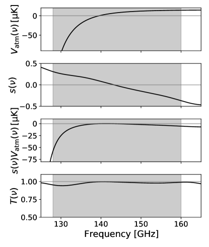
Figure 1: (Top) Brightness temperature spectrum of the atmospheric circular polarization signal. (Upper Middle) Spectrum of the conversion factor from $V$ to $U$ in conversion by the HWP. (Lower middle) Combination of the two effects. (Bottom) The transmittance of the HWP. The shaded region shows the averaged detector bandpass shown in Table 1.

2.2 Half-wave plate

Polarbear adopts a HWP to modulate the linear polarization signal. An ideal HWP does not convert the circular polarization to linear polarization. In practice, however, the ideal condition is satisfied only at a specific frequency, and non-zero conversion occurs at other frequencies in the observation frequency band. Using this non-ideality of the HWP, one can measure the circular polarization (Nagy et al., 2017).

The optical properties of the Polarbear HWP were measured in the laboratory before observations were made (Fujino et al., 2023). The conversion factor from the circular polarization (Stokes $V$) to linear polarization (Stokes $U$) is expressed as a parameter $s$ in the Mueller matrix:

$$\begin{pmatrix}I_{\mathrm{out}}(\nu)\\ Q_{\mathrm{out}}(\nu)\\ U_{\mathrm{out}}(\nu)\\ V_{\mathrm{out}}(\nu)\end{pmatrix}=\begin{pmatrix}T(\nu)&\rho(\nu)&0&0\\ \rho(\nu)&T(\nu)&0&0\\ 0&0&c(\nu)&-s(\nu)\\ 0&0&s(\nu)&c(\nu)\end{pmatrix}\begin{pmatrix}I_{\mathrm{in}}(\nu)\\ Q_{\mathrm{in}}(\nu)\\ U_{\mathrm{in}}(\nu)\\ V_{\mathrm{in}}(\nu)\end{pmatrix},$$ (1)

where $T(\nu)$, $\rho(\nu)$, and $c(\nu)$ are the transmittance, differential transmittance between the two HWP axes, and polarization efficiency, respectively. We calculate the spectrum of $s(\nu)$ following Essinger-Hileman (2013). The estimated spectrum of $s(\nu)$ is shown in Figure 1. $s(\nu)$ becomes zero around the band center and becomes positive and negative at lower and higher frequencies, respectively.

2.3 Simulation

We simulate the expected signal using the above models. The effective circular polarization signal $\overline{sV}$ is the product of the source spectrum $V(\nu)$ in brightness temperature units and $s(\nu)$ averaged over the detector bandpass function $W(\nu)$:

$$\overline{sV}=\frac{\int s(\nu)V(\nu)W(\nu)d\nu}{\int W(\nu)T(\nu)d\nu}\;.$$ (2)

In this calculation, the source spectrum is divided by the HWP transmittance $T(\nu)$ because the instrument is calibrated using thermal sources and the HWP transmittance is not included in $W(\nu)$. Moreover, we show the $T(\nu)$ spectrum in Figure 1.

We calculate the band-averaged $sV$ values at each of the seven detector wafers (see Section 3.1). Because of the strong frequency dependence on the atmospheric signal, the averaged $V$ is sensitive to the lower frequency edge of the bandpass. The bandpass function of Polarbear detectors is measured at the site (Matsuda et al., 2019, see also Section 3). The detector bandpass within a wafer is almost constant, whereas there is a slight difference between wafers. The integration range is twice the bandwidth above and below the center frequency. This range is roughly from $85\,\rm{GHz}$ to $205\,\rm{GHz}$. In the following sections, values without reference to $\nu$ are band-average values.

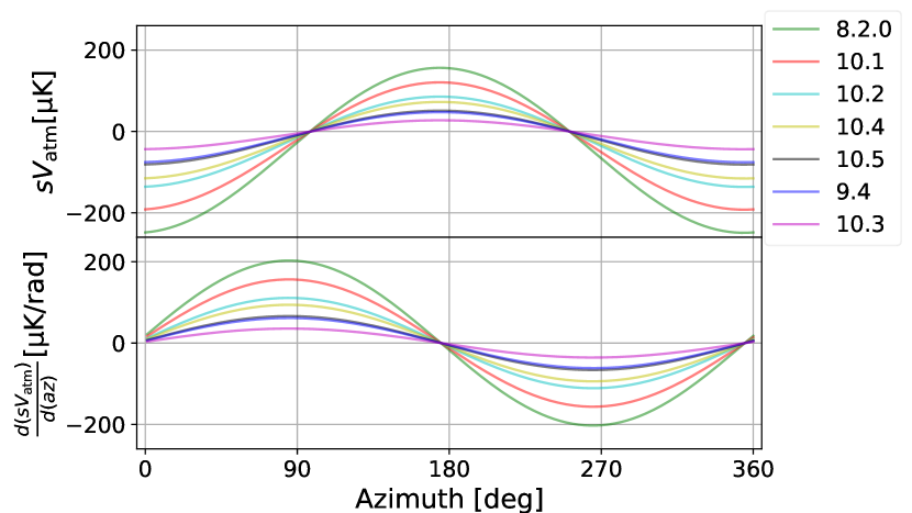
Figure 2: Azimuthal dependence of the $sV$ signal and its differential for the azimuthal angle. The elevation used in this simulation is 30 degrees. Each color represents the wafer on which the detectors are mounted. The legend on the right side of the plot is arranged in order of wafers, starting with those that have the lowest lower edge of the bandpass.

Figure 2 shows the simulated $sV$ signal for each wafer. The amplitudes of the cosine curve increase as the lower-edge frequency of the bandpass decreases. Figure 2 also shows the derivative of the $sV$ signal in terms of the azimuthal angle. The absolute value of the derivative has maximum values of $\sim 200\,\mathrm{\mu K/rad}$ around azimuthal angles of 90 and 270 degrees.

2.4 Circular polarization signal in the detector timestream

The expected detector signal is estimated by calculating the series of Mueller matrices of optical elements including the circular polarization component (Fujino et al., 2023). Using the dependence on the angle of the HWP, $\theta=\omega t$, the detector timestream is decomposed into three harmonics as:

$$d(t)=d_{0}(t)+d_{2}(t)+d_{4}(t)\;.$$ (3)

The unmodulated component $d_{0}(t)$ mainly contains the variation of the intensity signal as:

$$d_{0}(t)=\Delta I\;.$$ (4)

$d_{4}(t)$ is the component modulated by $4\theta$. The linear polarization signals (Stokes $Q$ and $U$ defined on the instrumental coordinate) appear in this component as:

$$d_{4}(t)=\mathrm{Re}[(Q+iU)\exp(4i\theta+2i\phi)]\;.$$ (5)

Here, the signal depends on the detector polarization angle $\phi$, which is defined as the angle on the instrument coordinates that the detector is sensitive to.

$d_{2}(t)$ is the component modulated by $2\theta$. It is calculated as:

$$\begin{split}d_{2}(t)=\mathrm{Re}[&(\rho I+isV)\exp(2i\theta+2i\phi)\\ &+\rho(Q+iU)\exp(2i\theta)]\;.\end{split}$$ (6)

Here, $\rho$ is the band-averaged $\rho(\nu)$. The first half of the expression corresponds to signals from the Stokes $I$ and $V$ converted to linear polarizations by the HWP. The second half corresponds to signals from the linear polarizations converted to unpolarized signals by the HWP, and it thus depends on $\theta$ but not $\phi$.

To extract signals, we demodulate the detector signal using the measured HWP angle $\tilde{\theta}$ and detector angle $\tilde{\phi}$. We obtain demodulated timestreams for each harmonic as:

$$\tilde{d}_{0}(t) =F_{\mathrm{LPF}}[d(t)]\approx\Delta I\;,$$ (7)

$$\tilde{d}_{4}(t) =F_{\mathrm{LPF}}\large[d(t)\cdot 2\exp(-4i\tilde{\theta}-2i\tilde{\phi})\large]$$

$$\approx Q+iU\;,$$ (8)

$$\tilde{d}_{2}(t) =F_{\mathrm{LPF}}\large[d(t)\cdot 2\exp(-2i\tilde{\theta}-2i\tilde{\phi})\large]$$

$$\approx\rho I+isV+\rho(Q+iU)\exp(-2i\tilde{\phi})\;,$$ (9)

where $F_{\mathrm{LPF}}$ is a low-pass filter used to extract the specified harmonic and exclude other harmonics. The intensity and linear polarization signals are obtained directly as $\tilde{d}_{0}(t)$ and $\tilde{d}_{4}(t)$. The circular polarization signal $sV$ is obtained from the imaginary part of $\tilde{d}_{2}(t)$, where the additional $\rho(Q+iU)$ term can be separated using the orthogonal detector.

In addition to this basic model, we consider various types of instrumental nonideality: the HWP synchronous signal, imperfections of other optical elements, variation in the detector time constant, and the effect of oblique incidence (Appendix A).

3 Instrument and data

3.1 Instrument

Polarbear is an experiment observing the CMB in the Atacama Desert in Chile. A cryogenic receiver (Arnold et al., 2012; Kermish et al., 2012) is installed on the Huan Tran Telescope with 2.5 m-aperture off-axis Gregorian optics. The HWP described in Section 2.2 is placed at the prime focus and is continuously rotated at 2.0 Hz during observations (Takakura et al., 2017). Before reaching detectors, light passes through a vacuum window, infrared filter, another cryogenic HWP, and three re-imaging lenses.

On the focal plane, there are seven wafers of the detector array cooled to 0.3 K. Each wafer comprises 182 transition-edge sensor bolometers with lenslet-coupled double-slot dipole antennas (Arnold et al., 2012). The observing frequency band is determined by bandpass filters in the antenna circuit and has small variations due to fabrication conditions. In this analysis, we use bandpass measurements made at the site using a Fourier transform spectrometer (FTS, Matsuda et al., 2019). The properties are listed in Table 1.

Table 1: Detector bandpass per wafer

Wafer	Band center	Band width	Lower edge
	[GHz]	[GHz]	[GHz]
8.2.0	136.9	30.4	121.7
10.1	142.1	31.8	126.2
10.2	143.5	32.6	127.2
10.4	144.0	32.2	127.9
10.5	145.5	31.8	129.6
9.4	146.9	32.8	130.5
10.3	148.7	31.0	133.2

Note. — From Matsuda et al. (2019)

3.2 Observations

Polarbear made observations from January 2012 to January 2017. In this analysis, we use 3 years of observational data covering a 670-square-degree patch obtained using the continuously rotating HWP, starting in July 2014. This data set is the same used by Polarbear Collaboration (2022, PB22 hereafter), encompassing the third, fourth, and fifth seasons listed in Table 3.

As described in Polarbear Collaboration (2020, PB20 hereafter), the scan strategy adopts three sets of scan directions—rising, middle, and setting scans—to follow the sky rotation. In each scan direction, we perform a set of right-going and left-going constant elevation scans at a scan speed of $0.4\arcdeg/\mathrm{s}$ on the sky. The scan ranges are listed in Table 2. The elevation of the middle scan is stepped each day. The duration of one observation is approximately 1 hour.

Table 2: Properties of scan directions

			Number of
Name	Azimuth range	Elevation	observations
Rising
r	[$133\arcdeg$, $156\arcdeg$]	$30.0\arcdeg$	1042
Middle
m0	[$154\arcdeg$, $206\arcdeg$]	$45.5\arcdeg$	93
m1	[$154\arcdeg$, $206\arcdeg$]	$47.7\arcdeg$	107
m2	[$154\arcdeg$, $206\arcdeg$]	$50.0\arcdeg$	104
m3	[$150\arcdeg$, $209\arcdeg$]	$52.2\arcdeg$	148
m4	[$150\arcdeg$, $209\arcdeg$]	$54.4\arcdeg$	132
m5	[$145\arcdeg$, $214\arcdeg$]	$56.6\arcdeg$	118
m6	[$145\arcdeg$, $214\arcdeg$]	$58.9\arcdeg$	116
m7	[$145\arcdeg$, $214\arcdeg$]	$61.1\arcdeg$	94
m8	[$138\arcdeg$, $222\arcdeg$]	$63.3\arcdeg$	148
m9	[$138\arcdeg$, $222\arcdeg$]	$65.5\arcdeg$	120
Setting
s	[$202\arcdeg$, $227\arcdeg$]	$35.2\arcdeg$	1471

3.3 Data selection

The data selection in this analysis is based on that of PB22. In this data selection, we establish thresholds and eliminate bad data, including readings from detectors with no optical response or no calibration data, timestreams having high noise levels, scans containing glitches, and observations made during poor weather. In addition to the selection criteria of PB22, we discard 9.5% of observations that have outlier slope values in the circular polarization signal estimates described below.

Table 3: Number of 1-hour observations

				PWV	PWV
Season	Total	Daytime	Night
				$<$1 mm	$\geq$1 mm
Third season	943	196	747	564	379
Fourth season	1453	413	1040	875	578
Fifth season	1297	314	983	824	473

4 Analysis

The atmospheric circular polarization signal is expected to have cosine-like variation as a function of the azimuth angle (Figure 2, top). As the range of Polarbear scans (Table 2) is limited, only a small part of the cosine curve is observed, which should appear as a slope, depending on the azimuth (Figure 2, bottom). We measure the difference in the slope across different scan directions. As shown in Figure 2, we expect the slope for the middle direction to be small. We thus use the slopes of the rising and setting directions for the quantitative evaluation and use the slope of the middle direction for demonstration and validation purposes. Finally, we evaluate the dependence on the detector bandpass (Table 1) in simulation (Section 2.3) to confirm the signature of the strong frequency dependence in the atmospheric circular polarization signal shown in Figures 1 and 2.

The challenge in our analysis is to control the contamination of ground-synchronous signals leaking from $I$, $Q$, and $U$ parameters. As shown later, we find that this systematic error can be appreciably larger than the atmospheric circular polarization signal. However, through the polarization modulation described in Section 2.4, we can separately obtain other Stokes parameters, $I$, $Q$, and $U$, and subtract the ground contamination from the circular polarization signal. Here, we assume that the atmospheric circular polarization signal is constant over the 3 years of observations, whereas the ground-synchronous signal may vary owing to activities at the site, such as the construction of the Simons Array, which involves upgrading the experiment to include two telescopes to the north and south of the Polarbear telescope. Moreover, we assume that the ground-synchronous signal is not circularly polarized.

4.1 Calibration and preprocessing

Calibrations are based on those of PB20 and PB22. Here, we describe differences for the circular polarization measurement. As shown in Section 2.4, the circular polarization signal has a dependence of $(\theta+\phi)$, whereas the calibration of the polarization angle calibrates the linear combination of $(2\theta+\phi)$. We therefore calibrate the HWP angle $\theta$ independently from the linearly polarized astronomical source measurements with and without the HWP. We also conduct an additional calibration of polarization efficiency. We consider the contributions of the secondary mirror and the cryogenic HWP and estimate the polarization efficiency to be 92%. We ignore the pointing offset of each detector and the beam effect because the atmospheric circular polarization signal varies over a scale larger than the focal plane field of view.

Each detector timestream is calibrated to Rayleigh–Jeans temperature units using a thermal source calibrator, whose effective temperature is calibrated by Jupiter observations. Unlike PB20 and PB22, the overall calibrations made using the CMB power spectrum are not applied because the source spectrum is different from CMB. The effect of the detector time constant is corrected by deconvolving the time constant. The calibrated timestream is demodulated and downsampled using the encoded angle of the rotating HWP. Here, we extract the second harmonic, $\tilde{d}_{2}(t)$, in addition to the zeroth and fourth harmonics, $\tilde{d}_{0}(t)$ and $\tilde{d}_{4}(t)$. The demodulated timestreams are filtered by second-order polynomials over the 1-hour observation to remove slow variations that are mainly caused by variation in the focal plane temperature. In contrast to PB22, the scan-by-scan polynomial filter is not applied in this analysis.

Next, we average detector timestreams wafer-by-wafer and decompose them into components. Following Equation 9, the second harmonic demodulated timestream of the $i$-th detector is modeled as:

$$\tilde{d}_{2,i}(t)\approx\rho I+isV+\rho(Q+iU)\exp(-2i\tilde{\phi}_{i})\;,$$ (10)

where $\tilde{\phi}_{i}$ is the detector polarization angle. We solve this equation by averaging multiple detectors with different polarization angles as:

$$\begin{split}&\left[\begin{matrix}\rho I&sV&\rho Q&\rho U\end{matrix}\right]^{\mathsf{T}}\approx\left[\begin{matrix}\tilde{d}^{(2,2,\mathrm{Re})}(t)&\tilde{d}^{(2,2,\mathrm{Im})}(t)&\tilde{d}^{(2,0,\mathrm{Re})}(t)&\tilde{d}^{(2,0,\mathrm{Im})}(t)\end{matrix}\right]^{\mathsf{T}}\\ &=\left[\begin{matrix}\sum_{i}w_{i}&0&\sum_{i}w_{i}\cos 2\tilde{\phi}_{i}&\sum_{i}w_{i}\sin 2\tilde{\phi}_{i}\\ 0&\sum_{i}w_{i}&\sum_{i}-w_{i}\sin 2\tilde{\phi}_{i}&\sum_{i}w_{i}\cos 2\tilde{\phi}_{i}\\ \sum_{i}w_{i}\cos 2\tilde{\phi}_{i}&\sum_{i}-w_{i}\sin 2\tilde{\phi}_{i}&\sum_{i}w_{i}&0\\ \sum_{i}w_{i}\sin 2\tilde{\phi}_{i}&\sum_{i}w_{i}\cos 2\tilde{\phi}_{i}&0&\sum_{i}w_{i}\end{matrix}\right]^{-1}\cdot\left[\begin{matrix}\sum_{i}w_{i}\mathrm{Re}[\tilde{d}_{2,i}(t)]\\ \sum_{i}w_{i}\mathrm{Im}[\tilde{d}_{2,i}(t)]\\ \sum_{i}w_{i}\mathrm{Re}[\tilde{d}_{2,i}(t)\exp(2i\tilde{\phi}_{i})]\\ \sum_{i}w_{i}\mathrm{Im}[\tilde{d}_{2,i}(t)\exp(2i\tilde{\phi}_{i})]\end{matrix}\right].\end{split}$$ (11)

Here, the weights $w_{i}$ are calculated using the inverse variance of the detector white noise. The detector angle $\phi_{i}$ distributes across four angles every $\pi/4$ such that the weight matrix is nearly diagonal. These timestreams are summed over the detector index $i$ within a wafer so that the timestreams $d^{(*)}(t)$ are wafer-averaged values. The superscript of the decomposed timestreams, such as ${(2,2,\mathrm{Re})}$, shows the dependencies on the HWP angle, detector polarization angle, and real or imaginary component (see, e.g., Equation 6). The circular polarization signal is extracted from the $(2,2,\mathrm{Im})$ component as:

$$\tilde{d}^{(2,2,\mathrm{Im})}(t)\approx sV\;.$$ (12)

Equation 11 shows decomposition into four components. However, we can consider more components with a different dependence on the detector polarization angle $\phi$. Such extra components can be introduced by systematic effects of the instruments, such as intensity-to-polarization leakage in the optics and detector nonlinearity. We separate these systematic effects by extending the components for decomposition in the averaging method and reduce their contamination into the signal components used in the following analysis. In practice, we decompose the zeroth, second, and fourth harmonics into three, eight, and eight components, respectively. See Appendix A for more details.

Note that the decomposed timestreams may contain systematic leakages from other modes. We estimate the leakage coefficients and subtract them at a later stage, as described in Section 4.3.

4.2 Estimation of the azimuthal slope

The atmospheric circular polarization signal is expected to follow a sinusoidal pattern as a function of azimuth. We fit each component of the averaged timestreams, $\tilde{d}^{(*)}(t)$, with a polynomial function of the telescope azimuth, $a(t)$, by minimizing:

$$\sum_{t}w_{\mathrm{scan}}\Big{[}\tilde{d}^{(*)}(t)-\sum_{i=0}^{2}p_{i,\mathrm{obs}}^{(*)}\,\{\Delta a(t)\}^{i}\Big{]}^{2}\;,$$ (13)

where the per-subscan weight $w_{\mathrm{scan}}=\sum_{i}w_{i}$ is the total weight summed over detectors, $\Delta a(t)=a(t)-a_{0}$ is the azimuth offset from the scan center $a_{0}$, and $p_{i,\mathrm{obs}}^{(*)}$ denotes each of the polynomial coefficients. $p_{1,\mathrm{obs}}^{(2,2,\mathrm{Im})}$ corresponds to the azimuthal slope of the atmospheric circular polarization signal, $sV$.

We then take the average of slopes from many observations for each scan direction, $d\in(\rm{r,m,s})$, and each wafer. To correct for leakage systematics in each season, we perform averaging in two steps. First, we compute the average of the slope value $p_{1,d,y}^{(*)}$ for each season, $y\in(3,4,5)$, with the inverse-variance weight of $w_{\rm{obs}}=\sum_{\mathrm{scan}}w_{\mathrm{scan}}$. We then compute the inverse-variance weighted average among seasons, $p_{1,d}^{(*)}$, using the statistical error (Section 4.4) and the systematic error of the leakage subtraction (Section 4.4.2).

We also estimate the azimuthal slope of the atmospheric circular polarization signal for each wafer and each scan direction using the simulation results(Section 2.3). We test their consistency by taking the ratio of the measured value to the simulation value.

4.3 Leakage subtraction

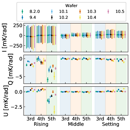
Figure 3: Measured azimuthal slopes of the intensity and linear polarization signals for each wafer, season, and scan direction. The points show median values and the error bars show observation-by-observation variation. The linear polarization signals shown are those after subtraction of the intensity leakage.

Leakages of intensity and linear polarization into circular polarization estimates are some of the most concerning sources of systematic error. We subtract measurements of these leakages in our analysis.

We consider linear leakages from the intensity and linear polarization signals expressed as:

$$\tilde{d}^{(2,2,\mathrm{Im})}(t)=sV+\lambda^{I\rightarrow sV}I+\lambda^{Q\rightarrow sV}Q+\lambda^{U\rightarrow sV}U\>,$$ (14)

where $\lambda^{X\to Y}$ is the leakage coefficient from each component $X$ to $Y$. Expressions of the leakage coefficients based on the instrumental model are explained in Appendices A and B. As intensity and linear polarization signals have large variations among seasons and non-zero values of the azimuthal slope as shown in Figure 3, their leakages may increase the uncertainty in the circular polarization measurements and bias the results. We assume that the variation in the intensity signal is due to atmospheric variation and that the variation in the linear polarization signal comes from the far sidelobe pickup of containers and site activities.

To minimize these systematic errors, we subtract the leakages using the observed $I$, $Q$, and $U$ signals. We first approximate Equation 14 by:

$$\begin{split}\tilde{d}^{(2,2,\mathrm{Im})}(t)\approx sV&+\tilde{\lambda}^{I\rightarrow sV}\tilde{d}^{(0,0,\mathrm{Re})}\\ &+\tilde{\lambda}^{Q\rightarrow sV}(\tilde{d}^{(4,2,\mathrm{Re})}-\tilde{\lambda}^{I\rightarrow Q}\tilde{d}^{(0,0,\mathrm{Re})})\\ &+\tilde{\lambda}^{U\rightarrow sV}(\tilde{d}^{(4,2,\mathrm{Im})}-\tilde{\lambda}^{I\rightarrow U}\tilde{d}^{(0,0,\mathrm{Re})})\;,\end{split}$$ (15)

where $\tilde{\lambda}^{X\rightarrow Y}$ is the coefficient of leakage from component $X$ to $Y$, which we estimate from the observation data. We then subtract the leakages by scaling the source signal $X$. Here, we assume that the variation in the atmospheric circular polarization signal for each scan direction should be small and that all variations correlated with the source signals are due to the leakages. We thus estimate the leakage coefficients such that the variance of the circular polarization signal after the leakage subtraction is minimized. In addition, we assume that this leakage subtraction removes the bias. Here, we briefly describe the methods and results. Further details and discussions are presented in Appendix B.

We first estimate the coefficient of leakage from the intensity signal, specifically the $(0,0,\mathrm{Re})$ component. We estimate the leakage coefficients for every 1-hour observation using the correlation of the wafer-averaged timestreams $\tilde{d}^{(*)}(t)$ and subtract the scaled template of the $(0,0,\mathrm{Re})$ component from the other components. After this leakage subtraction, the variation in the slope $p_{1,\mathrm{obs}}^{(2,2,\mathrm{Im})}$ decreases in all wafers except wafer 10.1. In particular, the standard deviation decreases by approximately 90% in wafer 10.2. Moreover, the coefficient of correlation between $p_{1,\mathrm{obs}}^{(0,0,\mathrm{Re})}$ and $p_{1,\mathrm{obs}}^{(2,2,\mathrm{Im})}$ decreases to $<7\%$ in all wafers. In addition, the coefficient of correlation between $p_{1,\mathrm{obs}}^{(2,2,\mathrm{Im})}$ and the leakage coefficient of this intensity subtraction is $<10\%$. Therefore, the systematic error due to the leakage of the intensity signal is well subtracted, and the residual should have a subdominant effect.

We then estimate the coefficients of leakage from the linear polarization, $(4,2,\mathrm{Re})$ and $(4,2,\mathrm{Im})$. We estimate the leakage coefficients for each scan direction over all seasons to minimize the variance in the slope of the circular polarization signal $p_{1,\mathrm{obs}}^{(2,2,\mathrm{Im})}$ after subtracting scaled $p_{1,\mathrm{obs}}^{(4,2,\mathrm{Re})}$ and $p_{1,\mathrm{obs}}^{(4,2,\mathrm{Im})}$. After this leakage subtraction, the standard deviation of the slope $p_{1,\mathrm{obs}}^{(2,2,\mathrm{Im})}$ decreases by approximately $10\%$ in wafer 8.2.0 and $80\%$ in wafer 10.4.

4.4 Error estimation

Table 4: List of uncertainties and correlations assumed

	Correlated	Correlated	Correlated
	among	among	among
Type of uncertainty	directions	wafers	seasons
Measurement
Statistical error
Systematic error of linear polarization leakage subtraction
Excess seasonal variation
Systematic error of angle calibration			$\checkmark$
Systematic error of absolute gain	$\checkmark$	$\checkmark$	$\checkmark$
Systematic error of polarization efficiency	$\checkmark$		$\checkmark$
Simulation
Systematic error of bandpass uncertainty	$\checkmark$		$\checkmark$
Systematic error of the HWP	$\checkmark$	$\checkmark$	$\checkmark$
Systematic error of temporal variation of the signal	$\checkmark$	$\checkmark$	$\checkmark$

We estimate the uncertainties in both the measured and simulated values of the azimuthal slope of the atmospheric circular polarization signal for each wafer and scan direction. The uncertainties are summarized in Table 4.

For the uncertainties in the measurements, we consider the statistical uncertainty, the systematic uncertainties due to the leakage subtraction, the uncertainty in the polarization angle, the uncertainties in the absolute gain and polarization efficiency, and the extra-seasonal variations. For the uncertainties in the simulation, we consider systematic uncertainties relating to the detector bandpass, the temporal variation in the atmospheric circular polarization, the uncertainty in the atmospheric model, and the uncertainty in the HWP model.

We estimate the measurement uncertainties in two steps as performed in Section 4.2. We first estimate the uncertainty for each season, including the statistical uncertainty, the systematic uncertainty in the leakage subtraction, and the extra-seasonal variation. We then estimate the uncertainty in the average among seasons and add other systematic uncertainties in quadrature.

We consider that all simulation uncertainties are multiplicative. Therefore, we estimate fractional uncertainties relative to the simulation value for each source and take their quadratic sum.

Finally, the uncertainty in the ratio of the measurement to the simulation for each wafer and direction is estimated through the error propagation of both uncertainties. The uncertainty in the ratio averaged over wafers and directions is also calculated through the error propagation considering the correlations as shown in Table 4.

4.4.1 Statistical uncertainty

We estimate the statistical uncertainty for each wafer and scan direction $d$ for each season $y$ using the sign-flip method. We calculate:

$$p_{1,d,y,\mathrm{sf}}^{(2,2,\mathrm{Im})}=\frac{\sum_{\mathrm{obs}\in(d,y)}f_{\mathrm{obs}}w_{\mathrm{obs}}p_{1,\mathrm{obs}}^{(2,2,\mathrm{Im})}}{\sum_{\mathrm{obs}\in(d,y)}w_{\mathrm{obs}}}\;,$$ (16)

where the set of random values $f_{\mathrm{obs}}=\{1$ or $-1\}$ is realized many times such that $\sum_{\mathrm{obs}\in(d,y)}w_{\mathrm{obs}}f_{\mathrm{obs}}\sim 0$. The standard deviation of the results is then taken. Here, $p_{1,\mathrm{obs}}^{(2,2,\mathrm{Im})}$ is calculated after the leakage subtractions.

4.4.2 Systematic uncertainty in leakage subtraction

Leakage subtractions with wrong estimations of the leakage coefficients, $\tilde{\lambda}^{I\to sV}$, $\tilde{\lambda}^{Q\to sV}$, and $\tilde{\lambda}^{U\to sV}$ may introduce systematic error.

For the leakage from intensity, owing to the large signal from atmospheric fluctuation, we can accurately estimate the leakage coefficient for each observation, and the cause of its variation is detector nonlinearity (Appendix B.1). We thus assume that this systematic error is negligible. This is supported by an analysis of correlation between $p_{1,\mathrm{obs}}^{(2,2,\mathrm{Im})}$ and the intensity leakage coefficient in Section 4.3, which is sensitive to this systematic error.

For leakage from linear polarization, the source of the leakage and its variations are not fully understood. We estimate the statistical uncertainty in the measured leakage coefficient using the bootstrap method. In addition, we estimate the systematic uncertainty in the leakage coefficients as the seasonal variations in the leakage estimates (See Figure 10). To account for the seasonal variation in the linear polarization signals shown in Figure 3, we evaluate the systematic error for each season and direction as:

$$\begin{split}&\left[\left(\tilde{\lambda}^{Q\to sV}\delta p_{1,d,y,\mathrm{stat}}^{(4,2,\mathrm{Re})}\right)^{2}+\left(\tilde{\lambda}^{U\to sV}\delta p_{1,d,y,\mathrm{stat}}^{(4,2,\mathrm{Im})}\right)^{2}\right.\\ &\left.+\left(\delta\tilde{\lambda}^{Q\to sV}_{\mathrm{stat}}p_{1,d,y}^{(4,2,\mathrm{Re})}\right)^{2}+\left(\delta\tilde{\lambda}^{U\to sV}_{\mathrm{stat}}p_{1,d,y}^{(4,2,\mathrm{Im})}\right)^{2}\right.\\ &\left.+\left(\delta\tilde{\lambda}^{Q\to sV}_{\mathrm{sys}}p_{1,d,y}^{(4,2,\mathrm{Re})}\right)^{2}+\left(\delta\tilde{\lambda}^{U\to sV}_{\mathrm{sys}}p_{1,d,y}^{(4,2,\mathrm{Im})}\right)^{2}\right]^{1/2}\;.\end{split}$$ (17)

Because of the seasonal variation in the linear polarization signals, we assume that this error is uncorrelated among wafers, directions, and seasons. The final systematic uncertainty of leakage subtraction for each wafer and scan direction is estimated from the error propagation in averaging among seasons, which is approximately 10% of the signal amplitude.

4.4.3 Excess systematic variation among seasons

We incorporate an additional systematic uncertainty for seasonal variations specific for each wafer and scan direction. This uncertainty is adjusted so that the reduced chi-squared of the average among seasons becomes unity if the original residual chi-squared exceeds unity. Here, we assume that this error is uncorrelated among seasons. This procedure is applied to wafers 8.2.0 and 10.1, which are expected to see larger signals of atmospheric circular polarization and might be more sensitive to multiplicative systematic uncertainties.

4.4.4 Polarization angle uncertainty

Our linear polarization angle calibration follows PB20, with an associated uncertainty of $0.22^{\circ}$, which is negligibly small for this analysis. This calibration determines the linear combination of $2\tilde{\theta}+\tilde{\phi}$ whereas, as described in Section 4.1, the circular polarization signal depends on $\theta+\phi$. We thus need to estimate the HWP angle $\tilde{\theta}$ independently from the angle calibration. The absolute value, or the calibrated zero point of $\tilde{\theta}$, contains a systematic error. This angular error affects the phase of the demodulated signals and contaminates the intensity leakage signal $\rho I$ into the circular polarization signal $sV$, as described by:

$$\begin{split}\tilde{d}^{(2,2,\mathrm{Re})}&\approx\rho I\cos 2\Delta-sV\sin 2\Delta\;,\\ \tilde{d}^{(2,2,\mathrm{Im})}&\approx sV\cos 2\Delta+\rho I\sin 2\Delta\;,\end{split}$$ (18)

where $\Delta=\tilde{\theta}-\theta$ is the absolute angular error of the HWP.

We evaluate $\Delta$ using the polarized second harmonic of the HWP synchronous signal (2f HWPSS): i.e., $p_{0,\mathrm{obs}}^{(2,2,\mathrm{Re})}$ and $p_{0,\mathrm{obs}}^{(2,2,\mathrm{Im})}$ in Equation 13. As described in the optical model of the HWP in Section 2.2, the main sources of the polarized 2f HWPSS are the differential transmission, reflection, and emission of the HWP, as well as the circular polarization signal, $sV$. In an ideal case, the circular polarization signal appears in the imaginary part of the polarized 2f HWPSS, $p_{0,\mathrm{obs}}^{(2,2,\mathrm{Im})}$, and differential transmission, reflection, and emission of the HWP appear in the real part, $p_{0,\mathrm{obs}}^{(2,2,\mathrm{Re})}$, but the angular error may rotate these phases. Among these, we expect that the variation in the differential transmission ($\rho I$) is the largest owing to the variation in the observation weather. We thus can estimate the potential angular error $\Delta$ by performing the principal component analysis on the $2\Delta$-rotated slopes of the 2f HWPSS to determine the phase that maximizes the variation in the $\rho I$ term.

We estimate this phase rotation of the polarized 2f signal for each wafer, scan direction, and season. We find that there are systematic variations in the phase rotation of the polarized 2f signal ($2\Delta$) from $0\arcdeg$ to $8\arcdeg$. Therefore, we estimate the systematic 2f-phase uncertainty $2\delta\Delta=4\arcdeg$ and the systematic uncertainty in the circular polarization signal as $2|\tilde{p}^{(2,2,\mathrm{Re})}_{1,d}|\delta\Delta$. To be conservative, we take the maximum value among directions for each wafer and treat this uncertainty as being uncorrelated among directions and wafers. The corresponding systematic uncertainties in the slope of the $sV$ signal are from 10% to 60% of the signal.

4.4.5 Absolute gain and polarization efficiency

Here, we consider multiplicative uncertainties in the measurements. We use the same absolute gain value used in the linear polarization observation (PB20), which is calibrated by planet observations. The fractional uncertainty of the absolute gain calibration is approximately 2%. We assume this error is correlated among all wafers and directions.

The polarization efficiency also has uncertainty. We estimate this uncertainty from the variation due to the detector position and the difference between wafers due to the bandpass difference. This fractional uncertainty is approximately 5%. We assume this error is uncorrelated among wafers.

4.4.6 Bandpass uncertainty

There could be uncertainty in the bandpass measurement (Matsuda et al., 2019) causing a systematic error in the band average, Equation 2. We evaluate the uncertainty due to the variation in the detector response within the wafer as follows. First, we generate 5000 random realizations of the bandpass for each wafer using the bootstrap method. We then calculate the slope of the band-averaged $sV$ following the same approach as in Section 2.3 using a bandpass that includes this noise and take the standard deviation among the realizations as the uncertainty in the signal. The fractional uncertainty is at the level of a few percent.

We also assume that the bandpass measurement contains a systematic error in frequency scaling. To evaluate the effect of this frequency uncertainty, we calculate the slopes of the $sV$ signal by scaling the frequency of the bandpass and compare them with the value obtained without scaling. We define the systematic error as the maximum slope difference observed when varying the frequency within the $1\,\mathrm{GHz}$ frequency resolution of the FTS measurement. These fractional uncertainties are typically 8%, and 14% in the worst case.

We assume these errors are correlated among directions but not among wafers because they depend on the shape of the bandpass and possibly on the position on the focal plane.

4.4.7 HWP model uncertainty

The HWP model contains uncertainty. We previously estimated in Fujino et al. (2023) that the uncertainty in the HWP leakage parameter $s$ is less than 3%.

4.4.8 Temporal variation in the atmospheric circular polarization signal

The direction and amplitude of Earth’s magnetism change year by year. In the simulation, we calculate the expected atmospheric circular polarization using the direction and amplitude of Earth’s magnetism in the middle of the observation period using the enhanced magnetic model 2015 (EMM2015, Chulliat, 2015). To estimate the effects of the temporal variation of Earth’s magnetism on the slope, we calculate the direction and amplitude of Earth’s magnetism at the beginning, middle, and end of the observation period. The fractional difference in the amplitude is 1% and the difference in the direction is approximately $0.5^{\circ}$ in this period. The impact of the temporal variation in Earth’s magnetism on the slope of $sV$ is approximately 5% in the middle direction, less than 2% in the rising direction, and less than 1% in the setting direction. This dependence on the observation direction comes from the variation in the direction of Earth’s magnetism. The effect on the middle direction is relatively pronounced owing to the small slope values. However, we use the slopes in the middle direction as a reference only and do not use them in the evaluation, rendering this a minor effect.

Moreover, we consider temperature and pressure to be time-varying parameters. The standard deviation of the pressure observed at the Polarbear site is less than 1% relative to the average, and the effect on the slope values is 1% or less. The seasonal temperature variation is typically $\sim 30\,\rm{K}$ at the observation site. According to Table 5 in Spinelli et al. (2011), the effect of temperature variation on Zeeman emission is less than $3\,\rm{\mu K}$, which corresponds to 5% of the signal. Furthermore, we assume this does not create azimuthal variation. Therefore, we can confidently disregard this systematic effect.

4.4.9 Atmospheric emission model uncertainty

P20 found discrepancies of $\sim 20\%$ in signal amplitude between data and simulation. It was concluded that this is due to simulation inaccuracy of the atmospheric spectrum frequencies away from the oxygen resonance line. In our case, as we observed the signal close to the resonance line, this effect is considered to be less than 20%.

4.5 Validation

We validate the estimated azimuthal slopes of the circular polarization component by comparing the results obtained from subsets of data. We consider six subsets for the right-going scan, left-going scan, high precipitable water vapor ($\mathrm{PWV}>1\,\mathrm{mm}$), low PWV ($\mathrm{PWV}\leq 1\,\mathrm{mm}$), daytime, and night. In the scan direction splits, we test systematic errors due to the variation in the focal plane temperature. In the PWV splits, we can examine systematic errors arising from intensity leakage or variations in the time constant. In the daytime and night splits, we can investigate systematic errors related to ground temperature variations or far sidelobe observations of the Sun.

In the scan direction splits, we subtract the intensity leakage subtraction and estimate the azimuthal slope for each observation using the corresponding scans. In the other splits, we use the same coefficients of intensity leakage as used in the main analysis for each subset of observations. We use the same coefficients of linear polarization leakage as used in the main analysis for all cases. We use the measurement uncertainty estimated from all data including the statistical uncertainty and the systematic uncertainties from leakage subtraction, excess seasonal variations, and polarization angle uncertainty.

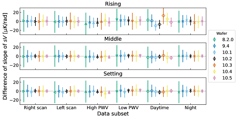
Figure 4: Deviation of measurements obtained from each subset of data relative to the full data analysis. Panels from top to bottom show values for rising, middle, and setting scan directions. The color of the points denotes the wafer and the symbol of the points indicates the subset of data.

Figure 4 shows the results. All points fall within $0.9\sigma$ of zero. We thus conclude that the slopes from all subsets align with the full data analysis, and there are no appreciable systematic uncertainties.

5 Results

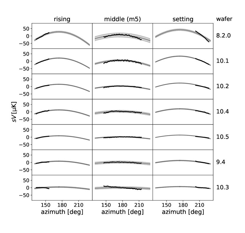
Figure 5: Binned azimuthal profiles for all wafers and scan directions (black points). Average values have been subtracted. Simulated $sV$ values are overlaid (gray lines). The gray bands show roughly estimated one-sigma regions obtained as half of the root sum square of errors in Table 5 times the azimuthal range. Note that there is an outlier for the setting direction, but the weight of this point is low and the effect on the calculation of the azimuthal slope is negligible. Therefore, we do not show this point.

Figure 5 shows binned azimuthal profiles overlaid with the simulated values. The data points in the rising and setting directions have a positive and negative azimuthal dependence as expected. Moreover, we find that data points in the middle direction peak around an azimuth of 180 degrees. The data points have an azimuthal dependence similar to that in the simulation. However, some wafers and directions display slope shapes slightly different from those in the simulation. The row of panels is ordered by the lower edge of the bandpass, and we see that a higher the lower edge of the bandpass corresponds to a smaller amplitude of the sinusoidal shape. Furthermore, we show roughly estimated errors as the shaded regions in Figure 5. These errors are calculated as the azimuthal range times half of the root sum square of all errors estimated in Section 4.4. It is seen that almost all of the data points in the rising and middle directions are within these bands.

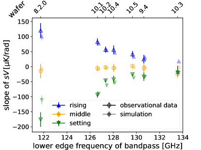
Figure 6: Slope of the apparent circular polarization signal versus the lower passband frequency of each wafer. Both observational and simulation data are shown.

Table 5: Slope values, observational data/simulation data ratios, and statistical error calculated in Section 4. All slope values are in units of $\rm{\mu K/rad}$.

		Wafer
		8.2.0	9.4	10.1	10.2	10.3	10.4	10.5
Azimuthal slope	rising	$120.4$	$25.0$	$82.9$	$56.9$	$-16.5$	$56.4$	$41.6$
of observational data	setting	$-175.9$	$-33.5$	$-93.9$	$-46.4$	$-19.6$	$-42.8$	$-25.8$
Azimuthal slope	rising	$99.7$	$30.3$	$76.9$	$54.6$	$17.5$	$46.3$	$32.6$
of simulation	setting	$-110.5$	$-34.0$	$-90.1$	$-61.9$	$-20.0$	$-53.2$	$-37.0$
Observational data/simulation	rising	$1.21\pm 0.02$	$0.82\pm 0.09$	$1.08\pm 0.03$	$1.04\pm 0.08$	$-0.95\pm 0.17$	$1.22\pm 0.12$	$1.28\pm 0.13$
data and statistical error	setting	$1.59\pm 0.01$	$0.99\pm 0.02$	$1.04\pm 0.01$	$0.75\pm 0.01$	$0.98\pm 0.06$	$0.81\pm 0.02$	$0.70\pm 0.02$

Table 6: List of errors in the averaged ratio.

Type of uncertainty	Value
Statistical error	$0.01$
Systematic error in	$0.01$
linear polarization leakage subtraction
Excess seasonal variation	$0.02$
Systematic error in angle calibration	$0.05$
Systematic error in absolute gain	$0.02$
Systematic error in polarization efficiency	$0.02$
Systematic error in bandpass uncertainty	$0.04$
Systematic error related to the HWP	$0.03$
Systematic error in temporal variation of the signal	$<0.01$
Atmospheric emission model uncertainty	$\ll 0.20$

We summarize the results of the azimuthal slope of the circular polarization signal $sV$ for each wafer and scan direction in Figure 6 and Table 5. We find a signal in both rising and setting observations, with the expected opposite signs. The amplitude of the signal is typically 20–100$\,\mathrm{\mu K/rad}$ depending on the lower edge of the passband frequencies. Moreover, Figure 6 shows the azimuthal slope derived from simulation. The estimated slopes are mostly consistent with the simulation results, particularly in terms of how their signs depend on azimuth and how their amplitudes relate to the wafers’ bandpass. However, there are discrepancies, which are discussed below.

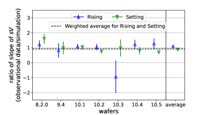
Figure 7: Ratio of the slope of $sV$ obtained from observational data to that obtained in simulation for each wafer in rising and setting directions. Also shown are the individual weighted-average values for each scan direction (at the right end), and the overall weighted-average value (the black dashed line).

We calculate the ratio of the slope values between data and simulation for each wafer in each of the rising and setting directions (Figure 7). We also show the weighted average over all wafers for each direction. The chi-squared values for the weighted average of these ratios for the rising and setting directions are 6.7 and 7.0, respectively, with six degrees of freedom. These chi-squared values correspond to p-values of 35% and 32%, respectively. The resultant averages of the data-to-simulation ratio of the slope are $1.09\pm 0.02\mathrm{(stat)}\pm 0.11\mathrm{(sys)}$ and $0.88\pm 0.01\mathrm{(stat)}\pm 0.08\mathrm{(sys)}$ in rising and setting directions, respectively.

We then average the ratio for the rising and setting directions. We show the statistical and systematic errors in this averaging in Table 6. The chi-squared in the averaging is 14.3 for 13 degrees of freedom, and the p-value is 35%. The average is $0.92\pm 0.01\mathrm{(stat)}\pm 0.07\mathrm{(sys)}$.

6 Conclusion

In this paper, we reported the observations of atmospheric circular polarization at $150\,\rm{GHz}$ using Polarbear data obtained using a continuously rotating HWP. The signs of slopes were opposite in the rising and setting directions, as expected. We found the largest slope of $120.4\pm 2.4\mathrm{(stat)}\pm 25.1\mathrm{(sys)}\,\rm{\mu K/rad}$ (rising) and $-175.8\pm 1.4\mathrm{(stat)}\pm 25.8\mathrm{(sys)}\,\rm{\mu K/rad}$ (setting) for the detectors on wafer 8.2.0, which had the lowest lower edge of the frequency bandpass. We also found a dependence on the small shift of the detector bandpass. These results showed that we could detect the atmospheric circular polarization signal using the leakage of the continuously rotating HWP. We compared these values with the results of simulation. We found consistency in the bandpass and scan direction dependencies between the observational data and simulation. We took the ratio of the slopes between data and simulation. The average of the overall wafer ratio, in both the rising and setting directions, was $0.92\pm 0.01\mathrm{(stat)}\pm 0.07\mathrm{(sys)}$ with a p-value of 35%. This result confirmed the validity of the simulation model based on the theory of atmospheric emission. In future investigations, we will need to better calibrate the absolute angle of the HWP and the absolute frequency of the bandpass measurement.

Although this study focused on measuring atmospheric circular polarization, our findings will be valuable in studying cosmological circular polarization by demonstrating the methodology involved. This work demonstrated the measurement of circular polarization using the HWP imperfections, which convert the circular polarization signal into the imaginary part of the second harmonic signal at the HWP rotation frequency. This analysis methodology is suitable for searching for a cosmological circular polarization signal. The polarization modulation technique using a rotating HWP is currently being widely adopted and will continue to be used in future CMB experiments, including the Simons Array and Simons Observation experiments (Hill et al., 2016; Sugiyama et al., 2024). In these experiments, our method makes it possible to probe the circular polarization signal while simultaneously observing the linear polarization signal. A possible option to improve sensitivity to circular polarization is adding a quarter-wave plate in the optical system. Moreover, our method is applicable to the LiteBIRD experiment(LiteBIRD Collaboration, 2023), a satellite experiment searching for CMB $B$-mode polarization with a rotating HWP on each telescope. In the context of a satellite experiment, there is no need to account for atmospheric circular polarization.

In our analysis, we found non-negligible leakage from intensity and linear polarization. Such leakage is likely to affect searches for cosmological circular polarization. Our leakage subtraction method, which adopts a zeroth and fourth harmonic signals will be applicable to cosmological circular polarization observations. Furthermore, the removal of atmospheric signals is important for ground-based experiments. In this paper, although there are slight discrepancies with simulation, we detected a non-zero sinusoidal signal. This is the first step toward quantifying atmospheric emissions sufficiently to enable future cosmological searches.

Appendix A Detector timestreams with full instrumental nonidealities

In Section 2.4, we described the detector signal with ideal instruments except for nonidealities of the HWP. Here, we explain the model with nonidealities of other optical components. The Stokes vector after the HWP is:

$$\left[\begin{matrix}I^{\prime}\\ Q^{\prime}\\ U^{\prime}\end{matrix}\right]=\left[\begin{matrix}I+\rho Q\cos 2\theta-\rho U\sin 2\theta\\ Q\cos 4\theta-U\sin 4\theta+\rho I\cos 2\theta-sV\sin 2\theta\\ -Q\sin 4\theta-U\cos 4\theta-\rho I\sin 2\theta-sV\cos 2\theta\end{matrix}\right]\;.$$ (A1)

We first consider the optical elements on the sky side of the HWP. The primary mirror is the sole instrument on this side in the Polarbear optics. It slightly polarizes the incident unpolarized signal and also emits a polarized signal, expressed as:

$$Q\rightarrow Q+\lambda_{1}I+Q_{1}\;.$$ (A2)

We next consider the polarized emission and reflection from the HWP. For our single-layer HWP, the polarization angle should be aligned with the birefringence axis. These effects can be represented by:

$$\rho I\rightarrow\rho I+Q_{\mathrm{h}}\;.$$ (A3)

We next consider the optical elements on the detector side of the HWP, including the secondary mirror, infrared filters, a cryogenic HWP, and three re-imaging lenses. Note that the cryogenic HWP is not rotated during the observation period in this analysis. The secondary mirror has an effect similar to that of the primary mirror, and we thus have:

$$Q^{\prime}\rightarrow Q^{\prime}+\lambda_{2}I^{\prime}+Q_{2}\;.$$ (A4)

The contribution of the other optics is modeled using a Mueller matrix as:

$$\left[\begin{matrix}I^{\prime\prime}\\ Q^{\prime\prime}\\ U^{\prime\prime}\end{matrix}\right]=\left[\begin{matrix}1&\gamma_{Q}&\gamma_{U}\\ \lambda_{Q}&\epsilon+\xi_{+}&\xi_{\times}\\ \lambda_{U}&\xi_{\times}&\epsilon-\xi_{+}\end{matrix}\right]\left[\begin{matrix}I^{\prime}\\ Q^{\prime}\\ U^{\prime}\end{matrix}\right]\;.$$ (A5)

Here, $\lambda_{Q}$ and $\lambda_{U}$ are the intensity-to-polarization ($I\rightarrow Q/U$) leakage, $\gamma_{Q}$ and $\gamma_{U}$ are the polarization-to-intensity ($Q/U\rightarrow I$) leakage, $\epsilon$ is the polarization efficiency, and $\xi_{+}$ and $\xi_{\times}$ represent the polarization asymmetry. Here, $\epsilon\sim 1$ and other nonideality parameters should be at the level of a few percent.

Finally, a detector measures the signal along its polarization direction as:

$$d=I^{\prime\prime}+Q^{\prime\prime}\cos 2\phi+U^{\prime\prime}\sin 2\phi\;.$$ (A6)

We decompose the result into 15 terms according to the modulation by $\theta$ and $\phi$ as:

$$\begin{split}d=&d^{(0,0,\mathrm{Re})}\\ &+d^{(0,2,\mathrm{Re})}\cos 2\phi-d^{(0,2,\mathrm{Im})}\sin 2\phi\\ &+d^{(2,0,\mathrm{Re})}\cos 2\theta-d^{(2,0,\mathrm{Im})}\sin 2\theta\\ &+d^{(2,2,\mathrm{Re})}\cos(2\theta+2\phi)-d^{(2,2,\mathrm{Im})}\sin(2\theta+2\phi)\\ &+d^{(2,-2,\mathrm{Re})}\cos(2\theta-2\phi)-d^{(2,-2,\mathrm{Im})}\sin(2\theta-2\phi)\\ &+d^{(4,0,\mathrm{Re})}\cos 4\theta-d^{(4,0,\mathrm{Im})}\sin 4\theta\\ &+d^{(4,2,\mathrm{Re})}\cos(4\theta+2\phi)-d^{(4,2,\mathrm{Im})}\sin(4\theta+2\phi)\\ &+d^{(4,-2,\mathrm{Re})}\cos(4\theta-2\phi)-d^{(4,-2,\mathrm{Im})}\sin(4\theta-2\phi),\end{split}$$ (A7)

where $d^{(a,b,\mathrm{Re})}$ and $d^{(a,b,\mathrm{Im})}$ are components with the $\cos(a\theta+b\phi)$ term and $\sin(a\theta+b\phi)$ term, respectively. The components are calculated as follows. The unmodulated unpolarized component including the intensity signal is calculated according to:

$$d^{(0,0,\mathrm{Re})}=I+\gamma_{Q}(Q_{2}+\lambda_{2}I)\;.$$ (A8)

The unmodulated polarized components are calculated according to:

$$d^{(0,2,\mathrm{Re})} =\epsilon(Q_{2}+\lambda_{2}I)+\lambda_{Q}I+\xi_{+}(Q_{2}+\lambda_{2}I)\;,$$ (A9)

$$d^{(0,2,\mathrm{Im})} =-\lambda_{U}I-\xi_{\times}(Q_{2}+\lambda_{2}I)\;.$$ (A10)

The main contribution should be the polarized signal from the secondary mirror. The 2f-modulated unpolarized components are calculated according to:

$$d^{(2,0,\mathrm{Re})} =\rho(Q+Q_{1}+\lambda_{1}I)+\gamma_{Q}(\rho I+Q_{\mathrm{h}})-\gamma_{U}sV\;,$$ (A11)

$$d^{(2,0,\mathrm{Im})} =\rho U+\gamma_{U}(\rho I+Q_{\mathrm{h}})+\gamma_{Q}sV\;.$$ (A12)

The dominant term should be $\rho Q_{1}$, the polarized emission from the primary mirror converted to intensity by the HWP. The 2f-modulated polarized components including the circular polarization signal are calculated according to:

$$d^{(2,2,\mathrm{Re})}=\> \epsilon(\rho I+Q_{\mathrm{h}})$$

$$+\frac{1}{2}(\lambda_{Q}+(\epsilon+\xi_{+})\lambda_{2})\rho(Q+Q_{1}+\lambda_{1}I)$$

$$+\frac{1}{2}(\lambda_{U}+\xi_{\times}\lambda_{2})\rho U\;,$$ (A13)

$$d^{(2,2,\mathrm{Im})}=\> \epsilon sV$$

$$-\frac{1}{2}(\lambda_{U}+\xi_{\times}\lambda_{2})\rho(Q+Q_{1}+\lambda_{1}I)$$

$$+\frac{1}{2}(\lambda_{Q}+(\epsilon+\xi_{+})\lambda_{2})\rho U\;.$$ (A14)

The dominant term is $\epsilon\rho I$, the leakage from intensity to polarization at the HWP. The 2f-modulated polarized components, but with a rotation direction opposite that for $d^{(2,2,\mathrm{Re})}$ and $d^{(2,2,\mathrm{Im})}$, are calculated according to:

$$d^{(2,-2,\mathrm{Re})}=\> \xi_{+}(\rho I+Q_{\mathrm{h}})-\xi_{\times}sV$$

$$+\frac{1}{2}(\lambda_{Q}+(\epsilon+\xi_{+})\lambda_{2})\rho(Q+Q_{1}+\lambda_{1}I)$$

$$-\frac{1}{2}(\lambda_{U}+\xi_{\times}\lambda_{2})\rho U\;,$$ (A15)

$$d^{(2,-2,\mathrm{Im})}=\> \xi_{\times}(\rho I+Q_{\mathrm{h}})+\xi_{+}sV$$

$$+\frac{1}{2}(\lambda_{U}+\xi_{\times}\lambda_{2})\rho(Q+Q_{1}+\lambda_{1}I)$$

$$+\frac{1}{2}(\lambda_{Q}+(\epsilon+\xi_{+})\lambda_{2})\rho U\;.$$ (A16)

The main term should be $\xi_{+}\rho I$ and $\xi_{\times}\rho I$ owing to the intensity-to-polarization leakage $\rho$ at the HWP and the polarization asymmetry $\xi_{+}$ and $\xi_{\times}$ in the optics between the HWP and detector. The 4f-modulated unpolarized components arising from the $Q/U\rightarrow I$ leakage, $\gamma_{Q}$ and $\gamma_{U}$, are calculated according to:

$$d^{(4,0,\mathrm{Re})} =\gamma_{Q}(Q+Q_{1}+\lambda_{1}I)-\gamma_{U}U\;,$$ (A17)

$$d^{(4,0,\mathrm{Im})} =\gamma_{U}(Q+Q_{1}+\lambda_{1}I)+\gamma_{Q}U\;.$$ (A18)

The 4f-modulated polarized components, including the main polarization signals, are calculated according to:

$$d^{(4,2,\mathrm{Re})} =\epsilon(Q+Q_{1}+\lambda_{1}I)\;,$$ (A19)

$$d^{(4,2,\mathrm{Im})} =\epsilon U\;.$$ (A20)

The 4f-modulated polarized components flipped by the polarization asymmetry $\xi_{+}$ and $\xi_{\times}$ in the optics between the HWP and detector are calculated according to:

$$d^{(4,-2,\mathrm{Re})} =\xi_{+}(Q+Q_{1}+\lambda_{1}I)-\xi_{\times}U\;,$$ (A21)

$$d^{(4,-2,\mathrm{Im})} =\xi_{\times}(Q+Q_{1}+\lambda_{1}I)+\xi_{+}U\;.$$ (A22)

In addition to the nonidealities of the optics, we consider the detector nonlinearity, which is modeled as:

$$d^{\prime}=d+g_{1}d^{2}+\tau_{1}(\partial_{t}d)d\;,$$ (A23)

where $g_{1}$ and $\tau_{1}$ are the nonlinearity parameters of the detector gain and time constant (Takakura et al., 2017). The second term combines two modulated components and produces another modulation. For instance, the $(4,4,\mathrm{Re})$ component may arise from:

$$\{\cos(2\theta+2\phi)\}^{2}=\frac{1}{2}+\frac{1}{2}\cos(4\theta+4\phi)\;,$$ (A24)

or

$$\cos 2\phi\cos(4\theta+2\phi)=\frac{1}{2}\cos 4\theta+\frac{1}{2}\cos(4\theta+4\phi)\;.$$ (A25)

Similarly, $(4,4,\mathrm{Im})$, $(2,4,\mathrm{Re})$, and $(2,4,\mathrm{Im})$ components can appear via the nonlinearity.

These $15+4$ components are listed in Table 7 and considered in the detector timestream decomposition. We can consider more components due to nonlinearity: $(0,4,\mathrm{Re})$, $(0,4,\mathrm{Im})$, $(4,-4,\mathrm{Re})$, and $(4,-4,\mathrm{Im})$. In practice, however, there are only four types of polarization angle for each detector wafer, and these modes are degenerated with other modes owing to aliasing. Therefore, they are not included in the analysis.

Table 7: Decomposition of components in detector timestreams based on the dependence on the HWP angle $\theta$ and detector angle $\phi$. The notation column gives the coefficients of $\theta$ and $\phi$ and indicates the real or imaginary component of the demodulated data.

Notation	Modulation	Signal	Potential source of the component
$(0,0,\mathrm{Re})$	$1$	$I$	Intensity signal
$(0,2,\mathrm{Re})$	$\cos(2\phi)$		Polarized emission in the optics between the HWP and detector
$(0,2,\mathrm{Im})$	$-\sin(2\phi)$		Intensity-to-polarization leakage in the optics between the HWP and detector
$(2,0,\mathrm{Re})$	$\cos(2\theta)$	$\rho Q$	Polarization-to-intensity leakage at the HWP
$(2,0,\mathrm{Im})$	$-\sin(2\theta)$	$\rho U$	Polarization-to-intensity leakage at the HWP
$(2,2,\mathrm{Re})$	$\cos(2\theta+2\phi)$	$\rho I$	Intensity-to-linear polarization leakage at the HWP
$(2,2,\mathrm{Im})$	$-\sin(2\theta+2\phi)$	$sV$	Circular polarization to linear polarization leakage at the HWP
$(2,-2,\mathrm{Re})$	$\cos(2\theta-2\phi)$		Polarization asymmetry in the optics between the HWP and detector
$(2,-2,\mathrm{Im})$	$-\sin(2\theta-2\phi)$		Polarization asymmetry in the optics between the HWP and detector
$(2,4,\mathrm{Re})$	$\cos(2\theta+4\phi)$		Detector nonlinearity
$(2,4,\mathrm{Im})$	$-\sin(2\theta+4\phi)$		Detector nonlinearity
$(4,0,\mathrm{Re})$	$\cos(4\theta)$		Polarization-to-intensity leakage in the optics between the HWP and detector
$(4,0,\mathrm{Im})$	$-\sin(4\theta)$		Polarization-to-intensity leakage in the optics between the HWP and detector
$(4,2,\mathrm{Re})$	$\cos(4\theta+2\phi)$	$Q$	Stokes $Q$ polarization signal
$(4,2,\mathrm{Im})$	$-\sin(4\theta+2\phi)$	$U$	Stokes $U$ polarization signal
$(4,-2,\mathrm{Re})$	$\cos(4\theta-2\phi)$		Polarization asymmetry in the optics between the HWP and detector
$(4,-2,\mathrm{Im})$	$-\sin(4\theta-2\phi)$		Polarization asymmetry in the optics between the HWP and detector
$(4,4,\mathrm{Re})$	$\cos(4\theta+4\phi)$		Detector nonlinearity
$(4,4,\mathrm{Im})$	$-\sin(4\theta+4\phi)$		Detector nonlinearity

Note that we use measured angles $\theta$ and $\phi$ in the demodulation (Equations 8 and 9) and decomposition (Equation 11). The calibration error of these angles may rotate the phase between $d^{(a,b,\mathrm{Re})}$ and $d^{(a,b,\mathrm{Im})}$ as discussed in Section 4.4.4. In the case of oblique incidence on the HWP, the modulation angle may have a systematic error due to the projection effect, depending on its angle. This can be expressed by:

$$\theta\approx\tilde{\theta}+\sigma_{+}\sin 2\tilde{\theta}-\sigma_{\times}\cos 2\tilde{\theta}\;,$$ (A26)

where

$$\sigma_{+}=\frac{n_{x}^{2}-n_{y}^{2}}{4}\quad\text{and}\quad\sigma_{\times}=\frac{n_{x}n_{y}}{2}\;,$$ (A27)

with $\vec{n}=(n_{x},n_{y},n_{z})$ representing the normal vector of the incident direction on the HWP. This effect may cause the mixing of modes as discussed in Appendix B.2.

Appendix B Leakage subtraction

Using the instrumental model described in Appendix A, we model the measured circular polarization signal $\tilde{d}^{(2,2,\mathrm{Im})}$ as:

$$\tilde{d}^{(2,2,\mathrm{Im})}\approx\epsilon sV+\lambda^{I\rightarrow sV}I+\lambda^{Q\rightarrow sV}Q+\lambda^{U\rightarrow sV}U+\mathrm{const.}$$ (B1)

The intensity leakage may arise from the optics and detector nonlinearity, as expressed by $\lambda^{I\rightarrow sV}=\lambda^{I\rightarrow sV}_{\mathrm{opt}}+\lambda^{I\rightarrow sV}_{\mathrm{nl}}$, where

$$\lambda^{I\rightarrow sV}_{\mathrm{opt}} =-\frac{1}{2}(\lambda_{U}+\xi_{\times}\lambda_{2})\rho\lambda_{1}\>,$$ (B2)

$$\lambda^{I\rightarrow sV}_{\mathrm{nl}} \approx 2\omega\tau_{1}\epsilon(\rho I+Q_{\mathrm{h}})\;,$$ (B3)

and $\omega$ is the angular speed of the HWP. In a later section, we find $\lambda^{I\rightarrow sV}\approx 0.1\%$, which should result from $\lambda^{I\rightarrow sV}_{\mathrm{nl}}$.

The polarization leakage may arise from the optics, detector nonlinearity, and slant incidence according to:

$$\lambda^{Q\rightarrow sV} =\lambda^{Q\rightarrow sV}_{\mathrm{opt}}+\lambda^{Q\rightarrow sV}_{\mathrm{nl}}+\lambda^{Q\rightarrow sV}_{\mathrm{si}}\;,$$ (B4)

$$\lambda^{U\rightarrow sV} =\lambda^{U\rightarrow sV}_{\mathrm{opt}}+\lambda^{U\rightarrow sV}_{\mathrm{nl}}+\lambda^{U\rightarrow sV}_{\mathrm{si}}\;,$$ (B5)

where

$$\lambda^{Q\rightarrow sV}_{\mathrm{opt}} =-\frac{1}{2}(\lambda_{U}+\xi_{\times}\lambda_{2})\rho\>,$$ (B6)

$$\lambda^{U\rightarrow sV}_{\mathrm{opt}} =\frac{1}{2}(\lambda_{Q}+(\epsilon+\xi_{+})\lambda_{2})\rho\>,$$ (B7)

$$\lambda^{Q\rightarrow sV}_{\mathrm{nl}} \approx-3\omega\tau_{1}\epsilon\rho Q_{1}\;,$$ (B8)

$$\lambda^{U\rightarrow sV}_{\mathrm{nl}} \approx-\frac{1}{2}g_{1}\epsilon\rho Q_{1}\;,$$ (B9)

$$\lambda^{Q\rightarrow sV}_{\mathrm{si}} \approx-2\epsilon\sigma_{\times},$$ (B10)

$$\lambda^{U\rightarrow sV}_{\mathrm{si}} \approx-2\epsilon\sigma_{+}\;.$$ (B11)

In a later section, we find $\lambda^{Q\rightarrow sV}\sim 5\%$ and $\lambda^{U\rightarrow sV}\sim 10\%$. These values are much larger than values obtained for the leakage due to the optics and nonlinearity, estimated to be $<0.1\%$. We thus consider the slant incidence effect as the cause of this polarization leakage.

We estimate these leakage coefficients and subtract for the leakage systematics using the measured intensity and linear polarization signals:

$$\tilde{d}^{(0,0,\mathrm{Re})} \approx(1+\gamma_{Q}\lambda_{2})I\;,$$ (B12)

$$\tilde{d}^{(4,2,\mathrm{Re})} \approx\epsilon Q+\lambda^{I\rightarrow Q}I\;,$$ (B13)

$$\tilde{d}^{(4,2,\mathrm{Im})} \approx\epsilon U+\lambda^{I\rightarrow U}I\;.$$ (B14)

Here, intensity-to-linear polarization leakage arises from multiple sources, which is expressed as:

$$\lambda^{I\rightarrow Q}_{\mathrm{opt}} =\epsilon\lambda_{1}\;,$$ (B15)

$$\lambda^{I\rightarrow U}_{\mathrm{opt}} =0\;,$$ (B16)

$$\lambda^{I\rightarrow Q}_{\mathrm{nl}} \approx g_{1}\epsilon Q_{1}\;,$$ (B17)

$$\lambda^{I\rightarrow U}_{\mathrm{nl}} \approx 4\omega\tau_{1}\epsilon Q_{1}\;,$$ (B18)

$$\lambda^{I\rightarrow Q}_{\mathrm{si}} \approx\epsilon\rho\sigma_{+}\;,$$ (B19)

$$\lambda^{I\rightarrow U}_{\mathrm{si}} \approx\epsilon\rho\sigma_{\times}\;.$$ (B20)

Note that the estimated leakage coefficients may differ slightly from the modeled leakage coefficients:

$$\tilde{\lambda}^{I\rightarrow X} =\lambda^{I\rightarrow X}/(1+\gamma_{Q}\lambda_{2})\;,$$ (B21)

$$\tilde{\lambda}^{Q\rightarrow X} =\lambda^{Q\rightarrow X}/\epsilon\;,$$ (B22)

$$\tilde{\lambda}^{U\rightarrow X} =\lambda^{U\rightarrow X}/\epsilon\;.$$ (B23)

We detail the analysis methods and results in the following sections.

B.1 Intensity leakage

The intensity signal is the component extracted as $\tilde{d}^{(0,0,\mathrm{Re})}$; i.e., the unpolarized component not modulated by the HWP. In addition to the intensity signal from the sky, this component may contain fluctuations of the focal plane temperature and variations in the ground emission detected through the telescope’s far sidelobe, as the mountain Cerro Toco lies to the east of the telescope and there are containers around the telescope.

In the basic model with the nonidealities of the HWP (Section 2.4), the intensity signal $I$ leaks into the real part of the demodulated timestream of the second harmonic $\mathrm{Re}[\tilde{d}_{2}(t)]$ as $\rho I$ and does not leak into the imaginary component $\mathrm{Im}[\tilde{d}_{2}(t)]$ that contains $sV$. The main reason for the leakage into the imaginary part is the variation in the detector time constant (Takakura et al., 2017). The time constant of a transition-edge sensor bolometer increases with the optical power. The time-constant variation introduces a variable phase lag into the HWP signal modulation, causing variable leakage from the real to the imaginary part of the HWP synchronous signal.

We measure the coefficient of the leakage from the intensity component to other components using the correlation between them (Takakura et al., 2017). The leakage coefficient $\lambda_{(0,0,\mathrm{Re})}^{(*)}$ is obtained from the eigenvector of the covariance:

$$\mathrm{C}=\left[\begin{matrix}\langle{\Delta\tilde{d}^{(0,0,\mathrm{Re})}}^{2}\rangle&\langle\Delta\tilde{d}^{(0,0,\mathrm{Re})}\Delta\tilde{d}^{(*)}\rangle/\sqrt{2}\\ \langle\Delta\tilde{d}^{(0,0,\mathrm{Re})}\Delta\tilde{d}^{(*)}\rangle/\sqrt{2}&\langle{\Delta\tilde{d}^{(*)}}^{2}\rangle/2\end{matrix}\right]\;,$$ (B24)

where $\langle\cdots\rangle$ means the operation of the weighted average (i.e., $\langle X\rangle=\sum_{t}w(t)X(t)/\sum_{t}w(t)$) and $\Delta\tilde{d}^{(*)}(t)=\tilde{d}^{(*)}(t)-\langle\tilde{d}^{(*)}\rangle$. In this calculation, the azimuthal structure is temporarily subtracted using the polynomial coefficients estimated in Section 4.2. We subtract the leakage by scaling the intensity component as $\tilde{d}^{\prime(*)}(t)=\tilde{d}^{(*)}(t)-\lambda_{(0,0,\mathrm{Re})}^{(*)}\tilde{d}^{(0,0,\mathrm{Re})}(t)$. We then fit the azimuthal slope again.

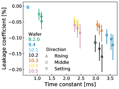
Figure 8: Coefficients of the leakage from the intensity $(0,0,\mathrm{Re})$ component to the circular polarization $(2,2,\mathrm{Im})$ component, plotted against the detector time constant. The color and shape of marks denote the wafer and scan direction, respectively. The points show median values and error bars show the observation-by-observation variation.

Figure 8 shows the estimated coefficients of leakage to the circular polarization $(2,2,\mathrm{Im})$ component. There is an appreciable dependence on the wafer in that the coefficient is almost zero for wafer 10.1 and approximately $-0.1$% for the other wafers. Wafer 10.1 has the largest saturation power and the shortest time constant, and thus the smallest nonlinearity. For the other wafers, the effects of time constant nonlinearity are observed, with the impact increasing in the slower wafers. In addition, the detector nonlinearity depends on the optical loading (i.e., the observing elevation and the weather conditions), which causes the variation in the leakage.

After subtraction of this leakage, the variation in the slope $p_{1,\mathrm{obs}}^{(2,2,\mathrm{Im})}$ decreases in all wafers except wafer 10.1. In particular, the standard deviation decreases by approximately 90% for wafer 10.2. Moreover, the coefficient of correlation between $p_{1,\mathrm{obs}}^{(0,0,\mathrm{Re})}$ and $p_{1,\mathrm{obs}}^{(2,2,\mathrm{Im})}$ decreases to $<7\%$ for all wafers. In addition, the coefficient of correlation between $p_{1,\mathrm{obs}}^{(2,2,\mathrm{Im})}$ and the leakage coefficient of this intensity subtraction is $<10\%$. Therefore, the systematic error due to the leakage of the intensity signal is well subtracted, and the residual should have a subdominant effect.

B.2 Polarization leakage

We next consider the leakage of the linear polarization signals, the $\tilde{d}^{(4,2,\mathrm{Re})}$ and $\tilde{d}^{(4,2,\mathrm{Im})}$ components. The source of these signals should be the instrumental polarization. The vertical polarization is created by the emission from the primary mirror in the off-axis optics (Takakura et al., 2017). The far sidelobe of the telescope may be polarized and create a polarized ground-synchronous signal. The contribution of the polarized ice clouds is mitigated by removing scans with polarized bursts during the data selection in Section 3.3.

As shown in Figure 3, we find a linear polarization signal with a non-zero azimuthal slope in both Stokes $Q$ and $U$. In particular, the rising observations in the fifth season have large slopes of several $\mathrm{mK}/\mathrm{rad}$. In this scan direction, we observe the lower sky close to the mountain on the east side of the telescope. Furthermore, the change in the fifth season might be due to the arrival of new containers for deployment of the Simons Array (see Figure 9).

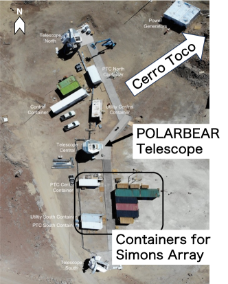
Figure 9: Aerial view of the Polarbear/Simons Array site. There are containers for the Simons Array to the south and southeast of the POLARBEAR telescope. A mountain, Cerro Toco, lies east of the telescope.

In the basic model with the nonidealities of the HWP (Section 2.4), the linear polarization signals $Q$ and $U$ leak into the imaginary part of the demodulated timestream of the second harmonic $\mathrm{Im}[\tilde{d}_{2}(t)]$ as $\rho(-Q\sin 2\phi+U\cos 2\phi)$. Owing to its dependency on the detector polarization angle $\phi$, this leakage should be accounted for separately in the detector averaging in Section 4.1, assuming the detector calibrations are accurate.

Another factor to consider is the effect of slant incidence on the HWP. In the Polarbear telescope, the HWP is placed at the prime focus, oriented so that its surface faces perpendicular to the main optical path. However, stray light creating the far sidelobe may arrive at a steep incident angle. In that case, the modulation of polarization signals is distorted, and there is thus leakage from the fourth harmonic to the second and sixth harmonics. This leakage is polarized and not separated by the detector averaging.

We estimate the coefficients of leakage from $(4,2,\mathrm{Re})$ and $(4,2,\mathrm{Im})$ components to the $(2,2,\mathrm{Im})$ component according to the correlation of the azimuthal slopes. We obtain the leakage coefficients $\lambda_{d}^{(4,2,\mathrm{Re})\rightarrow(2,2,\mathrm{Im})}$ and $\lambda_{d}^{(4,2,\mathrm{Im})\rightarrow(2,2,\mathrm{Im})}$ for each scan direction $d$ by minimizing:

$$\begin{split}&\sum_{\mathrm{obs}\in d}w_{\mathrm{obs}}\times\\ &\left(\Delta p_{1,\mathrm{obs}}^{(2,2,\mathrm{Im})}-\lambda_{d}^{(4,2,\mathrm{Re})\rightarrow(2,2,\mathrm{Im})}\Delta p_{1,\mathrm{obs}}^{(4,2,\mathrm{Re})}\right.\\ &\left.-\lambda_{d}^{(4,2,\mathrm{Im})\rightarrow(2,2,\mathrm{Im})}\Delta p_{1,\mathrm{obs}}^{(4,2,\mathrm{Im})}\right)^{2}\;.\end{split}$$ (B25)

Here, to prevent bias due to the atmospheric circular polarization signal’s dependence on the scan direction, we subtract the average for each scan direction $d$ as follows:

$$\Delta p_{1,\mathrm{obs}}^{(*)}=p_{1,\mathrm{obs}}^{(*)}-\frac{\sum_{\mathrm{obs}^{\prime}\in d}w_{\mathrm{obs}^{\prime}}\,p_{1,\mathrm{obs}^{\prime}}^{(*)}}{\sum_{\mathrm{obs}^{\prime}\in d}w_{\mathrm{obs}^{\prime}}}\;.$$ (B26)

These slopes have been adjusted for intensity leakage subtraction in all three components: $(4,2,\mathrm{Re})$, $(4,2,\mathrm{Im})$, and $(2,2,\mathrm{Im})$.

The statistical uncertainties in the leakage coefficients are estimated adopting the random sign-flip method, a type of bootstrap method. For each observation, we randomly assign a factor $f\in\{-1,1\}$ while ensuring that the weighted average remains zero. We then multiply $\Delta p_{1,\mathrm{obs}}^{(2,2,\mathrm{Im})}$ by this factor and perform the fitting for each realization. We repeat this process for many realizations and take the standard deviation of the results.

In addition, we estimate the systematic error from the potential seasonal variations of the leakage coefficients. In the above calculation, we use the same leakage coefficient for each wafer and scan direction assuming that it does not change over the seasons. In practice, however, the leakage coefficient may have seasonal variations. We estimate the leakage coefficients $\lambda_{d,y}^{(4,2,\mathrm{Re})\rightarrow(2,2,\mathrm{Im})}$ and $\lambda_{d,y}^{(4,2,\mathrm{Im})\rightarrow(2,2,\mathrm{Im})}$ using the subset of data for each season $y$. We then estimate the systematic uncertainty for each component such that the reduced chi-squared of the difference from the leakage coefficient becomes unity. This is expressed by:

$$\sum_{y\in\{3,4,5\}}\frac{\left(\lambda_{d,y}^{(4,2,\mathrm{Re})\rightarrow(2,2,\mathrm{Im})}-\lambda_{d}^{(4,2,\mathrm{Re})\rightarrow(2,2,\mathrm{Im})}\right)^{2}}{\left(\delta\lambda_{d,y,\mathrm{stat}}^{(4,2,\mathrm{Re})\rightarrow(2,2,\mathrm{Im})}\right)^{2}+\left(\delta\lambda_{d,\mathrm{sys}}^{(4,2,\mathrm{Re})\rightarrow(2,2,\mathrm{Im})}\right)^{2}}=1\;.$$ (B27)

Finally, the total uncertainty of $\lambda_{d}^{(4,2,\mathrm{Re})\rightarrow(2,2,\mathrm{Im})}$ is estimated as:

$$\begin{split}\left(\delta\lambda_{d,\mathrm{tot}}^{(4,2,\mathrm{Re})\rightarrow(2,2,\mathrm{Im})}\right)^{2}=&\left(\delta\lambda_{d,\mathrm{stat}}^{(4,2,\mathrm{Re})\rightarrow(2,2,\mathrm{Im})}\right)^{2}\\ &+\left(\delta\lambda_{d,\mathrm{sys}}^{(4,2,\mathrm{Re})\rightarrow(2,2,\mathrm{Im})}\right)^{2}\;.\end{split}$$ (B28)

We perform the same calculation for the $(4,2,\mathrm{Im})$ component.

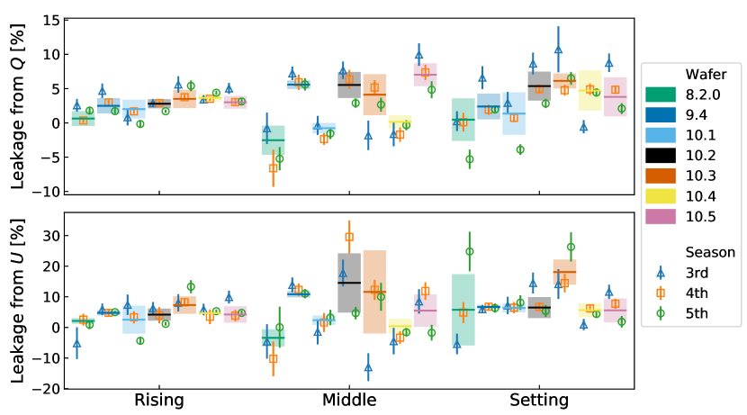
Figure 10: Estimated coefficients of the leakage from the linear polarization components $(4,2,\mathrm{Re})$ and $(4,2,\mathrm{Im})$ (corresponding to Stokes $Q$ and $U$) into the circular polarization signal $(2,2,\mathrm{Im})$. Each panel shows the leakage for each wafer and polarization. Each point shows the leakage value and statistical uncertainty for each scan direction and season. A black line shows the value obtained from all data for each scan direction, and a box shows its uncertainty including both the statistical and systematic uncertainties.

Figure 10 shows the estimated leakage coefficients and their uncertainties. The amplitudes of the leakage coefficients are $\lesssim 10\%$.

We subtract the leakage for each observation according to:

$$\begin{split}p_{1,\mathrm{obs}}^{\prime(2,2,\mathrm{Im})}=&p_{1,\mathrm{obs}}^{(2,2,\mathrm{Im})}-\lambda_{d}^{(4,2,\mathrm{Re})\rightarrow(2,2,\mathrm{Im})}p_{1,\mathrm{obs}}^{(4,2,\mathrm{Re})}\\ &-\lambda_{d}^{(4,2,\mathrm{Im})\rightarrow(2,2,\mathrm{Im})}p_{1,\mathrm{obs}}^{(4,2,\mathrm{Im})}\;.\end{split}$$ (B29)

This leakage subtraction decreases the standard deviation of slope $p_{1,\mathrm{obs}}^{(2,2,\mathrm{Im})}$ by approximately $10\%$ for wafer 8.2.0 and $80\%$ for wafer 10.4.

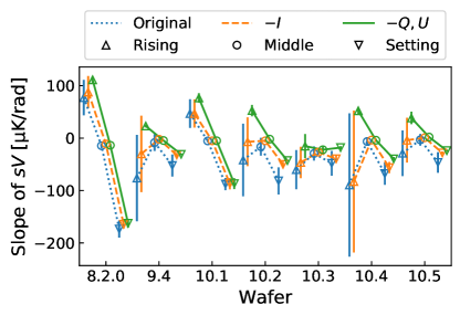
Figure 11: Effect of the intensity and linear polarization subtraction in the circular polarization measurement. The points show the slope of the circular polarization signals for each wafer and scan direction at different stages of leakage subtraction. The blue points are values without leakage subtraction. The orange points are values after subtracting leakage from the intensity signal. The green points are final values after accounting for leakage from both the intensity and linear polarization.

Figure 11 shows the effect of the leakage subtractions. We find that both intensity and linear polarization subtractions, especially linear polarization subtraction, affect the results of the azimuthal slope.

References

- Abazajian et al. (2016) Abazajian, K. N., Adshead, P., Ahmed, Z., et al. 2016, arXiv preprint arXiv:1610.02743, doi: 10.48550/arXiv.1610.02743
- Ade et al. (2019) Ade, P., Aguirre, J., Ahmed, Z., et al. 2019, Journal of Cosmology and Astroparticle Physics, 2019, 056, doi: 10.1088/1475-7516/2019/02/056
- Aghanim et al. (2020) Aghanim, N., Akrami, Y., Ashdown, M., et al. 2020, Astronomy & Astrophysics, 641, A6, doi: 10.1051/0004-6361/201833910
- Arnold et al. (2012) Arnold, K., Ade, P. A., Anthony, A., et al. 2012, in Millimeter, Submillimeter, and Far-Infrared Detectors and Instrumentation for Astronomy VI, Vol. 8452, SPIE, 381–392, doi: 10.1117/12.927057
- Brown et al. (2004) Brown, R. L., Wild, W., & Cunningham, C. 2004, Advances in Space Research, 34, 555, doi: 10.1016/j.asr.2003.03.028
- Caloni et al. (2023) Caloni, L., Giardiello, S., Lembo, M., et al. 2023, Journal of Cosmology and Astroparticle Physics, 2023, 018, doi: 10.1088/1475-7516/2023/03/018
- Chulliat (2015) Chulliat, A. 2015, The Enhanced Magnetic Model 2015-2020, National Centers for Environmental Information, NOAA, doi: 10.7289/V56971HV
- Coerver et al. (2024) Coerver, A., Zebrowski, J., Takakura, S., et al. 2024, arXiv preprint arXiv:2407.20579, doi: 10.48550/arXiv.2407.20579
- Cooray et al. (2003) Cooray, A., Melchiorri, A., & Silk, J. 2003, Physics Letters B, 554, 1, doi: 10.1016/S0370-2693(02)03291-4
- De & Tashiro (2015) De, S., & Tashiro, H. 2015, Physical Review D, 92, 123506, doi: 10.1103/PhysRevD.92.123506
- Errard et al. (2015) Errard, J., Ade, P., Akiba, Y., et al. 2015, The Astrophysical Journal, 809, 63, doi: 10.1088/0004-637X/809/1/63
- Essinger-Hileman (2013) Essinger-Hileman, T. 2013, Applied optics, 52, 212, doi: 10.1364/AO.52.000212
- Finelli & Galaverni (2009) Finelli, F., & Galaverni, M. 2009, Physical Review D, 79, 063002, doi: 10.1103/PhysRevD.79.063002
- Fujino et al. (2023) Fujino, T., Takakura, S., Chinone, Y., et al. 2023, Review of Scientific Instruments, 94, 064502, doi: 10.1063/5.0140088
- Hanany & Rosenkranz (2003) Hanany, S., & Rosenkranz, P. 2003, New A Rev., 47, 1159, doi: 10.1016/j.newar.2003.09.017
- Hill et al. (2016) Hill, C. A., Beckman, S., Chinone, Y., et al. 2016, in Millimeter, Submillimeter, and Far-Infrared Detectors and Instrumentation for Astronomy VIII, Vol. 9914, SPIE, 699–716, doi: 10.1117/12.2232280
- Hoseinpour et al. (2020) Hoseinpour, A., Zarei, M., Orlando, G., Bartolo, N., & Matarrese, S. 2020, Physical Review D, 102, 063501, doi: 10.1103/PhysRevD.102.063501
- Keating et al. (1998) Keating, B., Timbie, P., Polnarev, A., & Steinberger, J. 1998, ApJ, 495, 580, doi: 10.1086/305312
- Kermish et al. (2012) Kermish, Z. D., Ade, P., Anthony, A., et al. 2012, in Millimeter, Submillimeter, and Far-Infrared Detectors and Instrumentation for Astronomy VI, Vol. 8452, SPIE, 366–380, doi: 10.1117/12.926354
- Lenoir (1968) Lenoir, W. B. 1968, Journal of Geophysical Research, 73, 361, doi: 10.1029/JA073i001p00361
- Li et al. (2023) Li, Y., Appel, J. W., Bennett, C. L., et al. 2023, The Astrophysical Journal, 958, 154, doi: 10.3847/1538-4357/ad0233
- LiteBIRD Collaboration (2023) LiteBIRD Collaboration. 2023, Progress of Theoretical and Experimental Physics, 2023, 042F01, doi: 10.1093/ptep/ptac150
- Matsuda et al. (2019) Matsuda, F., Lowry, L., Suzuki, A., et al. 2019, Review of Scientific Instruments, 90, 115115, doi: 10.1063/1.5095160
- Meeks & Lilley (1963) Meeks, M. L., & Lilley, A. E. 1963, Journal of Geophysical Research, 68, 1683, doi: 10.1029/JZ068i006p01683
- Mohammadi (2014) Mohammadi, R. 2014, The European Physical Journal C, 74, 1, doi: 10.1140/epjc/s10052-014-3102-1
- Nagy et al. (2017) Nagy, J., Ade, P., Amiri, M., et al. 2017, The Astrophysical Journal, 844, 151, doi: 10.3847/1538-4357/aa7cfd
- Navas-Guzmán et al. (2015) Navas-Guzmán, F., Kämpfer, N., Murk, A., et al. 2015, Atmospheric Measurement Techniques, 8, 1863, doi: 10.5194/amt-8-1863-2015
- Paine (2022) Paine, S. 2022, The am atmospheric model, 12.2, Zenodo, doi: 10.5281/zenodo.6774376
- Petroff et al. (2020) Petroff, M. A., Eimer, J. R., Harrington, K., et al. 2020, ApJ, 889, 120, doi: 10.3847/1538-4357/ab64e2
- Polarbear Collaboration (2020) Polarbear Collaboration. 2020, ApJ, 897, 55, doi: 10.3847/1538-4357/ab8f24
- Polarbear Collaboration (2022) —. 2022, ApJ, 931, 101, doi: 10.3847/1538-4357/ac6809
- Spinelli et al. (2011) Spinelli, S., Fabbian, G., Tartari, A., Zannoni, M., & Gervasi, M. 2011, MNRAS, 414, 3272, doi: 10.1111/j.1365-2966.2011.18625.x
- Sugiyama et al. (2024) Sugiyama, J., Terasaki, T., Sakaguri, K., et al. 2024, Journal of Low Temperature Physics, 214, 173, doi: 10.1007/s10909-023-03036-3
- Takakura et al. (2017) Takakura, S., Aguilar, M., Akiba, Y., et al. 2017, J. Cosmology Astropart. Phys, 2017, 008, doi: 10.1088/1475-7516/2017/05/008
- Takakura et al. (2019) Takakura, S., Aguilar-Faúndez, M. A. O., Akiba, Y., et al. 2019, ApJ, 870, 102, doi: 10.3847/1538-4357/aaf381
- Thompson et al. (1980) Thompson, A. R., Clark, B., Wade, C., & Napier, P. J. 1980, Astrophysical Journal Supplement Series, vol. 44, Oct. 1980, p. 151-167., 44, 151, doi: 10.1086/190688