Music102: An -equivariant transformer for chord progression accompaniment
1 Introduction
In the burgeoning age of AI arts, generative AI represented by the diffusion model has been profoundly influencing the concept of digital paintings, while music production remains a frontier for machine intelligence to explore. For an AI composer, there’s a long way to achieve the holy grail of creating a complete classical symphony, however, simpler tasks such as fragment generation and accompaniment are within our reach. Inspired by the wide demand from music education and daily music practice, we designed a prototypical model, Music101, which succeeded in predicting a reasonable chord progression given the single-track melody of pop music. Although the model was observed to have captured some essential music patterns, its performance was still far from a real application. The quantity and the quality of the available dataset are quite limited, so any complication of the architecture didn’t benefit the previous experiments.
Nevertheless, there are hidden inductive biases in this task to be leveraged. Between music and mathematics is a natural connection, especially in the language of symbolic music. With equal temperament, transposition, and reflection symmetry emerge from the pitch classes on the keyboard. The conscious application of group theory on music dates back to Schoenberg’s atonality music, and the relevant group actions have long been in the toolbox of classical composers even earlier than Bach. In this work, we proposed Music102, encodes prior knowledge of music by leveraging this symmetry in the music representation.
2 Related work
The notion of the symmetry of pitch classes is fundamental in music theory Mazzola (2012), where the group theory exerts its power as in spatial objects Papadopoulos (2014). As an essential prior knowledge of the music structure, computational music studies have embraced it in various tasks, such as transposition-invariant music metric Hadjeres and Nielsen (2017), transposition-equivariant pitch estimation Riou et al. (2023); Cwitkowitz and Duan (2024). Some work tried to extract this structure from music pieces in priori as well Lostanlen et al. (2020).
Between notes and words, there is an analogy between natural languages and music. Therefore, popular frameworks for natural language tasks, especially the transformer, are proven indispensable in symbolic music understanding and generation with the awareness of inherent characteristics of music, like the long-term dependence and timescale separation explored in Music transformer Huang et al. (2019) and Museformer Yu et al. (2022). The triumphs in the time domain encourage us to focus on the rich structures in the frequency domain, that is the pitch classes in symbolic music.
The introduction of equivariance into attentive layers has been paid much attention in building expressive and flexible models for grid, sequence, and graph targets. SE(3)-transformer Fuchs et al. (2020) provides a good example of how the attention mechanism works naturally with invariant attention scores and equivariant value tensors. The non-linearity and layer normalization layer in this work is inspired by Equiformer Liao and Smidt (2022); Liao et al. (2023) and the implementation of activation in E3NN Geiger and Smidt (2022).
3 Background
3.1 Equal temperament
The notion of a sound’s pitch is physically instantiated by the frequency of its vibration. Due to the physiological features of human ears and/or centuries of cultural construction, sounds of frequencies with a simple integer ratio make people feel harmonious. The relation between two pitches with the simplest non-trivial ratio, , is called an octave, the best harmony we can create. Based on the octave, pitches with a frequency ratio of build an equivalence relation, which partitions the set of pitches into pitch classes.
However, all frequencies are not implemented in music instruments neither allowed in most music compositions. A temperament is a criterion for how people define the relationship between legal pitches among available frequencies. One of the most essential topics of the temperament is how to make it finer-grained to accommodate useful pitches. The equal temperament is the most popular scheme in modern music. It subdivides an octave into 12 minimal intervals, called semitones or keys, each of which is a multiple of on the frequency. Their equality is manifested on the logarithm scale of the frequency. Starting from a pitch class , a set of 12 pitch classes spanning the octave is iteratively defined by the semitone. Each of their pitch class name as a letter and its ordinal number in the frequency ascending order are in Table 1. Some pitch classes have two equivalent names in the equal temperament, with preference only when discussing the interaction between pitch classes.
| 0 | 1 | 2 | 3 | 4 | 5 | 6 | 7 | 8 | 9 | 10 | 11 |
A pitch in the pitch class has a pitch name , where the subscript , called octave number, distinguishes frequencies in the same class . The difference in octave numbers relates to the frequency ratio in octaves between the pitches as
| (1) |
then a pitch class is composed of . Within the same octave number , pitches are connected by the distance in their ordinal numbers as
| (2) |
According to this notation, any frequency corresponding to a pitch name can be determined by the reference frequency of one pitch. is the most popular standard in the music community.
is isomorphic to by a vectorization function defined on any of its elements as . The collection of these vectors is a basis of .
The piano is an instrument that usually follows an equal temperament. Its keyboard is grouped by the octave number. Each group contains the keys corresponding to the pitches to with the same octave number, illustrated in Figure 1.
3.2 Symbolic music
A piece of music is a time series. The simplest practice of composing music is picking pitches and deciding the key time points when they sound and mute. These key time points usually follow some pattern called the rhythm. The rhythm allows for the recognition of the beat as a basic unit of the musical time. A series of beats sets an integer grid on the time axis. A sound usually starts at some simple rational point in this grid, and its timespan called the value, is also some simple fraction of one beat.
Thus, the temperament sets a coordinate system in the frequency domain, and the beat series sets a coordinate system in the time domain. On these coordinate systems, a segment with a pitch on the frequency axis, a starting beat and a value along the time axis, is called a note , the information unit of music. A symbolic system, such as the music score, can record a piece of music with the symbol of the coordinate systems and the notes on it, which is the foundation of symbolic music. Once a reference frequency of one pitch is chosen, like , the frequency of each pitch is determined. Once the length of the beats in the wall time, or the tempo, is chosen, the key time point of each sound is determined. More information for the music performance, such as timbres (spectrum signatures that feature an instrument), articulations (playing techniques), and dynamics (local treatments on the speed and the volume), can be also annotated in the symbolic music. With these parameters, players with instruments or synthesizers lift the symbolic music to the playing audio.
3.3 Chord
The combination of multiple pitches forms a chord. By virtue of the octave equivalence, a chord can be simplified as a combination of pitch classes, namely . Then with the ordinal number , every chord is naturally expressed as a set of number , or a binary vector where the entry is the value of an indicator function . Another equivalent expression is
The theory of harmony studies the interaction between pitches under a temperament. It reveals that different combinations have different musical colors and functions. For example, a C major chord, , is bright and stable, while a C minor chord, , is dim and tense.
3.3.1 Transposition
We define the transposition operator . When it acts on a pitch,
When it acts on a pitch class,
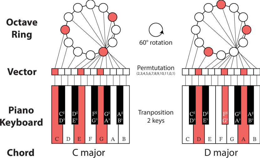
In Figure 1, we apply , a transposition of two semitones, to the C major chord , arriving at the chord , which is called the D major chord in harmony theory. Harmony theory points out that a transposition doesn’t change the color of a chord, but shifts the tone of a chord. Thus the transposed chord always hears similar to the original one but adapts to another set of pitches.
It’s easy to verify
thus for the action on
This means that , linking the tail of an octave with the head. As shown at the top of Figure 1, each pitch class can be mapped into an octave ring, where forms a dodecagon inscribed in the circle, and corresponds to the rotation by , which leaves the dodecagon invariant. By checking the definition, forms a group,
This geometric intuition indicates that it is isomorphic to the cyclic group or the rotation group . A transposition operator on is equivalent to a group action of on .
When it acts on a chord, we define
Thanks to the isomorphism , there exists a group homomorphism that satisfies
and it’s obvious that every is a permutation matrix. is a permutation representation of .
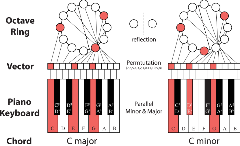
3.3.2 Reflection
We define the reflection operator . In a pitch class, it acts as
and on a chord, it acts as
The behavior of on the octave circle is a reflection w.r.t. the mirror passing through the vertex and the vertex of the inscribed dodecagon. It is more general to think of the semidirect product . Each transformation in the product with the form is a reflection with a mirror either passing through two opposite vertices or passing through the middle points of two opposite edges of the inscribed dodecagon, leaving the dodecagon invariant. This geometry adopts dihedral group or the isomorphic . The transposition-reflection on is equivalent to a group action of on .
Because is a subgroup of , the previous representation of induces , which satisfies
In Figure 2, we get . The underlying mirror is the dashed line. Harmony theory says that a reflection changes the color of a chord, switching between the bright, stable major chords and dim, tense minor chords, but if composed with an appropriate transposition, it keeps the tone.
3.4 Homophony
Homophony is a music composition framework, in which a music has a primary part called the melody and other auxiliary parts called the accompaniment. Most pop music follows it with a vocal melody and instrumental accompaniments. One of the most important accompaniment formats is the chord progression, a time series of chords with their starting beats and values with no timespan overlap. It can be further detailed as a note series for performance by some texture, but the chord itself has included pivotal information to fulfill the musical requirement of the whole piece. The relationship of the melody notes and the chord progression is restricted by the harmony theory as a probability distribution like a generative model. For a simpler predictive model, it learns the map from the melody to the best chord progression .
The transformation defined above should apply to the whole piece of music. Transposition on the melody is the overall key shift, and its combination with reflection is involved in the major-minor variation. As a result, the harmony restriction requires that the accompaniment, especially the chord progression, should transform accordingly. For a generative model, this implies a equivariant distribution . For a predictive model, it needs to learn an equivariant function where holds.
4 Method
4.1 Embedding music into vectors
A minimum value of is used as a time step. The melody notes are embedded as a series of vectors , where records the sounding notes during the timespan between and . Inspired by Lin and Yeh (2017), the embedding builds on the relative contribution of each note during the timespan.
The chord progression can be similarly embedded as vectors , however, the chord progression is much sparser than the melody notes. If is small enough (e.g. half beat), will be the common factor of every and , thus the term will be binary. And because of no timespan overlap in the chord progression, each summation has exactly one term. In this case, itself is the vectorized form of one chord, that is the chord state during the time between and . The collection of describes a state transition series.
This featurization naturally pulls the group action on pitch classes back to the permutation representation on . If there are totally time steps, we collect the melody vectors of as a matrix and the chord vectors of as a matrix , then the featurization of is for all .
We aim to build a predictive model which takes in and predicts . Hence, its equivariant condition is
| (3) |
4.2 Decomposition of the permutation representation
is a 12-dimensional reducible representation. According to the character table (Table 2), it can be canonically decomposed into
| (4) |
which means the components transformed as or vanish. Because the non-zero coefficients in the canonical decomposition (Equation 4) are all one, the solution of change of basis matrix via
| (5) |
is unique up to an isomorphism. For the sake of a simple and stable neural network training, we have to be
-
•
Real: This possibility is guaranteed because all the irreducible representations of are real inherently.
-
•
Orthogonal: . This can be realized by normalizing the solution.
Then each has its pre-determined value stored as a constant before invoking the neural network.
4.3 An overview of the Music10x model
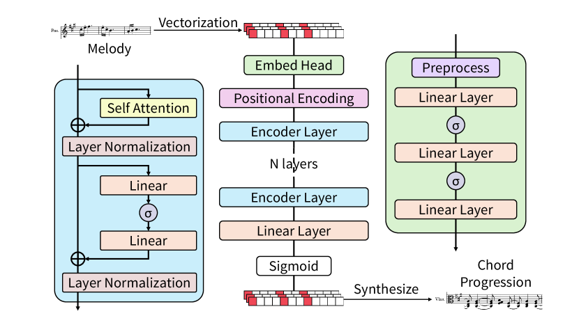
As illustrated in Figure 3, Music101 and Music102 share the same backbone. The preprocessing layer in Music101 is an identity map, and the other layers follow the traditional implementation in a transformer Vaswani et al. (2017). As a result, Music101 doesn’t naturally satisfy the equivariant condition Equation 3.
In Music102, the linear layer, the positional encoding, the self-attention layer, the layer normalization, and the non-linearity are reformulated to be equivariant, as detailed in the following section.
4.4 -equivariant layers
-preprocessing
For each column vector in which transforms as , a -featurization layer pushes it forward to a representation vector belongs to -channel by
where is a learnable scalar and is a vector of ones. We can check that
thus from the -featurization layer transforms as .
-equivariant linear layers
composed of column vectors in -channel is a matrix in -channel with multiplicity . According to the Schur’s lemma, is the only weight in the linear layer that keeps the equivariance between two channels. Therefore, the general linear layer is only within the same channel, parametrized as a learnable weight that maps to .
-equivariant activation function
Common activation functions, like ReLU or Sigmoid, don’t behave equivariantly between linear layers. However, if a vector transforms as a that maps the -th element to -th one, for any element-wise function , we have
| (6) |
that is, any element-wise function commutes with the permutation representation, including any common non-linearity we may apply.
Take the transposition of the Equation 5, it holds for any that
It is possible to have both and orthogonal representations, which leads to
for any . Thus is the matrix that pulls the -channel vector back to the permutation representation. Then a non-linearity can be incorporated by in -channel, because
-equivariant positional encoding
The positional encoding is added to the sequential features to make the self-attention mechanism position-aware. For a sequence of -dimensional word embedding , the encoded sequence is
In our -equivariant architecture, the sequence in -channel with multiplicity is a tensor , where is a matrix in -channel. We define the positional encoding for -channel as
Because is a constant along the representation dimension, the permutation acts trivially . It follows that
thus the positional encoding is equivariant.
-equivariant multihead self-attention
Through -equivariant linear layers, the sequence is transformed into the query sequence , the key sequence , and the value sequence in each channel. We split the multiplicity of sequences , into heads and concatenate different channels as
. Obviously the concatenated sequence transforms as the representation , which is orthogonal when all the is orthogonal. When this concatenation applies to and results in , the attention weight becomes invariant by virtue of the orthogonality of because
The weighted sum naturally transforms as a representation which follows.
This mechanism also applies to multi-head attention if each head’s queries and keys follow the same orthogonal representation.
-equivariant layer normalization
Taking advantage of the Equation 6 and that the permutation doesn’t affect vector elements’ variance and mean, we define the layer normalization as
where takes the variance of all elements of the input, takes the mean, is a small positive number for numerical stability, and are learnable parameters.
4.5 Loss function
A weighted binary cross-entropy loss is defined between the predicted , whose each column is the logit of the 12 pitches, and the ground truth .
The weights emphasize the chord transition point by
5 Experiments
The code conducting the experiments can be found in our Github repo.
5.1 Data Acquisition and processing
The model is trained on POP909 Dataset Wang et al. (2020), which contains 909 pieces of Chinese pop music with the melody stored in MIDI and the chord progression annotation stored as time series. We extract the melody from the MIDI file of each song and match it with the chord progressions and beat annotations using the time stamps. The minimal is set to be 1/2 beat in our experiments. The dataset is randomly split into 707 pieces in the training set, 100 pieces in the validation set, and 100 pieces in the test set. The vectorization and the loss weights are precomputed before training.
5.2 Comments on the numerical stability
We tried another flavor of equivariant non-linearities and layer normalizations adopted in Equiformer Liao and Smidt (2022) and SE(3)-transformer Fuchs et al. (2020), the norm-gated ones. For instance, the non-linearity acting on an equivariant vector can remain equivariant by the invariance of the norm under unitary representations.
However, due to the sparsity of the input melody (a large number of zero column vectors in ), the norm at the denominator induces unavoidable gradient explosion, which usually halts the training after several batches or epochs even combined with a small constant bias or trainable equivariant biases. This is one of the motivations during the experiment of shifting the non-linearity, the positional encoding, and the layer normalization to a vector transforming as the permutation representation by Equation 6. It is the key observation that enables the whole experiment after dozens of modified versions of the norm-gated flavor.
5.3 Music synthesis and auditory examples
The output is rounded as a binary with a cutoff of logit 0.5. Mapping back to the pitch classes, MuseScore4 synthesizes the input melody and the output chord progression simultaneously to be a piece of complete music. (Link to audio examples from Music102 output on the test set, as well as transposed versions of one piece to demonstrate its equivariance).
5.4 Comparison between Music101 and Music102
Limited by the computation resource and time, the hyperparameters haven’t been thoroughly scanned but locally searched on several key components, including the length of features, the number of encoding layers, and the learning rate, arriving at a suboptimal amount of parameters.
In addition to the loss itself, the other two metrics also evaluate the performance of the model reproducing the chord progression label. The cosine similarity is defined as
The exact accuracy is defined as
As shown in Table 3( means the lower the better, means the higher the better). Music102 reaches a better performance with less amount of parameters.
| Model (Amount of Params) | Music102 (760030) | Music101 (6850060) |
|---|---|---|
| Weighted BCE loss () | 0.5652 | 0.5807 |
| Cosine similarity () | 0.6727 | 0.6638 |
| Exact accuracy () | 0.1783 | 0.1141 |
6 Conclusion
To the best of our knowledge, this is the first transformer-based seq2seq model that considers the word-wise symmetry in the input and output word embeddings. As a result, the universal schemes in the transformer for natural language processing, including layer normalization and positional encoding, need to be adapted to this new domain. Our modification from a traditional transformer Music101 to the fully equivariant Music102 without essential backbone change shows that there are out-of-the-box equivariant substitutions of a self-attention-based sequence model. Taking full advantage of the property of the permutation representation, we explore a more flexible and stable framework of equivariant neural networks on a discrete group.
Given the efficiency and accuracy of the chord progression task, we expect that Music102 could be a general backbone of the equivariant music generation model in the future. We believe that the mathematical structure within the music provides further implications for computational music composing and analysis.
Acknowledgement
The author thanks Yucheng Shang (ycshang@mit.edu) and Weize Yuan (w96yuan@mit.edu) for their previous endeavor for Music101 prototype.
References
- Cwitkowitz and Duan [2024] Frank Cwitkowitz and Zhiyao Duan. Toward fully self-supervised multi-pitch estimation. arXiv preprint arXiv:2402.15569, 2024.
- Fuchs et al. [2020] Fabian Fuchs, Daniel Worrall, Volker Fischer, and Max Welling. Se (3)-transformers: 3d roto-translation equivariant attention networks. Advances in neural information processing systems, 33:1970–1981, 2020.
- Geiger and Smidt [2022] Mario Geiger and Tess Smidt. e3nn: Euclidean neural networks. arXiv preprint arXiv:2207.09453, 2022.
- Hadjeres and Nielsen [2017] Gaëtan Hadjeres and Frank Nielsen. Deep rank-based transposition-invariant distances on musical sequences. arXiv preprint arXiv:1709.00740, 2017.
- Huang et al. [2019] Cheng-Zhi Anna Huang, Ashish Vaswani, Jakob Uszkoreit, Ian Simon, Curtis Hawthorne, Noam Shazeer, Andrew M. Dai, Matthew D. Hoffman, Monica Dinculescu, and Douglas Eck. Music transformer. In International Conference on Learning Representations, 2019. URL https://openreview.net/forum?id=rJe4ShAcF7.
- Liao and Smidt [2022] Yi-Lun Liao and Tess Smidt. Equiformer: Equivariant graph attention transformer for 3d atomistic graphs. arXiv preprint arXiv:2206.11990, 2022.
- Liao et al. [2023] Yi-Lun Liao, Brandon Wood, Abhishek Das, and Tess Smidt. Equiformerv2: Improved equivariant transformer for scaling to higher-degree representations. arXiv preprint arXiv:2306.12059, 2023.
- Lin and Yeh [2017] Bor-Shen Lin and Ting-Chun Yeh. Automatic chord arrangement with key detection for monophonic music. In 2017 International Conference on Soft Computing, Intelligent System and Information Technology (ICSIIT), pages 21–25. IEEE, 2017.
- Lostanlen et al. [2020] Vincent Lostanlen, Sripathi Sridhar, Brian McFee, Andrew Farnsworth, and Juan Pablo Bello. Learning the helix topology of musical pitch. In ICASSP 2020-2020 IEEE International Conference on Acoustics, Speech and Signal Processing (ICASSP), pages 11–15. IEEE, 2020.
- Mazzola [2012] Guerino Mazzola. The topos of music: geometric logic of concepts, theory, and performance. Birkhäuser, 2012.
- Papadopoulos [2014] Athanase Papadopoulos. Mathematics and group theory in music. arXiv preprint arXiv:1407.5757, 2014.
- Riou et al. [2023] Alain Riou, Stefan Lattner, Gaëtan Hadjeres, and Geoffroy Peeters. Pesto: Pitch estimation with self-supervised transposition-equivariant objective. In International Society for Music Information Retrieval Conference (ISMIR 2023), 2023.
- Vaswani et al. [2017] Ashish Vaswani, Noam Shazeer, Niki Parmar, Jakob Uszkoreit, Llion Jones, Aidan N Gomez, Ł ukasz Kaiser, and Illia Polosukhin. Attention is all you need. In I. Guyon, U. Von Luxburg, S. Bengio, H. Wallach, R. Fergus, S. Vishwanathan, and R. Garnett, editors, Advances in Neural Information Processing Systems, volume 30. Curran Associates, Inc., 2017. URL https://proceedings.neurips.cc/paper_files/paper/2017/file/3f5ee243547dee91fbd053c1c4a845aa-Paper.pdf.
- Wang et al. [2020] Ziyu Wang, K. Chen, Junyan Jiang, Yiyi Zhang, Maoran Xu, Shuqi Dai, Xianbin Gu, and Gus G. Xia. Pop909: A pop-song dataset for music arrangement generation. In International Society for Music Information Retrieval Conference, 2020. URL https://api.semanticscholar.org/CorpusID:221140193.
- Yu et al. [2022] Botao Yu, Peiling Lu, Rui Wang, Wei Hu, Xu Tan, Wei Ye, Shikun Zhang, Tao Qin, and Tie-Yan Liu. Museformer: Transformer with fine- and coarse-grained attention for music generation. In Alice H. Oh, Alekh Agarwal, Danielle Belgrave, and Kyunghyun Cho, editors, Advances in Neural Information Processing Systems, 2022. URL https://openreview.net/forum?id=GFiqdZOm-Ei.