Deep Autoencoder with SVD-Like Convergence and Flat Minima

Abstract

Representation learning for high-dimensional, complex physical systems aims to identify a low-dimensional intrinsic latent space, which is crucial for reduced-order modeling and modal analysis. To overcome the well-known Kolmogorov barrier, deep autoencoders (AEs) have been introduced in recent years, but they often suffer from poor convergence behavior as the rank of the latent space increases. To address this issue, we propose the learnable weighted hybrid autoencoder, a hybrid approach that combines the strengths of singular value decomposition (SVD) with deep autoencoders through a learnable weighted framework. We find that the introduction of learnable weighting parameters is essential — without them, the resulting model would either collapse into a standard POD or fail to exhibit the desired convergence behavior. Additionally, we empirically find that our trained model has a sharpness thousands of times smaller compared to other models. Our experiments on classical chaotic PDE systems, including the 1D Kuramoto-Sivashinsky and forced isotropic turbulence datasets, demonstrate that our approach significantly improves generalization performance compared to several competing methods, paving the way for robust representation learning of high-dimensional, complex physical systems.

[1]organization=Department of Mechanical, Aerospace, and Nuclear Engineering, Rensselaer Polytechnic Institute, addressline=110 8th St, city=Troy, postcode=12180, state=New York, country=USA

[2]organization=Scientific Computation Research Center, Rensselaer Polytechnic Institute, addressline=110 8th St, city=Troy, postcode=12180, state=New York, country=USA

We propose a novel learnable weighted hybrid autoencoder for dimensionality reduction of complex physical systems.

The proposed deep autoencoder shows SVD-like convergence.

Learnable weighting parameters play a key role in achieving the enhanced performance.

The minima of our framework exhibit orders of magnitude smaller sharpness than other deep autoencoders, which leads improved noise robustness and generalization.

1 Introduction

Computational fluid dynamics involves solving large dynamical systems with millions of degrees of freedom, resulting in significant computational overhead. In order to alleviate this problem, reduced order modeling [1] is widely employed, which uses a smaller number of modes to provide approximate solution at lower computational expense. A crucial step in reduced-order modeling is the projection of system states to a reduced latent space. The projection error onto the latent space represents the overhead error that affects the solution accuracy throughout the time-stepping scheme. Linear dimensionality reduction techniques such as Proper Orthogonal Decomposition (POD) [2, 3, 4] are often used to create efficient representations of large-scale systems by projecting the solution manifold onto the space spanned by a set of linear orthonormal basis. Advances in deep learning techniques, such as deep autoencoders (AE) [5], capture intrinsic nonlinear features for better compression and retrieval of high-fidelity information, outperforming POD at lower ranks, thus overcoming the well-known Kolmogorov barrier [6, 7]. Milano and Koumoutsakos [8] highlighted one of the earliest works of utilizing a fully-connected autoencoder in reconstructing the flow field, offering better performance as compared to POD. Further studies have reported the usage of convolutional neural networks on 2D or 3D flow fields [9, 10, 11]. Such methods have been adopted in the fluid dynamics community to obtain a non-linear model order reduction [12], but they do not provide rapid error convergence at higher rank. Recently, there have also been studies on using hybrid approach [13, 14] combining POD with deep learning, by passing the latent space produced by POD to a neural network to find the corrections required to enhance the reconstruction. These hybrid techniques have proven to enhance the reconstruction beyond the capabilities of vanilla autoencoders. Following a similar path, here we propose a novel dimensionality reduction technique that combines traditional dimensionality reduction technique, i.e., POD, with deep learning techniques in a weighted manner at the encoder and decoder stage, where such weights of hybridization are also learnt from data, to achieve a more effective and flexible dimensionality reduction. We also compare this approach with a straightforward hybrid technique, where a direct sum of POD and AE is utilized to construct the autoencoder, demonstrating the need of using learnable weighting parameters between POD and AE. Interestingly, our proposed approach obtains a flat minima as opposed to other approaches, which contributes to the improved generalization and noise robustness.

2 Methodology

Without loss of generality, we begin with sampling a general vector-valued spatial-temporal field $u(x,t)\in\mathbb{R}^{Q}$ on a fixed mesh with $N$ cells, where $(x,t)$ is the space-time coordinate. At each time $t$, a cell-centered snapshot sample is a matrix $\mathbf{x}\in\mathbb{R}^{N\times Q}$. In the current framework, we start with two encoders: 1) POD based encoder using $r$-dominant left singular vectors from the matrix consisting of stacked flattened columns of $\mathbf{x}$, denoted as $\phi_{\textrm{POD}}$. 2) the neural network encoder with output dimension as $r$, denoted as $\phi_{\textrm{NN}}$. As shown in eq. 1, the latent state $\mathbf{z}\in\mathbb{R}^{r}$ is obtained by a weighted sum of POD projection and the output of encoder,

$$\mathbf{z}=(\mathbf{1}-\mathbf{a})\phi_{\textrm{POD}}(\mathbf{x})+\mathbf{a}\phi_{\textrm{NN}}(\mathbf{x}),$$ (1)

where $\mathbf{1}\in\mathbb{R}^{r}$ is a vector of ones, and $\mathbf{a}\in\mathbb{R}^{r}$ is a vector of learnable weights. Next for the decoder part, we project the latent state $\mathbf{z}$ back to the reconstructed system state following eq. 2,

$$\hat{\mathbf{x}}=\psi_{\textrm{POD}}(\mathbf{z})(\mathbf{I}-\mathbf{B})+\psi_{\textrm{NN}}(\mathbf{z})\mathbf{B},$$ (2)

where $\mathbf{I}$ is $Q\times Q$ identity matrix, $\mathbf{B}=\textrm{diag}(\mathbf{b})$, $\mathbf{b}\in\mathbb{R}^{Q}$, $\psi_{\textrm{POD}}$, and $\psi_{\textrm{NN}}$ are POD decoder and NN decoder, respectively. In addition to the parameters of NN encoder and decoder, both $\mathbf{a}\in\mathbb{R}^{r}$ and $\mathbf{b}\in\mathbb{R}^{Q}$ are trainable through gradient-based optimization as well. Hence, we name the above framework as learnable weighted hybrid autoencoder. It is important to note that such NN can be either fully-connected or convolutional.

Given the training dataset $\mathcal{D}=\{\mathbf{x}_{i}\}_{i=1}^{M}$, we trained the autoencoder by minimizing the mean-squared error (MSE) $\min_{\mathbf{\Theta},\mathbf{a},\mathbf{B}}\frac{1}{M}\sum_{i=1}^{M}\|\mathbf{x}_{i}-\hat{\mathbf{x}_{i}}\|^{2}$, where $\|\cdot\|$ is Frobenius norm, and $\mathbf{\Theta}$ refers to the set of the trainable parameters of neural network encoder $\phi_{\textrm{NN}}$ and decoder $\psi_{\textrm{NN}}$. $\mathbf{\Theta}$ is initialized using standard Kaiming initialization [15]. Motivated by Wang et al. [16], we choose to initialize $\mathbf{a}$ and $\mathbf{b}$ with zeros, leading to the proposed framework being equivalent to the classical POD at the beginning of neural network training. Thus, the model starts from the optimal linear encoder and becomes progressively nonlinear as the training proceeds. We choose Adam optimizer with learning rate of $10^{-4}$ for $\mathbf{\Theta}$ and $10^{-5}$ for $\mathbf{a}$ and $\mathbf{B}$.

To emphasize the role of learnable weight $\mathbf{a}$ and $\mathbf{B}$, we also implement a straightforward hybrid approach [17], which simply adds the latent states from POD and NN. Similarly, the reconstructed system state is the sum of output from POD decoder and NN decoder. We name this hybrid approach as simple hybrid autoencoder. The difference of two approaches is further illustrated in fig. 1. As we shall see in the following sections, this comparison underscores the importance of using a weighted blend of the encoded and decoded spaces, as without it, the improvement over POD is at most incremental.

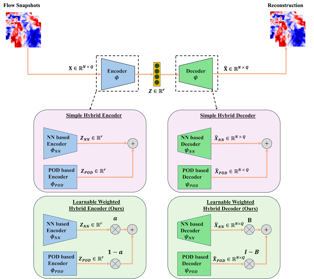
Figure 1: Architecture of the simple hybrid autoencoder and learnable weighted hybrid autoencoder.

3 Datasets and model setup

3.1 Kuramoto-Sivashinsky (KS)

The governing equation of the KS equation is $\frac{\partial u}{\partial t}+u\frac{\partial u}{\partial x}+\frac{\partial^{2}u}{\partial x^{2}}+\frac{\partial^{4}u}{\partial x^{4}}=0$, where $x\in[0,L_{x})$, $L_{x}=64\pi$, and periodic boundary conditions are assumed. The initial conditions comprise a sum of ten random sine and cosine waves $u(x,0)=\sum_{k=1}^{10}A_{k}\left(\sin\left(\frac{2\pi n_{k}x}{L_{x}}+\phi_{k}\right)+\cos\left(\frac{2\pi n_{k}x}{L_{x}}+\phi_{k}\right)\right)$, where $\forall k\in\{1,\ldots,10\},A_{k}\sim U(-1,1),\phi_{k}\sim U(0,2\pi)$, and wavenumber $n_{k}\sim U\{1,\ldots,6\}$, respectively. We employ Fourier decomposition in space and 2nd order Crank-Nicolson Adam-Bashforth semi-implicit finite difference scheme for temporal discretization. The data is generated for around 2000 time steps with a timestep of 0.01. Grid sizes of 512, 1024 and 2048 is used for the simulation. A few initial snapshots of the simulation that corresponds to transient phase are ignored.

For the NN encoder, we use a feedforward neural network with one hidden layers. Hyperbolic tangent function is used for activation in all layers except the last linear layer. The NN decoder is symmetric to the encoder. After shuffling, snapshot data is split into training and testing with 7:3 ratio. Before training, we standardize the data by subtracting the mean and dividing by the standard deviation. All models are trained for 40k epochs with a batch size of 64.

3.2 Homogeneous isotropic turbulence (HIT)

Direct numerical simulation data of forced homogeneous isotropic turbulence is obtained from Johns Hopkins turbulence database [18]. The dataset is generated by solving the forced Navier Stokes equation on a periodic cubic box using pseudo-spectral method. We interpolate the velocity field, $u(x,t)=(u_{x},u_{y},u_{z})\in\mathbb{R}^{3}$, from the original dataset of resolution $1024^{3}$ to grid sizes of $16^{3}$, $32^{3}$ and $64^{3}$ and extract the data from timestep 1 to 2048 with a stride of 16, resulting around 128 snapshots.

We choose a deep convolutional autoencoder [19] as the NN part of the proposed framework. The NN encoder starts with 4 hidden layers of convolution, each followed by Swish activation. The number of filters increase from 256 to 2048 by a factor of two every layer. Then we flatten last layer output and pass it through a linear layer to obtain the reduced space representation. The NN decoder is symmetric to the encoder. Dropout with a probability of 0.4 was used at each layer of the encoder and decoder except the output layer. Without shuffling, we systematically sample the dataset by selecting every alternate snapshot to curate the training and testing data, each comprising of 64 snapshots. All models are trained for 2k epochs with a batch size of 20.

4 Discussion

4.1 Generalization performance and convergence

To demonstrate the effectiveness of the proposed approach, we compare our model against three other methods: POD, vanilla deep autoencoder (AE), simple hybrid autoencoder, as autoencoders for the two chaotic PDE datasets in sections 3.1 and 3.2 with varying rank $r$ and resolution $N$. Sixteen ensembles of the model is trained by setting different random seeds. From fig. 2, both of the two hybrid approaches perform better than AE and POD. But the simple approach doesn’t maintain its convergence with increasing rank in contrast to our proposed approach. In addition, our approach shows orders of magnitude improvement in generalization as compared to any of the other methods. The simple and our learnable weighted hybrid approach give nearly the same test error at low ranks, but their gap increases multiple times with increasing rank. Surprisingly, such substantial improvement merely requires a negligible additional trainable parameters (i.e. $r+Q\ll N$), as shown in table 2. For this dataset the convergence of our approach follows a SVD like convergence, while the simple approach has a behaviour similar to AE.

Figure 2: Generalization performance of four models on 1D Kuramoto-Shivaskinsky dataset with varying rank $r$ and resolution $N$. X axis denotes the rank of the latent space and Y axis denotes the Mean Testing $L^{2}$ error. For each grid, rank, and method, the model is trained across 16 independent runs with varying random seed values. The results from these runs are averaged to compute the mean testing $L^{2}$ error. The convergence rate for POD and Learnable weighted hybrid approach is indicated in the legend as an exponent to $r$.

For the more challenging 3D HIT dataset, fig. 3 shows that our proposed approach continues to outperform the other three methods in terms of generalization, especially when the resolution increases (e.g., $32^{3},64^{3}$ as opposed to $16^{3}$). It is important to note that the simple approach shows little improvement over POD at resolution of $32^{3}$ or $64^{3}$ while our approach excels. Again, this highlights the important role of learnable weights in our hybrid approach. Additionally for this dataset, we study the impact of activation function on the reconstruction performance by utilizing ReLU activation function for the NN part of the auto-encoder. It is worth noting that the performance of both the AE and simple hybrid approaches exhibit noticeable variations when the activation function is changed. In contrast, our approach shows minimal changes in performance, demonstrating the robustness of the proposed framework. A further comparison among four models is shown in fig. 4, which visualizes the improvement in performance of our learnable weighted approach, especially on the small-scale turbulence. It is interesting to note that both POD and simple hybrid approach predicts a overly negative $u_{y}$ near the right middle. In addition, as shown in table 3, introducing such learnable weights has almost no overhead on the total number of parameters.

Figure 3: Generalization performance of four models on 3D homogeneous isotropic turbulence dataset with varying rank $r$ and resolution $N$. The testing $L^{2}$ error obtained using ReLU activation function is indicated using dashed lines. Similar to K-S case, 16 independent runs with varying random seed values are performed to obtain the mean testing $L^{2}$ error.

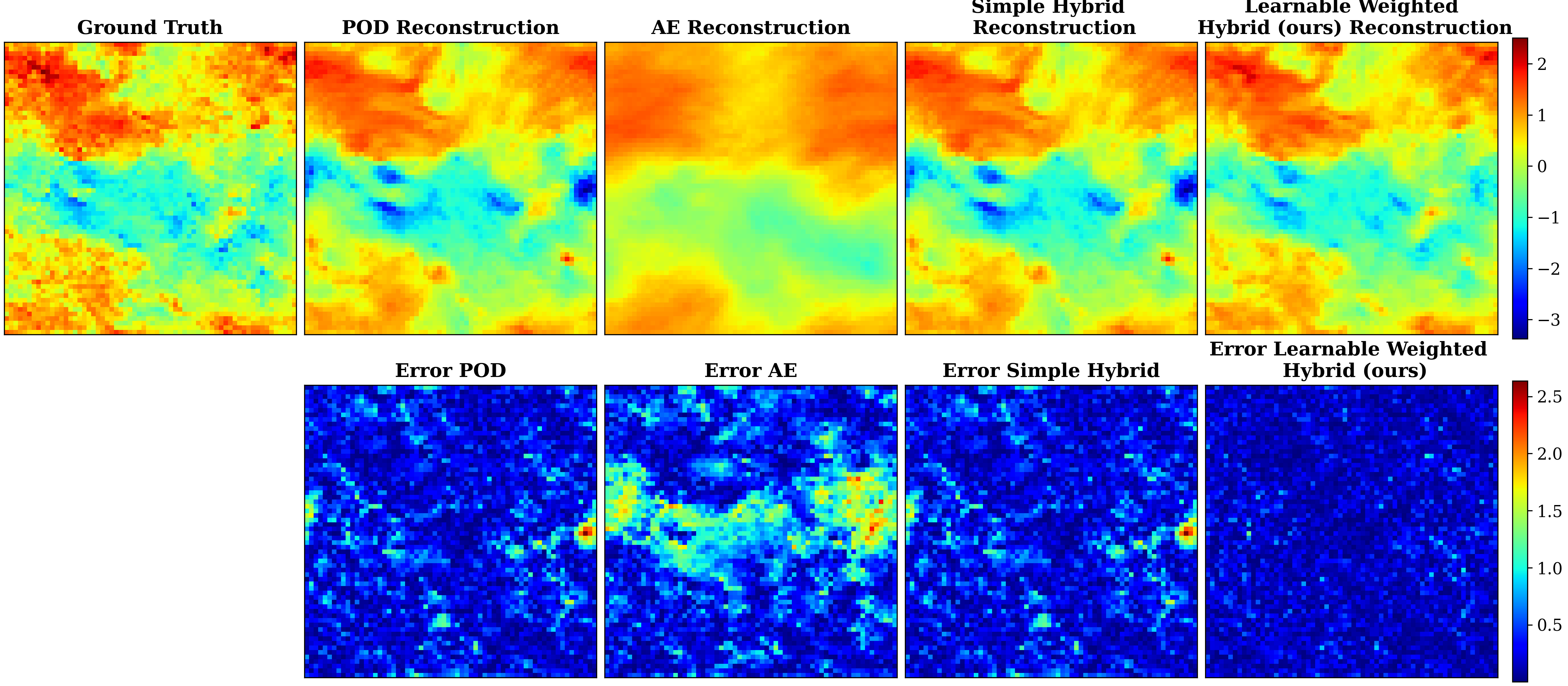
Figure 4: Generalization performance comparison on 3D HIT data at a resolution of $64^{3}$ and rank $r=5$, with a 2D slice of $u_{y}$. Left: $u_{y}$. Right: absolute error of $u_{y}$ between the reconstructed field and ground truth.

4.2 Sharpness and noise-robustness

Recent studies [20] in the deep learning community shows that sharpness of minima, which describes the sensitivity of model loss with respect to perturbations in the model parameters, is a promising quantity that correlates with the generalization performance of deep networks. Let $\mathcal{D}_{\textrm{train}}=\left\{(s_{1},g_{1}),\ldots,(s_{n},g_{n})\right\}$ be the training data, i.e., the set of feature $s$ and target $g$ pair, and $\ell_{i}(\mathbf{\Theta})$ be the loss of an NN model parametrized by weights $\mathbf{\Theta}$ and evaluated at $i$th training sample point $\left(s_{i},g_{i}\right)$. Afterwards, sharpness on a set of points $\mathcal{D}\subseteq\mathcal{D}_{\text{train}}$ can be defined as [21]: $\mathcal{S}(\mathbf{\Theta};\mathcal{D})\triangleq\max_{\|\delta\|_{2}\leq\rho}\frac{1}{|\mathcal{D}|}\sum_{i:\left(s_{i},g_{i}\right)\in\mathcal{D}}(\ell_{i}(\mathbf{\Theta}+\delta)-\ell_{i}(\mathbf{\Theta}))$ where $\delta$ is the perturbation introduced on the trainable parameters $\mathbf{\Theta}$ and $\rho$ refers to the perturbation radius. For example, table 1 shows sharpness and test error for a particular training instance of 3D HIT data with grid points $32^{3}$ and rank 5. Our proposed framework has 1000 times less sharpness when compared to the AE and simple hybrid approach. Since the sharpness of the minima is related to the resilience of the model in presence of noisy data, we evaluate the reconstruction performance of AE, learnable weighted, simple hybrid framework under noisy testing data. Models trained on noise-free data are tested on data which contains random normal noise with zero mean and standard deviation equal to $10\%$, $20\%$ and $30\%$ of the maximum velocity magnitude superimposed over the flow field.

Method	Sharpness	Testing $L^{2}$ Error
AE	$16.69\pm 0.9$	9.13
Simple Hybrid	$22.61\pm 0.82$	18.76
Learnable Weighted Hybrid (Ours)	$0.015\pm 0.001$	7.17

Table 1: Sharpness and testing $L^{2}$ error for three deep autoencoders with rank $r=5$ on the 3D HIT dataset at a resolution of $32^{3}$.

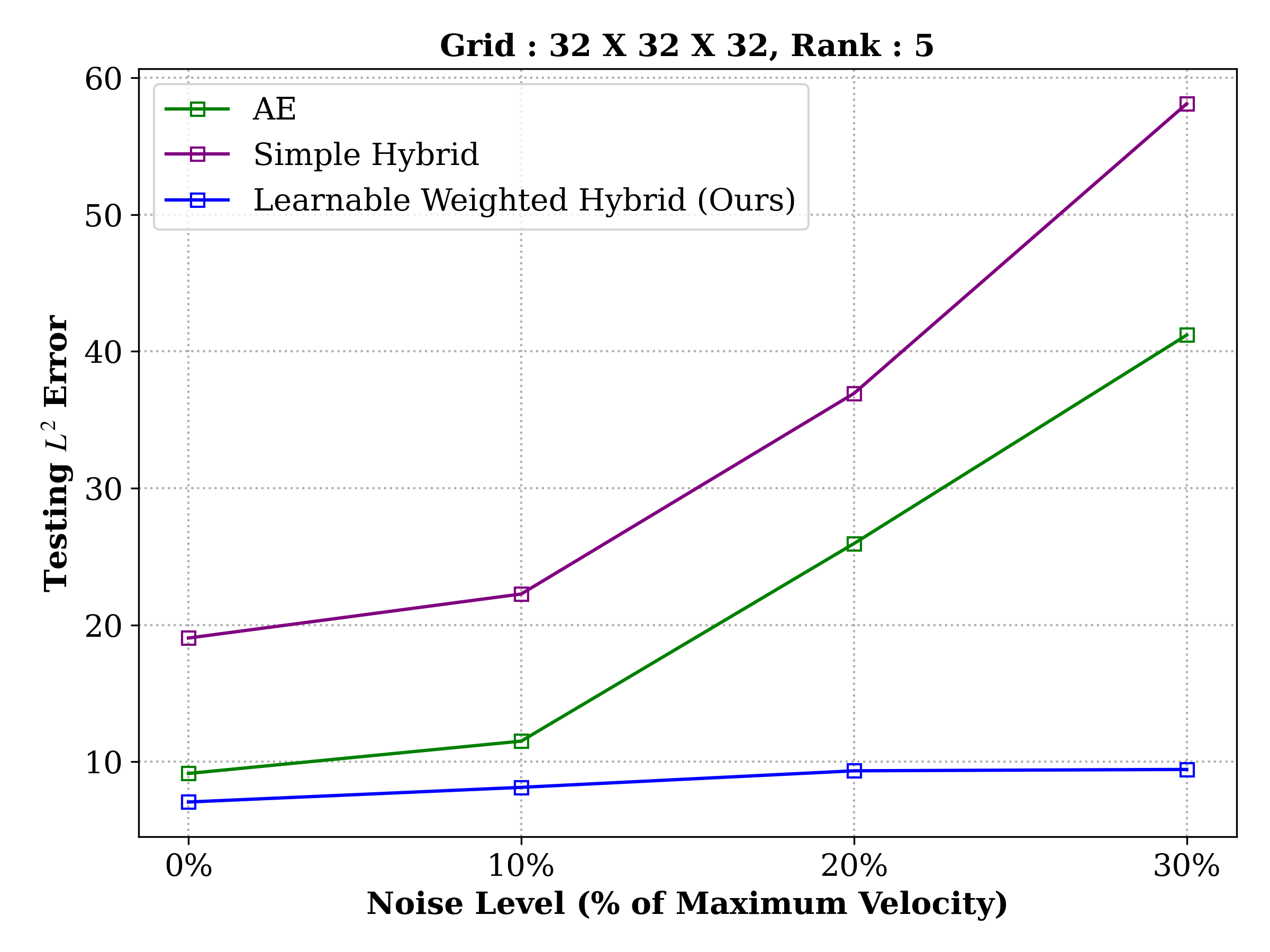
Figure 5: Comparison of testing $L^{2}$ error for varying noise level for three different deep autoencoder frameworks on 3D HIT dataset at resolution $32^{3}$ and rank $r=5$.

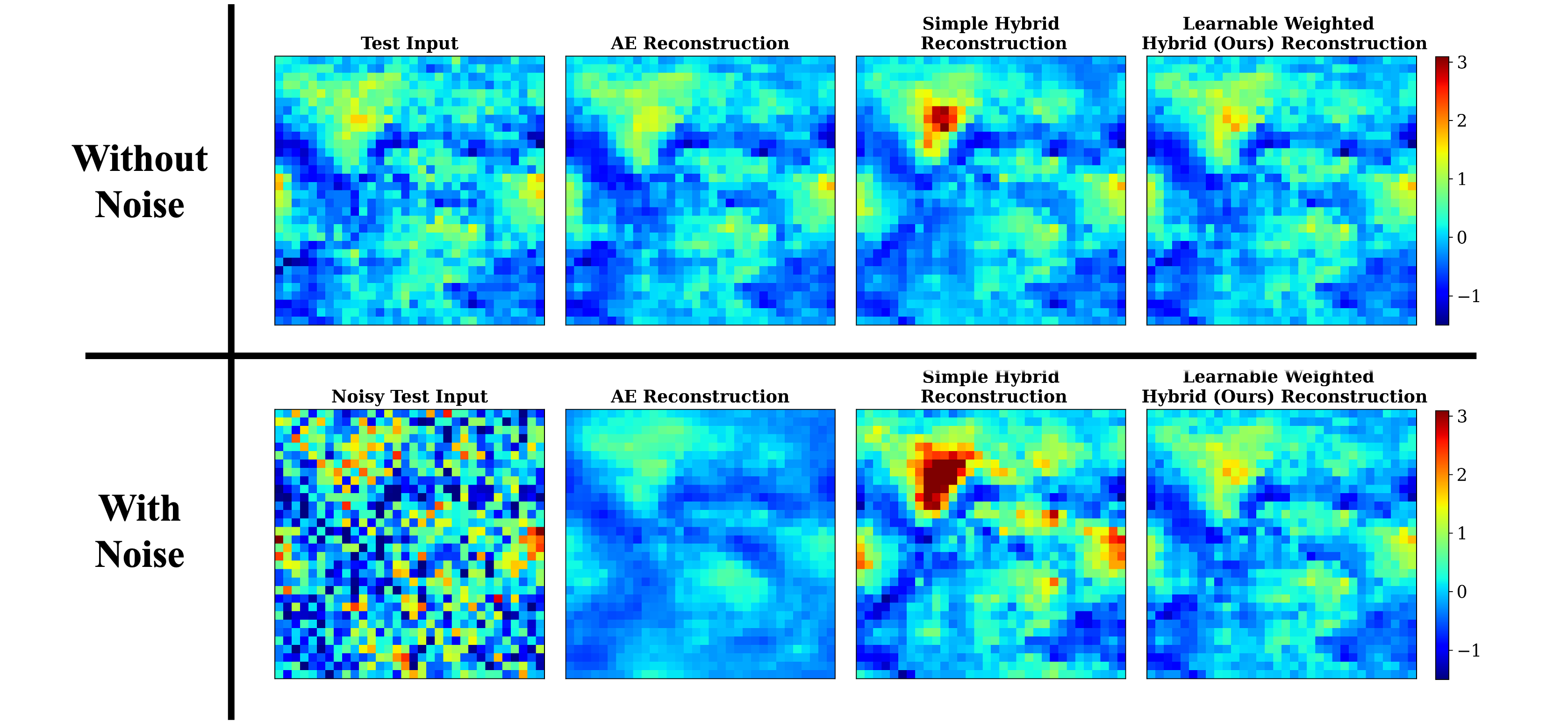
Figure 6: Comparison of the reconstruction performance of three different deep autoencoder frameworks on 3D HIT dataset at resolution $32^{3}$ and rank $r=5$. Left: noise free. Right: 30% noise level.

The reconstruction error for all models is shown in fig. 5. As noise level increases, there is a drastic increase in testing error for both AE and simple hybrid method, while our approach stays the same, demonstrating the robustness of this framework against noises in the unseen test data. A 2D slice of $u_{y}$ with and without 30% noise level is further visualized in fig. 6, which shows the improved robustness of our approach over other methods.

5 Conclusions

In this work, we present a novel deep autoencoder framework that demonstrates convergence properties akin to SVD. By incorporating a learnable weighted average between SVD and vanilla deep autoencoders (either feedforward or convolutional), our approach achieves SVD-like convergence as the rank increases. We validate the effectiveness of this framework on two challenging chaotic PDE datasets: the 1D Kuramoto-Sivashinsky and the 3D homogeneous isotropic turbulence. The results show that our learnable weighted hybrid autoencoder consistently achieves the lowest testing error and exhibits superior robustness to noisy data compared to other methods such as POD, vanilla deep autoencoders, and simple hybrid autoencoders. Remarkably, we find that our proposed approach leads to a minimum with a sharpness that is a thousand times smaller than that of other deep autoencoder frameworks, highlighting its potential for robust generalizable representation learning for complex PDE systems.

CRediT authorship contribution statement

Nithin Somasekharan: Data Curation (lead), Formal Analysis (lead), Investigation (lead), Software (lead), Visualization (lead), Writing – Original Draft Preparation (lead). Shaowu Pan: Conceptualization (lead), Funding Acquisition (lead), Methodology (lead), Supervision (lead), Writing – Review & Editing (lead), Project Administration (lead).

Appendix A Detailed comparison of numerical results

We summarize the detailed results of all numerical experiments conducted in this work in tables 2 and 3. Upon publication, the code will be made available at https://github.com/csml-rpi/deep-ae-with-svd-convergence.

Grid

Rank

Mean Train Error, $\mu$($\pm\sigma$)

Mean Test Error, $\mu$($\pm\sigma$)

Total Number of Model Parameters

POD

AE

Simple

Learnable Weighted

POD

AE

Simple

Learnable Weighted

POD

AE

Simple

Learnable Weighted

Hybrid

Hybrid (ours)

Hybrid

Hybrid (ours)

Hybrid

Hybrid (ours)

512

50

2.84e-01

2.54e-03

2.41e-04

1.62e-04

3.06e-01

2.73e-03

2.55e-04

1.92e-04

25,600

113,162

138,762

138,813

($\pm$ 1.92e-03)

($\pm$1.42e-03)

($\pm$6.07e-05)

($\pm$9.47e-06)

($\pm$4.80e-03)

($\pm$1.49e-03)

($\pm$5.96e-05)

($\pm$1.03e-05)

60

6.89e-02

1.68e-03

1.88e-04

1.59e-05

7.50e-02

1.76e-03

1.94e-04

1.96e-05

30,720

138,092

168,812

168,873

($\pm$ 4.92e-04)

($\pm$5.84e-04)

($\pm$7.35e-05)

($\pm$7.32e-07)

($\pm$1.47e-03)

($\pm$5.75e-04)

($\pm$7.38e-05)

($\pm$2.94e-06)

70

1.83e-02

1.75e-03

1.93e-04

2.73e-06

2.03e-02

1.79e-03

1.97e-04

3.55e-06

35,840

163,822

199,662

199,733

($\pm$ 1.37e-04)

($\pm$1.14e-03)

($\pm$1.26e-04)

($\pm$3.95e-07)

($\pm$3.67e-04)

($\pm$1.10e-03)

($\pm$1.28e-04)

($\pm$9.03e-07)

80

4.59e-03

2.07e-03

1.55e-04

1.02e-06

5.16e-03

2.22e-03

1.58e-04

1.39e-06

40,960

190,352

231,312

231,393

($\pm$ 2.95e-05)

($\pm$1.68e-03)

($\pm$4.62e-05)

($\pm$1.05e-07)

($\pm$8.78e-05)

($\pm$1.75e-03)

($\pm$4.72e-05)

($\pm$5.40e-07)

1024

50

3.18e-01

6.48e-03

3.01e-04

2.53e-04

3.41e-01

6.95e-03

3.20e-04

2.98e-04

51,200

216,074

267,274

267,325

($\pm$ 2.28e-03)

($\pm$2.53e-03)

($\pm$6.88e-05)

($\pm$2.29e-05)

($\pm$5.12e-03)

($\pm$2.49e-03)

($\pm$6.89e-05)

($\pm$2.29e-05)

60

8.75e-02

6.10e-03

2.14e-04

2.89e-05

9.53e-02

6.19e-03

2.22e-04

3.61e-05

61,440

261,484

322,924

322,985

($\pm$ 4.46e-04)

($\pm$7.01e-03)

($\pm$6.56e-05)

($\pm$3.29e-06)

($\pm$1.11e-03)

($\pm$6.43e-03)

($\pm$6.54e-05)

($\pm$5.84e-06)

70

2.21e-02

3.76e-03

2.25e-04

5.33e-06

2.46e-02

4.08e-03

2.30e-04

7.10e-06

71,680

307,694

379,374

379,445

($\pm$ 9.31e-05)

($\pm$2.64e-03)

($\pm$1.31e-04)

($\pm$1.31e-06)

($\pm$3.32e-04)

($\pm$2.72e-03)

($\pm$1.30e-04)

($\pm$2.38e-06)

80

5.86e-03

3.69e-03

2.23e-04

1.94e-06

6.58e-03

4.00e-03

2.26e-04

2.68e-06

81,920

354,704

436,624

436,705

($\pm$ 3.16e-05)

($\pm$2.34e-03)

($\pm$1.07e-04)

($\pm$1.54e-07)

($\pm$9.69e-05)

($\pm$2.34e-03)

($\pm$1.06e-04)

($\pm$8.49e-07)

2048

50

2.92e-01

1.62e-02

2.74e-04

2.36e-04

3.15e-01

1.82e-02

2.98e-04

2.80e-04

102,400

421,898

524,298

524,349

($\pm$ 2.34e-03)

($\pm$1.81e-02)

($\pm$7.71e-05)

($\pm$2.03e-05)

($\pm$5.32e-03)

($\pm$1.88e-02)

($\pm$8.97e-05)

($\pm$3.50e-05)

60

7.20e-02

9.93e-03

1.65e-04

3.39e-05

7.84e-02

1.14e-02

1.76e-04

4.35e-05

122,880

508,268

631,148

631,209

($\pm$ 4.95e-04)

($\pm$4.29e-03)

($\pm$2.48e-05)

($\pm$2.63e-06)

($\pm$1.31e-03)

($\pm$4.79e-03)

($\pm$2.31e-05)

($\pm$1.05e-05)

70

1.80e-02

7.65e-03

2.52e-04

1.21e-05

1.99e-02

9.18e-03

2.59e-04

1.61e-05

143,360

595,438

738,798

738,869

($\pm$ 9.85e-05)

($\pm$3.15e-03)

($\pm$7.35e-05)

($\pm$6.28e-07)

($\pm$3.20e-04)

($\pm$3.47e-03)

($\pm$7.46e-05)

($\pm$4.49e-06)

80

4.72e-03

9.62e-03

3.07e-04

9.23e-06

5.34e-03

1.12e-02

3.13e-04

1.23e-05

163,840

683,408

847,248

847,329

($\pm$ 3.99e-05)

($\pm$6.61e-03)

($\pm$2.34e-04)

($\pm$3.11e-07)

($\pm$1.54e-04)

($\pm$6.77e-03)

($\pm$2.30e-04)

($\pm$2.95e-06)

Table 2: Summary of training $L^{2}$ error, testing $L^{2}$ error, and the number of parameters for the four models trained on data with varying grid resolutions and ranks $r$ pertaining to 1D K-S case. The standard deviation of the error is indicated in parenthesis. The number of parameters for the hybrid approaches includes non-trainable POD parameters, which remain fixed throughout the optimization process and are not trainable.

Grid	Rank	Mean Train Error, $\mu$($\pm\sigma$)				Mean Test Error, $\mu$($\pm\sigma$)				Total Number of Model Parameters
		POD	AE	Simple	Learnable Weighted	POD	AE	Simple	Learnable Weighted	POD	AE	Simple	Learnable Weighted
				Hybrid	Hybrid (ours)			Hybrid	Hybrid (ours)			Hybrid	Hybrid (ours)
$16^{3}$	5	2.01e+01	1.05e+00	1.35e+00	1.76e+00	2.04e+01	5.74e+00	5.98e+00	5.48e+00	61,440	688,348,168	688,409,608	688,409,616
		($\pm$ 0.00)	($\pm$1.37e-01)	($\pm$1.13e-01)	($\pm$9.31e-02)	($\pm$0.00)	($\pm$3.13e-01)	($\pm$1.09e-01)	($\pm$6.44e-02)
	10	1.41e+01	9.71e-01	6.85e-01	9.02e-01	1.47e+01	5.53e+00	5.17e+00	5.22e+00	122,880	688,368,653	688,491,533	688,491,546
		($\pm$ 0.0)	($\pm$2.75e-01)	($\pm$6.05e-02)	($\pm$4.04e-02)	($\pm$0.0)	($\pm$1.11e-01)	($\pm$3.20e-02)	($\pm$3.49e-02)
	15	1.14e+01	8.76e-01	4.65e-01	6.35e-01	1.23e+01	5.47e+00	5.08e+00	5.20e+00	184,320	688,389,138	688,573,458	688,573,476
		($\pm$ 0.0)	($\pm$4.36e-02)	($\pm$2.43e-02)	($\pm$3.55e-02)	($\pm$0.00)	($\pm$1.02e-01)	($\pm$3.22e-02)	($\pm$3.59e-02)
	20	9.71e+00	8.96e-01	3.07e-01	5.06e-01	1.09e+01	5.49e+00	4.85e+00	5.21e+00	245,760	688,409,623	688,655,383	688,655,406
		($\pm$ 0.00)	($\pm$5.07e-02)	($\pm$1.90e-02)	($\pm$2.83e-02)	($\pm$0.00)	($\pm$6.92e-02)	($\pm$3.01e-02)	($\pm$3.14e-02)
$32^{3}$	5	2.02e+01	9.15e+00	1.84e+01	5.56e+00	2.04e+01	1.05e+01	1.87e+01	7.16e+00	491,520	688,505,864	688,997,384	688,997,392
		($\pm$ 0.00)	($\pm$1.10e+01)	($\pm$2.61e-01)	($\pm$1.03e-01)	($\pm$0.00)	($\pm$1.05e+01)	($\pm$2.34e-01)	($\pm$7.28e-02)
	10	1.42e+01	1.52e+01	1.23e+01	3.98e+00	1.47e+01	1.63e+01	1.32e+01	6.50e+00	983,040	688,669,709	689,652,749	689,652,762
		($\pm$ 0.00)	($\pm$1.74e+01)	($\pm$1.45e-01)	($\pm$6.67e-02)	($\pm$0.00)	($\pm$1.66e+01)	($\pm$1.27e-01)	($\pm$5.38e-02)
	15	1.15e+01	1.46e+01	9.18e+00	2.90e+00	1.22e+01	1.59e+01	1.06e+01	6.18e+00	1,474,560	688,833,554	690,308,114	690,308,132
		($\pm$ 0.00)	($\pm$1.76e+01)	($\pm$1.81e-01)	($\pm$5.54e-02)	($\pm$0.00)	($\pm$1.68e+01)	($\pm$1.55e-01)	($\pm$4.65e-02)
	20	9.78e+00	1.10e+01	6.91e+00	2.21e+00	1.08e+01	1.26e+01	8.86e+00	5.97e+00	1,966,080	688,997,399	690,963,479	690,963,502
		($\pm$ 0.00)	($\pm$1.52e+01)	($\pm$2.84e-01)	($\pm$4.70e-02)	($\pm$0.00)	($\pm$1.44e+01)	($\pm$1.55e-01)	($\pm$3.96e-02)
$64^{3}$	5	2.02e+01	2.89e+01	1.95e+01	9.00e+00	2.04e+01	2.89e+01	1.96e+01	9.53e+00	3,932,160	689,767,432	693,699,592	693,699,600
		($\pm$ 0.00)	($\pm$1.94e+01)	($\pm$1.53e-01)	($\pm$9.62e-02)	($\pm$0.00)	($\pm$1.91e+01)	($\pm$1.48e-01)	($\pm$9.27e-02)
	10	1.42e+01	2.50e+01	1.35e+01	7.01e+00	1.46e+01	2.52e+01	1.40e+01	7.95e+00	7,864,320	691,078,157	698,942,477	698,942,490
		($\pm$ 0.00)	($\pm$2.00e+01)	($\pm$1.22e-01)	($\pm$7.07e-02)	($\pm$0.00)	($\pm$1.96e+01)	($\pm$1.18e-01)	($\pm$6.18e-02)
	15	1.15e+01	1.65e+01	1.08e+01	5.59e+00	1.22e+01	1.69e+01	1.16e+01	7.01e+00	11,796,480	692,388,882	704,185,362	704,185,380
		($\pm$ 0.00)	($\pm$1.65e+01)	($\pm$1.79e-01)	($\pm$3.82e-02)	($\pm$0.00)	($\pm$1.62e+01)	($\pm$1.69e-01)	($\pm$3.63e-02)
	20	9.78e+00	1.94e+01	9.13e+00	4.54e+00	1.08e+01	1.97e+01	1.02e+01	6.45e+00	15,728,640	693,699,607	709,428,247	709,428,270
		($\pm$ 0.00)	($\pm$1.82e+01)	($\pm$9.70e-02)	($\pm$3.73e-02)	($\pm$0.00)	($\pm$1.78e+01)	($\pm$9.29e-02)	($\pm$3.39e-02)

Table 3: Summary of training $L^{2}$ error, testing $L^{2}$ error error, and number of parameters for the four models trained on data with varying resolutions $N$ and ranks $r$ pertaining to 3D HIT case.

References

- [1] A. E. Deane, I. G. Kevrekidis, G. E. Karniadakis, S. Orszag, Low-dimensional models for complex geometry flows: Application to grooved channels and circular cylinders, Physics of Fluids A: Fluid Dynamics 3 (10) (1991) 2337–2354.
- [2] L. Sirovich, Turbulence and the dynamics of coherent structures. i. coherent structures, Quarterly of applied mathematics 45 (3) (1987) 561–571.
- [3] J. Weller, E. Lombardi, M. Bergmann, A. Iollo, Numerical methods for low-order modeling of fluid flows based on pod, International Journal for Numerical Methods in Fluids 63 (2) (2010) 249–268.
- [4] S. Buoso, A. Manzoni, H. Alkadhi, V. Kurtcuoglu, Stabilized reduced-order models for unsteady incompressible flows in three-dimensional parametrized domains, Computers & Fluids 246 (2022) 105604.
- [5] G. E. Hinton, R. R. Salakhutdinov, Reducing the dimensionality of data with neural networks, science 313 (5786) (2006) 504–507.
- [6] B. Peherstorfer, Breaking the kolmogorov barrier with nonlinear model reduction, Notices of the American Mathematical Society 69 (5) (2022) 725–733.
- [7] S. E. Ahmed, O. San, Breaking the kolmogorov barrier in model reduction of fluid flows, Fluids 5 (1) (2020) 26.
- [8] M. Milano, P. Koumoutsakos, Neural network modeling for near wall turbulent flow, Journal of Computational Physics 182 (1) (2002) 1–26.
- [9] S. Pawar, S. Rahman, H. Vaddireddy, O. San, A. Rasheed, P. Vedula, A deep learning enabler for nonintrusive reduced order modeling of fluid flows, Physics of Fluids 31 (8) (2019) 085101.
- [10] B. Zhang, Nonlinear mode decomposition via physics-assimilated convolutional autoencoder for unsteady flows over an airfoil, Physics of Fluids 35 (9) (2023).
- [11] N. A. Raj, D. Tafti, N. Muralidhar, Comparison of reduced order models based on dynamic mode decomposition and deep learning for predicting chaotic flow in a random arrangement of cylinders, Physics of Fluids 35 (7) (2023).
- [12] K. Lee, K. T. Carlberg, Model reduction of dynamical systems on nonlinear manifolds using deep convolutional autoencoders, Journal of Computational Physics 404 (2020) 108973.
- [13] Z. Dar, J. Baiges, R. Codina, Artificial neural network based correction for reduced order models in computational fluid mechanics, Computer Methods in Applied Mechanics and Engineering 415 (2023) 116232.
- [14] J. Barnett, C. Farhat, Y. Maday, Neural-network-augmented projection-based model order reduction for mitigating the kolmogorov barrier to reducibility, Journal of Computational Physics 492 (2023) 112420.
- [15] K. He, X. Zhang, S. Ren, J. Sun, Delving deep into rectifiers: Surpassing human-level performance on imagenet classification, in: Proceedings of the IEEE international conference on computer vision, 2015, pp. 1026–1034.
- [16] S. Wang, B. Li, Y. Chen, P. Perdikaris, Piratenets: Physics-informed deep learning with residual adaptive networks, ArXiv abs/2402.00326 (2024).
- [17] R. L. Kosut, T.-S. Ho, H. Rabitz, Quantum system compression: A hamiltonian guided walk through hilbert space, Physical Review A 103 (1) (2021) 012406.
- [18] Y. Li, E. Perlman, M. Wan, Y. Yang, C. Meneveau, R. Burns, S. Chen, A. Szalay, G. Eyink, A public turbulence database cluster and applications to study lagrangian evolution of velocity increments in turbulence, Journal of Turbulence 9 (2008) N31. doi:10.1080/14685240802376389.
- [19] K. Fukami, T. Nakamura, K. Fukagata, Convolutional neural network based hierarchical autoencoder for nonlinear mode decomposition of fluid field data, Physics of Fluids 32 (9) (2020).
- [20] P. Foret, A. Kleiner, H. Mobahi, B. Neyshabur, Sharpness-aware minimization for efficiently improving generalization, in: ICLR Spotlight, 2021.
- [21] M. Andriushchenko, N. Flammarion, Towards understanding sharpness-aware minimization, in: International Conference on Machine Learning, PMLR, 2022, pp. 639–668.