Super-resolved anomalous diffusion:
deciphering the joint distribution of anomalous exponent and diffusion coefficient

Abstract

The molecular motion in heterogeneous media displays anomalous diffusion by the mean-squared displacement $\langle X^{2}(t)\rangle=2Dt^{\alpha}$. Motivated by experiments reporting populations of the anomalous diffusion parameters $\alpha$ and $D$, we aim to disentangle their respective contributions to the observed variability when this last is due to a true population of these parameters and when it arises due to finite-duration recordings. We introduce estimators of the anomalous diffusion parameters on the basis of the time-averaged mean squared displacement and study their statistical properties. By using a copula approach, we derive a formula for the joint density function of their estimations conditioned on their actual values. The methodology introduced is indeed universal, it is valid for any Gaussian process and can be applied to any quadratic time-averaged statistics. We also explain the experimentally reported relation $D\propto\exp(\alpha c_{1}+c_{2})$ for which we provide the exact expression. We finally compare our findings to numerical simulations of the fractional Brownian motion and quantify their accuracy by using the Hellinger distance.

Diffusion in heterogeneous media is relevant to physics, chemistry and biology. Particle dynamics in a heterogeneous system reflect the interaction between a particle and its environment. Physical features such as reaction rates and ergodicity breaking, as well as statistical features such as rare events and non-Markovianity, are intrinsically connected with the nature of the medium heterogeneity. Recent single particle tracking experiments in heterogeneous and crowded environments, such as biological cells, have reported anomalous diffusion [1, 2, 3, 4]. In brief, a diffusive process $X(t)$ is labeled as anomalous if its ensemble averaged mean-squared displacement (EAMSD) grows in time as a power-law function, i.e.,

$$\langle X^{2}(t)\rangle=2Dt^{\alpha}\,,$$ (1)

where $\alpha\in[0,2]$ is the anomalous exponent and $D\in[0,\infty)$ is the generalized diffusion coefficient (hereinafter simply called diffusion coefficient) with units $m^{2}s^{-\alpha}$ , and $\langle\cdot\rangle$ denotes the expectation value. Anomalous exponent $\alpha$ can vary due to a change in the viscoelastic properties of the medium or to regime-switching between passive and active motion [5]. Similarly, the diffusion coefficient $D$ can be affected by changes in viscosity, hydrodynamic radius, or even temperature.

The distribution of the anomalous exponents has been discussed in the context of dynamics of histone-like nucleoid-structuring proteins [6], and quantum dot dynamics in cell cytoplasm [7, 8, 9]. The distribution of the diffusion coefficients has been discussed in $\beta$-adrenergic receptor dynamics [10]. The joint distribution of anomalous exponent and diffusion coefficient has been studied in the diffusion of G proteins [11], intracellular quantum dots [12], $\kappa$-opioid receptor [13], membrane-less organelles in C. elegans embryos [14], nanobeads in clawfrog X. laevis egg extract [15], and endosomal dynamics [16]. Additionally, the correlation between anomalous exponent and diffusion coefficient shows, in some cases, similar patterns [9, 15, 14, 16] for which we provide here an explanation.

Since the analysis of individual trajectories from experimental data suggests that $\alpha$ and $D$ can be randomly distributed, we address here the problem of characterizing the conditional joint distribution of the estimated parameters $(\hat{\alpha}\,,\hat{D})$ given the expected pair $(\alpha\,,D)$. From the experimental point of view, the stochastic nature of the system and the finite duration of the experimental trajectories introduce errors in the estimation of the parameters. For an expected pair $(\alpha\,,D)$, each realization of the process yields values of the estimated parameters $(\hat{\alpha}\,,\hat{D})$ affected by random fluctuations and resulting in a probability density function (PDF) $p(\hat{\alpha},\hat{D})$. Shorter trajectories exacerbate these estimation errors. This introduces a ’resolution limit’ to the joint PDF of the estimated parameters. In fact, when the true physical parameters are randomly distributed, the joint PDF of the estimated parameters can be viewed as a convolution between the distribution of the physical parameters and that of the estimation errors. The additional difficulty here is that the error level itself depends on $\alpha$ and $D$. Moreover, $\hat{\alpha}$ and $\hat{D}$ are correlated due to the formulation of the mathematical estimators.

Theoretically, this is the framework of superstatistics [17] where, in addition to thermal noise, further randomness is provided by fluctuations of intensive quantities along particles’ trajectory or by distinct parameters’ values for each particle. Thus, we enable the identification of potential superstatistical anomalous diffusion models where both $\alpha$ and $D$ can be randomly distributed even in the case of short trajectories. Furthermore, since the fractional Brownian motion (fBm) turned out to be a good candidate for the underlying stochastic motion in many living systems [18, 19, 20], the superstatistical fBm is considered in this study as a prototypical case. Superstatistical fBm characterized by a population of diffusion coefficients has been formulated within the framework of the generalized grey Brownian motion [21, 22] and also checked against experimental literature [23, 24]. More mathematical aspects related to ergodicity breaking [25] and the generalized Fokker–Planck equation were also studied [26, 27]. Additionally, fBm with a random anomalous exponent (called Hurst exponent) was also studied [28, 29, 30, 31, 32], and intriguing phenomena such as accelerated diffusion and time-dependent persistence transitions were observed. Extensions of fBm, where the Hurst exponent behaves as a stationary random process, have also been discussed in mathematical studies [33, 34]. Finally, two-variable superstatistical fBm has been preliminary discussed in the literature [35].

Thus, in the following, first, we propose a general methodology for identifying the joint PDF $p(\hat{\alpha},\hat{D})$ and, later, while our methodology is valid for any ergodic Gaussian process, we show our methodology at work in the case of the fBm [36]. Finally, we discuss the accuracy of the approach as a function of trajectory length.

The joint PDF $p(\hat{\alpha},\hat{D})$ is determined by

$$p(\hat{\alpha},\hat{D})=\int_{0}^{2}d\alpha\int_{0}^{\infty}dD\,p(\hat{\alpha},\hat{D}|\alpha,D)p(\alpha,D)\,,$$ (2)

where $p(\hat{\alpha},\hat{D}|\alpha,D)$ is the joint conditional PDF of the estimated anomalous exponent and diffusion coefficient given the true values $\alpha$ and $D$, respectively. Note that the joint conditional distribution depends implicitly on the trajectory length and the lag times used in the fitting. When $\alpha=\alpha_{0}$ and $D=D_{0}$ are constant, then

$$p(\alpha,D)=\delta(\alpha-\alpha_{0})\delta(D-D_{0})\,,$$ (3)

where $\delta(\cdot)$ is the Dirac delta function.

We introduce now the time-averaged mean-squared displacement (TAMSD) $M_{N}(\tau)$ where $\tau=t/\Delta t$ and $\Delta t$ is the time elapsed between two consecutive position recordings. It is known that, if the process is ergodic then its expectation equals the EAMSD, i.e., $\langle M_{N}(\tau)\rangle=2D(\tau\Delta t)^{\alpha}$. We also report that our method can be formulated in terms of other time-averaged statistics, see, e.g., [37]. When applying a linear fitting of the log-log transformed TAMSD, the estimators of anomalous exponent and diffusion coefficient are given by

$$\hat{\alpha}=f\left(\mathbf{M_{N}}\right)=\frac{\sum_{i=1}^{\tau_{max}}\ln(\tau_{i})\ln\left(\frac{M_{N}(\tau_{i})}{M_{N}(1)}\right)}{\sum_{i=1}^{n}\ln(\tau_{i})^{2}}\,,$$ (4)

$$\hat{D}=g\left(\mathbf{M_{N}}\right)=\frac{1}{2}\exp\left(h\left(\mathbf{M_{N}}\right)-\hat{\alpha}B\right)\,,$$ (5)

where

$$h\left(\mathbf{M_{N}}\right)=\frac{1}{\tau_{max}}\sum_{\tau=1}^{\tau_{max}}\ln(M_{N}(\tau))\,,$$ (6)

and

$$B=\frac{1}{\tau_{max}}\sum_{\tau=1}^{\tau_{max}}\ln(\tau\Delta t)\,.$$ (7)

We observe that the estimator [38] given in Eq.  (4) is a function of the ratios $M_{N}(\tau_{i})/M_{N}(1)$ such that it is independent of both $D$ and $\Delta t$. In the above, $\tau_{max}$ is the maximum lag time used in the fitting procedure. For conciseness, we use the notation $\mathbf{M_{N}}=\{M_{N}(1),\ldots,M_{N}(\tau),\ldots,M_{N}(\tau_{max})\}$, which emphasizes the use of all the TAMSD values corresponding to the lag times $\tau=1,2,...,\tau_{max}$. The estimators in Eq. (4) and Eq. (5) are mathematical objects that do not share the physical limitations of $\alpha$ and $D$. One can show that the anomalous exponent estimator has an upper bound by considering the deterministic case with a constant speed $v$, where $M_{N}(\tau)=2v\tau^{2}$. This serves as a physical upper bound for the TAMSD when there is no possible acceleration. Any random perturbation of this ideal case would slow down space exploration, thus lowering the anomalous exponent. Therefore, we conclude $\hat{\alpha}\leq 2$. In turn, for a perfectly immobile particle, the TAMSD is $M_{N}(\tau)=0$ from which the estimator diverges $\hat{\alpha}_{min}=-\infty$. For what the diffusion coefficient is concerned, it holds $\hat{D}\in[0,\infty)$ as expected.

Let us first consider the random variable $\hat{Y}=\ln(\hat{D})$ whose expression is

$$\hat{Y}=k\left(\mathbf{M_{N}}\right)=h\left(\mathbf{M_{N}}\right)-\hat{\alpha}B\,.$$ (8)

It is well known that the joint PDF of two correlated random variables can be expressed through a bivariate Gaussian distribution under the condition of Gaussian marginal distributions linear correlations. However, if either or both of these conditions are not fulfilled this approach is not applicable. In this case, copula theory [39] is the generalized framework that allows one to express the joint PDF (also applicable to dimensions higher than 2). To build the joint PDF in a two-dimensional version, Sklar’s theorem [40] tells us that three ingredients are needed: the marginal distributions of both variables and their correlation structure. There are multiple types of correlation structures such as independent, linear (Gaussian copula), exponential, etc. In general, the marginal PDFs of $\hat{\alpha}$ and $\hat{Y}$ are not Gaussian; therefore, copula modeling is justified in the considered case. However, given Eq. (8), $\hat{Y}$ and $\hat{\alpha}$ are linearly correlated; therefore, we chose a Gaussian copula density to model their correlation structure. We can express the joint conditional PDF $p(\hat{\alpha},\hat{Y}|\alpha,D)$ as follows

$$p(\hat{\alpha},\hat{Y}|\alpha,D)=c(Q_{\hat{\alpha}}(\hat{\alpha}),Q_{\hat{Y}}(\hat{Y}),\rho)\,q_{\hat{\alpha}}(\hat{\alpha})\,q_{\hat{Y}}(\hat{Y})\,,$$ (9)

where $c(u,v,\rho)$ is the Gaussian copula density with correlation coefficient $\rho$, marginal cumulative distribution functions (CDFs) $Q_{\hat{\alpha}}(\hat{\alpha})$ and $Q_{\hat{Y}}(\hat{Y})$ of $\hat{\alpha}$ and $\hat{Y}$, respectively, and corresponding PDFs $q_{\hat{\alpha}}(\hat{\alpha})$ and $q_{\hat{Y}}(\hat{Y})$. For clarity, we omit for a while the conditional notation for the marginal PDFs, marginal CDFs, and moments of the estimators, although they are all implicitly conditional on $\alpha$ and $D$.

The formula for the Gaussian copula density is

$$c(u,v,\rho)=\frac{1}{\sqrt{1-\rho^{2}}}\exp\left(-\frac{\rho^{2}(x^{2}+y^{2})-2\rho xy}{2(1-\rho^{2})}\right)\,,$$ (10)

where $x=\Phi^{-1}(u)$, $y=\Phi^{-1}(v)$, and $\Phi^{-1}(\cdot)$ denotes the inverse of standard Gaussian CDF. In our case, the correlation coefficient $\rho$ in Eq. (10) is given by

$$\rho=\frac{\langle\hat{Y}^{*}\hat{\alpha}^{*}\rangle}{\sqrt{\langle(\hat{Y}^{*})^{2}\rangle\,\langle(\hat{\alpha}^{*})^{2}\rangle}}\,,$$ (11)

where $\hat{\alpha}^{*}=\hat{\alpha}-\langle\hat{\alpha}\rangle$, $\hat{Y}^{*}=\hat{Y}-\langle\hat{Y}\rangle$.

In Appendix B we present the computations of the expectation and covariance of the function of TAMSD which are crucial for computing the moments of $\hat{\alpha}$ and $\hat{Y}$. We obtain the expectations of $\hat{\alpha}$ and $\hat{D}$

$$\left\{\begin{array}[]{l}\langle\hat{\alpha}\rangle\approx\alpha+\frac{1}{2}Tr[\Lambda^{\top}\mathcal{D}^{2}f(\langle\mathbf{M_{N}}\rangle)],\\ \\ \langle\hat{Y}\rangle\approx Y+\frac{1}{2}Tr[\Lambda^{\top}\mathcal{D}^{2}k(\langle\mathbf{M_{N}}\rangle)],\end{array}\right.$$ (12)

where $\mathcal{D}^{2}f(\cdot)$ (resp. $\mathcal{D}^{2}k(\cdot)$) denotes the Hessian matrix of the function $f(\cdot)$ (resp. $k(\cdot)$) defined in Eq. (4) (resp. Eq. (8)) with respect to the variables $M_{N}(1),\ldots,M_{N}(\tau_{max})$. Moreover, $\Lambda$ is the covariance matrix of $\mathbf{M_{N}}$, see, Appendix A for more details. It should be noted that the expectations of the estimators yield the true values of $\alpha$ and $Y$ with corrections. The corrections depend on the covariance of TAMSD. When $N\to\infty$ but $\tau_{max}$ is fixed, the distribution of TAMSD converges to a Dirac delta function $\delta(x-\langle M_{N}(\tau)\rangle)$ and the covariance of TAMSD vanishes. Thus, the estimators $\hat{\alpha}$ and $\hat{Y}$ are asymptotically unbiased. However, at finite $N$ the corrections given in Eq. (12) should be taken into account. The first-order expansion of the functions $f(\cdot)$ and $k(\cdot)$ yields the approximate covariance and variances

$$\left\{\begin{array}[]{l}\langle(\hat{\alpha}^{*})^{2}\rangle\approx\nabla f(\langle\mathbf{M_{N}}\rangle)^{\top}\,\Lambda\,\nabla f(\langle\mathbf{M_{N}}\rangle),\\ \langle(\hat{Y}^{*})^{2}\rangle\approx\nabla k(\langle\mathbf{M_{N}}\rangle)^{\top}\,\Lambda\,\nabla k(\langle\mathbf{M_{N}}\rangle),\\ \langle\hat{Y}^{*}\hat{\alpha}^{*}\rangle\approx\nabla f(\langle\mathbf{M_{N}}\rangle)^{\top}\,\Lambda\,\nabla h(\langle\mathbf{M_{N}}\rangle)-\langle(\hat{\alpha}^{*})^{2}\rangle B,\end{array}\right.$$ (13)

where $\nabla f(\cdot)$ denotes the gradient vector of $f(\cdot)$ and conversely. The moments of estimators $\hat{\alpha}$ and $\hat{D}$ depend on the expectation $\langle M_{N}(\tau)\rangle$, covariance matrix $\Lambda$ of $M_{N}(\tau)$ which expressions can be obtained exactly

$$\left\{\begin{array}[]{l}\langle M_{N}(\tau)\rangle=Tr[R_{\tau}\Sigma]\\ \Lambda_{ij}=\langle{M_{N}(i)}^{*}{M_{N}(j)}^{*}\rangle=2Tr[\Sigma R_{i}\Sigma R_{j}],\end{array}\right.$$ (14)

where $\Sigma$ is the covariance matrix of the Gaussian process underlying the trajectories (see [42]), $R_{\tau}$ is the matrix of which entries are defined as [43]

$$R_{\tau}(n_{1},n_{2})=\frac{1}{N-\tau}(m_{n_{1}}\delta_{n_{1},n_{2}}-\delta_{|n_{1}-n_{2}|,\tau}),$$ (15)

where $\delta_{\cdot,\cdot}$ is the Kronecker delta, and

$$m_{k}=\left\{\begin{array}[]{ll}\left\{\begin{array}[]{cl}1&k\leq\tau\textrm{ or }k>N-\tau\\ 2&\tau<k\leq N-\tau\end{array}\right.&\tau\leq N/2\\ \left\{\begin{array}[]{cl}1&k\leq N-\tau\textrm{ or }k>\tau\\ 0&N-\tau<k\leq\tau\end{array}\right.&\tau>N/2.\end{array}\right.$$ (16)

Finally, we obtain a general expression for the joint conditional PDF of $\hat{\alpha}$ and $\hat{D}$ through the variable change $\hat{Y}=\ln(2\hat{D})$ from which

$$p(\hat{\alpha},\hat{D}|\alpha,D)=$$ (17)

$$c(Q_{\hat{\alpha}}(\hat{\alpha}),Q_{\hat{Y}}(\ln(2\hat{D})),\rho)\,q_{\hat{\alpha}}(\hat{\alpha})\,\frac{1}{\hat{D}}q_{\hat{Y}}(\ln(2\hat{D})).$$

Importantly, this formulation allows us to explain why single particle experiments [9, 15, 14, 16] consistently report the relationship $\hat{D}\propto\exp(\hat{\alpha}c_{1}+c_{2})$. We obtain the exact expression for this general relation. The linear correlation between $\hat{\alpha}$ and $\hat{Y}$ in conjunction with the identity $\hat{Y}=\ln(2D)$ implies

$$\hat{D}=\frac{1}{2}\exp\left[\kappa\,(\hat{\alpha}-\langle\hat{\alpha}\rangle)+\langle\hat{Y}\rangle\right],$$ (18)

where $\kappa=\langle\hat{\alpha}^{*}\hat{Y}^{*}\rangle/\langle(\hat{\alpha}^{*})^{2}\rangle$. The exponential behavior is a generic signature of performing a linear fitting in log-log scale, however, the parameters depend implicitly on $\alpha$ and $D$ thus reflecting the underlying physical process. This relation can be easily verified against experimental data.

As long as the anomalous exponent estimator is far enough from the upper bound, its marginal PDF is well approximated by a Gaussian distribution with mean $\langle\hat{\alpha}\rangle$ and variance $\langle({\hat{\alpha}}^{*})^{2}\rangle$ as shown in Fig. 1 (1.A-B). Therefore, following the $3\sigma$ rule, we can set a simple criterion for the validity of the Gaussian approximation

$$\langle\hat{\alpha}\rangle+3\sqrt{\langle({\hat{\alpha}}^{*})^{2}\rangle}<2\,.$$ (19)

The aforementioned condition can be readily confirmed using the experimental data. Specifically, given the number of trajectories obtained from the experiment, we initially estimate the anomalous exponent for each trajectory individually. Subsequently, the expectation $\langle\hat{\alpha}\rangle$ and the variance $\langle({\hat{\alpha}}^{*})^{2}\rangle$ in condition (19) are substituted with their empirical equivalents derived from the data.

When condition (19) is satisfied, then $\hat{Y}$ is also well approximated by a Gaussian distribution, see, Fig. 1 (2.A-C). When both marginal PDF of $\hat{\alpha}$ and $\hat{Y}$ are Gaussian, then Eq. (9) reduces to a bi-variate Gaussian distribution

$$p(\hat{\alpha},\hat{Y}|\alpha,D)=\frac{1}{2\pi\sqrt{det(\Sigma)}}\exp\left(-\frac{1}{2}V_{\hat{\alpha},\hat{Y}}^{\top}C^{-1}V_{\hat{\alpha},\hat{Y}}\right),$$ (20)

where

$$\begin{array}[]{ccc}V_{\hat{\alpha},\hat{Y}}=\left(\begin{array}[]{c}\hat{\alpha}-\langle\hat{\alpha}\rangle\\ \hat{Y}-\langle\hat{Y}\rangle\end{array}\right),&C=\left[\begin{array}[]{cc}\langle(\hat{\alpha}^{*})^{2}\rangle&\langle\hat{\alpha}^{*}\hat{Y}^{*}\rangle\\ \langle\hat{\alpha}^{*}\hat{Y}^{*}\rangle&\langle(\hat{Y}^{*})^{2}\rangle\end{array}\right].\end{array}$$ (21)

From the above, after the variable change $\hat{Y}=\ln(2\hat{D})$ we obtain

$$p(\hat{\alpha},\hat{D}|\alpha,D)=\frac{1}{2\hat{D}\pi\sqrt{det(C)}}\exp\left(-\frac{1}{2}V_{\hat{\alpha},\hat{D}}^{\top}C^{-1}V_{\hat{\alpha},\hat{D}}\right),$$ (22)

where

$$V_{\hat{\alpha},\hat{D}}=\left(\begin{array}[]{c}\hat{\alpha}-\langle\hat{\alpha}\rangle\\ \ln(2\hat{D})-\langle\hat{Y}\rangle\end{array}\right).$$ (23)

The joint conditional PDF given in Eq. (22) is a simple yet powerful approximation under condition (19). It is given in explicit form as the expectations of $\hat{\alpha}$ and $\hat{Y}$ and the elements of $C$ are given in Eq. (12) and Eq. (13). In such a case, by averaging over $\hat{\alpha}$, the marginal PDF of $\hat{D}$ conditioned on the true values $\alpha$ and $D$ is log-normal with the expectation

$$\langle\hat{D}\rangle\approx D+\frac{1}{2}Tr[\Lambda^{\top}\mathcal{D}^{2}g(\langle\mathbf{M_{N}}\rangle)],$$ (24)

where the function $g(\cdot)$ is defined in Eq. (5). The first-order approximation of the variance of $\hat{D}$ is as follows

$$\langle({\hat{D}}^{*})^{2}\rangle\approx\overrightarrow{\partial g(\langle\mathbf{M_{N}}\rangle)}\,\Lambda\,\overrightarrow{\partial g(\langle\mathbf{M_{N}}\rangle)}.$$ (25)

In turn, when the condition in Eq. (19) is not fulfilled, the marginal PDF of $\hat{\alpha}$ becomes skewed. In such a case we observe that other distributions may be more appropriate to describe the behavior of $\hat{\alpha}$. In our analysis, we use the scaled-shifted Beta distribution and show that it is more suitable in the considered case, as it can account for the upper bound, see Fig.  1 (1.A-C). In Appendix C, we show that this distribution can be parameterized by its expectation and variance while its skewness and kurtosis are encoded in the bounds $\hat{\alpha}_{min}$ and $\hat{\alpha}_{max}$ of the distribution. The conditional marginal PDF of $\hat{Y}$ becomes skewed and with positive normalized kurtosis; therefore, the Gaussian distribution is also not suitable for this case. In Fig. 1 (2.A-C)) we present the fitting by the Pearson type IV distribution [44, 45], which seems to be a good candidate for the PDF of $\hat{Y}$, at the additional cost of computing the skewness and kurtosis of the estimator, see, Appendix C for more details.

We check our analytical result with simulations of fBm. For clarity, we consider $p(\alpha,D)$ to be Dirac distributed (see Eq. (3)), however, through Eq. (2) the results hold for arbitrary $p(\alpha,D)$. In Fig. 1 (columns (1) and (2)), we present the histograms of estimators $\hat{\alpha}$ (1.A-C) and $\hat{Y}$ (2.A-C) obtained from simulated $M=10^{5}$ fBm trajectories of $N=100$ steps with $\Delta t=1$ and $\tau_{max}=5$. The anomalous exponent $\alpha=\{0.2,1,1.6\}$ for rows A, B, and C respectively. In each case, we assume $D=1$. Solid blue lines correspond to the theoretical curves based on the Gaussian approximations while the yellow lines correspond to the estimated Beta PDFs (in case of $\hat{\alpha}$) and Pearson IV PDF (in case of $\hat{Y}$).

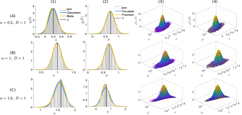
Figure 1: (1): Histograms of $\hat{\alpha}$ versus theoretical predictions for Gaussian (blue line) and Beta distribution (yellow line); (2): Histograms of $\hat{Y}$ versus theoretical prediction for Gaussian (blue line) and Pearson IV (yellow line). (3): histogram $p(\hat{\alpha},\hat{D})$ versus theory (magenta mesh) using Gaussian approximation of $\hat{\alpha}$ and $\hat{Y}$ from Eq. (22). (4): histogram $p(\hat{\alpha},\hat{D})$ versus theory (yellow mesh) using copula-based approach Eq. (17). All the empirical histograms were obtained from $M=10^{5}$ simulated fBm trajectories of $N=100$ steps with $\tau_{max}=5$ and $\alpha=\{0.2,1,1.6\}$ for rows A, B, C. In each case, we choose $D=1$ and $\Delta t=1$. For the yellow lines and mesh columns (1), (2), (4) the skewness and kurtosis used in marginal PDFs were obtained empirically.

In Fig. 1 (3.A-C) we present the joint PDF $p(\hat{\alpha},\hat{D})$ estimated with Gaussian approximation of $\hat{\alpha}$ and $\hat{Y}$ distributions for the simulated trajectories of fBm (see the caption of the figure for more details). The theoretical joint PDFs coincide with the empirical ones for smaller values of the $\alpha$ parameter. In Fig. 1 (4.A-C) we also present the joint PDF $p(\hat{\alpha},\hat{D})$ received using a copula-based approach. As can be seen, in such a case, the empirical and theoretical PDFs coincide also for large values of the anomalous exponent.

To examine how the length of the trajectory $N$ influences the Gaussian approximation of the joint PDF, in Fig. 2 we show the Hellinger distance [46] (represented as a function of $N$) between the theoretical joint PDF $p(\hat{\alpha},\hat{D})$ from Eq. (22) and the empirical joint PDF of $\hat{\alpha}$ and $\hat{D}$ obtained from the fBm trajectories for different values of $\alpha$ with $D=1$. The Hellinger distance, a measure of divergence (statistical distance), quantifies the difference between two probability distributions (in quadratic norm). For two probability distributions with PDFs $d_{1}(\cdot)$ and $d_{2}(\cdot)$, it is defined as follows

$$H(d_{1},d_{2})=\left(\int\left(\sqrt{d_{1}(x)}-\sqrt{d_{2}(x)}\right)^{2}dx\right)^{1/2}.$$ (26)

In practice, integral (26) is replaced by its empirical counterpart. In our study, the Hellinger distance is calculated in a two-dimensional context, where the densities $d_{1}(\cdot)$ and $d_{2}(\cdot)$ are the theoretical joint PDF $p(\hat{\alpha},\hat{D})$ and the empirical joint PDF of $\hat{\alpha}$ and $\hat{D}$, respectively. The analysis is conducted for $M=10^{6}$ fBm trajectories assuming $\Delta t=1$. As shown, the Gaussian approximation of the joint PDF $p(\hat{\alpha},\hat{D})$ is reasonable for $N=20$. From $N=30$ onwards, the Gaussian approximation is considered very accurate, except for large values of $\alpha$, which aligns with the results presented in Fig. 1.

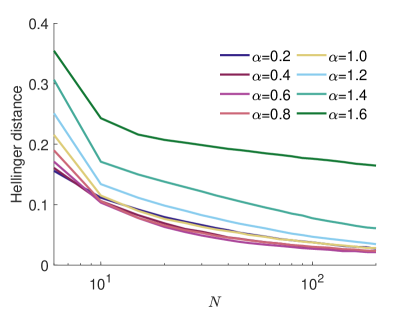
Figure 2: Hellinger distance as a function of the trajectories’ length $N$ between theoretical joint PDF $p(\hat{\alpha},\hat{D})$ (from Eq. (22)) and the empirical joint PDF of $\hat{\alpha}$ and $\hat{D}$ received from $M=10^{6}$ fBm-particles for different values of the anomalous exponent $\alpha$ with fixed $D=1$ and $\Delta t=1$.

In conclusion, we have presented the first complete characterization of the joint PDF of estimated anomalous diffusion parameters as a function of the underlying physical parameters. The proposed methodology is based on the copula theory for estimating the joint PDF and it performs well even for short trajectories ($\geq 30$ steps), which is critical for analyzing experimental data. It is known that reconstructing the joint distribution $p(\alpha,D)$ is crucial for correctly interpreting the dynamics and identifying changes in the physical parameters, particularly when following system perturbations (e.g., drug treatments in cellular biology). The conditional joint PDF can be characterized for any trajectory duration, therefore its knowledge enables a super-resolved joint PDF of the physical parameters beyond technical limitations due to trajectory duration. The PDF depends on the moments of the quadratic form, for which we provided analytical expressions in the case of general Gaussian processes. This framework enables the separation of variability in the estimated physical parameters, distinguishing between the intrinsic randomness of the trajectories and the distributional behavior of the physical parameters themselves. Our approach is general and it paves the way to derive the PDF of any sufficiently smooth function of a quadratic form in Gaussian random variables. The practical aspect of this study is the development of universal estimators for anomalous diffusion parameters, which provide a reliable way to separate true parameter variability from measurement limitations in experiments, improving the analysis of molecular motion in heterogeneous media and enabling more accurate interpretations of data in various contexts. Future work will extend this approach to account for experimental errors, which further complicate the parameter estimation.

Acknowledgments: The work of AW was supported by National Center of Science under Opus Grant 2020/37/B/HS4/00120 “Market risk model identification and validation using novel statistical, probabilistic, and machine learning tools”. GP and YL acknowledge the support by the Basque Government through the BERC 2022–2025 program and by the Ministry of Science and Innovation: BCAM Severo Ochoa accreditation CEX2021-001142-S / MICIN / AEI / 10.13039/501100011033.

Appendix A Appendix A : Mean and covariance of TAMSD

In general, the TAMSD can be computed as a quadratic form

$$M_{N}(\tau)=\mathbb{Y}_{N}^{\top}R_{\tau}\mathbb{Y}_{N},$$ (27)

where $R_{\tau}$ is a matrix of which elements are defined in Eq. (15) of the main text. This allows us to compute the moments and covariance of $M_{N}$ using the theory of quadratic forms [42].

We note $\Sigma$ the covariance matrix of a Gaussian process. In this case, we have

$$\langle M_{N}(\tau)\rangle=Tr[R_{\tau}\Sigma].$$ (28)

The covariance can also be computed explicitly

$$\langle M_{N}^{*}(i)M_{N}^{*}(j)\rangle=2Tr[\Sigma R_{i}\Sigma R_{j}].$$ (29)

Appendix B Appendix B : Statistical properties of functions of TAMSD

In this section, we establish the general formulas for the mean and variance of a function of $\mathbf{M_{N}}$.

B.1 Expectation of a function of TAMSD

Our goal is to find the expectation of $f(\mathbf{M_{N}})$ for a sufficiently smooth function $f(\cdot)$. This will allow us later to obtain statistics of the estimator of anomalous exponent and diffusion coefficient.

First, we define the centered TAMSD

$$M_{N}^{*}(\tau_{i})=M_{N}(\tau_{i})-\langle M_{N}(\tau_{i})\rangle.$$ (30)

Next, we proceed to a Taylor approximation around the means $\mathbf{\langle\mathbf{M_{N}}\rangle}$ up to the second order. The multidimensional Taylor expansion in matrix form reads

$$f\left(\mathbf{M_{N}}\right) \approx f\left(\mathbf{\langle M_{N}\rangle}\right)$$

$$+\mathbf{M_{N}^{*}}^{\top}\mathcal{D}f(\mathbf{\langle M_{N}\rangle})$$

$$+\frac{1}{2}\mathbf{M_{N}^{*}}^{\top}\mathcal{D}^{2}f(\mathbf{\langle M_{N}\rangle})\mathbf{M_{N}^{*}}$$

$$+\ldots,$$

where $\mathcal{D}f$ and $\mathcal{D}^{2}f$ are the gradient and the Hessian matrices, respectively, of $f(\cdot)$ with respect to the vector $\mathbf{M_{N}}$. Thus, we obtain the mean of the function $f(\cdot)$

$$\langle f\left(\mathbf{M_{N}}\right)\rangle$$

$$= f\left(\mathbf{\langle M_{N}\rangle}\right)+\frac{1}{2}\langle\mathbf{M_{N}^{*}}^{\top}\mathcal{D}^{2}f(\mathbf{\langle M_{N}\rangle})\mathbf{M_{N}^{*}}\rangle$$

$$= f\left(\mathbf{\langle M_{N}\rangle}\right)+\frac{1}{2}\sum_{i,j=1}^{\tau_{max}}\partial_{ij}f\left(\mathbf{\langle M_{N}\rangle}\right)\langle(M_{N}^{*}(\tau_{i})M_{N}^{*}(\tau_{j})\rangle.$$

Thus, it is clearly seen that the mean of the function $f(\cdot)$ is affected by the covariance of TAMSD.

Applying this result to the anomalous exponent estimator $\hat{\alpha}$ from Eq. (6) and to $\hat{Y}$ from Eq. (7) yields the expectations presented in Eq. (14) of the main text.

B.2 Covariance of two functions of TAMSD

Concerning the covariance calculation, for simplicity, we abandon the quadratic term in Eq. (B.1) to keep the linear approximation. The covariance of two functions $f(\cdot)$ and $g(\cdot)$ is

$$\langle f^{*}\left(\mathbf{M_{N}}\right)g^{*}\left(\mathbf{M_{N}}\right)\rangle$$ (33)

$$= \left\langle\left(\mathbf{M_{N}^{*}}^{\top}\mathcal{D}f(\mathbf{\langle M_{N}\rangle})\right)\left(\mathbf{M_{N}^{*}}^{\top}\mathcal{D}g(\mathbf{\langle M_{N}\rangle})\right)\right\rangle,$$

where the Gradient is a diagonal matrix and $f^{*}\left(\mathbf{M_{N}}\right)=f\left(\mathbf{M_{N}}\right)-\langle f\left(\mathbf{M_{N}}\right)\rangle$. We deduce

$$\langle f^{*}\left(\mathbf{M_{N}}\right)g^{*}\left(\mathbf{M_{N}}\right)\rangle$$

$$= \sum_{i,k}\partial_{i}f(\langle\mathbf{M_{N}}\rangle)\,\langle M_{N}^{*}(\tau_{i})M_{N}^{*}(\tau_{k})\rangle\,\partial_{k}g(\langle\mathbf{M_{N}}\rangle),$$

which can easily be computed as a quadratic form $\langle(f^{*}\left(\mathbf{M_{N}}\right)^{2}\rangle=u^{\top}\Lambda v$ with vectors elements $u_{i}=\partial_{i}f(\langle\mathbf{M_{N}}\rangle)$ and $v_{i}=\partial_{i}g(\langle\mathbf{M_{N}}\rangle)$ and the covariance matrix of TAMSD with elements $\Lambda_{ij}=\langle M_{N}^{*}(\tau_{i})M_{N}^{*}(\tau_{k})\rangle$. Applying this to one function being the anomalous exponent estimator from Eq. (6) and the other to be $\hat{Y}$ from Eq. (10) we obtain the covariance $\langle\hat{\alpha}^{*}\hat{Y}^{*}\rangle$covariance $\langle\hat{\alpha}^{*}\hat{Y}^{*}\rangle$ in Eq. (15).

The variance of a function $f(\cdot)$ of TAMSD can be computed in a very similar way

$$\langle(f^{*}\left(\mathbf{M_{N}}\right))^{2}\rangle$$

$$= \sum_{i,k}\partial_{i}f(\langle\mathbf{M_{N}}\rangle)\,\langle M_{N}^{*}(i)M_{N}^{*}(k)\rangle\,\partial_{k}f(\langle\mathbf{M_{N}}\rangle).$$

Appendix C Appendix C : Marginal distributions of $\hat{\alpha}$ and $\hat{Y}$ in the non-Gaussian case

C.1 Scaled-shifted beta distribution for $\hat{\alpha}$

The scaled-shifted beta distribution is a well-suited PDF to model the anomalous exponent estimator. It is a bounded distribution, therefore it can account for the upper bound $\hat{\alpha}<2$. Additionally, one of its limit cases is the Gaussian distribution, so it is compatible with the approximation of the anomalous exponent estimator when the condition in Eq. (20) of the main text is verified.

Suppose that $\hat{\alpha}$ is bounded such that $\hat{\alpha}_{min}\leq\hat{\alpha}\leq\hat{\alpha}_{max}$. The scaled-shifted beta distribution is

$$p(\hat{\alpha})=\frac{(\hat{\alpha}-\hat{\alpha}_{min})^{a-1}(\hat{\alpha}_{max}-\hat{\alpha})^{b-1}}{B(a,b)(\hat{\alpha}_{max}-\hat{\alpha}_{min})^{a+b-1}}.$$ (36)

An interesting parameterization for beta distribution is based on its mean and variance by setting $a=\phi\mu$ and $b=\phi(1-\mu)$, where

$$\mu=\frac{\langle\hat{\alpha}\rangle-\hat{\alpha}_{min}}{\hat{\alpha}_{max}-\hat{\alpha}_{min}},$$ (37)

and

$$\phi=(\hat{\alpha}_{max}-\hat{\alpha}_{min})^{2}\frac{\mu(1-\mu)}{\langle(\hat{\alpha}^{*})^{2}\rangle}-1.$$ (38)

The main interest of this parametrization is that $a$ and $b$ depend solely on the mean and variance of $\hat{\alpha}$. The bounds of the distribution $\alpha_{min}$ and $\alpha_{max}$ contain information about the skewness and kurtosis.

Because the estimator is not bounded on the interval $[0,2]$, one can use $\alpha_{min}<0$ and $\alpha_{max}>2$ to accomodate for the $\hat{\alpha}$ distribution. There are two option for determining. They can be either empirically estimated using

$$\left\{\begin{array}[]{l}\hat{\alpha}_{min}=min([0,min(\hat{\alpha})]),\\ \hat{\alpha}_{max}=2\end{array}\right.$$ (39)

or, they can be theoretically computed using the method of moments, which requires knowledge of the first 4 moments.

C.2 Pearson type IV distribution for $\hat{Y}$

The Pearson type IV distribution is a particular solution of the Pearson differential equation [44]

$$\frac{p(x)^{\prime}}{p(x)}+\frac{a+(x-\mu)}{b_{2}(x-\mu)^{2}+b_{1}(x-\mu)+b_{0}}=0,$$ (40)

of which particular solutions contain a large range of distributions as the Student’s t-distribution, Beta distribution, Gamma distribution, etc. The Pearson type IV distribution arose as a solution of this equation, it is less known than its other counterparts and is characterized by a high excess kurtosis and low skewness. For $b_{1}^{2}-4b_{2}b_{0}<0$, after making the change of variable variable $y=x+\frac{b_{1}}{2b_{2}}$, the solution is

$$p(y)\propto\left(1+\frac{y^{2}}{\alpha^{2}}\right)^{-m}\exp\left(-\nu\,\textrm{arctan}\left(\frac{y}{\alpha}\right)\right),$$ (41)

where $m=1/(2b_{2})$, $\nu=-\frac{2b_{2}a-b_{1}}{2b_{2}^{2}\alpha}$, and $\alpha=\frac{\sqrt{4b_{2}b_{0}-b_{1}^{2}}}{2b_{2}}$. The parameters can be fitted using a maximum likelihood approach [45] or by moment matching method using the expectation, variance, skewness, and kurtosis.

References

- S. and C. [2005] B. D. S. and F. C., Biophys. J. 89, 2960 (2005).
- Szymanski and Weiss [2009a] J. Szymanski and M. Weiss, Phys. Rev. Lett. 103, 038102 (2009a).
- Bronstein et al. [2009] I. Bronstein, Y. Israel, E. Kepten, S. Mai, Y. Shav-Tal, E. Barkai, and Y. Garini, Phys. Rev. Lett. 103, 018102 (2009).
- Höfling and Franosch [2013] F. Höfling and T. Franosch, Rep. Prog. Phys. 76, 046602 (2013).
- Arcizet et al. [2008] D. Arcizet, B. Meier, E. Sackmann, J. O. Rädler, and D. Heinrich, Phys. Rev. Lett. 101, 248103 (2008).
- Sadoon and Wang [2018] A. A. Sadoon and Y. Wang, Phys. Rev. E 98, 042411 (2018).
- Sabri et al. [2020] A. Sabri, X. Xu, D. Krapf, and M. Weiss, Phys. Rev. Lett. 125, 058101 (2020).
- Janczura et al. [2021] J. Janczura, M. Balcerek, K. Burnecki, A. Sabri, M. Weiss, and D. Krapf, New J. Phys. 23, 053018 (2021).
- Cherstvy et al. [2019] A. G. Cherstvy, S. Thapa, C. E. Wagner, and R. Metzler, Soft Matter 15, 2526 (2019).
- Grimes et al. [2023] J. Grimes, Z. Koszegi, Y. Lanoiselée, T. Miljus, S. O’Brien, T. Stepniewski, B. Medel-Lacruz, M. Baidya, M. Makarova, R. Mistry, J. Goulding, J. Drube, C. Hoffmann, D. Owen, A. Shukla, J. Selent, S. Hill, and D. Calebiro, Cell 186, 2238 (2023).
- Sungkaworn et al. [2017] T. Sungkaworn, M. Jobin, K. Burnecki, A. Weron, M. J. Lohse, and D. Calebiro, Nature 550, 543 (2017).
- Etoc et al. [2018] F. Etoc, E. Balloul, C. Vicario, D. Normanno, A. Liße Domenik, Sittner, J. Piehler, M. Dahan, and M. Coppey, Nat. Mater. 17, 740 (2018).
- Drakopoulos et al. [2020] A. Drakopoulos, Z. Koszegi, Y. Lanoiselée, H. Hübner, P. Gmeiner, D. Calebiro, and M. Decker, J. Med. Chem. 63, 3596 (2020).
- Benelli and Weiss [2021] R. Benelli and M. Weiss, New J. Phys 23, 063072 (2021).
- Speckner and Weiss [2021] K. Speckner and M. Weiss, Entropy 23, 892 (2021).
- Korabel et al. [2021a] N. Korabel, D. Han, A. Taloni, G. Pagnini, S. Fedotov, V. Allan, and T. A. Waigh, Entropy 23, 958 (2021a).
- Beck and Cohen [2003] C. Beck and E. G. D. Cohen, Physica A 322, 267 (2003).
- Magdziarz et al. [2009] M. Magdziarz, A. Weron, K. Burnecki, and J. Klafter, Phys. Rev. Lett. 103, 180602 (2009).
- Szymanski and Weiss [2009b] J. Szymanski and M. Weiss, Phys. Rev. Lett. 103, 038102 (2009b).
- Weiss [2013] M. Weiss, Phys. Rev. E 88, 010101(R) (2013).
- Mura and Pagnini [2008] A. Mura and G. Pagnini, J. Phys. A: Math. Theor: Math. Theor 41, 285003 (2008).
- Pagnini and Paradisi [2016] G. Pagnini and P. Paradisi, Fract. Calc. Appl. Anal. 19, 408 (2016).
- Maćkała and Magdziarz [2019] A. Maćkała and M. Magdziarz, Phys. Rev. E 99, 012143 (2019).
- Runfola et al. [2022] C. Runfola, S. Vitali, and G. Pagnini, R. Soc. Open Sci. 9, 221141 (2022).
- Molina-García et al. [2016] D. Molina-García, T. M. Pham, P. Paradisi, C. Manzo, and G. Pagnini, Phys. Rev. E 94, 052147 (2016).
- Pagnini [2012] G. Pagnini, Fract. Calc. Appl. Anal. 15, 117 (2012).
- Runfola and Pagnini [2024] C. Runfola and G. Pagnini, Physica D 467, 134247 (2024).
- Balcerek et al. [2022] M. Balcerek, K. Burnecki, S. Thapa, A. Wyłomańska, and A. V. Chechkin, Chaos 32, 093114 (2022).
- Han et al. [2020] D. Han, N. Korabel, R. Chen, M. Johnston, A. Gavrilova, V. J. Allan, S. Fedotov, and T. A. Waigh, ELife 9, e52224 (2020).
- Korabel et al. [2021b] N. Korabel, D. Han, A. Taloni, G. Pagnini, S. Fedotov, V. Allan, and T. A. Waigh, Entropy 23, 958 (2021b).
- Balcerek et al. [2023] M. Balcerek, A. Wyłomańska, K. Burnecki, R. Metzler, and D. Krapf, New J. Phys. 25, 103031 (2023).
- Wang et al. [2023] W. Wang, M. Balcerek, K. Burnecki, A. V. Chechkin, S. Janušonis, J. Slezak, T. Vojta, A. Wyłomańska, and R. Metzler, Phys. Rev. Res. 5, L032025 (2023).
- Lévy-Véhel and Peltier [1995] J. Lévy-Véhel and R. F. Peltier, Rapport de recherche de l’INRIA 2645, 10.1063/5.0201436 (1995).
- Ayache and Taqqu [2005] A. Ayache and M. S. Taqqu, Publicacions Matemàtiques 49, 459 (2005).
- Itto and Beck [2021] Y. Itto and C. Beck, J. R. Soc. Interface 18, 20200927 (2021).
- Beran et al. [2016] J. Beran, Y. Feng, S. Ghosh, and R. Kulik, Long-Memory Processes (Springer, 2016).
- Maraj et al. [2020] K. Maraj, D. Szarek, G. Sikora, M. Balcerek, A. Wyłomańska, and I. Jabłoński, Meas.: Sens. 7-9, 100017 (2020).
- Sikora et al. [2017] G. Sikora, M. Teuerle, A. Wyłomańska, and D. Grebenkov, Phys. Rev. E 96, 022132 (2017).
- Durante and Sempi [2016] F. Durante and C. Sempi, Principles of Copula Theory (Chapman & Hall, 2016).
- Nelsen [2013] R. Nelsen, An Introduction to Copulas (Springer Science in Statistics, 2013).
- [41] See Supplemental Material at URL-will-be-inserted-by-publisher.
- Magnus [1978] J. R. Magnus, Stat. Neerl. 32, 201 (1978), https://onlinelibrary.wiley.com/doi/pdf/10.1111/j.1467-9574.1978.tb01399.x .
- Grebenkov [2011] D. S. Grebenkov, Phys. Rev. E 83, 061117 (2011).
- Pearson and Henrici [1895] K. Pearson and O. M. F. E. Henrici, Phil. Trans. Roy. Soc. London. 186, 343 (1895), https://royalsocietypublishing.org/doi/pdf/10.1098/rsta.1895.0010 .
- Nagahara [1999] Y. Nagahara, Stat. & Prob. Lett. 43, 251 (1999).
- Csiszar and Shields [2004] I. Csiszar and P. Shields, Information Theory and Statistics: A Tutorial (Foundations and Trends in Communications and Information) (Now Publishers Inc., 2004).