Stability of equilibriums and bifurcation analysis of two-dimensional autonomous competitive Lotka-Volterra dynamical system
Abstract. A detailed analysis of the stability of equilibriums and bifurcations of the two-dimensional autonomous competitive Lotka-Volterra dynamical system is performed. Necessary and sufficient conditions are determined for equilibriums (without the origin) to be asymptotically stable or unstable on . Necessary and sufficient conditions are determined so that the observed dynamical system has no equilibriums in . All results are presented in five tables and five figures. We also found that four transcritical bifurcations occur in the observed dynamical system if it is analyzed on .
2020 Mathematics Subject Classification: 34A34; 34C23; 37C75.
Keywords and phrases: Lotka-Volterra; dynamical systems; stability; equilibriums; bifurcations.
1 Introduction
In this paper, we analyze the stability of equilibriums and bifurcations of a two-dimensional autonomous competitive Lotka-Volterra dynamical system
| (1.1) |
where is the density of species at a given time , is the inherent growth rate of species , is the effect that species has on species , for and , while for we have self-interacting terms , . In the absence of competition, the observed dynamical system (1.1) consists of two logistic equations (one for each species), with carrying capacity , for . Since the dynamical system (1.1) is competitive, we assume that and , for every . The reason for this is the assumed harmfulness of interspecies interactions, which directly implies , for every and . Moreover, the self-regulation of each species implies , for every . Moreover , because it is also assumed that the inherent growth rate of species is positive in the absence of competition, unless has the value (its carrying capacity), for .
Competitive dynamical systems were introduced by Lotka and Volterra (see [6, 9]). The stability of equilibriums of the autonomous Lotka-Volterra competitive model is analyzed in various literature (see, e.g. [4, 8, 5]). In [10] relationship between the coefficients and can be found so that the system (1.1), which has no equilibrium in , has an asymptotically stable equilibrium on one axis, while an unstable equilibrium lies on the other axes. These conditions are also generalized for the -dimensional case of the system (1.1) in [10], and [2]. Other papers dealing with suitable conditions for the two-dimensional and -dimensional non-autonomous Lotka-Volterra competition model are [1] and [3], respectively.
The importance of this work lies in the fact that all possible cases concerning the stability of equilibriums of the autonomous Lotka-Volterra competitive model are discussed here in detail, which to our knowledge has not been done anywhere else in the literature in this way. The new results of this paper concern the improvement of several results from [10], specifically the determination of necessary and sufficient conditions for equilibriums (without the origin) to be asymptotically stable or unstable in , as well as the determination of necessary and sufficient conditions for the observed dynamical system to have no equilibriums in . Furthermore, we have concluded that four transcritical bifurcations occur in the observed dynamical system if it is analyzed on , and we have determined the conditions under which these bifurcations occur. To our knowledge, these are also new results of this paper.
In Section 2 we analyze in detail the stability of equilibriums of the system (1.1). We assume that and that the main determinant or the minor determinants of the system (1.1) can be zero. This leads to some non-hyperbolic equilibriums and bifurcations. We note that in [7] only the stability of equilibriums of the system (1.1) for and for all non-zero determinants of this system was studied. This analysis can also be found in our paper in Section 2.1.1, but with a new notation that is more suitable for generalization to higher dimensions. In Section 3 we have improved several two-dimensional versions of the theorems from the paper [10], in particular with respect to sufficient and necessary conditions for equilibriums of the system (1.1) lying on the axes to be asymptotically stable or an unstable equilibriums. In Section 4 we present a bifurcation analysis of the dynamical system (1.1).
First we introduce the following notation. For the determinant of the matrix of the system (1.1) and the corresponding minors, we introduce the following notation
| (1.2) |
From (1.2) we can conclude that the number of different indices of the determinant indicates the order of this determinant as well as the elements on its main diagonal. The indices of the determinant of the matrix of the system (1.1) show that it is the second-order determinant whose elements on the main diagonal are and . Furthermore, the indices of the minors , where denote the second-order determinant whose elements on the main diagonal are (position ) and (position ). This notation is very useful for calculating the coordinates of the equilibriums of the system and their eigenvalues, as well as for generalizations to higher dimensions.
The following notation applies to Tables 1-5: U denotes an unstable equilibrium, AS represents an asymptotically stable equilibrium, SS stands for a semi-stable equilibrium and NI stands for a non-isolated equilibrium.
In all figures in our paper, we have colored the points representing unstable equilibriums in yellow, asymptotically stable equilibriums are colored red, semi-stable equilibriums are colored orange and non-isolated equilibriums are colored pink.
2 Stability analysis of the equilibriums
We consider two cases, depending on whether is zero or not.
2.1 Case
The number of equilibriums and their stability depend on the signs of , and . We analyze the following cases.
2.1.1 Case and
If , we have four different equilibriums of system (1.1), labelled , , and . Otherwise we would have three equilibriums of system (1.1), , and , since equilibrium would not lie in the first quadrant. We note that the conditions and ensure that the eigenvalues of the Jacobian matrix in our equilibriums , have non-zero real parts, as we will see in the following text. Consequently, our equilibriums are hyperbolic and therefore we can discuss their stability in the framework of the corresponding linearization of the dynamical system (1.1), because the Hartman–Grobman theorem provides us topological equivalence between a nonlinear dynamical system and its linearization in the neighbourhood of the hyperbolic equilibrium. Now we investigate the stability of all equilibriums.
The equilibrium . The eigenvalues of the Jacobian matrix at are , for . Since for every , we conclude that is an unstable node (unstable equilibrium).
The equilibrium . The eigenvalues of the Jacobian matrix at are , and . If , then is a stable node (asymptotically stable equilibrium). Otherwise, i.e. if , is therefore a saddle (unstable equilibrium).
The equilibrium . We note that the eigenvalues of the Jacobian matrix for are and , . We conclude that is a stable node (asymptotically stable equilibrium) if . If , then is a saddle point (unstable equilibrium).
The equilibrium . The situation is a little complicated in this case. As we have already mentioned, the coordinates of must be positive in order to lie in the first quadrant, i.e. it must be . If we denote the coordinates of by and , the Jacobian determinant at is
| (2.1) |
since and . Furthermore
| (2.2) |
from which we obtain that the characteristic polynomial of the matrix is . From (2.2) we conclude that is a stable node (asymptotically stable equilibrium) if and and . If and and , is a saddle (unstable equilibrium).
To summarize, is an unstable node (unstable equilibrium), while the stability of equilibrium depends solely on the sign of , the stability of equilibrium depends solely on the sign of , while the existence and stability of equilibrium depend on the signs of , and . The results are shown in Table 1.
| eq. |
|
|
|
|
|
|---|---|---|---|---|---|
| U (u. node) | U (u. node) | not possible case | U (u. node) | ||
| U (saddle) | U (saddle) | AS (s. node) | |||
| AS (s. node) | U (saddle) | U (saddle) | |||
| not exist | AS (s. node) | not exist | |||
| U (u. node) | not possible case | U (u. node) | U (u. node) | ||
| U (saddle) | AS (s. node) | AS (s. node) | |||
| AS (s. node) | AS (s. node) | U (saddle) | |||
| not exist | U (saddle) | not exist |
The case from Table 1, in which , , is not possible. If this were possible, then we would have
| (2.3) |
If we multiply the first inequality from (2.3) by and use the third inequality from (2.3), we get , which contradicts the second inequality from (2.3). The case that , , is also not possible.
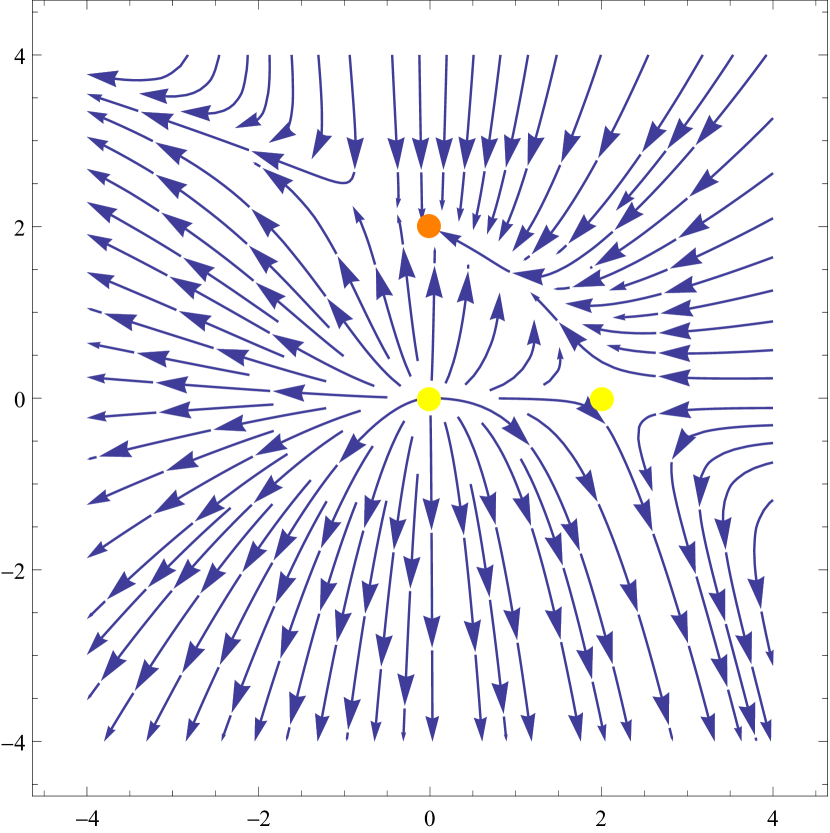
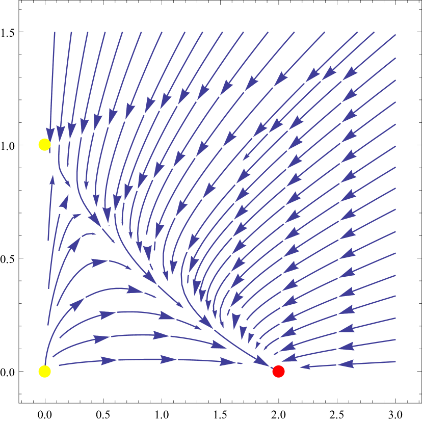
We conclude from Table 1 that cases with , , and , , , have the same qualitative dynamical properties, as well as the cases , , and , , . Therefore, in this section we have four qualitatively different phase portraits of the system (1.1). They are shown in Figures 1 and 2.
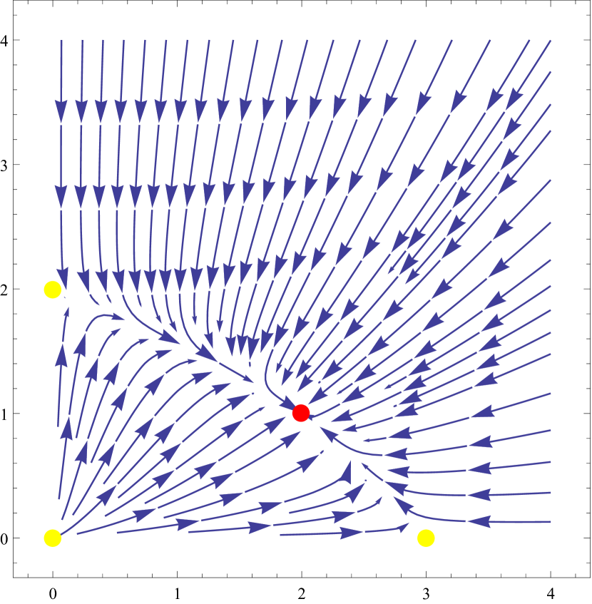
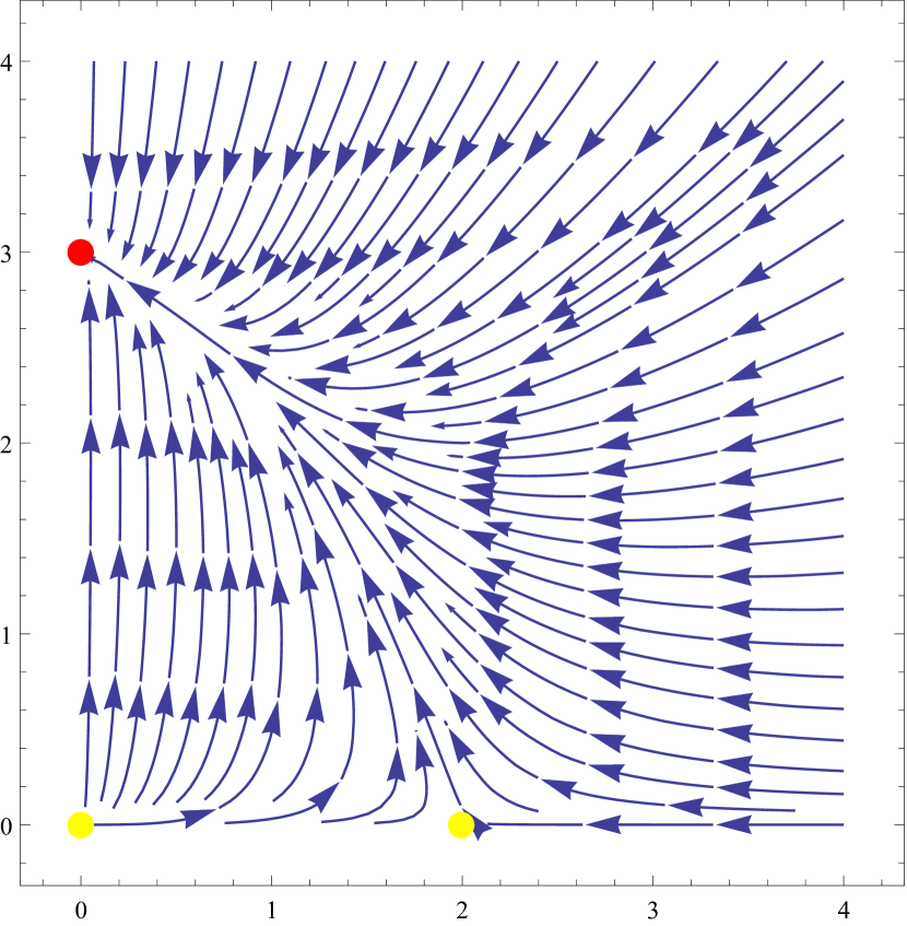
In Figures 1(a) and 1(b), the equilibrium at the origin is an unstable node, while the equilibrium is a saddle. In Figures 1(a) and 2(a), equilibrium is a saddle, while in Figures 1(b) and 2(b) it is a stable node. Equilibrium in Figure 1(a) is a stable node, while in Figure 2(b) is a saddle.
2.1.2 Case and
Since , we directly conclude that the first coordinate of is zero and that . Substituting into , we conclude that . Furthermore, the second coordinate of is , , from which it follows that the equilibrium coincides with and that . The equilibriums and are hyperbolic and their nature is the same as in Section 2.1.1 (see Table 1), considering only the cases where . Since the equilibrium is not hyperbolic (), we cannot determine its nature using the Hartman-Grobman theorem. Instead, we will determine its stability by analyzing the phase trajectories around this equilibrium. For this purpose, we first determine the nullclines of the system (1.1).
We obtain that -nullclines are the lines and , while -nullclines are and . Note that -nullcline and -nullcline are invariant. The vector field through -nullcline is vertical. If we also substitute into the second equation in (1.1), we obtain , from which we conclude that the direction of the vector field through the nullcline is vertically upwards () for , while for the vector field is vertically downwards ().
The vector field is horizontal through -nullcline . If we insert into the first equation of the system (1.1), we obtain . Consequently, the vector field is directed horizontally to the right () by the nullcline for , while for the vector field is directed horizontally to the left ().
Using that and , we can easily see that the -nullcline is above the -nullcline if and only if . We determine that the intersection point of these two nullclines is . First, we analyze the nature of the equilibrium when .
Since we conclude that for , it follows that the vector field through the nullcline is vertical. If we substitute into the second equation in system (1.1) (the substitution only applies to the term in brackets), we get . Therefore, the direction of the vector field through the nullcline is vertically downwards ().
The vector field through the nullcline is horizontal. If we insert into the first equation of the system (1.1), we derive , from which we conclude that the direction of the vector field is directed horizontally to the right () by the nullcline .
The sketch of the direction of the vector field through the nullclines implies that the equilibrium is unstable, which we will prove.
Consider the subset
We note that is invariant, i.e. any trajectory that starts at some point of remains in . Let be an arbitrary point from the area . Therefore, and and from the first equation of the system (1.1) we conclude that , i.e. increases over time for any point in . Consequently, there is a neighbourhood of the equilibrium such that for every point the trajectory starting at never returns to . We conclude that is an unstable equilibrium for .
For we will prove that the equilibrium is semi-stable. More precisely, we will prove that is asymptotically stable in using Lyapunov stability theorem and that it is unstable in by analyzing trajectories around .
Let suppose that the Lyapunov function has the form
| (2.4) |
From (2.4) we conclude that is differentiable on , and for every . Since , then for every . Therefore, the function from (2.4) is a Lyapunov function for and according to the Lyapunov stability theorem, is an asymptotically stable equilibrium on .
Consider the subset
We note that, since here and , the line is indeed below the line . Moreover, we notice that , where is exactly the -coordinate of the equilibrium .
Similarly to the case , we find that the direction of the vector field of (1.1) by the nullcline is vertically upwards () if and only if . The vector field by the nullcline is directed horizontally to the left ().
The directions of the vector field through the nullclines suggest that the equilibrium is unstable in , which we will prove.
Let be an arbitrary point from the area . Therefore, and , so we conclude from the first equation of the system (1.1) that , i.e. decreases with time for every point in . Consequently, there exists neighbourhood of the equilibrium such that for every point a trajectory starting at never returns to . We conclude that is an unstable equilibrium in . Overall, is a semi-stable equilibrium.
In this section we have two cases that are not possible. The first is for , , . If we assume that it is possible, then
| (2.5) |
If we multiply the first inequality from (2.5) by and apply the third inequality from (2.5), we obtain, as before, , which contradicts the second inequality from (2.5). The case
, , is also not possible.
| eq. | and | and | |
|---|---|---|---|
| U (u. node) | not possible case | ||
| U (saddle) | |||
| SS | |||
| not possible case | U (u. node) | ||
| AS (s. node) | |||
| U |
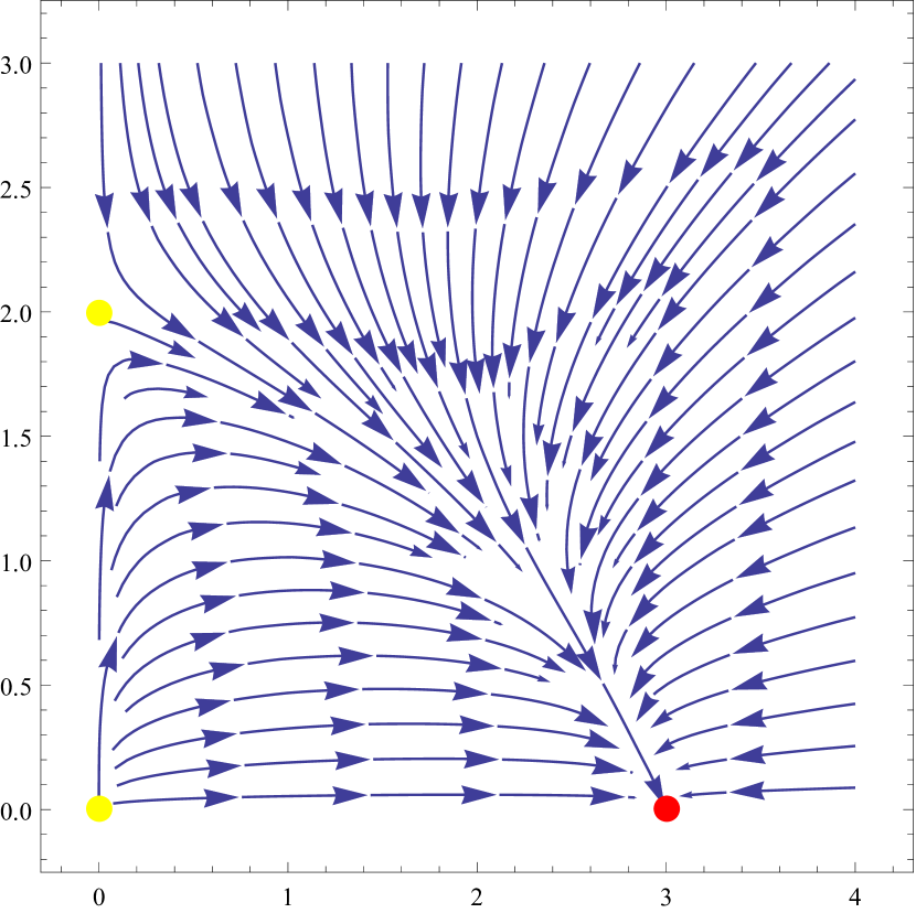
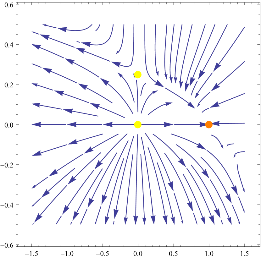
All results are listed in Table 2. To conclude this chapter, we have two different phase portraits of the dynamical system (1.1), shown in Figure 3.
2.1.3 Case and
Similarly as in the Section 2.1.2, from we conclude that the equilibrium coincides with and that . The equilibriums and are hyperbolic and their nature is the same as in Section 2.1.2 (Table 1), considering only the cases when . The equilibrium is nonhyperbolic (), and we will determine its stability by analyzing the phase trajectories around this equilibrium. However, we will only present the final results here, since the procedure is similar to the one presented in Section 2.1.2.
If , then equilibrium will be unstable (proof of this statement can be obtained using nullclines, similarly as in Section 2.1.2). If , then the equilibrium is semi-stable. The equilibrium is asymptotically stable on . To prove this statement, the reader can use the Lyapunov function . The equilibrium is unstable in . To prove this statement, the reader can use nullclines, similar to Section 2.1.2. The results are shown in the Table 3.
| eq. | and | and | |
|---|---|---|---|
| not possible case | U (u. node) | ||
| SS | |||
| U (saddle) | |||
| U (u. node) | not possible case | ||
| U | |||
| AS |
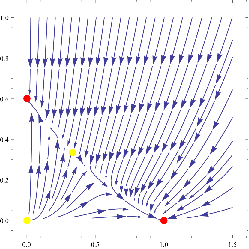
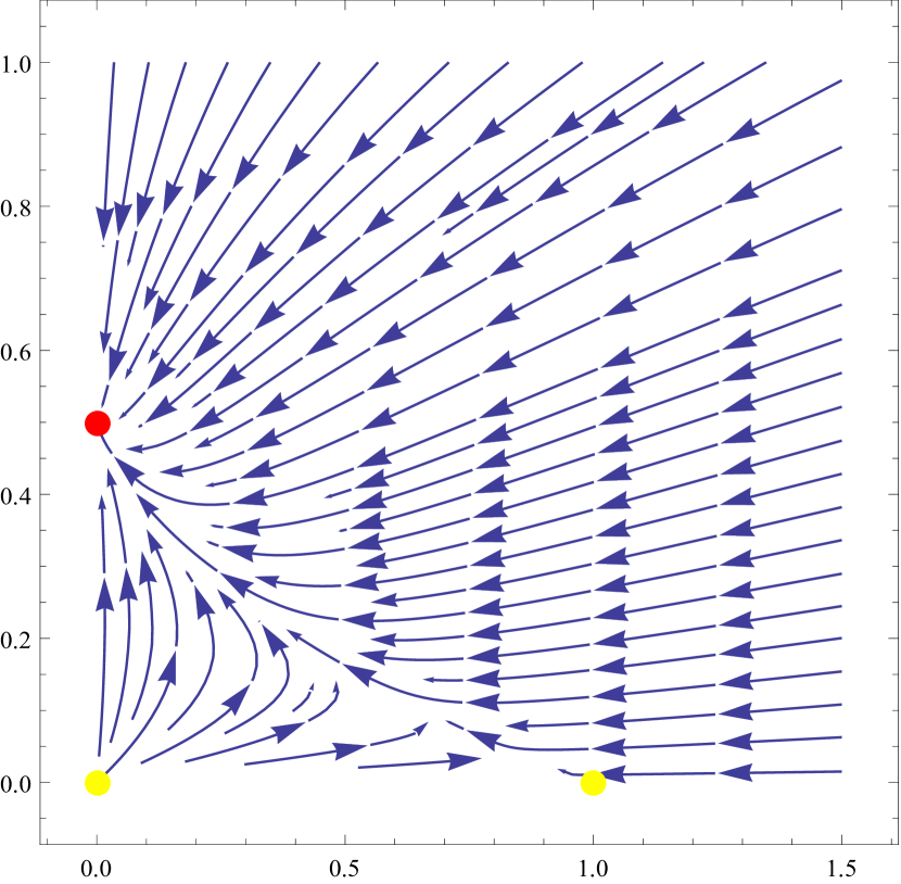
Therefore, in this section we have two different phase portraits of the dynamical system (1.1), which are shown in Figure 4.
2.1.4 Case and
This case is not possible. This can be shown in a similar way as in Section 2.1.2 (the proof differs if or ).
2.2 Case
We distinguish between two cases, when at least one minor is not equal to zero and when both minors are equal to zero.
2.2.1 Case or
The equilibrium does not exist in this case, since the system
| (2.6) |
has no solutions. Accordingly, the system (1.1) has three equilibriums, , and . If and , then all three equilibriums are hyperbolic and the conclusions regarding their stability are given in Table 4.
| eq. |
|
|
|
|
|---|---|---|---|---|
| U (u. node) | not possible cases | not possible cases | U (u. node) | |
| U (saddle) | AS (s. node) | |||
| AS (s. node) | U (saddle) |
Here the cases for and are impossible and the cases for , and are also impossible. The proofs are similar to those in Section 2.1.2 and so we omit them here.
We note that this section does not provide us with any qualitatively new phase portraits of the dynamical system (1.1), since we already had these qualitatively equal phase portraits before. For , , , we have the same phase portrait as for , , and , , from Section 2.1.1. Furthermore, for , , , we have the same phase portrait as for the , , and , , from Section 2.1.1.
2.2.2 Case and
If both minors are equal to zero, the system (2.6) has infinitely many solutions , where and . Consequently, the system (1.1) has infinitely many equilibriums, and , where . We note that the equilibriums are non-isolated and that for we conclude , while for we obtain . Therefore we exclude these values for in the following discussion.
The Jacobian matrix calculated for is given by
| (2.7) |
From (2.7), using and , we deduce that
| (2.8) |
from which we conclude that , , , since , and , . Thus, is nonhyperbolic equilibrium for every . is a nonhyperbolic equilibrium for every , i.e. is a line of equilibriums. is a hyperbolic equilibrium, which is an unstable node, just as in the previous sections. The phase portrait is shown in Figure 5.
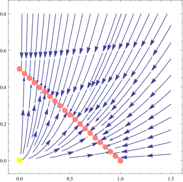
, .
The equilibrium at the origin is unstable, while the equilibriums , where , are non-isolated.
3 Necessary and sufficient conditions for stability of equilibriums
Section 2 shows that there are nine qualitatively different phase portraits of the dynamical system (1.1) which are shown in Figures 1-5, when we consider the stability of equilibriums of the system (1.1) on their full neighbourhoods. The signs of , and as well as the equilibriums of the dynamical system (1.1) are shown in Table 5.
| Serial No. | ||||||||
|---|---|---|---|---|---|---|---|---|
| 1 | U | U | U | AS | / | |||
| 2 | U | U | SS | / | / | |||
| 3 | U | U | AS | / | / | |||
| 4 | U | SS | U | / | / | |||
| 5 | U | AS | U | / | / | |||
| 6 | U | U | AS | / | / | |||
| 7 | U | AS | U | / | / | |||
| 8 | U | AS | AS | U | / | |||
| 9 | U | NI | NI | / | NI |
After analyzing Figures 1-5 and the data in Table 5, we conclude that the phase portraits under serial numbers 2, 3 and 6 that are shown in Figures 3(a), 1(b) and 4(b) have qualitatively the same dynamical properties in , i.e. that in the equilibrium is an unstable equilibrium and that the equilibrium is asymptotically stable.
Moreover, the phase portraits under serial numbers 4, 5 and 7 that are shown in Figures 4(a), 2(a) and 3(b) have qualitatively the same dynamical properties in , i.e. the equilibrium is asymptotically stable and the equilibrium is unstable.
In summary, we have nine qualitatively different phase portraits of the dynamical system (1.1) when we consider the stability of equilibriums of the system (1.1) on their full neighbourhoods, while we have five qualitatively different phase portraits when we analyze the stability of its equilibriums on . We note that it is interesting from mathematical point of view to analyze the stability of the equilibriums of the system (1.1) on their full neighbourhoods, although it lacks an appropriate physical interpretation since the density of the species cannot be negative.
To summarize all the results from the Section 2, we formulate the following theorems.
Theorem 3.1
The equilibrium of the system (1.1) is asymptotically stable on if and only if one of the following conditions is satisfied:
-
(1)
and (regardless of the );
-
(2)
and and ;
-
(3)
and and ;
-
(4)
and and .
Theorem 3.1 is an extension of Theorem 2.1. from [10] for , where it states (with a different notation than the one used here) that if and , then is asymptotically stable on .
Now we formulate a similar theorem for the equilibrium .
Theorem 3.2
The equilibrium of the system (1.1) is asymptotically stable on if and only if one of the following conditions is satisfied:
-
(1)
and (regardless of the );
-
(2)
and and ;
-
(3)
and and ;
-
(4)
and and .
As a consequence of Theorem 3.1 and Theorem 3.2 and the fact that is an unstable node (unstable equilibrium) regardless of the signs of , and , we formulate the following two theorems.
Theorem 3.3
Theorem 3.4
Moreover, the following can be concluded.
Theorem 3.5
Theorem 3.5 is an extension of Lemma 7.2. from [10] for , which states (with a different notation than the one used here) that if the system (1.1) satisfies the inequalities and , then there is no equilibrium in . The next theorem considers the stability of equilibrium .
Theorem 3.6
The equilibrium of the system (1.1) is:
-
(1)
asymptotically stable on if and only if and and ;
-
(2)
unstable if and only if and and .
4 Bifurcation analysis
As a consequence of Section 2, there are five different phase portraits of the system (1.1) in , which can be found in Table 5 under serial numbers 1, 2, 4, 8 and 9. They are already shown in Figures 1(a), 3(a), 4(a), 2(b) and 5 respectively. We note that it is interesting from mathematical point of view to analyze the stability of the equilibriums of the system (1.1) on , although it lacks an appropriate physical interpretation. In that case, four transcritical bifurcations can occur.
Comparing cases 1, 2 and 3 from Table 5 but with the stability of equilibriums analyzed on , we see that for (case 1) all equilibriums are hyperbolic and that , and are an unstable equilibriums, while is an asymptotically stable equilibrium. For (case 2), nonhyperbolic equilibrium collides with and becomes a semi-stable equilibrium, while the stability of other two equilibriums remains the same. Furthermore, for (case 3), the equilibrium appears again, but this time as an unstable equilibrium in the second quadrant, while the equilibrium is now an asymptotically stable equilibrium, i.e. the equilibrium have swapped stability with the equilibrium at , while the stability of other equilibriums have remained the same.
We notice similar situation when we compare cases 1, 4 and 5 from Table 5, again analyzing the system (1.1) on . More precisely, the equilibrium have swapped stability with (which transitioned from the first quadrant to the fourth quadrant) at . Furthermore, when we compare cases 8 and 6 from Table 5 and the case , and from Table 1 (again on ), we easily obtain that the equilibrium have swapped stability with the equilibrium (which transitioned from the first quadrant to the fourth quadrant) at if . Finally, when we compare cases 8 and 7 from Table 5 and the case , and from Table 1, we derive that the equilibrium have swapped stability with the equilibrium (which transitioned from the first quadrant to the second quadrant) at , again if .
5 Conclusion
We have analyzed the stability of equilibriums and bifurcations of the dynamical system (1.1) for various signs of the main and minor determinants of this system, , and . Of the total of twenty-seven different combinations of the signs of the determinants , and , thirteen were meaningful, while nine of them were different from each other on full neighbourhood of the equilibriums and their phase portraits are shown in Figures 1-5. Only five of these nine cases had different phase portraits on , which are shown in Figures 1(a), 3(a), 4(a), 2(b) and 5. Four of these five phase portraits can also be found in [7], while the last one is new and very specific as it has infinite equilibriums. All results are presented in Tables 1-5. In addition, we have improved several results from [10], mainly in terms of necessary and sufficient conditions for the equilibriums , and to be asymptotically stable or unstable. We noticed four transcritical bifurcations among thirteen meaningful and different phase portraits on .
References
- [1] S. Ahmad, On the nonautonomous Volterra-Lotka competition equations, Proc. Amer. Math. Soc., 117(1) (1993), 199–204.
- [2] S. Ahmad, A. C. Lazer, One species extinction in an autonomous competition model, Proceedings of the First World Congress of Nonlinear Analysis, Walter de Gruyter, Berlin, 1996, 359–368.
- [3] S. Ahmad, A. C. Lazer, Necessary and sufficient average growth in a Lotka–Volterra system, Nonlinear Anal., 34 (1998), 191–228.
- [4] E. Gonzalez-Olivares, A. Rojas-Palma, Stability in Kolmogorov-type quadratic systems describing interactions among two species. A brief revision, Selecciones Matemáticas, 8(1) (2021), 131–146.
- [5] J. Hofbauer, K. Sigmund, The theory of evolution and dynamical systems, Cambridge Univ. Press, Cambridge, 1988.
- [6] A. J. Lotka, Elements of Physical Biology, Williams-Wilkins, Baltimore, 1925.
- [7] F. Munteanu, A study of a three-dimensional competitive Lotka-Volterra system, ITM Web Conf., 34 (2020), 03010.
- [8] J. Murray, Mathematical Biology, Springer, New York, 1993.
- [9] V. Volterra, Leçon sur la Theorie Mathématique de la lutte pour la vie, Gauthier-Villars, Paris, 1931.
- [10] M. L. Zeeman, Extinction in competitive Lotka-Volterra systems, Proc. Amer. Math. Soc., 123(1) (1995), 87–96.
School of Electrical Engineering, University of Belgrade,
Bulevar kralja Aleksandra 73, 11120 Belgrade, Serbia
danijela@etf.bg.ac.rs
Faculty of Mathematics, University of Belgrade,
Studentski trg 16, 11158 Belgrade, Serbia
marija.mikic@matf.bg.ac.rs