ProFL: Performative Robust Optimal
Federated Learning

Abstract

Performative prediction (PP) is a framework that captures distribution shifts that occur during the training of machine learning models due to their deployment. As the trained model is used, its generated data could cause the model to evolve, leading to deviations from the original data distribution. The impact of such model-induced distribution shifts in the federated learning (FL) setup remains unexplored, despite being increasingly likely to transpire in real-life use cases. Although Jin et al., (2024) recently extended PP to FL in a straightforward manner, the resulting model only converges to a performative stable point, which may be far from optimal. The methods in Izzo et al., (2021); Miller et al., (2021) can find a performative optimal point in centralized settings, but they require the performative risk to be convex and the training data to be noiseless—assumptions often violated in realistic FL systems. This paper overcomes all of these shortcomings and proposes Performative robust optimal Federated Learning (ProFL), an algorithm that finds performative optimal points in FL from noisy and contaminated data. We present the convergence analysis under the Polyak-Lojasiewicz condition, which applies to non-convex objectives. Extensive experiments on multiple datasets validate our proposed algorithms’ efficiency.

Keywords Federated learning  $\cdot$ Performative prediction $\cdot$ Robust

1 Introduction

Federated learning (FL) is a distributed learning paradigm that enables efficient learning from heterogeneous clients. Conventional FL (e.g., collaborative model training) often relies on the unrealistic assumption that each client’s data distribution remains static throughout the training process or between the training and testing phases. Recent work addresses this weakness by training models on time-evolving data (Guo et al.,, 2023; Ma et al.,, 2022) or training models on static data but deploying them on different data distributions (Nguyen et al.,, 2022; Jiang and Lin,, 2022). However, these works assume that the changes in data distribution are exogenous (i.e., are independent of the FL system). Examples of such exogenous distribution shifts include variations in data quality, lighting conditions, dynamic climate data, etc.

In many real-world applications, data often undergoes performative endogenous shifts induced by the model’s deployment. For instance, content recommended by machine learning algorithms on digital platforms can reshape consumer preferences, steering them toward modes of consumption that are easier to predict and monetize (Dean and Morgenstern,, 2022). Similarly, navigation systems can influence traffic patterns, while individuals may adapt their behavior to game decision-making systems, such as those used for loan approvals or job applications (Hardt et al.,, 2016; Zhang et al.,, 2022). These types of shifts have been studied in centralized settings under the framework of performative prediction (PP), which seeks performative stable (Perdomo et al.,, 2020) or optimal (Izzo et al.,, 2021; Miller et al.,, 2021) solutions. Addressing endogenous shifts in federated learning (FL) is not a simple extension of these centralized efforts and remains a significant challenge. Failing to do so can lead to suboptimal performance or even non-convergence.

Another challenge in practical FL systems, beyond model-induced endogenous shifts, is data contamination. Client data may be noisy, corrupted, or maliciously manipulated. Unlike centralized systems, in FL, such data cannot be removed before training, as it remains with the clients. Developing FL systems that are robust to endogenous shifts and data contamination remains a significant challenge.

The only work to date that addresses the endogenous shifts in FL is Jin et al., (2024). Their approach assumes noiseless client data and only finds a performative stable point, which may be suboptimal. While Izzo et al., (2021); Miller et al., (2021) achieve a performative optimal point, their methods are centralized, assume noiseless data, and require convex performative risk. As we will show, the method that directly extends Izzo et al., (2021) to federated settings is highly vulnerable to data contamination and performs poorly when distribution shifts are complex.

In this paper, we solve all these challenges simultaneously and propose Performative robust optimal Federated Learning (ProFL), an FL algorithm that finds a performative optimal solution under endogenous distribution shifts with contaminated data. We provide a theoretical analysis of data contamination and the convergence of ProFL. Compared to the federated extension of Izzo et al., (2021), ProFL employs simple yet effective strategies and converges to the performative optimal solution for a larger class of (non-convex) objective functions. In Appendix B, we provide more related work and highlight differences.

Summary of contributions. Our key contributions compared to prior works are:

1. Finding the optimal solution. Unlike Jin et al., (2024), which only guarantees convergence to the stable point, ProFL finds the optimal point.

2. Convergence analysis for a larger class of objectives. Unlike prior works (Izzo et al.,, 2021; Jin et al.,, 2024) that show the convergence of the proposed algorithms for the convex performative risk, we show the convergence of ProFL under Polyak-Lojasiewicz (PL) condition, which is non-convex.

3. Robustness to data contamination. We analyze the impact of contaminated data on the FL system and show that ProFL effectively tackles complex distribution shifts and is more resilient to estimation error and data contamination.

2 Problem Formulation

Consider a set of clients $\mathcal{V}=\{1,\ldots,N\}$ collaboratively training an FL model $\theta\in\Theta\subset\mathbb{R}^{d}$ without sharing their local data. Here, $\Theta$ is a compact set (closed and bounded), and $d$ represents the model’s dimension. Let $\mathcal{Z}$ denote the sample space. Throughout training, each client interacts with the local model, causing its data to evolve based on the perceived model. Such model-induced data distributions, studied in PP (Perdomo et al.,, 2020), are characterized by a performative distribution map $D_{i}:\Theta\to\mathcal{P}(\mathcal{Z})$. Specifically, deploying model $\theta$ at client $i$ results in data following distribution $D_{i}(\theta)$. The goal is to train a global model that minimizes the total loss across all clients:

$${{\theta}}^{\text{PO}}=\mathop{\arg\min}\limits_{\theta}\mathcal{L}(\theta):=\sum_{i\in\mathcal{V}}\alpha_{i}\mathcal{L}_{i}(\theta)$$ (1)

where $\mathcal{L}_{i}(\theta)=\mathbb{E}_{Z_{i}\sim D_{i}(\theta)}[\ell(Z_{i};\theta)]$ is the local performative risk of client $i$ for a given loss function $\ell(Z_{i};\theta)$ on local data $Z_{i}\sim D_{i}(\theta)$. This is called performative risk because, instead of measuring the risk over a fixed distribution, it measures the expected loss of model $\theta$ on the data distribution $D_{i}(\theta)$ it induces. $\mathcal{L}(\theta)$ is the performative risk (PR) of all clients. Here, $\alpha_{i}\geq 0$ represents the fraction of client $i$’s data relative to the total, with $\sum_{i\in\mathcal{V}}\alpha_{i}=1$. The solution ${\theta}^{\text{PO}}$ that minimizes performative risk is called performative optimal (PO) point (Perdomo et al.,, 2020).

In realistic FL systems, each client’s data distribution $D_{i}(\theta)$ is unknown, and the training data may be noisy, corrupted, or maliciously manipulated. To account for this, we assume each client $i$ has a fraction $\epsilon_{i}\in[0,1]$ of data samples drawn from another fixed but arbitrary distribution $Q_{i}$. Thus, the data acquired from client $i$ follows a mixture distribution ${Z}_{i}\sim P_{i}(\theta)=(1-\epsilon_{i})D_{i}(\theta)+\epsilon_{i}Q_{i}$. We term $Q_{i}$ data “contamination”.

Our goal is to (i) design FL algorithms that converge to the performative optimal ${\theta}^{\text{PO}}$; (ii) study the impact of data contamination $Q_{i}$ and develop robust solutions. While data contamination has been studied in FL with static data, its effect in performative settings is unexplored. A moment’s thought reveals that when client data depends on the FL system, contamination in one client may cause a cascading effect across the network, making it crucial to investigate how this disrupts FL convergence. We will explore this in the paper. We next present the metrics in PP.

Performative stable point. Since the data distribution $D_{i}(\theta)$ depends on $\theta$, which is the variable being optimized, finding the performative optimal point is often challenging. Thus, existing works (Perdomo et al.,, 2020; Mendler-Dünner et al.,, 2020; Zhao,, 2022) have mostly focused on finding the so-called performative stable (PS) point. In an FL system, the PS point ${{\theta}}^{\text{PS}}$ is defined as follows:

$${{\theta}}^{\text{PS}}=\mathop{\arg\min}\limits_{\theta}\mathcal{L}({{\theta}}^{\text{PS}};\theta):=\sum_{i\in\mathcal{V}}\alpha_{i}\mathcal{L}_{i}({{\theta}}^{\text{PS}};\theta)$$ (2)

where $\mathcal{L}_{i}({{\theta}}^{{}^{\prime}};\theta)=\mathbb{E}_{Z_{i}\sim D_{i}({{\theta}}^{{}^{\prime}})}\left[\ell(Z_{i};\theta)\right]$ is called the decoupled performative risk (DPR) of client $i$. Unlike performative risk (PR), where the distribution $D_{i}(\theta)$ depends on $\theta$, the DPR decouples the two; i.e., the data distribution is induced by ${\theta}^{\text{PS}}$ while the variable being optimized is $\theta$. Since ${\theta}^{\text{PS}}$ is the fixed point of Eq. (2), it can be found via repeated risk minimization (RRM) or repeated gradient descent (RGD) (Perdomo et al.,, 2020). RRM recursively finds a model $\theta^{t+1}$ that minimizes DPR on the distribution $D(\theta^{t})$ induced by the previous model, whereas RGD recursively finds a model $\theta^{t+1}$ through gradient descent, and $\theta^{t+1}$ is not necessarily the minimizer of the DPR on $D(\theta^{t})$.

Following the idea of RGD, Jin et al., (2024) proposed the performative federated learning (PFL) algorithm to find the PS point ${\theta}^{\text{PS}}$ in FL. In PFL, each client $i$ updates its local model to reduce local DPR based on the previous model’s induced distribution: $\theta_{i}^{t+1}\leftarrow\theta_{i}^{t}-\eta_{t}\nabla\ell(Z_{i}^{t+1};\theta_{i}^{t})$, where $Z_{i}^{t+1}\sim D_{i}(\theta_{i}^{t})$ is drawn from the uncontaminated distribution. These updates are repeated for several epochs before being sent to the server for global aggregation. Jin et al., (2024) showed that PFL converges to ${\theta}^{\text{PS}}$ under clean data. Although the PS point is easier to find than the PO point, prior works (Izzo et al.,, 2021; Miller et al.,, 2021) show that the PS point may be far from optimal or may not even exist. Thus, algorithms like PFL, which target the PS point, are not ideal.

Performative gradient for performative optimal point. The key to finding the PO point is to update the model using the actual gradient of PR, $\nabla\mathcal{L}(\theta)$, also known as the performative gradient (PG). In FL, each client needs to update its model with its local PG: $\nabla\mathcal{L}_{i}(\theta)$. Assume $D_{i}(\theta)$ has density $p(z;f(\theta))$ with parameter $f(\theta)$ being a function of $\theta$, then $\mathcal{L}_{i}(\theta)=\int\ell(z;\theta)p(z;f_{i}(\theta))dz$ when $p$ and $f$ are continuously differentiable. PG can be derived

$$\nabla\mathcal{L}_{i}(\theta)=\nabla\mathcal{L}_{i,1}(\theta)+\nabla\mathcal{L}_{i,2}(\theta)$$ (3)

where

$$\nabla\mathcal{L}_{i,1}(\theta)=\mathbb{E}_{Z_{i}\sim D_{i}(\mathbf{\theta})}[\nabla\ell(Z_{i};\mathbf{\theta})]$$

and

$$\nabla\mathcal{L}_{i,2}(\theta)=\mathbb{E}_{Z_{i}\sim D_{i}(\theta)}\left[\ell(Z_{i};\theta)\left(\frac{df_{i}(\theta)}{d\theta}\right)^{T}\frac{\partial\log p\left(Z_{i};f_{i}(\theta)\right)}{\partial f_{i}(\theta)}\right].$$

Note that PFL proposed by Jin et al., (2024) only updates the model with $\nabla\mathcal{L}_{i,1}(\theta)$ while completely neglecting $\nabla\mathcal{L}_{i,2}(\theta)$. This error can accumulate, and eventually, PFL can converge to a PS point far from the optimal. Thus, computing the PG for a more accurate estimate is crucial, but estimating $\nabla\mathcal{L}_{i,2}(\theta)$ is challenging. Although Izzo et al., (2021) proposed a method to estimate the PG, its performance is only evaluated in a centralized setting under a specific performative distribution map $D_{i}(\theta)$ (i.e., when $f_{i}(\theta)$ is a linear function of $\theta$) without considering data contamination. Moreover, it assumes that PR is convex, which is often unrealistic.

In summary, an FL algorithm that yields the PO point, even under a clean distribution and with rather limiting assumptions, has not been developed previously. This paper fills that gap by proposing an FL algorithm that provably converges to the PO point, even with non-convex PR, and handles data contamination.

Remark 2.1.

FL finds the solution by alternating between global model aggregation at the central server and local model updates at the clients. In our proposed algorithms, we focus on the local updates, which work with different aggregation rules imposed by the server, such as differing weighted averages.

3 A Naive Extension from CS to FL

Consider first directly extending Izzo et al., (2021) to the FL setting. We shall call this naive algortihm Performative optimal Federated Learning (PoFL). The pseudocode is provided in Appendix A. In this algorithm, each active client $i$ in set $\mathcal{I}_{t}\subseteq\mathcal{V}$, after synchronization with the current global model $\overline{\theta}^{t}$, uses its local data to update the model from $\theta_{i}^{t}$ to $\theta_{i}^{t+R}$. During these updates, the data distribution changes, and consequently, client $i$ would use samples from the contaminated distribution $P_{i}(\theta_{i}^{t})$ to update $\theta_{i}^{t}$. To find the optimal ${\theta}^{\text{PO}}=\arg\min_{\theta}\sum_{i\in\mathcal{V}}\alpha_{i}\mathcal{L}_{i}(\theta)$, each client $i$ should estimate its local performative gradient $\nabla\mathcal{L}_{i}(\theta_{i}^{t})$ to update the local model $\theta_{i}^{t}$, i.e.,

$$\theta^{t+1}_{i}\leftarrow\text{Proj}_{\Theta}\left(\theta^{t}_{i}-\eta\nabla\mathcal{L}_{i}(\theta^{t}_{i})\right).$$ (4)

By Eq. (3), $\nabla\mathcal{L}_{i}(\theta_{i}^{t})=\nabla\mathcal{L}_{i,1}(\theta_{i}^{t})+\nabla\mathcal{L}_{i,2}(\theta_{i}^{t})$ consists of two terms. PoFL estimates $\nabla\mathcal{L}_{i,1}(\theta_{i}^{t})$ by simply averaging $\nabla\ell(z_{j};\theta_{i}^{t})$ over samples drawn from $P_{i}(\mathbf{\theta}_{i}^{t})$. We denote the empirical risk on data drawn from distribution $Q_{i}$ or $D_{i}(\mathbf{\theta}_{i}^{t})$ as $\widehat{\nabla}\mathcal{L}_{i,1}(Q_{i},\theta_{i}^{t})$ and $\widehat{\nabla}\mathcal{L}_{i,1}(D_{i}(\theta_{i}^{t}),\theta_{i}^{t})$, respectively. Then the empirical risk on $P_{i}(\mathbf{\theta}_{i}^{t})$ is $\widehat{\nabla}\mathcal{L}_{i,1}(\theta_{i}^{t}).$ Let $\widehat{\mathcal{L}}_{i,1}(\theta_{i}^{t})$ denotes the average of $\ell(z_{j};\theta_{i}^{t})$ over samples drawn from $P_{i}(\mathbf{\theta}_{i}^{t})$. We denote $\widehat{\nabla}\mathcal{L}_{i,2}(\theta_{i}^{t})$, $\widehat{\nabla}\mathcal{L}_{i,2}(Q_{i},\theta_{i}^{t})$, and $\widehat{\nabla}\mathcal{L}_{i,2}(D_{i}(\theta_{i}^{t}),\theta_{i}^{t})$ similarly. $\widehat{\nabla}\mathcal{L}_{i,2}(\theta_{i}^{t})$ is estimated by a weighted average of $\ell(z_{j};\theta_{i}^{t})$ over samples drawn from $P_{i}(\mathbf{\theta}_{i}^{t})$ with weight vector

$$w(z_{j};\theta_{i}^{t}):=\left.\left(\frac{df_{i}(\theta)}{d\theta}\right)^{T}\frac{\partial\log p(z_{j};f_{i}(\theta))}{\partial f_{i}(\theta)}\right|_{\theta=\mathbf{\theta}_{i}^{t}}\in\mathbb{R}^{d}$$ (5)

Because the distribution map $D_{i}(\theta)=p(z;f_{i}(\theta))$ and $f_{i}(\theta)$ are unknown, we need to estimate $f_{i}(\theta)$ and $\frac{df_{i}(\theta)}{d\theta}.$ Following Izzo et al., (2021), we adopt finite difference approximation $\left.\frac{df_{i}(\theta)}{d\theta}\right|_{\theta=\theta^{t}_{i}}\approx\Delta f_{i}(\Delta\theta_{i})^{\dagger}$. Specifically, at iteration $t$, each client $i$ collects the $H$ most recent models (excluding $\theta^{t}_{i}$) and forms a matrix $\begin{bmatrix}\theta^{t-H}_{i}&\cdots&\theta^{t-1}_{i}\end{bmatrix}$, then

$$\Delta\theta_{i} =\begin{bmatrix}\theta^{t-H}_{i}&\cdots&\theta^{t-1}_{i}\end{bmatrix}-\theta^{t}_{i}\textbf{1}^{T}_{H};$$ (6)

$$\Delta f_{i} =\begin{bmatrix}f_{i}(\theta^{t-H}_{i})&\cdots&f_{i}(\theta^{t-1}_{i})\end{bmatrix}-f_{i}(\theta^{t}_{i})\textbf{1}^{T}_{H},$$

Where $\textbf{1}_{H}$ is an $H$-dimensional all-ones vector, both $\Delta f_{i}$ and $\Delta\theta_{i}$ are $d\times H$ matrices, and $(\Delta\theta_{i})^{\dagger}$ is the pseudo-inverse of $\Delta\theta_{i}$. For each iteration of each client, we know $\theta_{i}^{t}$, but do not know the exact value of $f_{i}(\theta_{i}^{t})$. Denote the estimator as $\widehat{f}_{i}(\mathcal{S}_{i})$, meaning we use the dataset $\mathcal{S}_{i}$ and the function $\widehat{f}_{i}(.)$ to estimate the value of $f_{i}(\theta_{i}^{t})$. This estimator is then used to compute an estimate of $\frac{df_{i}}{d\theta}$. The estimator of $\frac{df_{i}}{d\theta}$ is denoted as $\frac{\widehat{df_{i}}}{d\theta}$ and can be computed as $\frac{\widehat{df_{i}}}{d\theta}\approx\widehat{f}_{i}(\Delta\theta_{i})^{\dagger}$. Finally, $\frac{\widehat{df_{i}}}{d\theta}$ will be used to calculate $\widehat{\nabla}\mathcal{L}_{i,2}$. By combining this with $\widehat{\nabla}\mathcal{L}_{i,1}$, we obtain the performative gradient, allowing each client to update the local model $\theta_{i}^{t}$ using Eq. (4).

Concerns with POFL. Although Izzo et al., (2021) showed that the above method for estimating $f_{i}(\theta)$ and $\frac{df_{i}(\theta)}{d\theta}$ was effective in centralized settings, it was evaluated under specific scenarios where $f_{i}(\theta)$ is linear in $\theta$ and data samples perfectly represent $D_{i}(\theta)$ without contamination. In practical FL settings with model-induced distribution shift, this method will perform poorly due to the following reasons:

1. Non-linearity of $f_{i}(\theta)$. When $f_{i}(\theta)$ is non-linear, ignoring the higher-order terms in the Taylor expansion of $\frac{\widehat{df_{i}}}{d\theta}$ may be biased. While Izzo et al., (2021) demonstrated that this method works well for linear $f_{i}(\theta)$, the impact of non-linearity on performance remains unclear.

2. Amplified sampling error. Since $\frac{df_{i}(\theta)}{d\theta}$ is estimated from limited samples, the sampling error of the estimation $\Delta f_{i}(\Delta\theta_{i})^{\dagger}$ is inherited when computing PG, $\nabla\mathcal{L}_{i}(\theta_{i}^{t})$. As shown in Lemmas 5.7, 5.8 and  5.9 in Section 5, the sampling error in estimating $\frac{df_{i}(\theta)}{d\theta}$ is amplified when computing $\nabla\mathcal{L}_{i,2}(\theta_{i}^{t})$, making the performative gradient and algorithm more sensitive to sampling errors.

3. Contaminated data. Due to contamination $Q_{i}$, the data used for estimating $\frac{df(\theta)}{d\theta}$ and $f_{i}(\theta)$ does not follow the actual $D_{i}(\theta)$. Even a small error in a single model update for one client can cascade, affecting subsequent data and the entire network.

4 The Proposed Algorithm: PROFL

The previous section summarized the drawbacks of a straightforward extension of the centralized solution to the federated setting. To address all these weaknesses, we propose several simple yet effective strategies that lead to a robust new FL algorithm. We shall call it Performative robust optimal Federated Learning (ProFL). The pseudocode is provided in Algorithm 1. Below are its key features.

Algorithm 1 ProFL

1:  Input: Learning rate $\eta$, estimation window $H$, function $\widehat{f}$, total iterations $T$, local update iterations $R$, error bound $\Phi_{i}$ for all $i\in\mathcal{V}$.

2:  for $t=0$ to $T-1$ do

3:     If $t\mod R=0$, server sends $\overline{\theta}^{t}$ to a selected set $\mathcal{I}_{t}\subseteq\mathcal{V}$ of clients and client $i\in\mathcal{I}_{t}$ sets the local model $\theta^{t}_{i}=\overline{\theta}^{t}$; otherwise $\mathcal{I}_{t}=\mathcal{I}_{t-1}.$

4:     for $i\in\mathcal{I}_{t}$ in parallel do

5:        Deploy $\theta^{t}_{i}$ and local environment changes and draw $n_{i}$ samples $\mathcal{S}_{i}:=(z_{j})^{n_{i}}_{j=1}\mathop{\sim}\limits^{iid}P_{i}(\theta^{t}_{i})$.

6:        if $t\leq H$ then

7:           $\widehat{\nabla}\mathcal{L}_{i,1}(\theta^{t}_{i});\mathcal{S}^{\prime}_{i}\leftarrow\textsc{Robust Gradient}\left(\mathcal{S}_{i};\theta^{t}_{i}\right).$

8:           Compute estimator $\widehat{f}\left(\mathcal{S^{\prime}}_{i}\right)$ of $f^{t}_{i}$.

9:           Update $\theta^{t+1}_{i}\leftarrow\text{Proj}_{\Theta}\left(\theta^{t}_{i}-\eta\widehat{\nabla}\mathcal{L}_{i,1}(\theta^{t}_{i})\right)$

10:        else

11:           $\widehat{\mathcal{L}}_{i,1}(\theta^{t}_{i});\widehat{\nabla}\mathcal{L}_{i,1}(\theta^{t}_{i});\mathcal{S}^{\prime}_{i}\leftarrow\textsc{Robust Gradient}\left(\mathcal{S}_{i};\theta^{t}_{i}\right)$

12:           Compute estimator $\widehat{f}\left(\mathcal{S^{\prime}}_{i}\right)$ of $f^{t}_{i}$.

13:           Form matrices $\Delta\theta_{i}$ and $\Delta f_{i}$ and compute $\Delta f_{i}(\Delta\theta_{i})^{\dagger}$.

14:           $\theta^{t+1}_{i}\leftarrow\text{Proj}_{\Theta}\left(\theta^{t}_{i}-\eta\left(\widehat{\nabla}\mathcal{L}_{i,1}(\theta^{t}_{i})+\widehat{\nabla}\mathcal{L}_{i,2}(\theta^{t}_{i})\right)\right)$.

15:           Input$=\{\widehat{\mathcal{L}}_{i,1}(\theta^{t}_{i});H;d;\eta;\varphi_{i};\Delta f_{i}(\Delta\theta_{i})^{\dagger};\Phi_{i}\}$

16:           $n_{i}\leftarrow\textsc{Adaptive Sample Size}\left(\texttt{Input}\right)$.

17:     If $t\mod R=0$, client $i\in\mathcal{I}_{t}$ sends $\theta^{t}_{i}$ to the server and server updates the model $\overline{\theta}^{t+1}=\sum_{i\in\mathcal{I}_{t}}\alpha_{i}\theta^{t+1}_{i}$.

18:  Output: $\overline{\theta}^{T}$

1. Handling complex distribution shifts with non-linear $f_{i}(\theta)$. ProFL employs the following strategies: (i) reducing the learning rate $\eta$ and the estimation window $H$; (ii) estimating $\widehat{\frac{df_{i}}{d\theta}}$ at the server. Reducing $\eta$ and $H$ helps reduce the estimation error resulting from non-linear $f_{i}(\theta)$ and stabilizes the algorithm. When the local sample size $n_{i}$ is small, $\widehat{f}_{i}(\mathcal{S}_{i})$ may significantly deviate from $f_{i}(\theta)$, leading to poor estimation of $\frac{df_{i}}{d\theta}$. Estimating $\widehat{\frac{df_{i}}{d\theta}}$ at the server mitigates the negative impact of sampling error.

2. Balancing the impact of sampling error and computational costs. ProFL adaptively selects the sample size $n_{i}$ based on the error bounds of the PG and local loss. While a larger $n_{i}$ generally leads to a more accurate estimate, it may not always be feasible in FL due to clients’ limited computational capabilities. By using predefined error bounds and relevant computed values—such as model variance, loss function, gradient information, and learning rates—we can determine the lower bound for each client’s $n_{i}$, balancing sampling error and computational costs. As these values change during updates, $n_{i}$ should be selected adaptively. More details are provided in Section 5.3.

3. Handling data contamination. ProFL mitigates contamination $Q_{i}$ by reducing $\epsilon_{i}$ through local outlier identification and removal. Since the samples $\mathcal{S}_{i}\sim P_{i}(\theta_{i}^{t})$are noisy, and the raw data is not visible to the central server, contamination must be identified and cleaned locally before estimating the performative gradient $\nabla\mathcal{L}_{i}=\nabla\mathcal{L}_{i,1}+\nabla\mathcal{L}_{i,2}$. Given the contaminated dataset $\mathcal{S}_{i}$, each client in ProFL uses algorithm Robust gradient to identify “clean” samples $\mathcal{S}^{\prime}_{i}=\{z_{j}\in\mathcal{S}_{i}:z_{j}\sim D_{i}(\theta_{i}^{t})\}$ and compute robust gradient $\nabla\mathcal{L}_{i,1}(\theta_{i}^{t})$. $\mathcal{S}^{\prime}_{i}$ are then used to estimate $\nabla\mathcal{L}_{i,2}(\theta_{i}^{t})$. The outlier identification and removal mechanism reduces $\epsilon_{i}$ (the fraction of contaminated data) and can be selected based on prior knowledge of $\epsilon_{i},Q_{i}$ (if there are any). In Appendix A, we provide an example of Robust Gradient for a general case with unknown $\epsilon_{i}$ and arbitrary $Q_{i}$. It uses singular value decomposition (SVD) to detect gradients that meet two key properties: 1) having a significant impact on the model and potentially disrupting training (i.e., gradients with large magnitudes that systematically point in a specific direction); and 2) being far from the average in the vector space (i.e., “long tail” data). We iteratively remove gradients whose distance from the average exceeds a threshold. More details on the Robust Gradient mechanism and its comparison to prior work are provided in Appendix  A.

In section 5, we analyze both algorithms’ convergence and the impact of the factors above on performance. Compared to PFL Jin et al., (2024) and methods in Izzo et al., (2021); Miller et al., (2021), we relax assumptions and show convergence under weaker conditions.

5 Performance Analysis

To facilitate analysis, we consider scenarios where $D_{i}(\theta)=\sum_{k=1}^{K}\nu_{i,k}(\theta)D_{i,k}(\theta)$ represents a mixture of $K$ group distributions. $\nu_{i,k}(\theta)$ is the proportion of samples from group $k$ and $\sum_{k=1}^{K}\nu_{i,k}(\theta)=1$. Let $f_{i,k}(.)$ denote the function for each group’s distribution.

We study two special cases: (i) Contribution dynamics, where only $\nu_{i,k}(\theta)$ changes while the group distribution remains fixed, i.e., $D_{i}(\theta)=\sum_{k\in[K]}\nu_{i,k}(\theta)D_{i,k}$. In this case, $f_{i,k}(\theta)=\nu_{i,k}(\theta)$, and $\widehat{f}_{i,k}$ estimates the sample proportion from group $k$. (ii) Distribution dynamics, where only the distribution $D_{i,k}(\theta)$ changes while the contribution from each group remains fixed, i.e., $D_{i}(\theta)=\sum_{k\in[K]}\nu_{i,k}D_{i,k}(\theta)$. We consider a mixture of Gaussians with $D_{i,k}(\theta)=\mathcal{N}(f_{k}(\theta),\sigma_{k}^{2})$, where $f_{i,k}(\theta)$ is the mean of group $k$ for client $i$, and the overall mean for client $i$ is $f_{i}(\theta)=\sum_{k\in[K]}\nu_{i,k}f_{i,k}(\theta)$. $\widehat{f}_{i}(\mathcal{S}_{i})$ represents the empirical mean from data samples $\mathcal{S}_{i}$. Our theoretical results apply to both cases. Before presenting them, we introduce the technical assumptions. For simplicity, $\|.\|_{2}$ is denoted as $\|.\|$. Proofs are in Appendix C.

Assumption 5.1.

Let $W_{1}(D,D^{\prime})$ measure the Wasserstein-1 distance between two distributions $D$ and $D^{\prime}$. Then $\forall i\in\mathcal{V}$, there exists $\gamma_{i}>0$ such that $\forall\theta,\theta^{\prime}\in\Theta:W_{1}\left(D_{i}(\theta),D_{i}(\theta^{\prime})\right)\leq\gamma_{i}{\|\theta-\theta^{\prime}\|}.$

Assumption 5.2.

$\ell(z;\mathbf{\theta})$ is continuously differentiable and $L$-smooth, i.e., for all $\theta\in\Theta\text{ and }z,z^{\prime}\in\mathcal{Z}:\|\nabla\ell(z;\mathbf{\theta})-\nabla\ell(z^{\prime};\mathbf{\theta^{\prime}})\|\leq L(\|\mathbf{\theta}-\mathbf{\theta^{\prime}}\|+\|z-z^{\prime}\|).$

Assumption 5.3.

$f_{i}(\theta)$ is twice continuously differentiable for all $\theta\in\Theta,$ i.e., the first and second derivatives $\frac{df_{i}(\theta)}{d\theta}$ and $\frac{d^{2}f_{i}(\theta)}{d\theta^{2}}$ exist and are continuous.

Assumption 5.4 (PL Condition Polyak, (1964)).

The local performative risk $\mathcal{L}_{i}(\theta)$ of client $i$ satisfies Polyak- Lojasiewicz (PL) condition, i.e., for all $\theta\in\Theta$, the following holds for some $\rho>0$:

$$\frac{1}{2}\|\nabla\mathcal{L}_{i}(\theta)\|^{2}\geq\rho\left(\mathcal{L}_{i}(\theta)-\mathcal{L}_{i}(\theta_{i}^{\text{PO}})\right).$$

Remark 5.5.

Unlike most works that require convex performative risk, we demonstrate the convergence of our algorithm under a weaker PL condition, which permits the performative risk to be non-convex.

5.1 Error of the performative gradient

As discussed in Section 3, the key to converging to $\theta^{\text{PO}}$ is estimating the performative gradient $\nabla\mathcal{L}_{i}(\theta_{i}^{t})=\nabla\mathcal{L}_{i,1}(\theta_{i}^{t})+\nabla\mathcal{L}_{i,2}(\theta_{i}^{t})$ in Eq. (3) accurately. Thus, we analyze the estimation errors of $\nabla\mathcal{L}_{i,1}(\theta_{i}^{t})$ and $\nabla\mathcal{L}_{i,2}(\theta_{i}^{t})$ and explore how these errors are influenced by the non-linearity of $f_{i}(\theta)$, sampling error, and contaminated data $Q_{i}$. The results of this analysis will then be used to assess the convergence of ProFL (and PoFL) in Section 5.2.

Lemma 5.6.

Under Assumption 5.3, there exist $F,M<\infty$ such that $\left\|\frac{df_{i}(\theta)}{d\theta}\right\|\leq F$ and $\left\|\frac{d^{2}f_{i}(\theta)}{d\theta^{2}}\right\|\leq M$ hold for all $i\in\mathcal{V}.$ Under Assumption 5.2, there exist $G,\ell_{\max}<\infty$ such that $\|\nabla\ell(z;\mathbf{\theta})\|\leq G$ and $\ell(z;\mathbf{\theta})\leq\ell_{\max}$ hold for all $z\in\mathcal{Z}$.

Lemma 5.6 is proved using Weierstrass’s theorem. We will use $F,M,G,\ell_{\max}$ to denote the upper bounds of these quantities in the rest of the paper.

Lemma 5.7 (Estimation error of $\frac{\widehat{df_{i}}}{d\theta}$).

Under Assumption 5.3, let $\lambda_{i,\min}$ denote the minimal singular value of $\Delta\theta_{i}$ defined in Eq. (6) during all iterations. With probability at least $1-\varphi_{i}$, the estimation error of $\frac{\widehat{df_{i}}}{d\theta}$ is bounded by $\boldsymbol{\omega_{F}}$ specified as follows:

$$\mathbb{E}\left[\left\|\frac{\widehat{df_{i}}}{d\theta}-\frac{df_{i}}{d\theta}\right\|^{2}\right]\leq\boldsymbol{\omega_{F}}:=2\epsilon_{i}^{2}F^{2}+(1-\epsilon_{i})^{2}\left(\frac{M^{2}\eta^{4}G^{4}H^{6}}{2}+\frac{2f_{\varphi}(\varphi_{i};n_{i})Hd}{n_{i}\eta^{2}}\right)\lambda^{-2}_{i,\min}.$$ (7)

Notably, $f_{\varphi}(\varphi_{i};n_{i})$ is a function that depends on the properties of the distribution. For instance, $f_{\varphi}(\varphi_{i};n_{i})=\mathcal{O}(-\log\varphi_{i})$ in distribution dynamics, and $f_{\varphi}(\varphi_{i};n_{i})=\mathcal{O}(1/\varphi_{i})$ in contribution dynamics.

Lemma 5.8 (Estimation error of $\nabla\mathcal{L}_{i,1}$).

Under Assumption 5.3, with probability at least $1-\varphi_{i}$, we have:

$$\mathbb{E}\left[\left\|\nabla\mathcal{L}_{i,1}(\theta_{i}^{t})-\widehat{\nabla}\mathcal{L}_{i,1}(D_{i}(\theta_{i}^{t}),\theta_{i}^{t})\right\|^{2}\right]\leq\mathcal{O}\left(f_{\varphi}(\varphi_{i};n_{i})\right).$$

Lemma 5.9 (Estimation error of $\nabla\mathcal{L}_{i,2}$).

Under Assumptions 5.1, 5.2 and 5.3, the following holds with probability at least $1-\varphi_{i}$:

$$\mathbb{E}\left[\left\|\nabla\mathcal{L}_{i,2}(\theta_{i}^{t})-\widehat{\nabla}\mathcal{L}_{{i,2}}(D_{i}(\theta_{i}^{t}),\theta_{i}^{t})\right\|^{2}\right]\leq(\boldsymbol{\omega_{D}})^{2}:=\mathcal{O}\left(\ell^{2}_{\max}d\left(\boldsymbol{\omega_{F}}+\frac{f_{\varphi}(\varphi_{i};n_{i})F^{2}}{n_{i}}\right)\right).$$

$$\mathbb{E}\left[\left\|{\nabla}\mathcal{L}_{{i,2}}(Q_{i},\theta_{i}^{t})-\widehat{\nabla}\mathcal{L}_{{i,2}}(Q_{i},\theta_{i}^{t})\right\|^{2}\right]\leq(\boldsymbol{\omega_{Q}})^{2}:=\mathcal{O}\left(2\ell^{2}_{\max}d\left(\boldsymbol{\omega_{F}}+F^{2}\right)\right).$$

Additionally, the notations $\boldsymbol{\omega_{D}}$ and $\boldsymbol{\omega_{Q}}$ represent upper bounds. From Lemmas 5.8 and 5.9, we find that since the estimation error of performative gradient is primarily dominated by the estimation error of $\nabla\mathcal{L}_{i,2}$, we have:

$$\mathbb{E}\left[\left\|\nabla\mathcal{L}_{i,1}(\theta_{i}^{t})-\widehat{\nabla}\mathcal{L}_{i,1}(D_{i}(\theta_{i}^{t}),\theta_{i}^{t})\right\|^{2}\right]+\mathbb{E}\left[\left\|\nabla\mathcal{L}_{i,2}(\theta_{i}^{t})-\widehat{\nabla}\mathcal{L}_{{i,2}}(D_{i}(\theta_{i}^{t}),\theta_{i}^{t})\right\|^{2}\right]\leq(\boldsymbol{\omega_{D}})^{2}.$$ (8)

5.2 Convergence analysis

Given Lemmas 5.7, 5.8, and 5.9, we are now ready to analyze the convergence. Denote $\overline{\gamma}=\sum_{i\in\mathcal{V}}\alpha_{i}\gamma_{i}$, $\sigma^{2}_{\gamma}=\sum_{i\in\mathcal{V}}\alpha_{i}(\overline{\gamma}-\gamma_{i})^{2}$, $\overline{\epsilon}=\sum_{i\in\mathcal{V}}\alpha_{i}\epsilon_{i}$, and $\varphi=\sum_{i\in\mathcal{V}}\varphi_{i}.$ Throughout the training process, let $W_{1}(D,Q)_{\max}$ represent the maximum Wasserstein-1 distance $W_{1}\left(D(\theta_{i}^{t}),Q_{i}\right)$ between actual data distribution and contamination $\forall i\in\mathcal{V}$. Let $\overline{\boldsymbol{\omega_{Q}}},\overline{\boldsymbol{\omega_{D}}}$ be the maximum of $\boldsymbol{\omega_{Q}}$ and $\boldsymbol{\omega_{D}}$ respectively in Lemma 5.9 $\forall i\in\mathcal{V}$. Let $g^{2}_{\min}$ be the minimal value of $\mathbb{E}[\|g^{t}\|^{2}]$ with $g^{t}=\sum_{i\in\mathcal{V}}\alpha_{i}\sum_{k=1}^{K}\widehat{\nabla}\mathcal{L}_{{i,k}}.$

Theorem 5.10 (Convergence rate).

Let $\{\overline{\theta}^{t}\}_{t\geq 0}$ be a sequence of global models generated by ProFL (and PoFL). Under Assumptions 5.1, 5.2, 5.3, and 5.4, with probability at least $1-T\varphi$, we have:

$$\mathbb{E}\left[\mathcal{L}\left(\overline{\theta}^{T}\right)-\mathcal{L}\left({\theta}^{\text{PO}}\right)\right]\leq \left(1-\rho\eta\right)^{T}\mathbb{E}\left[\mathcal{L}\left(\overline{\theta}^{0}\right)-\mathcal{L}\left({\theta}^{\text{PO}}\right)\right]+\left((1-\overline{\epsilon})\overline{\boldsymbol{\omega_{D}}}^{2}+\overline{\epsilon}\left(\overline{\boldsymbol{\omega_{D,Q}}}\right)^{2}-\frac{g^{2}_{\min}}{2}\right)\eta$$

$$\quad+\left(L(1+\overline{\gamma})\left((1-\overline{\epsilon})\overline{\boldsymbol{\omega_{D}}}^{2}+\overline{\epsilon}\left(\overline{\boldsymbol{\omega_{D,Q}}}\right)^{2}+G^{2}\right)\right)\eta^{2}$$

$$\quad+\frac{1}{2}L^{2}(R-1)^{2}G^{2}\left((1+\overline{\gamma})^{2}+\sigma^{2}_{\gamma}\right)\eta^{3}.$$

where $\overline{\boldsymbol{\omega_{D,Q}}}=\overline{\boldsymbol{\omega_{D}}}+LW_{1}(D,Q)_{\max}+\overline{\boldsymbol{\omega_{Q}}}.$

Theorem 5.10, together with Lemmas 5.7, 5.8 and 5.9 in Section 5.1, highlight the impact of sampling error, data contamination, client heterogeneity, and the non-linearity of $f_{i}(\theta)$ on convergence, as discussed below.

When there is no data contamination and $\epsilon_{i}=0$, $\boldsymbol{\omega_{F}}$ is reduced to $\left(\frac{M^{2}\eta^{2}G^{4}H^{6}}{2}+\frac{2f_{\varphi}(\varphi_{i};n_{i})Hd}{n_{i}\eta^{2}}\right)\lambda_{i,\min}^{-2}$, where the first term is due to the non-linearity of $f_{i}(\theta)$ and becomes zero if $f_{i}(\theta)$ is linear with $M=0$; the second term, related to sampling error, approaches zero as the sample size $n_{i}\to\infty$. With sufficient samples, the error term $\frac{f_{\varphi}(\varphi_{i};n_{i})F^{2}}{n_{i}}$ in $\boldsymbol{\omega_{D}}$ also approaches zero.

When there is contamination or $f_{i}(\theta)$ is non-linear, the error always exists even with a sufficiently large sample size. The term $\overline{\epsilon}(\overline{\boldsymbol{\omega_{D}}}+LW_{1}(D,Q)_{\max}+\overline{\boldsymbol{\omega_{Q}}})^{2}$ reflects the impact of contaminated data, increasing as the fraction of contamination $\epsilon_{i}$ and/or the distance between actual data distribution $D_{i}(\theta)$ and contamination $Q_{i}$ increase.

The term $L^{2}(R-1)^{2}G^{2}\eta\left((1+\overline{\gamma})^{2}+\sigma^{2}_{\gamma}\right)$ captures the effect of client heterogeneity. Recall that $R$ is the number of local updates. In the special case where $R=1$ , meaning clients update and aggregate models at each iteration, this term becomes zero.

Corollary 5.11.

If $\overline{\epsilon}=0$ (without contamination), the bound in Theorem 5.10 is reduced to the following:

$$\mathbb{E}\left[\mathcal{L}(\overline{\theta}^{T})-\mathcal{L}({\theta}^{\text{PO}})\right]\leq (1-\rho\eta)^{T}\mathbb{E}\left[\mathcal{L}(\overline{\theta}^{0})-\mathcal{L}({\theta}^{\text{PO}})\right]+\left(\overline{\boldsymbol{\omega_{D}}}^{2}-\frac{g^{2}_{\min}}{2}\right)\eta+L(1+\overline{\gamma})\left(\overline{\boldsymbol{\omega_{D}}}^{2}+G^{2}\right)\eta^{2}$$

$$\quad+\left(\frac{1}{2}L^{2}(R-1)^{2}G^{2}\left((1+\overline{\gamma})^{2}+\sigma^{2}_{\gamma}\right)\right)\eta^{3}.$$

Because $g^{2}_{\min}\geq 0,$ we consider two cases:

1. If $g^{2}_{\min}>0$, we can always adjust learning rate $\eta$, estimation window $H$, number of local updates $R$, and sample size $n_{i}$ such that $\overline{\boldsymbol{\omega_{D}}}^{2}<g^{2}_{\min}/2$ and the following holds

   $$\mathbb{E}\left[\mathcal{L}(\overline{\theta}^{T})-\mathcal{L}(\overline{\theta}^{\text{PO}})\right]\leq(1-\rho\eta)^{T}\mathbb{E}\left[\mathcal{L}(\overline{\theta}^{0})-\mathcal{L}({\theta}^{\text{PO}})\right],$$

   i.e., $\overline{\theta}^{t}$ converges to ${\theta}^{\text{PO}}$ at linear convergence rate.

2. If $g^{2}_{\min}=0$, this means there is at least one iteration $t$ that has $\|g^{t}\|=0$ and $\mathbb{E}[\mathcal{L}(\overline{\theta}^{t+1})-\mathcal{L}({\theta}^{\text{PO}})]=\mathbb{E}[\mathcal{L}(\overline{\theta}^{t})-\mathcal{L}({\theta}^{\text{PO}})]$. Except for the iterations where $\|g^{t}\|=0$, all the other iterations have positive $\|g^{t}\|>0$. We can choose $\eta,H,n_{i}$ such that $\overline{\boldsymbol{\omega_{D}}}^{2}<g^{2}_{\min}/2$ and the following holds

   $$\mathbb{E}\left[\mathcal{L}(\overline{\theta}^{T})-\mathcal{L}({\theta}^{\text{PO}})\right]\leq(1-\rho\eta)^{T-b}\mathbb{E}\left[\mathcal{L}(\overline{\theta}^{0})-\mathcal{L}({\theta}^{\text{PO}})\right],$$

   where $b$ is the number of iterations with $\|g^{t}\|=0$.

All above theoretical results apply to both ProFL and PoFL. The robust strategies in ProFL reduce the upper bound in Theorem 5.10.

5.3 Discussion

Section 3 introduced simple yet effective strategies in ProFL to enhance PoFL. We now explain why these strategies are effective.

Handling complex distribution shifts with non-linear $f_{i}(\theta)$. Based on Lemma 5.7, the non-linear function $f_{i}(\theta)$ primarily impacts the estimation error through the term $\frac{M^{2}\eta^{2}G^{4}H^{6}}{2}$, which decreases as $\eta$ and$H$ are reduced. However, to ensure the matrix $\Delta\theta_{i}$ in Eq. (6) is nonsingular, $H-1$ must be larger than the dimensionality of $\theta$. In cases where $H$ cannot be decreased, reducing $\eta$ is essential to attain a smaller $\boldsymbol{\omega_{F}}$. Moreover, the upper bound in Theorem 5.10 takes the form $A\eta+B\eta^{2}+C\eta^{3}$, where $B,C,\eta>0$. Thus, a smaller $\eta$ results in a smaller upper bound. However, reducing $\eta$ will also increase the error term $\frac{2f_{\varphi}(\varphi_{i};n_{i})Hd}{n_{i}\eta^{2}}$ in Eq. (7). Nevertheless, if the sample size $n_{i}$ is sufficiently large and $\frac{M^{2}\eta^{2}G^{4}H^{6}}{2}\gg\frac{2f_{\varphi}(\varphi_{i};n_{i})Hd}{n_{i}\eta^{2}}$, reducing the learning rate is still effective, as we verify in Fig. 2(b). In cases where local samples are limited (small $n_{i}$), estimating $\widehat{\frac{df_{i}}{d\theta}}$ at the server side could be considered, e.g., by clustering clients with similar performative distribution map $D_{i}$ and perform global aggregation to mitigate estimation error.

Balancing Sampling Error and Computational Costs. We know that $f_{\varphi}(\varphi_{i};n_{i})$ depends on the distribution. Once this information, along with the error bound $\Phi_{i}$, is known, we can calculate the lower bound of $n_{i}$. For example, when $d=1$, the estimator $\widehat{f}_{i}(\theta)$ in distribution dynamics estimates the mean of $D_{i}(\theta)$. In this case, $f_{\varphi}(\varphi_{i};n_{i})=\sigma^{2}_{i}\log(2/\varphi_{i})$, where $\sigma^{2}_{i}$ represents the data variance of client $i$. With the error bound $\Phi_{i}$, ProFL can compute $n_{i}$ as follows:

$$n_{i}\geq\frac{2\left(2\ell^{2}_{\max}H\|\Delta\theta\|^{-2}+F^{2}\right)\sigma^{2}_{i}\log(2/\varphi_{i})}{2\Phi_{i}-M^{2}\eta^{2}G^{4}H^{6}\|\Delta\theta\|^{2}\ell^{2}_{\max}}.$$

Here, $H$, $\varphi_{i}$, $\|\Delta\theta\|$, and $\eta$ are known, while $M$, $G$, and $F$ can be estimated from previous updates. For $\ell_{\max}$, we use the loss from the last iteration, as the loss typically decreases during training. The variance $\sigma^{2}_{i}$ is estimated from $S_{i}$ in the last iteration.

Handling contaminated data. Theorem 5.10 shows that contaminated data affects convergence mainly through the term $\overline{\epsilon}\left(\overline{\boldsymbol{\omega_{D}}}+LW_{1}(D,Q)_{\max}+\overline{\boldsymbol{\omega_{Q}}}\right)^{2}$, which is difficult to mitigate by tuning parameters. A more effective approach is to reduce $\overline{\epsilon}$ by removing contamination. For instance, if all contaminated data is removed ($\overline{\epsilon}=0$), ProFL converges to the global PO point, as stated in Corollary 5.11.

6 Experiments

Experimental Setup. We evaluate our algorithm in five case studies: 1) pricing with dynamic demands, 2) pricing with dynamic contribution, 3) binary strategic classification, 4) house pricing regression, and 5) regression with dynamic contribution.

Pricing with Dynamic Demands. Consider a company that aims to find the proper prices for various goods. Let $\theta\in\mathbb{R}^{d}$ be the prices associated with the set of $d$ goods, and $Z_{i}\in\mathbb{R}^{d}$ be the retailer $i$’s demands for these goods. We assume $Z_{i}\sim\mathcal{N}(\mu(\theta),\sigma^{2})$ is model dependent Gaussian distribution, i.e., mean demand for each good decreases linearly as the price increases. $\mu(\theta)=\mu_{0}-\gamma_{i}\theta$, here $\gamma_{i}\geq 0$ measures the price sensitivity and varies across different retailers. The goal is to maximizes total revenue over all retailers $\sum_{i=1}^{N}\alpha_{i}\mathbb{E}_{Z_{i}\sim D_{i}(\theta)}[\theta^{T}Z_{i}]$.

Pricing with Dynamic Contribution. Consider a similar setting as above where a company aims to find prices for various goods that maximize the total revenue. Suppose the retailers it faces have consumers from $K$ groups (e.g., old/young) and these consumers have fixed demands but they have options to purchase the goods from other companies. Here we assume the demands of retailer $i$’s consumers from group $k\in[K]$ have fixed distribution $D_{i,k}=\mathcal{N}(\mu_{i,k},\sigma_{i}^{2})$, but the fraction of groups change dynamically based on prices $\theta$. Let $r_{i,k}(\theta)=B-\mathbb{E}_{Z_{i}\sim D_{i,k}}[\theta^{T}Z_{i}]$ be the expected remaining budget of group $k$ after purchasing the goods (with initial budget $B$) and assume the fraction of group $k$ is $\nu_{i,k}(\theta)=\frac{r_{i,k}(\theta)}{\sum_{k=1}^{K}r_{i,k}(\theta)}$ (i.e., groups with more remaining budgets have more incentives to stay in the system). Then the retailer $i$’s total demands would follow the mixture of distributions $D_{i}(\theta)=\sum_{k=1}^{K}\nu_{i,k}(\theta)D_{i,k}$.

Binary Strategic Classification. Consider an FL system is used to make binary decisions about human agents (e.g., loan application, hiring, college admission), where client $i$ with data $Z_{i}=(X_{i},Y_{i})$ may manipulate their features strategically to increasing their chances of receiving favorable outcomes at the lowest costs. Suppose the clients are assigned positive decisions whenever $1/\left(1+\exp(-X^{T}\theta)\right)\geq 1/2$ and the cost it takes to manipulate feature from $X_{i}$ to $X_{i}^{\prime}$ is $\frac{1}{2\gamma_{i}}||X^{\prime}-X||$, then strategic clients would react to the decision model $\theta$ by manipulating their features to $\arg\max_{X_{i}^{\prime}}\left(-\langle X^{\prime}_{i},\theta\rangle-\frac{1}{2\gamma_{i}}\|X_{i}^{\prime}-X_{i}\|_{2}^{2}\right)=X_{i}-\gamma_{i}\theta$. For the initial data, we acquire it from a synthetic data where $X|Y=y\sim\mathcal{N}(\mu_{y},\sigma_{y}^{2})$ for $y\in\{0,1\}$ and two realistic Adult and Give Me Some Credit data. The details of these data are in Appendix E.1. The goal is to minimizes prediction loss over all clients.

House Pricing Regression. Consider a regression task that aims to find the proper listing prices for houses based on features such as size, age, number of bedrooms. Suppose the features of houses in district $i$ follow $X_{i}\sim\mathcal{N}(\mu_{i},\sigma_{i}^{2})$. Given predictive model $\theta$, let the listing price be $h(X_{i})=\theta^{T}X_{i}$. Since the houses with higher listing prices tend to lower the demand, the actual selling price $Y$ depends on $\theta$ and we assume $Y_{i}=(a_{i}-\gamma_{i}\theta)^{T}X_{i}+\epsilon$, where $\epsilon\sim\mathcal{N}(0,\sigma^{2}_{n})$ is Gaussian noise. The goal is to minimizes prediction error

Regression with dynamic contribution. Consider an example of retail inventory management, where the regression model $\theta$ predicts product sales considering features like seasonal trends and advertising. Distributor $i$ has retailers from two groups $k\in\{1,2\}$, and each retailer’s data distribution is fixed. The fraction of retailers from each group is $\nu_{i,k}(\theta)=\frac{\ell_{i,-k}(\theta)+c}{\sum_{k^{\prime}\in\{1,2\}}\left(\ell_{i,k^{\prime}}(\theta)+c\right)}$ where $-k=\{1,2\}\setminus k$ because the retailers are more likely to stop purchasing if they experience higher prediction error $\ell_{i,k}(\theta)$. The goal is to find $\theta$ that minimizes expected prediction error $\sum_{i=1}^{N}\alpha_{i}\mathbb{E}_{(X_{i},Y_{i})\sim D_{i}(\theta)}\left[(\theta^{T}X_{i}-Y_{i})^{2}\right]$, where $Y_{i}$ is a weighted combination of fixed distributions.

For binary classification, we use both synthetic and real data (Adult and Give Me Some Credit datasets), while the other cases use synthetic data. All dynamics are synthetic. The parameter choices is in Table 3 of Appendix E.1. Information on the real datasets is in Appendix E.4. Each method is run 10 times under the same setup, and averages and variance are reported.

Baselines. To date, only Jin et al., (2024) has addressed model-dependent distribution shifts in FL. Thus, we compare our algorithm with this Performative Federated Learning (PFL). Unlike our algorithm, theirs converges to a performative stable solution ${\theta}^{\text{PS}}$ under stricter assumptions. We also compare the Performative Gradient (PG) algorithm from Izzo et al., (2021), in the centralized setting.

Table 1: Performative Loss of PG and ProFL

$\alpha$	0	0.25	0.5
PG	5.56 $\pm$ 0.00	5.67 $\pm$ 0.02	6.32 $\pm$ 0.06
PROFL	5.56 $\pm$ 0.00	5.59 $\pm$ 0.00	5.67 $\pm$ 0.00

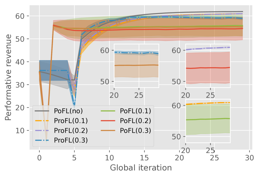
(a) Depend on Learning Rates

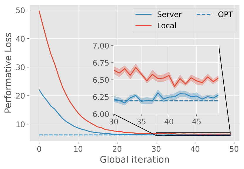
(b) Estimation on Server

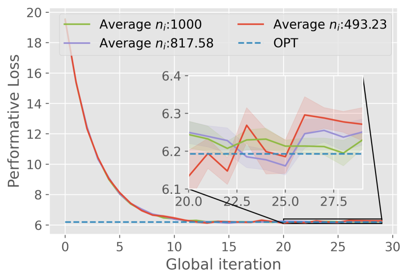
(c) Adaptive Learning Rate

Figure 1: Effectiveness of Proposed methods

(a) Different Sample Sizes

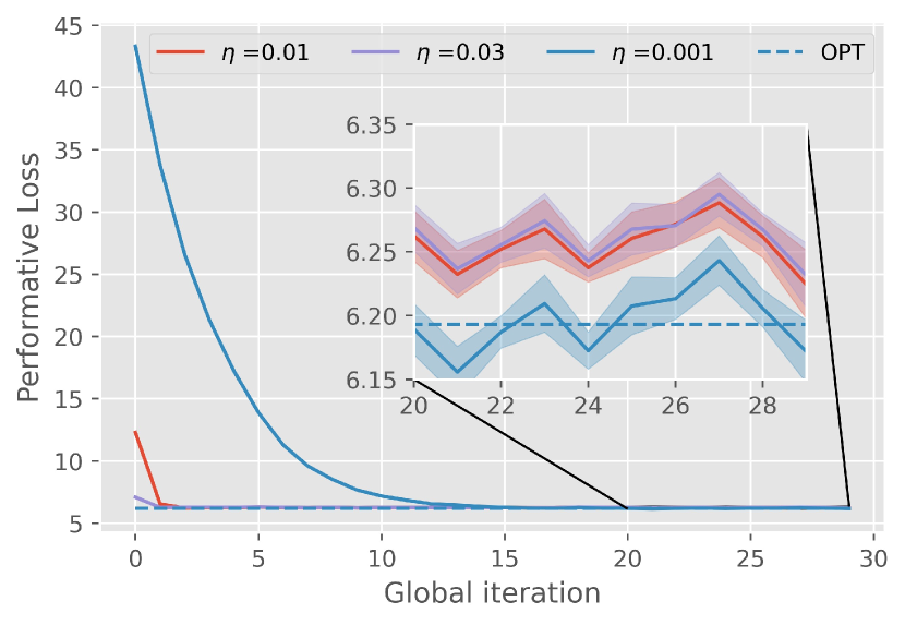
(b) Different Learning Rates

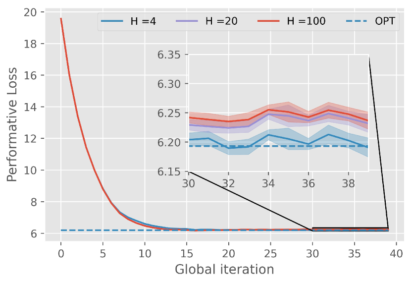
(c) Different H

Figure 2: Dynamic contribution with Different Sample Sizes, Learning Rates, and $H$

Comparison to Centralized Setting. Table 1 shows that adapting performative gradients to the FL framework improves performance. There are 10 clients with $\gamma_{i}\in[\overline{\gamma}-\alpha,\overline{\gamma}+\alpha]$, where larger $\alpha$ indicates more heterogeneity. As client heterogeneity increases, the performance of both algorithms degrades. Under homogeneous distribution shifts ($\alpha=0$), both algorithms perform similarly. ProFL (ours) outperforms PG when $\alpha=0.25$ or $\alpha=0.5$, as the centralized approach struggles to handle variance shifts by estimating a single $\frac{df}{d\theta}$ on the server.

Effectiveness of our proposed methods. Fig. 1(a) shows that contamination can significantly degrade performance, but the proposed robust gradient can effectively reduce the impact of contaminated data when computing the gradients i.e., the performance with the robust gradient in our method is almost the same as the case when outliers do not exist at all. This case study, pricing with dynamic demands, involves 10 heterogeneous clients with different $D_{i}(\theta)$, each encounters an $\epsilon_{i}$ fraction of contaminated data from a fixed but unknown exogenous distribution $Q_{i}$. Although we present the results when $Q_{i}\sim\mathcal{N}(\mu_{o},\sigma^{2}_{o})$, we observed similar results when $Q_{i}$ follows other distributions and are different among clients.

Fig. 1(b) shows that with a limited sample size and many clients ($n_{i}=60,|\mathcal{V}|=100$), estimating $\widehat{\frac{df_{i}}{d\theta}}$ on the server side results in a lower loss value compared to local estimation and approaches the optimal value. Fig. 1(c) demonstrates the effectiveness of adaptive sample sizing. We tested two tolerances (0.05 for purple, 0.1 for red), with each client processing up to 1000 samples per iteration. The adaptive approach significantly reduces the sample size while achieving similar results within the error tolerance, leading to substantial computational savings. Both experiments are based on the case study pricing with dynamic contribution, involving a non-linear $f_{i}(\theta)$.

Impact of hyperparameters. We examine the effects of sample size $n_{i}$, learning rate $\eta$, and estimation window $H$. Fig. 2(a) shows that increasing $n_{i}$ improves stability and brings the algorithm closer to the optimal point. Fig. 2(b) indicates that a smaller $\eta$ slows convergence but moves $\theta$ nearer to the optimum. Fig. 2(c) demonstrates that a smaller $H$ results in estimates estimates of $\frac{df_{i}}{d\theta}$ based on closer but smaller groups of $\widehat{f_{i}}$ and $\theta_{i}$, resulting in convergence closer to the performative optimum, albeit at a slightly slower speed.

Table 2: Accuracy of Binary Classification on Synthetic and Realistic Datasets

DATASET	POFL	PROFL
Same Distribution	88.00 $\pm$ 2.69	99.23 $\pm$ 0.29
Different Distributions	62.44 $\pm$ 0.52	92.50 $\pm$ 0.29
Credit Dataset	94.73 $\pm$ 0.00	94.73 $\pm$ 0.00
Adult Dataset	54.74 $\pm$ 0.02	60.78 $\pm$ 0.81

Convergence to the performative optimal solution. Table 2 shows that ProFL outperforms PFL in the case study of binary strategic classification with 10 heterogeneous clients. Since PFL cannot handle contaminated data, we set $\epsilon_{i}=0$ for these experiments. The first two rows show that ProFL is more stable and significantly more accurate than PFL on Gaussian synthetic data. PFL converges to a PS point rather than a PO point. On the Give Me Some Credit dataset (third row), both algorithms converge to the same point, but ProFL has a faster convergence rate (see Fig. 7(c) in the Appendix). With the Adult dataset, ProFL achieves $60.78\%$ accuracy, outperforming PFL’s $54.74\%$. These results highlight ProFL’s practical advantages in both convergence speed and accuracy. More results are in Appendix D.1.

Appendix A Algorithms and Details

A.1 Pseudocode of the PoFL

Algorithm 2 presents the pseudocode of the PoFL algorithm discussed in the main paper.

Algorithm 2 PoFL

1:  Input: Learning rate $\eta$, estimation window $H$, function $\widehat{f}$, total iterations $T$, local update iterations $R$.

2:  for $t=0$ to $T-1$ do

3:     If $t\mod R=0$, server sends $\overline{\theta}^{t}$ to a selected set $\mathcal{I}_{t}\subseteq\mathcal{V}$ of clients and client $i\in\mathcal{I}_{t}$ sets the local model $\theta^{t}_{i}=\overline{\theta}^{t}$; otherwise $\mathcal{I}_{t}=\mathcal{I}_{t-1}.$

4:     for $i\in\mathcal{I}_{t}$ in parallel do

5:        Deploy $\theta^{t}_{i}$ and local environment changes and draw $n_{i}$ samples $\mathcal{S}_{i}:=(z_{j})^{n_{i}}_{j=1}\mathop{\sim}\limits^{iid}P_{i}(\theta^{t}_{i})$.

6:        if $t\leq H$ then

7:           Compute estimator $\widehat{f}\left(\mathcal{S}_{i}\right)$ of $f^{t}_{i}$.

8:           Update $\theta^{t+1}_{i}\leftarrow\text{Proj}_{\Theta}\left(\theta^{t}_{i}-\eta\widehat{\nabla}\mathcal{L}_{i,1}(\theta^{t}_{i})\right)$.

9:        else

10:           Compute estimator $\widehat{f}\left(\mathcal{S}_{i}\right)$ of $f^{t}_{i}$.

11:           Form matrices $\Delta\theta_{i}$ and $\Delta f_{i}$ and compute $\Delta f_{i}(\Delta\theta_{i})^{\dagger}$.

12:           $\theta^{t+1}_{i}\leftarrow\text{Proj}_{\Theta}\left(\theta^{t}_{i}-\eta\left(\widehat{\nabla}\mathcal{L}_{i,1}(\theta^{t}_{i})+\widehat{\nabla}\mathcal{L}_{i,2}(\theta^{t}_{i})\right)\right)$.

13:     If $t\mod R=0$, client $i\in\mathcal{I}_{t}$ sends $\theta^{t}_{i}$ to the server and server updates the model $\overline{\theta}^{t+1}=\sum_{i\in\mathcal{I}_{t}}\alpha_{i}\theta^{t+1}_{i}$.

14:  Output: $\overline{\theta}^{T}$

Algorithm 3 Robust Gradient

1:  Input: Set $\mathcal{S}_{i}$ of samples $(z_{j})_{j=1}^{n_{i}}$, thresholds $C,J\in(0,1)$, model $\theta^{t}_{i}\in\Theta$

2:  Let $\widehat{\nabla}\leftarrow\frac{1}{|\mathcal{S}_{i}|}\sum_{z_{j}\in\mathcal{S}_{i}}\nabla\ell(z_{j};\theta^{t}_{i})$.

3:  Let $\left[\nabla\ell(z_{j};\theta^{t}_{i})-\widehat{\nabla}\right]_{z_{j}\in\mathcal{S}_{i}}$ be the $|\mathcal{S}_{i}|\times d$ matrix of centered gradients.

4:  Apply SVD to this matrix and find top right singular vector $v$.

5:  Compute the outlier score $\tau_{j}$ of $\nabla\ell(z_{j};\theta^{t}_{i})$ by Eq. (9).

6:  Divide the interval $[0,\max\tau_{j}]$ into $B$ equal-length segments. Let $\phi_{k}$ be the number of $\tau_{j}$ in the $k$-th segment.

7:  Find the smallest $k\in\{1,\cdots,B\}$ with $\phi_{k}<C\cdot|\mathcal{S}_{i}|$. Set $\phi$ as the lower bound of the $k$-th segment.

8:  Find the set $\mathcal{S}_{i}^{\prime}\leftarrow\{z_{j}\in\mathcal{S}_{i}:\tau_{j}<\phi\}$.

9:  Compare the average gradients $\widehat{\nabla}$ of $\mathcal{S}_{i}$ and $\widehat{\nabla}^{\prime}$ of $\mathcal{S}^{\prime}_{i}$. If $\frac{\|\widehat{\nabla}-\widehat{\nabla}^{\prime}\|}{\|\widehat{\nabla}\|}<J$ or $|\mathcal{S}^{\prime}_{i}|\leq\frac{n_{i}}{2}$, return $\mathcal{S}^{\prime}_{i}$ and $\widehat{\nabla}^{\prime}$; otherwise, set $\mathcal{S}_{i}\leftarrow\mathcal{S}^{\prime}_{i}$ and repeat from line 2.

A.2 Outlier removal mechanism for robust gradient

To estimate $\nabla\mathcal{L}_{i,1}$, we should average $\nabla\ell(z_{j};\theta_{i}^{t})$ over samples drawn from $D_{i}({\theta}_{i}^{t})$. Because the samples collected by client $i$ in round $t$ are drawn from $P_{i}(\theta_{i}^{t})$, they are noisy, with an unknown $\epsilon_{i}$ fraction of outliers from an unknown distribution $Q_{i}$. ProFL needs to identify contaminated data and eliminate the corresponding contaminated gradients. We propose a mechanism that can remove these contaminated gradients and estimate gradients that are robust to outliers. Importantly, ProFL is independent of the specific outlier identification and removal mechanism used and can function with any such mechanism. In our paper, we assume that contaminated data can follow an arbitrary distribution. In practice, additional information about the contamination process may be available based on the application or context, allowing us to design more efficient (and less expensive) outlier identification mechanisms leveraging this knowledge.

As shown in Algorithm 3, our mechanism takes noisy samples $\mathcal{S}_{i}$ and current local model $\theta_{i}^{t}$ as inputs. The mechanism first computes the gradients $\nabla\ell(z_{j};\theta_{i}^{t})$ of all samples and iteratively identifies and removes the contaminated gradients.

Since both the distribution $Q_{i}$ and fraction $\epsilon_{i}$ of contaminated data are unknown, we consider gradients contaminated if they exhibit two crucial properties: 1) they have large effects on the learned model and can disturb the training process (i.e., gradients have large magnitudes and systematically point in a specific direction); 2) they are located farther away from the average in the vector space (i.e., “long tail” data). To detect gradients that satisfy these properties, we adapt the approach in Shan et al., (2023), which leverages singular value decomposition (SVD). Instead of preselecting the threshold for the sum of all outlier scores $\tau_{j}$, which is difficult to determine without any prior knowledge of the data, our threshold is based on the two crucial properties, making it much easier to predict the values of $C$ and $J$. Specifically, we construct a matrix $[\nabla\ell(z_{j};\theta^{t}_{i})-\widehat{\nabla}]_{z_{j}\in\mathcal{S}_{i}}$ using the centered gradients and find the top right singular vector $v$, where $\widehat{\nabla}$ represents the average of all gradients (lines 2-4). The centered gradients that are closer to $v$ are more likely to be outliers and we assign each gradient an outlier score $\tau_{j}$ as follows:

$$\tau_{j}={\left(\left(\nabla\ell(z_{j};\theta^{t}_{i})-\widehat{\nabla}\right)^{T}v\right)}^{2}$$ (9)

Given the outlier scores $\{\tau_{j}\}$, the gradients with scores above a threshold $\phi$ are considered contaminated and are discarded. Unlike Shan et al., (2023) that uses a fixed pre-defined threshold, our method finds $\phi$ automatically based on the outlier score distribution. Since we assume the outliers are in the “long tail” of the distribution, we divide the interval $[0,\max\tau_{j}]$ into $B$ equal-length segments and compute the relative frequency distribution of scores. $\phi$ is set as the smallest segment with the relative frequency below a threshold (lines 6-7). For the remaining gradients with $\tau_{j}<\phi$, we compute their average $\widehat{\nabla}^{\prime}$ (lines 8-9).

Appendix B Additional Related Work

B.1 Performative Prediction in Centralized Settings

Performative prediction (Perdomo et al.,, 2020) was first introduced in 2020 corresponding to the optimization framework to deal with endogenous data distribution shifts where the model deployed to the environment will affect the subsequent data, resulting in the collected data changing as the deployed model changes. Common applications of performative prediction include strategic classification(Hardt et al.,, 2016; Xie and Zhang,, 2024) and predictive policing (Ensign et al.,, 2018). Perdomo et al., (2020) first proposes an iterative optimization procedure named Repeated Risk Minimizationto find a performative stable point and also bounded the distance between the performative stable point and the performative optimal point. Mendler-Dünner et al., (2020) designed the first algorithm to find the performative stable point under the online learning setting. Miller et al., (2021) first solved the problem of performative prediction by directly optimizing performance risk to find the performative optimal point, but the scope of the distribution map is restricted. Mendler-Dünner et al., (2022) proved the convergence of greedy deployment and lazy deployment after each random update under the assumption of smoothness and strong convexity and gave the convergence rate. Izzo et al., (2021) also designed an algorithm performative gradient descent for finding the performative optimal solution. Zhao, (2022) relaxes the assumption of strong convexity to the weakly-strongly convex case and proves the convergence of the deployment. Somerstep et al., (2024); Bracale et al., (2024) focused on learning the distribution map in performative prediction and proposed a framework named Reverse Causal Performative Prediction. In addition, performative prediction is also related to reinforcement learning(Zheng et al.,, 2022) and bandit problems(Chen et al.,, 2024).

B.2 Performative Prediction in Distributed System

To the best of our knowledge, Jin et al., (2024) is the only work discussing performativity under the distributed setting, where they generalized Fedavg to P-Fedavg and proved the uniqueness of the performative stable solution found by the algorithm. They also quantified the distance between the performative stable solution and the performative optimal solution. While the work is a breakthrough as the first to take model-dependent distribution shifts into account under the FL setting, it is only a strict generalization of Perdomo et al., (2020) without the ability to find the performative optimal point and deal with the contaminated data.

B.3 Federated Learning under Dynamic Data

Previous works (Tan et al.,, 2023; Li et al., 2020a, ) pointed out that the training paradigm of FedAvg may violate the i.i.d. assumptions and cause some feature classes to be over-represented while others to be under-represented. Li et al., 2020b ; Li et al., (2021) steer the local models towards a global model by adding a regularization term to guarantee convergence when the data distributions among different clients are non-IID. Li et al., 2020b proposes FedProx as a solution. Li et al., (2021) aims at obtaining good local models on clients rather than a global consensus model. Meanwhile, another line of work focused on dealing with the statistical heterogeneity by clustering (Briggs et al.,, 2020; Ghosh et al.,, 2020; Sattler et al.,, 2020) by aggregating clients with similar distribution into the same cluster. While most previous works assumed the “dynamic” is among different clients, another line of literature focuses on FL in a dynamic environment where various distribution shifts occur. Some works aim to deal with time-varying contribution rates of clients with local heterogeneity (Sattler et al.,, 2021; Park et al.,, 2021; Wang and Ji,, 2022; Zhu et al.,, 2021).

B.4 Huber’s $\epsilon$-contamination Model

Proposed by Huber, (1992), Huber’s epsilon contamination model serves as a framework for robust statistical analysis with outliers and contaminations in the dataset. This model assumes that besides the data distribution we aim to learn, a small proportion of samples can come from an arbitrary distribution. This contamination framework is crucial for creating machine learning algorithms robust to outliers, thereby ensuring more reliable analysis in practical scenarios where data imperfections are common. Huber’s model has been fundamental in the field of robust statistics, influencing a wide range of applications and subsequent research. Specifically, denote $D$ as the true data distribution and $Q$ as a random distribution. $P=(1-\epsilon)D+Q$ is the distribution with some corruption $Q$ and the portion of corruption data is $\epsilon$. The local dataset of client $i$ is $P_{i}=(1-\epsilon_{i})D_{i}(\theta_{i})+\epsilon_{i}Q_{i}$.

Appendix C Additional Proofs not Detailed in the Main Paper

C.1 Proof of Theorem 5.10

Proof.

With Assumption 5.1 of $\gamma_{i}$-sensitivity and Assumption 5.2 of $L$-smoothness, we obtain

$$\|\nabla\ell(z;\mathbf{\theta})-\nabla\ell(z^{\prime};\mathbf{\theta^{\prime}})\|\leq L(\|\mathbf{\theta}-\mathbf{\theta^{\prime}}\|+\|z-z^{\prime}\|)\leq L(1+\gamma_{i})\|\mathbf{\theta}-\mathbf{\theta^{\prime}}\|$$

Then we have

$$\mathcal{L}(\overline{\theta}^{t+1})\leq\mathcal{L}(\overline{\theta}^{t})+\langle\nabla\mathcal{L}(\overline{\theta}^{t}),\overline{\theta}^{t+1}-\overline{\theta}^{t}\rangle+\frac{L\sum^{N}_{i=1}\alpha_{i}(1+\gamma_{i})}{2}{\|\overline{\theta}^{t+1}-\overline{\theta}^{t}\|}^{2},$$

where $\overline{\theta}^{t+1}-\overline{\theta}^{t}=-g^{t}\eta$ and $g^{t}=\sum_{i=1}^{N}\alpha_{i}g^{t}_{i}$.

By taking expectation on both sides we obtain that

$$\mathbb{E}[\mathcal{L}(\overline{\theta}^{t+1})]$$

$$\leq\mathbb{E}[\mathcal{L}(\overline{\theta}^{t})]+\mathbb{E}\left[\langle\nabla\mathcal{L}(\overline{\theta}^{t}),\overline{\theta}^{t+1}-\overline{\theta}^{t}\rangle\right]+\frac{L\sum_{i=1}^{N}\alpha_{i}(1+\gamma_{i})}{2}\mathbb{E}\left[\|\overline{\theta}^{t+1}-\overline{\theta}^{t}\|^{2}\right]$$

$$=\mathbb{E}[\mathcal{L}(\overline{\theta}^{t})]\underbrace{-\mathbb{E}\left[\langle\nabla\mathcal{L}(\overline{\theta}^{t}),g^{t}\rangle\right]}_{T_{1}}\eta+\frac{L\sum_{i=1}^{N}\alpha_{i}(1+\gamma_{i})}{2}\underbrace{\mathbb{E}\left[\|g^{t}\|^{2}\right]}_{T_{2}}\eta^{2}.$$ (10)

Let’s start to find the upper bound of $T_{2}$. With $R$ steps local updates, by using Jensen’s inequality, we obtain that

$$\mathbb{E}\left[\|g^{t}\|^{2}\right]$$

$$=\mathbb{E}\left[\left\|\sum^{N}_{i=1}\alpha_{i}g^{t}_{i}\right\|^{2}\right]$$

$$\leq\mathbb{E}\left[\left\|\sum^{N}_{i=1}\alpha_{i}\left(g^{t}_{i}-\nabla\mathcal{L}_{i}(\theta^{t}_{i})+\nabla\mathcal{L}_{i}(\theta^{t}_{i})\right)\right\|^{2}\right]$$

$$\leq 2\mathbb{E}\left[\left\|\sum^{N}_{i=1}\alpha_{i}\left(g^{t}_{i}-\nabla\mathcal{L}_{i}(\theta^{t}_{i})\right)\right\|^{2}\right]+2\mathbb{E}\left[\left\|\sum^{N}_{i=1}\alpha_{i}\nabla\mathcal{L}_{i}(\theta^{t}_{i})\right\|^{2}\right]$$

$$\leq 2\mathbb{E}\left[\left\|\sum^{N}_{i=1}\alpha_{i}\left(g^{t}_{i}-\nabla\mathcal{L}_{i}(\theta^{t}_{i})\right)\right\|^{2}\right]+2G^{2}.$$

Then we start to find the upper bound of $T_{1}$.

$$-\mathbb{E}\left[\langle\nabla\mathcal{L}(\overline{\theta}^{t}),g^{t}\rangle\right]$$

$$=-\frac{1}{2}\mathbb{E}\left[\left\|\nabla\mathcal{L}(\overline{\theta}^{t})\right\|^{2}\right]-\frac{1}{2}\mathbb{E}\left[\left\|g^{t}\right\|^{2}\right]+\frac{1}{2}\mathbb{E}\left[\left\|\nabla\mathcal{L}(\overline{\theta}^{t})-g^{t}\right\|^{2}\right]$$

$$=-\frac{1}{2}\mathbb{E}\left[\left\|\nabla\mathcal{L}(\overline{\theta}^{t})\right\|^{2}\right]-\frac{1}{2}\mathbb{E}\left[\left\|g^{t}\right\|^{2}\right]+\frac{1}{2}\mathbb{E}\left[\left\|\nabla\mathcal{L}(\overline{\theta}^{t})-\sum^{N}_{i=1}\alpha_{i}\nabla\mathcal{L}_{i}({\theta}^{t}_{i})+\sum^{N}_{i=1}\alpha_{i}\nabla\mathcal{L}_{i}({\theta}^{t}_{i})-g^{t}\right\|^{2}\right]$$

$$\leq-\rho\mathbb{E}\left[\mathcal{L}(\overline{\theta}^{t})-\mathcal{L}(\overline{\theta}^{\text{PO}})\right]-\frac{1}{2}\mathbb{E}\left[\left\|g^{t}\right\|^{2}\right]+\mathbb{E}\left[\left\|\sum^{N}_{i=1}\alpha_{i}\left(\nabla\mathcal{L}_{i}(\overline{\theta}^{t})-\nabla\mathcal{L}_{i}({\theta}^{t}_{i})\right)\right\|^{2}\right]+\mathbb{E}\left[\left\|\sum^{N}_{i=1}\alpha_{i}\nabla\mathcal{L}_{i}({\theta}^{t}_{i})-g^{t}\right\|^{2}\right]$$

$$\leq-\rho\mathbb{E}\left[\mathcal{L}(\overline{\theta}^{t})-\mathcal{L}(\overline{\theta}^{\text{PO}})\right]-\frac{1}{2}\mathbb{E}\left[\left\|g^{t}\right\|^{2}\right]+L^{2}\mathbb{E}\left[\sum_{i=1}^{N}\alpha_{i}(1+\gamma_{i})^{2}\left\|\overline{\theta}^{t}-{\theta}^{t}_{i}\right\|^{2}\right]+\mathbb{E}\left[\left\|\sum^{N}_{i=1}\alpha_{i}\nabla\mathcal{L}_{i}({\theta}^{t}_{i})-g^{t}\right\|^{2}\right]$$

$$\leq-\rho\mathbb{E}\left[\mathcal{L}(\overline{\theta}^{t})-\mathcal{L}(\overline{\theta}^{\text{PO}})\right]-\frac{1}{2}\mathbb{E}\left[\left\|g^{t}\right\|^{2}\right]+L^{2}(R-1)^{2}G^{2}\eta^{2}\left((1+\overline{\gamma})^{2}+\sigma^{2}_{\gamma}\right)+\mathbb{E}\left[\left\|\sum^{N}_{i=1}\alpha_{i}\nabla\mathcal{L}_{i}({\theta}^{t}_{i})-g^{t}\right\|^{2}\right].$$

The first inequality arises from the application of Jensen’s inequality to two terms. The second inequality arises from Assumption 5.2. The last inequality arises form Lemma C.1.

Finally, bring $T_{1}$ and $T_{2}$ into Eq. (10) and subtract $\mathcal{L}(\overline{\theta}^{\text{PO}})$ from both sides, we can get that

$$\mathbb{E}[\mathcal{L}(\overline{\theta}^{t+1})-\mathcal{L}({\theta}^{\text{PO}})]$$

$$\leq(1-\rho\eta)\mathbb{E}[\mathcal{L}(\overline{\theta}^{t})-\mathcal{L}({\theta}^{\text{PO}})]+\frac{L^{2}(R-1)^{2}G^{2}\eta^{3}}{2}\left((1+\overline{\gamma})^{2}+\sigma^{2}_{\gamma}\right)+LG^{2}\eta^{2}(1+\overline{\gamma})$$

$$+L\eta^{2}(1+\overline{\gamma})\mathbb{E}\left[\left\|\sum^{N}_{i=1}\alpha_{i}\nabla\mathcal{L}_{i}({\theta}^{t}_{i})-g^{t}\right\|^{2}\right]+\mathbb{E}\left[|\left\|\sum^{N}_{i=1}\alpha_{i}\nabla\mathcal{L}_{i}({\theta}^{t}_{i})-g^{t}\right\|^{2}-\frac{1}{2}\left\|g^{t}\right\|^{2}\right]\eta,$$

where $\overline{\gamma}=\sum^{N}_{i=1}\alpha_{i}\gamma_{i}$ and $\sigma^{2}_{\gamma}=\sum^{N}_{i=1}\alpha_{i}(\overline{\gamma}-\gamma_{i})^{2}$.

Denote $\mathbb{E}[\mathcal{L}(\overline{\theta}^{t})-\mathcal{L}({\theta}^{\text{PO}})]$ as $a_{t}$. Then we can obtain that

$$a_{t+1} \leq(1-\rho\eta)a_{t}+\frac{L^{2}(R-1)^{2}G^{2}\eta^{3}}{2}\left((1+\overline{\gamma})^{2}+\sigma^{2}_{\gamma}\right)$$

$$\quad+LG^{2}\eta^{2}(1+\overline{\gamma})+L\eta^{2}(1+\overline{\gamma})\mathbb{E}\left[\left\|\sum^{N}_{i=1}\alpha_{i}\nabla\mathcal{L}_{i}({\theta}^{t}_{i})-g^{t}\right\|^{2}\right]$$

$$\quad+\mathbb{E}\left[\left\|\sum^{N}_{i=1}\alpha_{i}\nabla\mathcal{L}_{i}({\theta}^{t}_{i})-g^{t}\right\|^{2}-\frac{1}{2}\left\|g^{t}\right\|^{2}\right]\eta$$

$$=(1-\rho\eta)a_{t}+\underbrace{\mathbb{E}\left[\left\|\sum^{N}_{i=1}\alpha_{i}\nabla\mathcal{L}_{i}({\theta}^{t}_{i})-g^{t}\right\|^{2}-\frac{1}{2}\left\|g^{t}\right\|^{2}\right]}_{T_{4}}\eta$$

$$\quad+\underbrace{\frac{1}{2}\left(L^{2}(R-1)^{2}G^{2}\eta\left((1+\overline{\gamma})^{2}+\sigma^{2}_{\gamma}\right)+2LG^{2}(1+\overline{\gamma})+2L(1+\overline{\gamma})\mathbb{E}\left[\left\|\sum^{N}_{i=1}\alpha_{i}\nabla\mathcal{L}_{i}({\theta}^{t}_{i})-g^{t}\right\|^{2}\right]\right)}_{T_{3}}\eta^{2}.$$ (11)

Denote the empirical result of the performative gradient of client $i$ in global iteration $t$ and local iteration $r$ as $\hat{\nabla}\mathcal{L}_{i}(\theta_{i}^{t})=\hat{\nabla}\mathcal{L}_{i,1}(\theta_{i}^{t})+\hat{\nabla}\mathcal{L}_{i,2}(\theta_{i}^{t})$. According to Lemma C.2, we have

$$\mathbb{E}\left[\left\|\sum^{N}_{i=1}\alpha_{i}\nabla\mathcal{L}_{i}({\theta}^{t}_{i})-g^{t}\right\|^{2}\right] \leq\sum^{N}_{i=1}\alpha_{i}\mathbb{E}\left[\left\|\nabla\mathcal{L}_{i}(\theta_{i}^{t})-g_{i}^{t}\right\|^{2}\right]$$

$$\leq(1-\overline{\epsilon})\overline{\boldsymbol{\omega_{D}}}^{2}+\overline{\epsilon}\left(LW_{1}\left(D,Q\right)_{\max}+\overline{\boldsymbol{\omega_{Q}}}+\overline{\boldsymbol{\omega_{D}}}\right)^{2}.$$

where $\overline{\epsilon}=\sum^{N}_{i=1}\alpha_{i}\epsilon_{i},\sigma^{2}_{\epsilon}=\sum^{N}_{i=1}\alpha_{i}(\overline{\epsilon}-\epsilon_{i})^{2},$ and $\overline{\boldsymbol{\omega_{Q}}},\overline{\boldsymbol{\omega_{D}}}$ are the maximum of $\boldsymbol{\omega_{Q}}$ and $\boldsymbol{\omega_{D}}$ of all clients and all iterations. We can find the upper bound of $T_{3}$.

$$T_{3} \leq\frac{1}{2}\left(L^{2}(R-1)^{2}G^{2}\eta\left((1+\overline{\gamma})^{2}+\sigma^{2}_{\gamma}\right)+2LG^{2}(1+\overline{\gamma})+2L(1+\overline{\gamma})\mathbb{E}\left[\left\|\sum^{N}_{i=1}\alpha_{i}\nabla\mathcal{L}_{i}({\theta}^{t}_{i})-g^{t}\right\|^{2}\right]\right)$$

$$\leq\frac{1}{2}\left(L^{2}(R-1)^{2}G^{2}\eta\left((1+\overline{\gamma})^{2}+\sigma^{2}_{\gamma}\right)\right)+L(1+\overline{\gamma})\left((1-\overline{\epsilon})\overline{\boldsymbol{\omega_{D}}}^{2}+\overline{\epsilon}\left(LW_{1}\left(D,Q\right)_{\max}+\overline{\boldsymbol{\omega_{Q}}}+\overline{\boldsymbol{\omega_{D}}}\right)^{2}+G^{2}\right).$$

Let

$$C= \left(\frac{L^{2}(R-1)^{2}G^{2}\eta\left((1+\overline{\gamma})^{2}+\sigma^{2}_{\gamma}\right)}{2}+L(1+\overline{\gamma})\left((1-\overline{\epsilon})\overline{\boldsymbol{\omega_{D}}}^{2}+\overline{\epsilon}\left(LW_{1}\left(D,Q\right)_{\max}+\overline{\boldsymbol{\omega_{Q}}}+\overline{\boldsymbol{\omega_{D}}}\right)^{2}+G^{2}\right)\right)\eta^{2}$$

$$+\left((1-\overline{\epsilon})\overline{\boldsymbol{\omega_{D}}}^{2}+\overline{\epsilon}\left(LW_{1}\left(D,Q\right)_{\max}+\overline{\boldsymbol{\omega_{Q}}}+\overline{\boldsymbol{\omega_{D}}}\right)^{2}\right)\eta.$$

We will obtain

$$a_{t+1}\leq(1-\rho\eta)a_{t}+C$$

and

$$a_{t}\leq(1-\rho\eta)^{t}a_{0}+\frac{1-(1-\rho\eta)^{t}}{1-(1-\rho\eta)}C=(1-\rho\eta)^{t}a_{0}+\frac{1-(1-\rho\eta)^{t}}{\rho\eta}C\leq(1-\rho\eta)^{t}a_{0}+C,$$

which means

$$\mathbb{E}[\mathcal{L}(\overline{\theta}^{t})-\mathcal{L}({\theta}^{\text{PO}})]\leq(1-\rho\eta)^{t}\mathbb{E}[\mathcal{L}(\overline{\theta}^{0})-\mathcal{L}({\theta}^{\text{PO}})]+C.$$

∎

C.2 Proof of Lemma 5.7

Proof.

$\frac{\widehat{df}}{d\theta}$ is the estimate of $\frac{df}{d\theta}$. To simplify the notation in this proof we denote ${f_{i}}_{z\sim D_{i}(\theta^{t}_{i})}(z)$ as ${f_{t}}$ and $\nabla{f_{i}}_{z\sim D_{i}(\theta^{t}_{i})}(z)$ as $\nabla{f_{t}}$. $\widehat{f}_{t}$ is the estimate of $f(\theta).$ Because $\widehat{f}_{t}$ is estimated by data sampled from $P_{i}(\theta^{t}_{i})=(1-\epsilon_{i})D_{i}(\theta^{t}_{i})+\epsilon_{i}Q_{i}$ and we estimate the mean of mixture Gaussian or the $p$ of Binomial distribution $X\sim(n,p)$ we have

$$\widehat{f}_{r} =\widehat{f_{i}}_{z\sim P_{i}(\theta^{t}_{i})}(z)$$

$$=(1-\epsilon_{i})\widehat{f_{i}}_{z\sim D_{i}(\theta^{t}_{i})}(z)+\epsilon_{i}\widehat{f_{i}}_{z\sim Q_{i}}(z)$$

$$=(1-\epsilon_{i})\left({f_{i}}_{z\sim D_{i}(\theta^{t}_{i})}(z)+\text{err}^{t}_{i}\right)+\epsilon_{i}\widehat{f_{i}}_{z\sim Q_{i}}(z),$$

where $\text{err}^{t}_{i}$ is the error result in sampling of client $i$ on iteration $t$ and $[\text{err}^{t}_{i}]=0$ for all $t\in[0,T-1].$ Similarly we have denote $\theta^{t}_{i}$ as $\theta_{t}$ , $\theta^{t-1}_{i}$ as $\theta_{t-1}$ , $\text{err}^{t}_{i}$ as $\text{err}_{t}$ , and $\text{err}^{t-1}_{i}$ as $\text{err}_{t-1}.$

For each $1\leq j\leq d$ by an approximation of Taylor’s series (ignoring higher order terms), we obtain

$$f_{t,j}-f_{t-1,j}=\nabla f_{t-1,j}^{\intercal}(\theta_{t}-\theta_{t-1})+\frac{1}{2}(\theta_{t}-\theta_{t-1})^{\intercal}\nabla^{2}f_{i}(\xi_{t-1,j})(\theta_{t}-\theta_{t-1}),$$

where $\xi_{t-1,j}$ lies on the line segment joining $\theta_{t-1}$ and $\theta_{t}$.

Denote

$$a_{t-k,j}=\frac{1}{2}(\theta_{t-k+1}-\theta_{t-k})^{\intercal}\nabla^{2}f_{i}(\xi_{t-k,j})(\theta_{t-k+1}-\theta_{t-k})~{}~{}\text{ and }~{}~{}a_{k}=\begin{bmatrix}a_{t-k,1}\\ \vdots\\ a_{t-k,d}\end{bmatrix}$$

Then we have

$$f_{t}-f_{t-1}=\frac{df}{d\theta}(\theta_{t}-\theta_{t-1})+a_{1}.$$

By using the update rule of Algorithm 1 we obtain that

$$\widehat{f}_{t}-\widehat{f}_{t-1} =(1-\epsilon_{i})\left({f}_{t}-{f}_{t-1}\right)+\epsilon_{i}\left({f}_{z\sim Q_{i}}(z)-{f}_{z\sim Q_{i}}(z)\right)+(1-\epsilon_{i})(\text{err}_{t}-\text{err}_{t-1})$$

$$=(1-\epsilon_{i})\begin{bmatrix}f_{t,1}-f_{t-1,1}\\ \vdots\\ f_{t,d}-f_{t-1,d}\end{bmatrix}+(\text{err}_{t}-\text{err}_{t-1}).$$

Then we can write $\Delta_{1}f$ in terms of $\frac{df}{d\theta}$.

$$\Delta_{1}f=\widehat{f}_{t}-\widehat{f}_{t-1}=(1-\epsilon_{i})\left(\frac{df}{d\theta}(\theta_{t}-\theta_{t-1})+a_{1}+(\text{err}_{t}-\text{err}_{t-1})\right).$$

Similarly, we can obtain

$$\Delta_{k}f =\widehat{f}_{t}-\widehat{f}_{t-k}=\sum^{k}_{q=1}\left(\widehat{f}_{t-q+1}-\widehat{f}_{t-q}\right)$$

$$=(1-\epsilon_{i})\frac{df}{d\theta}(\theta_{t}-\theta_{t-k})+(1-\epsilon_{i})\frac{df}{d\theta}\sum^{k}_{q=1}a_{q}+(1-\epsilon_{i})(\text{err}_{t}-\text{err}_{t-k}),$$

where $1\leq k\leq H.$

Now we can get

$$\Delta f =\left[\begin{array}[]{ccc}\rule[-4.30554pt]{0.5pt}{10.76385pt}&&\rule[-4.30554pt]{0.5pt}{10.76385pt}\\ \Delta_{1}f&\ldots&\Delta_{H}f\\ \rule[-4.30554pt]{0.5pt}{10.76385pt}&&\rule[-4.30554pt]{0.5pt}{10.76385pt}\end{array}\right];$$

$$\Delta\theta =\left[\begin{array}[]{ccc}\rule[-4.30554pt]{0.5pt}{10.76385pt}&&\rule[-4.30554pt]{0.5pt}{10.76385pt}\\ \theta_{t}-\theta_{t-1}&\ldots&\theta_{t}-\theta_{t-H}\\ \rule[-4.30554pt]{0.5pt}{10.76385pt}&&\rule[-4.30554pt]{0.5pt}{10.76385pt}\end{array}\right]$$

$$=\left[\begin{array}[]{ccc}\rule[-4.30554pt]{0.5pt}{10.76385pt}&&\rule[-4.30554pt]{0.5pt}{10.76385pt}\\ \nabla\mathcal{L}_{z\sim P_{i}(\theta_{t-1})}(z,\theta_{t-1})&\ldots&\sum^{H}_{k=1}\nabla\mathcal{L}_{z\sim P_{i}(\theta_{t-k})}(z,\theta_{t-k})\\ \rule[-4.30554pt]{0.5pt}{10.76385pt}&&\rule[-4.30554pt]{0.5pt}{10.76385pt}\end{array}\right]\eta.$$

Define matrices

$$A=\left[\begin{array}[]{ccc}\rule[-4.30554pt]{0.5pt}{10.76385pt}&&\rule[-4.30554pt]{0.5pt}{10.76385pt}\\ a_{1}&\ldots&\sum^{H}_{k=1}a_{k}\\ \rule[-4.30554pt]{0.5pt}{10.76385pt}&&\rule[-4.30554pt]{0.5pt}{10.76385pt}\end{array}\right]~{}~{}\text{ and }~{}~{}E=\left[\begin{array}[]{ccc}\rule[-4.30554pt]{0.5pt}{10.76385pt}&&\rule[-4.30554pt]{0.5pt}{10.76385pt}\\ \text{err}_{t}-\text{err}_{t-1}&\ldots&\text{err}_{t}-\text{err}_{t-H}\\ \rule[-4.30554pt]{0.5pt}{10.76385pt}&&\rule[-4.30554pt]{0.5pt}{10.76385pt}\end{array}\right].$$

Then we can find the difference between $\frac{\widehat{df}}{d\theta}$ and $\frac{df}{d\theta}:$

$$\frac{\widehat{df}}{d\theta}-\frac{df}{d\theta}=\Delta f(\Delta\theta)^{\dagger}-\frac{df}{d\theta}=-\epsilon_{i}\frac{df}{d\theta}+(1-\epsilon_{i})A(\Delta\theta)^{\dagger}+(1-\epsilon_{i})E(\Delta\theta)^{\dagger}$$

and we can obtain that

$$\mathbb{E}\left[\left\|\frac{\widehat{df}}{d\theta}-\frac{df}{d\theta}\right\|^{2}\right]$$

$$=\mathbb{E}\left[\left\|-\epsilon_{i}\frac{df}{d\theta}+(1-\epsilon_{i})A(\Delta\theta)^{\dagger}+(1-\epsilon_{i})E(\Delta\theta)^{\dagger}\right\|^{2}\right]$$

$$=\mathbb{E}\left[\left\|-\epsilon_{i}\frac{df}{d\theta}+(1-\epsilon_{i})A(\Delta\theta)^{\dagger}\right\|^{2}\right]+(1-\epsilon_{i})^{2}\mathbb{E}\left[\left\|E(\Delta\theta)^{\dagger}\right\|^{2}\right]$$ (12)

$$\leq 2\epsilon_{i}^{2}\mathbb{E}\left[\left\|\frac{df}{d\theta}\right\|^{2}\right]+2(1-\epsilon_{i})^{2}\mathbb{E}\left[\left\|A(\Delta\theta)^{\dagger}\right\|^{2}\right]+(1-\epsilon_{i})^{2}\mathbb{E}\left[\left\|E(\Delta\theta)^{\dagger}\right\|^{2}\right]$$ (13)

$$\leq 2\epsilon_{i}^{2}\mathbb{E}\left[\left\|\frac{df}{d\theta}\right\|^{2}\right]+(1-\epsilon_{i})^{2}\left(2\mathbb{E}\left[\left\|A\right\|^{2}_{F}\right]+\mathbb{E}\left[\left\|E\right\|^{2}_{F}\right]\right)\left\|\Delta\theta^{\dagger}\right\|^{2}$$ (14)

$$\leq 2\epsilon_{i}^{2}\mathbb{E}\left[\left\|\frac{df}{d\theta}\right\|^{2}\right]+(1-\epsilon_{i})^{2}{2}\mathbb{E}\left[\sum_{k=1}^{H}\left\|\theta_{t}-\theta_{t-k}\right\|^{4}\left(\sum_{j=1}^{d}\left\|\nabla^{2}f_{i}(\xi_{t-k,j})\right\|^{2}\right)\right]\left\|\Delta\theta^{\dagger}\right\|^{2}$$

$$+(1-\epsilon_{i})^{2}\mathbb{E}\left[\sum_{k=1}^{H}\left\|\text{err}_{t}-\text{err}_{t-k}\right\|^{2}\right]\left\|\Delta\theta^{\dagger}\right\|^{2}$$

$$\leq 2\epsilon_{i}^{2}\left\|\frac{df}{d\theta}\right\|^{2}+\left(\frac{(1-\epsilon_{i})^{2}M^{2}\eta^{4}G^{4}H^{6}}{2}+(1-\epsilon_{i})^{2}\mathbb{E}\left[\sum_{k=1}^{H}\left\|\text{err}_{t}-\text{err}_{t-k}\right\|^{2}\right]\right)\left\|\Delta\theta^{\dagger}\right\|^{2}$$

$$\leq 2\epsilon_{i}^{2}\left\|\frac{df}{d\theta}\right\|^{2}+\left(\frac{(1-\epsilon_{i})^{2}M^{2}\eta^{4}G^{4}H^{6}}{2}+(1-\epsilon_{i})^{2}\mathbb{E}\left[\sum_{k=1}^{H}\left(\left\|\text{err}_{t}\right\|^{2}+\left\|\text{err}_{t-k}\right\|^{2}\right)\right]\right)\left\|\Delta\theta^{\dagger}\right\|^{2}$$ (15)

$$\leq 2\epsilon_{i}^{2}F^{2}+(1-\epsilon_{i})^{2}\left(\frac{M^{2}\eta^{4}G^{4}H^{6}}{2}+\frac{2Hd\left\|\text{err}\right\|^{2}_{i}}{\eta^{2}}\right)\lambda^{-2}_{i,\min}.$$ (16)

Where $\left\|.\right\|_{F}$ denotes the Frobenius norm. (12) and (15) arise from the property that $\mathbb{E}\left[\text{err}_{t}\right]=0$ for all $t\in[0,T]$ and $\text{err}_{t}$ is independent to $a_{k}$ and $\frac{df}{d\theta}$. (13) arises from Jensen’s inequality of two terms. (14) arises form the properties of matrix norm that if $A$ and $B$ are two matrix $\left\|AB\right\|\leq\left\|A\right\|\left\|B\right\|$ and $\left\|A\right\|\leq\left\|A\right\|_{F}.$ (16) arises form $\left\|\Delta\theta^{\dagger}\right\|\leq\left\|\Delta\theta\right\|^{-1}\leq\lambda^{-1}_{i,min}$, where $\lambda_{i,min}$ is the smallest singular values of $\Delta\theta$ of client $i$ for all $t\in[0,T]$ and $\left\|\text{err}\right\|^{2}_{i}$ is the maximum of $\left\|\text{err}_{t}\right\|^{2}$ for all $t\in[0,T]$. Because $\left\|\text{err}_{t}\right\|^{2}$ depends on the data distribution, the estimation methods, the number of samples $n_{i}$, as well as the probability $\varphi_{i}$ of $\mathbf{Pr}(\left\|\text{err}_{t}\right\|\leq 1-\varphi_{i})$, we use $f_{\varphi}(\varphi_{i};n_{i})$ to represent this term.

Finally we obtrain

$$\mathbb{E}\left[\left\|\frac{\widehat{df}}{d\theta}-\frac{df}{d\theta}\right\|^{2}\right]\leq 2\epsilon_{i}^{2}F^{2}+(1-\epsilon_{i})^{2}\left(\frac{M^{2}\eta^{4}G^{4}H^{6}}{2}+\frac{2Hdf_{\varphi}(\varphi_{i};n_{i})}{\eta^{2}}\right)\lambda^{-2}_{i,\min}.$$

∎

C.3 Proof of Lemma 5.9

Proof.

First we start to find the upper bound of $\mathbb{E}\left[\left\|\nabla\mathcal{L}_{i,2}(\theta_{i}^{t})-\widehat{\nabla}\mathcal{L}_{{i,2}z\sim D_{i}(\theta_{i}^{t})}(z,\theta_{i}^{t})\right\|^{2}\right].$

By Eq. 3 we obtain that

$$\mathbb{E}\left[\left\|\nabla\mathcal{L}_{i,2}(\theta_{i}^{t})-\widehat{\nabla}\mathcal{L}_{{i,2}z\sim D_{i}(\theta_{i}^{t})}(z,\theta_{i}^{t})\right\|^{2}\right]$$

$$=\mathbb{E}\left[\left\|\ell(Z_{i};\theta_{i}^{t}){\frac{df_{i,t}}{d\theta}}^{\intercal}\frac{\partial\log p\left(Z_{i};f_{i}(\theta_{i}^{t})\right)}{\partial f_{i}(\theta_{i}^{t})}-\widehat{\ell}(Z_{i};\theta_{i}^{t}){\frac{\widehat{df_{i,t}}}{d\theta}}^{\intercal}\frac{\partial\log p\left(Z_{i};\widehat{f}_{i}(\theta_{i}^{t})\right)}{\partial\widehat{f}_{i}(\theta_{i}^{t})}\right\|^{2}\right].$$

When the local client’s sample size $n_{i}\rightarrow\infty$, we have

$$\mathbb{E}\left[\left\|\ell(Z_{i};\theta)-\widehat{\ell}(Z_{i};\theta)\right\|^{2}\right]\rightarrow 0$$

$$\mathbb{E}\left[\left\|\frac{\partial\log p\left(Z_{i};f_{i}(\theta)\right)}{\partial f_{i}(\theta)}-\frac{\partial\log p\left(Z_{i};\widehat{f}_{i}(\theta)\right)}{\partial\widehat{f}_{i}(\theta)}\right\|^{2}\right]\rightarrow 0$$

Thereby, $\mathbb{E}\left[\left\|\ell(Z_{i};\theta_{i}^{t}){\frac{df_{i,t}}{d\theta}}^{\intercal}\frac{\partial\log p\left(Z_{i};f_{i}(\theta_{i}^{t})\right)}{\partial f_{i}(\theta_{i}^{t})}-\widehat{\ell}(Z_{i};\theta_{i}^{t}){\frac{\widehat{df_{i,t}}}{d\theta}}^{\intercal}\frac{\partial\log p\left(Z_{i};\widehat{f}_{i}(\theta_{i}^{t})\right)}{\partial\widehat{f}_{i}(\theta_{i}^{t})}\right\|^{2}\right]$ mainly includes two parts.

The first part is the following:

$$\mathbb{E}\left[\left\|\ell(Z_{i};\theta_{i}^{t})\right\|^{2}\left\|\frac{df_{i,t}}{d\theta}-\frac{\widehat{df_{i,t}}}{d\theta}\right\|^{2}\left\|\frac{\partial\log p\left(Z_{i};f_{i}(\theta_{i}^{t})\right)}{\partial f_{i}(\theta_{i}^{t})}\right\|^{2}\right]$$

$$\leq\ell^{2}_{\max}\left\|\frac{\partial\log p\left(Z_{i};f_{i}(\theta_{i}^{t})\right)}{\partial f_{i}(\theta_{i}^{t})}\right\|^{2}_{\max}\mathbb{E}\left[\left\|\frac{df_{i,t}}{d\theta}-\frac{\widehat{df_{i,t}}}{d\theta}\right\|^{2}\right]$$ (17)

$$=\mathcal{O}\left(\ell^{2}_{\max}d\left(\boldsymbol{\omega_{F}}\right)\right).$$ (18)

Because $\Theta$ is a closed and bounded set and a continuous function has a maximum value on $\Theta$, there is an upper bound $\ell^{2}_{\max}$ of $\left\|\ell(Z_{i};\theta)\right\|^{2}$ and an upper bound $\left\|\frac{\partial\log p\left(Z_{i};f_{i}(\theta_{i}^{t})\right)}{\partial f_{i}(\theta_{i}^{t})}\right\|^{2}_{\max}$ of $\left\|\frac{\partial\log p\left(Z_{i};f_{i}(\theta_{i}^{t})\right)}{\partial f_{i}(\theta_{i}^{t})}\right\|^{2}$. (18) arises from the upper bound of $\left\|\frac{\partial\log p\left(Z_{i};f_{i}(\theta_{i}^{t})\right)}{\partial f_{i}(\theta_{i}^{t})}\right\|^{2}$ is $\mathcal{O}(d)$ and it is related to the covariance $\Sigma$ of the data for the Gaussian distribution.

The second part will decrease to zero as $n_{i}\rightarrow 0.$ The upper bound of this part is $\mathcal{O}\left(\ell^{2}_{\max}dF^{2}f_{\varphi}(\varphi_{i};n_{i})\right)$ by using Lemma 12 in Izzo et al., (2021). Then we can obtain

$$\mathbb{E}\left[\left\|\nabla\mathcal{L}_{i,2}(\theta_{i}^{t})-\widehat{\nabla}\mathcal{L}_{{i,2}z\sim D_{i}(\theta_{i}^{t})}(z,\theta_{i}^{t})\right\|^{2}\right]\leq\mathcal{O}\left(\ell^{2}_{\max}d\left(\left(\boldsymbol{\omega_{F}}\right)+F^{2}f_{\varphi}(\varphi_{i};n_{i})\right)\right).$$

Next we find the upper bound of $\mathbb{E}\left[\left\|{\nabla}\mathcal{L}_{{i,2}}(Q_{i},\theta_{i}^{t})-\widehat{\nabla}\mathcal{L}_{{i,2}}(Q_{i},\theta_{i}^{t})\right\|^{2}\right].$

$$\mathbb{E}\left[\left\|{\nabla}\mathcal{L}_{{i,2}}(Q_{i},\theta_{i}^{t})-\widehat{\nabla}\mathcal{L}_{{i,2}}(Q_{i},\theta_{i}^{t})\right\|^{2}\right]$$

$$=\mathbb{E}\left[\left\|\widehat{\nabla}\mathcal{L}_{{i,2}}(Q_{i},\theta_{i}^{t})\right\|^{2}\right]$$

$$=\mathbb{E}\left[\left\|{\ell}_{z\sim Q_{i}}(Z_{i};\theta_{i}^{t}){\frac{\widehat{df_{i,t}}}{d\theta}}^{\intercal}\frac{\partial\log p\left(Z_{i};\widehat{f}_{i}(\theta_{i}^{t})\right)}{\partial\widehat{f}_{i}(\theta_{i}^{t})}\right\|^{2}\right]$$ (19)

$$\leq\mathcal{O}\left(\ell^{2}_{\max}d\mathbb{E}\left[\left\|\frac{\widehat{df_{i,t}}}{d\theta}\right\|^{2}\right]\right)$$ (20)

$$\leq\mathcal{O}\left(2\ell^{2}_{\max}d\left(\mathbb{E}\left[\left\|\frac{{df_{i,t}}}{d\theta}\right\|^{2}\right]+\mathbb{E}\left[\left\|\frac{df_{i,t}}{d\theta}-\frac{\widehat{df_{i,t}}}{d\theta}\right\|^{2}\right]\right)\right)$$ (21)

$$=\mathcal{O}\left(2\ell^{2}_{\max}d\left(\left(\boldsymbol{\omega_{F}}\right)+F^{2}\right)\right).$$ (22)

(19) arises from Eq. (3). (20) arises from Lemma 10 of Izzo et al., (2021) and Lemma 5.6. (21) arises from Jensen’s inequality of two terms. (22) arises from Lemma 5.7. ∎

C.4 Additional Lemmas and their Proofs

Lemma C.1.

Let $\overline{\gamma}=\sum^{N}_{i=1}\alpha_{i}\gamma_{i}$ and $\sigma^{2}_{\gamma}$ be the variance of $\gamma_{i}$ of all clients. Then $\mathbb{E}\left[\sum_{i=1}^{N}\alpha_{i}(1+\gamma_{i})^{2}\left\|\overline{\theta}^{t}-{\theta}^{t}_{i}\right\|^{2}\right]$ is upper bounded by $(R-1)^{2}G^{2}\eta^{2}\left((1+\overline{\gamma})^{2}+\sigma^{2}_{\gamma}\right)$.

Proof of Lemma C.1.

$$\mathbb{E}\left[\sum_{i=1}^{N}\alpha_{i}(1+\gamma_{i})^{2}\left\|\overline{\theta}^{t}-{\theta}^{t}_{i}\right\|^{2}\right] =\sum_{i=1}^{N}\alpha_{i}(1+\gamma_{i})^{2}\mathbb{E}\left[\left\|\overline{\theta}^{t}-{\theta}^{t}_{i}\right\|^{2}\right]$$

$$=\eta^{2}\sum_{i=1}^{N}\alpha_{i}(1+\gamma_{i})^{2}\mathbb{E}\left[\left\|\sum_{i=1}^{N}\alpha_{i}\sum_{j=t-b}^{t}\nabla\mathcal{L}_{i}({\theta}_{i}^{j})-\sum_{j=t-b}^{t}\nabla\mathcal{L}_{i}({\theta}_{i}^{j})\right\|^{2}\right]$$

$$\leq\eta^{2}\sum_{i=1}^{N}\alpha_{i}(1+\gamma_{i})^{2}\mathbb{E}\left[\left\|\sum_{j=t-b}^{t}\nabla\mathcal{L}_{i}({\theta}_{i}^{t})\right\|^{2}\right]$$

$$\leq c^{2}G^{2}\eta^{2}\sum_{i=1}^{N}\alpha_{i}(1+\gamma_{i})^{2}$$

$$\leq(R-1)^{2}G^{2}\eta^{2}\sum_{i=1}^{N}\alpha_{i}(1+\gamma_{i})^{2}.$$

$c=t\mod R$. The first inequality rises from $\mathbb{E}\left[\|\mathbb{E}[X]-X\|^{2}\right]\leq\mathbb{E}[X^{2}]$. The second inequality arises from Lemma 5.6 and Jensen’s inequality.

Denote $\sum^{N}_{i=1}\alpha_{i}\gamma_{i}$ as $\overline{\gamma}$ and variance of $\gamma_{i}$ as $\sigma^{2}_{\gamma}$. Because

$$\sum^{N}_{i=1}\alpha_{i}(1+\gamma_{i})^{2} =\mathbb{E}\left[(1+\gamma_{i})^{2}\right]$$

$$=\left(\mathbb{E}\left[1+\gamma_{i}\right]\right)^{2}+\mathbb{V}\left[1+\gamma_{i}\right]$$

$$=\left(\mathbb{E}\left[1+\gamma_{i}\right]\right)^{2}+\mathbb{V}\left[\gamma_{i}\right]=(1+\overline{\gamma})^{2}+\sigma^{2}_{\gamma}$$

we will finally obtain

$$\mathbb{E}\left[\sum_{i=1}^{N}\alpha_{i}(1+\gamma_{i})^{2}\left\|\overline{\theta}^{t}-{\theta}^{t}_{i}\right\|^{2}\right]\leq(R-1)^{2}G^{2}\eta^{2}\left((1+\overline{\gamma})^{2}+\sigma^{2}_{\gamma}\right).$$

∎

Lemma C.2.

If there is contaminated data with distribution $Q_{i}$ and fraction $\epsilon_{i}$ , with Assumption 5.2, we can obtain that

$$\mathbb{E}\left[\left\|\nabla\mathcal{L}_{i}(\theta_{i}^{t})-g_{i}^{t}\right\|^{2}\right]\leq(1-\epsilon_{i})(\boldsymbol{\omega_{D}})^{2}+\epsilon_{i}\left(LW_{1}\left(D,Q\right)_{\max}+(\boldsymbol{\omega_{Q}})+(\boldsymbol{\omega_{D}})\right)^{2}.$$

The notation $(\boldsymbol{\omega_{D}})$ and $(\boldsymbol{\omega_{Q}})$ is defined in Lemmas 5.8 and 5.9. $W_{1}\left(D,Q\right)_{\max}$ is the largest $W_{1}$ distance between $D_{i}(\theta)$ and $Q_{i}$ for all clients $i\in\mathcal{V}$ among all iteration $t\in[0,T-1]$.

Proof of Lemma C.2.

From Eq. (3) we can obtain

$$\nabla\mathcal{L}_{i}(\theta_{i}^{t})-g_{i}^{t}= \nabla\mathcal{L}_{i,1}(\theta_{i}^{t})-\widehat{\nabla}\mathcal{L}_{i,1}(\theta_{i}^{t})+\nabla\mathcal{L}_{i,2}(\theta_{i}^{t})-\widehat{\nabla}\mathcal{L}_{i,2}(\theta_{i}^{t})$$

$$= (1-\epsilon_{i})\left(\nabla\mathcal{L}_{i,1}(\theta_{i}^{t})-\widehat{\nabla}\mathcal{L}_{{i,1}}(D_{i}(\theta_{i}^{t}),\theta_{i}^{t})+\nabla\mathcal{L}_{i,2}(\theta_{i}^{t})-\widehat{\nabla}\mathcal{L}_{{i,2}}(D_{i}(\theta_{i}^{t}),\theta_{i}^{t})\right)$$

$$+\epsilon_{i}\left(\nabla\mathcal{L}_{i,1}(\theta_{i}^{t})-{\nabla}\mathcal{L}_{{i,1}}(Q_{i},\theta_{i}^{t})+\nabla\mathcal{L}_{i,2}(\theta_{i}^{t})-{\nabla}\mathcal{L}_{{i,2}}(Q_{i},\theta_{i}^{t})\right)$$

$$+\epsilon_{i}\left({\nabla}\mathcal{L}_{{i,1}z\sim Q_{i}}(z,\theta_{i}^{t})-\widehat{\nabla}\mathcal{L}_{{i,1}}(Q_{i},\theta_{i}^{t})+{\nabla}\mathcal{L}_{{i,2}}(Q_{i},\theta_{i}^{t})-\widehat{\nabla}\mathcal{L}_{{i,2}}(Q_{i},\theta_{i}^{t})\right)$$

$$= (1-\epsilon_{i})\left(\nabla\mathcal{L}_{i,1}(\theta_{i}^{t})-\widehat{\nabla}\mathcal{L}_{{i,1}}(D_{i}(\theta_{i}^{t}),\theta_{i}^{t})+\nabla\mathcal{L}_{i,2}(\theta_{i}^{t})-\widehat{\nabla}\mathcal{L}_{{i,2}}(D_{i}(\theta_{i}^{t}),\theta_{i}^{t})\right)$$

$$+\epsilon_{i}\left(\nabla\mathcal{L}_{i}(\theta_{i}^{t})-{\nabla}\mathcal{L}_{{i}z\sim Q_{i}}(z,\theta_{i}^{t})\right)-\epsilon_{i}\left(\widehat{\nabla}\mathcal{L}_{{i,2}z\sim Q_{i}}(z,\theta_{i}^{t})\right).$$

The last equality arises form ${\nabla}\mathcal{L}_{{i,1}}(Q_{i},\theta_{i}^{t})-\widehat{\nabla}\mathcal{L}_{{i,1}z\sim}(Q_{i},\theta_{i}^{t})=0\text{ and }{\nabla}\mathcal{L}_{{i,2}}(Q_{i},\theta_{i}^{t})=0$. Because $\mathbb{E}\left[\nabla\mathcal{L}_{i,1}(\theta_{i}^{t})-\widehat{\nabla}\mathcal{L}_{{i,1}}(D_{i}(\theta_{i}^{t}),\theta_{i}^{t})]\right]=0$ and Assumption 5.2 of $L$-smoothness.

The proof of the Lemma 12 of Izzo et al., (2021) shows that

$$\mathbb{E}\left[\left\|\nabla\mathcal{L}_{i,1}(\theta_{i}^{t})-\widehat{\nabla}\mathcal{L}_{{i,1}}(D_{i}(\theta_{i}^{t}),\theta_{i}^{t})\right\|^{2}\right]=\mathcal{O}\left(f_{\varphi}(\varphi_{i};n_{i})\right).$$

Finally, we can obtain that

$$\mathbb{E}\left[\left\|\nabla\mathcal{L}_{i}(\theta_{i}^{t})-g_{i}^{t}\right\|^{2}\right]$$

$$=(1-\epsilon_{i})^{2}\mathbb{E}\left[\left\|\nabla\mathcal{L}_{i,1}(\theta_{i}^{t})-\widehat{\nabla}\mathcal{L}_{{i,1}}(D_{i}(\theta_{i}^{t}),\theta_{i}^{t})\right\|^{2}\right]+(1-\epsilon_{i})^{2}\mathbb{E}\left[\left\|\nabla\mathcal{L}_{i,2}(\theta_{i}^{t})-\widehat{\nabla}\mathcal{L}_{{i,2}}(D_{i}(\theta_{i}^{t}),\theta_{i}^{t})\right\|^{2}\right]$$

$$+(1-\epsilon_{i})^{2}\epsilon_{i}\mathbb{E}\left[\left\langle\nabla\mathcal{L}_{i,1}(\theta_{i}^{t})-\widehat{\nabla}\mathcal{L}_{{i,1}}(D_{i}(\theta_{i}^{t}),\theta_{i}^{t}),\nabla\mathcal{L}_{i,2}(\theta_{i}^{t})-\widehat{\nabla}\mathcal{L}_{{i,2}}(D_{i}(\theta_{i}^{t}),\theta_{i}^{t})\right\rangle\right]$$

$$+\epsilon_{i}^{2}\mathbb{E}\left[\left\|\nabla\mathcal{L}_{i}(\theta_{i}^{t})-{\nabla}\mathcal{L}_{{i}}(Q_{i},\theta_{i}^{t})\right\|^{2}\right]+\epsilon_{i}^{2}\mathbb{E}\left[\left\|\widehat{\nabla}\mathcal{L}_{{i,2}}(Q_{i},\theta_{i}^{t})\right\|^{2}\right]$$

$$+2(1-\epsilon_{i})\epsilon_{i}\mathbb{E}\left[\left\langle\nabla\mathcal{L}_{i,2}(\theta_{i}^{t})-\widehat{\nabla}\mathcal{L}_{{i,2}}(D_{i}(\theta_{i}^{t}),\theta_{i}^{t}),\nabla\mathcal{L}_{i}(\theta_{i}^{t})-{\nabla}\mathcal{L}_{{i}}(Q_{i},\theta_{i}^{t})\right\rangle\right]$$

$$-2(1-\epsilon_{i})\epsilon_{i}\mathbb{E}\left[\left\langle\nabla\mathcal{L}_{i,2}(\theta_{i}^{t})-\widehat{\nabla}\mathcal{L}_{{i,2}}(D_{i}(\theta_{i}^{t}),\theta_{i}^{t}),\widehat{\nabla}\mathcal{L}_{{i,2}}(Q_{i},\theta_{i}^{t})\right\rangle\right]$$

$$-\epsilon^{2}_{i}\mathbb{E}\left[\left\langle\nabla\mathcal{L}_{i}(\theta_{i}^{t})-{\nabla}\mathcal{L}_{{i}}(Q_{i},\theta_{i}^{t}),\widehat{\nabla}\mathcal{L}_{{i,2}}(Q_{i},\theta_{i}^{t})\right\rangle\right]$$

$$\leq(1-\epsilon_{i})^{2}\mathbb{E}\left[\left\|\nabla\mathcal{L}_{i,1}(\theta_{i}^{t})-\widehat{\nabla}\mathcal{L}_{{i,1}}(D_{i}(\theta_{i}^{t}),\theta_{i}^{t})\right\|^{2}\right]+(1-\epsilon_{i})^{2}\mathbb{E}\left[\left\|\nabla\mathcal{L}_{i,2}(\theta_{i}^{t})-\widehat{\nabla}\mathcal{L}_{{i,2}}(D_{i}(\theta_{i}^{t}),\theta_{i}^{t})\right\|^{2}\right]$$

$$+(1-\epsilon_{i})^{2}\mathbb{E}\left[\left\|\nabla\mathcal{L}_{i,1}(\theta_{i}^{t})-\widehat{\nabla}\mathcal{L}_{{i,1}}(D_{i}(\theta_{i}^{t}),\theta_{i}^{t})\right\|\left\|\nabla\mathcal{L}_{i,2}(\theta_{i}^{t})-\widehat{\nabla}\mathcal{L}_{{i,2}}(D_{i}(\theta_{i}^{t}),\theta_{i}^{t})\right\|\right]$$

$$+\epsilon_{i}^{2}L^{2}\left\|D_{i}(\theta_{i}^{t})-Q_{i}\right\|^{2}+\epsilon_{i}^{2}\mathbb{E}\left[\left\|\widehat{\nabla}\mathcal{L}_{{i,2}}(Q_{i},\theta_{i}^{t})\right\|^{2}\right]$$

$$+2(1-\epsilon_{i})\epsilon_{i}L\left\|D_{i}(\theta_{i}^{t})-Q_{i}\right\|\mathbb{E}\left[\left\|\nabla\mathcal{L}_{i,2}(\theta_{i}^{t})-\widehat{\nabla}\mathcal{L}_{{i,2}}(D_{i}(\theta_{i}^{t}),\theta_{i}^{t})\right\|\right]$$

$$+2(1-\epsilon_{i})\epsilon_{i}\mathbb{E}\left[\left\|\nabla\mathcal{L}_{i,2}(\theta_{i}^{t})-\widehat{\nabla}\mathcal{L}_{{i,2}}(D_{i}(\theta_{i}^{t}),\theta_{i}^{t})\right\|\left\|\widehat{\nabla}\mathcal{L}_{{i,2}}(Q_{i},\theta_{i}^{t})\right\|\right]$$

$$+\epsilon^{2}_{i}L\left\|D_{i}(\theta_{i}^{t})-Q_{i}\right\|\mathbb{E}\left[\left\|\widehat{\nabla}\mathcal{L}_{{i,2}}(Q_{i},\theta_{i}^{t})\right\|\right]$$

$$\leq(1-\epsilon_{i})^{2}(\boldsymbol{\omega_{D}})^{2}+(1-\epsilon_{i})^{2}\mathcal{O}\left(f_{\varphi}(\varphi_{i};n_{i})\right)(\boldsymbol{\omega_{D}})+\epsilon_{i}^{2}\left(L^{2}W^{2}_{1}\left(D,Q\right)_{\max}+(\boldsymbol{\omega_{Q}})^{2}+W_{1}\left(D,Q\right)_{\max}(\boldsymbol{\omega_{Q}})\right)$$

$$+2(1-\epsilon_{i})\epsilon_{i}\left(LW_{1}\left(D,Q\right)_{\max}(\boldsymbol{\omega_{D}})+(\boldsymbol{\omega_{D}})(\boldsymbol{\omega_{Q}})\right)$$

The notation $(\boldsymbol{\omega_{D}})$ and $(\boldsymbol{\omega_{Q}})$ is defined in Lemma 5.9. $W_{1}\left(D,Q\right)_{\max}$ is the largest $W_{1}$ distance between $D_{i}(\theta)$ and $Q_{i}$ for all clients $i\in\mathcal{V}$ among all iteration $t\in[0,T-1]$. To simplify the upper bound first we use the fact that

$$(1-\epsilon_{i})^{2}(\boldsymbol{\omega_{D}})^{2}+(1-\epsilon_{i})^{2}\mathcal{O}(f_{\varphi}(\varphi_{i};n_{i}))(\boldsymbol{\omega_{D}})\approx(1-\epsilon_{i})^{2}(\boldsymbol{\omega_{D}})^{2}$$ (23)

because the estimation error of $\nabla\mathcal{L}_{i,1}$ is much smaller than $\nabla\mathcal{L}_{i,2}$ by using Lemmas 5.8 and 5.9. Apply the fact that $\epsilon_{i}\in[0,1]$ and we can obtain

$$(1-\epsilon_{i})^{2}(\boldsymbol{\omega_{D}})^{2}+(1-\epsilon_{i})^{2}\mathcal{O}\left(f_{\varphi}(\varphi_{i};n_{i})\right)(\boldsymbol{\omega_{D}})+\epsilon_{i}^{2}\left(L^{2}W^{2}_{1}\left(D,Q\right)_{\max}+(\boldsymbol{\omega_{Q}})^{2}+W_{1}\left(D,Q\right)_{\max}(\boldsymbol{\omega_{Q}})\right)$$

$$+2(1-\epsilon_{i})\epsilon_{i}\left(LW_{1}\left(D,Q\right)_{\max}(\boldsymbol{\omega_{D}})+(\boldsymbol{\omega_{D}})(\boldsymbol{\omega_{Q}})\right)$$

$$\leq(1-\epsilon_{i})(\boldsymbol{\omega_{D}})^{2}+\epsilon_{i}\left(L^{2}W^{2}_{1}\left(D,Q\right)_{\max}+(\boldsymbol{\omega_{Q}})^{2}+W_{1}\left(D,Q\right)_{\max}(\boldsymbol{\omega_{Q}})+LW_{1}\left(D,Q\right)_{\max}(\boldsymbol{\omega_{D}})+(\boldsymbol{\omega_{D}})(\boldsymbol{\omega_{Q}})\right)$$

$$\leq(1-\epsilon_{i})(\boldsymbol{\omega_{D}})^{2}+\epsilon_{i}\left(LW_{1}\left(D,Q\right)_{\max}+(\boldsymbol{\omega_{Q}})+(\boldsymbol{\omega_{D}})\right)^{2}.$$

∎

Lemma C.3 (Sensitivity of contribution Dynamic).

For any client $i\in\mathcal{V}$, if Assumption 5.1and 5.3 hold, then with $D_{i}(\theta)=\nu_{i,1}(\theta)D_{i,1}(\theta)+\left(1-\nu_{i,1}(\theta)\right)D_{i,2}(\theta)$ for all $\theta,\theta^{\prime}\in\Theta$, we have:

$$W_{1}(D_{i}(\theta),D_{i}(\theta^{\prime}))\leq(\gamma_{i}+W_{1}(D_{i,1}(\theta),D_{i,2}(\theta))F)\|\theta-\theta^{\prime}\|.$$

Proof of Lemma C.3.

In the proof, we consider two groups with fractions $\nu_{i,1}$ and $\nu_{i,2}=1-\nu_{i,1}$. When $\nu_{i,1}(\theta)\geq\nu_{i,1}(\theta^{\prime})$, we obtain:

$$W_{1}(D_{i}(\theta),D_{i}(\theta^{\prime})) \leq\nu_{i,1}(\theta^{\prime})W_{1}(D_{i,1}(\theta),D_{i,1}(\theta^{\prime}))+\left(1-\nu_{i,1}(\theta)\right)W_{1}(D_{i,2}(\theta),D_{i,2}(\theta^{\prime}))$$

$$\quad+(\nu_{i,1}(\theta)-\nu_{i,1}(\theta^{\prime}))\left(W_{1}(D_{i,1}(\theta),D_{i,2}(\theta))+W_{1}\left(D_{i,2}(\theta),D_{i,2}(\theta^{\prime})\right)\right)$$

$$\leq\nu_{i,1}(\theta^{\prime})\gamma_{i}\|\theta-\theta^{\prime}\|+(1-\nu_{i,1}(\theta^{\prime}))\gamma_{i}\|\theta-\theta^{\prime}\|$$

$$\quad+(\nu_{i,1}(\theta)-\nu_{i,1}(\theta^{\prime}))W_{1}(D_{i,1}(\theta),D_{i,2}(\theta))$$

$$=\gamma_{i}\|\theta-\theta^{\prime}\|+(\nu_{i,1}(\theta)-\nu_{i,1}(\theta^{\prime}))W_{1}(D_{i,1}(\theta),D_{i,2}(\theta)).$$

The first inequality arises from the triangle inequality for the Wasserstein-1 distance. The second inequality arises from Assumption 5.1. Similarly, when $\nu_{i,1}(\theta)\leq\nu_{i,1}(\theta^{\prime})$, we obtain:

$$W_{1}(D_{i}(\theta),D_{i}(\theta^{\prime})) \leq\gamma_{i}\|\theta-\theta^{\prime}\|+(\nu_{i,1}(\theta^{\prime})-\nu_{i,1}(\theta))W_{1}(D_{i,1}(\theta),D_{i,2}(\theta)).$$

The estimate function $f_{i}(\theta)=\nu_{i,1}$ here. By combining these results and Lemma 5.6 that $\left\|\frac{df_{i}(\theta)}{d\theta}\right\|$ has the upper bound $F$, we finally obtain:

$$W_{1}(D_{i}(\theta),D_{i}(\theta^{\prime})) \leq\gamma_{i}\|\theta-\theta^{\prime}\|+\|\nu_{i,1}(\theta^{\prime})-\nu_{i,1}(\theta)\|\,W_{1}(D_{i,1}(\theta),D_{i,2}(\theta))$$

$$\leq\left(\gamma_{i}+W_{1}(D_{i,1}(\theta),D_{i,2}(\theta))F\right)\|\theta-\theta^{\prime}\|.$$

∎

Appendix D Additional Experimental Results

D.1 Additional Experimental Results of Convergence to Performative Optimal Solution

Fig. 3 shows the results of case study house pricing regression, where an FL system is trained with 10 heterogeneous clients. Although PFL can stabilize the training process when data changes based on the model, it converges to an undesirable stable solution. In contrast, our algorithm converges to a stable solution with a much lower loss. In Fig. 3(a), the results show that both algorithms exhibit faster convergence rates with larger enrollment fraction. However, significant oscillations occur in PFL when the enrollment fraction is low, while such oscillations are much weaker in ProFL.

Fig. 3(b) shows the impact of varying degrees of heterogeneity, where $\gamma_{i}\in[1.5-\alpha,1.5+\alpha]$ with $\alpha\in\{0.1,0.3,1\}$. The results show that, despite the varying levels of heterogeneity, our algorithm maintains the capacity to converge to ${\theta}^{\text{PO}}$.

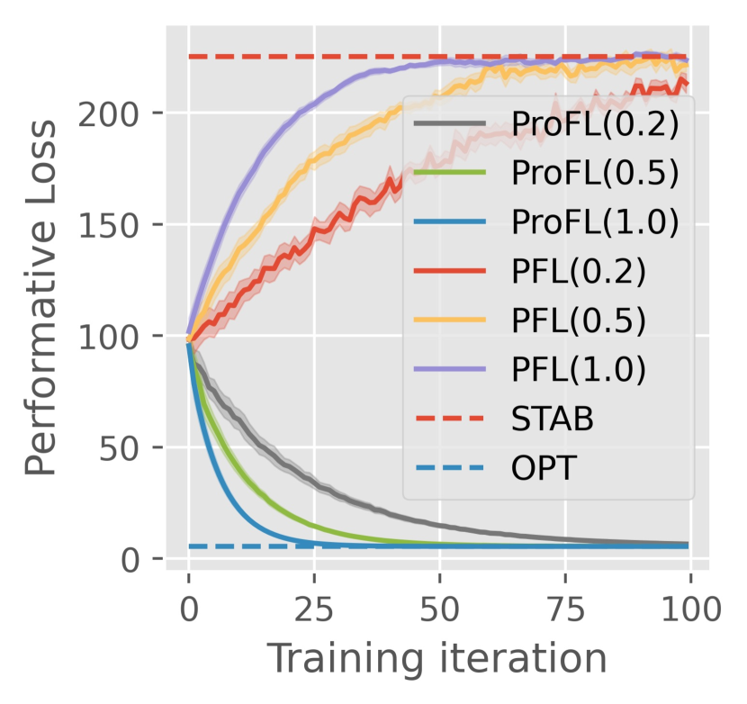
(a) Enrollment Fraction

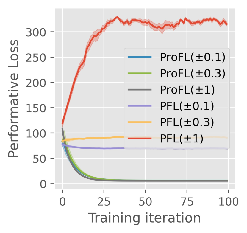
(b) Different Heterogeneity

Figure 3: Linear Regression Results with Different Enrollment Fractions and Heterogeneity

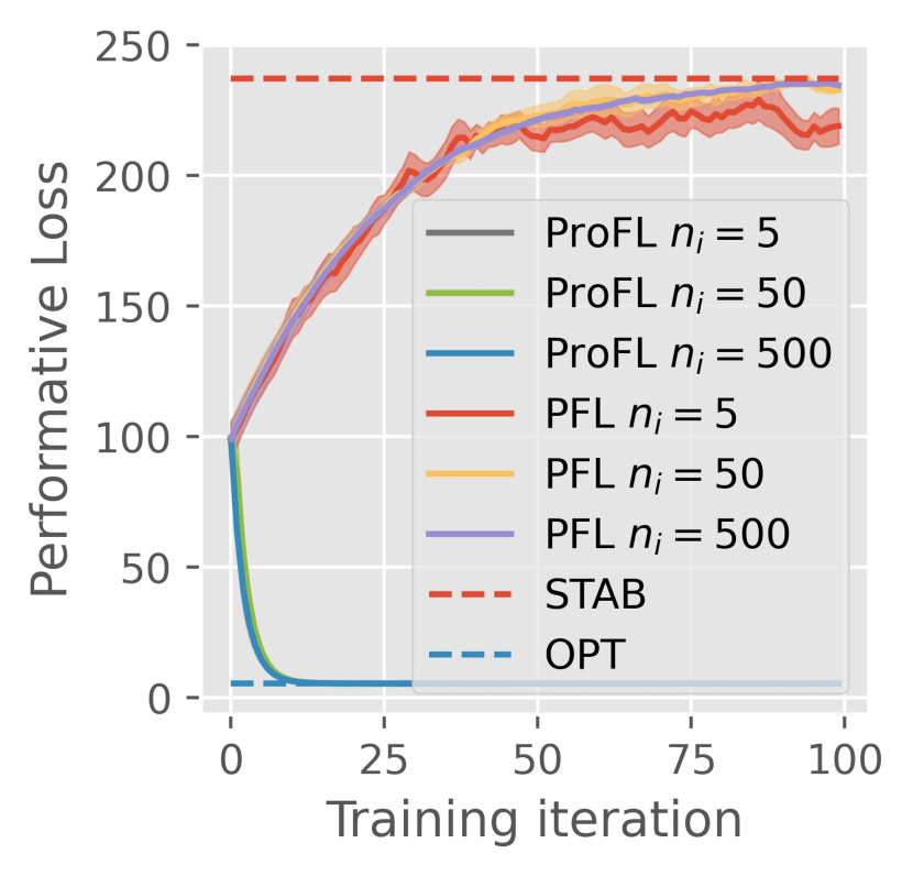
(a) Sample Size

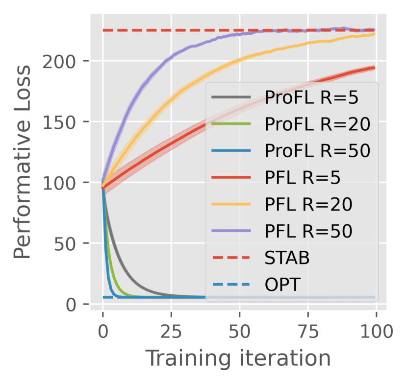
(b) Local Rounds $R$

Figure 4: Linear Regression Results with Different Sample Size and Local Rounds

In Fig. 4(a), the results show that both algorithms exhibit faster convergence rates with larger sample sizes. With a larger sample size, the results of PFL are closer to the performative stable point and exhibit fewer oscillations. However, PFL cannot converge to the performative optimal point, no matter how many samples are used. Fig. 4(b) demonstrates that a larger value of $R$ corresponds to faster convergence, reducing the communication time required in the FL system to reach convergence.

Fig. 5(a) shows the results of the case study pricing with dynamic contribution with 10 heterogeneous clients. The results indicate that, unlike PFL, which converges to $\theta^{\text{PS}}$, our algorithm converges to a solution, which is close to the performative optimal point. Fig. 5(b) shows the results of the case study regression with dynamic contribution with 10 heterogeneous clients. ProFL has faster convergence speed and less oscillation, although there is a gap between the results of both algorithms and the performative optimal point. The gap is a result of the non-linear $f_{i}(.)$, which has been discussed in more detail in the main paper.

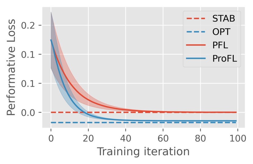
(a) Pricing

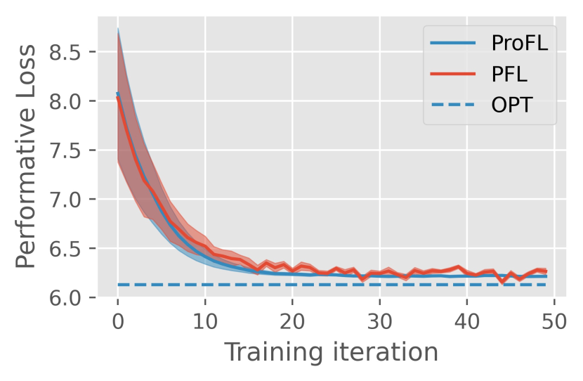
(b) Regression

Figure 5: Contribution Dynamics

D.2 Performance when ${\theta}^{\text{PO}}={\theta}^{\text{PS}}$

In this section, we introduce a special case where $\theta^{\text{PO}}=\theta^{\text{PS}}$. This special case can arise in both strategic and dynamic contribution settings. We present the results in Fig. 6, demonstrating that when $\theta^{\text{PO}}=\theta^{\text{PS}}$, both algorithms converge to the same point.

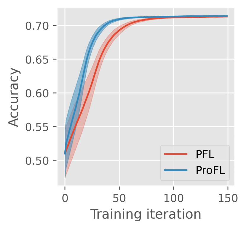
(a) Strategic Dynamic

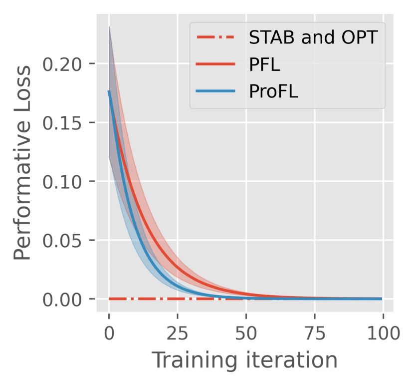
(b) Contribution Dynamic

Figure 6: Dynamics with ${\theta}^{\text{PO}}={\theta}^{\text{PS}}$

D.2.1 Performance without Model-dependent Shifts.

We also evaluate the algorithm when the data distribution does not change based on the model. In this case study, we use the Adult dataset for a binary classification task. Specifically, there are 10 homogeneous clients with $\gamma_{i,0}=\gamma_{i,1}=0$. We consider four features from the Adult dataset. When the data remains constant as the model is updated, both PFL and our algorithm reduce to FedAvg, and they converge to the same solution. This is illustrated in Fig. 6(a).

D.2.2 Performance when $\theta^{\text{PO}}=\theta^{\text{PS}}$ with Dynamic Contribution

Consider case study pricing with dynamic contribution with $K=2$ groups with different fixed distributions but a different one-dimensional fraction where $f_{i,1}(\theta)=0.5+0.5\theta$ and $f_{i,2}(\theta)=1-f_{i,1}(\theta)$. Under this special case, the performative stable and optimal points are identical, i.e., $\theta^{\text{PO}}=\theta^{\text{PS}}$. We can calculate $\theta^{\text{PO}}=\frac{a_{1}+a_{2}}{2(a_{1}-a_{2})}$ and $\theta^{\text{PS}}=\frac{a_{1}+a_{2}}{a_{1}-a_{2}}$. When $a_{1}+a_{2}=0$, $\theta^{\text{PO}}=\theta^{\text{PS}}$. In this case, we set $a_{1}=-a_{2}=0.5$. Fig. 6(b) illustrates the results for this specific case study, showing that both our algorithm and PFL converge to the same solution. However, our method exhibits faster convergence compared to PFL.

D.2.3 Figures of Table 2

The figures illustrating the experimental results from Table 2 in the main paper are shown in Fig. 7.

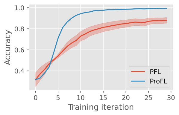
(a) Same Distributions

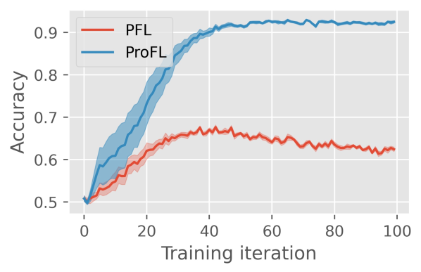
(b) Different Distributions

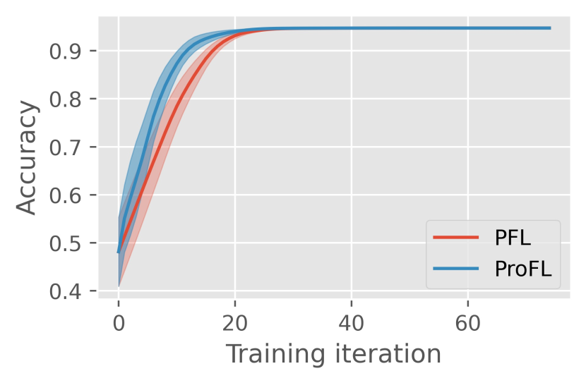
(c) Credit Dataset

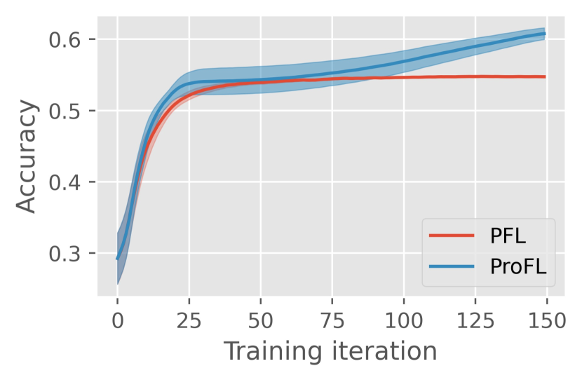
(d) Adult Dataset

Figure 7: Binary Classification on Synthetic and Realistic Dataset

Appendix E Training details

The experimental setup and parameter selections follow the methodology established in Izzo et al., (2021); Jin et al., (2024), ensuring consistency and comparability with existing results.

E.1 Realistic Data

• Adult data (Becker and Kohavi,, 1996) where the goal is to predict whether a person’s annual income exceeds $50K based on 14 features (e.g., age, years of education).

• Give Me Some Credit data (Credit Fusion,, 2011) which has 11 features (e.g., monthly income, debt ratio) and can be utilized to predict whether a person has experienced a 90-day past-due delinquency or worse.

E.2 Loss Functions and Ridge Penalty

We use ridge-regularized cross-entropy loss for all binary classification cases, and the ridge penalty is $0.01$. We use ridge-regularized squared loss for all regression cases, and the ridge penalty is $\frac{10}{3}$.

E.3 Random Seeds

In our experiments, which show the results of 10 trials, the random seeds used range from 0 to 9.

E.4 Parameters and Distributions

The experimental parameters are listed in Table 3, and the distribution $D_{i}(\cdot)$ for each experiment is detailed in Table 4. The corresponding case studies for the experiments are shown in Table 5.

Table 3: Parameters in the Experiments

Figure/Table	$\eta$	$R$	H	$n_{i}$	$\epsilon_{i}$
Table 1: PG	0.01	$-$	1	500	0
Table 1: ProFL	0.01	5	1	500	0
Table 2: Same $D_{i}$	0.03	10	500	500	0
Table 2: Different $D_{i}$	0.03	500	1	500	0
Table 2: Credit	0.01	5	1	5812	0
Table 2: Adult	0.03	5	1	2368	0
Figure 1a	0.001	5	25	500	0, 0.1,0.2,0.4
Figure 1b	0.0001	3	10	60	0
Figure 1c	0.001	5	100	1000	0
Figure 2a	0.001	5	20	50,500,5000	0
Figure 2b	0.01,0.03,0.001	5	20	2500	0
Figure 2c	0.001	5	4,20,100	500	0
Figure 3a	PFL:0.005 ProFL:0.001	5	0.2, 0.5, 1	500	0
Figure 3b	PFL:0.005 ProFL:0.001	5	1	500	0
Figure 3a	0.03	5	1	2368	0
Figure 3b	0.03	5	1	2368	0
Figure 4a	PFL:0.005 ProFL:0.001	5	1	5, 50, 500	0
Figure 4b	PFL:0.005 ProFL:0.001	5,20,50	1	500	0
Figure 5a	0.03	5	1	500	0
Figure 5b	0.001	5	1	500	0
Figure 6a	0.03	5	1	500	0
Figure 6b	0.03	5	1	500	0

Table 4: Data Distributions in the Experiments

Figure/Table	Distribution
Table 1: PG and ProFL	$\gamma_{i}\in[1.5-\alpha,1.5+\alpha]$, $\alpha\in\{0,0.25,0.5\}$
Table 2: Same $D_{i}$	$\gamma_{i,1}\in[2.8,3.2]$ and $X_{i}\sim\mathcal{N}(-1-\gamma_{i,1}\theta,0.25)$ for $Y=1$;
	$\gamma_{i,0}\in[0,0.04]$ and $X_{i}\sim\mathcal{N}(1-\gamma_{i,0}\theta,0.25)$ for $Y=0$.
Table 2: Different $D_{i}$	$\gamma_{i,1}\in[2.8,3.2]$, $X_{1}\sim\mathcal{N}(-1-\gamma_{i,1}\theta,0.25)$
	and $X_{2}\sim\mathcal{N}(-0.8-\gamma_{i,1}\theta,0.25)$ for $Y=1$;
	$\gamma_{i,0}\in[0,0.04]$ and $X_{i}\sim\mathcal{N}(1-\gamma_{i,0}\theta,0.25)$ for $Y=0$
Table 2: Credit	$\gamma_{i,1}=3$ and $\gamma_{i,0}=0.$ Give Me Some Credit datasetCredit Fusion, (2011)
Table 2: Adult	$\gamma_{i,1}\in[2.8,3.2]$ and $\gamma_{i,0}\in[0,0.004].$ Adult dataset (Becker and Kohavi,, 1996)
Figure 1a	$\mu_{0}\in[6,7]$, $\sigma=1$, $\gamma_{i}\in[1,3]$
Figure 1b,1c,2a-c	$\gamma_{i}\in[0.09,0.11]$
Figure 3a	$\gamma_{i}\in[1.5,1.8]$
Figure 3b	$\gamma_{i}\in[1.5-\alpha,1.5+\alpha]$, $\alpha\in\{0.1,0.3,1\}$
Figure 4a	$\gamma_{i}\in[1.5,1.8]$
Figure 4b	$\gamma_{i}\in[1.5,1.8]$
Figure 5a	$D_{i,1}\sim\mathcal{N}(0.5,0.25)$, $D_{i,2}\sim\mathcal{N}(-0.5,0.25)$ $f(\theta)=0.5+0.5\theta$
Figure 5b	$y=f_{i}(\theta)x+3(1-f_{i}(\theta))x+\varepsilon,\varepsilon\sim\mathcal{N}(0,4)$
Figure 6a	$\gamma_{i}=0.$ 10 homogeneous clients with Adult dataset
Figure 6b	$D_{i,1}\sim\mathcal{N}(0.5,0.25)$, $D_{i,2}\sim\mathcal{N}(-0.5,0.25)$

Table 5: Type of Case Study and Corresponding Figures or Tables

Figure/Table	Type of Case Study
Table 1:	house pricing regression
Table 2:	binary strategic classification
Figure 1a	pricing with dynamic demands
Figure 1b,1c,2a-c	pricing with dynamic contribution
Figure 3a,3b,4a,4b	house pricing regression
Figure 5a	pricing with dynamic contribution
Figure 5b	regression with dynamic contribution
Figure 6a	binary strategic classification
Figure 6b	pricing with dynamic contribution

References

• Becker and Kohavi, (1996) Becker, B. and Kohavi, R. (1996). Adult. UCI Machine Learning Repository. DOI: https://doi.org/10.24432/C5XW20.
• Bracale et al., (2024) Bracale, D., Maity, S., Banerjee, M., and Sun, Y. (2024). Learning the distribution map in reverse causal performative prediction.
• Briggs et al., (2020) Briggs, C., Fan, Z., and Andras, P. (2020). Federated learning with hierarchical clustering of local updates to improve training on non-iid data. In 2020 International Joint Conference on Neural Networks (IJCNN), pages 1–9. IEEE.
• Chen et al., (2024) Chen, Y., Tang, W., Ho, C.-J., and Liu, Y. (2024). Performative prediction with bandit feedback: Learning through reparameterization. In Salakhutdinov, R., Kolter, Z., Heller, K., Weller, A., Oliver, N., Scarlett, J., and Berkenkamp, F., editors, Proceedings of the 41st International Conference on Machine Learning, volume 235 of Proceedings of Machine Learning Research, pages 7298–7324. PMLR.
• Credit Fusion, (2011) Credit Fusion, W. C. (2011). Give me some credit.
• Dean and Morgenstern, (2022) Dean, S. and Morgenstern, J. (2022). Preference dynamics under personalized recommendations. In Proceedings of the 23rd ACM Conference on Economics and Computation, EC ’22, page 795–816. Association for Computing Machinery.
• Ensign et al., (2018) Ensign, D., Friedler, S. A., Neville, S., Scheidegger, C., and Venkatasubramanian, S. (2018). Runaway feedback loops in predictive policing. In Conference on fairness, accountability and transparency, pages 160–171. PMLR.
• Ghosh et al., (2020) Ghosh, A., Chung, J., Yin, D., and Ramchandran, K. (2020). An efficient framework for clustered federated learning. Advances in Neural Information Processing Systems, 33:19586–19597.
• Guo et al., (2023) Guo, Y., Lin, T., and Tang, X. (2023). Towards federated learning on time-evolving heterogeneous data.
• Hardt et al., (2016) Hardt, M., Megiddo, N., Papadimitriou, C., and Wootters, M. (2016). Strategic classification. In Proceedings of the 2016 ACM Conference on Innovations in Theoretical Computer Science, page 111–122.
• Huber, (1992) Huber, P. J. (1992). Robust estimation of a location parameter. In Breakthroughs in statistics: Methodology and distribution, pages 492–518. Springer.
• Izzo et al., (2021) Izzo, Z., Ying, L., and Zou, J. (2021). How to learn when data reacts to your model: Performative gradient descent. In Meila, M. and Zhang, T., editors, Proceedings of the 38th International Conference on Machine Learning, volume 139 of Proceedings of Machine Learning Research, pages 4641–4650. PMLR.
• Jiang and Lin, (2022) Jiang, L. and Lin, T. (2022). Test-time robust personalization for federated learning. In The Eleventh International Conference on Learning Representations.
• Jin et al., (2024) Jin, K., Yin, T., Chen, Z., Sun, Z., Zhang, X., Liu, Y., and Liu, M. (2024). Performative federated learning: A solution to model-dependent and heterogeneous distribution shifts. In Proceedings of the AAAI Conference on Artificial Intelligence, volume 38, pages 12938–12946.
• Li et al., (2021) Li, T., Hu, S., Beirami, A., and Smith, V. (2021). Ditto: Fair and robust federated learning through personalization. In Meila, M. and Zhang, T., editors, Proceedings of the 38th International Conference on Machine Learning, volume 139 of Proceedings of Machine Learning Research, pages 6357–6368. PMLR.
• (16) Li, T., Sahu, A. K., Talwalkar, A., and Smith, V. (2020a). Federated learning: Challenges, methods, and future directions. IEEE Signal Processing Magazine, 37(3):50–60.
• (17) Li, T., Sahu, A. K., Zaheer, M., Sanjabi, M., Talwalkar, A., and Smith, V. (2020b). Federated optimization in heterogeneous networks. In Dhillon, I., Papailiopoulos, D., and Sze, V., editors, Proceedings of Machine Learning and Systems, volume 2, pages 429–450.
• Ma et al., (2022) Ma, Y., Xie, Z., Wang, J., Chen, K., and Shou, L. (2022). Continual federated learning based on knowledge distillation. In Raedt, L. D., editor, Proceedings of the Thirty-First International Joint Conference on Artificial Intelligence, IJCAI-22, pages 2182–2188. International Joint Conferences on Artificial Intelligence Organization. Main Track.
• Mendler-Dünner et al., (2022) Mendler-Dünner, C., Ding, F., and Wang, Y. (2022). Anticipating performativity by predicting from predictions. In Koyejo, S., Mohamed, S., Agarwal, A., Belgrave, D., Cho, K., and Oh, A., editors, Advances in Neural Information Processing Systems, volume 35, pages 31171–31185. Curran Associates, Inc.
• Mendler-Dünner et al., (2020) Mendler-Dünner, C., Perdomo, J., Zrnic, T., and Hardt, M. (2020). Stochastic optimization for performative prediction. In Larochelle, H., Ranzato, M., Hadsell, R., Balcan, M., and Lin, H., editors, Advances in Neural Information Processing Systems, volume 33, pages 4929–4939. Curran Associates, Inc.
• Miller et al., (2021) Miller, J. P., Perdomo, J. C., and Zrnic, T. (2021). Outside the echo chamber: Optimizing the performative risk. In International Conference on Machine Learning, pages 7710–7720. PMLR.
• Nguyen et al., (2022) Nguyen, A. T., Torr, P., and Lim, S. N. (2022). Fedsr: A simple and effective domain generalization method for federated learning. In Koyejo, S., Mohamed, S., Agarwal, A., Belgrave, D., Cho, K., and Oh, A., editors, Advances in Neural Information Processing Systems, volume 35, pages 38831–38843. Curran Associates, Inc.
• Park et al., (2021) Park, T. J., Kumatani, K., and Dimitriadis, D. (2021). Tackling dynamics in federated incremental learning with variational embedding rehearsal. arXiv preprint arXiv:2110.09695.
• Perdomo et al., (2020) Perdomo, J., Zrnic, T., Mendler-Dünner, C., and Hardt, M. (2020). Performative prediction. In International Conference on Machine Learning, pages 7599–7609. PMLR.
• Polyak, (1964) Polyak, B. T. (1964). Some methods of speeding up the convergence of iteration methods. Ussr computational mathematics and mathematical physics, 4(5):1–17.
• Sattler et al., (2020) Sattler, F., Müller, K.-R., and Samek, W. (2020). Clustered federated learning: Model-agnostic distributed multitask optimization under privacy constraints. IEEE Transactions on Neural Networks and Learning Systems.
• Sattler et al., (2021) Sattler, F., Müller, K.-R., and Samek, W. (2021). Clustered federated learning: Model-agnostic distributed multitask optimization under privacy constraints. IEEE Transactions on Neural Networks and Learning Systems, 32(8):3710–3722.
• Shan et al., (2023) Shan, J.-W., Zhao, P., and Zhou, Z.-H. (2023). Beyond performative prediction: Open-environment learning with presence of corruptions. In International Conference on Artificial Intelligence and Statistics, pages 7981–7998. PMLR.
• Somerstep et al., (2024) Somerstep, S., Sun, Y., and Ritov, Y. (2024). Learning in reverse causal strategic environments with ramifications on two sided markets. ArXiv, abs/2404.13240.
• Tan et al., (2023) Tan, A. Z., Yu, H., Cui, L., and Yang, Q. (2023). Towards personalized federated learning. IEEE Transactions on Neural Networks and Learning Systems, 34(12):9587–9603.
• Wang and Ji, (2022) Wang, S. and Ji, M. (2022). A unified analysis of federated learning with arbitrary client participation. Advances in Neural Information Processing Systems, 35:19124–19137.
• Xie and Zhang, (2024) Xie, T. and Zhang, X. (2024). Non-linear welfare-aware strategic learning.
• Zhang et al., (2022) Zhang, X., Khalili, M. M., Jin, K., Naghizadeh, P., and Liu, M. (2022). Fairness interventions as (Dis)Incentives for strategic manipulation. In Proceedings of the 39th International Conference on Machine Learning, pages 26239–26264.
• Zhao, (2022) Zhao, Y. (2022). Optimizing the performative risk under weak convexity assumptions. OPT2022: 14th Annual Workshop on Optimization for Machine Learning, abs/2209.00771.
• Zheng et al., (2022) Zheng, Q., Zhang, A., and Grover, A. (2022). Online decision transformer. In Chaudhuri, K., Jegelka, S., Song, L., Szepesvari, C., Niu, G., and Sabato, S., editors, Proceedings of the 39th International Conference on Machine Learning, volume 162 of Proceedings of Machine Learning Research, pages 27042–27059. PMLR.
• Zhu et al., (2021) Zhu, C., Xu, Z., Chen, M., Konečnỳ, J., Hard, A., and Goldstein, T. (2021). Diurnal or nocturnal? federated learning of multi-branch networks from periodically shifting distributions. In International Conference on Learning Representations.