MOFFlow: Flow Matching for Structure Prediction of Metal-Organic Frameworks

Abstract

Metal-organic frameworks (MOFs) are a class of crystalline materials with promising applications in many areas such as carbon capture and drug delivery. In this work, we introduce MOFFlow, the first deep generative model tailored for MOF structure prediction. Existing approaches, including ab initio calculations and even deep generative models, struggle with the complexity of MOF structures due to the large number of atoms in the unit cells. To address this limitation, we propose a novel Riemannian flow matching framework that reduces the dimensionality of the problem by treating the metal nodes and organic linkers as rigid bodies, capitalizing on the inherent modularity of MOFs. By operating in the $SE(3)$ space, MOFFlow effectively captures the roto-translational dynamics of these rigid components in a scalable way. Our experiment demonstrates that MOFFlow accurately predicts MOF structures containing several hundred atoms, significantly outperforming conventional methods and state-of-the-art machine learning baselines while being much faster.

1 Introduction

Metal-organic frameworks (MOFs) are a class of crystalline materials that have recently received significant attention for their broad range of applications, including gas storage (Li et al., 2018), gas separations (Qian et al., 2020), catalysis (Lee et al., 2009), drug delivery (Horcajada et al., 2012), sensing (Kreno et al., 2012), and water purification (Haque et al., 2011). They are particularly valued for their permanent porosity, high stability, and remarkable versatility due to their tunable structures. In particular, MOFs are tunable by adjusting their building blocks, i.e., metal nodes and organic linkers, to modify pore size, shape, and chemical characteristics to suit specific applications (Wang et al., 2013). Consequently, there is a growing interest in developing automated approaches to designing and simulating MOFs using computational algorithms.

Crystal structure prediction (CSP) is a task of central importance for automated MOF design and simulation. The importance of this task lies in the fact that the important functions of MOFs, such as pore size, surface area, and stability, are directly dependent on the crystal structure. The conventional approach to general CSP is based heavily on ab initio calculations using density functional theory (DFT; Kohn & Sham, 1965), often combined with optimization algorithms such as random search (Pickard & Needs, 2011) and Bayesian optimization (Yamashita et al., 2018) to iteratively explore the energy landscape. However, the reliance on DFT for such computations can be computationally expensive, especially for large and complex systems such as MOFs.

Deep generative models are promising solutions to accelerate the prediction of the MOF structure. Especially, diffusion models (Ho et al., 2020) and flow-based models (Lipman et al., 2023) have shown success in similar molecular structure prediction problems, e.g., small molecules (Xu et al., 2022; Jing et al., 2022), folded proteins (Jing et al., 2024; Lin et al., 2023), protein-ligand complex (Corso et al., 2023), and general crystals without the building block constraint (Gebauer et al., 2022; Xie et al., 2022; Jiao et al., 2024a; Miller et al., 2024). These models iteratively denoise the random structure using neural networks that act similar to force fields guiding atom positions toward a minimum energy configuration.

Contribution. In this work, we introduce MOFFlow, the first deep generative model tailored for MOF structure prediction. MOFFlow leverages the modular nature of MOFs, which can be decomposed into metal nodes and organic linkers (Figures 1, LABEL: and 2). This decomposition enables us to design a generative model that predicts the roto-translation of these building blocks to match the ground truth structure. To achieve this, based on Riemannian flow matching (Chen & Lipman, 2024), we propose a new framework that generates rotations, translations, and lattice structure of the building blocks. We design the underlying neural network as a composition of building block encoder parameterized by an equivariant graph neural network based on a new attention module for encoding roto-translations and lattice parameters of the MOF.

We note that our method competes with existing deep-generative models (Gebauer et al., 2022; Xie et al., 2022; Jiao et al., 2024a; Miller et al., 2024) for general CSP that encompass MOFs as special members. However, our method is specialized for MOF structure prediction by exploiting the domain knowledge that the local structures of the MOF building blocks are shared across different MOF structures. This is particularly useful for reducing the large search space of MOF structures; We consider MOFs up to 2,200 atoms per unit cell (Boyd et al., 2019), whereas crystals for general CSP consist of up to 52 atoms per unit cell (Jain et al., 2013; Jiao et al., 2024a). In fact, as confirmed in our experiments, the recent deep generative model (Jiao et al., 2024a) for general CSP fails to scale to the large system size of MOFs. This also aligns with how torsional diffusion (Jing et al., 2022) improved over existing molecular conformer generation algorithms (Xu et al., 2021; 2022) by eliminating the redundant degree of freedom.

We benchmark our algorithm with the MOF dataset compiled by Boyd et al. (2019), consisting of 324,426 structures. We compare with conventional and deep learning-based algorithms for crystal structure prediction. Notably, MOFFlow achieves a match rate of $31.69\%$ on unseen MOF structures, whereas existing methods, despite being more computationally expensive, barely match any. We also demonstrate that MOFFlow captures key MOF properties and scales efficiently to structures containing hundreds of atoms.

Figure 1: Overview of MOFFlow. MOFFlow is a continuous normalizing flow that exploits the modular nature of MOFs by modeling the building blocks (i.e., metal nodes and organic linkers) as rigid bodies. It learns the vector fields for rotation ($\bm{q}$), translation ($\bm{\tau}$), and the lattice ($\bm{\ell}$) that assembles the building blocks into a complete MOF structure.

Figure 2: Inference trajectory of MOFFlow. Visualization of the inference trajectory of MOFFlow from $t=0$ to $t=1$, showing the progressive assembly of building blocks. We wrap building block centroids inside the lattice for visual clarity.

2 Related work

Crystal structure prediction (CSP). Traditional approaches to CSP rely on density functional theory (DFT) to identify energetically stable structures. To generate candidate structures, heuristic techniques such as random sampling (Pickard & Needs, 2011) and simple substitution rules (Wang et al., 2021) have been employed, alongside more sophisticated optimization algorithms such as Bayesian optimization (Yamashita et al., 2018), genetic algorithms (Yamashita et al., 2022), and particle swarm optimization (Wang et al., 2010). To address the computational burden with DFT calculations, many studies used machine learning as surrogates for energy evaluation (Jacobsen et al., 2018; Podryabinkin et al., 2019; Cheng et al., 2022).

Recently, deep generative models have emerged as a promising alternative to optimization-based methods (Court et al., 2020; Hoffmann et al., 2019; Noh et al., 2019; Yang et al., 2021; Hu et al., 2020; 2021; Kim et al., 2020; Ren et al., 2022). Notably, Jiao et al. (2024a) proposes an equivariant diffusion-based model to capture the periodic $E(3)$-invariance of crystal structure distributions, while Lin et al. (2024) and Jiao et al. (2024b) additionally consider lattice permutations and space group constraints, respectively. Miller et al. (2024) uses Riemannian flow matching to generate high-quality samples with fewer integration steps. However, these methods face significant challenges in predicting the MOFs structures, which often consist of hundreds of atoms per unit cell.

MOF structure prediction. Unlike general CSP, where a variety of algorithms have been developed, MOF structure prediction remains a significant challenge. Conventional MOF structure prediction methods heavily rely on predefined topologies to connect MOF building blocks (Marleny Rodriguez-Albelo et al., 2009; Wu & Jiang, 2024), restricting the discovery of structures with new topologies. To address this limitation, Darby et al. (2020) proposes to combine ab initio random structure searching (AIRSS; Pickard & Needs, 2011) with the Wyckoff alignment of molecules (WAM) method; however, the reliance on AIRSS makes it computationally expensive. We also note that a recent work (Fu et al., 2023) considered a related, yet different problem of MOF generation based on a deep generative model which does not include the structure generation.

Flow matching. Flow matching is a simulation-free approach for training continuous normalizing flows, originally introduced by Lipman et al. (2023). Since its introduction, various extensions have been proposed, such as generalization to Riemannian manifolds (Chen & Lipman, 2024) and efficiency improvements through optimal transport (Tong et al., 2024; Pooladian et al., 2023). Due to its flexibility and computational efficiency, flow matching has made notable progress in several related domains, including protein generation (Yim et al., 2023a; b; 2024; Bose et al., 2024), molecular conformation generation (Song et al., 2024), and CSP (Miller et al., 2024).

3 Preliminaries

3.1 Representation of MOF structures

MOF representation. The 3D crystal structure of a MOF can be represented with the periodic arrangement of the smallest repeating unit called the unit cell. A unit cell containing $N$ atoms can be represented with the tuple $\mathcal{S}=(\bm{X},\bm{a},\bm{\ell})$ where $\bm{X}=[x_{n}]_{n=1}^{N}\in\mathbb{R}^{N\times 3}$ is the atom coordinates, $\bm{a}=[a_{n}]_{n=1}^{N}\in\mathcal{A}^{N}$ is the atom types with $\mathcal{A}$ denoting the set of possible elements, and $\bm{\ell}=(a,b,c,\alpha,\beta,\gamma)\in\mathbb{R}_{+}^{3}\times[0,180]^{3}$ is the lattice parameter that describes the periodicity of the structure (Miller et al., 2024; Luo et al., 2024). In particular, the lattice parameter $\bm{\ell}$ can be transformed into a standard lattice matrix $L\in\mathbb{R}^{3\times 3}$, which defines the infinite crystal structure:

$$\{(a_{n}^{\prime},x_{n}^{\prime})|a_{n}^{\prime}=a_{n},x_{n}^{\prime}=x_{n}+Lk,k\in\mathbb{Z}^{3}\}$$ (1)

where $k=(k_{1},k_{2},k_{3})$ is the set of integers representing the periodic translation of the unit cell.

Block-wise representation of MOFs. Here we introduce the blockwise representation of MOFs that decompose a given unit cell into constituent building blocks, i.e., the metal nodes and organic linkers. The blockwise representation is a tuple $\mathcal{S}=(\mathcal{B},\bm{q},\bm{\tau},\bm{\ell})$ where $\mathcal{B}=\{\mathcal{C}_{m}\}_{m=1}^{M}$ corresponds to $M$ building blocks and $\bm{q}=[q_{m}]_{m=1}^{M},\bm{\tau}=[\tau_{m}]_{m=1}^{M}$ corresponds to set of $M$ building block roto-translations $(q_{m},\tau_{m})\in SE(3)$ . Moreover, each block $\mathcal{C}_{m}=(\bm{a}_{m},\bm{Y}_{m})$ has $N_{m}$ atoms with atom types $\bm{a}_{m}=[a_{n}]_{n=1}^{N_{m}}\in\mathcal{A}^{N_{m}}$ and local coordinates $\bm{Y}_{m}=[y_{n}]_{n=1}^{N_{m}}\in\mathbb{R}^{N_{m}\times 3}$. Our main assumption is that the building blocks can be composed by the roto-translations to form the MOF structure, i.e., the atomwise representation $(\bm{X},\bm{a},\bm{\ell})$ can be expressed by the blockwise representation $(\bm{q},\bm{\tau},\mathcal{B},\bm{\ell})$:

$$\bm{X}=\operatorname{Concat}(\bm{X}_{1},\ldots,\bm{X}_{M}),\quad\bm{X}_{m}=(q_{m},\tau_{m})\cdot\bm{Y}_{m},$$

where $\bm{X}_{m}$ is the result of the roto-translated local coordinate represented by group action $\cdot$. We express the global coordinate $\bm{X}$ as the concatenation $\bm{X}_{m}$’s without loss of generality.

3.2 Flow matching on Riemannian manifolds

Flow matching is a method to train continuous normalizing flow (CNF; Chen et al., 2018) without expensive ordinary differential equation (ODE) simulations (Lipman et al., 2023). Here, we introduce the flow matching generalized to Riemannian manifolds (Chen & Lipman, 2024).

CNF in Riemannian manifold. We consider a smooth and connected Riemann manifold $\mathcal{M}$ with metric $g$ where each point $x\in\mathcal{M}$ is associated with tangent space $\mathcal{T}_{x}\mathcal{M}$ and inner product $\langle\cdot,\cdot\rangle_{g}$. We consider learning a CNF $\phi_{t}:\mathcal{M}\rightarrow\mathcal{M}$ defined with the ODE $\frac{d}{dt}\phi_{t}(x)=u_{t}(\phi_{t}(x))$ where $\phi_{0}(x)=x$ and $u_{t}(x)\in\mathcal{T}_{x}\mathcal{M}$ is the time-dependent smooth vector field. The vector field $u_{t}(x)$ transforms a prior distribution $p_{0}$ to $p_{t}$ according to the following push-forward equation:

$$p_{t}(x)=[\phi_{t}]_{*}p_{0}(x)-p_{0}(\phi_{t}^{-1}(x))\exp\bigg{(}{-\int_{0}^{t}\nabla\cdot u_{t}(x_{s})ds}\bigg{)},\qquad t\in[0,1],$$ (2)

where $\nabla\cdot$ is the divergence operator and $x_{s}=\phi_{s}(\phi_{t}^{-1}(x))$.

Conditional flow matching on Riemannian manifold. The goal of CNF is to learn a vector field $u_{t}(\cdot)$ that transforms a simple prior distribution $p_{0}$ so that $p_{1}$ closely approximates some target distribution $q$. Given a vector field $u_{t}(\cdot)$ and the corresponding probability paths $\{p_{t}\}_{t\in[0,1]}$, one can train a neural network $v_{t}(x;\theta)$ with the flow matching objective:

$$\mathcal{L}_{\text{FM}}(\theta)=\mathbb{E}_{t,p_{t}(x)}[\lVert v_{t}(x;\theta)-u_{t}(x)\rVert_{g}^{2}],$$ (3)

where $t\sim\mathcal{U}[0,1]$, $x\sim p_{t}(x)$, and $\lVert\cdot\rVert_{g}$ is the norm induced by the metric $g$. However, the flow matching objective lacks analytic form of $u_{t}(x)$ that transforms the prior $p_{0}$ into the target $q$. The key insight of conditional flow matching objective is to instead learn a conditional vector field $u_{t}(x|x_{1})$ for a data point $x_{1}$ defined as follows:

$$\mathcal{L}_{\text{CFM}}(\theta)=\mathbb{E}_{t,p_{1}(x),p_{t}(x|x_{1})}[\lVert v_{t}(x;\theta)-u_{t}(x|x_{1})\rVert_{g}^{2}],$$ (4)

where we let $p_{0}(x|x_{1})=p_{0}(x)$ and $p_{1}(x|x_{1})\approx\delta(x-x_{1})$ with $\delta(\cdot)$ being the Dirac distribution. The key idea of conditional flow matching is that one can derive the conditional vector field $u_{t}(x|x_{1})$ that marginalizes over data points $x_{1}\sim q$ accordingly to induce the vector field $u_{t}(x)$ transforming the prior $p_{0}$ into the desired distribution $q$. To construct $u_{t}(x|x_{1})$, Chen & Lipman (2024) proposes defining conditional flow $x_{t}=\phi_{t}(x_{0}|x_{1})$ from the geodesic path (minimum length curve) connecting two points $x_{0},x_{1}\in\mathcal{M}$ by $x_{t}=\exp_{x_{0}}(t\log_{x_{0}}(x_{1}))$ for $t\in[0,1]$, where $\exp_{x}$ and $\log_{x}$ are the exponential and logarithmic map at point $x\in\mathcal{M}$, respectively. Then the desired conditional vector field can be derived as the time derivative, i.e., $u(x_{t}|x_{1})=\frac{d}{dt}\phi_{t}(x_{0}|x_{1})$.

At optimum, $v_{\theta}$ generates $p_{t}^{\theta}=p_{t}$ with starting point $p_{0}^{\theta}=p_{0}$ and end point $p_{1}^{\theta}=p_{1}$. At inference, we sample from the prior $p_{0}^{\theta}$ and propagate $t$ from $0$ to $1$ using one of the existing ODE solvers. Note that each training step is faster than the methods based on adjoint sensitivity (Chen et al., 2018) since conditional flow matching does not require solving the ODE defined by the neural network.

4 Methods

In this section, we introduce MOFFlow, a novel approach for MOF structure prediction based on the rigid-body roto-translation of building blocks to express the global atomic coordinates. To this end, using the Riemannian flow matching framework, we learn a CNF $p_{\theta}(\bm{q},\bm{\tau},\bm{\ell}|\mathcal{B})$ that predicts the blockwise roto-translations and the lattice parameter from the given building blocks. Compared to conventional CSP approaches defined on atomic coordinates (Jiao et al., 2024a; b; Lin et al., 2024; Miller et al., 2024), MOFFlow enjoys the reduced search space, i.e., the dimensionality of blockwise roto-translation and the atomic coordinates are $6M$ and $3N$, respectively ($6M\ll 3N$).

4.1 Construction of local coordinates

To incorporate the MOF symmetries, we devise a scheme to consistently define the local coordinate $\bm{Y}$ regardless of the initial pose of the building block. Given a building block $\mathcal{C}=(\bm{a},\bm{Y})$, our goal is to define a global-to-local function $f:\mathcal{A}\times\mathbb{R}^{N\times 3}\rightarrow{}\mathbb{R}^{N\times 3}$ that defines a consistent local coordinate system; that is, the function should satisfy

$$f(\bm{a},\bm{X}Q^{\top}+1_{N}t^{\top})=f(\bm{a},\bm{X}),\quad\forall Q\in SO(3),t\in\mathbb{R}^{3}.$$ (5)

where $\bm{X}$ is a random conformation of the building block. We can then define $\bm{Y}=f(\bm{a},\bm{X})$. Such property can be satisfied by a composition of (1) translation by subtracting the centroid and (2) rotation by aligning with the principal component analysis (PCA) axes:

$$f(a,\bm{X})=C(\bm{X})\mathcal{R}(\bm{a},C(\bm{X})),\quad C(\bm{X})=\bm{X}-1_{N}\left(\frac{1}{N}\sum_{n=1}^{N}x_{n}^{\top}\right).$$ (6)

Here, $C(\bm{X})$ denotes subtraction of the centroid and $\mathcal{R}(\bm{a},\bm{X})$ denotes rotation to align the building block with the PCA axes whose sign is fixed by a reference vector, following Gao & Günnemann (2022). See Appendix D for more details.

4.2 Flow matching for MOF structure prediction

In this section, we present our approach to training the generative model $p_{\theta}(\bm{q},\bm{\tau},\bm{\ell}|\mathcal{B})$ using the flow matching framework. We first explain how our method ensures $SE(3)$-invariance and introduce a metric for independent treatment of the components $\bm{q}$, $\bm{\tau}$, and $\bm{\ell}$. Next, we outline the key elements for flow matching – i.e., the definition of priors, conditional flows, and the training objective.

To preserve crystal symmetries, we design the framework such that the generative model is invariant to rotation, translation, and permutation of atoms and building blocks. Rotation invariance is guaranteed by using the rotation-invariant lattice parameter representation and canonicalizing the atomic coordinates based on the standard lattice matrix (Miller et al., 2024; Luo et al., 2024). Translation invariance is achieved by operating on the mean-free system where the building blocks are centered at the origin – i.e., $\frac{1}{M}\sum_{m=1}^{M}\tau_{m}=0$. This is the only way to ensure translation invariance on $SE(3)^{M}$ as no $\mathbb{R}^{3}$ invariant probability measure exists (Yim et al., 2023b). Permutation invariance is addressed using equivariant graph neural networks (Satorras et al., 2021) and Transformers (Vaswani, 2017) as the backbone.

Metric for $SE(3)$. Following Yim et al. (2023b), we treat $SO(3)$ and $\mathbb{R}^{3}$ independently by defining an additive metric on $SE(3)$ as

$$\langle(q,\tau),(q^{\prime},\tau^{\prime})\rangle_{SE(3)}=\langle q,q^{\prime}\rangle_{SO(3)}+\langle\tau,\tau^{\prime}\rangle_{\mathbb{R}^{3}}.$$ (7)

Here, $\langle q,q^{\prime}\rangle_{SO(3)}$ and $\langle\tau,\tau^{\prime}\rangle_{\mathbb{R}^{3}}$ are inner products defined as $\langle q,q^{\prime}\rangle_{SO(3)}=\text{tr}(qq^{\prime\top})/2$ and $\langle\tau,\tau^{\prime}\rangle_{\mathbb{R}^{3}}=\tau^{\top}\tau^{\prime}$ for $q,q^{\prime}\in\mathfrak{so}(3)$ with $\mathfrak{so}(3)$ denoting the Lie algebra of $SO(3)$ and $\tau,\tau^{\prime}\in\mathbb{R}^{3}$.

Priors. For each rotation $q$ and translation $\tau$, the prior are chosen as the uniform distribution on $SO(3)$ and standard normal distribution on $\mathbb{R}^{3}$, respectively. For the lattice parameter $\ell$, we follow Miller et al. (2024) and use log-normal and uniform distributions. Specifically, for the lengths, we let $p_{0}(a,b,c)=\prod_{\lambda\in\{a,b,c\}}\operatorname{LogNormal}(\lambda;\mu_{\lambda},\sigma_{\lambda})$ where the parameters are learned with the maximum-likelihood objective (Appendix C). For the angles, we use Niggli reduction (Grosse-Kunstleve et al., 2004) to constrain the distribution to the range $p_{0}(\alpha,\beta,\gamma)=\mathcal{U}(60,120)$.

Conditional flows. Following Chen & Lipman (2024), we train the model to match the conditional flow defined along the geodesic path of the Riemannian manifold:

$$q^{(t)}=\exp_{q^{(0)}}(t\log_{q^{(0)}}(q^{(1)})),\quad\tau^{(t)}=(1-t)\tau^{(0)}+t\tau^{(1)},\quad\bm{\ell}^{(t)}=(1-t)\bm{\ell}^{(0)}+t\bm{\ell}^{(1)}.$$ (8)

Here, $\exp_{q}$ is the exponential map and $\log_{q}$ is the logarithmic map at point $q$. From this definition, the conditional vector fields are derived from the time derivatives:

$$u_{t}(q^{(t)}|q^{(1)})=\frac{\log_{q^{(t)}}(q^{(1)})}{1-t},\quad u_{t}(\tau^{(t)}|\tau^{(1)})=\frac{\tau^{(1)}-\tau^{(t)}}{1-t},\quad u_{t}(\bm{\ell}^{(t)}|\bm{\ell}^{(1)})=\frac{\bm{\ell}^{(1)}-\bm{\ell}^{(t)}}{1-t}.$$ (9)

Training objective. Instead of directly modeling the vector fields, we leverage a closed-form expression that enables re-parameterization of the network to predict the clean data $\bm{q}_{1},\bm{\tau}_{1},\bm{\ell}_{1}$ from the intermediate MOF structure $\mathcal{S}^{(t)}=(\bm{q}_{t},\bm{\tau}_{t},\bm{\ell}_{t},\mathcal{B})$. To achieve this, we train a neural network to approximate the clean data, expressed as $(\bm{\hat{q}}_{1},\bm{\hat{\tau}}_{1},\hat{\bm{\ell}}_{1})=\mathcal{F}(\mathcal{S}^{(t)};\theta)$ with regression on clean data:

$$\mathcal{L}(\theta)= \mathbb{E}_{\mathcal{M}^{(1)}\sim\mathcal{D}}\mathbb{E}_{t\in\mathcal{U}(0,1)}\big{[}\lambda_{1}\lVert\bm{\hat{q}}_{1}-\bm{q}_{1}\rVert_{SO(3)}+\lambda_{2}\lVert\bm{\hat{\tau}}_{1}-\bm{\tau}_{1}\rVert_{\mathbb{R}^{3}}+\lambda_{3}\lVert\hat{\bm{\ell}}_{1}-\bm{\ell}_{1}\rVert_{\mathbb{R}^{3}}\big{]},$$ (10)

where $\mathcal{D}$ is the dataset, $\mathcal{U}(0,1)$ is the uniform distribution defined on an interval $[0,1]$, and $\lambda_{1},\lambda_{2},\lambda_{3}$ are loss coefficients (see Appendix C).

4.3 Model Architecture

(a) Atom-level update layer

(b) Block-level update modules

Figure 3: Overview of our neural network architecture. (3(a)) The atom-level update layers encode building block representations into embeddings at the atomic resolution. (3(b)) The block-level modules iteratively update the roto-translations $(\bm{q},\bm{\tau})$, block features $\bm{H}$, pairwise features $\bm{Z}$, and lattice parameter $\bm{\ell}$ to predict the clean data $(\hat{\bm{q}}_{1},\hat{\bm{\tau}}_{1},\hat{\bm{\ell}}_{1})$.

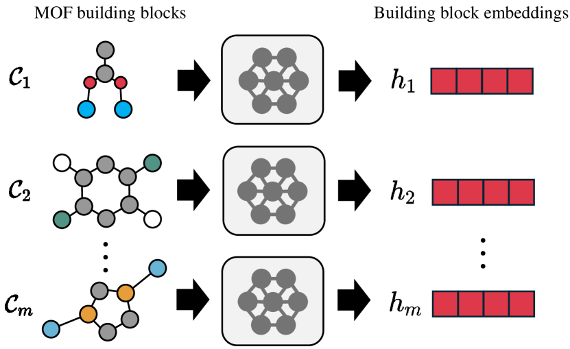
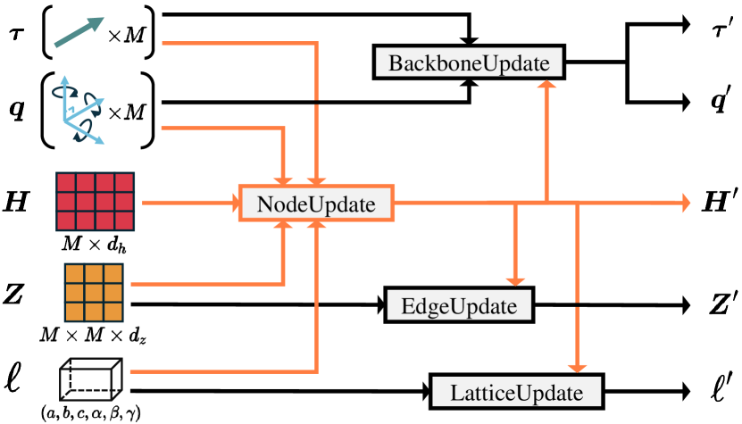
Here, we describe the architecture of our neural network $\mathcal{F}(\mathcal{S}^{(t)};\theta)$ used to predict clean data $(\bm{{q}}_{1},\bm{{\tau}}_{1},{\ell}_{1})$. We have two key modules: (1) the atom-level update layers to obtain the building block embeddings from atomic resolution, and (2) the building block-level update layers that aggregate and update information over MOF on building block resolution and predict $\bm{{q}}_{1}$, $\bm{{\tau}}_{1}$, and ${\ell}_{1}$ from the final building block embeddings. In what follows, we describe each module one-by-one.

Atom-level update layers. The atom-level update layers (Figure 3(a)) process the building block representation $\mathcal{C}_{m}=(\bm{a}_{m},\bm{Y}_{m})$ for $m=1,\ldots,M$ to output the building block embedding $h_{m}$. They are graph neural networks operating on an undirected graph $\mathcal{G}_{m}=(\mathcal{V}_{m},\mathcal{E}_{m})$ constructed from adding an edge between a pair of atoms within the cutoff distance of $5\text{\r{A}}$. It initializes the atom-wise features $\{v_{k}:k=1,\ldots,N_{m}\}$ from atom types and the edge features $\{e_{k,k^{\prime}}:\{k,k^{\prime}\}\in\mathcal{E}\}$ from atomic distances. Each layer updates the atom features $\{v_{k}:k=1,\ldots,N_{m}\}$ as follows:

$$v_{k}^{\prime}=v_{k}+\phi_{v}\bigg{(}v_{k},\sum_{k^{\prime}\in\mathcal{N}(k)}\phi_{e}\left(v_{k},v_{k^{\prime}},e_{k,k^{\prime}}\right)\bigg{)},$$ (11)

where $\{v_{k}^{\prime}:k=1,\ldots,N_{m}\}$ is the set of updated atom features, $\mathcal{N}(k)$ denotes the neighbor of atom $k$ in the graph $\mathcal{G}_{m}$, and $\phi_{v}$, $\phi_{e}$ are multi-layer perceptrons (MLPs). Finally, the building block embedding $h_{m}$ is obtained from applying mean pooling of the node embeddings at the last layer followed by concatenation with sinusoidal time embedding of $t$ (Vaswani, 2017) and an MLP.

Block-level update modules. Each layer of the update module (Figure 3(b)) iteratively updates its prediction of $(\bm{q},\bm{\tau})\in{SE(3)^{M}}$ and $\ell$ along with the block features $\bm{H}=[h_{m}]_{m=1}^{M}\in\mathbb{R}^{M\times d_{h}}$ and the pairwise features $\bm{Z}=[z_{mm^{\prime}}]_{m,m^{\prime}=1}^{M}\in\mathbb{R}^{M\times M\times d_{z}}$. The predictions are initialized by the intermediate flow matching output $\bm{q}_{t},\bm{\tau}_{t},\ell_{t}$, the node features are initialized from the atom-level update layers, and the edge features are initialized as follows:

$$z_{mm^{\prime}}=\phi_{z}(h_{m},h_{m^{\prime}},\operatorname{dgram}({\lVert\tau_{m}-\tau_{m^{\prime}}\rVert}_{2}),\operatorname{dgram}({\lVert\hat{\tau}_{m}-\hat{\tau}_{m^{\prime}}\rVert}_{2})),$$ (12)

where $\operatorname{dgram}$ computes a distogram binning the pairwise distance into equally spaced intervals between $0\text{\r{A}}$ and $20\text{\r{A}}$. Finally, the block-level update module is defined as follows:

$$\bm{H}^{\prime} =\operatorname{NodeUpdate}(\bm{H},\bm{Z},\bm{q},\bm{\tau},\ell),\quad\bm{Z}^{\prime}=\operatorname{EdgeUpdate}(\bm{Z},\bm{H}^{\prime}),$$ (13)

$$(\bm{q}^{\prime},\bm{\tau}^{\prime}) =\operatorname{BackboneUpdate}(\bm{q},\bm{\tau},\bm{H}^{\prime}),\quad\ell^{\prime}=\operatorname{LatticeUpdate}(\ell,\bm{H}^{\prime}),$$ (14)

where $\bm{q}^{\prime},\bm{\tau}^{\prime},\bm{H}^{\prime},\bm{Z}^{\prime},\ell^{\prime}$ are the updated predictions and the features. Importantly, $\operatorname{NodeUpdate}$ operator consists of the newly designed $\operatorname{MOFAttention}$ module followed by pre-layer normalization $\operatorname{Transformers}$ (Xiong et al., 2020) and MLP with residual connections in between. The $\operatorname{EdgeUpdate}$, $\operatorname{BackboneUpdate}$ modules are implemented as in Yim et al. (2023b) and $\operatorname{LatticeUpdate}$ is identity function for the lattice parameter except for the last layer. At the final layer, the lattice parameter is predicted from mean pooling of the block features followed by an MLP. Complete details of each update module are in Appendix E.

In particular, our $\operatorname{MOFAttention}$ module is modification of the invariant point attention module proposed by Jumper et al. (2021) for processing protein frames. Our modification consists of adding the lattice parameter as input and simplification by removing the edge aggregation information. In particular, the lattice parameter is embedded using a linear layer and added as an offset for the attention matrix between the building blocks. We provide more details in Algorithm 1.

Algorithm 1 $\operatorname{MOFAttention}$ module

Input: Node features $\bm{H}=[h_{m}]_{m=1}^{M}$, edge features $\bm{Z}=[z_{mm^{\prime}}]_{m,m^{\prime}=1}^{M}$, rotations $\bm{q}=[q_{m}]_{m=1}^{M}$, translations $\bm{\tau}=[\tau_{m}]_{m=1}^{M}$, lattice parameter $\bm{\ell}$, number of building blocks $M$, number of heads $N_{h}$, number of non-rotating channels $N_{c}$, and number of rotating channels $N_{r}$.
Output: Updated node features $\bm{H}^{\prime}=[h_{m}^{\prime}]_{m=1}^{M}$.

1:for $h\in\{1,\ldots,N_{h}\}$ do

2:     for $m\in\{1,\ldots,M\}$ do $\triangleright$ Query, key, values.

3:         $q_{mh},k_{mh},v_{mh}=\text{Linear}_{h}(h_{m})$. $\triangleright$ $q_{mh},k_{mh},v_{mh}\in\mathbb{R}^{N_{c}}$.

4:         $\tilde{q}_{mhp},\tilde{k}_{mhp},\tilde{v}_{mhp}=(q_{m},\tau_{m})\cdot\text{Linear}_{h}(h_{m})$. $\triangleright$ $\tilde{q}_{mh},\tilde{k}_{mh},\tilde{v}_{mh}\in\mathbb{R}^{3N_{r}}.$

5:     end for

6:     $l_{h}=\text{Linear}_{h}(\ell)$. $\triangleright$ Lattice structure encoding $l_{h}\in\mathbb{R}$.

7:     $b_{mm^{\prime}h}=\text{Linear}_{h}(z_{mm^{\prime}})$ for $m,m^{\prime}\in\{1,\ldots,M\}$. $\triangleright$ Attention bias $b_{mm^{\prime}h}\in\mathbb{R}$.

8:     $\gamma_{h}=\text{SoftPlus}(\text{Linear}_{h}(1))$.$\triangleright$ Learnable coefficient $\gamma_{h}\in\mathbb{R}$

9:     $C_{1}=\frac{1}{\sqrt{N_{c}}}$ and $C_{2}=\sqrt{\frac{2}{9N_{r}}}$. $\triangleright$ Coefficients $C_{1},C_{2}\in\mathbb{R}$.

10:     for $m,m^{\prime}\in\{1,\ldots,M\}$ do $\triangleright$ Attention $a_{mm^{\prime}h}\in\mathbb{R}$.

11:         $a_{mm^{\prime}h}=\text{SoftMax}\left(\frac{1}{2}\left(C_{1}q_{mh}^{\top}k_{m^{\prime}h}+b_{mm^{\prime}h}+l_{h}-\frac{C_{2}\gamma_{h}}{2}\lVert{\tilde{q}}_{mhp}-{\tilde{k}}_{m^{\prime}hp}\rVert^{2}\right)\right)$.

12:     end for

13:     ${o}_{mh}=\sum_{m^{\prime}}a_{mm^{\prime}h}{v}_{m^{\prime}h}$ and $\tilde{o}_{mh}=\sum_{m^{\prime}}a_{mm^{\prime}h}\tilde{v}_{m^{\prime}h}$ for $m\in\{1,\ldots,M\}$. $\triangleright$ Aggregate.

14:end for

15:$h_{m}^{\prime}=\text{Linear}(\text{Concat}_{h,p}(o_{mh},\tilde{o}_{mhp},\ell))$ for $m\in\{1,\ldots,M\}$ $\triangleright$ Update the node features.

5 Experiments

The goal of our experiments is to address two questions. Accuracy: How does the structure prediction accuracy of MOFFlow compare to other approaches? Scalability: How does the performance of MOFFlow vary with an increasing number of atoms and building blocks?

To address the first question, Section 5.1 compares the structure prediction accuracy of MOFFlow against both conventional and deep learning-based methods. Furthermore, Section 5.2 evaluates whether MOFFlow can capture essential MOF properties, further validating the accuracy of its predictions. The second question is answered in Section 5.3, where we analyze the performance of MOFFlow with increasing system size. Additionally in Section 5.4, we compare MOFFlow to the self-assembly algorithm (Fu et al., 2023) by integrating it with our approach.

5.1 Structure prediction

Dataset. We use the dataset from Boyd et al. (2019), containing 324,426 MOF structures. Following Fu et al. (2023), we apply the metal-oxo decomposition of MOFid (Bucior et al., 2019) to decompose each structure into building blocks. After filtering structures with fewer than 200 blocks, we split the data into train/valid/test sets in an 8:1:1 ratio. Full data statistics are in Appendix A.

Baselines. We compare our model with two types of methods: optimization-based algorithms and deep learning-based methods. For traditional approach, we use CrySPY (Yamashita et al., 2021) to implement the random search (RS) and evolutionary algorithm (EA). For deep learning, we benchmark against DiffCSP (Jiao et al., 2024a), which generates structures based on atom types. MOF-specific methods are excluded due to lack of public availability.

Metrics. We evaluate using match rate (MR) and root mean square error (RMSE). We compare the samples to the ground truth using StructureMatcher class of pymatgen (Ong et al., 2013). Two sets of threshold for $\operatorname{stol}$, $\operatorname{ltol}$, and $\operatorname{angle\_tol}$ are used: $(0.5,0.3,10.0)$ in alignment with the general CSP literature (Jiao et al., 2024a; b; Chen & Lipman, 2024) and $(1.0,0.3,10.0)$ to account for the difficulty of predicting large structures. MR is the proportion of matched structures and RMSE is the root mean squared displacement normalized by the average free length per atom. We also measure the time required to generate $k$ samples, averaged across all test sets.

Implementation. Both RS and EA use CHGnet (Deng et al., 2023) for structure optimization. We generate 20 samples for RS, while EA starts with 5 initial, 20 populations, and 20 generations. Due to the high computational cost for large crystals, generating more samples was not feasible. For DiffCSP, we follow the hyperparameters from Jiao et al. (2024a) and train for 200 epochs. Our method uses an AdamW optimizer (Loshchilov, 2017) with a learning rate of $10^{-4}$ and $\beta=(0.9,0.98)$. We use a maximum batch size of 160 and run inference with 50 integration steps. We generate $1$ and $5$ samples for DiffCSP and our method. Implementation details are in Appendix C.

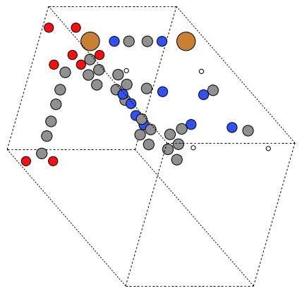
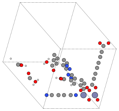
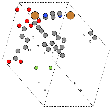
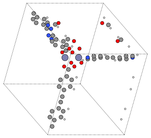
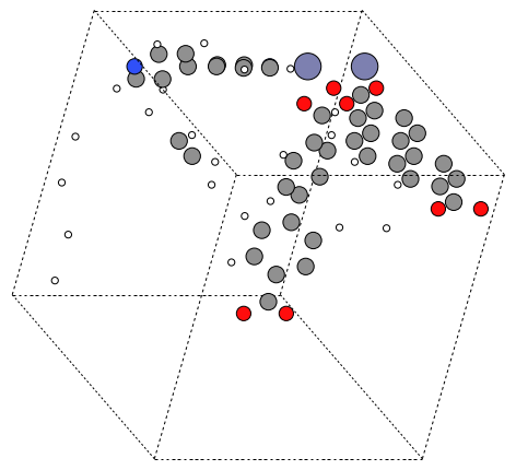
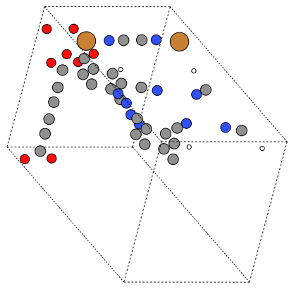
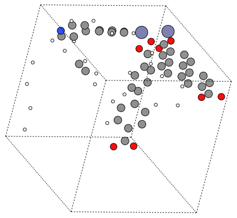
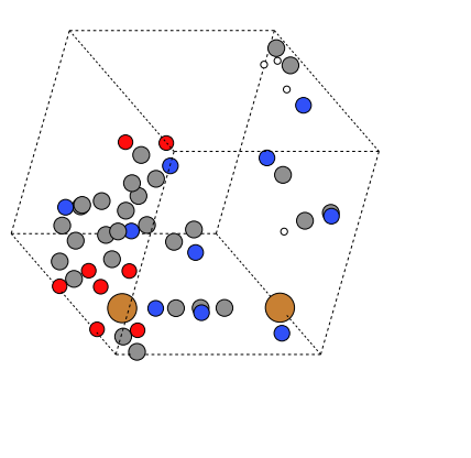
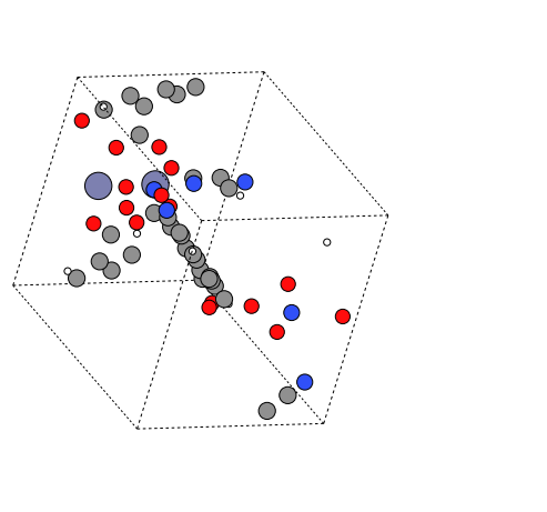
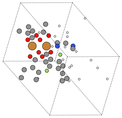
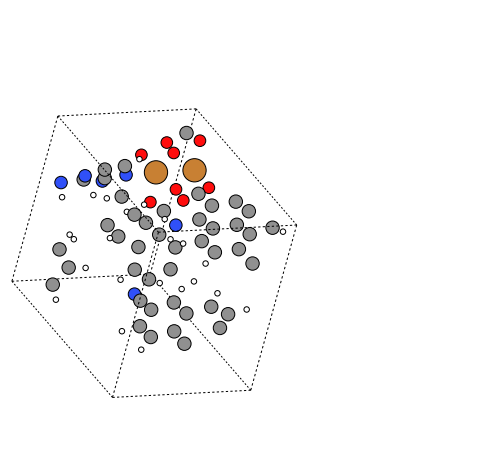
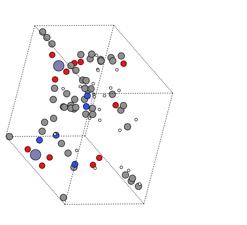
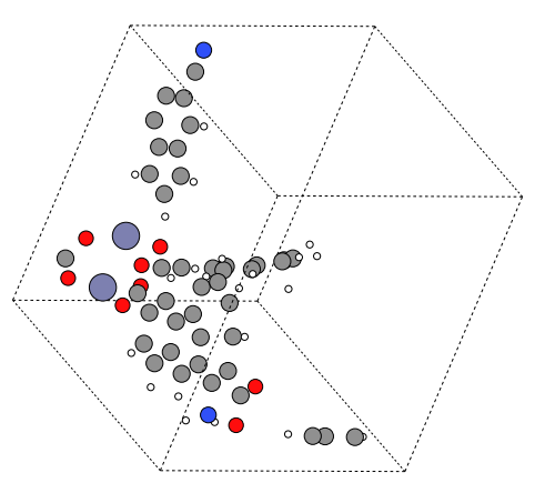
Results. Table 1 presents the results, where MOFFlow outperforms all baselines. Optimization-based methods yield zero MR, highlighting the challenge of using the conventional atom-based approach for large systems. DiffCSP also performs poorly, underscoring the need to incorporate building block information in MOF structure prediction. While we achieve a 100% MR at $\operatorname{stol}=1.0$, this threshold is too lenient for practical application; however, we include it for multi-level comparison. Visualizations comparing samples from MOFFlow and DiffCSP are shown in Figure 4.

Table 1: Structure prediction accuracy. We evaluate structure prediction performance across optimization-based methods (RS, EA), a deep generative model (DiffCSP), and our method, MOFFlow. Due to computational constraints, RS and EA were tested on 100 and 15 samples, respectively, while DiffCSP and MOFFlow were evaluated on the full test set of 30,880 structures. MR refers to the match rate, and RMSE to the root mean squared error; - indicates no match. $\operatorname{stol}$ represents the site tolerance for matching criteria. The reported time is the average per structure. MOFFlow outperforms all baselines in MR, RMSE, and generation time.

	# of samples	$\operatorname{stol}=0.5$		$\operatorname{stol}=1.0$		Avg. time (s)$\downarrow$
		MR (%) $\uparrow$	RMSE $\downarrow$	MR (%) $\uparrow$	RMSE $\downarrow$
RS (Yamashita et al., 2021)	20	00.00	-	00.00	-	0332
EA (Yamashita et al., 2021)	20	00.00	-	00.00	-	1959
DiffCSP (Jiao et al., 2024a)	1	00.09	0.3961	23.12	0.8294	05.37
	5	00.34	0.3848	38.94	0.7937	26.85
MOFFlow (Ours)	1	31.69	0.2820	87.46	0.5183	01.94
	5	44.75	0.2694	100.0	0.4645	05.69

	Cu2 H4 C28 N10 O8	Zn2 H8 C32 N6 O16	Cu2 H18 C26 N2 O8 F2	Cu2 H24 C44 N6 O8	Zn2 H24 C48 N6 O12	Zn8 H46 C72 O27
Ground Truth
Ours
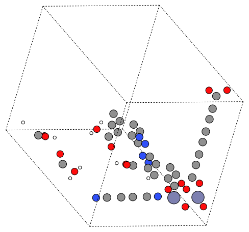
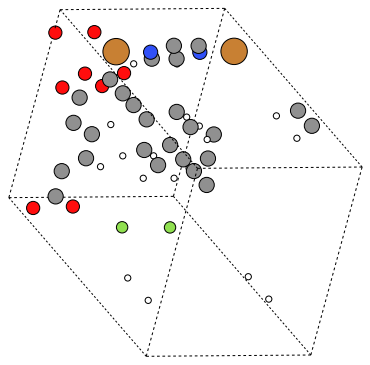
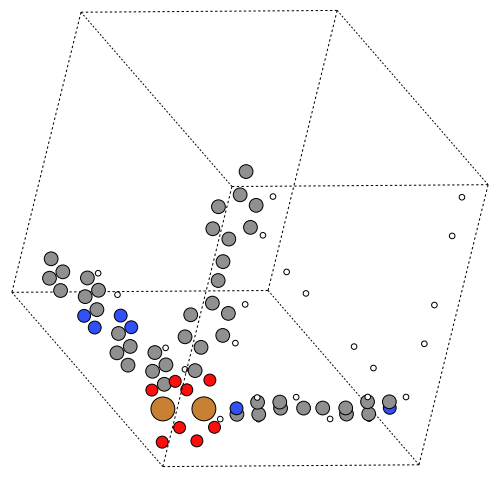
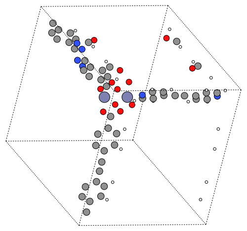
DiffCSP

Figure 4: Visualization of the predicted MOF structures. We select structures from the 20 candidates with the lowest RMSE. The lattice is scaled to represent the relative size between generated structures. Our model accurately generates high-quality MOF structure predictions with accurate atomic positions and lattice configuration.

Figure 5: Property distributions. We compare the distributions of key MOF properties for ground-truth, MOFFlow, and DiffCSP. The distributions are histograms smoothed by kernel density estimation. Property units are displayed in the top-right corner of each plot. MOFFlow (red) closely aligns with the ground-truth distribution (blue), while DiffCSP (yellow) shows noticeable deviations. These results highlight that MOFFlow’s ability to accurately capture essential MOF properties.

5.2 Property evaluation

In this section, we demonstrate that MOFFlow accurately captures the key properties of ground-truth MOF structures, offering a more detailed assessment of prediction quality beyond match rate and RMSE. These properties are crucial for various MOF applications, such as gas storage and catalysis. Specifically, we evaluate volumetric surface area (VSA), gravimetric surface area (GSA), largest cavity diameter (LCD), pore limiting diameter (PLD), void fraction (VF), density (DST), accessible volume (AV), and unit cell volume (UCV). Definitions and the details of each property are provided in Appendix B.

Table 2: Property evaluation. Average RMSE computed between the ground-truth and generated structures for MOFFlow and DiffCSP. MOFFlow achieve lower error across all properties, demonstrating its ability to generate high-quality samples that accurately capture MOF properties.

	RMSE $\downarrow$
	MOFFlow	DiffCSP
VSA ($m^{2}/cm^{3}$)	264.5	0796.9
GSA ($m^{2}/g$)	331.6	1561.9
AV ($\AA^{3}$)	530.5	3010.2
UCV ($\AA^{3}$)	569.5	3183.4
VF	0.0285	0.2167
PLD ($\AA$)	1.0616	4.0581
LCD ($\AA$)	1.1083	4.5180
DST ($g/cm^{3}$)	0.0442	0.3711

For comparison, we use DiffCSP as a representative of general CSP approaches. We exclude optimization-based baselines as they did not yield meaningful results. For each test structure from Section 5.1, we generate a single sample and compute the relevant properties using Zeo++ (Willems et al., 2012). We do not filter our samples with the match criteria from Section 5.1. We use 50 integration steps for our model and measure performance with RMSE.

Results. Table 2 shows that MOFFlow consistently yields lower errors than DiffCSP across all evaluated properties. This demonstrates its ability to produce high-quality predictions while preserving essential MOF characteristics. Additionally, Figure 5 visualizes the property distributions, where our model closely reproduces the ground-truth distributions and captures key characteristics. In contrast, DiffCSP frequently reduces volumetric surface area and void fraction to zero, highlighting the limitations of conventional approaches in accurately modeling MOF properties.

5.3 Scalability evaluation

Here, we demonstrate that MOFFlow enables structure prediction for large systems, which is a challenge for general CSP methods. To evaluate how performance scales with system size, we analyze match rates as a function of the number of atoms and building blocks. We compare our results with DiffCSP as the representative of the general CSP approach. We generate single samples for each test structure and use thresholds $(1.0,0.3,10.0)$ for visibility.

Figure 6: Scalability evaluation. (left) Match rate comparison between MOFFlow and DiffCSP by atom count. MOFFlow preserves high match rates across all bins, while DiffCSP drops sharply beyond 200 atoms. (right) Match rate of MOFFlow by building block count, with our method performing well even for complex structures with many blocks. These results highlight the scalability of our approach.

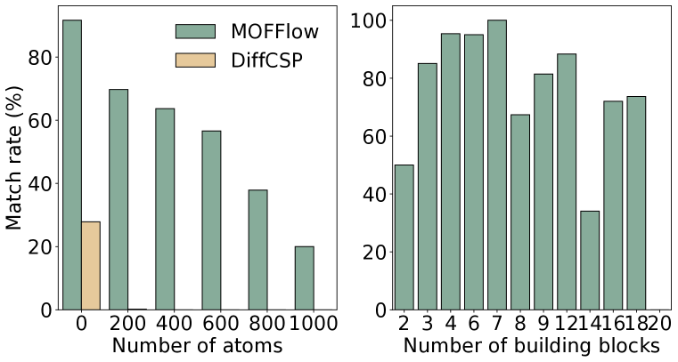
Results. Figure 6 presents our findings, with the $x$-axis representing the number of atoms, binned in ranges of $(t,t+200]$. The final bin includes all atom counts beyond the last range, without an upper limit. MOFFlow consistently outperforms DiffCSP across all atom ranges. While our approach shows only gradual performance degradation as atom count increases, DiffCSP suffers a sharp decline for systems with more than 100 atoms and fails to predict structures with over 200 atoms. In contrast, our method maintains a high match rate even for structures exceeding 1,000 atoms per unit cell, highlighting the effectiveness of leveraging building block information for MOF structure prediction. Additionally, Figure 6 shows how our match rate scales with the number of building blocks. The results show minimal performance degradation, demonstrating that our model effectively handles larger numbers of building blocks and efficiently scales to large crystal structures.

5.4 Comparison to self-assembly algorithm

Table 3: Comparison with self-assembly (SA) algorithm. Since SA can only predict rotations, we provide translations and lattice predicted by MOFFlow for fair comparison. MOFFlow alone achieves higher accuracy and faster inference times than SA.

	MR (%) $\uparrow$	RMSE $\downarrow$	Time (s) $\downarrow$
SA	30.04	0.3084	4.75
Ours	31.69	0.2820	1.94

To make our evaluation more comprehensive, we also consider the self-assembly algorithm used by Fu et al. (2023) as a baseline, although the performance is not directly comparable. The self-assembly (SA) algorithm is an optimization-based method that predicts the rotation $\bm{q}$ by maximizing the overlap between building block connection points. Since the algorithm requires $\bm{\tau}$, $\bm{\ell}$, and $\mathcal{C}$ as input, it is not directly applicable for structure prediction on its own. Therefore, we conduct an ablation by combining the self-assembly algorithm with our predicted values of $\bm{\tau}$ and $\bm{\ell}$. We note that the self-assembly algorithm defines the centroid as the center of mass of the connection points, and we account for this offset in our implementation.

Results. Table 3 shows that MOFFlow alone outperforms the combination with the self-assembly algorithm, indicating that learning the building block orientations leads to more accurate MOF structure predictions than heuristic-based overlap optimization. Additionally, our method offers faster inference, further demonstrating its efficiency compared to optimization-based approaches.

6 Conclusion

We propose MOFFlow, a building block-based approach for predicting the structure of metal-organic frameworks (MOFs). Our approach significantly outperforms general crystal structure prediction algorithms – in both quality and efficiency – that fail to account for the modularity of MOFs. Additionally, MOFFlow is scalable, successfully predicting structures composed of up to thousands of atoms.

Reproducibility

We describe experimental details and hyperparameters in Appendix C. We provide our codes and model checkpoint in https://anonymous.4open.science/r/MOFFlow-3547.

Ethic Statement

Our framework targets to advance porous material discovery, which is deeply related to carbon capturing, catalysis design, and drug discovery. We believe our work can improve the quality of human life by assisting in resolving global warming and drug design. However, they should notice the caution due to the misuse in developing hazardous materials or products that may be harmful for specific usage.

Appendix A Data statistics

In this section, we present the data statistics to represent the characteristics of the MOF dataset. We consider the MOF dataset from Boyd et al. (2019) and the dataset is generated by the MOF-generating algorithms based on the topology from graph theory. The dataset is distributed on the materialscloud. As mention in Section 5.1, we uses filtered strucutures with fewer than 200 blocks. The dataset is divided into train, valid and test in an 8:1:1 ratio. The statistic of data splits are represented in the Tables 4, LABEL:, 5, LABEL: and 6.

Property (number of samples $=247,066$)	Min	Mean	Max
number of species / atoms	3 / 20	5.3 / 151.5	8 / 2208
working capacity (vacuum) [$10^{-3}$mol/g]	-0.2618	0.4177	4.8355
working capacity (temperature) [$10^{-3}$mol/g]	-0.2712	0.2843	4.4044
volume [$\AA^{3}$]	534.5	5496.7	193341.7
density [atoms/$\AA^{3}$]	0.0737	0.7746	4.0966
lattice $a,b,c$ [$\AA$]	6.13 / 8.27 / 8.56	13.81 / 16.47 / 20.39	57.83 / 57.80 / 61.62
lattice $\alpha,\beta,\gamma$ [∘]	59.76 / 59.99 / 59.97	91.08 / 91.05 / 90.75	120.29 / 120.01 / 120.02

Table 4: The statistics of the train split of MOF dataset.

Property (number of samples $=30,883$)	Min	Mean	Max
number of species / atoms	3 / 16	5.3 / 152.4	8 / 2256
working capacity (vacuum) [$10^{-3}$mol/g]	-0.2510	0.4163	5.1152
working capacity (temperature) [$10^{-3}$mol/g]	-0.1210	0.2834	4.4589
volume [$\AA^{3}$]	534.5	5538.1	118597.4
density [atoms/$\AA^{3}$]	0.11	0.77	4.33
lattice $a,b,c$ [$\AA$]	6.86 / 8.43 / 8.57	13.85 / 16.53 / 20.39	48.29 / 55.11 / 60.97
lattice $\alpha,\beta,\gamma$ [∘]	59.98 / 59.99 / 59.99	91.08 / 91.00 / 90.73	120.11 / 120.01 / 120.02

Table 5: The statistics of the valid split of MOF dataset.

Property (number of samples $=30,880)$	Min	Mean	Max
number of species / atoms	3 / 22	5.3 / 149.3	8 / 2368
working capacity (vacuum) [$10^{-3}$mol/g]	-0.1999	0.4193	4.6545
working capacity (temperature) [$10^{-3}$mol/g]	-0.1318	0.2858	3.9931
volume [$\AA^{3}$]	536.4	5401.1	124062.6
density [atoms/$\AA^{3}$]	0.108	0.777	4.074
lattice $a,b,c$ [$\AA$]	6.86 / 8.34 / 8.56	13.74 / 16.39 / 20.26	49.86 / 49.88 / 60.95
lattice $\alpha,\beta,\gamma$ [∘]	59.91 / 60.00 / 59.99	91.00 / 90.98 / 90.76	120.16 / 120.01 / 120.01

Table 6: The statistics of the test split of MOF dataset.

Appendix B Glossary

Structural properties. In this section, we introduce the structural properties we measured. These properties were calculated using the Zeo++ software package developed by Willems et al. (2012). Zeo++ provides high-throughput geometry-based analysis of crystalline porous materials, calculating critical features such as pore diameters, surface area, and accessible volume, all of which are essential for evaluating material performance in applications such as gas storage and catalysis.

Specifically, we calculated properties including volumetric surface area (VSA), the surface area per unit volume; gravimetric surface area (GSA), which represents the surface area per unit mass; the largest cavity diameter (LCD), which represents the diameter of the largest spherical cavity within the material; the pore limiting diameter (PLD), defined as the smallest passage through which molecules must pass to access internal voids; the void fraction (VF) (Martin & Haranczyk, 2014), which is the ratio of total pore volume in the structure to the total cell volume; the density (DST), which refers to the mass per unit volume of the material; the accessible volume (AV), indicating the volume available to the center of a given probe molecule within the pores; and the unit cell volume (UCV), representing the total volume of the repeating unit cell in the crystal structure. These parameters provide critical insights into the MOF’s porosity, surface area, and ability to store and transport gases, and recent study shows the correlation with these properties with the bulk material (Krishnapriyan et al., 2020).

Appendix C Implementation details

Training details. We employ the $\operatorname{TimestepBatch}$ algorithm (Yim et al., 2023b) to efficiently construct batches. This method generates a batch by applying multiple noise levels $t\in[0,1]$ to a single data instance, ensuring uniform batch size. To manage memory constraints, we cap the batch size with $N^{2}$, where $N$ is the number of atoms. The model is trained on eight 24GB NVIDIA RTX 3090 GPUs over 15 epochs, taking approximately 7 days.

Hyperparameters. Table 7 and Table 8 shows model and training hyperparameters for MOFFlow, respectively. In practice, we generate $q$, $k$, and $v$ from $h$ independently, allowing each to have a distinct dimension. The non-rotating channels are represented as a tuple, with $qk$ and $v$ specified in that order. We set the log-normal distribution parameters for lattice lengths to $\mu=(2.55,2.75,2.96)$ and $\sigma=(0.3739,0.3011,0.3126)$, computed from the training data with the closed-form maximum likelihood estimation.

Baselines. For DiffCSP (Jiao et al., 2024a), we change the edge construction method from original fully connected to a radius graph with a cutoff of 5Å since a fully connected graph is not feasible for large-size crystals like MOFs. We use batch size 8 to cope with memory constraints. Any other options followed the default hyperparameter of the DiffCSP. We trained 200 epochs, taking approximately 7 days until convergence on a 24GB NVIDIA RTX 3090 GPU.

For random search (RS) and evolutionary algorithms (EA) for structure prediction, we considered CrySPY (Yamashita et al., 2021) software and deep-learning based structure optimizer (Deng et al., 2023). We set the symmetry-based search for RS and constructed 20 structures per sample. Also, we set the EA for 5 initial RS and ran a maximum of 20 generations with 10 crossovers, 4 permutations, 2 strains, and 2 elites for 20 populations. We considered the tournament-selection function for 4 tournament sizes. We used energy-based optimization for RS and EA, since there exists no publicly opened software for MOF crystal structure prediction.

Code. Our implementation is built upon https://github.com/microsoft/protein-frame-flow, https://github.com/microsoft/MOFDiff, https://github.com/gcorso/DiffDock, and https://github.com/vgsatorras/egnn. We appreciate the authors (Yim et al., 2023a; b; 2024; Fu et al., 2023; Corso et al., 2023; Satorras et al., 2021) for their contributions.

Table 7: Model hyperparameters of MOFFlow

Hyperparameter	Value
Atom-level node dimension	64
Atom-level edge dimension	64
Atom-level cutoff radius	5
Atom-level maximum atoms	100
Atom-level update layers	4
Block-level node dimension	256
Block-level edge dimension	128
Block-level time dimension	128
Block-level update layers	6
$\operatorname{MOFAttention}$ number of heads	24
$\operatorname{MOFAttention}$ rotating channels	256
$\operatorname{MOFAttention}$ non-rotating channels	(8, 12)

Table 8: Training hyperparameters of MOFFlow

Hyperparameter	Value
loss coefficient $\lambda_{1}$ ($\bm{q}$)	1.0
loss coefficient $\lambda_{2}$ ($\bm{\tau}$)	2.0
loss coefficient $\lambda_{3}$ ($\bm{\ell}$)	0.1
batch size	160
maximum $N^{2}$	1,600,000
optimizer	AdamW
initial learning rate	0.0001
betas	(0.9, 0.98)
learning rate scheduler	ReduceLROnPlateau
learning rate patience	30 epochs
learning rate factor	0.6

Appendix D Defining local coordinates of building blocks

Following, Gao & Günnemann (2022), we use principle component analysis (PCA) as our backbone since it is $SO(3)$-equivariant up to a sign. Specifically, if we denote $\text{PCA}(X)=[e_{1},e_{2},e_{3}]$, in the order of decreasing eigenvalues, $\forall Q\in SO(3)$,

$$\operatorname{PCA}(\bm{X}Q^{\top})=c\odot Q\\ \operatorname{PCA}(\bm{X}),\quad c\in\{-1,+1\}^{3}$$

that is, the sign is not preserved upon rotation. To define a consistent direction, Gao & Günnemann (2022) suggests the use of an equivariant vector function $v(\bm{a},\bm{X})$ as

$$\tilde{e}_{i}=\begin{cases}e_{i},&\text{if $v(\bm{a},\bm{X})^{\top}e_{i}\geq 0$}\\ -e_{i},&\text{otherwise}.\end{cases}$$ (15)

Then, the final equivariant axes is defined as $\mathcal{R}=[\tilde{e}_{1},\tilde{e}_{2},\tilde{e}_{3}]$ where $\tilde{e}_{3}=\tilde{e}_{1}\times\tilde{e}_{2}$.

However, we find that this definition is insufficient for our application where some building blocks are 2-dimensional exhibit symmetry with respect to the origin and thus have $v(\bm{a},\bm{X})=0$. For such cases, we define

$$v_{\text{sym}}(\bm{X})=\operatorname*{arg\,min}_{x\in\bm{X}}\{{\lVert x\rVert}^{2}|x\neq 0\}$$

– i.e., the vector from the centroid to the closest atom. Since the building blocks are symmetric, $f$ still fulfills Equation 5 up to permutation, which is handled by GNN and Transformers.

Appendix E Model architecture

Here, we provide the details of the $\operatorname{NodeUpdate}$, $\operatorname{EdgeUpdate}$, and $\operatorname{BackboneUpdate}$ modules. Our implementation follows Yim et al. (2023b); Jumper et al. (2021), with the exception of the $\operatorname{MOFAttention}$ module and the $\operatorname{Transformers}$, where we use a pre-layer normalized version (Xiong et al., 2020). Each module is introduced with our notation. The function $R(a,b,c,d)$ in Algorithm 4 is defined as

$$R(a,b,c,d)=\left(\begin{smallmatrix}(a^{n})^{2}+(b^{n})^{2}-(c^{n})^{2}-(d^{n})^{2}&2b^{n}c^{n}-2a^{n}d^{n}&2b^{n}d^{n}+2a^{n}c^{n}\\ 2b^{n}c^{n}+2a^{n}d^{n}&(a^{n})^{2}-(b^{n})^{2}+(c^{n})^{2}-(d^{n})^{2}&2c^{n}d^{n}-2a^{n}b^{n}\\ 2b^{n}d^{n}-2a^{n}c^{n}&2c^{n}d^{n}-2a^{n}b^{n}&(a^{n})^{2}-(b^{n})^{2}-(c^{n})^{2}+(d^{n})^{2}\end{smallmatrix}\right).$$ (16)

Algorithm 2 $\operatorname{NodeUpdate}$ Module

Input: $(\bm{q},\bm{\tau},\bm{H},\bm{Z},\bm{\ell})$
Output: $\bm{H}^{\prime}$

1:$\tilde{\bm{H}}\leftarrow{}\operatorname{LayerNorm}(\operatorname{MOFAttention}(\bm{q},\bm{\tau},\bm{H},\bm{Z},\bm{\ell})+\bm{H})$

2:$\tilde{\bm{H}}\leftarrow{}\operatorname{Concat}(\bm{\tilde{H}},\operatorname{Linear}(\bm{H}^{(0)}))$

3:$\bm{\tilde{H}}\leftarrow{}\operatorname{Linear}(\operatorname{Transformers}(\bm{\tilde{H}}))+\bm{H}^{(\ell)}$

4:$\bm{H}^{\prime}\leftarrow{}\operatorname{MLP}(\bm{\tilde{H}})$

Algorithm 3 $\operatorname{EdgeUpdate}$ Module

Input: $(\bm{Z},\bm{H}^{\prime})$
Output: $\bm{Z}^{\prime}$

1:for $m=1,\dots,M$ do

2:     $\tilde{h}_{m}\leftarrow{}\text{Linear}(H^{(\ell+1)})$

3:     for $m^{\prime}=1,\dots M$ do

4:         $\tilde{z}_{mm^{\prime}}\leftarrow{}\operatorname{Concat}(\tilde{h}_{m},\tilde{h}_{m^{\prime}},z_{mm^{\prime}})$

5:     end for

6:     $\tilde{\bm{Z}}\leftarrow{}[\tilde{z}_{mm^{\prime}}]_{m,m^{\prime}=1}^{M}$

7:     $\bm{Z}^{\prime}\leftarrow{}\operatorname{LayerNorm}(\operatorname{MLP}(\tilde{\bm{Z}}))$

8:end for

Algorithm 4 $\operatorname{BackboneUpdate}$ Module

Input: $(\bm{q},\bm{\tau},\bm{H}^{\prime})$
Output: $\bm{q}^{\prime},\bm{\tau}^{\prime}$

1:for $m=1,\dots,M$ do

2:     $(b,c,d,\tilde{\tau}_{m})\leftarrow{}\operatorname{Linear}(h_{m})$

3:     $(a,b,c,d)\leftarrow{}(1,b,c,d)/\sqrt{1+b+c+d}$

4:     $\tilde{q}_{m}\leftarrow{}R(a,b,c,d)$

5:     $(q_{m}^{\prime},\tau_{m}^{\prime})\leftarrow{}(q_{m},\tau_{m})\cdot(\tilde{q},\tilde{\tau})$

6:end for

References

- Bose et al. (2024) Joey Bose, Tara Akhound-Sadegh, Guillaume Huguet, Kilian FATRAS, Jarrid Rector-Brooks, Cheng-Hao Liu, Andrei Cristian Nica, Maksym Korablyov, Michael M Bronstein, and Alexander Tong. Se (3)-stochastic flow matching for protein backbone generation. In The Twelfth International Conference on Learning Representations, 2024.
- Boyd et al. (2019) Peter G Boyd, Arunraj Chidambaram, Enrique García-Díez, Christopher P Ireland, Thomas D Daff, Richard Bounds, Andrzej Gładysiak, Pascal Schouwink, Seyed Mohamad Moosavi, M Mercedes Maroto-Valer, et al. Data-driven design of metal-organic frameworks for wet flue gas co2 capture. Nature, 576(7786):253–256, 2019. doi: 10.24435/materialscloud:2018.0016/v3.
- Bucior et al. (2019) Benjamin J Bucior, Andrew S Rosen, Maciej Haranczyk, Zhenpeng Yao, Michael E Ziebel, Omar K Farha, Joseph T Hupp, J Ilja Siepmann, Alán Aspuru-Guzik, and Randall Q Snurr. Identification schemes for metal–organic frameworks to enable rapid search and cheminformatics analysis. Crystal Growth & Design, 19(11):6682–6697, 2019.
- Chen & Lipman (2024) Ricky TQ Chen and Yaron Lipman. Flow matching on general geometries. In The Twelfth International Conference on Learning Representations, 2024.
- Chen et al. (2018) Ricky TQ Chen, Yulia Rubanova, Jesse Bettencourt, and David K Duvenaud. Neural ordinary differential equations. Advances in neural information processing systems, 31, 2018.
- Cheng et al. (2022) Guanjian Cheng, Xin-Gao Gong, and Wan-Jian Yin. Crystal structure prediction by combining graph network and optimization algorithm. Nature communications, 13(1):1492, 2022.
- Corso et al. (2023) Gabriele Corso, Hannes Stärk, Bowen Jing, Regina Barzilay, and Tommi S Jaakkola. Diffdock: Diffusion steps, twists, and turns for molecular docking. In The Eleventh International Conference on Learning Representations, 2023.
- Court et al. (2020) Callum J Court, Batuhan Yildirim, Apoorv Jain, and Jacqueline M Cole. 3-d inorganic crystal structure generation and property prediction via representation learning. Journal of Chemical Information and Modeling, 60(10):4518–4535, 2020.
- Darby et al. (2020) James P Darby, Mihails Arhangelskis, Athanassios D Katsenis, Joseph M Marrett, Tomislav Friscic, and Andrew J Morris. Ab initio prediction of metal-organic framework structures. Chemistry of Materials, 32(13):5835–5844, 2020.
- Deng et al. (2023) Bowen Deng, Peichen Zhong, KyuJung Jun, Janosh Riebesell, Kevin Han, Christopher J. Bartel, and Gerbrand Ceder. Chgnet as a pretrained universal neural network potential for charge-informed atomistic modelling. Nature Machine Intelligence, pp. 1–11, 2023. doi: 10.1038/s42256-023-00716-3.
- Fu et al. (2023) Xiang Fu, Tian Xie, Andrew S Rosen, Tommi Jaakkola, and Jake Smith. Mofdiff: Coarse-grained diffusion for metal-organic framework design. arXiv preprint arXiv:2310.10732, 2023.
- Gao & Günnemann (2022) Nicholas Gao and Stephan Günnemann. Ab-initio potential energy surfaces by pairing gnns with neural wave functions. In International Conference on Learning Representations, 2022.
- Gebauer et al. (2022) Niklas WA Gebauer, Michael Gastegger, Stefaan SP Hessmann, Klaus-Robert Müller, and Kristof T Schütt. Inverse design of 3d molecular structures with conditional generative neural networks. Nature communications, 13(1):973, 2022.
- Grosse-Kunstleve et al. (2004) Ralf W Grosse-Kunstleve, Nicholas K Sauter, and Paul D Adams. Numerically stable algorithms for the computation of reduced unit cells. Acta Crystallographica Section A: Foundations of Crystallography, 60(1):1–6, 2004.
- Haque et al. (2011) Enamul Haque, Jong Won Jun, and Sung Hwa Jhung. Adsorptive removal of methyl orange and methylene blue from aqueous solution with a metal-organic framework material, iron terephthalate (mof-235). Journal of Hazardous materials, 185(1):507–511, 2011.
- Ho et al. (2020) Jonathan Ho, Ajay Jain, and Pieter Abbeel. Denoising diffusion probabilistic models. Advances in neural information processing systems, 33:6840–6851, 2020.
- Hoffmann et al. (2019) Jordan Hoffmann, Louis Maestrati, Yoshihide Sawada, Jian Tang, Jean Michel Sellier, and Yoshua Bengio. Data-driven approach to encoding and decoding 3-d crystal structures. arXiv preprint arXiv:1909.00949, 2019.
- Horcajada et al. (2012) Patricia Horcajada, Ruxandra Gref, Tarek Baati, Phoebe K Allan, Guillaume Maurin, Patrick Couvreur, Gérard Férey, Russell E Morris, and Christian Serre. Metal–organic frameworks in biomedicine. Chemical reviews, 112(2):1232–1268, 2012.
- Hu et al. (2020) Jianjun Hu, Wenhui Yang, and Edirisuriya M Dilanga Siriwardane. Distance matrix-based crystal structure prediction using evolutionary algorithms. The Journal of Physical Chemistry A, 124(51):10909–10919, 2020.
- Hu et al. (2021) Jianjun Hu, Wenhui Yang, Rongzhi Dong, Yuxin Li, Xiang Li, Shaobo Li, and Edirisuriya MD Siriwardane. Contact map based crystal structure prediction using global optimization. CrystEngComm, 23(8):1765–1776, 2021.
- Jacobsen et al. (2018) TL Jacobsen, MS Jørgensen, and B Hammer. On-the-fly machine learning of atomic potential in density functional theory structure optimization. Physical review letters, 120(2):026102, 2018.
- Jain et al. (2013) Anubhav Jain, Shyue Ping Ong, Geoffroy Hautier, Wei Chen, William Davidson Richards, Stephen Dacek, Shreyas Cholia, Dan Gunter, David Skinner, Gerbrand Ceder, and Kristin a. Persson. The Materials Project: A materials genome approach to accelerating materials innovation. APL Materials, 1(1):011002, 2013. ISSN 2166532X. doi: 10.1063/1.4812323. URL http://link.aip.org/link/AMPADS/v1/i1/p011002/s1&Agg=doi.
- Jiao et al. (2024a) Rui Jiao, Wenbing Huang, Peijia Lin, Jiaqi Han, Pin Chen, Yutong Lu, and Yang Liu. Crystal structure prediction by joint equivariant diffusion. Advances in Neural Information Processing Systems, 36, 2024a.
- Jiao et al. (2024b) Rui Jiao, Wenbing Huang, Yu Liu, Deli Zhao, and Yang Liu. Space group constrained crystal generation. In The Twelfth International Conference on Learning Representations, 2024b.
- Jing et al. (2022) Bowen Jing, Gabriele Corso, Jeffrey Chang, Regina Barzilay, and Tommi Jaakkola. Torsional diffusion for molecular conformer generation. Advances in Neural Information Processing Systems, 35:24240–24253, 2022.
- Jing et al. (2024) Bowen Jing, Bonnie Berger, and Tommi Jaakkola. Alphafold meets flow matching for generating protein ensembles. In Forty-first International Conference on Machine Learning, 2024.
- Jumper et al. (2021) John Jumper, Richard Evans, Alexander Pritzel, Tim Green, Michael Figurnov, Olaf Ronneberger, Kathryn Tunyasuvunakool, Russ Bates, Augustin Žídek, Anna Potapenko, et al. Highly accurate protein structure prediction with alphafold. nature, 596(7873):583–589, 2021.
- Kim et al. (2020) Sungwon Kim, Juhwan Noh, Geun Ho Gu, Alan Aspuru-Guzik, and Yousung Jung. Generative adversarial networks for crystal structure prediction. ACS central science, 6(8):1412–1420, 2020.
- Kohn & Sham (1965) Walter Kohn and Lu Jeu Sham. Self-consistent equations including exchange and correlation effects. Physical review, 140(4A):A1133, 1965.
- Kreno et al. (2012) Lauren E Kreno, Kirsty Leong, Omar K Farha, Mark Allendorf, Richard P Van Duyne, and Joseph T Hupp. Metal–organic framework materials as chemical sensors. Chemical reviews, 112(2):1105–1125, 2012.
- Krishnapriyan et al. (2020) Aditi S Krishnapriyan, Maciej Haranczyk, and Dmitriy Morozov. Topological descriptors help predict guest adsorption in nanoporous materials. The Journal of Physical Chemistry C, 124(17):9360–9368, 2020.
- Lee et al. (2009) JeongYong Lee, Omar K Farha, John Roberts, Karl A Scheidt, SonBinh T Nguyen, and Joseph T Hupp. Metal–organic framework materials as catalysts. Chemical Society Reviews, 38(5):1450–1459, 2009.
- Li et al. (2018) Hao Li, Kecheng Wang, Yujia Sun, Christina T Lollar, Jialuo Li, and Hong-Cai Zhou. Recent advances in gas storage and separation using metal–organic frameworks. Materials Today, 21(2):108–121, 2018.
- Lin et al. (2024) Peijia Lin, Pin Chen, Rui Jiao, Qing Mo, Cen Jianhuan, Wenbing Huang, Yang Liu, Dan Huang, and Yutong Lu. Equivariant diffusion for crystal structure prediction. In Forty-first International Conference on Machine Learning, 2024.
- Lin et al. (2023) Zeming Lin, Halil Akin, Roshan Rao, Brian Hie, Zhongkai Zhu, Wenting Lu, Nikita Smetanin, Robert Verkuil, Ori Kabeli, Yaniv Shmueli, et al. Evolutionary-scale prediction of atomic-level protein structure with a language model. Science, 379(6637):1123–1130, 2023.
- Lipman et al. (2023) Yaron Lipman, Ricky T. Q. Chen, Heli Ben-Hamu, Maximilian Nickel, and Matthew Le. Flow matching for generative modeling. In The Eleventh International Conference on Learning Representations, 2023. URL https://openreview.net/forum?id=PqvMRDCJT9t.
- Loshchilov (2017) I Loshchilov. Decoupled weight decay regularization. arXiv preprint arXiv:1711.05101, 2017.
- Luo et al. (2024) Youzhi Luo, Chengkai Liu, and Shuiwang Ji. Towards symmetry-aware generation of periodic materials. Advances in Neural Information Processing Systems, 36, 2024.
- Marleny Rodriguez-Albelo et al. (2009) L Marleny Rodriguez-Albelo, A Rabdel Ruiz-Salvador, Alvaro Sampieri, Dewi W Lewis, Ariel Gómez, Brigitte Nohra, Pierre Mialane, Jérôme Marrot, Francis Sécheresse, Caroline Mellot-Draznieks, et al. Zeolitic polyoxometalate-based metal- organic frameworks (z-pomofs): Computational evaluation of hypothetical polymorphs and the successful targeted synthesis of the redox-active z-pomof1. Journal of the American Chemical Society, 131(44):16078–16087, 2009.
- Martin & Haranczyk (2014) Richard Luis Martin and Maciej Haranczyk. Construction and characterization of structure models of crystalline porous polymers. Crystal growth & design, 14(5):2431–2440, 2014.
- Miller et al. (2024) Benjamin Kurt Miller, Ricky TQ Chen, Anuroop Sriram, and Brandon M Wood. Flowmm: Generating materials with riemannian flow matching. In Forty-first International Conference on Machine Learning, 2024.
- Noh et al. (2019) Juhwan Noh, Jaehoon Kim, Helge S Stein, Benjamin Sanchez-Lengeling, John M Gregoire, Alan Aspuru-Guzik, and Yousung Jung. Inverse design of solid-state materials via a continuous representation. Matter, 1(5):1370–1384, 2019.
- Ong et al. (2013) Shyue Ping Ong, William Davidson Richards, Anubhav Jain, Geoffroy Hautier, Michael Kocher, Shreyas Cholia, Dan Gunter, Vincent Chevrier, Kristin A. Persson, and Gerbrand Ceder. Python materials genomics (pymatgen): A robust, open-source python library for materials analysis. Computational Materials Science, 68:314–319, 2013. doi: 10.1016/j.commatsci.2012.10.028.
- Pickard & Needs (2011) Chris J Pickard and RJ Needs. Ab initio random structure searching. Journal of Physics: Condensed Matter, 23(5):053201, 2011.
- Podryabinkin et al. (2019) Evgeny V Podryabinkin, Evgeny V Tikhonov, Alexander V Shapeev, and Artem R Oganov. Accelerating crystal structure prediction by machine-learning interatomic potentials with active learning. Physical Review B, 99(6):064114, 2019.
- Pooladian et al. (2023) Aram-Alexandre Pooladian, Heli Ben-Hamu, Carles Domingo-Enrich, Brandon Amos, Yaron Lipman, and Ricky TQ Chen. Multisample flow matching: Straightening flows with minibatch couplings. In International Conference on Machine Learning, pp. 28100–28127. PMLR, 2023.
- Qian et al. (2020) Qihui Qian, Patrick A Asinger, Moon Joo Lee, Gang Han, Katherine Mizrahi Rodriguez, Sharon Lin, Francesco M Benedetti, Albert X Wu, Won Seok Chi, and Zachary P Smith. Mof-based membranes for gas separations. Chemical reviews, 120(16):8161–8266, 2020.
- Ren et al. (2022) Zekun Ren, Siyu Isaac Parker Tian, Juhwan Noh, Felipe Oviedo, Guangzong Xing, Jiali Li, Qiaohao Liang, Ruiming Zhu, Armin G Aberle, Shijing Sun, et al. An invertible crystallographic representation for general inverse design of inorganic crystals with targeted properties. Matter, 5(1):314–335, 2022.
- Satorras et al. (2021) Vıctor Garcia Satorras, Emiel Hoogeboom, and Max Welling. E (n) equivariant graph neural networks. In International conference on machine learning, pp. 9323–9332. PMLR, 2021.
- Song et al. (2024) Yuxuan Song, Jingjing Gong, Minkai Xu, Ziyao Cao, Yanyan Lan, Stefano Ermon, Hao Zhou, and Wei-Ying Ma. Equivariant flow matching with hybrid probability transport for 3d molecule generation. Advances in Neural Information Processing Systems, 36, 2024.
- Tong et al. (2024) Alexander Tong, Kilian FATRAS, Nikolay Malkin, Guillaume Huguet, Yanlei Zhang, Jarrid Rector-Brooks, Guy Wolf, and Yoshua Bengio. Improving and generalizing flow-based generative models with minibatch optimal transport. Transactions on Machine Learning Research, 2024.
- Vaswani (2017) A Vaswani. Attention is all you need. Advances in Neural Information Processing Systems, 2017.
- Wang et al. (2013) Cheng Wang, Demin Liu, and Wenbin Lin. Metal–organic frameworks as a tunable platform for designing functional molecular materials. Journal of the American Chemical Society, 135(36):13222–13234, 2013.
- Wang et al. (2021) Hai-Chen Wang, Silvana Botti, and Miguel AL Marques. Predicting stable crystalline compounds using chemical similarity. npj Computational Materials, 7(1):12, 2021.
- Wang et al. (2010) Yanchao Wang, Jian Lv, Li Zhu, and Yanming Ma. Crystal structure prediction via particle-swarm optimization. Physical Review B—Condensed Matter and Materials Physics, 82(9):094116, 2010.
- Willems et al. (2012) Thomas F Willems, Chris H Rycroft, Michaeel Kazi, Juan C Meza, and Maciej Haranczyk. Algorithms and tools for high-throughput geometry-based analysis of crystalline porous materials. Microporous and Mesoporous Materials, 149(1):134–141, 2012.
- Wu & Jiang (2024) Xiaoyu Wu and Jianwen Jiang. Precision-engineered metal–organic frameworks: fine-tuning reverse topological structure prediction and design. Chemical Science, 2024.
- Xie et al. (2022) Tian Xie, Xiang Fu, Octavian-Eugen Ganea, Regina Barzilay, and Tommi S. Jaakkola. Crystal diffusion variational autoencoder for periodic material generation. In International Conference on Learning Representations, 2022. URL https://openreview.net/forum?id=03RLpj-tc_.
- Xiong et al. (2020) Ruibin Xiong, Yunchang Yang, Di He, Kai Zheng, Shuxin Zheng, Chen Xing, Huishuai Zhang, Yanyan Lan, Liwei Wang, and Tieyan Liu. On layer normalization in the transformer architecture. In International Conference on Machine Learning, pp. 10524–10533. PMLR, 2020.
- Xu et al. (2021) Minkai Xu, Wujie Wang, Shitong Luo, Chence Shi, Yoshua Bengio, Rafael Gomez-Bombarelli, and Jian Tang. An end-to-end framework for molecular conformation generation via bilevel programming. In International conference on machine learning, pp. 11537–11547. PMLR, 2021.
- Xu et al. (2022) Minkai Xu, Lantao Yu, Yang Song, Chence Shi, Stefano Ermon, and Jian Tang. Geodiff: A geometric diffusion model for molecular conformation generation. In International Conference on Learning Representations, 2022. URL https://openreview.net/forum?id=PzcvxEMzvQC.
- Yamashita et al. (2018) Tomoki Yamashita, Nobuya Sato, Hiori Kino, Takashi Miyake, Koji Tsuda, and Tamio Oguchi. Crystal structure prediction accelerated by bayesian optimization. Physical Review Materials, 2(1):013803, 2018.
- Yamashita et al. (2021) Tomoki Yamashita, Shinichi Kanehira, Nobuya Sato, Hiori Kino, Kei Terayama, Hikaru Sawahata, Takumi Sato, Futoshi Utsuno, Koji Tsuda, Takashi Miyake, et al. Cryspy: a crystal structure prediction tool accelerated by machine learning. Science and Technology of Advanced Materials: Methods, 1(1):87–97, 2021.
- Yamashita et al. (2022) Tomoki Yamashita, Hiori Kino, Koji Tsuda, Takashi Miyake, and Tamio Oguchi. Hybrid algorithm of bayesian optimization and evolutionary algorithm in crystal structure prediction. Science and Technology of Advanced Materials: Methods, 2(1):67–74, 2022.
- Yang et al. (2021) Wenhui Yang, Edirisuriya M Dilanga Siriwardane, Rongzhi Dong, Yuxin Li, and Jianjun Hu. Crystal structure prediction of materials with high symmetry using differential evolution. Journal of Physics: Condensed Matter, 33(45):455902, 2021.
- Yim et al. (2023a) Jason Yim, Andrew Campbell, Andrew YK Foong, Michael Gastegger, José Jiménez-Luna, Sarah Lewis, Victor Garcia Satorras, Bastiaan S Veeling, Regina Barzilay, Tommi Jaakkola, et al. Fast protein backbone generation with se (3) flow matching. arXiv preprint arXiv:2310.05297, 2023a.
- Yim et al. (2023b) Jason Yim, Brian L Trippe, Valentin De Bortoli, Emile Mathieu, Arnaud Doucet, Regina Barzilay, and Tommi Jaakkola. Se (3) diffusion model with application to protein backbone generation. In Proceedings of the 40th International Conference on Machine Learning, pp. 40001–40039, 2023b.
- Yim et al. (2024) Jason Yim, Andrew Campbell, Emile Mathieu, Andrew Y. K. Foong, Michael Gastegger, Jose Jimenez-Luna, Sarah Lewis, Victor Garcia Satorras, Bastiaan S. Veeling, Frank Noe, Regina Barzilay, and Tommi Jaakkola. Improved motif-scaffolding with SE(3) flow matching. Transactions on Machine Learning Research, 2024. ISSN 2835-8856. URL https://openreview.net/forum?id=fa1ne8xDGn.