An Effective Theory of Bias Amplification

Abstract

Machine learning models may capture and amplify biases present in data, leading to disparate test performance across social groups. To better understand, evaluate, and mitigate these possible biases, a deeper theoretical understanding of how model design choices and data distribution properties could contribute to bias is needed. In this work, we contribute a precise analytical theory in the context of ridge regression, both with and without random projections, where the former models neural networks in a simplified regime. Our theory offers a unified and rigorous explanation of machine learning bias, providing insights into phenomena such as bias amplification and minority-group bias in various feature and parameter regimes. For example, we demonstrate that there may be an optimal regularization penalty or training time to avoid bias amplification, and there can be fundamental differences in test error between groups that do not vanish with increased parameterization. Importantly, our theoretical predictions align with several empirical observations reported in the literature. We extensively empirically validate our theory on diverse synthetic and semi-synthetic datasets.

1 Introduction

Machine learning datasets encode a plethora of biases which, when used to train models, result in systems that can cause practical harm. Datasets that encode correlations that only hold for a subset of the data cause disparate performance when models are used more broadly, such as an X-ray pneumonia classifier that only functions on images from certain hospitals (Zech et al., 2018). This issue is magnified when coupled with under-representation, whereby a dataset fails to adequately reflect parts of the underlying data distribution, often further marginalizing certain groups. Lack of representation results in systems that might work well on average, but fail for minoritized groups, including facial recognition systems that fail for darker-skinned women (Buolamwini & Gebru, 2018), large language models (LLMs) that consistently misgender transgender and nonbinary people (Ovalle et al., 2023), or image classification technology that only works in Western contexts (de Vries et al., 2019; Richards et al., 2023).

Unfortunately, many contemporary models may exhibit bias amplification, whereby dataset biases are not only replicated, but exacerbated (Zhao et al., 2017; Hendricks et al., 2018; Wang & Russakovsky, 2021). While previous research has shown that amplification is a function of both dataset properties and how we choose to construct our models (Hall et al., 2022; Sagawa et al., 2020; Bell & Sagun, 2023), it is not fully clear how bias amplification occurs mechanistically, nor do we precisely understand which settings lead to its emergence. Thus, in this work, we propose a novel theoretical framework that explains how model design choices and data distributional properties interact to amplify bias, and provides an account of diverse prior work on bias amplification (Bell & Sagun, 2023) and minority-group error (Sagawa et al., 2020).

A theory of bias amplification is important for several reasons. First, as empirical research necessarily yields only sparse data points—often focused on only the most common regimes (Bommasani et al., 2022)—theory allows us to interpolate between past findings, and reason about how bias emerges in under-explored settings. Second, a precise theory gives us the depth of understanding needed in order to intervene, potentially supporting the development of both novel evaluations and novel mitigations. Finally, beyond explaining already-known phenomena, our theory makes novel predictions, suggesting new avenues for future research.

1.1 Main Contributions

In this work, we develop a unifying and rigorous theory of machine learning bias in the settings of ridge regression with and without random projections. In particular, we precisely analyze test error disparities between groups (e.g., different demographic or protected categories) with different data distributions when training on a mixture of data from these groups. We characterize these disparities in high dimensions using operator-valued free probability theory (OVFPT), thereby avoiding possibly loose bounds on critical quantities. Our theory encompasses different parameterization regimes, group sizes, label noise levels, and data covariance structures. Moreover, our theory has applications to important problems in machine learning bias that have recently been empirically investigated:

• Bias amplification. Even in the absence of group imbalance and spurious correlations, a single model that is trained on a combination of data from different groups can amplify bias beyond separate models that are trained on data from each group (Bell & Sagun, 2023). We reproduce and analyze the bias amplification results of Bell & Sagun (2023) in controlled settings, and additionally provide an in-depth theoretical treatment of these results. We further observe how stopping model training early or tuning the regularization hyperparameter can alleviate bias amplification.

• Minority-group error. Overparamaterization can hurt test performance on minority groups due to spurious features (Sagawa et al., 2020; Khani & Liang, 2021). We theoretically analyze how model size and extraneous features affect minority-group error.

We extensively empirically validate our theory in diverse controlled and semi-synthetic settings. Specifically, we show that our theory aligns with practice in the cases of: (1) bias amplification with synthetic data generated from isotropic covariance matrices and the semi-synthetic dataset Colored MNIST (Arjovsky et al., 2019), and (2) minority-group error under different model sizes with synthetic data generated from diatomic covariance matrices. In these applications, we expose new, interesting phenomena in various regimes. For example, a larger number of features than samples can amplify bias under overparameterization, there may be an optimal regularization penalty or training time to avoid bias amplification, and there can be fundamental differences in test error between groups that do not vanish with increased parameterization. Ultimately, our theory of machine learning bias can inform strategies to evaluate and mitigate possible unfairness in machine learning, or be used to caution against the usage of machine learning in certain applications.

1.2 Related Work

Bias amplification. A long line of research has explored how machine learning exacerbates biases in data. For example, a single model that is trained on a combination of data from different groups can amplify bias (Zhao et al., 2017; Wang & Russakovsky, 2021), even beyond what would be expected when separate models are trained on data from each group (Bell & Sagun, 2023). Hall et al. (2022) conduct a systematic empirical study of bias amplification in the context of image classification, finding that amplification can vary greatly as a function of model size, training set size, and training time. Furthermore, overparameterization, despite reducing a model’s overall test error, can disproportionately hurt test performance on minority groups (Sagawa et al., 2020; Khani & Liang, 2021). Models can also overestimate the importance of poorly-predictive, low-signal features for minority groups, thereby hurting performance on these groups (Leino et al., 2018). In this paper, we distill a holistic theory of how model design choices and data distributional properties affect disparate test performance across groups, which encompasses seemingly disparate bias phenomena.

High-dimensional analysis of machine learning. A suite of works have analyzed the expected dynamics of machine learning in appropriate asymptotic scaling limits e.g., the rate of features $d$ to samples $n$ converges to a finite values as $d$ and $n$ respectively scale towards infinity (Adlam & Pennington, 2020; Tripuraneni et al., 2021; Lee et al., 2023). Notably, Bach (2024) theoretically analyzes the double descent phenomenon (Spigler et al., 2019; Belkin et al., 2019) in ridge regression with random projections by computing deterministic equivalents for relevant random matrix quantities in a proportionate scaling limit.

Unlike much prior theoretical work, we focus on disparities in test error across groups with different data distributions when models are trained on data from both groups. Jain et al. (2024) similarly consider the bias of models trained on a mixture of data from multiple groups in a high-dimensional setting, and in particular, how bias evolves during training. However, Jain et al. focus on the linear classification of Gaussian data with isotropic covariance in the setting $d\to\infty$; in contrast, we consider the application of ridge regression with random projections to Gaussian data with more general covariance structure in the setting $d\to\infty$ and the number of parameters $m\to\infty$, which enables richer insights into the impact of (over/under-)parameterization on bias. Furthermore, Jain et al. analytically characterize the evolution of bias by exactly solving a set of ODEs in their setting.

On the other hand, like Adlam & Pennington, Tripuraneni et al., and Lee et al., we leverage the tools of OVFPT (Mingo & Speicher, 2017), which is at the intersection of random matrix theory (RMT) and functional analysis. Our theory, however, cannot be recovered as a special case of the theories presented in these papers. Furthermore, our theory non-trivially generalizes (Bach, 2024), which we recover in Corollary 1, and requires more powerful analytical techniques.

2 Preliminaries

2.1 Data Distributions

We consider a ridge regression problem on a dataset from the following multivariate Gaussian mixture with two groups $s=1$ and $s=2$. These groups could represent different demographic or protected categories, for example.

$$\textbf{(Group ID) }\mathrm{Law}(s)=\mathrm{Bernoulli}(p),$$ (1)

$$\textbf{(Features) }\mathrm{Law}(x\mid s)=\mathcal{N}(0,\Sigma_{s}),$$ (2)

$$\textbf{(Ground-truth weights) }\mathrm{Law}(w_{1}^{*})=\mathcal{N}(0,\Theta/d),\quad\mathrm{Law}(w_{2}^{*}-w_{1}^{*})=\mathcal{N}(0,\Delta/d),$$ (3)

$$\textbf{(Labels) }\mathrm{Law}(y\mid s,x)=\mathcal{N}(f^{\star}_{s}(x),\sigma_{s}^{2}),\text{ with }f^{\star}_{s}(x)=x^{\top}w_{s}^{*}.$$ (4)

The scalar $p\in(0,1)$ controls for the relative size of the two groups (e.g., $p=1/2$ in the balanced setting). For simplicity of notation, we define $p_{1}=p$ and $p_{2}=1-p$. The $d\times d$ positive-definite matrices $\Sigma_{1}$ and $\Sigma_{2}$ are the covariance matrices for the different groups. The $d$-dimensional vectors $w_{1}^{*}$ and $w_{2}^{*}$ are the ground-truth weights vectors for each group. $w_{1}^{*}$ and $w_{2}^{*}-w_{1}^{*}$ are independently sampled from zero-mean Gaussian distributions with covariances $\Theta$ and $\Delta$, respectively. In particular, setting $\Delta=0$ corresponds to the case that both groups have identical ground-truth weights. Finally, $\sigma_{s}^{2}$ corresponds to the label-noise level for each group $s$. While we consider the case of two groups only for conciseness, our theoretical analysis readily extends to any finite number of groups.

2.2 Models and Metrics

Learning. A learner is given an IID sample $\mathcal{D}=\{(x_{1},y_{1}),\ldots,(x_{n},y_{n})\}=(X\in\mathbb{R}^{n\times d},Y\in\mathbb{R}^{n})$ of data from the above distribution and it learns a model for predicting the label $y$ from the feature vector $x$. Thus, $X$ is the total design matrix with $i$th row $x_{i}$, and $y$ the total response vector with $i$th component $y_{i}$. Let $\mathcal{D}^{s}=(X\in\mathbb{R}^{n_{s}\times d},Y\in\mathbb{R}^{n_{s}})$ be the data pertaining only to group $s$, so that $\mathcal{D}=\mathcal{D}^{1}\cup\mathcal{D}^{2}$ is a partitioning of the entire dataset. Two choices are available to the learner: (1) learn a model a $\widehat{f}_{s}\in\mathcal{F}$ on each dataset $\mathcal{D}^{s}$, or (2) learn a single model $\widehat{f}\in\mathcal{F}$ on the entire dataset $\mathcal{D}$. In practice, a choice is made based on scaling vs. personalization considerations.

We consider two solvable settings for linear models: classical ridge regression in the ambient input space, and ridge regression in a feature space given by random projections. The latter allows us to the study the role of model size in machine learning bias, by varying the output dimension of the random projection mapping. This output dimension $m$ controls the size of a neural network in a simplified regime (Maloney et al., 2022; Bach, 2024).

Classical Ridge Regression. We will first consider the function class $\mathcal{F}\subseteq\{\mathbb{R}^{d}\to\mathbb{R}\}$ of linear ridge regression models without random projections. For any $w\in\mathbb{R}^{d}$, the model $f$ is defined by

$$f(x)=x^{\top}w,\text{ for all }x\in\mathbb{R}^{d},$$ (5)

and is learned with $\ell_{2}$-regularization. We define the generalization error (a.k.a. risk) of any model $f$ w.r.t. to group $s$ as

$$R_{s}(f)=\mathbb{E}\,[(f(x)-f_{s}^{\star}(x))^{2}\mid s].$$ (6)

We consider ridge regression because in addition to its analytical tractability, it can be viewed as the asymptotic limit of many learning problems (Dobriban & Wager, 2018; Richards et al., 2021; Hastie et al., 2022). We now formally define some metrics related to bias amplification.

Definition 1 (Bias Amplification).

We isolate the contribution of the model to bias when learning from data with different groups. This intuitive conceptualization of bias amplification allows us measurements. Further grounding it in the literature (Bell & Sagun, 2023), we define the Expected Difficulty Disparity (EDD) as:

$$EDD=|\mathbb{E}\,R_{2}(\widehat{f}_{2})-\mathbb{E}\,R_{1}(\widehat{f}_{1})|,$$ (7)

where the expectations are w.r.t. randomness in the training data and any other sources of randomness in the models. The $EDD$ captures the difference in test risk between models trained and evaluated on each group separately. In contrast, we define the Observed Difficulty Disparity (ODD) as:

$$ODD=|\mathbb{E}\,R_{2}(\widehat{f})-\mathbb{E}\,R_{1}(\widehat{f})|.$$ (8)

The $ODD$ captures the bias (i.e., difference in test risk between groups) of a model trained on both groups. Finally, we define the Amplification of Difficulty Disparity (ADD) as $ADD=\frac{ODD}{EDD}$. We say that bias amplification occurs when $ADD>1$.

Ridge Regression with Random Projections. We consider neural networks in a simplified regime which can be approximated via random projections, i.e., a one-hidden-layer neural network $f(x)=v^{\top}Sx$ with a linear activation function. In particular, we extend classical ridge regression by transforming our learned weights as $\widehat{w}=S\widehat{\eta}\in\mathbb{R}^{d}$, where $S\in\mathbb{R}^{d\times m}$ is a random projection with entries that are IID sampled from ${\cal N}(0,1/d)$.

3 Theoretical Analysis

Assumptions. Some of our theorems will require standard technical assumptions that we detail here and in Appendix B. Assumptions 1 and 2 describe the proportionate scaling limits, standard in RMT, in which we will work. These limits enable us to derive deterministic formulas for the expected test risk of models. Our experiments (see Sections 4 and 5) validate our theory.

Assumption 1.

In the case of classical ridge regression, we will work in the following proportionate scaling limit:

$$n,n_{1},n_{2},d\to\infty,\quad n_{1}/n\to p_{1},\,n_{2}/n\to p_{2},\quad d/n_{1}\to\phi_{1},\,d/n_{2}\to\phi_{2},\,d/n\to\phi,$$ (9)

for some constants $\phi_{1},\phi_{2},\phi\in(0,\infty)$. The scalar $\phi$ captures the rate of features to samples. Observe that $\phi=p_{1}\phi_{1}$ and $\phi=p_{2}\phi_{2}$.

Assumption 2.

In the case of ridge regression with random projections, we will work in the following proportionate scaling limit:

$$n,n_{1},n_{2},d\to\infty,\quad n_{1}/n\to p_{1},\,n_{2}/n\to p_{2},\,d/n\to\phi,\,m/n\to\psi,\,m/d\to\gamma,$$ (10)

$$d/n_{1}\to\phi_{1},\,m/n_{1}\to\psi_{1},\quad d/n_{2}\to\phi_{2},\,m/n_{2}\to\psi_{2},$$ (11)

for some constants $\phi_{1},\phi_{2},\phi,\psi_{1},\psi_{2},\psi\in(0,\infty)$. We note that $\phi\gamma=\psi$ and $\phi_{s}\gamma=\psi_{s}$. The scalar $\psi$ capture the rate of parameters to samples, and thus quantifies model capacity. The setting $\psi>1$ (resp. $\psi<1$) corresponds to the overparameterized (resp. underparameterized) regime.

3.1 Warm-Up: Classical Linear Model

To provide a mechanistic understanding of how machine learning models may amplify bias, our theory elucidates differences in the test error between groups when a single model is trained on a combination of data from both groups vs. when separate models are trained on data from each group.

Single Classical Linear Model Learned for Both Groups. We first consider the classical ridge regression model $\widehat{f}$, which is learned using empirical risk minimization and $\ell_{2}$-regularization with penalty $\lambda$. The parameter vector $\widehat{w}\in\mathbb{R}^{d}$ of the linear model $\widehat{f}$ is given by the following problem:

$$\widehat{w}=\arg\min_{w\in\mathbb{R}^{d}}L(w)=\sum_{s=1}^{2}n^{-1}\|X_{s}w-Y_{s}\|^{2}_{2}+\lambda\|w\|_{2}^{2}.$$ (12)

The unregularized limit $\lambda\to 0^{+}$ corresponds to ordinary least-squares (OLS).We provide in Theorem 1 a novel bias-variance decomposition for the test error $R_{s}(\widehat{f})$ for each group $s=1,2$. We derive this result using linear pencils and operator-valued free probability theory (in Appendix D). We first present some relevant definitions.

Definition 2.

For any group index $s\in\{1,2\}$, we define $(e_{1},e_{2},u^{(s)}_{1},u^{(s)}_{2})$ to be the unique positive solution to the following system of fixed-point equations:

$$1/e_{s} =1+\phi\bar{\operatorname{tr}}\,\Sigma_{s}K^{-1},\quad u^{(s)}_{k}=\phi e_{k}^{2}\bar{\operatorname{tr}}\,\Sigma_{k}(p_{1}u^{(s)}_{1}\Sigma_{1}+p_{2}u^{(s)}_{2}\Sigma_{2}+\Sigma_{s})K^{-2},\,k\in{1,2},$$ (13)

where $K=p_{1}e_{1}\Sigma_{1}+p_{2}e_{2}\Sigma_{2}+\lambda I_{d}$ and $\bar{\operatorname{tr}}\,A:=(1/d)\operatorname{tr}\,A$ is the normalized trace operator.

The fixed-point equations for $e_{s}$ are non-linear and often not analytically solvable for general $\Sigma_{1},\Sigma_{2}$. This is typical in RMT.

Theorem 1.

Under Assumptions 3 and 1, it holds that: $R_{s}(\widehat{f})\simeq B_{s}(\widehat{f})+V_{s}(\widehat{f})$, with

$$V_{s}(\widehat{f}) =V_{s}^{(1)}(\widehat{f})+V_{s}^{(2)}(\widehat{f}),$$ (14)

$$V_{s}^{(k)}(\widehat{f}) =p_{k}\sigma_{k}^{2}\phi\bar{\operatorname{tr}}\,\Sigma_{k}\big{(}e_{k}\Sigma_{s}-\lambda u^{(s)}_{k}I_{d}+p_{k^{\prime}}\Sigma_{k^{\prime}}(e_{k}u^{(s)}_{k^{\prime}}-e_{k^{\prime}}u^{(s)}_{k})\big{)}K^{-2},$$ (15)

$$B_{s}(\widehat{f}) =B_{s}^{(1)}(\widehat{f})+B_{s}^{(3)}(\widehat{f})+\begin{cases}0,&s=1,\\ 2B_{2}^{(2)}(\widehat{f}),&s=2,\end{cases}$$ (16)

$$B_{s}^{(1)}(\widehat{f}) =p_{s^{\prime}}\bar{\operatorname{tr}}\,\Delta\Sigma_{s^{\prime}}(p_{s^{\prime}}(1+p_{s}u^{(s)}_{s})e_{s^{\prime}}^{2}\Sigma_{s^{\prime}}\Sigma_{s}+u^{(s)}_{s^{\prime}}(p_{s}e_{s}\Sigma_{s}+\lambda I_{d})^{2})K^{-2},$$ (17)

$$B_{2}^{(2)}(\widehat{f}) =p_{1}\lambda\bar{\operatorname{tr}}\,\Sigma_{1}((1+p_{2}u_{2}^{(2)})e_{1}\Sigma_{2}-u_{1}^{(2)}(p_{2}e_{2}\Sigma_{2}+\lambda I_{d}))K^{-2},$$ (18)

$$B_{s}^{(3)}(\widehat{f}) =\lambda^{2}\bar{\operatorname{tr}}\,\Theta_{s}(p_{1}u_{1}^{(s)}\Sigma_{1}+p_{2}u_{2}^{(s)}\Sigma_{2}+\Sigma_{s})K^{-2},$$ (19)

where $1^{\prime}=2$ and $2^{\prime}=1$. For completeness, we treat the case of fitting a separate model $\widehat{f}_{s}$ per group in Appendix C.

Phase Diagram. We present the bias amplification phase diagram predicted by Theorems 1 and 4 in Figure 5 (in the appendix). To obtain the precise phase diagram, we solve the scalar equations numerically. In the $ODD$ profile, we observe an interpolation threshold at $\phi=1$. To the right of the threshold, we observe a tail that descends towards 1. To the left of the threshold, the $ODD$ descends below 1 with a local minimum at $\phi\approx 0.2$ before increasing. In contrast, we observe that the $EDD$ continually grows as $\phi$ increases, ascending from a small value towards 1 and plateauing after $\phi=0.5$ (i.e., $\phi_{1}=\phi_{2}=1$). Accordingly, the $ADD$ increases significantly as $\phi$ decreases, peaks at $\phi=1$, and descends towards 1 as $\phi$ increases (i.e., bias remains amplified in this phase). That is, bias is most amplified when the rate of features to samples $\phi\ll 1$ and $\phi=1$. Interestingly, bias amplification consistently occurs (i.e., $ADD>1$) across all observed values of $\phi$.

Technical Difficulty. The analysis of the test errors (e.g., $R_{s}(\widehat{f})$) amounts to the analysis of the trace of rational functions of sums of random matrices. Although the limiting spectral density of sums of random matrices is a classical computation using subordination techniques (Marčenko & Pastur, 1967; Kargin, 2015), a more involved analysis is required in our case. This difficulty is even greater in the setting of random projections (see Section 3.2). Thus, we employ operator-valued free probability theory (OVFPT) to compute the exact high-dimensional limits of such quantities.

3.2 Main Result: Ridge Regression with Random Projections

Single Random Projections Model Learned for Both Groups. For a more realistic but still analytically solvable setup, we now consider the ridge regression model $\widehat{f}$ with random projections, which is learned using empirical risk minimization and $\ell_{2}$-regularization with penalty $\lambda$. The parameter $\widehat{w}$ of the linear model $\widehat{f}$ is given by the following optimization problem:

$$\widehat{w}=S\widehat{\eta}\in\mathbb{R}^{d},\text{ with }\widehat{w}=\arg\min_{\eta\in\mathbb{R}^{m}}L(\eta)=\sum_{s=1}^{2}n^{-1}\|X_{s}S\eta-Y_{s}\|^{2}_{2}+\lambda\|\eta\|_{2}^{2}.$$ (20)

Explicitly, one can write $\widehat{w}=S(Z^{\top}Z+n\lambda I_{m})^{-1}Z^{\top}Y$, where $Z:=XS$. As previously mentioned, ridge regression with random projections can be viewed as a simplification of the high-dimensional dynamics of neural networks that still captures the effect of model size on machine learning bias. Before presenting our result for the random projections model, we provide some relevant definitions.

Definition 3.

Let $(e_{1},e_{2},\tau,u_{1},u_{2},\rho)$ be the unique positive solution to the following fixed-point equations:

$$1/\tau =1+\bar{\operatorname{tr}}\,LK^{-1},\quad 1/e_{s}=1+\psi\tau\bar{\operatorname{tr}}\,\Sigma_{s}K^{-1},\text{ for }s=1,2,$$ (21)

$$\rho =\tau^{2}\bar{\operatorname{tr}}\,(\gamma\rho L^{2}+\lambda^{2}D)K^{-2},\quad u_{s}=\psi e_{s}^{2}\bar{\operatorname{tr}}\,\Sigma_{s}(\gamma\tau^{2}D+\rho I_{d})K^{-2},\text{ for }s=1,2,$$ (22)

$$\text{ where: }L =p_{1}e_{1}\Sigma_{1}+p_{2}e_{2}\Sigma_{2},\,K=\gamma\tau L+\lambda I_{d},\,D=p_{1}u_{1}\Sigma_{1}+p_{2}u_{2}\Sigma_{2}+B.$$ (23)

For deterministic $d\times d$ PSD matrices $A$ and $B$, we define the following auxiliary quantities:

$$h_{j}^{(1)}(A) :=p_{j}\gamma e_{j}\tau\bar{\operatorname{tr}}\,A\Sigma_{j}K^{-1},$$ (24)

$$h_{j}^{(2)}(A,B) :=p_{j}\gamma\bar{\operatorname{tr}}\,A\Sigma_{j}(\gamma e_{j}\tau^{2}B+p_{j^{\prime}}\gamma\tau^{2}\Sigma_{j^{\prime}}(e_{j}u_{j^{\prime}}-e_{j^{\prime}}u_{j})+e_{j}\rho I_{d}-\lambda u_{j}\tau I_{d})K^{-2},$$ (25)

$$h_{j}^{(3)}(A,B) :=p_{j}\bar{\operatorname{tr}}\,A\Sigma_{j}(\gamma e_{j}^{2}p_{j}\Sigma_{j}(p_{j^{\prime}}\gamma\tau^{2}u_{j^{\prime}}\Sigma_{j^{\prime}}+\gamma\tau^{2}B+\rho I_{d})$$

$$+u_{j}(p_{j^{\prime}}\gamma e_{j^{\prime}}\tau\Sigma_{j^{\prime}}+\lambda I_{d})^{2})K^{-2},$$ (26)

$$h_{j}^{(4)}(A,B) :=p_{j}\gamma p_{j^{\prime}}\bar{\operatorname{tr}}\,\Sigma_{j}\Sigma_{j^{\prime}}A(\gamma\tau^{2}(e_{j}e_{j^{\prime}}B-p_{j}e_{j}^{2}u_{j^{\prime}}\Sigma_{j}-p_{j^{\prime}}\Sigma_{j^{\prime}}e_{j^{\prime}}^{2}u_{j})$$

$$-\lambda\tau(e_{j}u_{j^{\prime}}+e_{j^{\prime}}u_{j})I_{d}+e_{j}e_{j^{\prime}}\rho I_{d})K^{-2}.$$ (27)

We now present Theorem 2, which is our main contribution. Theorem 2 presents a a novel bias-variance decomposition for the test error $R_{s}(\widehat{f})$ for each group $s=1,2$ in the context of ridge regression with random projections. It is a non-trivial generalization of theories in high-dimensional machine learning, which requires the powerful machinery of OVFPT (see proof in Appendix E).

Theorem 2.

Under Assumptions 3 and 2, it holds that $R_{s}(\widehat{f})\simeq B_{s}(\widehat{f})+V_{s}(\widehat{f})$, with

$$V_{s}(\widehat{f}) =\sum_{j=1}^{2}\sigma_{j}^{2}\phi h_{j}^{(2)}(I_{d},\Sigma_{s}),$$ (28)

$$B_{s}(\widehat{f}) =\bar{\operatorname{tr}}\,\Theta_{s}\Sigma_{s}+h_{1}^{(3)}(\Theta_{s},\Sigma_{s})+h_{2}^{(3)}(\Theta_{s},\Sigma_{s})+2h_{1}^{(4)}(\Theta_{s},\Sigma_{s})$$ (29)

$$-2h_{1}^{(1)}(\Theta_{s}\Sigma_{s})-2h_{2}^{(1)}(\Theta_{s}\Sigma_{s})+h_{s^{\prime}}^{(3)}(\Delta,\Sigma_{s})$$ (30)

$$-2\begin{cases}0,&s=1,\\ h_{1}^{(3)}(\Delta,\Sigma_{2})+h_{2}^{(4)}(\Delta,\Sigma_{2})-h_{1}^{(1)}(\Delta\Sigma_{2}),&s=2.\end{cases}$$ (31)

We discuss methods for and the complexity of solving the above fixed-point equations in Appendix G. The unregularized limit corresponds to the minimum-norm interpolator, and alternatively may be viewed as training a neural network till convergence (Ali et al., 2019).

Separate Random Projections Model Learned for Each Group. We now consider the ridge regression models $\widehat{f}_{1}$ and $\widehat{f}_{2}$ with random projections, which are learned using empirical risk minimization and $\ell_{2}$-regularization with penalties $\lambda_{1}$ and $\lambda_{2}$, respectively. In particular, we have the following optimization problem for each group $s$: $\arg\min_{\eta\in\mathbb{R}^{m}}L(w)=n_{s}^{-1}\|X_{s}S\eta-Y_{s}\|^{2}_{2}+\lambda_{s}\|\eta\|_{2}^{2}$. Alternatively, the reader should think of each $\widehat{f}_{s}$ as the limit of $\widehat{f}$ when $p_{s}\to 1$. In this setting, we deduce Theorem 3, which follows from Theorem 2.

Theorem 3.

Under Assumptions 3 and 2, it holds that $R_{s}(\widehat{f}_{s})\simeq B_{s}(\widehat{f}_{s})+V_{s}(\widehat{f}_{s})$, where $V_{s}(\widehat{f}_{s})=\lim_{p_{s}\to 1}V_{s}(\widehat{f})$ and $B_{s}(\widehat{f}_{s})=\lim_{p_{s}\to 1}B_{s}(\widehat{f})$. We relegate the explicit formulae for $B_{s}(\widehat{f}_{s})$ and $V_{s}(\widehat{f}_{s})$ to Appendix F.

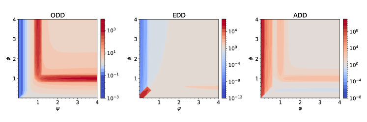
Phase Diagram. The phase diagram for the random projections model (Figure 1) offers richer insights into how model capacity, in interaction with the number of features and samples, affects bias amplification. In the $ODD$ and $EDD$ profiles, we observe apparent phase transitions at $\phi=\psi$ (when $\psi<0.5$) and $\psi=0.5$ (i.e., $\psi_{1}=\psi_{2}=1$), where these metrics begin decreasing significantly. In contrast, at $\psi=1$ and $\phi=1$, the $ODD$ seems to drastically increase. Furthermore, at $\phi=\psi$ (when $\psi<0.5$) and $\phi=0.5$ (when $\psi>0.5$), the $EDD$ greatly increases. Accordingly, in the $ADD$ profile, we observe apparent phase transitions at $\phi=\psi$ (when $\psi<0.5$), $\psi=0.5$, $\psi=1$, and $\phi=1$, where bias amplification begins occurring (i.e., $ADD>1$). However, bias seems to be consistently deamplified (i.e., $ADD<1$) at $\phi=\psi$ (when $\psi<0.5$) and $\phi=0.5$ (when $\psi>0.5$).

Figure 1: $ODD$, $EDD$, and $ADD$ phase diagrams for ridge regression with random projections. We plot the bias amplification phase diagrams with respect to $\phi$ (rate of features to samples) and $\psi$ (rate of parameters to samples), as predicted by our theory for ridge regression with random projections (Theorems 2, 3). Red regions indicate theoretical predictions greater than 1 (i.e., bias amplification in the rightmost plot), while blue regions indicate theoretical predictions less than 1 (i.e., bias deamplification in the rightmost plot). Darkness indicates intensity. We consider isotropic covariance matrices: $\Sigma_{1}=2I_{d},\Sigma_{2}=I_{d}$, $\Theta=2I_{d}$, $\Delta=I_{d}$. Additionally, $n=1\times 10^{4},\sigma_{1}^{2}=\sigma_{2}^{2}=1$. We further choose $\lambda=\lambda_{1}=\lambda_{2}=1\times 10^{-6}$ to approximate the minimum-norm interpolator. We show that bias amplification can occur even in the balanced data setting, i.e., when $p_{1}=p_{2}=1/2$.

4 Bias Amplification

We empirically show how ridge regression models with random projections may amplify bias when a single model is trained on a combination of data from different groups vs. when separate models are trained on data from each group (Bell & Sagun, 2023). We further show how our theory: (1) predicts bias amplification, and (2) exposes new, interesting bias amplification phenomena in various regimes.

4.1 Isotropic Covariance

Setup. To be consistent with the setting of Bell & Sagun (2023), we set different ground-truth weights for the groups ($\Theta=2I_{d},\Delta=I_{d}$). We additionally consider balanced data ($p_{1}=p_{2}=1/2$) without spurious correlations ($\Sigma_{1}=a_{1}I_{d},\Sigma_{2}=a_{2}I_{d}$, for $a_{1},a_{2}>0$). We further choose $\lambda=1\times 10^{-6}$ to approximate the minimum-norm interpolator; we henceforth set $\lambda=\lambda_{1}=\lambda_{2}$ for simplicity. We present other experimental details in Appendix I.1. We modulate $a_{1},a_{2},\sigma_{1}^{2},\sigma_{2}^{2}$, as well as $\psi$ (rate of parameters to samples) and $\phi$ (rate of features to samples) to understand the effects of model capacity and sample size on bias amplification. We consider diverse and dense values of these variables to obtain a clear picture of when and how models amplify bias.

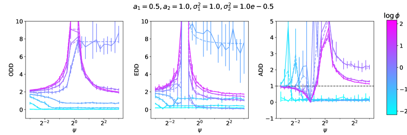
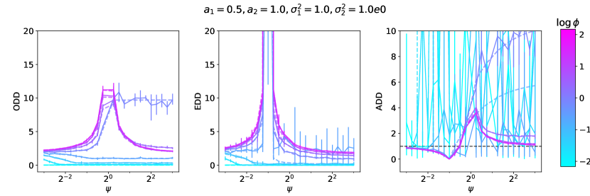
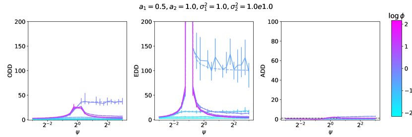
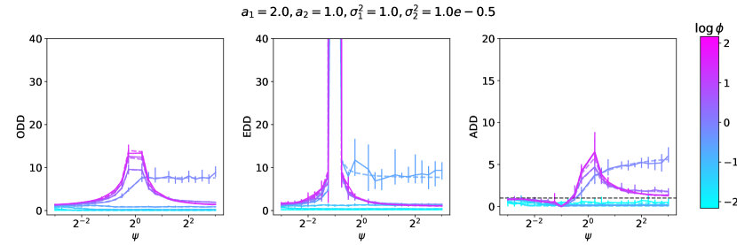
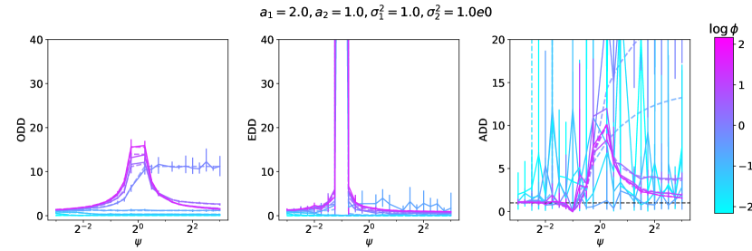
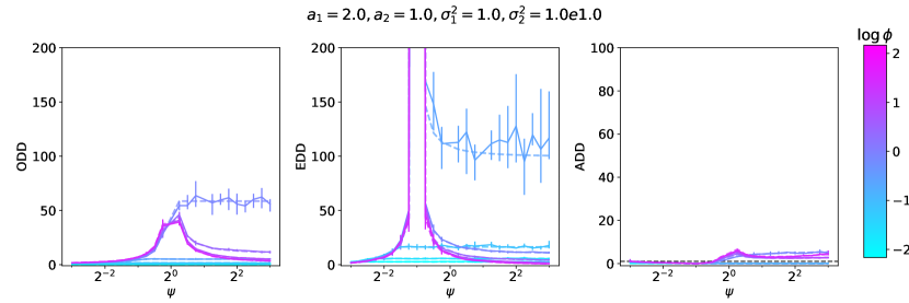
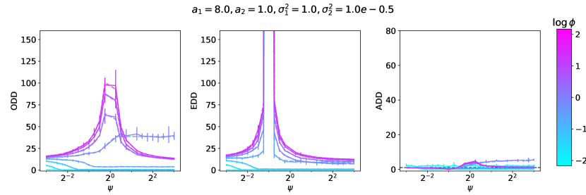
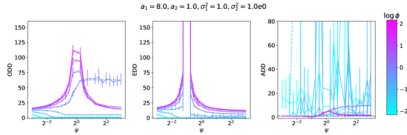
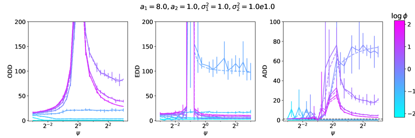
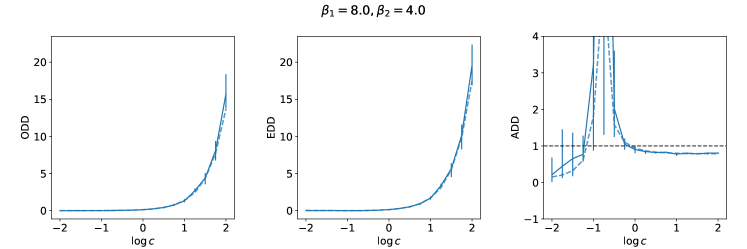
Validation of Theory. Figure 2 and the figures in Appendix J reveal that Theorems 2 and 3 closely predict the $ODD$, $EDD$, and $ADD$ of ridge regression models with random projections under diverse settings. As indicated by the error bars, some of our empirical estimates (especially those with larger magnitude) have higher variance and their variance is influenced by the choice of $\psi,\phi,a_{1},a_{2},\sigma_{1}^{2},\sigma_{2}^{2}$. Notably, our theory predicts the observation of Bell & Sagun (2023) that models can amplify bias even with balanced groups and without spurious correlations. We present new phenomena predicted by our theory below.

Effect of Label Noise. In the $ODD$ profile, the left tail is higher when the noise ratio $c=\sigma_{2}^{2}/\sigma_{1}^{2}$ is larger (compared to when it is lower), which suggests that under overparameterization, a larger noise ratio can increase disparities in test risk between groups when a single model is learned for both groups. We analytically explain this phenomenon in Appendix K. In contrast, the $EDD$ curve is generally higher for larger $c$, suggesting that a larger noise ratio increases disparities in test risk when a separate model is learned for each group. We replicate this finding on real data in Figure 3. Additionally, we observe that the $ADD$ grows faster close to the interpolation threshold for larger $c$, which suggests that a larger noise ratio can increase the maximum possible bias amplification.

Effect of Model Size. We observe interesting divergent behavior as $\psi$ (rate of parameters to samples) increases for different $\phi$ (rate of features to samples). When $\phi>1$, as $\psi$ increases, the $ODD$ increases and then decreases, peaking at the interpolation threshold at $\psi=1$. Similarly, when $\phi>0.5$ (i.e., $\phi_{1}=\phi_{2}>1$), as $\psi$ increases, the $EDD$ increases and then decreases, peaking at the interpolation threshold at $\psi=0.5$ (i.e., $\psi_{1}=\psi_{2}=1$). Accordingly, when $\phi>0.5$, bias is effectively deamplified (i.e., $ADD\ll 1$) at $\psi=0.5$ and when $\phi>1$, bias amplification peaks (i.e., $ADD\gg 1$) at $\psi=1$. In contrast, when $\phi<1$, the $ODD$ decreases as $\psi$ increases, plateauing at different finite values. Similarly, when $\phi<0.5$, the $EDD$ decreases and plateaus as $\psi$ increases. A notable exception to these trends occurs when $\phi\approx 1$, with the corresponding $ODD$ and $ADD$ curves consistently increasing as $\psi$ increases, plateauing at a significantly larger value (i.e., $ADD\gg 1$) than the curves corresponding to other values of $\psi$. Hence, overparameterization can greatly amplify bias when $\phi=1$. Regardless of the regime of $\phi$, the left tail of the $ADD$ profile appears to plateau at 1. The right tail plateaus at different finite values, with the curves corresponding to $\phi>1$ consistently plateauing above 1. This suggests that when $\phi>1$, overparameterization amplifies bias.

Effect of Number of Features. In the $ODD$ and $ADD$ profiles, when $\phi>1$, the right tail plateaus at higher values ($>1$) when $\phi$ is closer to 1. This suggests that with a similar number of features and samples, under overparameterization, bias amplification increases and may even be inevitable. In the $EDD$ profile, when $\phi>1$, the right tail plateaus at higher values when $\phi$ is larger. In contrast, when $\phi<1$, the right tail of the $ODD$ and $EDD$ curves plateaus at higher values when $\phi$ is larger. Regardless of the regime of $\phi$, the left tails of the $ODD$ and $EDD$ curves are higher for larger $\phi$.

Figure 2: Our theory predicts that models can amplify bias even with balanced groups and without spurious correlations. We empirically validate our theory (Theorems 2 and 3) for $ODD$, $EDD$, and $ADD$ under the setup described in Section 4.1, with $a_{1}=0.5,a_{2}=1,\sigma_{1}^{2}=1$, and $\sigma_{2}^{2}=1\times 10^{-5}$. The solid lines capture empirical values while the corresponding lower-opacity dashed lines represent what our theory predicts. We plot $ODD$ and $EDD$ on the same scale for easy comparison, and include a black dashed line at $ADD=1$ to contrast bias amplification vs. deamplification. We include the remaining plots with error bars in Appendix J.

4.2 Regularization and Training Dynamics

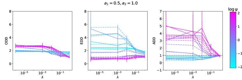
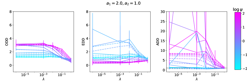
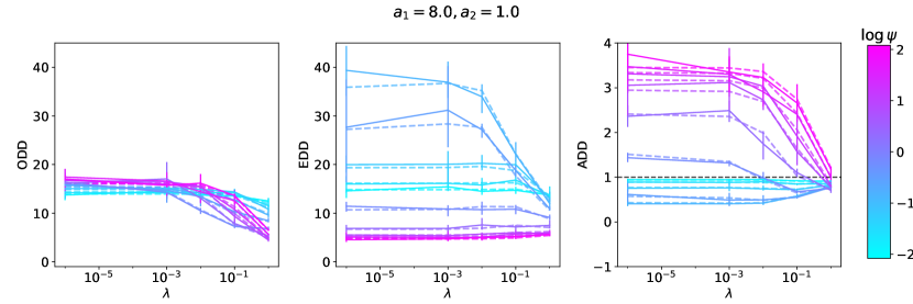
We now explore how regularization and training dynamics affect bias amplification.

Setup. We revisit the setting described in Section 4.1. We modulate $a_{1},a_{2},\psi$ (rate of parameters to samples), as well as $\lambda$ (regularization penalty) to understand the effects of regularization and early stopping on bias amplification. We fix $\sigma_{1}^{2}=\sigma_{2}^{2}=1$, and the rate of features to samples $\phi=0.75$.

Effect of Regularization and Training Time. We can simulate model learning over training time $t$ by setting $\lambda=1/t$ (Ali et al., 2019). In Figure 11 (in the appendix), we observe that regardless of the regime of $\psi$, $ADD\approx 1$ (i.e., there is neither bias amplification nor deamplification) when there is high regularization or a short training time. When $\psi>1$ (i.e., in the overparameterized regime), the $ADD$ is generally greater than 1 across values of $\lambda$ (i.e., bias is amplified), while when $\psi<1$ (i.e., in the underparameterized regime), the $ADD$ is less than 1 (i.e., bias is deamplified). Moreover, when $\psi>1$, as regularization decreases (or training time increases), bias amplification increases and plateaus. In contrast, when $\psi<1$, as regularization decreases (or training time increases), bias deamplification increases and plateaus. A notable exception to this trend occurs when $\psi$ is close to 1, where bias is initially deamplified and then amplified as $\lambda$ decreases (or $t$ increases). This suggests that there may be an optimal regularization penalty or training time to avoid bias amplification and increase bias deamplification. This aligns with the findings of Hall et al. (2022) and Jain et al. (2024) that bias amplification can vary substantially during training; future work can establish stronger connections between our theoretical results and the results of Jain et al., who identify phases in the evolution of bias and a crossing phenomenon in the test error curves of groups during training. Intuitively, as training progresses, overparameterized models may discover “shortcut” associations that do not generalize equally well across groups, yielding bias amplification (Geirhos et al., 2020).

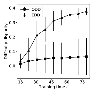
Corroboration on Real Data. We further investigate the effect of training time on bias amplification on a more realistic dataset. We train a convolutional neural network (CNN) on Colored MNIST (see Appendix I.2 for more details). Colored MNIST is a semi-synthetic dataset derived from MNIST where digits are randomly re-colored to be red or green (Arjovsky et al., 2019). We treat the color of each digit as its group, and we manipulate the groups to have different levels of label noise. In our experimental protocol: (1) the color of each digit (in both train and test) is chosen uniformly at random (i.e., with probability 0.5) and independently of the label; (2) the labels of red digits are flipped with probability 0.05 while the labels of green digits are flipped with probability 0.25; (3) labels are binarized (i.e., digits 0-4 correspond to 0 while digits 5-9 correspond to 1); and (4) each training step constitutes a step of gradient descent based on a batch of 250 instances. Although Colored MNIST is a classification task and we use a complex CNN architecture, our theory correctly predicts that as the training time $t$ increases, the $ODD$ of the CNN is relatively low while the $EDD$ is much larger, producing bias deamplification (Figure 3).

Figure 3: Our theory predicts that disparate label noise between groups deamplifies bias on Colored MNIST. We plot the $ODD$ and $EDD$ of a CNN over training time $t$ for Colored MNIST. As $t$ increases, the $ODD$ is relatively low while the $EDD$ is noticeably higher. Please refer to Figure 6 (in the appendix) for error bars.

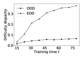
Taking $t\to\infty$ corresponds to the setting of $\lambda\to 0^{+}$ in our theory (Theorems 2, 3). Because we assign the colors at random, the only difference in image features between groups would be color; therefore, we expect the covariance matrices $\Sigma_{1}$ and $\Sigma_{2}$ to coincide and $\Delta=0$ (i.e., $w_{1}^{*}=w_{2}^{*}$). Note that we do not make any assumptions about the structure of $\Sigma_{1},\Sigma_{2}$. Furthermore, $p_{1}=p_{2}=1/2$, and thus, $\phi_{1}=\phi_{2}$ and $\psi_{1}=\psi_{2}$. Additionally, we analogize the probability of label flipping to label noise in ridge regression. Hence, $e_{1}=e_{2},u_{1}=u_{2}$. Accordingly, $\lim_{\lambda\to 0^{+}}B_{1}(\widehat{f})=\lim_{\lambda\to 0^{+}}B_{1}(\widehat{f}_{1})\approx\lim_{\lambda\to 0^{+}}B_{2}(\widehat{f})=\lim_{\lambda\to 0^{+}}B_{2}(\widehat{f}_{2})$. Simultaneously, $\lim_{\lambda\to 0^{+}}V_{1}(\widehat{f})\approx\lim_{\lambda\to 0^{+}}V_{2}(\widehat{f})$. However, $\lim_{\lambda\to 0^{+}}V_{1}(\widehat{f}_{1})\approx\sigma_{1}^{2}/2\cdot V=0.05/2\cdot V=0.025V$ (where $V=\phi_{1}h_{1}^{(2)}(I_{d},\Sigma)$), while $\lim_{\lambda\to 0^{+}}V_{2}(\widehat{f}_{2})\approx\sigma_{2}^{2}/2\cdot V=0.25/2\cdot V=0.125V$. This results in $ODD\approx 0$ while $EDD\approx 0.1|V|$, which explains the divergence of $ODD$ and $EDD$ in Figure 3. Intuitively, the high label noise for group 2 prohibits the separate model $\widehat{f}_{2}$ from achieving a low test risk compared to $\widehat{f}_{1}$; the single model $\widehat{f}$ achieves a comparable test risk on both groups, effectively deamplifying bias, because of learning signals from both groups.

5 Minority-Group Error

Recent work has revealed that overparameterization may hurt test performance on minority groups due to spurious features (Sagawa et al., 2020; Khani & Liang, 2021). Our theory provides new insights into how model size and extraneous features affect minority-group error.

Setup. To be consistent with the settings of (Sagawa et al., 2020; Khani & Liang, 2021), we consider diatomic covariance matrices consisting of core and extraneous features. In particular, we define $A\oplus B=\begin{pmatrix}A&0\\ 0&B\end{pmatrix}$, and choose $\Sigma_{1}=a_{1}I_{\pi d}\oplus 0I_{(1-\pi)d},\Sigma_{2}=a_{2}I_{\pi d}\oplus b_{2}I_{(1-\pi)d}$, for $\pi\in(0,1)$ and $a_{1},b_{2}>0$ and $a_{1}=a_{2}$. Here, the first $\pi d$ features represent common core features of groups 1 and 2 while the latter $(1-\pi)d$ features capture unshared extraneous features for group 2 (e.g., spurious features). Intuitively, this setting can model: (1) learning from data from two groups where one group suffers from spurious features (Sagawa et al., 2020), or (2) learning from a mixture of raw data (i.e., with spurious features) and clean data (i.e., without spurious features) for a single population (Khani & Liang, 2021). We ask: Does our theory predict how the inclusion of different amounts of extraneous features affect the test risk of the minority group when a single model is trained on data from both groups vs. a separate model is trained per group?

Although Sagawa et al. (2020) consider classification instead of regression, to closely mirror their experimental setting, we pick $p_{1}=0.9$ (i.e., group 1 is much larger than group 2) and $\Theta=I_{d},\Delta=0$ (i.e., $w_{1}^{*}=w_{2}^{*}$). We additionally choose $\lambda=1\times 10^{-6}$ and $\sigma_{1}^{2}=\sigma_{2}^{2}=1$. We modulate $a_{1},b_{2}$, as well as $\psi$ (rate of parameters to samples) and $\phi$ (rate of features to samples). Notably, this setting also captures learning problems with $o(d)$ overlapping core and extraneous features in our asymptotic scaling limit. An extremization of this setting is choosing $\Sigma_{1}=a_{1}I_{\pi d}\oplus 0I_{(1-\pi)d},\Sigma_{2}=0I_{\pi d}\oplus b_{2}I_{(1-\pi)d}$, where groups 1 and 2 have entirely different sets of important features.

Figure 4: Minority-group test risk can peak with different model sizes depending on the rate of features to samples. We empirically demonstrate that minority-group bias is affected by extraneous features. We validate our theory (Theorems 2 and 3) for together $R_{1},R_{2}$ (i.e., single model learned for both groups) and separate $R_{1},R_{2}$ (i.e., separate model learned per group) under the setup described in Section 4.2, with $a_{1}=2,b_{2}=0.2$, and $\pi=0.5$. The solid lines capture empirical values while the corresponding lower-opacity dashed lines represent what our theory predicts. We include a black dashed line at $ADD=1$ to contrast bias amplification vs. deamplification. All y-axes are on the same scale for easy comparison. The remaining plots with error bars are in Appendix N.

Interpolation Thresholds. The together test risk $R_{2}$ for the minority group has different interpolation thresholds as $\psi$ increases depending on $\phi$ and $\pi$ (fraction of core features). Notably, as $\phi$ increases, the interpolation thresholds occur at larger model sizes, culminating at $\psi=1$. This suggests that for a higher rate of features to samples, a larger model size can greatly increase the together test risk of group 2. Furthermore, the interpolation thresholds all occur closer to $\psi=1$ for larger $\pi$, collapsing to a single threshold at $\psi=1$ when $\pi\to 1$ as in Appendix J. Therefore, a lower fraction of core features can yield more possible model sizes that increase the test risk of group 2. In addition, the together $R_{2}$ exhibits a steeper rate of growth around the interpolation thresholds for larger $b_{2}$, suggesting that a higher variance in the extraneous features can also increase the together test risk of group 2. The phenomenon of different interpolation thresholds is not visible for $R_{2}$ when a separate model is trained per group, nor for $R_{1}$.

Overparameterization. The right tails of the together $R_{2}$ curves plateau at different horizontal values depending on $\phi$. In particular, for $\phi$ closer to 1, the $R_{2}$ curves plateau at a higher value, suggesting that a similar number of features and samples can exacerbate minority-group error under overparameterization. Furthermore, when $\phi$ is close to 1, the together $R_{1}$ curves plateau at lower values than their corresponding together $R_{2}$ curves; this suggests that there can be fundamental differences in test error between groups, and thus fundamental model biases, that do not disappear even with increased model capacity. This phenomenon diminishes as the fraction of core features increases, and is not visible in the separate $R_{2}$ curves. Our experiments support the finding of Sagawa et al. (2020) that overparameterization with spurious features increases test risk disparities between groups, and we nuance this finding by identifying that this phenomenon is most prominent in the regime where the number of features tends towards the number of samples.

6 Conclusion

In this paper, we present a unifying, rigorous, and effective theory of machine learning bias in the settings of ridge regression with and without random projections. We extensively empirically validate our theory in diverse settings. We further demonstrate that our theory provides interesting insights into bias amplification and minority-group error in various regimes. For example, there may be an optimal regularization penalty or training time to avoid bias amplification, and there can be fundamental differences in test error between groups that do not vanish with increased parameterization. These findings can inform strategies to evaluate and mitigate unfairness in machine learning.

Our methods and theory are easily extendable to analyze the case of more than two groups and can accommodate label noise sampled from various distributions. However, our theory is not directly extendable to different proportionate scaling limits, e.g., $d^{2}/n$ has a finite limit instead of $d/n$. Additionally, our theory requires approximately normally-distributed data and thus does not currently account for missing features, which are common in the real world (Feng et al., 2024). Furthermore, our theory implicitly assumes that group information is known, which is not always true (Coston et al., 2019); however, because we work in an asymptotic scaling limit, having access to group information with $o(\min(n_{1}),\min(n_{2}))$ noise is sufficient. As future work, we can leverage “Gaussian equivalents” (Goldt et al., 2022) to extend our theory to wide, fully-trained networks in the NTK (Jacot et al., 2018) and lazy (Chizat et al., 2019) regimes; this will enable us to understand how, apart from model size, other design choices like activation functions and learning rate may affect bias amplification.

Appendix

Appendix A Warm-up: Deriving Marchenko-Pastur Law via
Operator-Valued Free Probability Theory

We provide a detailed example of how to apply linear pencils and operator-valued free probability theory to derive the Marchenko-Pastur law. Let $S=(1/n)X^{\top}X\in\mathbb{R}^{d\times d}$, the empirical covariance matrix for an $n\times d$ random matrix $X$ with IID entries from ${\cal N}(0,1)$. If $n$ tends to infinity while $d$ is held fixed, then $S$ converges to the population covariance matrix, here $\Sigma=I_{d}$. If $d$ also tends to infinity, then the limit seizes to exist. It turns out that one can still make sense of the limiting distribution of eigenvalues of $S$ in case $d/n$ stays constant, namely the behavior of the random histogram:

$$\widehat{\mu}_{n}=\frac{1}{d}\sum_{i=1}^{n}\delta_{\widehat{\lambda}_{i}},$$ (32)

where $\widehat{\lambda}_{1},\ldots,\widehat{\lambda}_{d}$ are the eigenvalues of $S$. Let us state without any delay that in the aforementioned limit, i.e.,

$$n,d\to\infty,\,d/n\to\gamma\in(0,\infty),$$ (33)

$\widehat{\mu}_{n}$ converges to a deterministic law $\mu_{\text{MP}}$ on $\mathbb{R}$ called the Marchenko-Pastur law. This is central to the field of random matrix theory (RMT), a central tool in probability theory, statistical analysis of neural networks, finance, etc. We are interested in an even more powerful tool – free probability theory (FPT) – is powerful enough to give a precise picture of deep learning in certain linearized regimes (e.g., random features, NTK, etc.) and interesting phenomena (e.g., triple descent, etc.) via analytic calculation.

A.1 Step 1: Constructing a Linear Pencil

For any positive $\lambda$, consider the $2\times 2$ block matrix $Q$ defined by:

$$Q=\begin{pmatrix}I_{n}&-\frac{X}{\sqrt{n\lambda}}\\ \frac{X^{\top}}{\sqrt{n\lambda}}&I_{d}\end{pmatrix}.$$ (34)

Let $\bar{\operatorname{tr}}\,$ be the normalized trace operator on square matrices and set $\varphi=\mathbb{E}\circ\bar{\operatorname{tr}}\,$. This gives random $(n+d)\times(n+d)$ matrices the structure of a von Neumann algebra $\mathcal{A}$. Define a $2\times 2$ matrix $G=G(Q)$ by:

$$G=\mathbb{(}I_{2}\otimes\varphi)Q^{-1},\text{ i.e }g_{i,j}=\varphi([Q^{-1}]_{i,j})=[\varphi(Q^{-1})]_{i,j}\text{ for all }i,j\in\{1,2\}.$$ (35)

Thus, the operator $(I_{2}\otimes\varphi)Q^{-1}$ extracts the expectation of the normalized trace of the blocks of the inverse of the a $2\times 2$ block matrix $Q$.

Observe that:

$$\mathbb{E}\,\bar{\operatorname{tr}}\,(S+\lambda I_{d})^{-1}=\frac{g_{2,2}}{\lambda}.$$ (36)

This is a direct consequence of inverting a $2\times 2$ block matrix (Schur’s complement). The mechanical advantage of equation 36 is that the resolvent $(S+\lambda I_{d})^{-1}$ depends quadratically on $X$ while $g_{2,2}$ is defined via $Q$, which is linear in $X$. For this reason, $Q$ is called a linear pencil for $(S+\lambda I_{d})^{-1}$. The construction of appropriate linear pencils rational functions of random matrices is a crucial step in leveraging FPT.

A.2 Step 2: Constructing the Fundamental Equation via Freeness

For any $B\in M_{b}(\mathbb{C})^{+}$ (here $b\times b$ is the number of blocks in the linear pencil $Q_{X}$, and so $b=2$), define a block matrix $B\otimes 1_{\mathcal{A}}$ by:

$$[B\otimes 1_{\mathcal{A}}]_{ij}=\begin{cases}b_{ij}I_{d_{i}},&\mbox{ if }d_{i}=d_{j},\\ 0,&\mbox{ else.}\end{cases}$$ (37)

Now, observe that we can write $Q=F-Q_{X}$, where:

$$F=\begin{pmatrix}I_{d}&0\\ 0&I_{n}\end{pmatrix}=I_{2}\otimes 1_{\mathcal{A}}\text{ and }Q_{X}=\begin{pmatrix}0&\frac{X}{\sqrt{n\lambda}}\\ -\frac{X^{\top}}{\sqrt{n\lambda}}&0\end{pmatrix}.$$ (38)

One can then express $G=(I_{b}\otimes\varphi)Q^{-1}=(I_{b}\otimes\varphi)(F-Q_{X})^{-1}$. From operator-valued FPT, we know that in the proportionate scaling limit equation 33, the following fixed-point equation (due to the asymptotic freeness of $Q_{X}$ and $F$) is satisfied by $G$:

$$G=(I_{b}\otimes\varphi)(F-R\otimes 1_{\mathcal{A}})^{-1},$$ (39)

where $R=\mathcal{R}_{Q_{X}}(G)$, and $R_{Q_{X}}$ is the R-transform of $Q_{X}$ which maps $M_{b}(\mathbb{C})^{+}$ to itself like so:

$$\mathcal{R}_{Q_{X}}(B)_{ij}=\sum_{k,\ell}\sigma(i,k;\ell,j)\alpha_{k}b_{k\ell}.$$ (40)

Here, $\sigma(i,k;\ell,j)$ is the covariance between the entries of block $(i,k)$ and block $(\ell,j)$ of $Q_{X}$, while $\alpha_{k}$ is the dimension of the block $(k,\ell)$.

A.3 Step 3: The Final Calculation

Due to the structure of $Q_{X}$, one computes from equation 40:

$$r_{1,1} =d\cdot\frac{-1}{n\lambda}g_{2,2}=-\frac{\gamma}{\lambda}g_{2,2},$$ (41)

$$r_{1,2} =0,$$ (42)

$$r_{2,1} =0,$$ (43)

$$r_{2,2} =n\cdot\frac{-1}{n\lambda}g_{1,1}=-\frac{1}{\lambda}g_{1,1}.$$ (44)

Combining this with equation 39, one has:

$$\begin{split}G=(I_{2}\otimes\varphi)(Z-R\otimes 1_{\mathcal{A}})^{-1}=(I_{2}-R)^{-1}&=\begin{pmatrix}1+(\gamma/\lambda)g_{2,2}&0\\ 0&1+g_{2,2}/\lambda\end{pmatrix}^{-1}\\ &=\begin{pmatrix}\lambda/(\lambda+\gamma g_{2,2})&0\\ 0&\lambda/(\lambda+g_{1,1})\end{pmatrix}.\end{split}$$ (45)

Comparing the matrix entries, this translates to the following scalar equations:

$$g_{1,1} =\frac{\lambda}{\lambda+\gamma g_{2,2}},$$ (46)

$$g_{2,2} =\frac{\lambda}{\lambda+g_{1,1}},$$ (47)

$$\ g_{2,1} =g_{1,2}=0.$$ (48)

Plugging the second equation into the first (to eliminate $g_{1,1}$) gives:

$$g_{2,2}=\dfrac{\lambda}{\lambda+\lambda/(\lambda+\gamma g_{2,2})}.$$

Setting $m=g_{2,2}/\lambda$ then gives $m=(\lambda+1/(1+\gamma m))^{-1}$, i.e.:

$$\frac{1}{m}=\lambda+\frac{1}{1+\gamma m},$$ (49)

which is precisely the functional equation characterizing the Stieltjes transform (evaluated at $\lambda=-z$) of the Marchenko-Pastur law with shape parameter $\gamma$. By treating $\lambda$ as a complex number and applying the Cauchy-inversion formula, we can recover $\mu_{\text{MP}}$.

Appendix B Technical Assumptions

Assumption 3.

The per-group covariance matrices $\Sigma_{1}$ and $\Sigma_{2}$ and ground-truth weight covariance matrices $\Theta$ and $\Delta$ are all simultaneously diagonalizable; hence, all these matrices commute.

While Assumption 3 may appear reductive, our goal is to analyze the bias amplification phenomenon in a sufficient setting that does not introduce complexities due to non-commutativity.

Assumption 4.

We assume the following spectral densities exist when $d\to\infty$:

• $\nu\in\mathcal{P}(\mathbb{R}_{+})$ is the limiting spectral density of $\Sigma_{2}\Sigma_{1}^{-1}$, of the ratios $\lambda_{j}^{(2)}/\lambda_{j}^{(1)}$ of the eigenvalues of the respective covariance matrices,

• $\mu\in\mathcal{P}(\mathbb{R}_{+})$ is the joint limiting density of the spectra of $\Sigma_{2}\Sigma_{1}^{-1}$ and $\Sigma_{1}$

• $\pi\in\mathcal{P}(\mathbb{R}_{+})$ is the limiting density of the spectrum of $\Delta$.

Appendix C Theorem 4: Separate Classical Model Learned Per Group

Suppose that the classical ridge regression models $\widehat{f}_{1}$ and $\widehat{f}_{2}$ are learned using empirical risk minimization and $\ell_{2}$-regularization with penalties $\lambda_{1}$ and $\lambda_{2}$, respectively. In particular, we have the following optimization problem for each group $s$:

$$\arg\min_{w\in\mathbb{R}^{d}}L(w)=\frac{1}{n_{s}}\sum_{(x_{i},y_{i})\in\mathcal{D}^{s}}(x_{i}^{\top}w-y_{i})^{2}+\lambda_{s}\|w\|^{2}=\frac{\|X_{s}w-Y_{s}\|^{2}_{2}}{n_{s}}+\lambda_{s}\|w\|^{2}.$$ (50)

We first present some relevant definitions.

Definition 4.

Let $\bar{\operatorname{df}}_{m}^{(s)}(t)=\bar{\operatorname{tr}}\,\Sigma_{s}^{m}\left(\Sigma_{s}+tI_{d}\right)^{-m}$, and $\kappa_{s}$ be the unique positive solution to the equation $\kappa_{s}-\lambda_{s}=\kappa_{s}\phi_{s}\bar{\operatorname{df}}^{(s)}_{1}(\kappa_{s}).$

In this setting, we deduce Theorem 4. We derive Theorems 4 and 1 using OVFPT, which is sufficiently powerful to give the general case in which we are interested (i.e., two groups with general $p_{s},\Sigma_{s}$). Theorems 4 and1 are non-trivial generalizations of Proposition 3 from (Bach, 2024), which can be recovered by taking $p_{s}\to 1$ (i.e., $p_{s^{\prime}}\to 0$).

Theorem 4.

Under Assumptions 3 and 1, it holds that:

$$R_{s}(\widehat{f}_{s})\simeq B_{s}(\widehat{f}_{s})+V_{s}(\widehat{f}_{s}),\text{ with }$$ (51)

$$V_{s}(\widehat{f}_{s})=\frac{\sigma_{s}^{2}\phi_{s}\bar{\operatorname{df}}_{2}^{(s)}(\kappa_{s})}{1-\phi_{s}\bar{\operatorname{df}}_{2}^{(s)}(\kappa_{s})},\,B_{s}(\widehat{f}_{s}) =\frac{\kappa_{s}^{2}\bar{\operatorname{tr}}\,\Theta_{s}\Sigma_{s}\left(\Sigma_{s}+\kappa_{s}I_{d}\right)^{-2}}{1-\phi_{s}\bar{\operatorname{df}}_{2}^{(s)}(\kappa_{s})},\,\Theta_{1}=\Theta,\,\Theta_{2}=\Theta+\Delta.$$ (52)

Proof.

We define $M_{s}=X_{s}^{\top}X_{s}$. Note that $\widehat{w}_{s}=X_{s}^{\dagger}Y_{s}=(X_{s}^{\top}X_{s}+n_{s}\lambda_{s}I_{d})^{-1}X_{s}^{\top}(X_{s}w^{*}_{s}+E_{s})=(M_{s}+n_{s}\lambda_{s}I_{d})^{-1}M_{s}w^{*}_{s}+(M_{s}+n_{s}\lambda_{s}I_{d})^{-1}X_{s}^{\top}E_{s}$. We deduce that $R_{s}(\widehat{f}_{s})=B_{s}(\widehat{f}_{s})+V_{s}(\widehat{f}_{s})$, where:

$$B_{s}(\widehat{f}_{s}) =\mathbb{E}\,\|(M_{s}+n_{s}\lambda_{s}I_{d})^{-1}M_{s}w^{*}_{s}-w^{*}_{s}\|_{\Sigma_{s}}^{2},$$ (53)

$$V_{s}(\widehat{f}_{s}) =\mathbb{E}\,\|(M_{s}+n_{s}\lambda_{s}I_{d})^{-1}X_{s}^{\top}E_{s}\|_{\Sigma_{s}}^{2}.$$ (54)

C.1 Variance Term

Note that the variance term $V_{s}(\widehat{f})$ of the test error of $\widehat{f}_{s}$ evaluated on group $s$ is given by:

$$V_{s}(\widehat{f}_{s}) =\sigma_{s}^{2}\mathbb{E}\,\operatorname{tr}\,X_{s}(M_{s}+n_{s}\lambda_{s}I_{d})^{-1}\Sigma_{s}(M_{s}+n_{s}\lambda_{s}I_{d})^{-1}X_{s}^{\top}$$ (55)

$$=\sigma_{s}^{2}\mathbb{E}\,\operatorname{tr}\,(M_{s}+n_{s}\lambda_{s}I_{d})^{-1}M_{s}(M_{s}+n_{s}\lambda_{s}I_{d})^{-1}\Sigma_{s}.$$ (56)

We can re-express this as:

$$n_{s}V_{s}(\widehat{f}_{s}) =\sigma_{s}^{2}\mathbb{E}\operatorname{tr}\,(H_{s}+\lambda_{s}I_{d})^{-1}H_{s}(H_{s}+\lambda_{s}I_{d})^{-1}\Sigma_{s}$$ (57)

$$=\frac{\sigma_{s}^{2}}{\lambda_{s}}\mathbb{E}\operatorname{tr}\,(H_{s}/\lambda_{s}+I_{d})^{-1}(H_{s}/\lambda_{s})(H_{s}/\lambda_{s}+I_{d})^{-1}\Sigma_{s},$$ (58)

where $H_{s}=X_{s}^{\top}X_{s}/n_{s}$ and $X_{s}=Z_{s}\Sigma_{s}^{1/2}$, with $Z_{1}\in\mathbb{R}^{n_{1}\times d}$ and $Z_{2}\in\mathbb{R}^{n_{2}\times d}$ being independent random matrices with IID entries from ${\cal N}(0,1)$. The typical variance term is proportional to:

$$\bar{\operatorname{tr}}\,(H_{s}+\lambda_{s}I_{d})^{-1}H_{s}(H_{s}+\lambda_{s}I_{d})^{-1}\Sigma_{s}.$$ (59)

WLOG, we consider the case where $s=1$. The matrix of interest has a linear pencil representation given by (with zero-based indexing):

$$(H_{1}/\lambda_{1}+I_{d})^{-1}(H_{1}/\lambda_{1})(H_{1}/\lambda_{1}+I_{d})^{-1}\Sigma_{1}=Q^{-1}_{0,8},$$ (60)

where the linear pencil $Q$ is defined as follows:

$$Q=\leavevmode\resizebox{346.89731pt}{}{$\left(\begin{array}[]{ccccccccc}I_{d}&\Sigma_{1}^{\frac{1}{2}}&0&0&-\Sigma_{1}^{\frac{1}{2}}&0&0&0&0\\ 0&I_{d}&-\frac{1}{\sqrt{\lambda_{1}}\sqrt{n_{1}}}Z_{1}^{\top}&0&0&0&0&0&0\\ 0&0&I_{n_{1}}&-\frac{1}{\sqrt{\lambda_{1}}\sqrt{n_{1}}}Z_{1}&0&0&0&0&0\\ -\Sigma_{1}^{\frac{1}{2}}&0&0&I_{d}&0&0&0&0&0\\ 0&0&0&0&I_{d}&-\frac{1}{\sqrt{\lambda_{1}}\sqrt{n_{1}}}Z_{1}^{\top}&0&0&0\\ 0&0&0&0&0&I_{n_{1}}&-\frac{1}{\sqrt{\lambda_{1}}\sqrt{n_{1}}}Z_{1}&0&0\\ 0&0&0&0&0&0&I_{d}&-\Sigma_{1}^{\frac{1}{2}}&0\\ 0&0&0&0&\Sigma_{1}^{\frac{1}{2}}&0&0&I_{d}&-\Sigma_{1}\\ 0&0&0&0&0&0&0&0&I_{d}\\ \end{array}\right)$}.$$ (70)

We compute $Q$ using the NCMinimalDescriptorRealization function of the NCAlgebra library. We further symmetrize $Q$ by constructing the self-adjoint matrix $\overline{Q}$:

$$\overline{Q}=\left(\begin{array}[]{cc}0&Q^{\top}\\ Q&0\end{array}\right).$$ (73)

This enables us to apply known formulas for the $R$-transform of Gaussian block matrices (Far et al., 2006). We note that $\overline{Q}^{-1}_{0,17}=Q^{-1}_{0,8}$. Taking similar steps as Lee et al. (2023), we use operator-valued free probability theory (OVFPT) on $\overline{Q}$. Let $G=(I_{18}\otimes\mathbb{E}\,\bar{\operatorname{tr}}\,)\overline{Q}^{-1}\in\mathbb{R}^{18\times 18}$ be the matrix whose entries are normalized traces of blocks of $\overline{Q}^{-1}$. We provide a detailed example of how to apply linear pencils and operator-valued free probability theory to derive the Marchenko-Pastur law in Appendix A. One can arrive at that, in the asymptotic limit given by equation 9, the following holds:

$$\begin{split}&\mathbb{E}\bar{\operatorname{tr}}\,(H_{1}+\lambda_{1}I_{d})^{-1}H_{1}(H_{1}+\lambda_{1}I_{d})^{-1}\Sigma_{1}=\frac{G_{0,17}}{\lambda_{1}},\\ &\text{ with }\frac{G_{0,17}}{\lambda_{1}}=(G_{5,14}-G_{2,14})\bar{\operatorname{tr}}\,\left(\Sigma_{1}G_{2,11}+\lambda_{1}I_{d}\right)^{-1}\Sigma_{1}\left(\Sigma_{1}G_{5,14}+\lambda_{1}I_{d}\right)^{-1}\Sigma_{1}.\end{split}$$ (74)

We will now obtain the fixed-point equations satisfied by $G_{2,11}$ and $G_{5,14}$. We observe that:

$$G_{2,11}=-\frac{\lambda_{1}}{-\lambda_{1}+\phi_{1}G_{3,10}},\quad G_{3,10}=-\lambda_{1}\bar{\operatorname{tr}}\,\Sigma_{1}(\Sigma_{1}G_{2,11}+\lambda_{1}I_{d})^{-1}$$ (75)

$$\implies G_{2,11}=\frac{1}{1+\phi_{1}\bar{\operatorname{tr}}\,\Sigma_{1}(\Sigma_{1}G_{2,11}+\lambda_{1}I_{d})^{-1}},$$ (76)

$$G_{5,14}=-\frac{\lambda_{1}}{-\lambda_{1}+\phi_{1}G_{6,13}},\quad G_{6,13}=-\lambda_{1}\bar{\operatorname{tr}}\,\Sigma_{1}\left(\Sigma_{1}G_{5,14}+\lambda_{1}I_{d}\right)^{-1}$$ (77)

$$\implies G_{5,14}=\frac{1}{1+\phi_{1}\bar{\operatorname{tr}}\,\Sigma_{1}\left(\Sigma_{1}G_{5,14}+\lambda_{1}I_{d}\right)^{-1}}.$$ (78)

We recognize that we must have the identification $e_{1}=G_{2,11}=G_{5,14}$, where $e_{1}\geq 0$. Therefore:

$$e_{1} =\frac{e_{1}}{e_{1}+\phi_{1}\bar{\operatorname{df}}^{(1)}_{1}(\lambda_{1}/e_{1})}$$ (79)

$$\text{i.e., }1 =e_{1}+\phi_{1}\bar{\operatorname{df}}^{(1)}_{1}(\lambda_{1}/e_{1})=\lambda_{1}/\kappa_{1}+\phi_{1}\bar{\operatorname{df}}^{(1)}_{1}(\kappa_{1})$$ (80)

$$\kappa_{1} =\lambda_{1}+\kappa_{1}\phi_{1}\bar{\operatorname{df}}^{(1)}_{1}(\kappa_{1}),$$ (81)

where $\bar{\operatorname{df}}_{m}^{(s)}(t)=\bar{\operatorname{tr}}\,\Sigma_{s}^{m}\left(\Sigma_{s}+tI_{d}\right)^{-m}$ and $\kappa_{1}=\lambda_{1}/e_{1}$. Additionally:

$$G_{2,14} =\frac{\lambda_{1}\phi_{1}G_{3,13}}{(-\lambda_{1}+\phi_{1}G_{3,10})(-\lambda_{1}+\phi_{1}G_{6,13})}=\phi_{1}e_{1}^{2}\frac{G_{3,13}}{\lambda_{1}},$$ (82)

$$\frac{G_{3,13}}{\lambda_{1}} =\bar{\operatorname{tr}}\,(\Sigma_{1}G_{2,11}+\lambda_{1}I_{d})^{-2}(\Sigma_{1}G_{2,14}+\lambda_{1}I_{d})\Sigma_{1}$$ (83)

$$=\frac{G_{2,14}}{e_{1}^{2}}\bar{\operatorname{df}}_{2}^{(1)}(\kappa_{1})+\lambda_{1}\bar{\operatorname{tr}}\,(\Sigma_{1}e_{1}+\lambda_{1}I_{d})^{-2}\Sigma_{1},$$ (84)

$$\frac{G_{3,10}}{\lambda_{1}} =-\bar{\operatorname{tr}}\,(\Sigma_{1}e_{1}+\lambda_{1}I_{d})^{-1}\Sigma_{1}.$$ (85)

Then:

$$G_{5,14}-G_{2,14} =e_{1}^{2}\left(1-\phi_{1}\frac{G_{3,10}+G_{3,13}}{\lambda_{1}}\right),$$ (86)

$$\frac{G_{3,10}+G_{3,13}}{\lambda_{1}} =\frac{G_{2,14}}{e_{1}^{2}}\bar{\operatorname{df}}_{2}^{(1)}(\kappa_{1})+\lambda_{1}\bar{\operatorname{tr}}\,(\Sigma_{1}e_{1}+\lambda_{1}I_{d})^{-2}\Sigma_{1}$$ (87)

$$-\bar{\operatorname{tr}}\,(\Sigma_{1}e_{1}+\lambda_{1}I_{d})^{-2}(\Sigma_{1}e_{1}+\lambda_{1}I_{d})\Sigma_{1}$$ (88)

$$=\frac{G_{2,14}}{e_{1}^{2}}\bar{\operatorname{df}}_{2}^{(1)}(\kappa_{1})-\frac{e_{1}}{e_{1}^{2}}\bar{\operatorname{df}}_{2}^{(1)}(\kappa_{1})$$ (89)

$$=-\frac{G_{5,14}-G_{2,14}}{e_{1}^{2}}\bar{\operatorname{df}}_{2}^{(1)}(\kappa_{1}).$$ (90)

We define:

$$c_{1}\geq 1,c_{1}=\frac{G_{5,14}-G_{2,14}}{e_{1}^{2}}=1+\phi_{1}c_{1}\bar{\operatorname{df}}_{2}^{(1)}(\kappa_{1}),$$ (91)

i.e., $$c_{1}=\frac{1}{1-\phi_{1}\bar{\operatorname{df}}_{2}^{(1)}(\kappa_{1})}.$$ (92)

Hence:

$$\frac{G_{0,17}}{\lambda_{1}}=c_{1}\bar{\operatorname{df}}_{2}^{(1)}(\kappa_{1})=\frac{\bar{\operatorname{df}}_{2}^{(1)}(\kappa_{1})}{1-\phi_{1}\bar{\operatorname{df}}_{2}^{(1)}(\kappa_{1})}.$$ (93)

In conclusion:

$$\kappa_{1}=\lambda_{1}+\kappa_{1}\phi_{1}\bar{\operatorname{df}}^{(1)}_{1}(\kappa_{1}),$$ (94)

$$V_{1}(\widehat{f}_{1})=\frac{\sigma_{1}^{2}\phi_{1}\bar{\operatorname{df}}_{2}^{(1)}(\kappa_{1})}{1-\phi_{1}\bar{\operatorname{df}}_{2}^{(1)}(\kappa_{1})}.$$ (95)

Following similar steps for $V_{2}(\widehat{f}_{2})$, we get:

$$\kappa_{2}=\lambda_{2}+\kappa_{2}\phi_{2}\bar{\operatorname{df}}^{(2)}_{1}(\kappa_{2}),$$ (96)

$$V_{2}(\widehat{f}_{2})=\frac{\sigma_{2}^{2}\phi_{2}\bar{\operatorname{df}}_{2}^{(2)}(\kappa_{2})}{1-\phi_{2}\bar{\operatorname{df}}_{2}^{(2)}(\kappa_{2})}.$$ (97)

To further substantiate our result, let us consider the unregularized case where $\lambda_{s}=0$ and $\phi_{s}<1$:

$$\kappa_{s}=0,V_{s}(\widehat{f}_{s})=\frac{\sigma_{s}^{2}\phi_{s}}{1-\phi_{s}}.$$ (98)

From an alternate angle, we know that:

$$R_{s}(\widehat{f}_{s}) =\mathbb{E}\,\|\widehat{w}_{s}-w^{*}_{s}\|_{\Sigma_{s}}^{2}=\mathbb{E}\,\|(X_{s}^{\top}X_{s})^{-1}X_{s}^{\top}E_{s}\|_{\Sigma_{s}}^{2}$$ (99)

$$=\sigma_{s}^{2}\mathbb{E}\operatorname{tr}\,X_{s}(X_{s}^{\top}X_{s})^{-1}\Sigma_{s}(X_{s}^{\top}X_{s})^{-1}X_{s}^{\top}$$ (100)

$$=\sigma_{s}^{2}\mathbb{E}\operatorname{tr}\,(X_{s}^{\top}X_{s})^{-1}\Sigma_{s}=\frac{\sigma_{s}^{2}}{n_{s}-d-1}\operatorname{tr}\,I_{d}=\sigma_{s}^{2}\frac{d}{n_{s}-d-1}\simeq\frac{\sigma_{s}^{2}\phi_{s}}{1-\phi_{s}},$$ (101)

where we have used Lemma 1 below.

Lemma 1.

Let $n$ and $d$ be positive integers with $n\geq d+2$. If $Z$ is an $n\times d$ random matrix with IID rows from ${\cal N}(0,\Sigma)$, then:

$$\mathbb{E}(Z^{\top}Z)^{-1}=\frac{1}{n-d-1}\Sigma^{-1}.$$ (102)

C.2 Bias Term

We can compute the bias term $B_{s}(\widehat{f}_{s})$ of the test error of $\widehat{f}_{s}$ evaluated on group $s$ as:

$$B_{s}(\widehat{f}_{s}) =\mathbb{E}\,\|(M_{s}+n_{s}\lambda_{s}I_{d})^{-1}M_{s}w^{*}_{s}-w^{*}_{s}\|_{\Sigma_{s}}^{2}$$ (103)

$$=\mathbb{E}\,\|(M_{s}+n_{s}\lambda_{s}I_{d})^{-1}M_{s}w^{*}_{s}-(M_{s}+n_{s}\lambda_{s}I_{d})^{-1}(M_{s}+n_{s}\lambda_{s}I_{d})w^{*}_{s}\|_{\Sigma_{s}}^{2}$$ (104)

$$=\mathbb{E}\,\|(M_{s}+n_{s}\lambda_{s}I_{d})^{-1}n_{s}\lambda_{s}w^{*}_{s}\|_{\Sigma_{s}}^{2}$$ (105)

$$=n_{s}^{2}\lambda_{s}^{2}\mathbb{E}\,\operatorname{tr}\,(M_{s}+n_{s}\lambda_{s}I_{d})^{-1}w^{*}_{s}(w^{*}_{s})^{\top}(M_{s}+n_{s}\lambda_{s}I_{d})^{-1}\Sigma_{s}.$$ (106)

We can re-express this as:

$$\frac{1}{\lambda_{s}^{2}}B_{s}(\widehat{f}_{s}) =\mathbb{E}\,\bar{\operatorname{tr}}\,(H_{s}+\lambda_{s}I_{d})^{-1}\Theta_{s}(H_{s}+\lambda_{s}I_{d})^{-1}\Sigma_{s}$$ (107)

$$B_{s}(\widehat{f}_{s}) =\mathbb{E}\,\bar{\operatorname{tr}}\,(H_{s}/\lambda_{s}+I_{d})^{-1}\Theta_{s}(H_{s}/\lambda_{s}+I_{d})^{-1}\Sigma_{s},$$ (108)

where $\Theta_{s}=\begin{cases}\Theta,&s=1\\ \Theta+\Delta,&s=2\end{cases}$. WLOG, we consider the case where $s=1$. The matrix of interest has a linear pencil representation given by (with zero-based indexing):

$$(H_{1}/\lambda_{1}+I_{d})^{-1}\Theta(H_{1}/\lambda_{1}+I_{d})^{-1}\Sigma_{1}=Q^{-1}_{0,8},$$ (109)

where the linear pencil $Q$ is defined as follows:

$$Q=\leavevmode\resizebox{346.89731pt}{}{$\left(\begin{array}[]{ccccccccc}I_{d}&\Sigma_{1}^{\frac{1}{2}}&0&0&-\Theta&0&0&0&0\\ 0&I_{d}&-\frac{1}{\sqrt{\lambda}\sqrt{n}}Z_{1}^{\top}&0&0&0&0&0&0\\ 0&0&I_{n_{1}}&-\frac{1}{\sqrt{\lambda}\sqrt{n}}Z_{1}&0&0&0&0&0\\ -\Sigma_{1}^{\frac{1}{2}}&0&0&I_{d}&0&0&0&0&0\\ 0&0&0&0&I_{d}&\Sigma_{1}^{\frac{1}{2}}&0&0&-\Sigma_{1}\\ 0&0&0&0&0&I_{d}&-\frac{1}{\sqrt{\lambda}\sqrt{n}}Z_{1}^{\top}&0&0\\ 0&0&0&0&0&0&I_{n_{1}}&-\frac{1}{\sqrt{\lambda}\sqrt{n}}Z_{1}&0\\ 0&0&0&0&-\Sigma_{1}^{\frac{1}{2}}&0&0&I_{d}&0\\ 0&0&0&0&0&0&0&0&I_{d}\\ \end{array}\right)$}.$$ (110)

We note that $\overline{Q}^{-1}_{0,17}=Q^{-1}_{0,8}$. Using OVFPT, we deduce that, in the limit given by equation 9, the following holds:

$$\mathbb{E}\,\bar{\operatorname{tr}}\,(H_{1}/\lambda_{1}+I_{d})^{-1}\Theta(H_{1}/\lambda_{1}+I_{d})^{-1}\Sigma_{1}=G_{0,17},$$ (111)

$$\text{with }G_{0,17}=\lambda_{1}\bar{\operatorname{tr}}\,\left(\Sigma_{1}G_{2,11}+\lambda_{1}I_{d}\right)^{-1}(\lambda_{1}\Theta+\Sigma_{1}G_{2,15})\left(\Sigma_{1}G_{6,15}+\lambda_{1}I_{d}\right)^{-1}\Sigma_{1}.$$ (112)

We will now obtain the fixed-point equations satisfied by $G_{2,11}$ and $G_{6,15}$. We observe that:

$$G_{2,11}=-\frac{\lambda_{1}}{-\lambda_{1}+\phi_{1}G_{3,10}},\quad G_{3,10}=-\lambda_{1}\bar{\operatorname{tr}}\,\Sigma_{1}(\Sigma_{1}G_{2,11}+\lambda_{1}I_{d})^{-1}$$ (113)

$$\implies G_{2,11}=\frac{1}{1+\phi_{1}\bar{\operatorname{tr}}\,\Sigma_{1}(\Sigma_{1}G_{2,11}+\lambda_{1}I_{d})^{-1}},$$ (114)

$$G_{6,15}=-\frac{\lambda_{1}}{-\lambda_{1}+\phi_{1}G_{7,14}},\quad G_{7,14}=-\lambda_{1}\bar{\operatorname{tr}}\,\Sigma_{1}\left(\Sigma_{1}G_{6,15}+\lambda_{1}I_{d}\right)^{-1}$$ (115)

$$\implies G_{6,15}=\frac{1}{1+\phi_{1}\bar{\operatorname{tr}}\,\Sigma_{1}\left(\Sigma_{1}G_{6,15}+\lambda_{1}I_{d}\right)^{-1}}.$$ (116)

We recognize that we must have the identification $e_{1}=G_{2,11}=G_{6,15}$, where $e_{1}\geq 0$. Therefore:

$$e_{1} =\frac{1}{1+\phi_{1}\bar{\operatorname{tr}}\,\Sigma_{1}\left(\Sigma_{1}e_{1}+\lambda_{1}I_{d}\right)^{-1}},$$ (117)

$$\text{i.e., }\kappa_{1} =\lambda_{1}+\kappa_{1}\phi_{1}\bar{\operatorname{df}}^{(1)}_{1}(\kappa_{1}).$$ (118)

Additionally:

$$G_{2,15} =\frac{\lambda_{1}\phi_{1}G_{3,14}}{(-\lambda_{1}+\phi_{1}G_{3,10})(-\lambda_{1}+\phi_{1}G_{7,14})}=\phi_{1}e_{1}^{2}\frac{G_{3,14}}{\lambda_{1}},$$ (119)

$$\frac{G_{3,14}}{\lambda_{1}} =\bar{\operatorname{tr}}\,(\Sigma_{1}G_{2,11}+\lambda_{1}I_{d})^{-2}(\Sigma_{1}G_{2,15}+\lambda_{1}\Theta)\Sigma_{1}$$ (120)

$$=\frac{G_{2,15}}{e_{1}^{2}}\bar{\operatorname{df}}_{2}^{(1)}(\kappa_{1})+\frac{\lambda_{1}}{e_{1}^{2}}\bar{\operatorname{tr}}\,(\Sigma_{1}+\kappa_{1}I_{d})^{-2}\Theta\Sigma_{1},$$ (121)

$$\implies G_{2,15} =\phi_{1}G_{2,15}\bar{\operatorname{df}}_{2}^{(1)}(\kappa_{1})+\lambda_{1}\phi_{1}\bar{\operatorname{tr}}\,(\Sigma_{1}+\kappa_{1}I_{d})^{-2}\Theta\Sigma_{1},$$ (122)

$$\text{i.e., }G_{2,15} =\frac{\lambda_{1}\phi_{1}}{1-\phi_{1}\bar{\operatorname{df}}_{2}^{(1)}(\kappa_{1})}\bar{\operatorname{tr}}\,(\Sigma_{1}+\kappa_{1}I_{d})^{-2}\Theta\Sigma_{1}.$$ (123)

Hence:

$$G_{0,17} =\kappa_{1}^{2}\bar{\operatorname{tr}}\,\left(\Sigma_{1}+\kappa_{1}I_{d}\right)^{-2}\Theta\Sigma_{1}+\kappa_{1}^{2}\bar{\operatorname{df}}_{2}^{(1)}(\kappa_{1})\frac{G_{2,15}}{\lambda_{1}}$$ (124)

$$=\kappa_{1}^{2}\bar{\operatorname{tr}}\,\left(\Sigma_{1}+\kappa_{1}I_{d}\right)^{-2}\Theta\Sigma_{1}+\kappa_{1}^{2}\frac{\phi_{1}\bar{\operatorname{df}}_{2}^{(1)}(\kappa_{1})}{1-\phi_{1}\bar{\operatorname{df}}_{2}^{(1)}(\kappa_{1})}\bar{\operatorname{tr}}\,(\Sigma_{1}+\kappa_{1}I_{d})^{-2}\Theta\Sigma_{1}$$ (125)

$$=\left(1+\frac{\phi_{1}\bar{\operatorname{df}}_{2}^{(1)}(\kappa_{1})}{1-\phi_{1}\bar{\operatorname{df}}_{2}^{(1)}(\kappa_{1})}\right)\kappa_{1}^{2}\bar{\operatorname{tr}}\,\left(\Sigma_{1}+\kappa_{1}I_{d}\right)^{-2}\Theta\Sigma_{1}.$$ (126)

In conclusion:

$$B_{1}(\widehat{f}_{1})=\frac{\kappa_{1}^{2}\bar{\operatorname{tr}}\,\left(\Sigma_{1}+\kappa_{1}I_{d}\right)^{-2}\Theta\Sigma_{1}}{1-\phi_{1}\bar{\operatorname{df}}_{2}^{(1)}(\kappa_{1})}.$$ (127)

Following similar steps for $B_{2}(\widehat{f}_{2})$, we get:

$$B_{2}(\widehat{f}_{2})=\frac{\kappa_{2}^{2}\bar{\operatorname{tr}}\,\left(\Sigma_{2}+\kappa_{2}I_{d}\right)^{-2}(\Theta+\Delta)\Sigma_{2}}{1-\phi_{2}\bar{\operatorname{df}}_{2}^{(2)}(\kappa_{2})}.$$ (128)

We observe that in the unregularized case (i.e., $\lambda_{s}=0$), $\kappa_{s}=0$. In this setting, $B_{s}(\widehat{f}_{s})=0$ as expected. ∎

Figure 5: $ODD$, $EDD$, and $ADD$ phase diagrams for classical ridge regression. We plot the bias amplification phase diagrams with respect to $\phi$ (rate of features to samples), as predicted by our theory for ridge regression without random projections (Theorems 1, 4). Dashed black lines indicate theoretical predictions. We consider isotropic covariance matrices: $\Sigma_{1}=2I_{d},\Sigma_{2}=I_{d}$, $\Theta=2I_{d}$, $\Delta=I_{d}$. Additionally, $n=1\times 10^{4},\sigma_{1}^{2}=\sigma_{2}^{2}=1$. We further choose $\lambda=\lambda_{1}=\lambda_{2}=1\times 10^{-6}$ to approximate the minimum-norm interpolator. We show that bias amplification can occur even in the balanced data setting, i.e., when $p_{1}=p_{2}=1/2$, without spurious correlations.

Appendix D Proof of Theorem 1

Proof.

We define $M=X^{\top}X+n\lambda I_{d}$. Note that one has:

$$\widehat{w} =X^{\dagger}Y=X^{\dagger}(X_{1}w^{*}_{1}+E_{1},X_{2}w^{*}_{2}+E_{2})=M^{-1}(M_{1}w^{*}_{1}+X_{1}^{\top}E_{1}+M_{2}w^{*}_{2}+X_{2}^{\top}E_{2}).$$ (129)

We deduce that $R_{s}(\widehat{f})=B_{s}(\widehat{f})+V_{s}(\widehat{f})$, where:

$$B_{s}(\widehat{f}) =\mathbb{E}\,\|M^{-1}M_{s^{\prime}}w^{*}_{s^{\prime}}+M^{-1}M_{s}w^{*}_{s}-w^{*}_{s}\|_{\Sigma_{s}}^{2},$$ (130)

$$V_{s}(\widehat{f}) =\mathbb{E}\,\|M^{-1}(X_{1}^{\top}E_{1}+X_{2}^{\top}E_{2})\|_{\Sigma_{s}}^{2}$$ (131)

$$=\mathbb{E}\,\|M^{-1}X_{1}^{\top}E_{1}\|_{\Sigma_{s}}^{2}+\mathbb{E}\,\|M^{-1}X_{2}^{\top}E_{2}\|_{\Sigma_{s}}^{2},$$ (132)

with $s^{\prime}=\begin{cases}2,&s=1\\ 1,&s=2\end{cases}$.

D.1 Variance Terms

Note that $V_{s}(\widehat{f})$ of the test error of $\widehat{f}$ evaluated on group $s$ is given by:

$$V_{s}(\widehat{f}) =\sigma_{1}^{2}\mathbb{E}\,\operatorname{tr}\,X_{1}M^{-1}\Sigma_{s}M^{-1}X_{1}^{\top}+\sigma_{2}^{2}\mathbb{E}\,\operatorname{tr}\,X_{2}M^{-1}\Sigma_{s}M^{-1}X_{2}^{\top}$$ (133)

$$=\sigma_{1}^{2}\mathbb{E}\,\operatorname{tr}\,M^{-1}M_{1}M^{-1}\Sigma_{s}+\sigma_{2}^{2}\mathbb{E}\,\operatorname{tr}\,M^{-1}M_{2}M^{-1}\Sigma_{s}.$$ (134)

We can re-express this as:

$$nV_{s}(\widehat{f})=\sigma_{1}^{2}\mathbb{E}\operatorname{tr}\,(H+\lambda I_{d})^{-1}H_{1}(H+\lambda I_{d})^{-1}\Sigma_{s}+\sigma_{2}^{2}\mathbb{E}\,\operatorname{tr}\,(H+\lambda I_{d})^{-1}H_{2}(H+\lambda I_{d})^{-1}\Sigma_{s},$$ (135)

where $H=H_{1}+H_{2}$, $H_{s}=X_{s}^{\top}X_{s}/n$, and $X_{s}=Z_{s}\Sigma_{s}^{1/2}$ with $Z_{1}\in\mathbb{R}^{n_{1}\times d}$ and $Z_{2}\in\mathbb{R}^{n_{2}\times d}$ being independent random matrices with IID entries from ${\cal N}(0,1)$.

WLOG, we focus on $\operatorname{tr}\,(H+\lambda I_{d})^{-1}H_{2}(H+\lambda I_{d})^{-1}\Sigma_{s}$. The matrix of interest has a linear pencil representation given by (with zero-based indexing):

$$(H_{1}/\lambda+H_{2}/\lambda+I_{d})^{-1}(H_{2}/\lambda)(H_{1}/\lambda+H_{2}/\lambda+I_{d})^{-1}\Sigma_{s}=Q^{-1}_{1,8},$$ (136)

where the linear pencil $Q$ is defined as follows:

Using OVFPT, we deduce that, in the limit given by equation 9, the following holds:

$$\mathbb{E}\,\bar{\operatorname{tr}}\,(H_{1}+H_{2}+\lambda I_{d})^{-1}H_{2}(H_{1}+H_{2}+\lambda I_{d})^{-1}\Sigma_{s}=\frac{G_{1,23}}{\lambda},$$ (138)

with:

$$\frac{G_{1,23}}{\lambda}=\lambda^{-1}\bar{\operatorname{tr}}\,p_{2}\Sigma_{2}(\lambda\Sigma_{s}G_{0,15}+\lambda G_{0,27}I_{d}-p_{1}\Sigma_{1}G_{0,15}G_{5,24}+p_{1}\Sigma_{1}G_{0,27}G_{5,20})$$ (139)

$$\cdot(p_{1}\Sigma_{1}G_{5,20}+p_{2}\Sigma_{2}G_{0,15}+\lambda I_{d})^{-2}.$$ (140)

By identifying identical entries of $\overline{Q}^{-1}$, we must have that $\frac{G_{5,20}}{\lambda}=\frac{G_{6,21}}{\lambda}=\frac{G_{10,25}}{\lambda},\frac{G_{0,15}}{\lambda}=\frac{G_{2,17}}{\lambda}=\frac{G_{13,28}}{\lambda}$. For $G_{6,21}$ and $G_{2,17}$, we observe that:

$$G_{6,21}=-\frac{\lambda}{-\lambda+\phi G_{7,20}},\quad G_{7,20}=-\lambda\bar{\operatorname{tr}}\,\Sigma_{1}\left(p_{1}\Sigma_{1}G_{6,21}+p_{2}\Sigma_{2}G_{2,17}+\lambda I_{d}\right)^{-1}$$ (141)

$$\implies G_{6,21}=\frac{1}{1+\phi\bar{\operatorname{tr}}\,\Sigma_{1}\left(p_{1}\Sigma_{1}G_{6,21}+p_{2}\Sigma_{2}G_{2,17}+\lambda I_{d}\right)^{-1}},$$ (142)

$$G_{2,17}=-\frac{\lambda}{-\lambda+\phi G_{3,15}},\quad G_{3,15}=-\lambda\bar{\operatorname{tr}}\,\Sigma_{2}\left(p_{1}\Sigma_{1}G_{6,21}+p_{2}\Sigma_{2}G_{2,17}+\lambda I_{d}\right)^{-1}$$ (143)

$$\implies G_{2,17}=\frac{1}{1+\phi\bar{\operatorname{tr}}\,\Sigma_{2}\left(p_{1}\Sigma_{1}G_{6,21}+p_{2}\Sigma_{2}G_{2,17}+\lambda I_{d}\right)^{-1}}.$$ (144)

We define $\eta_{1}=\frac{G_{6,21}}{\lambda},\eta_{2}=\frac{G_{2,17}}{\lambda}$, with $\eta_{1}\geq 0,\eta_{2}\geq 0$. Therefore:

$$\eta_{s} =\frac{1}{\lambda+\phi\bar{\operatorname{tr}}\,\Sigma_{s}K^{-1}},$$ (145)

where $K=\eta_{1}p_{1}\Sigma_{1}+\eta_{2}p_{2}\Sigma_{2}+I_{d}$. Additionally, by identifying identical entries of $\overline{Q}^{-1}$, we must have that $G_{5,24}=G_{6,25},G_{0,27}=G_{2,28}$. We observe that:

$$G_{10,25} =\frac{-\lambda}{-\lambda+\phi G_{11,24}},$$ (146)

$$G_{6,25} =\frac{\lambda\phi G_{7,24}}{(-\lambda+\phi G_{7,20})(-\lambda+\phi G_{11,24})}=\phi\lambda^{2}\eta_{1}^{2}\frac{G_{7,24}}{\lambda},$$ (147)

$$\frac{G_{7,24}}{\lambda} =\lambda^{-2}\bar{\operatorname{tr}}\,K^{-2}(p_{1}\Sigma_{1}G_{6,25}+p_{2}\Sigma_{2}G_{2,28}-\lambda\Sigma_{s})\Sigma_{1},$$ (148)

$$\implies G_{6,25} =\phi\eta_{1}^{2}\bar{\operatorname{tr}}\,K^{-2}(p_{1}\Sigma_{1}G_{6,25}+p_{2}\Sigma_{2}G_{2,28}-\lambda\Sigma_{s})\Sigma_{1},$$ (149)

$$G_{13,28} =\frac{-\lambda}{-\lambda+\phi G_{14,27}},$$ (150)

$$G_{2,28} =\frac{\lambda\phi G_{3,27}}{(-\lambda+\phi G_{3,15})(-\lambda+\phi G_{14,27})}=\phi\lambda^{2}\eta_{2}^{2}\frac{G_{3,27}}{\lambda},$$ (151)

$$\frac{G_{3,27}}{\lambda} =\lambda^{-2}\bar{\operatorname{tr}}\,K^{-2}(p_{1}\Sigma_{1}G_{6,25}+p_{2}\Sigma_{2}G_{2,28}-\lambda\Sigma_{s})\Sigma_{2},$$ (152)

$$\implies G_{2,28} =\phi\eta_{2}^{2}\bar{\operatorname{tr}}\,K^{-2}(p_{1}\Sigma_{1}G_{6,25}+p_{2}\Sigma_{2}G_{2,28}-\lambda\Sigma_{s})\Sigma_{2}.$$ (153)

We now define $v^{(s)}_{1}=-G_{6,25},v^{(s)}_{2}=-G_{2,28}$, with $v^{(s)}_{1}\geq 0,v^{(s)}_{2}\geq 0$. Therefore, $v^{(s)}_{1},v^{(s)}_{2}$ obey the following system of equations:

$$v^{(s)}_{k} =\phi\eta_{k}^{2}\bar{\operatorname{tr}}\,K^{-2}(v^{(s)}_{1}p_{1}\Sigma_{1}+v^{(s)}_{2}p_{2}\Sigma_{2}+\lambda\Sigma_{s})\Sigma_{k}.$$ (154)

We further define $u^{(s)}_{k}=\frac{v^{(s)}_{k}}{\lambda}$. Putting all the pieces together:

$$\frac{G_{1,23}}{\lambda}=\lambda^{-1}\bar{\operatorname{tr}}\,p_{2}\Sigma_{2}\big{(}\eta_{2}\Sigma_{s}-u^{(s)}_{2}I_{d}+p_{1}\Sigma_{1}(\eta_{2}u^{(s)}_{1}-\eta_{1}u^{(s)}_{2})\big{)}K^{-2}.$$ (155)

By symmetry, in conclusion:

$$V_{s}(\widehat{f})=V_{s}^{(1)}(\widehat{f})+V_{s}^{(2)}(\widehat{f}),$$ (156)

$$V_{s}^{(k)}(\widehat{f})=\lambda^{-1}\phi\sigma_{k}^{2}\bar{\operatorname{tr}}\,p_{k}\Sigma_{k}\big{(}\eta_{k}\Sigma_{s}-u^{(s)}_{k}I_{d}+p_{k^{\prime}}\Sigma_{k^{\prime}}(\eta_{k}u^{(s)}_{k^{\prime}}-\eta_{k^{\prime}}u^{(s)}_{k})\big{)}K^{-2},$$ (157)

with $k^{\prime}=\begin{cases}2,&k=1\\ 1,&k=2\end{cases}$.

We now corroborate our result in the limit $p_{2}\to 1$ (i.e., $p_{1}\to 0$) and $s=2$. We observe that:

$$\phi\to\phi_{2} ,\lambda\to\lambda_{2},$$ (158)

$$V_{2}^{(1)}(\widehat{f}) =0,$$ (159)

$$\frac{V_{2}^{(2)}(\widehat{f})}{\lambda^{-1}\phi_{2}\sigma_{2}^{2}} =\bar{\operatorname{tr}}\,\Sigma_{2}(\eta_{2}\Sigma_{2}-u_{2}^{(2)}I_{d})K^{-2}$$ (160)

$$v_{2}^{(2)} =\phi_{2}\eta_{2}^{2}\bar{\operatorname{tr}}\,K^{-2}(v_{2}^{(2)}\Sigma_{2}+\lambda_{2}\Sigma_{2})\Sigma_{2}$$ (161)

$$=\phi_{2}(v_{2}^{(2)}+\lambda_{2})\bar{\operatorname{df}}_{2}^{(2)}(\kappa_{2}),$$ (162)

$$u_{2}^{(2)} =\frac{\phi_{2}\bar{\operatorname{df}}_{2}^{(2)}(\kappa_{2})}{1-\phi_{2}\bar{\operatorname{df}}_{2}^{(2)}(\kappa_{2})},$$ (163)

$$\frac{V_{2}^{(2)}(\widehat{f})}{\lambda^{-1}\phi_{2}\sigma_{2}^{2}} =\kappa_{2}\bar{\operatorname{df}}_{2}^{(2)}(\kappa_{2})-u_{2}^{(2)}\bar{\operatorname{tr}}\,\Sigma_{2}(\eta_{2}\Sigma_{2}+I_{d})^{-2}$$ (164)

$$=\kappa_{2}\bar{\operatorname{df}}_{2}^{(2)}(\kappa_{2})-\kappa_{2}^{2}u_{2}^{(2)}\bar{\operatorname{tr}}\,\Sigma_{2}(\Sigma_{2}+\kappa_{2}I_{d})^{-2}$$ (165)

$$=\kappa_{2}\bar{\operatorname{df}}_{2}^{(2)}(\kappa_{2})-\kappa_{2}u_{2}^{(2)}(\bar{\operatorname{df}}_{1}^{(2)}(\kappa_{2})-\bar{\operatorname{df}}_{2}^{(2)}(\kappa_{2}))$$ (166)

$$=\kappa_{2}(1+u_{2}^{(2)})\bar{\operatorname{df}}_{2}^{(2)}(\kappa_{2})-\kappa_{2}u_{2}^{(2)}\bar{\operatorname{df}}_{1}^{(2)}(\kappa_{2})$$ (167)

$$=\frac{\kappa_{2}-\kappa_{2}\phi_{2}\bar{\operatorname{df}}_{1}^{(2)}(\kappa_{2})}{1-\phi_{2}\bar{\operatorname{df}}_{2}^{(2)}(\kappa_{2})}\cdot\bar{\operatorname{df}}_{2}^{(2)}(\kappa_{2})$$ (168)

$$=\frac{\lambda\bar{\operatorname{df}}_{2}^{(2)}(\kappa_{2})}{1-\phi_{2}\bar{\operatorname{df}}_{2}^{(2)}(\kappa_{2})},$$ (169)

$$V_{2}^{(2)}(\widehat{f}) =\frac{\sigma_{2}^{2}\phi_{2}\bar{\operatorname{df}}_{2}^{(2)}(\kappa_{2})}{1-\phi_{2}\bar{\operatorname{df}}_{2}^{(2)}(\kappa_{2})},$$ (170)

which exactly recovers the result for $V_{2}(\widehat{f}_{2})$ as expected.

D.2 Bias Terms

Recall that:

$$B_{s}(\widehat{f}) =\mathbb{E}\,\|M^{-1}M_{s^{\prime}}w^{*}_{s^{\prime}}+M^{-1}M_{s}w^{*}_{s}-w^{*}_{s}\|_{\Sigma_{s}}^{2}.$$ (171)

Now, observe that $M^{-1}M_{1}w^{*}_{1}-w^{*}_{1}=M^{-1}M_{1}w^{*}_{1}-M^{-1}Mw^{*}_{1}=-M^{-1}M_{2}w^{*}_{1}-n\lambda M^{-1}w_{1}^{*}$. Let $\delta=w^{*}_{2}-w^{*}_{1}$. Then:

$$B_{s}(\widehat{f}) =\mathbb{E}\|M^{-1}M_{s^{\prime}}(-1)^{s-1}\delta-n\lambda M^{-1}w_{s}^{*}\|^{2}_{\Sigma_{s}}$$ (172)

$$=\mathbb{E}\operatorname{tr}\,\delta^{\top}M_{s^{\prime}}M^{-1}\Sigma_{s}M^{-1}M_{s^{\prime}}\delta$$ (173)

$$-2(-1)^{s-1}n\lambda\mathbb{E}\operatorname{tr}\,\delta^{\top}M_{s^{\prime}}M^{-1}\Sigma_{s}M^{-1}w_{s}^{*}$$ (174)

$$+n^{2}\lambda^{2}\mathbb{E}\operatorname{tr}\,(w_{s}^{*})^{\top}M^{-1}\Sigma_{s}M^{-1}w_{s}^{*}$$ (175)

$$=B_{s}^{(1)}(\widehat{f})-2(-1)^{s-1}B_{s}^{(2)}(\widehat{f})+B_{s}^{(3)}(\widehat{f}),$$ (176)

where:

$$B_{s}^{(1)}(\widehat{f}) =\mathbb{E}\bar{\operatorname{tr}}\,(H_{1}/\lambda+H_{2}/\lambda+I_{d})^{-1}(H_{s^{\prime}}/\lambda)\Delta(H_{s^{\prime}}/\lambda)(H_{1}/\lambda+H_{2}/\lambda+I_{d})^{-1}\Sigma_{s},$$ (177)

$$B_{s}^{(2)}(\widehat{f}) =\mathbb{E}\operatorname{tr}\,\delta^{\top}(H_{s^{\prime}}/\lambda)(H_{1}/\lambda+H_{2}/\lambda+I_{d})^{-1}\Sigma_{s}(H_{1}/\lambda+H_{2}/\lambda+I_{d})^{-1}w_{s}^{*},$$ (178)

$$B_{s}^{(3)}(\widehat{f}) =\mathbb{E}\bar{\operatorname{tr}}\,(H_{1}/\lambda+H_{2}/\lambda+I_{d})^{-1}\Theta_{s}(H_{1}/\lambda+H_{2}/\lambda+I_{d})^{-1}\Sigma_{s}.$$ (179)

Because $\delta$ and $w_{1}^{*}$ are independent and sampled from zero-centered distributions:

$$B_{1}^{(2)}(\widehat{f}) =0,$$ (180)

$$B_{2}^{(2)}(\widehat{f}) =\mathbb{E}\bar{\operatorname{tr}}\,(H_{1}/\lambda+H_{2}/\lambda+I_{d})^{-1}\Delta(H_{1}/\lambda)(H_{1}/\lambda+H_{2}/\lambda+I_{d})^{-1}\Sigma_{2}.$$ (181)

WLOG, for $B_{s}^{(1)}$, we focus on the case $s=1$. The matrix of interest has a linear pencil representation given by (with zero-based indexing):

$$(H_{1}/\lambda+H_{2}/\lambda+I_{d})^{-1}(H_{2}/\lambda)\Delta(H_{2}/\lambda)(H_{1}/\lambda+H_{2}/\lambda+I_{d})^{-1}\Sigma_{1}=Q^{-1}_{1,16},$$ (182)

where the linear pencil $Q$ is defined as follows:

Using OVFPT, we deduce that, in the limit given by equation 9, the following holds:

$$\mathbb{E}\bar{\operatorname{tr}}\,(H_{1}/\lambda+H_{2}/\lambda+I_{d})^{-1}(H_{2}/\lambda)\Delta(H_{2}/\lambda)(H_{1}/\lambda+H_{2}/\lambda+I_{d})^{-1}\Sigma_{1}=G_{1,33},$$ (184)

with:

$$\begin{split}&G_{1,33}\\ &=\lambda^{-1}\bar{\operatorname{tr}}\,p_{2}\Sigma_{2}\Delta(p_{2}\Sigma_{2}G^{2}_{2,19}(\lambda-p_{1}G_{6,27})\Sigma_{1}-G_{2,30}(p_{1}\Sigma_{1}G_{6,23}+\lambda I_{d})^{2})\\ &\cdot(p_{1}\Sigma_{1}G_{6,23}+p_{2}\Sigma_{2}G_{2,19}+\lambda I_{d})^{-2}.\end{split}$$ (185)

By identifying identical entries of $\overline{Q}^{-1}$, we must have that $\eta_{1}=\frac{G_{6,23}}{\lambda}=\frac{G_{7,24}}{\lambda}=\frac{G_{11,28}}{\lambda},\eta_{2}=\frac{G_{2,19}}{\lambda}=\frac{G_{3,20}}{\lambda}=\frac{G_{14,31}}{\lambda}$. For $G_{7,24}$ and $G_{3,20}$, we observe that:

$$G_{7,24}=-\frac{\lambda}{-\lambda+\phi G_{8,23}},\quad G_{8,23}=-\lambda\bar{\operatorname{tr}}\,\Sigma_{1}\left(p_{1}\Sigma_{1}G_{7,24}+p_{2}\Sigma_{2}G_{3,20}+\lambda I_{d}\right)^{-1}$$ (186)

$$\implies G_{7,24}=\frac{1}{1+\phi\bar{\operatorname{tr}}\,\Sigma_{1}\left(p_{1}\Sigma_{1}G_{7,24}+p_{2}\Sigma_{2}G_{3,20}+\lambda I_{d}\right)^{-1}},$$ (187)

$$G_{3,20}=-\frac{\lambda}{-\lambda+\phi G_{4,19}},\quad G_{4,19}=-\lambda\bar{\operatorname{tr}}\,\Sigma_{2}\left(p_{1}\Sigma_{1}G_{7,24}+p_{2}\Sigma_{2}G_{3,20}+\lambda I_{d}\right)^{-1}$$ (188)

$$\implies G_{3,20}=\frac{1}{1+\phi\bar{\operatorname{tr}}\,\Sigma_{2}\left(p_{1}\Sigma_{1}G_{7,24}+p_{2}\Sigma_{2}G_{3,20}+\lambda I_{d}\right)^{-1}}.$$ (189)

By again identifying identical entries of $\overline{Q}^{-1}$, we further have that $v^{(1)}_{1}=-G_{6,27}=-G_{7,28},v^{(1)}_{2}=-G_{2,30}=-G_{3,31}$. We observe that:

$$G_{7,28} =\phi\lambda^{2}\eta_{1}^{2}\frac{G_{8,27}}{\lambda},$$ (190)

$$\frac{G_{8,27}}{\lambda} =\lambda^{-2}\bar{\operatorname{tr}}\,K^{-2}(p_{1}\Sigma_{1}G_{7,28}+p_{2}\Sigma_{2}G_{3,31}-\lambda\Sigma_{1})\Sigma_{1}$$ (191)

$$\implies v^{(1)}_{1} =\phi\eta_{1}^{2}\bar{\operatorname{tr}}\,K^{-2}(v^{(s)}_{1}p_{1}\Sigma_{1}+v^{(s)}_{2}p_{2}\Sigma_{2}+\lambda\Sigma_{1})\Sigma_{1},$$ (192)

$$G_{3,31} =\phi\lambda^{2}\eta_{2}^{2}\frac{G_{4,30}}{\lambda},$$ (193)

$$\frac{G_{4,30}}{\lambda} =\lambda^{-2}\bar{\operatorname{tr}}\,K^{-2}(p_{1}\Sigma_{1}G_{7,28}+p_{2}\Sigma_{2}G_{3,31}-\lambda\Sigma_{1})\Sigma_{2},$$ (194)

$$\implies v^{(1)}_{2} =\phi\eta_{2}^{2}\bar{\operatorname{tr}}\,K^{-2}(v^{(s)}_{1}p_{1}\Sigma_{1}+v^{(s)}_{2}p_{2}\Sigma_{2}+\lambda\Sigma_{1})\Sigma_{2}.$$ (195)

Putting all the pieces together:

$$B_{1}^{(1)}(\widehat{f}) =\bar{\operatorname{tr}}\,p_{2}\Sigma_{2}\Delta(p_{2}\eta_{2}^{2}\Sigma_{2}(1+p_{1}u^{(s)}_{1})\Sigma_{1}+u^{(s)}_{2}(p_{1}\eta_{1}\Sigma_{1}+I_{d})^{2})K^{-2}.$$ (196)

In conclusion:

$$B_{s}^{(1)}(\widehat{f}) =\bar{\operatorname{tr}}\,p_{s^{\prime}}\Sigma_{s^{\prime}}\Delta(p_{s^{\prime}}\eta_{s^{\prime}}^{2}\Sigma_{s^{\prime}}(1+p_{s}u^{(s)}_{s})\Sigma_{s}+u^{(s)}_{s^{\prime}}(p_{s}\eta_{s}\Sigma_{s}+I_{d})^{2})K^{-2}.$$ (197)

Now, switching focus to $B_{2}^{(2)}(\widehat{f})$, the matrix of interest has a linear pencil representation given by (with zero-based indexing):

$$(H_{1}/\lambda+H_{2}/\lambda+I_{d})^{-1}\Delta(H_{1}/\lambda)(H_{1}/\lambda+H_{2}/\lambda+I_{d})^{-1}\Sigma_{2}=Q^{-1}_{0,15},$$ (198)

where the linear pencil $Q$ is defined as follows:

Like before, the following holds:

$$\mathbb{E}\bar{\operatorname{tr}}\,(H_{1}/\lambda+H_{2}/\lambda+I_{d})^{-1}\Delta(H_{1}/\lambda)(H_{1}/\lambda+H_{2}/\lambda+I_{d})^{-1}\Sigma_{2}=G_{1,25},$$ (200)

with:

$$\begin{split}&G_{1,25}\\ &=\bar{\operatorname{tr}}\,p_{1}\Sigma_{1}\Delta(\lambda\Sigma_{2}G_{2,18}+\lambda G_{2,26}I_{d}-p_{2}\Sigma_{2}G_{2,18}G_{6,29}+p_{2}\Sigma_{2}G_{2,26}G_{6,22})\\ &\cdot(p_{1}\Sigma_{1}G_{2,18}+p_{2}\Sigma_{2}G_{6,22}+\lambda I_{d})^{-2}\end{split}$$ (201)

By identifying identical entries of $\overline{Q}^{-1}$, we must have that $\eta_{1}=\frac{G_{2,18}}{\lambda}=\frac{G_{3,19}}{\lambda}=\frac{G_{11,27}}{\lambda},\eta_{2}=\frac{G_{6,22}}{\lambda}=\frac{G_{7,23}}{\lambda}=\frac{G_{14,30}}{\lambda}$. For $G_{3,19}$ and $G_{7,23}$, we observe that:

$$G_{3,19}=-\frac{\lambda}{-\lambda+\phi G_{4,18}},\quad G_{4,18}=-\lambda\bar{\operatorname{tr}}\,\Sigma_{1}\left(p_{1}\Sigma_{1}G_{3,19}+p_{2}\Sigma_{2}G_{7,23}+\lambda I_{d}\right)^{-1}$$ (202)

$$\implies G_{3,19}=\frac{1}{1+\phi\bar{\operatorname{tr}}\,\Sigma_{1}\left(p_{1}\Sigma_{1}G_{3,19}+p_{2}\Sigma_{2}G_{7,23}+\lambda I_{d}\right)^{-1}},$$ (203)

$$G_{7,23}=-\frac{\lambda}{-\lambda+\phi G_{8,22}},\quad G_{8,22}=-\lambda\bar{\operatorname{tr}}\,\Sigma_{2}\left(p_{1}\Sigma_{1}G_{3,19}+p_{2}\Sigma_{2}G_{7,23}+\lambda I_{d}\right)^{-1}$$ (204)

$$\implies G_{7,23}=\frac{1}{1+\phi\bar{\operatorname{tr}}\,\Sigma_{2}\left(p_{1}\Sigma_{1}G_{3,19}+p_{2}\Sigma_{2}G_{7,23}+\lambda I_{d}\right)^{-1}}.$$ (205)

By again identifying identical entries of $\overline{Q}^{-1}$, we further have that $v^{(2)}_{1}=-G_{2,26}=-G_{3,27},v^{(2)}_{2}=-G_{6,29}=-G_{7,30}$. We observe that:

$$G_{3,27} =\phi\lambda^{2}\eta_{1}^{2}\frac{G_{4,26}}{\lambda},$$ (206)

$$\frac{G_{4,26}}{\lambda} =\lambda^{-2}\bar{\operatorname{tr}}\,K^{-2}(p_{1}\Sigma_{1}G_{3,27}+p_{2}\Sigma_{2}G_{7,30}-\lambda\Sigma_{2})\Sigma_{1},$$ (207)

$$\implies v^{(2)}_{1} =\phi\eta_{1}^{2}\bar{\operatorname{tr}}\,K^{-2}(v^{(2)}_{1}p_{1}\Sigma_{1}+v^{(2)}_{2}p_{2}\Sigma_{2}+\lambda\Sigma_{2})\Sigma_{1},$$ (208)

$$G_{7,30} =\phi\lambda^{2}\eta_{2}^{2}\frac{G_{8,29}}{\lambda},$$ (209)

$$\frac{G_{8,29}}{\lambda} =\lambda^{-2}\bar{\operatorname{tr}}\,K^{-2}(p_{1}\Sigma_{1}G_{3,27}+p_{2}\Sigma_{2}G_{7,30}-\lambda\Sigma_{2})\Sigma_{2},$$ (210)

$$\implies v^{(2)}_{2} =\phi\eta_{2}^{2}\bar{\operatorname{tr}}\,K^{-2}(v^{(2)}_{1}p_{1}\Sigma_{1}+v^{(2)}_{2}p_{2}\Sigma_{2}+\lambda\Sigma_{2})\Sigma_{2}.$$ (211)

Putting all the pieces together:

$$B_{2}^{(1)}(\widehat{f}) =0,$$ (212)

$$B_{2}^{(2)}(\widehat{f}) =\bar{\operatorname{tr}}\,p_{1}\Sigma_{1}\Delta\big{(}\eta_{1}\Sigma_{2}-u_{1}^{(2)}I_{d}+p_{2}\Sigma_{2}(\eta_{1}u_{2}^{(2)}-\eta_{2}u_{1}^{(2)})\big{)}K^{-2}.$$ (213)

Finally, switching focus to $B_{1}^{(3)}(\widehat{f})$, the matrix of interest has a linear pencil representation given by (with zero-based indexing):

$$(H_{1}/\lambda+H_{2}/\lambda+I_{d})^{-1}\Theta(H_{1}/\lambda+H_{2}/\lambda+I_{d})^{-1}\Sigma_{1}=Q^{-1}_{1,8},$$ (214)

where the linear pencil $Q$ is defined as follows:

The following holds:

$$(H_{1}/\lambda+H_{2}/\lambda+I_{d})^{-1}\Theta(H_{1}/\lambda+H_{2}/\lambda+I_{d})^{-1}\Sigma_{1}=G_{1,23},$$ (216)

with $G_{1,23}=\lambda\bar{\operatorname{tr}}\,\Theta(-p_{1}\Sigma_{1}G_{2,24}-p_{2}\Sigma_{2}G_{5,27}+\lambda\Sigma_{1})(p_{1}\Sigma_{1}G_{2,17}+p_{2}\Sigma_{2}G_{5,20}+\lambda I_{d})^{-2}$.

By identifying identical entries of $\overline{Q}^{-1}$ and following similar steps as before, we must have the identification $\eta_{1}=\frac{G_{2,17}}{\lambda},\eta_{2}=\frac{G_{5,20}}{\lambda}$, as well as $v^{(1)}_{1}=-G_{2,24},v^{(1)}_{2}=-G_{5,27}$. Therefore, in conclusion:

$$B_{s}^{(3)}(\widehat{f})=\bar{\operatorname{tr}}\,\Theta_{s}(p_{1}u_{1}^{(s)}\Sigma_{1}+p_{2}u_{2}^{(s)}\Sigma_{2}+\Sigma_{s})K^{-2}.$$ (217)

In the limit $p_{s}\to 1$ (i.e., $p_{s^{\prime}}\to 0$), we observe that:

$$\phi \to\phi_{s},\lambda\to\lambda_{s},$$ (218)

$$B_{s}^{(1)}(\widehat{f}) \to 0,$$ (219)

$$B_{s}^{(2)}(\widehat{f}) \to 0,$$ (220)

$$B_{s}^{(3)}(\widehat{f}) =\bar{\operatorname{tr}}\,\Theta_{s}(u_{s}^{(s)}+1)\Sigma_{s}K^{-2},$$ (221)

$$v_{s}^{(s)} =\phi_{s}\eta_{s}^{2}\bar{\operatorname{tr}}\,K^{-2}(v_{s}^{(s)}+\lambda_{s})\Sigma_{s}^{2}$$ (222)

$$=\phi_{s}(v_{s}^{(s)}+\lambda_{s})\bar{\operatorname{df}}_{2}^{(s)}(\kappa_{s})$$ (223)

$$u_{s}^{(s)} =\frac{\phi_{s}\bar{\operatorname{df}}_{2}^{(s)}(\kappa_{s})}{1-\phi_{s}\bar{\operatorname{df}}_{2}^{(s)}(\kappa_{s})},$$ (224)

$$B_{s}^{(3)}(\widehat{f}) =\frac{\kappa_{s}^{2}\bar{\operatorname{tr}}\,\Theta_{s}\Sigma_{s}(\Sigma_{s}+\kappa_{s}I_{d})^{-2}}{1-\phi_{s}\bar{\operatorname{df}}_{2}^{(s)}(\kappa_{s})},$$ (225)

$$B_{s}(\widehat{f}) \to B_{s}^{(3)}(\widehat{f}),$$ (226)

which matches up exactly with $B_{s}(\widehat{f}_{s})$ as expected. ∎

Appendix E Proof of Theorem 2

Proof.

The gradient of the loss $L$ is given by:

$$\nabla L(\eta) =\sum_{s}S^{\top}X_{s}^{\top}(X_{s}S\eta-Y_{s})/n+\lambda\eta=\sum_{s}S^{\top}M_{s}S\eta-\sum_{s}S^{\top}X_{s}^{\top}Y_{s}/n+\lambda\eta$$

$$=H\eta-\sum_{s}S^{\top}X_{s}^{\top}Y_{s}/n,$$

where $H=S^{\top}MS+\lambda I_{m}\in\mathbb{R}^{m\times m}$, with $M=M_{1}+M_{2}$ and $M_{s}=X_{s}^{\top}X_{s}/n$. Thus, setting $R=H^{-1}$, we may write:

$$\widehat{w} =S\widehat{\eta}=SRS^{\top}(X_{1}^{\top}Y_{1}+X_{2}^{\top}Y_{2})/n$$

$$=SRS^{\top}(M_{1}w^{*}_{1}+M_{2}w^{*}_{2})+SRS^{\top}X_{1}^{\top}E_{1}/n+SRS^{\top}X_{2}^{\top}E_{2}/n.$$

We deduce the following bias-variance decomposition:

$$\mathbb{E}\|\widehat{w}-w^{*}_{s}\|_{\Sigma_{s}}^{2} =B_{s}(\widehat{f})+V_{s}(\widehat{f}),\text{ where }$$

$$V_{s}(\widehat{f}) =V^{(1)}_{s}(\widehat{f})+V^{(2)}_{s}(\widehat{f}),\text{ with }V^{(j)}_{s}(\widehat{f})=\sigma_{j}^{2}\phi\mathbb{E}\bar{\operatorname{tr}}\,M_{j}SRS^{\top}\Sigma_{s}SRS^{\top},$$

$$B_{s}(\widehat{f}) =\mathbb{E}\|SRS^{\top}(M_{1}w^{*}_{1}+M_{2}w^{*}_{2})-w^{*}_{s}\|_{\Sigma_{s}}^{2}.$$

We can further decompose $B_{s}(\widehat{f})$, first considering the case $s=1$. We define $\delta=w_{2}^{*}-w_{1}^{*}$.

$$\mathbb{E}\|SRS^{\top}(M_{1}w^{*}_{1}+M_{2}w^{*}_{2})-w^{*}_{1}\|_{\Sigma_{1}}^{2}$$

$$=\mathbb{E}\|(SRS^{\top}(M_{1}+M_{2})-I_{d})w^{*}_{1}+SRS^{\top}M_{2}\delta\|_{\Sigma_{1}}^{2}$$

$$=\mathbb{E}\|(SRS^{\top}M-I_{d})w_{1}^{*}\|_{\Sigma_{1}}^{2}+\mathbb{E}\|SRS^{\top}M_{2}\delta\|_{\Sigma_{1}}^{2}$$

$$=\mathbb{E}\bar{\operatorname{tr}}\,\Theta(MSRS^{\top}-I_{d})\Sigma_{1}(SRS^{\top}M-I_{d})+\mathbb{E}\bar{\operatorname{tr}}\,\Delta M_{2}SRS^{\top}\Sigma_{1}SRS^{\top}M_{2}$$

$$=\mathbb{E}\bar{\operatorname{tr}}\,\Theta\Sigma_{1}+\mathbb{E}\bar{\operatorname{tr}}\,\Theta MSRS^{\top}\Sigma_{1}SRS^{\top}M-2\mathbb{E}\bar{\operatorname{tr}}\,\Theta\Sigma_{1}SRS^{\top}M+\mathbb{E}\bar{\operatorname{tr}}\,\Delta M_{2}SRS^{\top}\Sigma_{1}SRS^{\top}M_{2}.$$

We can similarly decompose $B_{2}$:

$$\mathbb{E}\|SRS^{\top}(M_{1}w^{*}_{1}+M_{2}w^{*}_{2})-w^{*}_{2}\|_{\Sigma_{2}}^{2}$$

$$=\mathbb{E}\|SRS^{\top}(M_{1}w^{*}_{1}+M_{2}w^{*}_{2})-w^{*}_{2}\|_{\Sigma_{2}}^{2}$$

$$=\mathbb{E}\|(SRS^{\top}(M_{1}+M_{2})-I_{d})w^{*}_{2}-SRS^{\top}M_{1}\delta\|_{\Sigma_{2}}^{2}$$

$$=\mathbb{E}\|(SRS^{\top}M-I_{d})w_{2}^{*}\|_{\Sigma_{2}}^{2}+\mathbb{E}\|SRS^{\top}M_{1}\delta\|_{\Sigma_{2}}^{2}-2\mathbb{E}\operatorname{tr}\,(w_{2}^{*})^{\top}(MSRS^{\top}-I_{d})\Sigma_{2}SRS^{\top}M_{1}\delta$$

$$=\mathbb{E}\bar{\operatorname{tr}}\,\Theta_{2}(MSRS^{\top}-I_{d})\Sigma_{2}(SRS^{\top}M-I_{d})+\mathbb{E}\bar{\operatorname{tr}}\,\Delta M_{1}SRS^{\top}\Sigma_{2}SRS^{\top}M_{1}$$

$$-2\mathbb{E}\bar{\operatorname{tr}}\,\Delta(MSRS^{\top}-I_{d})\Sigma_{2}SRS^{\top}M_{1}$$

$$=\mathbb{E}\bar{\operatorname{tr}}\,\Theta_{2}\Sigma_{2}+\mathbb{E}\bar{\operatorname{tr}}\,\Theta_{2}MSRS^{\top}\Sigma_{2}SRS^{\top}M-2\mathbb{E}\bar{\operatorname{tr}}\,\Theta_{2}\Sigma_{2}SRS^{\top}M$$

$$+\mathbb{E}\bar{\operatorname{tr}}\,\Delta M_{1}SRS^{\top}\Sigma_{2}SRS^{\top}M_{1}-2\mathbb{E}\bar{\operatorname{tr}}\,\Delta MSRS^{\top}\Sigma_{2}SRS^{\top}M_{1}+2\mathbb{E}\bar{\operatorname{tr}}\,\Delta\Sigma_{2}SRS^{\top}M_{1}.$$

Furthermore, we observe that:

$$\mathbb{E}\bar{\operatorname{tr}}\,AMSRS^{\top}BSRS^{\top}M$$ (227)

$$=\mathbb{E}\bar{\operatorname{tr}}\,AM_{1}SRS^{\top}BSRS^{\top}M_{1}+\mathbb{E}\bar{\operatorname{tr}}\,AM_{2}SRS^{\top}BSRS^{\top}M_{2}+2\mathbb{E}\bar{\operatorname{tr}}\,AM_{1}SRS^{\top}BSRS^{\top}M_{2},$$ (228)

$$\mathbb{E}\bar{\operatorname{tr}}\,ASRS^{\top}M=\mathbb{E}\bar{\operatorname{tr}}\,ASRS^{\top}M_{1}+\mathbb{E}\bar{\operatorname{tr}}\,ASRS^{\top}M_{2}.$$ (229)

Hence, we desire deterministic equivalents for the following expressions:

$$r_{j}^{(1)}(A) =AS\overline{R}S^{\top}\overline{M}_{j},$$ (230)

$$r_{j}^{(2)}(A,B) =A\overline{M}_{j}S\overline{R}S^{\top}BS\overline{R}S^{\top},$$ (231)

$$r_{j}^{(3)}(A,B) =A\overline{M}_{j}S\overline{R}S^{\top}BS\overline{R}S^{\top}\overline{M}_{j},$$ (232)

$$r_{j}^{(4)}(A,B) =A\overline{M}_{j}S\overline{R}S^{\top}BS\overline{R}S^{\top}\overline{M}_{j^{\prime}},$$ (233)

where:

$$\overline{M}_{j}=\Sigma_{j}^{1/2}Z^{\top}_{j}Z_{j}\Sigma_{j}^{1/2},\overline{R}=(S^{\top}\overline{M}S+I_{m})^{-1},\overline{M}=\overline{M}_{1}+\overline{M}_{2},$$ (234)

$$\overline{M}_{j}=M_{j}/\lambda,\overline{R}=\lambda R,\overline{M}=M/\lambda.$$ (235)

In summary:

$$V_{s}^{(j)}(\widehat{f}) =\sigma_{j}^{2}\phi\lambda^{-1}\mathbb{E}\bar{\operatorname{tr}}\,r_{j}^{(2)}(I_{d},\Sigma_{s}),$$ (236)

$$B_{s}(\widehat{f}) =\bar{\operatorname{tr}}\,\Theta_{s}\Sigma_{s}$$ (237)

$$+\mathbb{E}\bar{\operatorname{tr}}\,r_{1}^{(3)}(\Theta_{s},\Sigma_{s})+\mathbb{E}\bar{\operatorname{tr}}\,r_{2}^{(3)}(\Theta_{s},\Sigma_{s})+2\mathbb{E}\bar{\operatorname{tr}}\,r_{1}^{(4)}(\Theta_{s},\Sigma_{s})$$ (238)

$$-2\mathbb{E}\bar{\operatorname{tr}}\,r_{1}^{(1)}(\Theta_{s}\Sigma_{s})-2\mathbb{E}\bar{\operatorname{tr}}\,r_{2}^{(1)}(\Theta_{s}\Sigma_{s})$$ (239)

$$+\mathbb{E}\bar{\operatorname{tr}}\,r_{s^{\prime}}^{(3)}(\Delta,\Sigma_{s})$$ (240)

$$-2\begin{cases}0,&s=1,\\ \mathbb{E}\bar{\operatorname{tr}}\,r_{1}^{(3)}(\Delta,\Sigma_{2})+\mathbb{E}\bar{\operatorname{tr}}\,r_{2}^{(4)}(\Delta,\Sigma_{2})-\mathbb{E}\bar{\operatorname{tr}}\,r_{1}^{(1)}(\Delta\Sigma_{2}),&s=2\end{cases}.$$ (241)

E.1 Computing $\mathbb{E}\bar{\operatorname{tr}}\,r_{j}^{(1)}$

WLOG, we focus on $r_{1}^{(1)}$. The matrix of interest has a linear pencil representation given by (with zero-based indexing):

$$r_{1}^{(1)}=Q_{1,10}^{-1},$$ (242)

where the linear pencil $Q$ is defined as follows:

$$Q=\leavevmode\resizebox{346.89731pt}{}{$\left(\begin{array}[]{ccccccccccc}I_{d}&0&-S&0&0&0&0&0&0&0&0\\ -A&I_{d}&0&0&0&0&0&0&0&0&0\\ 0&0&I_{m}&S^{\top}&0&0&0&0&0&0&0\\ 0&0&0&I_{d}&-\Sigma_{1}^{\frac{1}{2}}&0&0&-\Sigma_{2}^{\frac{1}{2}}&0&0&0\\ 0&0&0&0&I_{d}&-\frac{1}{\sqrt{\lambda}}Z_{1}^{\top}&0&0&0&0&0\\ 0&0&0&0&0&I_{n_{1}}&-\frac{1}{\sqrt{\lambda}}Z_{1}&0&0&0&0\\ -\Sigma_{1}^{\frac{1}{2}}&0&0&0&0&0&I_{d}&0&0&0&\Sigma_{1}^{\frac{1}{2}}\\ 0&0&0&0&0&0&0&I_{d}&-\frac{1}{\sqrt{\lambda}}Z_{2}^{\top}&0&0\\ 0&0&0&0&0&0&0&0&I_{n_{2}}&-\frac{1}{\sqrt{\lambda}}Z_{2}&0\\ -\Sigma_{2}^{\frac{1}{2}}&0&0&0&0&0&0&0&0&I_{d}&0\\ 0&0&0&0&0&0&0&0&0&0&I_{d}\\ \end{array}\right)$}.$$ (243)

Using the tools of OVFPT, the following holds:

$$\mathbb{E}\bar{\operatorname{tr}}\,r_{1}^{(1)}=G_{1,21},$$ (244)

with:

$$G_{1,21}=\bar{\operatorname{tr}}\,\gamma p_{1}\Sigma_{1}AG_{2,13}G_{5,16}(\gamma G_{2,13}(p_{1}\Sigma_{1}G_{5,16}+p_{2}G_{8,19})+\lambda I_{d})^{-1}.$$ (245)

For $G_{5,16}$ and $G_{8,19}$, we observe that:

$$G_{5,16}=\frac{-\lambda}{-\lambda+\phi G_{6,15}},\quad G_{6,15}=-\lambda\gamma G_{2,13}\bar{\operatorname{tr}}\,\Sigma_{1}(\gamma G_{2,13}(p_{1}\Sigma_{1}G_{5,16}+p_{2}\Sigma_{2}G_{8,19})+\lambda I_{d})^{-1},$$ (246)

$$\implies G_{5,16}=\frac{1}{1+\psi G_{2,13}\bar{\operatorname{tr}}\,\Sigma_{1}(\gamma G_{2,13}(p_{1}\Sigma_{1}G_{5,16}+p_{2}\Sigma_{2}G_{8,19})+\lambda I_{d})^{-1}},$$ (247)

$$G_{8,19}=\frac{-\lambda}{-\lambda+\phi G_{9,18}},\quad G_{9,18}=-\lambda\gamma G_{2,13}\bar{\operatorname{tr}}\,\Sigma_{2}(\gamma G_{2,13}(p_{1}\Sigma_{1}G_{5,16}+p_{2}\Sigma_{2}G_{8,19})+\lambda I_{d})^{-1},$$ (248)

$$G_{8,19}=\frac{1}{1+\psi G_{2,13}\bar{\operatorname{tr}}\,\Sigma_{2}(\gamma G_{2,13}(p_{1}\Sigma_{1}G_{5,16}+p_{2}\Sigma_{2}G_{8,19})+\lambda I_{d})^{-1}}.$$ (249)

We define $e_{1}=G_{5,16},e_{2}=G_{8,19}$, with $e_{1}\geq 0,e_{2}\geq 0$. We further observe that:

$$G_{2,13} =\frac{1}{1+G_{3,11}},$$ (250)

$$G_{3,11} =\bar{\operatorname{tr}}\,(p_{1}\Sigma_{1}G_{5,16}+p_{2}\Sigma_{2}G_{8,19})(\gamma G_{2,13}(p_{1}\Sigma_{1}G_{5,16}+p_{2}\Sigma_{2}G_{8,19})+\lambda I_{d})^{-1}.$$ (251)

We define $\tau=G_{2,13}\geq 0$. We further define $L=p_{1}e_{1}\Sigma_{1}+p_{2}e_{2}\Sigma_{2},K=\gamma\tau L+\lambda I_{d}$. Therefore, we have the following system of equations:

$$e_{s} =\frac{1}{1+\psi\tau\bar{\operatorname{tr}}\,\Sigma_{s}K^{-1}},\tau=\frac{1}{1+\bar{\operatorname{tr}}\,LK^{-1}}.$$ (252)

In conclusion:

$$\mathbb{E}\bar{\operatorname{tr}}\,r_{j}^{(1)}=p_{j}\gamma e_{j}\tau\bar{\operatorname{tr}}\,A\Sigma_{j}K^{-1}.$$ (253)

E.2 Computing $\mathbb{E}\bar{\operatorname{tr}}\,r_{j}^{(2)}$

WLOG, we focus on $r_{1}^{(2)}$. The matrix of interest has a linear pencil representation given by (with zero-based indexing):

$$r_{1}^{(2)}=-Q^{-1}_{1,13},$$ (254)

where the linear pencil $Q$ is defined as follows:

$$\rotatebox{270.0}{$Q=$ \leavevmode\resizebox{433.62pt}{}{$\left(\begin{array}[]{cccccccccccccccccccc}I_{d}&0&-\Sigma_{1}^{\frac{1}{2}}&0&0&0&0&0&0&0&0&0&0&0&0&0&0&0&0&0\\ -A&I_{d}&0&0&0&0&0&0&0&0&0&0&0&0&0&0&0&0&0&0\\ 0&0&I_{d}&-\frac{1}{\sqrt{\lambda}}Z_{1}^{\top}&0&0&0&0&0&0&0&0&0&0&0&0&0&0&0&0\\ 0&0&0&I_{n_{1}}&-\frac{1}{\sqrt{\lambda}}Z_{1}&0&0&0&0&0&0&0&0&0&0&0&0&0&0&0\\ 0&0&0&0&I_{d}&-\Sigma_{1}^{\frac{1}{2}}&0&0&0&0&0&0&0&0&0&0&0&0&0&0\\ 0&0&0&0&0&I_{d}&-S&0&0&0&0&0&0&0&0&0&0&0&0&0\\ 0&0&0&0&0&0&I_{m}&S^{\top}&0&0&0&0&0&0&0&0&0&0&0&0\\ 0&0&-\Sigma_{1}^{\frac{1}{2}}&0&0&0&0&I_{d}&-\Sigma_{2}^{\frac{1}{2}}&0&0&B&0&0&0&0&0&0&0&0\\ 0&0&0&0&0&0&0&0&I_{d}&-\frac{1}{\sqrt{\lambda}}Z_{2}^{\top}&0&0&0&0&0&0&0&0&0&0\\ 0&0&0&0&0&0&0&0&0&I_{n_{2}}&-\frac{1}{\sqrt{\lambda}}Z_{2}&0&0&0&0&0&0&0&0&0\\ 0&0&0&0&0&-\Sigma_{2}^{\frac{1}{2}}&0&0&0&0&I_{d}&0&0&0&0&0&0&0&0&0\\ 0&0&0&0&0&0&0&0&0&0&0&I_{d}&-S&0&0&0&0&0&0&0\\ 0&0&0&0&0&0&0&0&0&0&0&0&I_{m}&S^{\top}&0&0&0&0&0&0\\ 0&0&0&0&0&0&0&0&0&0&0&0&0&I_{d}&-\Sigma_{1}^{\frac{1}{2}}&0&0&-\Sigma_{2}^{\frac{1}{2}}&0&0\\ 0&0&0&0&0&0&0&0&0&0&0&0&0&0&I_{d}&-\frac{1}{\sqrt{\lambda}}Z_{1}^{\top}&0&0&0&0\\ 0&0&0&0&0&0&0&0&0&0&0&0&0&0&0&I_{n_{1}}&-\frac{1}{\sqrt{\lambda}}Z_{1}&0&0&0\\ 0&0&0&0&0&0&0&0&0&0&0&-\Sigma_{1}^{\frac{1}{2}}&0&0&0&0&I_{d}&0&0&0\\ 0&0&0&0&0&0&0&0&0&0&0&0&0&0&0&0&0&I_{d}&-\frac{1}{\sqrt{\lambda}}Z_{2}^{\top}&0\\ 0&0&0&0&0&0&0&0&0&0&0&0&0&0&0&0&0&0&I_{n_{2}}&-\frac{1}{\sqrt{\lambda}}Z_{2}\\ 0&0&0&0&0&0&0&0&0&0&0&-\Sigma_{2}^{\frac{1}{2}}&0&0&0&0&0&0&0&I_{d}\\ \end{array}\right)$}}.$$ (255)

The following holds:

$$\mathbb{E}\bar{\operatorname{tr}}\,r_{1}^{(2)}=-G_{1,33},$$ (256)

with:

$$G_{1,33} =-p_{1}\bar{\operatorname{tr}}\,A\Sigma_{1}P_{1}P^{-1}_{2},$$ (257)

$$P_{1} =\gamma\lambda BG_{3,23}G_{6,26}G_{12,32}-\gamma p_{2}\Sigma_{2}G_{3,23}G_{6,26}G_{9,38}G_{12,32}$$ (258)

$$+\gamma p_{2}\Sigma_{2}G_{3,35}G_{6,26}G_{9,29}G_{12,32}+\lambda G_{3,23}G_{6,32}I_{d}+\lambda G_{3,15}G_{12,32}I_{d},$$ (259)

$$P_{2} =(\gamma G_{6,26}(p_{1}\Sigma_{1}G_{3,23}+\gamma p_{2}\Sigma_{2}G_{9,29})+\lambda I_{d})$$ (260)

$$\cdot(\gamma G_{12,32}(p_{1}\Sigma_{1}G_{15,35}+p_{2}\Sigma_{2}G_{18,38})+\lambda I_{d}).$$ (261)

Following similar steps as before and recognizing identifications, we arrive at that:

$$e_{1} =G_{3,23}=G_{15,35},$$ (262)

$$e_{2} =G_{9,29}=G_{18,38},$$ (263)

$$\tau =G_{6,26}=G_{12,32}.$$ (264)

We now focus on the remaining terms. We observe that:

$$G_{3,35} =\phi e_{1}^{2}\frac{G_{4,14}}{\lambda}$$ (265)

$$\frac{G_{4,14}}{\lambda} =\gamma\bar{\operatorname{tr}}\,\Sigma_{1}(\gamma\tau^{2}(p_{1}\Sigma_{1}G_{3,35}+p_{2}\Sigma_{2}G_{9,38}-\lambda B)-\lambda G_{6,32}I_{d})K^{-2},$$ (266)

$$G_{9,38} =\phi e_{2}^{2}\frac{G_{10,37}}{\lambda},$$ (267)

$$\frac{G_{10,37}}{\lambda} =\gamma\bar{\operatorname{tr}}\,\Sigma_{2}(\gamma\tau^{2}(p_{1}\Sigma_{1}G_{3,35}+p_{2}\Sigma_{2}G_{9,38}-\lambda B)-\lambda G_{6,32}I_{d})K^{-2}.$$ (268)

We define $u_{1}=-\frac{G_{3,35}}{\lambda},u_{2}=-\frac{G_{9,38}}{\lambda}$, with $u_{1}\leq 0,u_{2}\leq 0$. We further define $D=p_{1}u_{1}\Sigma_{1}+p_{2}u_{2}\Sigma_{2}+B$. We now observe that:

$$G_{6,32} =-\frac{G_{7,31}}{(G_{7,25}+1)(G_{13,31}+1)}=-\tau^{2}G_{7,31},$$ (269)

$$G_{7,31} =-\bar{\operatorname{tr}}\,(\gamma G_{6,32}L^{2}+\lambda^{2}D)K^{-2}.$$ (270)

Defining $\rho=G_{6,32}$, we must have the following system of equations:

$$u_{s} =\psi e_{s}^{2}\bar{\operatorname{tr}}\,\Sigma_{s}(\gamma\tau^{2}D+\rho I_{d})K^{-2},$$ (271)

$$\rho =\tau^{2}\bar{\operatorname{tr}}\,(\gamma\rho L^{2}+\lambda^{2}D)K^{-2}.$$ (272)

In conclusion:

$$P_{2} =K^{2},$$ (273)

$$-P_{1} =\lambda\gamma e_{1}\tau^{2}B+\lambda\gamma\tau^{2}p_{2}\Sigma_{2}(e_{1}u_{2}-e_{2}u_{1})+\lambda e_{1}\rho I_{d}-\lambda^{2}u_{1}\tau I_{d},$$ (274)

$$\mathbb{E}\bar{\operatorname{tr}}\,r_{j}^{(2)} =\lambda p_{j}\gamma\bar{\operatorname{tr}}\,A\Sigma_{j}(\gamma e_{j}\tau^{2}B+\gamma\tau^{2}p_{j^{\prime}}\Sigma_{j^{\prime}}(e_{j}u_{j^{\prime}}-e_{j^{\prime}}u_{j})+e_{j}\rho I_{d}-\lambda u_{j}\tau I_{d})K^{-2}.$$ (275)

E.3 Computing $\mathbb{E}\bar{\operatorname{tr}}\,r_{j}^{(3)}$

WLOG, we focus on $r_{1}^{(3)}$. The matrix of interest has a linear pencil representation given by (with zero-based indexing):

$$r_{1}^{(3)}=Q^{-1}_{1,20},$$ (276)

where the linear pencil $Q$ is defined as follows:

$$\rotatebox{270.0}{$Q=$ \leavevmode\resizebox{433.62pt}{}{$\left(\begin{array}[]{ccccccccccccccccccccc}I_{d}&0&-\Sigma_{1}^{\frac{1}{2}}&0&0&0&0&0&0&0&0&0&0&0&0&0&0&0&0&0&0\\ -A&I_{d}&0&0&0&0&0&0&0&0&0&0&0&0&0&0&0&0&0&0&0\\ 0&0&I_{d}&-\frac{1}{\sqrt{\lambda}}Z_{1}^{\top}&0&0&0&0&0&0&0&0&0&0&0&0&0&0&0&0&0\\ 0&0&0&I_{n_{1}}&-\frac{1}{\sqrt{\lambda}}Z_{1}&0&0&0&0&0&0&0&0&0&0&0&0&0&0&0&0\\ 0&0&0&0&I_{d}&-\Sigma_{1}^{\frac{1}{2}}&0&0&0&0&0&0&0&0&0&0&0&0&0&0&0\\ 0&0&0&0&0&I_{d}&-S&0&0&0&0&0&0&0&0&0&0&0&0&0&0\\ 0&0&0&0&0&0&I_{m}&S^{\top}&0&0&0&0&0&0&0&0&0&0&0&0&0\\ 0&0&-\Sigma_{1}^{\frac{1}{2}}&0&0&0&0&I_{d}&-\Sigma_{2}^{\frac{1}{2}}&0&0&B&0&0&0&0&0&0&0&0&0\\ 0&0&0&0&0&0&0&0&I_{d}&-\frac{1}{\sqrt{\lambda}}Z_{2}^{\top}&0&0&0&0&0&0&0&0&0&0&0\\ 0&0&0&0&0&0&0&0&0&I_{n_{2}}&-\frac{1}{\sqrt{\lambda}}Z_{2}&0&0&0&0&0&0&0&0&0&0\\ 0&0&0&0&0&-\Sigma_{2}^{\frac{1}{2}}&0&0&0&0&I_{d}&0&0&0&0&0&0&0&0&0&0\\ 0&0&0&0&0&0&0&0&0&0&0&I_{d}&-S&0&0&0&0&0&0&0&0\\ 0&0&0&0&0&0&0&0&0&0&0&0&I_{m}&S^{\top}&0&0&0&0&0&0&0\\ 0&0&0&0&0&0&0&0&0&0&0&0&0&I_{d}&-\Sigma_{1}^{\frac{1}{2}}&0&0&-\Sigma_{2}^{\frac{1}{2}}&0&0&0\\ 0&0&0&0&0&0&0&0&0&0&0&0&0&0&I_{d}&-\frac{1}{\sqrt{\lambda}}Z_{1}^{\top}&0&0&0&0&0\\ 0&0&0&0&0&0&0&0&0&0&0&0&0&0&0&I_{n_{1}}&-\frac{1}{\sqrt{\lambda}}Z_{1}&0&0&0&0\\ 0&0&0&0&0&0&0&0&0&0&0&-\Sigma_{1}^{\frac{1}{2}}&0&0&0&0&I_{d}&0&0&0&\Sigma_{1}^{\frac{1}{2}}\\ 0&0&0&0&0&0&0&0&0&0&0&0&0&0&0&0&0&I_{d}&-\frac{1}{\sqrt{\lambda}}Z_{2}^{\top}&0&0\\ 0&0&0&0&0&0&0&0&0&0&0&0&0&0&0&0&0&0&I_{n_{2}}&-\frac{1}{\sqrt{\lambda}}Z_{2}&0\\ 0&0&0&0&0&0&0&0&0&0&0&-\Sigma_{2}^{\frac{1}{2}}&0&0&0&0&0&0&0&I_{d}&0\\ 0&0&0&0&0&0&0&0&0&0&0&0&0&0&0&0&0&0&0&0&I_{d}\\ \end{array}\right)$}}.$$ (277)

It holds that $\mathbb{E}\bar{\operatorname{tr}}\,r_{1}^{(3)}=G_{1,41}$. We immediately observe that:

$$e_{1} =G_{3,24},G_{15,36},$$ (278)

$$e_{2} =G_{9,30},G_{18,39},$$ (279)

$$\tau =G_{6,27},G_{12,33},$$ (280)

$$u_{1} =-\frac{G_{3,36}}{\lambda},$$ (281)

$$u_{2} =-\frac{G_{9,39}}{\lambda},$$ (282)

$$\rho =G_{6,33}.$$ (283)

In conclusion:

$$\mathbb{E}\bar{\operatorname{tr}}\,r_{j}^{(3)}=p_{j}\bar{\operatorname{tr}}\,A\Sigma_{j}(\gamma e_{j}^{2}p_{j}\Sigma_{j}(\gamma\tau^{2}u_{j^{\prime}}p_{j^{\prime}}\Sigma_{j^{\prime}}+\gamma\tau^{2}B+\rho I_{d})+u_{j}(\gamma e_{j^{\prime}}\tau p_{j^{\prime}}\Sigma_{j^{\prime}}+\lambda I_{d})^{2})K^{-2}.$$ (284)

E.4 Computing $\mathbb{E}\bar{\operatorname{tr}}\,r_{j}^{(4)}$

WLOG, we focus on $r_{1}^{(4)}$. The matrix of interest has a linear pencil representation given by (with zero-based indexing):

$$r_{1}^{(4)}=Q^{-1}_{1,20},$$ (285)

where the linear pencil $Q$ is defined as follows:

It holds that $\mathbb{E}\bar{\operatorname{tr}}\,r_{1}^{(4)}=G_{1,41}$. We immediately observe that:

$$e_{1} =G_{3,24},G_{15,36},$$ (287)

$$e_{2} =G_{9,30},G_{18,39},$$ (288)

$$\tau =G_{6,27},G_{12,33},$$ (289)

$$u_{1} =-\frac{G_{3,36}}{\lambda},$$ (290)

$$u_{2} =-\frac{G_{9,39}}{\lambda},$$ (291)

$$\rho =G_{6,33}.$$ (292)

In conclusion:

$$\mathbb{E}\bar{\operatorname{tr}}\,r_{j}^{(4)} =p_{j}\gamma p_{j^{\prime}}\bar{\operatorname{tr}}\,\Sigma_{j}\Sigma_{j^{\prime}}A(\gamma\tau^{2}(Be_{j}e_{j^{\prime}}-p_{j}\Sigma_{j}e_{j}^{2}u_{j^{\prime}}-p_{j^{\prime}}\Sigma_{j^{\prime}}e_{j^{\prime}}^{2}u_{j})$$ (293)

$$-\lambda\tau(e_{j}u_{j^{\prime}}+e_{j^{\prime}}u_{j})I_{d}+e_{j}e_{j^{\prime}}\rho I_{d})K^{-2}.$$ (294)

∎

Appendix F Theorem 3

Definition 5.

Let $(e_{1},e_{2},\tau_{1},\tau_{2},u_{1},u_{2},\rho_{1},\rho_{2})$ is be unique positive solution to the following system of fixed-point equations:

$$e_{s}=\frac{1}{1+\psi_{s}\tau_{s}\bar{\operatorname{tr}}\,\Sigma_{s}(\gamma\tau_{s}e_{s}\Sigma_{s}+\lambda_{s}I_{d})^{-1}},\quad\tau_{s}=\frac{1}{1+\bar{\operatorname{tr}}\,e_{s}\Sigma_{s}(\gamma\tau_{s}e_{s}\Sigma_{s}+\lambda_{s}I_{d})^{-1}},$$ (295)

$$u_{s}=\psi_{s}e_{s}^{2}\bar{\operatorname{tr}}\,\Sigma_{s}(\gamma\tau_{s}^{2}(u_{s}+1)\Sigma_{s}+\rho_{s}I_{d})(\gamma\tau_{s}e_{s}\Sigma_{s}+\lambda_{s}I_{d})^{-2},$$ (296)

$$\rho_{s}=\tau_{s}^{2}\bar{\operatorname{tr}}\,(\gamma\rho_{s}(e_{s}\Sigma_{s})^{2}+\lambda_{s}^{2}(u_{s}+1)\Sigma_{s})(\gamma\tau_{s}e_{s}\Sigma_{s}+\lambda_{s}I_{d})^{-2}.$$ (297)

For deterministic $d\times d$ PSD matrices $A$ and $B$, we define the following auxiliary quantities:

$$h_{j}^{(1)}(A) :=\gamma e_{j}\tau_{j}\bar{\operatorname{tr}}\,A\Sigma_{j}(\gamma\tau_{j}e_{j}\Sigma_{j}+\lambda_{j}I_{d})^{-1},$$ (298)

$$h_{j}^{(2)}(A) :=\gamma\bar{\operatorname{tr}}\,A\Sigma_{j}(\gamma e_{j}\tau_{j}^{2}\Sigma_{j}+e_{j}\rho_{j}I_{d}-\lambda_{j}u_{j}\tau_{j}I_{d})(\gamma\tau_{j}e_{j}\Sigma_{j}+\lambda_{j}I_{d})^{-2},$$ (299)

$$h_{j}^{(3)}(A) :=\bar{\operatorname{tr}}\,A\Sigma_{j}(\gamma e_{j}^{2}\Sigma_{j}(\gamma\tau_{j}^{2}\Sigma_{j}+\rho_{j}I_{d})+\lambda_{j}^{2}u_{j}I_{d})(\gamma\tau_{j}e_{j}\Sigma_{j}+\lambda_{j}I_{d})^{-2}.$$ (300)

Under Assumptions 3 and 2, it holds that:

$$R_{s}(\widehat{f}_{s}) \simeq B_{s}(\widehat{f}_{s})+V_{s}(\widehat{f}_{s}),\text{ with }V_{s}(\widehat{f}_{s})=\lim_{p_{s}\to 1}V_{s}(\widehat{f}),\quad B_{s}(\widehat{f}_{s})=\lim_{p_{s}\to 1}B_{s}(\widehat{f}).$$ (301)

More explicitly:

$$V_{s}(\widehat{f}_{s}) =\sigma_{s}^{2}\phi_{s}h_{s}^{(2)}(I_{d}),\quad B_{s}(\widehat{f}_{s})=\bar{\operatorname{tr}}\,\Theta_{s}\Sigma_{s}+h_{s}^{(3)}(\Theta_{s})-2h_{s}^{(1)}(\Theta_{s}\Sigma_{s}).$$ (302)

Proof.

Theorem 3 follows from Theorem 2 in the limit $p_{s}\to 1$ (i.e., $p_{s^{\prime}}\to 0$). ∎

Appendix G Solving Fixed-Point Equations for Theorem 1

G.1 Proportional Covariance Matrices

When $\lambda\to 0^{+}$, it is not possible to analytically solve the fixed-point equations for the constants in Definition 3 for general $\Sigma_{1},\Sigma_{2}$. As such, we consider a more tractable case where the covariance matrices are proportional, i.e., $\Sigma_{1}=a_{1}\Sigma$ and $\Sigma_{2}=a_{2}\Sigma$, for some $\Sigma\in\mathbb{R}^{d\times d}$.

We define $\theta=\frac{\lambda}{\gamma\tau(a_{1}p_{1}e_{1}+a_{2}p_{2}e_{2})}$ and $\eta=\bar{\operatorname{tr}}\,\Sigma(\Sigma+\theta I_{d})^{-1}$. Then, we have that:

$$e_{s}^{\prime} =1+\psi\tau\bar{\operatorname{tr}}\,\Sigma_{s}K^{-1}=1+\frac{\phi a_{s}\eta}{a_{1}p_{1}e_{1}+a_{2}p_{2}e_{2}},$$ (303)

$$\tau^{\prime} =1+\bar{\operatorname{tr}}\,LK^{-1}=1+(\eta/\gamma)\tau^{\prime}=\frac{1}{1-\eta/\gamma}.$$ (304)

If $\theta_{0}=0$, then $\eta_{0}=1$. Therefore, $e_{s}^{\prime}\to 1+\frac{\phi a_{s}}{a_{1}p_{1}e_{1}+a_{2}p_{2}e_{2}}$, which is a quadratic fixed-point equation. Accounting for the constraint that $e_{s}>0$, the fixed-point equation requires that $\phi<1$. Moreover, $\tau\to 1-1/\gamma$, which requires that $\gamma>1$. We further observe that $\rho\to(\tau^{2}\bar{\operatorname{tr}}\,\gamma L^{2}K^{-2})\rho$, which implies that $\rho\to 0$. We can then see that, for $c\in\{a_{1},a_{2}\}$:

$$u_{s} \to\phi\gamma^{2}\tau^{2}e_{s}^{2}a_{s}(a_{1}p_{1}u_{1}+a_{2}p_{2}u_{2}+c)\bar{\operatorname{tr}}\,\Sigma^{2}K^{-2}$$ (305)

$$=\frac{\phi e_{s}^{2}a_{s}(a_{1}p_{1}u_{1}+a_{2}p_{2}u_{2}+c)}{(a_{1}p_{1}e_{1}+a_{2}p_{2}e_{2})^{2}},$$ (306)

which is a linear fixed-point equation in $u_{s}$.

In contrast, if $\theta_{0}>1$, we have $e_{s}^{\prime}=1+\frac{\psi\tau a_{s}\eta\theta}{\lambda}$ and the equation:

$$\gamma\theta =\frac{\lambda}{(1-\eta/\gamma)\left(\frac{a_{1}p_{1}}{1+\frac{\psi(1-\eta/\gamma)a_{1}\eta\theta}{\lambda}}+\frac{a_{2}p_{2}}{1+\frac{\psi(1-\eta/\gamma)a_{2}\eta\theta}{\lambda}}\right)},$$ (307)

which is a quartic equation in $\eta$.

G.2 The General Regularized Case

We now consider the case where the covariance structure is the same for both groups, i.e $\Sigma_{1}=\Sigma_{2}=\Sigma$. In this setting, it is clear that $e_{1}=e_{2}=e$ and $u_{1}=u_{2}=u$, where $(\tau,e,u,\rho)$ now satisfy:

$$1/e =1+\psi\tau\bar{\operatorname{tr}}\,\Sigma K^{-1},\quad 1/\tau=1+\bar{\operatorname{tr}}\,K_{0}K^{-1},\text{ where }K_{0}:=e\Sigma,\,K:=\gamma\tau K_{0}+\lambda I_{d},$$ (308)

$$u =\psi e^{2}\bar{\operatorname{tr}}\,\Sigma_{1}(\gamma\tau^{2}L^{\prime}+\rho I_{d})K^{-2},\,\,\rho=\tau^{2}\bar{\operatorname{tr}}\,(\gamma\rho K_{0}^{2}+\lambda^{2}L^{\prime})K^{-2},\,\,L^{\prime}:=(1+u)\Sigma.$$ (309)

Lemma 2.

The scalars $u$ and $\rho^{\prime}=\rho/(\gamma\tau^{2})$ solve the following pair of linear equations:

$$\begin{split}u&=\phi I_{2,2}(\theta)(1+u)+\phi I_{1,2}(\theta)\rho^{\prime},\\ \gamma\rho^{\prime}&=I_{2,2}(\theta)\rho^{\prime}+\theta^{2}I_{1,2}(\theta)(1+u).\end{split}$$ (310)

Furthermore, the solutions can be explicitly represented as:

$$\begin{split}u&=\frac{\phi z}{\gamma-\phi z-I_{2,2}(\theta)},\quad\rho^{\prime}=\frac{\theta^{2}I_{2,2}(\theta)}{\gamma-\phi z-I_{2,2}(\theta)},\end{split}$$ (311)

where $z=I_{2,2}(\theta)(\gamma-I_{2,2}(\theta))+\theta^{2}I_{1,2}(\theta)^{2}.$

In particular, in the limit $\gamma\to\infty$, it holds that:

$$\theta\simeq\kappa,\quad\rho^{\prime}\to 0,\quad u\simeq\frac{\phi I_{2,2}(\kappa)}{1-\phi I_{2,2}(\kappa)}\simeq\frac{\operatorname{df}_{2}(\kappa)/n}{1-\operatorname{df}_{2}(\kappa)/n},$$ (312)

where $\kappa>0$ is uniquely satisfies the fixed-point equation $\kappa-\lambda=\kappa\operatorname{tr}\,\Sigma(\Sigma+\kappa I_{d})^{-1}/n$.

Proof.

The equations defining these scalars are:

$$u =\psi e^{2}\bar{\operatorname{tr}}\,\Sigma(\gamma\tau^{2}L^{\prime}+\rho I_{d})K^{-2},$$ (313)

$$\rho =\tau^{2}\bar{\operatorname{tr}}\,(\gamma\rho K_{0}^{2}+\lambda^{2}L^{\prime})K^{-2},$$ (314)

where $K_{0}=e\Sigma$, $K=\gamma\tau K_{0}+\lambda I_{d}$, and $L^{\prime}:=u\Sigma+B$. Further, since $B=\Sigma$, we have $L^{\prime}=(1+u)\Sigma$. Now, we can rewrite the previous equations like so

$$u =\psi e^{2}\bar{\operatorname{tr}}\,\Sigma(\gamma\tau^{2}(1+u)\Sigma+\rho I_{d})K^{-2}=\phi\gamma^{2}\tau^{2}e^{2}(1+u)\bar{\operatorname{tr}}\,\Sigma^{2}K^{-2}+\phi\gamma e^{2}\rho\bar{\operatorname{tr}}\,\Sigma K^{-2},$$

$$\rho =\tau^{2}\bar{\operatorname{tr}}\,(\gamma\rho e^{2}\Sigma^{2}+\lambda^{2}(1+u)\Sigma)K^{-2}=\gamma\tau^{2}e^{2}\rho\bar{\operatorname{tr}}\,\Sigma^{2}K^{-2}+\lambda^{2}\tau^{2}(1+u)\bar{\operatorname{tr}}\,\Sigma K^{-2}.$$

This can be equivalently written as:

$$u =\phi(1+u)\gamma^{2}\tau^{2}e^{2}\bar{\operatorname{tr}}\,\Sigma^{2}K^{-2}+\phi\rho^{\prime}\gamma^{2}\tau^{2}e^{2}\bar{\operatorname{tr}}\,\Sigma K^{-2},$$ (315)

$$\gamma\rho^{\prime} =\rho^{\prime}\gamma^{2}\tau^{2}e^{2}\bar{\operatorname{tr}}\,\Sigma^{2}K^{-2}+(1+u)\lambda^{2}\bar{\operatorname{tr}}\,\Sigma K^{-2}.$$ (316)

Now, observe that:

$$\tau^{2}e^{2}\bar{\operatorname{tr}}\,\Sigma^{2}K^{-2} =\bar{\operatorname{tr}}\,\Sigma^{2}(\Sigma+\theta I_{d})^{-2}/\gamma^{2}=I_{2,2}(\theta)/\gamma^{2},$$ (317)

$$\tau^{2}e^{2}\bar{\operatorname{tr}}\,\Sigma K^{-2} =\bar{\operatorname{tr}}\,\Sigma(\Sigma+\theta I_{d})^{-2}/\gamma^{2}=I_{1,2}(\theta)/\gamma^{2},$$ (318)

$$\lambda^{2}\bar{\operatorname{tr}}\,\Sigma K^{-2} =\theta^{2}\bar{\operatorname{tr}}\,\Sigma(\Sigma+\theta I_{d})^{-2}=\theta^{2}I_{1,2}(\theta),$$ (319)

$$e^{2}\bar{\operatorname{tr}}\,\Sigma K^{-2} =\bar{\operatorname{tr}}\,\Sigma(\Sigma+\theta I_{d})^{-2}/(\gamma\tau)^{2}=I_{1,2}(\theta)/(\gamma\tau)^{2},$$ (320)

$$\tau^{2}\bar{\operatorname{tr}}\,\Sigma K^{-2} =\bar{\operatorname{tr}}\,\Sigma(\Sigma+\theta I_{d})^{-2}/(\gamma e)^{2}=I_{1,2}(\theta)/(\gamma e)^{2},$$ (321)

where we have used the definition $\theta=\lambda/(\gamma\tau e)$. Thus, $u$ and $\rho$ have limiting values $u$ and $\rho$ respectively, which solve the system of linear equations:

$$u =\psi\gamma\cdot\gamma^{-2}I_{2,2}(\theta)(1+u)+\psi\gamma\cdot\gamma^{-2}I_{1,2}\rho^{\prime}=\phi I_{2,2}(\theta)(1+u)+\phi I_{1,2}(\theta)\rho^{\prime},$$

$$\gamma\rho^{\prime} =I_{2,2}(\theta)\rho^{\prime}+\theta^{2}I_{1,2}(\theta)(1+u)=I_{2,2}(\theta)\rho^{\prime}+\theta^{2}I_{1,2}(\theta)(1+u),$$

where we have used the identity $\phi\gamma=\psi$. These correspond exactly to the equations given in the lemma. This proves the first part.

For the second part, indeed, $\tau=1-\eta_{0}/\gamma\to 1$ in the limit $\gamma\to\infty$, and so $\theta\simeq\lambda/(\gamma e)$ which verifies the equation:

$$\theta\simeq\lambda+\lambda\psi\bar{\operatorname{tr}}\,\Sigma(\gamma e\Sigma+\lambda)^{-1}=\lambda+\phi\cdot\frac{\lambda}{\gamma e}\bar{\operatorname{tr}}\,\Sigma(\Sigma+\frac{\lambda}{\gamma e}I_{d})^{-1}\simeq\lambda+\theta\operatorname{tr}\,\Sigma(\Sigma+\theta I_{d})^{-1}/n,$$

i.e., $\theta\simeq\lambda+\theta\operatorname{df}_{1}(\theta)/n$ and $\theta>0$. By comparing with the equation $\kappa-\lambda=\kappa\operatorname{df}_{1}(\kappa)/n$ satisfied by $\kappa>0$ in Definition 4, we conclude $\theta\simeq\kappa$.

Now, equation 310 becomes $\rho^{\prime}=0$, and $u=\phi I_{2,2}(\kappa)(1+u)$, i.e.,

$$u=\frac{\phi I_{2,2}(\kappa)}{1-\phi I_{2,2}(\kappa)}\simeq\frac{\operatorname{df}_{2}(\kappa)/n}{1-\operatorname{df}_{2}(\kappa)/n},$$

as claimed. ∎

G.3 Unregularized Limit

Define the following auxiiliary quantities:

$$\theta:=\frac{\lambda}{\gamma\tau e},\quad\chi:=\frac{\lambda}{\tau},\quad\kappa:=\frac{\lambda}{e}.$$ (322)

where $\tau$, $e$, $u$, and $\rho$ are as previously defined.

Lemma 3.

In the limit $\lambda\to 0^{+}$, we have the following analytic formulae:

$$\chi \to\chi_{0}=(1-\psi)_{+}\cdot\gamma\theta_{0},$$ (323)

$$\kappa \to\kappa_{0}=(\psi-1)_{+}\cdot\theta_{0}/\phi,$$ (324)

$$\tau \to\tau_{0}=1-\eta_{0}/\gamma,$$ (325)

$$e \to e_{0}=1-\phi\eta_{0}.$$ (326)

Proof.

Observe that $K_{0}=e\Sigma$ and $K=\gamma\tau K_{0}+\lambda I_{d}=\gamma\tau e\cdot(\Sigma+\theta I_{d})$. Defining $\eta:=I_{1,1}(\theta)$, one can then rewrite the equations defining $e$ and $\tau$ as follows:

$$e^{\prime} =\frac{\lambda}{e}=\lambda+\psi\tau\lambda\bar{\operatorname{tr}}\,\Sigma K^{-1}=\lambda+\frac{\psi\tau\lambda}{\gamma\tau e}\bar{\operatorname{tr}}\,\Sigma(\Sigma+\theta I_{d})^{-1}=\lambda+\phi\eta e^{\prime},$$ (327)

$$\tau^{\prime} =\frac{\lambda}{\tau}=\lambda+\lambda\bar{\operatorname{tr}}\,K_{0}K^{-1}=\lambda+\frac{\lambda e}{\gamma\tau e}\bar{\operatorname{tr}}\,\Sigma(\Sigma+\theta I_{d})^{-1}=\lambda+(\eta/\gamma)\tau^{\prime}.$$ (328)

We deduce that:

$$e^{\prime} =\frac{\lambda}{1-\phi\eta},\quad\tau^{\prime}=\frac{\lambda}{1-\eta/\gamma},\quad\tau^{\prime}e^{\prime}=\lambda\gamma\theta.$$ (329)

In particular, the above means that $\eta\leq\min(\gamma,1/\phi)$. The last part of equations equation 329 can be rewritten as follows:

$$\frac{\lambda}{(1-\phi\eta)(1-\eta/\gamma)}=\gamma\theta,\text{ i.e }\phi\eta^{2}-(\phi\gamma+1)\eta+\gamma-\frac{\lambda}{\theta}=0.$$ (330)

This is a quadratic equation for $\eta$ as a function of $\lambda$ and $\theta$, with roots

$$\eta^{\pm}=\frac{\phi\gamma+1\pm\sqrt{(\phi\gamma+1)^{2}-4(\phi\gamma-(\phi/\theta)\lambda)}}{2\phi}=\frac{\psi+1\pm\sqrt{(\psi+1)^{2}-4(\psi-\phi/\theta^{\prime})}}{2\phi}.$$ (331)

Now, for small $\lambda>0$ and $\psi\neq 1$, we can do a Taylor expansion to get:

$$\eta^{\pm} \simeq\frac{\psi+1\pm|\psi-1|}{2\phi}\pm\frac{1}{\theta|\psi-1|}\lambda+O(\lambda^{2}).$$

More explicitly:

$$\eta^{+} \simeq O(\lambda^{2})\begin{cases}1/\phi+\lambda/((1-\psi)\theta),&\mbox{ if }\psi<1,\\ \gamma+\lambda/((\psi-1)\theta),&\mbox{ if }\psi>1.\end{cases}$$

$$\eta^{-} \simeq O(\lambda^{2})+\begin{cases}\gamma-\lambda/((1-\psi)\theta),&\mbox{ if }\psi<1,\\ 1/\phi-\lambda/((\psi-1)\theta),&\mbox{ if }\psi>1,\\ \end{cases}$$

Because $\eta\leq\min(1,1/\phi,\gamma)$, we must have the expansion:

$$\begin{split}\eta&\simeq O(\lambda^{2})+\begin{cases}\gamma-\lambda/((1-\psi)\theta),&\mbox{ if }\psi<1,\\ 1/\phi+\lambda/((\psi-1)\theta),&\mbox{ if }\psi>1,\end{cases}\\ &=\eta_{0}-\frac{1}{(1-\psi)\theta_{0}}\lambda+O(\lambda^{2}),\end{split}$$ (332)

provided $\theta_{0}>0$, i.e $\eta_{0}\neq 1$. in this regime, we obtain:

$$\tau^{\prime}=\frac{\lambda}{1-\eta/\gamma} \simeq\begin{cases}\lambda/(1-1+\lambda/((1-\psi)\gamma\theta_{0}))=(1-\psi)\gamma\theta_{0},&\mbox{ if }\psi\leq 1,\\ \lambda/(1-1/\psi+o(1))\to 0,&\mbox{ if }\psi>1,\end{cases}$$

$$e^{\prime}=\frac{\lambda}{1-\phi\eta} \simeq\begin{cases}\lambda/(1-\psi+o(1))\to 0,&\mbox{ if }\psi\leq 1,\\ \lambda/(1-1+\lambda\phi/((\psi-1)\theta_{0})\to(\psi-1)\theta_{0}/\phi,&\mbox{ if }\psi>1,\end{cases}$$

$$\tau=1-\eta/\gamma \simeq 1-\eta_{0}/\gamma=(1-1/\psi)_{+},$$

$$e=1-\phi\eta \simeq 1-\phi\eta_{0}=(1-\psi)_{+}.$$

On the other hand, if $\theta_{0}=0$ (which only happens if $\psi<1$ and $\gamma>1$ OR $\psi\geq 1$ and $\phi\leq 1$), it is easy to see from equation 329 that we must have $\tau^{\prime}\to 0$, $e^{\prime}\to 0$, $\tau\to 1-1/\gamma$, $e\to 1-\phi\geq 0$. ∎

Appendix H Corollary 1

As a highly special case of Theorem 2, we recover Corollary 1, which aligns with Proposition 4 from (Bach, 2024). Theorem 2 is a non-trivial generalization of Proposition 4.

Corollary 1.

Under Assumptions 3 and 2, it holds in the unregularized setting $\lambda_{s}\to 0^{+}$ that

$$B_{s}(\widehat{f}_{s}) =\begin{cases}\frac{\theta_{0}\bar{\operatorname{tr}}\,\Theta_{s}\Sigma_{s}(\Sigma_{s}+\theta_{0}I_{d})^{-1}}{1-\psi_{s}},&\gamma,\psi_{s}<1\\ 0,&\psi_{s}<1,\gamma\geq 1\text{ or }1\leq\psi_{s}\leq\gamma\\ \frac{\theta_{0}^{2}\bar{\operatorname{tr}}\,\Theta_{s}\Sigma_{s}(\Sigma_{s}+\theta_{0}I_{d})^{-2}}{1-\phi_{s}I_{2,2}(\theta_{0})}+\frac{\theta_{0}\bar{\operatorname{tr}}\,\Theta_{s}\Sigma_{s}(\Sigma_{s}+\theta_{0}I_{d})^{-1}}{\psi_{s}-1},&\psi_{s}\geq 1,\psi_{s}\geq\gamma\end{cases},$$ (333)

$$V_{s}(\widehat{f}_{s}) =\begin{cases}\frac{\sigma_{s}^{2}\psi_{s}}{1-\psi_{s}},&\gamma,\psi_{s}<1\\ \frac{\sigma_{s}^{2}\phi_{s}}{1-\phi_{s}},&\psi_{s}<1,\gamma\geq 1\text{ or }1\leq\psi_{s}\leq\gamma\\ \frac{\sigma_{s}^{2}\phi_{s}I_{2,2}(\theta_{0})}{1-\phi_{s}I_{2,2}(\theta_{0})}+\frac{\sigma_{s}^{2}}{\psi_{s}-1},&\psi_{s}\geq 1,\psi_{s}\geq\gamma\end{cases},$$ (334)

where $I_{a,b}(\theta_{0})=\bar{\operatorname{tr}}\,\Sigma^{a}(\Sigma+\theta_{0}I_{d})^{-b}$ for any positive integers $a,b$; and $\theta_{0}$ is the unique solution to the following non-linear equation:

$$I_{1,1}(\theta_{0})=\begin{cases}\gamma,&\gamma,\psi_{s}<1\\ 1,&\psi_{s}<1,\gamma\geq 1\text{ or }1\leq\psi_{s}\leq\gamma\\ 1/\phi_{s},&\psi_{s}\geq 1,\psi_{s}\geq\gamma\end{cases}.$$ (335)

Proof.

Define $e^{\prime}=1/e_{s}\geq 0$, $\tau^{\prime}=1/\tau_{s}\geq 0$, $\theta=\lambda_{s}\tau^{\prime}e^{\prime}/\gamma$, and $\eta=I_{1,1}(\theta)\in[0,1]$. One can then express $e^{\prime}$ and $\tau^{\prime}$ as:

$$e^{\prime} =1+\psi\tau_{s}\bar{\operatorname{tr}}\,\Sigma(\gamma\tau_{s}e_{s}\Sigma+\lambda_{s}I_{d})^{-1}=1+\phi_{s}\eta e^{\prime},$$ (336)

$$\tau^{\prime} =1+\bar{\operatorname{tr}}\,e_{s}\Sigma(\gamma\tau_{s}e_{s}\Sigma+\lambda_{s}I_{d})^{-1}=1+(\eta/\gamma)\tau^{\prime}.$$ (337)

We deduce that:

$$e^{\prime} =\frac{1}{1-\phi_{s}\eta},$$ (338)

$$\tau^{\prime} =\frac{1}{1-\eta/\gamma},$$ (339)

$$\lambda\tau^{\prime}e^{\prime} =\gamma\theta.$$ (340)

We define the following limiting values:

$$\lim_{\lambda_{s}\to 0^{+}}\theta\to\theta_{0}, \lim_{\lambda_{s}\to 0^{+}}\eta\to\eta_{0},$$ (341)

$$\lim_{\lambda_{s}\to 0^{+}}e_{s}\to e_{0}, \lim_{\lambda_{s}\to 0^{+}}\tau_{s}\to\tau_{0},$$ (342)

$$\lim_{\lambda_{s}\to 0^{+}}u_{s}\to u_{0}, \lim_{\lambda_{s}\to 0^{+}}\rho_{s}\to\rho_{0}.$$ (343)

There are now two cases to consider.

H.1 Case 1: $\theta_{0}=0$

This implies $\eta_{0}=1$. Therefore, by simple computation, $e_{0}=1/e^{\prime}_{0}=1-\phi_{s}\eta_{0}=1-\phi_{s}$ and $\tau_{0}=1/\tau^{\prime}_{0}=1-1/\gamma$. This requires $\phi_{s}\leq 1$ and $\gamma\geq 1$.

H.2 Case 2: $\theta_{0}>0$

Equation 340 can be re-written as:

$$\frac{\lambda_{s}}{(1-\phi_{s}\eta)(1-\eta/\gamma)}=\gamma\theta,\text{ i.e., }\phi_{s}\eta^{2}-(\psi_{s}+1)\eta+\gamma-\frac{\lambda_{s}}{\theta}=0.$$ (344)

We solve this quadratic equation for $\eta$, arriving at the solutions:

$$\eta^{\pm}=\frac{\psi_{s}+1\pm\sqrt{(\psi_{s}+1)^{2}-4(\psi_{s}-(\phi_{s}/\theta)\lambda_{s})}}{2\phi_{s}}=\frac{\psi_{s}+1\pm\sqrt{(\psi_{s}+1)^{2}-4(\psi_{s}-(\phi_{s}/\theta)\lambda_{s})}}{2\phi_{s}}.$$ (345)

Taking the limit of $\eta^{\pm}$ as $\lambda_{s}\to 0^{+}$ gives:

$$\begin{split}\eta^{+}\to\frac{\psi_{s}+1+|\psi_{s}-1|}{2\phi_{s}}&=\begin{cases}\psi_{s}/\phi_{s}=\gamma,&\mbox{ if }\psi_{s}\geq 1,\\ 1/\phi_{s},&\mbox{ if }\psi_{s}<1,\end{cases}\\ \eta^{-}\to\frac{\psi_{s}+1-|\psi_{s}-1|}{2\phi_{s}}&=\begin{cases}1/\phi_{s},&\mbox{ if }\psi_{s}\geq 1,\\ \psi_{s}/\phi_{s}=\gamma,&\mbox{ if }\psi_{s}<1.\end{cases}\end{split}$$ (346)

Recall that we have the following constraints:

• $e^{\prime}\geq 0,\tau^{\prime}\geq 0$.

• $\eta\in[0,1]$.

We can show that $\eta_{0}=1/\phi_{s}$ is incompatible with $\psi_{s}<1$. Indeed, otherwise we would have $\tau^{\prime}_{0}=1/(1-\eta_{0}/\gamma)=1/(1-1/\psi_{s})<0$. Similarly, if $\psi_{s}>1$, we would have $e_{0}=1-\phi_{s}\gamma=1-\psi_{s}<0$. Therefore, $\eta_{0}=\eta^{-}$. Furthermore, if $\psi_{s},\gamma<1$, it must be that $\theta_{0}>0$ and $\eta_{0}=\gamma$. Instead, if $\psi_{s}<1,\gamma\geq 1$, we must have that $\phi_{s}\leq 1$, and therefore, $\theta_{0}=0$ and $\eta_{0}=1$. Similarly, if $\psi_{s}\geq 1,\gamma\geq 1$, and $\phi_{s}\leq 1$ (i.e., $1\leq\psi_{s}\leq\gamma$), we must have that $\theta_{0}=0$ and $\eta_{0}=1$. In all other cases where $\psi_{s}\geq 1$, it must be that $\eta_{0}=1/\phi_{s}$ (which additionally requires $\phi_{s}\geq 1$ or $\psi_{s}\geq\gamma$). Succinctly:

$$\eta_{0}=\begin{cases}\gamma,&\gamma,\psi_{s}<1\\ 1,&\psi_{s}<1,\gamma\geq 1\text{ or }1\leq\psi_{s}\leq\gamma\\ 1/\phi_{s},&\psi_{s}\geq 1,\psi_{s}\geq\gamma\end{cases}.$$ (347)

Plugging this into equation 338 and equation 339 gives:

$$e_{0} =1-\phi_{s}\eta_{0}=1-\phi_{s}I_{1,1}(\theta_{0}),$$ (348)

$$\tau_{0} =1-\eta_{0}/\gamma=1-I_{1,1}(\theta_{0})/\gamma.$$ (349)

We will now solve for $u_{0}$ and $\rho_{0}/\tau_{0}^{2}$. We can re-write $u_{s}$ and $\rho_{s}/\tau_{s}^{2}$ as:

$$\rho_{s}/\tau_{s}^{2} =\gamma^{-1}(\rho_{s}/\tau_{s}^{2})I_{2,2}(\theta)+\theta^{2}(u_{s}+1)I_{1,2}(\theta),$$ (350)

$$\tau_{s}^{2}u_{s} =\tau_{s}^{2}\phi_{s}(u_{s}+1)I_{2,2}(\theta)+\phi_{s}\gamma^{-1}\rho_{s}I_{1,2}(\theta).$$ (351)

Solving for $u_{0}$ and $\rho_{0}/\tau_{0}^{2}$ yields:

$$u_{0} =\frac{\phi\zeta}{\gamma-\phi\zeta-I_{2,2}(\theta_{0})},\,\rho_{0}/\tau_{0}^{2}=\frac{\gamma\theta_{0}^{2}I_{2,2}(\theta_{0})}{\gamma-\phi\zeta-I_{1,2}(\theta_{0})},$$ (352)

$$\text{where }\zeta =I_{2,2}(\theta_{0})(\gamma-I_{2,2}(\theta_{0}))+\theta_{0}^{2}I_{1,2}(\theta_{0})^{2}.$$ (353)

We can then see for the variance term that:

$$V_{s}(\widehat{f}_{s}) =\sigma_{s}^{2}\phi_{s}\gamma\bar{\operatorname{tr}}\,\Sigma_{s}(\gamma e_{s}\tau_{s}^{2}\Sigma_{s}+e_{s}\rho_{s}I_{d}-\lambda_{s}u_{s}\tau_{s}I_{d})(\gamma\tau_{s}e_{s})^{-2}(\Sigma_{s}+\theta I_{d})^{-2}$$ (354)

$$=\sigma_{s}^{2}\phi_{s}(1/e_{s})\bar{\operatorname{tr}}\,\Sigma_{s}^{2}(\Sigma_{s}+\theta I_{d})^{-2}+(\sigma_{s}^{2}\phi_{s}/\gamma)(1/e_{s})(\rho_{s}/\tau_{s}^{2})\bar{\operatorname{tr}}\,\Sigma_{s}(\Sigma_{s}+\theta I_{d})^{-2}$$ (355)

$$-\sigma_{s}^{2}\phi_{s}(u_{s})(1/e_{s})\theta\bar{\operatorname{tr}}\,\Sigma_{s}(\Sigma_{s}+\theta I_{d})^{-2}$$ (356)

$$=\sigma_{s}^{2}\phi_{s}I_{2,2}(\theta)/e_{s}+\sigma_{s}^{2}\phi_{s}(\rho_{s}/\tau_{s}^{2})I_{1,2}(\theta)/(\gamma e_{s})-\sigma_{s}^{2}\phi_{s}u_{s}\theta I_{1,2}(\theta)/e_{s}$$ (357)

$$\to\frac{\sigma_{s}^{2}\phi_{s}I_{2,2}(\theta_{0})-\sigma_{s}^{2}\phi_{s}u_{0}\theta_{0}I_{1,2}(\theta_{0})}{1-\phi_{s}I_{1,1}(\theta_{0})}+\frac{\sigma_{s}^{2}\phi_{s}\rho_{0}/\tau_{0}^{2}}{\gamma(1-\phi_{s}I_{1,1}(\theta_{0}))}$$ (358)

$$=-\frac{\sigma_{s}^{2}\phi_{s}\xi}{\phi_{s}\xi+I_{2,2}(\theta_{0})-\gamma},$$ (359)

where $\xi=I_{1,1}^{2}(\theta_{0})-2I_{1,1}(\theta_{0})I_{2,2}(\theta_{0})+I_{2,2}(\theta_{0})\gamma$ and we have used the fact that $I_{1,2}(\theta)=(I_{1,1}(\theta)-I_{2,2}(\theta))/\theta$. Plugging in $I_{1,1}(\theta_{0})=\eta_{0}$, we have that:

$$V_{s}(\widehat{f}_{s}) \to\begin{cases}\frac{\sigma_{s}^{2}\psi_{s}}{1-\psi_{s}},&\gamma,\psi_{s}<1\\ \frac{\sigma_{s}^{2}\phi_{s}}{1-\phi_{s}},&\psi_{s}<1,\gamma\geq 1\text{ or }1\leq\psi_{s}\leq\gamma\\ \frac{\sigma_{s}^{2}\phi_{s}I_{2,2}(\theta_{0})}{1-\phi_{s}I_{2,2}(\theta_{0})}+\frac{\sigma_{s}^{2}}{\psi_{s}-1},&\psi_{s}\geq 1,\psi_{s}\geq\gamma\end{cases},$$ (360)

where we have used that $I_{2,2}(\theta_{0})=I_{2,2}(0)=1$ in the second case.

Likewise, for the bias term, we obtain:

$$B_{s}(\widehat{f}_{s}) =\bar{\operatorname{tr}}\,\Theta_{s}\Sigma_{s}+\bar{\operatorname{tr}}\,\Theta_{s}\Sigma_{s}(\gamma e_{s}^{2}\Sigma_{s}(\gamma\tau_{s}^{2}\Sigma_{s}+\rho_{s}I_{d})+\lambda_{s}^{2}u_{s}I_{d})(\gamma\tau_{s}e_{s}\Sigma_{s}+\lambda_{s}I_{d})^{-2}$$ (361)

$$-2\gamma e_{s}\tau_{s}\bar{\operatorname{tr}}\,\Theta_{s}\Sigma_{s}^{2}(\gamma\tau_{s}e_{s}\Sigma_{s}+\lambda_{s}I_{d})^{-1}$$ (362)

$$\to\bar{\operatorname{tr}}\,\Theta_{s}\Sigma_{s}(\Sigma_{s}^{2}+2\theta_{0}\Sigma_{s}+\theta_{0}^{2}I_{d})(\Sigma_{s}+\theta_{0}I_{d})^{-2}$$ (363)

$$+\bar{\operatorname{tr}}\,\Theta_{s}\Sigma_{s}(\Sigma_{s}^{2})(\Sigma_{s}+\theta_{0}I_{d})^{-2}$$ (364)

$$+\bar{\operatorname{tr}}\,\Theta_{s}\Sigma_{s}((\rho_{0}/\tau_{0}^{2})\Sigma_{s}/\gamma)(\Sigma_{s}+\theta_{0}I_{d})^{-2}$$ (365)

$$+\bar{\operatorname{tr}}\,\Theta_{s}\Sigma_{s}(\theta_{0}^{2}u_{0}I_{d})(\Sigma_{s}+\theta_{0}I_{d})^{-2}$$ (366)

$$+\bar{\operatorname{tr}}\,\Theta_{s}\Sigma_{s}(-2\Sigma_{s}^{2}-2\theta_{0}\Sigma_{s})(\Sigma_{s}+\theta_{0}I_{d})^{-2}$$ (367)

$$=\theta_{0}^{2}(u_{0}+1)\bar{\operatorname{tr}}\,\Theta_{s}\Sigma_{s}(\Sigma_{s}+\theta_{0}I_{d})^{-2}+(1/\gamma)(\rho_{0}/\tau_{0}^{2})\bar{\operatorname{tr}}\,\Theta_{s}\Sigma_{s}^{2}(\Sigma_{s}+\theta_{0}I_{d})^{-2}.$$ (368)

Again, plugging in $I_{1,1}(\theta_{0})=\eta_{0}$, we have that:

$$B_{s}(\widehat{f}_{s}) \to\begin{cases}\frac{\theta_{0}\bar{\operatorname{tr}}\,\Theta_{s}\Sigma_{s}(\Sigma_{s}+\theta_{0}I_{d})^{-1}}{1-\psi_{s}},&\gamma,\psi_{s}<1\\ \frac{\theta_{0}^{2}\bar{\operatorname{tr}}\,\Theta_{s}\Sigma_{s}(\Sigma_{s}+\theta_{0}I_{d})^{-2}}{1-\phi_{s}}=0,&\psi_{s}<1,\gamma\geq 1\text{ or }1\leq\psi_{s}\leq\gamma\\ \frac{\theta_{0}^{2}\bar{\operatorname{tr}}\,\Theta_{s}\Sigma_{s}(\Sigma_{s}+\theta_{0}I_{d})^{-2}}{1-\phi_{s}I_{2,2}(\theta_{0})}+\frac{\theta_{0}\bar{\operatorname{tr}}\,\Theta_{s}\Sigma_{s}(\Sigma_{s}+\theta_{0}I_{d})^{-1}}{\psi_{s}-1},&\psi_{s}\geq 1,\psi_{s}\geq\gamma\end{cases},$$ (369)

where we have used that $\bar{\operatorname{tr}}\,\Theta_{s}\Sigma_{s}^{2}(\Sigma_{s}+\theta_{0}I_{d})^{-2}=\bar{\operatorname{tr}}\,\Theta_{s}\Sigma_{s}(\Sigma_{s}+\theta_{0}I_{d})^{-1}-\theta_{0}\bar{\operatorname{tr}}\,\Theta_{s}\Sigma_{s}(\Sigma_{s}+\theta_{0}I_{d})^{-2}$ and in the second case, $\theta_{0}=0$ and $I_{2,2}(\theta_{0})=1$. ∎

Appendix I Experimental Details

I.1 Synthetic Experiments

Across all experiments on synthetic data, we choose $n=400$. We further use 5 runs to estimate test risks (e.g., $\mathbb{E}R_{s}(\widehat{f}),\mathbb{E}R_{s}(\widehat{f}_{s})$), and 5 runs to capture the variance of the estimators, for a total of 25 runs. We use 10,000 samples to estimate test risks.

I.2 Colored MNIST Experiment

Train-test split. Colored MNIST has a total of 60k instances. We use the prescribed 0.67-0.33 train-test split. We do not perform validation of hyperparameters, which we mostly adopt.

Model architecture. Our CNN architecture consists of: (1) a convolutional layer (3 in-channels, 20 out-channels, kernel size of 5, stride of 1); (2) a max pooling layer (kernel size of 2, stride of 2); (3) a second convolutional layer (20 in-channels, 50 out-channels, kernel size of 5, stride of 1); (4) a second max-pooling layer (kernel size of 2, stride of 2); (5) a fully-connected layer ($\mathbb{R}^{800}\to\mathbb{R}^{500}$); and (6) a second fully-connected layer ($\mathbb{R}^{500}\to\mathbb{R}^{1}$).

Model training. We train each model with a batch size of 250 for a single epoch. We use a cross-entropy loss and the Adam optimizer with learning rate 0.01. We run all experiments on a single Quadro GP100. We report our results over 10 random seeds in Figure 6.

Figure 6: Our theory predicts that disparate label noise between groups deamplifies bias on Colored MNIST. The error bars capture the standard deviation computed over 10 random seeds.

Appendix J Bias Amplification Plots

Figure 7: We empirically demonstrate that bias amplification occurs and validate our theory (Theorems 2 and 3) for $ODD$, $EDD$, and $ADD$ under the setup described in Section 4.1. The solid lines capture empirical values while the corresponding lower-opacity dashed lines represent what our theory predicts. We plot $ODD$ and $EDD$ on the same scale for easy comparison, and include a black dashed line at $ADD=1$ to contrast bias amplification vs. deamplification. The error bars capture the range of the estimators over 25 random seeds.

Figure 8: We empirically demonstrate that bias amplification occurs and validate our theory (Theorems 2 and 3) for $ODD$, $EDD$, and $ADD$ under the setup described in Section 4.1. The solid lines capture empirical values while the corresponding lower-opacity dashed lines represent what our theory predicts. We plot $ODD$ and $EDD$ on the same scale for easy comparison, and include a black dashed line at $ADD=1$ to contrast bias amplification vs. deamplification. The error bars capture the range of the estimators over 25 random seeds.

Figure 9: We empirically demonstrate that bias amplification occurs and validate our theory (Theorems 2 and 3) for $ODD$, $EDD$, and $ADD$ under the setup described in Section 4.1. The solid lines capture empirical values while the corresponding lower-opacity dashed lines represent what our theory predicts. We plot $ODD$ and $EDD$ on the same scale for easy comparison, and include a black dashed line at $ADD=1$ to contrast bias amplification vs. deamplification. The error bars capture the range of the estimators over 25 random seeds.

Appendix K Power-Law Covariance

To better understand how $\phi$ and the noise ratio $c$ affect bias amplification, we derive explicit phase transitions in the bias amplification profile of ridge regression with random projections in terms of these quantities. We consider the setting of power-law covariance, as it is analytically tractable and can be translated to the case of wide neural networks (Caponnetto & de Vito, 2007; Cui et al., 2022; Maloney et al., 2022), where the exponents can be empirically gauged. Let the eigenvalues $\lambda_{k}^{(s)}$ of $\Sigma_{s}$ have power-law decay, i.e., $\lambda_{k}^{(s)}=k^{-\beta_{s}}$, for all $k$ and some positive constants $\beta_{1}$ and $\beta_{2}$. WLOG, we will assume $\beta_{1}>\beta_{2}$. Note that $\beta_{s}$ controls the effective dimension and ultimately the difficulty of fitting the noiseless part of the signal from group $s$. If $\beta_{s}$ is large, then all the information is concentrated in a few features, and so the learning problem is easier. We similarly assume that the eigenvalues $\mu_{k}$ of $\Delta$ have power-law decay $\mu_{k}=k^{-\alpha}$, for all $k$ and constant $\alpha>0$. Finally, we consider balanced groups (i.e., $p_{1}=p_{2}=1/2$). Under this setup, we have the following corollary.

Corollary 2.

Suppose $\phi<p_{2}$ and $\gamma>1$. Under the assumptions of Theorem 2 and Assumption 4, as $\lambda\to 0^{+}$, we have the following approximate analytical phase transitions in the bias amplification profile of ridge regression with random projections:

$$\lim_{\begin{subarray}{c}d,n_{1},n_{2}\to\infty\\ \phi_{1,2}\to 2\phi\end{subarray}}ADD\to\frac{c}{|c-1|}, \quad\lim_{c\to 0^{+}}\lim_{\begin{subarray}{c}d,n_{1},n_{2}\to\infty\\ \phi_{1,2}\to 2\phi\end{subarray}}ADD\to 0,$$ (370)

$$\lim_{c\to\infty}\lim_{\begin{subarray}{c}d,n_{1},n_{2}\to\infty\\ \phi_{1,2}\to 2\phi\end{subarray}}ADD\to 1, \quad\lim_{c\to 1}\lim_{\begin{subarray}{c}d,n_{1},n_{2}\to\infty\\ \phi_{1,2}\to 2\phi\end{subarray}}ADD\to\infty.$$ (371)

We relegate the proof to Appendix L and empirically validate this result in Figure 10. The phase transitions reveal that bias amplification peaks near $c=1$, bias reduction peaks when $c\to 0^{+}$, and bias amplification does not occur when $c\to\infty$. Furthermore, the right tail of the $ODD$ profile (which is proportional to $c$) is higher than the left tail (i.e., 0) for larger $c$, which aligns with our empirical findings in Section 4.1. Interestingly, in the proof of Corollary 2, we observe that the bias term depends on $\bar{\operatorname{tr}}\,\Delta\Sigma_{s}$; therefore, the setting $\forall k,\lambda_{k}^{(s)}\geq 1/\mu_{k}$ (e.g., common in learning from synthetic data (Dohmatob et al., 2024)) can prevent the bias term from vanishing or even cause it to explode. This may explain why iteratively training models on synthetic data (i.e., data previously generated by the models) amplifies unfairness (Wyllie et al., 2024).

Appendix L Proof of Corollary 2

Proof.

We begin by computing the $ODD$. We define $u^{(s)}_{j}=u_{j}$ for $B=\Sigma_{s}$. When $\lambda\to 0^{+}$, we can re-express the constants in Definition 3 in terms of the limiting spectral densities of the covariance matrices:

$$e_{1}=\frac{1}{1+\phi\int_{0}^{\infty}\frac{1}{p_{1}e_{1}+p_{2}e_{2}r}\mathrm{d}\nu(r)},e_{2}=\frac{1}{1+\phi\int_{0}^{\infty}\frac{r}{p_{1}e_{1}+p_{2}e_{2}r}\mathrm{d}\nu(r)},$$ (372)

$$\tau=\frac{1}{1+\frac{1}{\gamma\tau}}=1-1/\gamma,\rho=0,$$ (373)

$$u^{(1)}_{1}=\phi e_{1}^{2}\int_{0}^{\infty}\frac{u^{(1)}_{1}p_{1}+u^{(1)}_{2}p_{2}r+1}{(p_{1}e_{1}+p_{2}e_{2}r)^{2}}\mathrm{d}\nu(r),u^{(1)}_{2}=\phi e_{2}^{2}\int_{0}^{\infty}\frac{u^{(1)}_{1}p_{1}r+u^{(1)}_{2}p_{2}r^{2}+r}{(p_{1}e_{1}+p_{2}e_{2}r)^{2}}\mathrm{d}\nu(r),$$ (374)

$$u^{(2)}_{1}=\phi e_{1}^{2}\int_{0}^{\infty}\frac{u^{(2)}_{1}p_{1}+u^{(2)}_{2}p_{2}r+r}{(p_{1}e_{1}+p_{2}e_{2}r)^{2}}\mathrm{d}\nu(r),u^{(2)}_{2}=\phi e_{2}^{2}\int_{0}^{\infty}\frac{u^{(2)}_{1}p_{1}r+u^{(2)}_{2}p_{2}r^{2}+r^{2}}{(p_{1}e_{1}+p_{2}e_{2}r)^{2}}\mathrm{d}\nu(r).$$ (375)

Since $\beta_{1}>\beta_{2}$, $-\beta_{2}-(-\beta_{1})>0$. As such, for $d\to\infty$, the ratios $r_{k}=\lambda_{k}^{(2)}/\lambda_{k}^{(1)}$ have the approximate limiting distribution $\nu=\delta_{r=\infty}$, i.e., a Dirac atom at infinity. Thus:

$$e_{1}=1,e_{2}=1-\frac{\phi}{p_{2}}=1-\phi_{2},\tau=1-1/\gamma,\rho=0,$$ (376)

$$u^{(1)}_{1}=0,u^{(1)}_{2}=0,u^{(2)}_{1}=0,u^{(2)}_{2}=\frac{\phi}{p_{2}(p_{2}-\phi)}.$$ (377)

Now, we can re-express the variance terms as:

$$V_{1}(\widehat{f}) =\phi\sigma_{1}^{2}\int_{0}^{\infty}\frac{p_{1}}{(p_{1}+p_{2}e_{2}r)^{2}}\mathrm{d}\nu(r)+\phi\sigma_{2}^{2}\int_{0}^{\infty}\frac{p_{2}e_{2}r}{(p_{1}+p_{2}e_{2}r)^{2}}\mathrm{d}\nu(r)=0,$$ (378)

$$V_{2}(\widehat{f}) =\phi\sigma_{1}^{2}\int_{0}^{\infty}\frac{p_{1}r+p_{1}p_{2}u_{2}^{(2)}r}{(p_{1}+p_{2}e_{2}r)^{2}}\mathrm{d}\nu(r)+\phi\sigma_{2}^{2}\int_{0}^{\infty}\frac{p_{2}e_{2}r^{2}}{(p_{1}e_{1}+p_{2}e_{2}r)^{2}}\mathrm{d}\nu(r)=\frac{\sigma_{2}^{2}\phi}{p_{2}-\phi}.$$ (379)

Likewise, we can re-express the bias terms as:

$$B_{1}(\widehat{f})=\int_{0}^{\infty}\int_{0}^{\infty}\int_{0}^{\infty}\frac{a\delta e_{2}^{2}p_{2}^{2}r^{2}}{(e_{1}p_{1}+e_{2}p_{2}r)^{2}}\mathrm{d}\mu(r,a)d\pi(\delta)=\int_{0}^{\infty}\int_{0}^{\infty}a\delta\mathrm{\,}d\mu(a)d\pi(\delta),B_{2}(\widehat{f})=0.$$ (380)

In this calculation, we observe that the adversarial setting $\forall k,\lambda_{k}^{(1)}\geq 1/\mu_{k}$ can prevent the bias term from vanishing. Putting these pieces together and recalling that $p_{2}=1/2$:

$$ODD\to\left|V_{1}(\widehat{f})-V_{2}(\widehat{f})\right|=\frac{2\phi\sigma_{1}^{2}}{1-2\phi}c.$$ (381)

We now compute the $EDD$. We can once again re-express the constants in Definition 5 in terms of the limiting spectral densities of the covariance matrices:

$$e_{s}=\frac{1}{1+\phi_{s}/e_{s}}=1-\phi_{s},\tau_{s}=1-1/\gamma.$$ (382)

Because $\theta_{0}=\lim_{\lambda\to 0^{+}}\lambda_{s}/(\gamma e_{s}\tau_{s})=0$, by Corollary 1, $B_{s}(\widehat{f}_{s})=0$ and $V_{s}(\widehat{f}_{s})=\frac{\sigma_{2}^{2}\phi_{s}}{1-\phi_{s}}$.

Therefore, because $\phi=p_{s}\phi_{s}$:

$$EDD\to\left|V_{1}(\widehat{f}_{1})-V_{2}(\widehat{f}_{2})\right|=\frac{2\phi}{1-2\phi}\left|\sigma_{1}^{2}-\sigma_{2}^{2}\right|=\frac{2\phi\sigma_{1}^{2}}{1-2\phi}\left|c-1\right|,$$ (383)

$$ADD\to\frac{c}{|c-1|}.$$ (384)

∎

Figure 10: Our theory predicts that bias amplification is larger for higher noise ratios than lower noise ratios. We observe that Corollary 2 closely predicts the bias amplification profile with respect to the noise ratio $c$. The solid lines capture empirical values while the corresponding lower-opacity dashed lines represent what our theory predicts. We plot $ODD$ and $EDD$ on the same scale for easy comparison, and include a black dashed line at $ADD=1$ to contrast bias amplification vs. deamplification. The error bars capture the range of the estimators over 25 random seeds. We consider the setup described in K with $\psi=0.5$, $\phi=0.2$, and $\lambda=1\times 10^{-6}$.

Appendix M Bias Amplification During Training

Figure 11: Our theory reveals that there may be an optimal regularization penalty to deamplify bias. We empirically demonstrate that bias amplification can be heavily affected by $\lambda$ and validate our theory (Theorems 2 and 3) for $ODD$, $EDD$, and $ADD$ under setup described in Section 4.2. The solid lines capture empirical values while the corresponding lower-opacity dashed lines represent what our theory predicts. We include a black dashed line at $ADD=1$ to contrast bias amplification vs. deamplification. The error bars capture the range of the estimators over 25 random seeds.

Appendix N Minority-Group Error Plots

Figure 12: We empirically demonstrate that minority-group bias is affected by extraneous features. We validate our theory (Theorems 2 and 3) for together $R_{1},R_{2}$ (i.e., single model learned for both groups) and separate $R_{1},R_{2}$ (i.e., separate model learned per group) under the setup described in Section 4.2. The solid lines capture empirical values while the corresponding lower-opacity dashed lines represent what our theory predicts. We include a black dashed line at $ADD=1$ to contrast bias amplification vs. deamplification. All y-axes are on the same scale for easy comparison. The error bars capture the range of the estimators over 25 random seeds.

Figure 13: We empirically demonstrate that minority-group bias is affected by extraneous features. We validate our theory (Theorems 2 and 3) for together $R_{1},R_{2}$ (i.e., single model learned for both groups) and separate $R_{1},R_{2}$ (i.e., separate model learned per group) under the setup described in Section 4.2. The solid lines capture empirical values while the corresponding lower-opacity dashed lines represent what our theory predicts. We include a black dashed line at $ADD=1$ to contrast bias amplification vs. deamplification. All y-axes are on the same scale for easy comparison. The error bars capture the range of the estimators over 25 random seeds.

Figure 14: We empirically demonstrate that minority-group bias is affected by extraneous features. We validate our theory (Theorems 2 and 3) for together $R_{1},R_{2}$ (i.e., single model learned for both groups) and separate $R_{1},R_{2}$ (i.e., separate model learned per group) under the setup described in Section 4.2. The solid lines capture empirical values while the corresponding lower-opacity dashed lines represent what our theory predicts. We include a black dashed line at $ADD=1$ to contrast bias amplification vs. deamplification. All y-axes are on the same scale for easy comparison. The error bars capture the range of the estimators over 25 random seeds.

References

- Adlam & Pennington (2020) Ben Adlam and Jeffrey Pennington. The neural tangent kernel in high dimensions: Triple descent and a multi-scale theory of generalization. In International Conference on Machine Learning, pp. 74–84. PMLR, 2020.
- Ali et al. (2019) Alnur Ali, J Zico Kolter, and Ryan J Tibshirani. A continuous-time view of early stopping for least squares regression. In The 22nd international conference on artificial intelligence and statistics, pp. 1370–1378. PMLR, 2019.
- Arjovsky et al. (2019) Martin Arjovsky, Léon Bottou, Ishaan Gulrajani, and David Lopez-Paz. Invariant risk minimization. arXiv preprint arXiv:1907.02893, 2019.
- Bach (2024) Francis Bach. High-dimensional analysis of double descent for linear regression with random projections. SIAM Journal on Mathematics of Data Science, 6(1):26–50, 2024.
- Belkin et al. (2019) Mikhail Belkin, Daniel Hsu, Siyuan Ma, and Soumik Mandal. Reconciling modern machine-learning practice and the classical bias–variance trade-off. Proceedings of the National Academy of Sciences, 116(32):15849–15854, 2019.
- Bell & Sagun (2023) Samuel James Bell and Levent Sagun. Simplicity bias leads to amplified performance disparities. In Proceedings of the 2023 ACM Conference on Fairness, Accountability, and Transparency, FAccT ’23, pp. 355–369, New York, NY, USA, 2023. Association for Computing Machinery. ISBN 9798400701924. doi: 10.1145/3593013.3594003. URL https://doi.org/10.1145/3593013.3594003.
- Bommasani et al. (2022) Rishi Bommasani, Kathleen A Creel, Ananya Kumar, Dan Jurafsky, and Percy S Liang. Picking on the same person: Does algorithmic monoculture lead to outcome homogenization? Advances in Neural Information Processing Systems, 35:3663–3678, 2022.
- Buolamwini & Gebru (2018) Joy Buolamwini and Timnit Gebru. Gender shades: Intersectional accuracy disparities in commercial gender classification. In Sorelle A. Friedler and Christo Wilson (eds.), Proceedings of the 1st Conference on Fairness, Accountability and Transparency, volume 81 of Proceedings of Machine Learning Research, pp. 77–91. PMLR, 23–24 Feb 2018. URL https://proceedings.mlr.press/v81/buolamwini18a.html.
- Caponnetto & de Vito (2007) Andrea Caponnetto and Ernesto de Vito. Optimal rates for the regularized least-squares algorithm. Foundations of Computational Mathematics, 7:331–368, 2007.
- Chizat et al. (2019) Lenaic Chizat, Edouard Oyallon, and Francis Bach. On lazy training in differentiable programming. Advances in neural information processing systems, 32, 2019.
- Coston et al. (2019) Amanda Coston, Karthikeyan Natesan Ramamurthy, Dennis Wei, Kush R. Varshney, Skyler Speakman, Zairah Mustahsan, and Supriyo Chakraborty. Fair transfer learning with missing protected attributes. In Proceedings of the 2019 AAAI/ACM Conference on AI, Ethics, and Society, AIES ’19, pp. 91–98, New York, NY, USA, 2019. Association for Computing Machinery. ISBN 9781450363242. doi: 10.1145/3306618.3314236. URL https://doi.org/10.1145/3306618.3314236.
- Cui et al. (2022) Hugo Cui, Bruno Loureiro, Florent Krzakala, and Lenka Zdeborová. Generalization error rates in kernel regression: the crossover from the noiseless to noisy regime. Journal of Statistical Mechanics: Theory and Experiment, 2022(11):114004, nov 2022.
- de Vries et al. (2019) Terrance de Vries, Ishan Misra, Changhan Wang, and Laurens van der Maaten. Does Object Recognition Work for Everyone? In Proceedings of the IEEE/CVF Conference on Computer Vision and Pattern Recognition Workshops, pp. 52–59, 2019. URL https://openaccess.thecvf.com/content_CVPRW_2019/html/cv4gc/de_Vries_Does_Object_Recognition_Work_for_Everyone_CVPRW_2019_paper.html.
- Dobriban & Wager (2018) Edgar Dobriban and Stefan Wager. High-dimensional asymptotics of prediction: Ridge regression and classification. The Annals of Statistics, 46(1):247–279, 2018.
- Dohmatob et al. (2024) Elvis Dohmatob, Yunzhen Feng, and Julia Kempe. Model collapse demystified: The case of regression. arXiv preprint arXiv:2402.07712, 2024.
- Far et al. (2006) Reza Rashidi Far, Tamer Oraby, Wlodzimierz Bryc, and Roland Speicher. Spectra of large block matrices. arXiv preprint cs/0610045, 2006.
- Feng et al. (2024) Raymond Feng, Flavio Calmon, and Hao Wang. Adapting fairness interventions to missing values. Advances in Neural Information Processing Systems, 36, 2024.
- Geirhos et al. (2020) Robert Geirhos, Jörn-Henrik Jacobsen, Claudio Michaelis, Richard Zemel, Wieland Brendel, Matthias Bethge, and Felix A Wichmann. Shortcut learning in deep neural networks. Nature Machine Intelligence, 2(11):665–673, 2020.
- Goldt et al. (2022) Sebastian Goldt, Bruno Loureiro, Galen Reeves, Florent Krzakala, Marc Mézard, and Lenka Zdeborová. The gaussian equivalence of generative models for learning with shallow neural networks. In Mathematical and Scientific Machine Learning, pp. 426–471. PMLR, 2022.
- Hall et al. (2022) Melissa Hall, Laurens van der Maaten, Laura Gustafson, Maxwell Jones, and Aaron Adcock. A Systematic Study of Bias Amplification, October 2022.
- Hastie et al. (2022) Trevor Hastie, Andrea Montanari, Saharon Rosset, and Ryan J Tibshirani. Surprises in high-dimensional ridgeless least squares interpolation. Annals of statistics, 50(2):949, 2022.
- Hendricks et al. (2018) Lisa Anne Hendricks, Kaylee Burns, Kate Saenko, Trevor Darrell, and Anna Rohrbach. Women also Snowboard: Overcoming Bias in Captioning Models. In Proceedings of the European Conference on Computer Vision (ECCV), pp. 771–787, 2018. URL https://openaccess.thecvf.com/content_ECCV_2018/html/Lisa_Anne_Hendricks_Women_also_Snowboard_ECCV_2018_paper.html.
- Jacot et al. (2018) Arthur Jacot, Franck Gabriel, and Clement Hongler. Neural tangent kernel: Convergence and generalization in neural networks. In S. Bengio, H. Wallach, H. Larochelle, K. Grauman, N. Cesa-Bianchi, and R. Garnett (eds.), Advances in Neural Information Processing Systems, volume 31. Curran Associates, Inc., 2018.
- Jain et al. (2024) Anchit Jain, Rozhin Nobahari, Aristide Baratin, and Stefano Sarao Mannelli. Bias in motion: Theoretical insights into the dynamics of bias in sgd training. arXiv preprint arXiv:2405.18296, 2024.
- Kargin (2015) V. Kargin. Subordination for the sum of two random matrices. The Annals of Probability, 43(4):2119 – 2150, 2015.
- Khani & Liang (2021) Fereshte Khani and Percy Liang. Removing spurious features can hurt accuracy and affect groups disproportionately. In Proceedings of the 2021 ACM Conference on Fairness, Accountability, and Transparency, FAccT ’21, pp. 196–205, New York, NY, USA, 2021. Association for Computing Machinery. ISBN 9781450383097. doi: 10.1145/3442188.3445883. URL https://doi.org/10.1145/3442188.3445883.
- Lee et al. (2023) Donghwan Lee, Behrad Moniri, Xinmeng Huang, Edgar Dobriban, and Hamed Hassani. Demystifying disagreement-on-the-line in high dimensions. In International Conference on Machine Learning, pp. 19053–19093. PMLR, 2023.
- Leino et al. (2018) Klas Leino, Emily Black, Matt Fredrikson, Shayak Sen, and Anupam Datta. Feature-wise bias amplification. arXiv preprint arXiv:1812.08999, 2018.
- Maloney et al. (2022) Alexander Maloney, Daniel A. Roberts, and James Sully. A solvable model of neural scaling laws, 2022.
- Marčenko & Pastur (1967) V.A. Marčenko and Leonid Pastur. Distribution of eigenvalues for some sets of random matrices. Math USSR Sb, 1:457–483, 1967.
- Mingo & Speicher (2017) James A. Mingo and Roland Speicher. Free Probability and Random Matrices, volume 35 of Fields Institute Monographs. Springer, 2017.
- Ovalle et al. (2023) Anaelia Ovalle, Palash Goyal, Jwala Dhamala, Zachary Jaggers, Kai-Wei Chang, Aram Galstyan, Richard Zemel, and Rahul Gupta. “i’m fully who i am”: Towards centering transgender and non-binary voices to measure biases in open language generation. In Proceedings of the 2023 ACM Conference on Fairness, Accountability, and Transparency, FAccT ’23, pp. 1246–1266, New York, NY, USA, 2023. Association for Computing Machinery. ISBN 9798400701924. doi: 10.1145/3593013.3594078. URL https://doi.org/10.1145/3593013.3594078.
- Richards et al. (2021) Dominic Richards, Jaouad Mourtada, and Lorenzo Rosasco. Asymptotics of ridge (less) regression under general source condition. In International Conference on Artificial Intelligence and Statistics, pp. 3889–3897. PMLR, 2021.
- Richards et al. (2023) Megan Richards, Polina Kirichenko, Diane Bouchacourt, and Mark Ibrahim. Does Progress On Object Recognition Benchmarks Improve Real-World Generalization?, July 2023.
- Sagawa et al. (2020) Shiori Sagawa, Aditi Raghunathan, Pang Wei Koh, and Percy Liang. An investigation of why overparameterization exacerbates spurious correlations. In International Conference on Machine Learning, pp. 8346–8356. PMLR, 2020.
- Spigler et al. (2019) Stefano Spigler, Mario Geiger, Stéphane d’Ascoli, Levent Sagun, Giulio Biroli, and Matthieu Wyart. A jamming transition from under-to over-parametrization affects generalization in deep learning. Journal of Physics A: Mathematical and Theoretical, 52(47):474001, 2019.
- Tripuraneni et al. (2021) Nilesh Tripuraneni, Ben Adlam, and Jeffrey Pennington. Covariate shift in high-dimensional random feature regression. arXiv preprint arXiv:2111.08234, 2021.
- Wang & Russakovsky (2021) Angelina Wang and Olga Russakovsky. Directional bias amplification. In Marina Meila and Tong Zhang (eds.), Proceedings of the 38th International Conference on Machine Learning, volume 139 of Proceedings of Machine Learning Research, pp. 10882–10893. PMLR, 18–24 Jul 2021. URL https://proceedings.mlr.press/v139/wang21t.html.
- Wyllie et al. (2024) Sierra Wyllie, Ilia Shumailov, and Nicolas Papernot. Fairness feedback loops: training on synthetic data amplifies bias. In The 2024 ACM Conference on Fairness, Accountability, and Transparency, pp. 2113–2147, 2024.
- Zech et al. (2018) John R. Zech, Marcus A. Badgeley, Manway Liu, Anthony B. Costa, Joseph J. Titano, and Eric Karl Oermann. Variable generalization performance of a deep learning model to detect pneumonia in chest radiographs: A cross-sectional study. PLOS Medicine, 15(11):e1002683, November 2018. ISSN 1549-1676. doi: 10.1371/journal.pmed.1002683.
- Zhao et al. (2017) Jieyu Zhao, Tianlu Wang, Mark Yatskar, Vicente Ordonez, and Kai-Wei Chang. Men also like shopping: Reducing gender bias amplification using corpus-level constraints. In Martha Palmer, Rebecca Hwa, and Sebastian Riedel (eds.), Proceedings of the 2017 Conference on Empirical Methods in Natural Language Processing, pp. 2979–2989, Copenhagen, Denmark, September 2017. Association for Computational Linguistics. doi: 10.18653/v1/D17-1323. URL https://aclanthology.org/D17-1323.