Finite-Sample and Distribution-Free Fair Classification: Optimal Trade-off Between Excess Risk and Fairness, and the Cost of Group-Blindness

Abstract

Algorithmic fairness in machine learning has recently garnered significant attention. However, two pressing challenges remain: (1) The fairness guarantees of existing fair classification methods often rely on specific data distributional assumptions and large sample sizes, which can lead to fairness violations when the sample size is moderate—a common situation in practice. (2) Due to legal and societal considerations, using sensitive group attributes during decision-making (referred to as the group-blind setting) may not always be feasible.

In this work, we quantify the impact of enforcing algorithmic fairness and group-blindness in binary classification under group fairness constraints. Specifically, we propose a unified framework for fair classification that provides distribution-free and finite-sample fairness guarantees with controlled excess risk. This framework is applicable to various group fairness notions in both group-aware and group-blind scenarios. Furthermore, we establish a minimax lower bound on the excess risk, showing the minimax optimality of our proposed algorithm up to logarithmic factors. Through extensive simulation studies and real data analysis, we further demonstrate the superior performance of our algorithm compared to existing methods, and provide empirical support for our theoretical findings.

1 Introduction

Machine learning algorithms have been increasingly applied in consequential domains, such as university admissions (Waters and Miikkulainen, 2014), loan applications (Bracke et al., 2019), job applications (Pimpalkar et al., 2023), and criminal justice (Berk, 2012). However, empirical studies have shown that these algorithms may retain or even amplify biases present in the data, disproportionately affecting historically underrepresented or disadvantaged demographic groups (Angwin et al., 2022; Barocas and Selbst, 2016; Zhao et al., 2017; Tolan et al., 2019).

These concerns have spurred extensive research aimed at mitigating bias and promoting algorithmic fairness. Significant efforts have been made to understand and reduce biases in machine learning algorithms (Dwork et al., 2012; Hardt et al., 2016; Ritov et al., 2017; Berk et al., 2017; Agarwal et al., 2018; Kim et al., 2019; Fukuchi and Sakuma, 2022; Zeng et al., 2024b; Chzhen and Schreuder, 2022). However, the fairness guarantees of these existing algorithms often depend on large sample sizes and specific data distributional assumptions, such as sub-Gaussianity. As a result, they may not be directly applicable in practice, especially when dealing with complex data structures and limited sample sizes. Therefore, there is an urgent need to design algorithms that satisfy algorithmic fairness in a distribution-free manner and under finite-sample conditions.

Another practical challenge is the group-blind setting, where sensitive attributes are accessible during the training but not during the test (or decision-making) time. This constraint arises from various regulations and contractual obligations (Lipton et al., 2018); for example, the U.S. Supreme Court has ruled against the use of race in college admissions (Rice et al., 2023; Bather et al., 2023).

In this paper, we aim to answer the following two fundamental questions

What is the impact of enforcing finite-sample and distribution-free fairness constraints?
What is the impact of enforcing group-blind fairness on prediction accuracy?

This work addresses the aforementioned questions in the context of binary classification under various group fairness notions. Unlike existing studies, we focus primarily on the interplay between finite-sample and distribution-free fairness constraints and excess risks, in both group-blind and group-aware settings, depending on whether sensitive attributes are accessible during the decision-making time.

For various group fairness notions, we present a comprehensive and general framework that includes: (1) deriving the Bayes optimal fair classifier, (2) constructing classifiers with distribution-free and finite-sample fairness guarantees using a novel post-processing algorithm, and (3) analyzing the excess risk of the resulting classifiers. Additionally, for binary sensitive attributes, we establish a minimax lower bound for the excess risk, confirming the minimax optimality of our proposed framework up to logarithmic factors. This analysis provides insights into the inherent trade-offs involved in achieving fairness: first, the optimal excess risk explicitly quantifies the trade-off between fairness and accuracy, highlighting an inevitable cost in excess risk when enforcing distribution-free and finite-sample fairness; second, a comparison of group-aware and group-blind excess risks reveals an unavoidable cost of group-blindness, primarily due to errors in predicting the sensitive attribute. This indicates that group-blindness can harm prediction accuracy as it requires identifying the unobserved groups. Notably, when the fairness constraint is excessively stringent, the group-blind excess risk may approach a constant, making it impossible to guarantee any meaningful prediction performance in the group-blind setting. In addition, we note that in establishing the minimax lower bound, we encounter a technical challenge due to the failure of the triangle inequality, rendering standard tools such as Le Cam’s method, Fano’s lemma, and Assouad’s lemma inapplicable. To overcome this, we develop a novel proof technique to establish the tight bounds, which is of independent interest.

In summary, our contributions are three-fold:

1. For various fairness notions in both group-aware and group-blind scenarios, we propose a unified framework that simultaneously derives Bayes optimal fair classifiers, constructs classifiers with distribution-free and finite-sample fairness guarantees, and analyzes excess risks. This is the first framework to achieve all these properties together.

2. For the setting of binary sensitive attributes, we establish a minimax lower bound for the excess risk using a novel proof technique that remains effective even when the triangle inequality fails. This provides the first minimax optimal rate for excess risk in fair classification problems.

3. We quantify the inherent trade-off between fairness and excess risk, revealing the inevitable cost of group-blindness in terms of increased excess risk.

1.1 Related Works

Algorithms for group fairness can be categorized into three types: pre-processing, in-processing, and post-processing. Pre-processing approaches try to modify the sample distributions to mitigate the bias against the protected group while also preserving as much information as possible (Calmon et al., 2017; Feldman et al., 2015; Johndrow and Lum, 2019; Zeng et al., 2024a). In-processing methods try to find a balance between fairness and accuracy during the training step by including fairness constraints or fairness penalties to the objective function (Calders et al., 2009; Celis et al., 2019; Cho et al., 2020; Donini et al., 2018; Kamishima et al., 2012; Narasimhan, 2018; Wadsworth et al., 2018; Zhang et al., 2018; Zeng et al., 2024a). Post-processing algorithms modify the output of conventional unconstrained models to reduce the discrimination over demographic groups (Chzhen et al., 2019; Schreuder and Chzhen, 2021; Xian et al., 2023; Zeng et al., 2022; Li et al., 2022; Zeng et al., 2024a; Chen et al., 2024). We refer readers to Caton and Haas (2024) for a comprehensive survey.

Among existing works, several of them have explored the expression of Bayes optimal classifiers under certain fairness constraints (Corbett-Davies et al., 2017; Celis et al., 2019; Menon and Williamson, 2018; Chzhen et al., 2019; Zeng et al., 2022; Chzhen and Schreuder, 2022; Xian et al., 2023; Zeng et al., 2024a; Chen et al., 2024). And the trade-off between fairness and the Bayes optimal risk is characterized (Chzhen and Schreuder, 2022; Menon and Williamson, 2018; Xian et al., 2023; Gaucher et al., 2023). Furthermore, Chzhen and Schreuder (2022) derived the minimax lower bound on the group-aware risk of any fair estimators for the regression problem. Fukuchi and Sakuma (2022) studied the minimax rate of the group-aware excess risk for linear regression models under demographic parity.

While finalizing our paper, we noticed an independent concurrent work (Zeng et al., 2024b) on the minimax rate in fair classification problems. Zeng et al. (2024b) considers the group-aware classification under demographic parity constraints with binary sensitive attributes. They consider a different risk measure called fairness-aware excess risk, while our paper considers a more natural measure—the excess risk of fair classifiers. For fairness classifiers, the fairness-aware excess risk studied in Zeng et al. (2024b) is smaller than the excess risk we considered, and this difference can significantly dominate the fairness-aware excess risk, which implies that the notion of fairness-aware excess risk may fail to characterize the difficulty of the fair classification problems. In Zeng et al. (2024b), they derive the minimax optimal convergence rate for the fairness-aware excess risk and propose an algorithm that achieves demographic parity fairness asymptotically under certain distributional assumptions, while our method achieves fairness in a distribution-free and finite-sample manner, in both group-aware and group-blind scenarios under various fairness notions. Moreover, we work on the excess risk directly by providing a general upper bound and a minimax lower bound under equality of opportunity in both scenarios. To the best of our knowledge, this is the first minimax rate of excess risk for fair classification problems across such a broad scope.

1.2 Organization

The rest of the paper is organized as follows. In Section 2, after proposing the fair classification problem, some basic notations are introduced. In Section 3, we develop a unified framework for classification with binary sensitive attributes, ensuring both fairness and excess risk guarantees. In Section 4, we apply the unified framework to equality of opportunity and derive the minimax lower bounds for the excess risks in both group-aware and group-blind scenarios. Section 5 investigates the numerical performance of the proposed algorithm. In Section 6, we derive the Bayes optimal fair classifier for multi-class sensitive attributes. A brief discussion is given in Section 7. For reasons of space, we defer the application of results from Section 3 to other fairness notions, the unified framework for fair classification with multi-class sensitive attributes, and all the proofs to the Supplementary Material.

2 Preliminaries

2.1 Model Set-up

Suppose we have observed $n$ i.i.d. samples ${\mathcal{D}}=\big{\{}(X_{i},A_{i},Y_{i}):i\in[n]\big{\}}$ from the distribution $P_{X,A,Y}$. Each sample $(X_{i},A_{i},Y_{i})$ in ${\mathcal{D}}$ consists of three parts: the non-sensitive covariates $X_{i}\in{\mathcal{X}}\subset{\mathbb{R}}^{d}$ with support ${\mathcal{X}}$, the categorical sensitive attribute $A_{i}\in[K]$ and the binary label $Y_{i}\in\{0,1\}$.

In our paper, we consider randomized classifiers (Li et al., 2022; Zeng et al., 2022), defined as follows.

Definition 1 (Randomized Classifier).

A randomized classifier $f$ is a measurable function $f:{\mathbb{R}}^{d}\times[K]\rightarrow[0,1]$ with $f(X,A)={\mathbb{P}}(Y_{f}(X,A)=1|X,A)$. Here, $Y_{f}(X,A)\in\{0,1\}$ is defined as the predicted label induced by $f(X,A)$.

Based on the training data ${\mathcal{D}}$, our goal is to construct a randomized classifier $\hat{f}$ to predict $Y$ using $(X,A)$ for a new sample $(X,A,Y)\sim P_{X,A,Y}$. The learning algorithm can always exploit the sensitive attribute $\{A_{i}:i\in[n]\}$ in the historical training data to build $\hat{f}$, however, in some cases, the input of $\hat{f}$ can not contain the sensitive attribute $A$. We categorize the classification problems into the following two cases:

1. in the group-aware scenario, $\hat{f}^{\rm aware}:{\mathbb{R}}^{d}\times[K]\rightarrow[0,1]$ takes as input both the non-sensitive covariates $X$ and the sensitive attribute $A$,

2. in the group-blind scenario, $\hat{f}^{\rm blind}:{\mathbb{R}}^{d}\rightarrow[0,1]$ makes predictions based solely on the non-sensitive covariate $X$.

Throughout the paper, to unify the statement, we slightly abuse the notation as follows. For any function $f^{\rm blind}$ with domain ${\mathbb{R}}^{d}$, we denote its domain as ${\mathbb{R}}^{d}\times[K]$ and use the superscript to highlight that $f^{\rm blind}$ only takes the non-sensitive covariates $X\in{\mathbb{R}}^{d}$ as input. Therefore, for any function with domain ${\mathbb{R}}^{d}\times[K]$, we use a unified superscript $f^{G}$ with $G\in\{{\rm aware,blind}\}$ to denote the group-aware and group-blind scenarios, respectively. When $G={\rm blind}$, $f^{G}$ is a function that only depends on the first argument $X\in{\mathbb{R}}^{d}$.

To quantify algorithmic fairness in the classification problems, several group fairness notions have been proposed (Calders et al., 2009; Hardt et al., 2016; Corbett-Davies et al., 2017; Berk et al., 2021), and the unfairness measures have been used to quantify the deviation from the exact fairness (Chzhen and Schreuder, 2022). The methods and techniques developed in this paper are applicable to most of these group fairness notions. In the following, we introduce the notion of equality of opportunity with binary sensitive attributes as an example and defer the definitions of other commonly used fairness notions with multiclass sensitive attributes to Section A of the supplement (Hou and Zhang, 2024).

Definition 2 (Unfairness Measure in terms of EOO).

For binary sensitive attribute $K=2$ and any randomized classifier $f$, the unfairness of $f$ in terms of equality of opportunity (EOO) is

$${\mathcal{U}}_{\rm EOO}(f)=|{\mathbb{P}}(Y_{f}(X,A)=1|A=1,Y=1)-{\mathbb{P}}(Y_{f}(X,A)=1|A=2,Y=1)|,$$

where the probabilities are taken over the randomness of the independent test sample $(X,A,Y)$ as well as the randomness of $Y_{f}(X,A)$ given $f(X,A)$.

In general, for an unfairness measure ${\mathcal{U}}$ that maps a classifier to $[0,1]$, we say a constructed classifier $\hat{f}$ satisfies the $(\alpha,\delta)$-fairness constraint if

$${\mathbb{P}}({\mathcal{U}}(\hat{f})\leq\alpha)\geq 1-\delta,$$ (1)

where ${\mathcal{U}}$ measures the unfairness of $\hat{f}$ on a new random sample independent of $\hat{f}$ and the probability ${\mathbb{P}}$ is taken with respect to all randomness of $\hat{f}$, including the randomness from the training data and (possibly) randomization introduced in the algorithm. Since the $(\alpha,\delta)$-fairness constraint implies ${\mathcal{U}}(\hat{f})$ to be below $\alpha$ with probability at least $1-\delta$ based on finite samples, we say $\hat{f}$ achieves finite-sample fairness guarantees. For $G\in\{{\rm aware,blind}\}$, we denote the misclassification error of $f^{G}$ to be

$${\mathcal{R}}(f^{G})={\mathbb{P}}(Y\neq Y_{f^{G}}(X,A)),$$

where ${\mathbb{P}}$ is taken with respect to both the independent sample $(X,A,Y)$ and the randomness of $Y_{f^{G}}(X,A)$ given $f^{G}(X,A)$ as well. Our goal is to estimate the Bayes optimal $\alpha$-fair classifier $f^{*G}_{\alpha}$, defined as

$$f^{*G}_{\alpha}\in\mathop{\rm arg\min}_{f^{G}\in[0,1]^{{\mathbb{R}}^{d}\times[K]}}{\mathcal{R}}(f^{G}),\quad{\rm s.t.}\quad{\mathcal{U}}(f^{G})\leq\alpha.$$ (2)

Recall that when $G={\rm blind}$, $f^{G}$ and $Y_{f^{G}}$ are only functions of the non-sensitive covariates $X$. The estimation of $f^{*G}_{\alpha}$ is challenging because, although Problem (2) may be convex in terms of $f^{G}$, it is typically nonconvex with respect to the parameters of $f^{G}$ in a parametric function class (Wu et al., 2019; Celis et al., 2019; Caton and Haas, 2024), and solving the empirical version of Problem (2) does not guarantee the $(\alpha,\delta)$-fairness constraint (1). As will be demonstrated in Section 3 and Section A of the supplement (Hou and Zhang, 2024), to address these problems, we propose a post-processing algorithm that modifies any (black-box) classifier trained without the fairness constraint and reduces the original nonconvex Problem (2) over possibly complex function classes to a one-dimensional (resp. $K$-dimensional) nonconvex optimization for binary (resp. $K$-class) sensitive attributes.

2.2 Notation

For any $n,m\in\mathbb{N}_{+}$, we use $[n]$ to denote the set $\{1,\ldots,n\}$ and use $m+[n]$ to denote the set $\{m+1,\ldots,m+n\}$. For two spaces ${\mathcal{X}}$ and $\mathcal{Y}$, we use $\mathcal{Y}^{{\mathcal{X}}}$ to represent the set of all functions mapping from ${\mathcal{X}}$ to $\mathcal{Y}$. Denote $\eta^{\rm blind}(X,A)={\mathbb{P}}(Y=1|X)$ and $\eta^{\rm aware}(X,A)={\mathbb{P}}(Y=1|X,A)$ to be the best predictions of $Y$ using $X$ and $(X,A)$, respectively. For any $a\in[K],y\in\{0,1\}$, denote $\rho_{a}(X)={\mathbb{P}}(A=a|X)$ and $\rho_{a|y}(X)={\mathbb{P}}(A=a|Y=y,X)$ to be the conditional distributions of $A$ given $X$ and $(X,Y)$, respectively. We also denote $p_{a}={\mathbb{P}}(A=a)$, $p_{y,a}={\mathbb{P}}(Y=y,A=a)$, and $p_{Y}={\mathbb{P}}(Y=1)$ to be the probability measures of $A$, $(Y,A)$, and $Y$, separately. For any random vector $Z$, we use $P_{Z}$ to denote the joint distribution of $Z$. For instance, $P_{X,A,Y}$ is the joint distribution of $(X,A,Y)$. For any function $f$ of $x$, we denote the $L_{\infty}$ norm $\|f\|_{\infty}$ of $f$ to be the supremum value of $|f(x)|$ on the support of $P_{X}$, i.e., $\|f\|_{\infty}=\sup_{x\in{\mathcal{X}}}|f(x)|$. Denote ${\rm Leb}(\cdot)$ to be the Lebesgue measure on ${\mathbb{R}}^{d}$. We also denote $B_{q}(c,r)=\{x\in{\mathbb{R}}^{d}:\|x-c\|_{q}\leq r\}$ to be the $l_{q}$ ball in ${\mathbb{R}}^{d}$ centered at $c$ with radius $r$. For any $a,b\in{\mathbb{R}}$, we denote $a\wedge b=\min\{a,b\}$, $a\vee b=\max\{a,b\}$ and $(a)_{+}=a\vee 0$. For $\beta>0$, denote $\lfloor\beta\rfloor$ to be the largest integer strictly smaller than $\beta$. For any $k$ times differentiable function $g:{\mathbb{R}}^{d}\rightarrow{\mathbb{R}}$ and any $x\in{\mathbb{R}}^{d}$, denote $g_{k,x}:{\mathbb{R}}^{d}\rightarrow{\mathbb{R}}$ as the degree $k$ Taylor polynomial of $g$ at $x$. We use $c$ and $C$ to denote absolute positive constants that may vary from place to place. For two positive sequences $\{a_{n}\}$ and $\{b_{n}\}$, $a_{n}\lesssim b_{n}$ means $a_{n}\leq Cb_{n}$ for all $n$, $a_{n}\gtrsim b_{n}$ if $b_{n}\lesssim a_{n}$, $a_{n}\asymp b_{n}$ if $a_{n}\lesssim b_{n}$ and $b_{n}\lesssim a_{n}$.

3 A Unified Framework with Binary Sensitive Attributes

In this section, we provide a unified post-processing framework for fair classification with binary sensitive attributes, i.e., $K=2$, that works for various fairness notions in both group-aware and group-blind scenarios. Under this framework, we start by deriving Bayes optimal $\alpha$-fair classifiers. Then in Section 3.2, we propose a universal post-processing algorithm for binary sensitive attributes with guaranteed fairness and excess risk. We will extend our analysis to the multi-class sensitive attribute setting where $K>2$ in Section A.2 of the supplement (Hou and Zhang, 2024).

3.1 Bayes Optimal $\alpha$-fair Classifier

In this section, we investigate the Bayes optimal $\alpha$-fair classifier. We start with an equivalent characterization of the unfairness measures, which not only enables us to derive a closed-form Bayes optimal classifier but also facilitates accurate approximations of the unfairness measures using finite samples. Recall $\eta^{\rm aware}(X,A)={\mathbb{P}}(Y=1|X,A)$, $\eta^{\rm blind}(X,A)={\mathbb{P}}(Y=1|X)$ and $\rho_{a|y}(X)={\mathbb{P}}(A=a|X,Y=y)$. As mentioned in Section 2, although $\eta^{\rm blind}$ does not take $A$ as input, we still write the arguments as $\eta^{\rm blind}(X,A)$ for notational unification. In the following, we take equality of opportunity (defined in Definition 2) for example.

Example 1.

If we denote

$$\phi^{\rm aware}_{{\rm EOO}}(x,a)=\bigg{(}\frac{{\mathbbm{1}}(a=1)}{p_{1,1}}-\frac{{\mathbbm{1}}(a=2)}{p_{1,2}}\bigg{)}\eta^{\rm aware}(x,a),$$

$$\phi^{\rm blind}_{{\rm EOO}}(x,a)=\bigg{(}\frac{\rho_{1|1}(x)}{p_{1,1}}-\frac{\rho_{2|1}(x)}{p_{1,2}}\bigg{)}\eta^{\rm blind}(x,a),$$

then for $G\in\{{\rm aware,blind}\}$ and any classifier $f^{G}$,

$${\mathcal{U}}_{\rm EOO}(f^{\rm G})=|({\mathbb{E}}_{X|Y=1,A=1}-{\mathbb{E}}_{X|Y=1,A=2})f^{G}(X,A)|=|{\mathbb{E}}\phi^{G}_{\rm EOO}(X,A)f^{G}(X,A)|.$$ (3)

The derivation of (3) is in Section C of the supplement (Hou and Zhang, 2024). In the group-blind scenario, $A$ is not available for prediction. Then it is straightforward to verify that $\{x\in{\mathcal{X}}:\frac{\rho_{1|1}(x)}{p_{1,1}}=\frac{\rho_{2|1}(x)}{p_{1,2}}\}$ is the classification boundary of the Bayes optimal classifier $h^{*}\in\{1,2\}^{{\mathcal{X}}}$ of predicting $A$ using $X$, under the group-wise misclassification error conditioned on $Y=1$, i.e.,

$$h^{*}\in\mathop{\rm arg\min}_{h\in\{1,2\}^{{\mathcal{X}}}}{\mathbb{P}}(h(X)=2|A=1,Y=1)+{\mathbb{P}}(h(X)=1|A=2,Y=1).$$

Then $\phi^{\rm blind}_{\rm EOO}(x)>0$ (resp. $\phi^{\rm blind}_{\rm EOO}(x)<0$) if the Bayes optimal classifier $h^{*}(x)=1$ (resp. $h^{*}(x)=2$). When predicting $A$ is challenging, meaning that $|\frac{\rho_{1|1}(x)}{p_{1,1}}-\frac{\rho_{2|1}(x)}{p_{1,2}}|$ is small and $x$ is near the classification boundary, $\phi^{\rm blind}_{\rm EOO}(x)$ will have a small absolute value. Consequently, ${\rm sgn}(\phi^{\rm blind}_{\rm EOO})$ provides the Bayes optimal prediction of $A$ and $|\phi^{\rm blind}_{\rm EOO}|$ reflects the confidence in the prediction. Similar interpretations carry over to the group-aware scenario, where the value of $A$ is known. In the group-aware scenario, one can directly verify that $\phi^{\rm aware}_{\rm EOO}>0$ (resp. $\phi^{\rm aware}_{\rm EOO}<0$) if $A=1$ (resp. $A=2$) and $|\phi^{\rm aware}_{\rm EOO}|$ is always lower bounded $|\phi^{\rm aware}_{\rm EOO}|\gtrsim\eta^{\rm aware}$, meaning that there is higher confidence in this prediction.

We will show in Section A.1 of the supplement (Hou and Zhang, 2024) that most of the commonly used unfairness measures, including demographic parity, equality of opportunity, overall accuracy equality, and predictive equality, can be rewritten as

$${\mathcal{U}}(f^{G})=\bigg{|}\sum_{j\in[m]}\kappa_{j}{\mathbb{E}}_{j}f^{G}(X,A)\bigg{|}=\big{|}{\mathbb{E}}\phi^{G}(X,A)f^{G}(X,A)\big{|},$$ (4)

for some real coefficients $\{\kappa_{j}\in{\mathbb{R}}:j\in[m]\}$, a set of expectations $\{{\mathbb{E}}_{j}:j\in[m]\}$ conditioned on the sensitive attributes and a bounded function $\phi^{G}:{\mathbb{R}}^{d}\times[2]\rightarrow{\mathbb{R}}$, depending on the fairness notions. Note that ${\mathcal{R}}(f^{G})=p_{Y}+{\mathbb{E}}\big{(}1-2\eta^{G}(X,A)\big{)}f^{G}(X,A)$ is linear in $f^{G}$, therefore Problem (2) is a convex optimization problem with respect to $f^{G}$and we can express the Bayes optimal $\alpha$-fair classifier explicitly. Similar results have also been proved in the literature (Corbett-Davies et al., 2017; Menon and Williamson, 2018; Schreuder and Chzhen, 2021; Zeng et al., 2022) for various specific scenarios and fairness notions. Here we state the problem in a different form and provide a more unified and compact expression for the Bayes optimal classifier. The Bayes optimal $\alpha$-fair classifier with multi-class sensitive attributes will be studied in Section 6.

Leveraging the rewritten formulation of ${\mathcal{U}}(f^{G})$ in (4), we obtain in Proposition 1 the closed-form solution for the Bayes optimal $\alpha$-fair classifier, which turns out to be a simple translation of the unconstrained Bayes optimal classifier.

Proposition 1 (Bayes Optimal $\alpha$-fair Classifier).

For $K=2,G\in\{{\rm aware,blind}\}$, the Bayes optimal $\alpha$-fair classifier $f^{*G}_{\alpha}\in[0,1]^{{\mathbb{R}}^{d}\times[2]}$ defined in Problem (2) has the following form $P_{X,A}$-almost surely, with $P_{X,A}$ to be the joint distribution of $(X,A)$,

$$f^{*G}_{\alpha}(X,A)= {\mathbbm{1}}\big{(}g^{*G}_{\alpha}(X,A)>0\big{)}+b^{G}(X,A){\mathbbm{1}}\big{(}g^{*G}_{\alpha}(X,A)=0\big{)},$$

for

$$g^{*G}_{\alpha}(X,A)=2\eta^{G}(X,A)-1-\lambda^{*G}_{\alpha}\phi^{G}(X,A),$$

$$\lambda^{*G}_{\alpha}\in\mathop{\rm arg\min}_{\lambda\in{\mathbb{R}}}{\mathbb{E}}\big{(}2\eta^{G}(X,A)-1-\lambda\phi^{G}(X,A)\big{)}_{+}+\alpha|\lambda|,$$ (5)

and any $b^{G}\in[0,1]^{{\mathbb{R}}^{d}\times[2]}$ mapping from ${\mathbb{R}}^{d}\times[2]$ to $[0,1]$ such that $f^{*G}_{\alpha}$ satisfies the fairness constraint and

$$\lambda^{*G}_{\alpha}{\mathbb{E}}\phi^{G}(X,A)f^{*G}_{\alpha}(X,A)=|\lambda^{*G}_{\alpha}|\alpha.$$ (6)

Remark 1.

Since the set of minimizers of Problem (5) is closed, when there are multiple minimizers, we take $\lambda^{*G}_{\alpha}$ as the minimizer with the smallest absolute value. It can be shown that $|\lambda^{*G}_{\alpha}|$ is always upper bounded by $\alpha^{-1}$. To see this, by Equation (6), we know

$$|\lambda^{*G}_{\alpha}|\alpha={\mathbb{E}}\lambda^{*G}_{\alpha}\phi^{G}(X,A){\mathbbm{1}}\big{(}2\eta^{G}(X,A)-1>\lambda^{*G}_{\alpha}\phi^{G}(X,A)\big{)}\leq{\mathbb{E}}[\big{(}2\eta^{G}(X,A)-1\big{)}f^{*G}_{\alpha}(X,A)]\leq 1,$$

therefore $|\lambda^{*G}_{\alpha}|\leq\alpha^{-1}$. We will show in Section 4 that, in the group-aware setting, $|\lambda^{*{\rm aware}}_{\alpha}|$ is upper bounded by a constant even when $\alpha\to 0$. On the contrary, in the group-blind scenario, for any $\alpha>0$, there exists some distribution such that $|\lambda^{*{\rm blind}}_{\alpha}|\asymp\alpha^{-1}$.

According to Proposition 1, we know $g^{*G}_{\alpha}=0$ is the classification boundary of the fairness-constrained Bayes-optimal classifier $f^{*G}_{\alpha}$. On this boundary, the prediction $Y_{f^{*G}_{\alpha}}$ induced by $f^{*G}_{\alpha}$ will be randomized. To simplify the presentation, we assume the probability measure of the classification boundary to be zero, i.e., ${\mathbb{P}}(g^{*G}_{\alpha}(X,A)=0)=0$ throughout the paper. From Proposition 1, we can see $g^{*G}_{\alpha}$ is the translation of the unconstrained Bayes-optimal classification boundary $2\eta^{G}-1$ by $\lambda^{*G}_{\alpha}\phi^{G}$. This fact motivates us to consider classifiers of the form $\hat{f}^{G}_{\alpha}={\mathbbm{1}}(2\hat{\eta}^{G}-1>\hat{\lambda}^{G}\hat{\phi}^{G})$. As will be demonstrated in Section 3.2.1, given any $\hat{\eta}^{G}$ and $\hat{\phi}^{G}$, there always exists a $\hat{\lambda}^{G}$ that guarantees the $(\alpha,\delta)$-fairness of $\hat{f}^{G}_{\alpha}$, provided that $\alpha$ is not too small. Moreover, as we will show in Section 3.2.2, if $\hat{\eta}^{G}$ and $\hat{\phi}^{G}$ are accurate estimators of $\eta^{G}$ and $\phi^{G}$, respectively, then the constructed classifier $\hat{f}^{G}_{\alpha}$ will exhibit a low prediction error.

3.2 Post-processing Algorithm

In this section, we propose a general post-processing algorithm for various fairness notions with guaranteed fairness and excess risk.

We split the tolerance $\delta$ in the definition of $(\alpha,\delta)$-fairness into two parts $\delta=\delta_{\rm init}+\delta_{\rm post}$, with $\delta_{\rm init}$ controlling the probability of inaccurate initial estimators and $\delta_{\rm post}$ corresponding to the failure probability of the post-processing algorithm. Throughout the section, we treat the initial estimators $\hat{\eta}^{G}$ and $\hat{\phi}^{G}$ as given and independent of the training data ${\mathcal{D}}=\{(X_{i},A_{i},Y_{i}):i\in[n]\}$. Then our goal in this section is to design a post-processing algorithm ${\mathcal{A}}^{G}$ that maps from ${\mathcal{D}},\hat{\eta}^{G},\hat{\phi}^{G}$ to a classifier $\hat{f}^{G}_{\alpha}={\mathcal{A}}^{G}({\mathcal{D}};\hat{\eta}^{G},\hat{\phi}^{G})\in[0,1]^{{\mathbb{R}}^{d}\times[2]}$ and satisfies the $(\alpha,\delta_{\rm post})$-fairness constraint:

$${\mathbb{P}}_{{\mathcal{D}}}\big{(}{\mathcal{U}}({\mathcal{A}}^{G}({\mathcal{D}};\hat{\eta}^{G},\hat{\phi}^{G}))\leq\alpha\big{)}\geq 1-\delta_{\rm post}.$$

The usage of $\delta_{\rm init}$ will be demonstrated in Section 4.

As we have seen in Proposition 1, the Bayes optimal $\alpha$-fair classifier $f^{*G}_{\alpha}$ consists of three parts: $\eta^{G},\phi^{G}$ and $\lambda^{*G}_{\alpha}$. Given estimators $\hat{\eta}^{G}$ and $\hat{\phi}^{G}$, it remains to select the estimator $\hat{\lambda}^{G}$ of $\lambda^{*G}_{\alpha}$ based on ${\mathcal{D}}$. Our intuition for estimating $\lambda^{*G}_{\alpha}$ is based on the following characterization of $\lambda^{*G}_{\alpha}$.

Lemma 1 (Characterization of $\lambda^{*G}_{\alpha}$).

Under the model set-up described above. Suppose ${\mathbb{P}}(g^{*G}(X,A)=0)=0$. Denote $s^{G}={\rm sgn}\big{(}{\mathbb{E}}\phi^{G}(X,A){\mathbbm{1}}\big{(}2\eta^{G}(X,A)>1\big{)}\big{)}$ with ${\rm sgn}(0)\in[-1,1]$, then $\lambda^{*G}_{\alpha}$ defined in (5) satisfies $\lambda^{*G}_{\alpha}=s^{G}|\lambda^{*G}_{\alpha}|$ with

$$|\lambda^{*G}_{\alpha}|=\mathop{\rm arg\min}_{\lambda_{+}\geq 0}\lambda_{+}\quad{\rm s.t.}\quad s^{G}{\mathbb{E}}\phi^{G}(X,A){\mathbbm{1}}\big{(}2\eta^{G}(X,A)-1>s^{G}\lambda_{+}\phi^{G}(X,A)\big{)}\leq\alpha.$$

Lemma 1 indicates that we can identify ${\rm sgn}(\lambda^{*G}_{\alpha})$ as $s^{G}={\rm sgn}\big{(}{\mathbb{E}}\phi^{G}(X,A){\mathbbm{1}}\big{(}2\eta^{G}(X,A)>1\big{)}\big{)}$ and choose $|\lambda^{*G}_{\alpha}|$ to use up the unfairness budget $\alpha$. Although Lemma 1 involves $\eta^{G}$, it can be shown that the intuition remains effective even if we replace $\eta^{G}$ with any estimator $\hat{\eta}^{G}$. Denote $\tilde{s}^{G}={\rm sgn}\big{(}{\mathbb{E}}\phi^{G}(X,A){\mathbbm{1}}\big{(}2\hat{\eta}^{G}(X,A)>1\big{)}\big{)}$, then we have the following lemma stating that there always exists $\tilde{\lambda}_{+}\geq 0$ such that the unfairness of ${\mathbbm{1}}(2\hat{\eta}^{G}(X,A)-1>\tilde{s}^{G}\tilde{\lambda}_{+}\phi^{G})$ is bellow $\alpha$.

Lemma 2.

Under the model set-up described above. Suppose $\sup_{\lambda\in{\mathbb{R}}}{\mathbb{P}}(2\hat{\eta}^{G}(X,A)-1=\lambda\phi^{G}(X,A))=0$. If we define $\tilde{\lambda}_{+}$ to be

$$\tilde{\lambda}_{+}=\mathop{\rm arg\min}_{\lambda_{+}\geq 0}\lambda_{+}\quad{\rm s.t.}\quad\tilde{s}^{G}{\mathbb{E}}\phi^{G}(X,A){\mathbbm{1}}\big{(}2\hat{\eta}^{G}(X,A)-1>\tilde{s}^{G}\lambda_{+}\phi^{G}(X,A)\big{)}\leq\alpha,$$

then $\tilde{\lambda}_{+}$ is well-defined and ${\mathcal{U}}({\mathbbm{1}}(2\hat{\eta}^{G}-1>\tilde{s}^{G}\tilde{\lambda}_{+}\phi^{G}))\leq\alpha$.

Lemma 2 is due to the monotonicity of $\tilde{s}^{G}{\mathbb{E}}\phi^{G}(X,A){\mathbbm{1}}\big{(}2\hat{\eta}^{G}(X,A)-1>\tilde{s}^{G}\lambda_{+}\phi^{G}(X,A)\big{)}$ with respect to $\lambda_{+}$. It implies that for any $\hat{\eta}^{G}$, the fairness constraint can always be satisfied by shifting ${\mathbbm{1}}(2\hat{\eta}^{G}-1>0)$ to ${\mathbbm{1}}(2\hat{\eta}^{G}-1>\lambda\phi^{G})$ for some $\lambda\in{\mathbb{R}}$. As will be shown in Theorem 1 in Section 3.2.1, as long as $\alpha$ is not too small, the fairness constraint can still be met even when we replace $\phi^{G}$ in Lemma 2 by any estimator $\hat{\phi}^{G}$, and estimate $\lambda^{*G}_{\alpha}$ using empirical rather than population unfairness measures.

The difference between the empirical and population unfairness measure is quantified by the following lemma. Denote $\{\hat{\mathbb{E}}_{j}:j\in[m]\}$ to be the set of conditional sample averages corresponding to $\{{\mathbb{E}}_{j}:j\in[m]\}$ based on ${\mathcal{D}}$ and $n_{(j)}$ to be the number of samples in ${\mathcal{D}}$ used for calculating the conditional sample average $\hat{\mathbb{E}}_{j}$. Recall from (4) that the unfairness measure of $f$ satisfies ${\mathcal{U}}(f)=|\sum_{j\in[m]}\kappa_{j}{\mathbb{E}}_{j}f(X,A)|$, which can be approximated by the empirical version $|\sum_{j\in[m]}\kappa_{j}\hat{\mathbb{E}}_{j}f(X,A)|$. Then if we denote

$$\epsilon_{\alpha}=\sum_{j\in[m]}|\kappa_{j}|\bigg{\{}72\sqrt{\frac{2\log 4e^{2}}{n_{(j)}}}+\sqrt{\frac{1}{2n_{(j)}}\log\frac{2m}{\delta_{\rm post}}}\bigg{\}},$$

the following lemma guarantees that, to control the population unfairness at level $\alpha$, it suffices to constrain the empirical version at a lower level $\alpha-\epsilon_{\alpha}$. Note that the choice of $\epsilon_{\alpha}$ does not rely on any distributional assumptions, which allows the fairness control in a distribution-free and finite-sample manner.

Lemma 3.

Under the model set-up described above. Given any estimators $\hat{\eta}^{G}$ and $\hat{\phi}^{G}$, with probability at least $1-\delta_{\rm post}$ over the randomness of ${\mathcal{D}}$, we have

$$\sup_{\lambda\in{\mathbb{R}}}\bigg{|}\sum_{j\in[m]}\kappa_{j}(\hat{\mathbb{E}}_{j}-{\mathbb{E}}_{j}){\mathbbm{1}}\big{(}2\hat{\eta}^{G}(X,A)-1>\lambda\hat{\phi}^{G}(X,A)\big{)}\bigg{|}\leq\epsilon_{\alpha}.$$

Lemma 3 is due to the fact that, given $\hat{\eta}^{G}$ and $\hat{\phi}^{G}$, the function class $\{{\mathbbm{1}}(2\hat{\eta}^{G}-1>\lambda\hat{\phi}^{G}):\lambda\in{\mathbb{R}}\}$ indexed by $\lambda\in{\mathbb{R}}$ has VC dimension at most 2. Here we are not trying to find the tightest $\epsilon_{\alpha}$, the main message is that $\epsilon_{\alpha}$ roughly has order $O_{P}\big{(}\sqrt{\frac{\log({1}/{\delta_{\rm post}})}{n}}\big{)}$.

Motivated by Lemmas 1, 2 and 3, we propose to first estimate the sign $s^{G}$ by

$$\hat{s}^{G}={\rm sgn}\bigg{(}\sum_{j\in[m]}\kappa_{j}\hat{\mathbb{E}}_{j}{\mathbbm{1}}\big{(}2\hat{\eta}^{G}(X,A)>1\big{)}\bigg{)},$$

then set $\hat{\lambda}^{G}=\hat{s}^{G}\hat{\lambda}_{+}^{G}$ with $\hat{\lambda}_{+}^{G}\geq 0$ to be the smallest non-negative real number $\lambda_{+}$ satisfying

$$\hat{s}^{G}\sum_{j\in[m]}\kappa_{j}\hat{\mathbb{E}}_{j}{\mathbbm{1}}\big{(}2\hat{\eta}^{G}(X,A)-1>\hat{s}^{G}\lambda_{+}\hat{\phi}^{G}(X,A)\big{)}\leq\alpha-\epsilon_{\alpha}.$$

Then the final classifier is constructed as

$$\hat{f}^{G}_{\alpha}(x,a)={\mathbbm{1}}\big{(}2\hat{\eta}^{G}(x,a)-1>\hat{\lambda}^{G}\hat{\phi}^{G}(x,a)\big{)}.$$

We summarize the procedures in Algorithm 1.

Algorithm 1 Post-processing with Binary Sensitive Attribute

Input: Data ${\mathcal{D}}$, initial estimators $\hat{\eta}^{G},\hat{\phi}^{G}$, the unfairness level $\alpha$, the tolerance $\delta_{\rm post}$, and the scenario $G\in\{{\rm aware,blind}\}$.

Output: $\hat{f}^{G}_{\alpha}$.

Step 1: Set $\hat{s}^{G}={\rm sgn}\big{(}\sum_{j\in[m]}\kappa_{j}\hat{\mathbb{E}}_{j}{\mathbbm{1}}\big{(}2\hat{\eta}^{G}(X,A)>1\big{)}\big{)}$.

Step 2: Solve

$$\hat{\lambda}_{+}^{G}=\mathop{\rm arg\min}_{\lambda_{+}\geq 0}\lambda_{+}\quad{\rm s.t.}\quad\hat{s}^{G}\sum_{j\in[m]}\kappa_{j}\hat{\mathbb{E}}_{j}{\mathbbm{1}}\big{(}2\hat{\eta}^{G}(X,A)-1>\hat{s}^{G}\lambda_{+}\hat{\phi}^{G}(X,A)\big{)}\leq\alpha-\epsilon_{\alpha}.$$

Step 3: Set $\hat{\lambda}^{G}=\hat{s}^{G}\hat{\lambda}_{+}^{G}$.

Step 4: Set $\hat{f}^{G}_{\alpha}={\mathbbm{1}}\big{(}2\hat{\eta}^{G}-1>\hat{\lambda}^{G}\hat{\phi}^{G}\big{)}$.

Some remarks are in order.

Remark 2.

1. Two existing works (Zeng et al., 2022, 2024a) considered plug-in rules for fairness control. However, these two algorithms only consider the population-level analysis and, therefore, fail to control the fairness levels in finite samples. As we will further illustrate in Section 5, our method outperforms these algorithms in terms of accuracy-fairness trade-offs.

2. As mentioned earlier, Problem (2) is typically nonconvex with respect to the parameters of $f$. However, in Algorithm 1, we only need to solve a one-dimensional nonconvex problem over $\lambda_{+}$, regardless of the potentially complex function classes of $\hat{\eta}^{G}$ and $\hat{\phi}^{G}$.

3.2.1 Fairness Guarantee

To study the performance of the proposed algorithm, we begin by introducing some notation. Let $\epsilon_{\phi}$ represent the estimation error of the given initial estimator $\hat{\phi}^{G}$:

$$\left\|\hat{\phi}^{G}-\phi^{G}\right\|_{\infty}\leq\epsilon_{\phi}.$$

Assumption 1 then states that the initial estimators $2\hat{\eta}^{G}-1$ and $\hat{\phi}^{G}$ are nowhere perfectly aligned.

Assumption 1 (Initial Estimators).

Given $\hat{\eta}^{G}$ and $\hat{\phi}^{G}$, we assume

$$\sup_{\lambda\in{\mathbb{R}}}{\mathbb{P}}(2\hat{\eta}^{G}(X,A)-1=\lambda\hat{\phi}^{G}(X,A))=0.$$

Note that Assumption 1 is mild. For example, if $X|A$ are continuous random vectors, as demonstrated in Section G of the supplement (Hou and Zhang, 2024), we can always slightly perturb $\hat{\eta}^{G}$ and $\hat{\phi}^{G}$ to meet Assumption 1.

To ensure the existence of $\hat{\lambda}_{+}^{G}$ in Step 2 of Algorithm 1, we recall that the existence of $\tilde{\lambda}_{+}^{G}$ and fairness control in Lemma 2 are due to the monotonicity of $\tilde{s}^{G}{\mathbb{E}}\phi^{G}(X,A){\mathbbm{1}}\big{(}2\hat{\eta}^{G}(X,A)-1>\tilde{s}^{G}\lambda_{+}\phi^{G}(X,A)\big{)}$ with respect to $\lambda_{+}$. In Algorithm 1, we replace the expectations ${\mathbb{E}}_{j}$ in Lemma 2 with sample averages $\hat{\mathbb{E}}_{j}$ and substitude $\phi^{G}$ with its estimator $\hat{\phi}^{G}$. According to Lemma 3, the effect of using sample averages $\hat{\mathbb{E}}_{j}$ can be controlled by $\epsilon_{\alpha}$, it remains to quantify the impact of $\hat{\phi}^{G}$. If $\hat{\phi}^{G}$ and $\phi^{G}$ share the same sign, i.e., $\hat{\phi}^{G}\phi^{G}>0$, the monotonicity of $\tilde{s}^{G}{\mathbb{E}}\phi^{G}(X,A){\mathbbm{1}}\big{(}2\hat{\eta}^{G}(X,A)-1>\tilde{s}^{G}\lambda_{+}\hat{\phi}^{G}(X,A)\big{)}$ is preserved, then the existence of $\hat{\lambda}_{+}^{G}$ and fairness constraint can be guaranteed similarly to Lemma 2. Therefore, we introduce the following $\phi^{G}$-weighted margin $\tilde{\epsilon}^{G}_{\phi}$ to quantify the effect when $\phi^{G}$ and $\hat{\phi}^{G}$ have different signs,

$$\tilde{\epsilon}_{\phi}^{G}= {\mathbb{E}}|\phi^{G}(X,A)|{\mathbbm{1}}\big{(}\phi^{G}(X,A)\hat{\phi}^{G}(X,A)\leq 0\big{)}\leq{\mathbb{E}}|\phi^{G}(X,A)|{\mathbbm{1}}(|\phi^{G}(X,A)|\leq\epsilon_{\phi}).$$

Since $\epsilon_{\phi}$ is typically small, and $\phi^{G}$ is bounded, $\tilde{\epsilon}_{\phi}^{G}$ tends to be small as long as $\phi^{G}$ is not overly concentrated around zero. For instance, if $\phi^{G}(X,A)$ has a bounded density, then $\tilde{\epsilon}_{\phi}^{G}\lesssim\epsilon_{\phi}$. Moreover, since ${\rm sgn}(\phi^{\rm aware})$ is fully determined by $A$ which is known in the group-aware scenario (as discussed after Example 1), $\tilde{\epsilon}_{\phi}^{\rm aware}$ is typically zero in the group-aware scenario (see Section 4.1 for an example). With the definition of $\tilde{\epsilon}_{\phi}^{G}$, we impose the condition $\alpha\geq 2\epsilon_{\alpha}+\tilde{\epsilon}_{\phi}^{G}$ in Theorem 1 to ensure that the impact of using sample averages and $\hat{\phi}^{G}$ is small compared to $\alpha$.

We now state the main result: given the initial estimators $\hat{\eta}^{G}$ and $\hat{\phi}^{G}$, the proposed classifier $\hat{f}^{G}$ satisfies the $(\alpha,\delta_{\rm post})$-fairness constraint as long as $\alpha$ is not too small.

Theorem 1 (Fairness Guarantee).

Given $\hat{\eta}^{G}$ and $\hat{\phi}^{G}$ that satisfies Assumption 1, with probability at least $1-\delta_{\rm post}$, for any $\alpha\geq 2\epsilon_{\alpha}+\tilde{\epsilon}_{\phi}^{G}$, Algorithm 1 has a unique output $\hat{f}_{\alpha}^{G}$ and it satisfies ${\mathcal{U}}(\hat{f}_{\alpha}^{G})\leq\alpha$.

3.2.2 Excess Risk Analysis

In addition to satisfying the fairness constraint, we also expect the constructed classifier to make accurate predictions. To study the prediction performance of the proposed algorithm, we first introduce a set of assumptions. The following margin condition characterizes the difficulty of the classification problem (Tsybakov, 2004), which ensures that most data points lie far from the classification boundary $g^{*G}_{\alpha}=0$ of the Bayes optimal $\alpha$-fair classifier $f^{*G}_{\alpha}={\mathbbm{1}}(g^{*G}_{\alpha}>0)$.

Assumption 2 (Margin Assumption).

There exist $\gamma\geq 0$ and constant $c_{1}>0$ such that for any $\epsilon\geq 0$, we have

$${\mathbb{P}}(|g^{*G}_{\alpha}(X,A)|\leq\epsilon)\leq c_{1}\epsilon^{\gamma}.$$

It is evident that Assumption 2 implies ${\mathbb{P}}(g^{*G}_{\alpha}(X,A)=0)=0$. Recall from Lemma 1 that $s^{G}$ is the sign of $\lambda^{*G}_{\alpha}$. Denote

$$U(\lambda)=s^{G}{\mathbb{E}}\phi^{G}(X,A){\mathbbm{1}}\big{(}2\eta^{G}(X,A)-1>\lambda\phi^{G}(X,A)\big{)}$$ (7)

to be the signed unfairness of the classifier ${\mathbbm{1}}\big{(}2\eta^{G}-1>\lambda\phi^{G}\big{)}$, then we introduce Assumption 3. As will be explained in Remark 3, Assumption 3 requires the unfairness difference $|U(\lambda^{*G}_{\alpha}+\tilde{z})-U(\lambda^{*G}_{\alpha})|$ grows at least polynomially fast in $\tilde{z}$ with arbitrary fixed order. In this case, we can control $|\hat{\lambda}^{G}-\lambda^{*G}_{\alpha}|$ when ${\mathcal{U}}(\hat{f})$ approaches $\alpha$. Similar assumptions have also been imposed in Tong (2013) in the context of Neyman-Pearson classification, where explicit polynomial lower bounds are specified.

Assumption 3 (Polynomial Growth).

For some constant $c_{2}>0$, any $z>0$ and $j\in\{-1,1\}$, we have

$${\mathbb{E}}\left[|\phi^{G}(X,A)|{\mathbbm{1}}\bigg{(}0<\frac{jg^{*G}_{\alpha}(X,A)}{s^{G}\phi^{G}(X,A)}<4z\bigg{)}\right]\leq c_{2}{\mathbb{E}}\left[|\phi^{G}(X,A)|{\mathbbm{1}}\bigg{(}0<\frac{jg^{*G}_{\alpha}(X,A)}{s^{G}\phi^{G}(X,A)}<z\bigg{)}\right].$$

Remark 3.

1. Note that the constant $4$ in Assumption 3 is not crucial and can be replaced by any constant greater than 1. Here we choose 4 for derivational simplicity in the proof of Theorem 2.

2. If $\frac{2\eta^{G}(X,A)-1}{\phi^{G}(X,A)}$ is a continuous random variable given $\phi^{G}(X,A)\neq 0$, it is not hard to see that for $j\in\{-1,1\}$,

   $${\mathbb{E}}\left[|\phi^{G}(X,A)|{\mathbbm{1}}\bigg{(}0<\frac{jg^{*G}_{\alpha}(X,A)}{s^{G}\phi^{G}(X,A)}<z\bigg{)}\right]=|U(\lambda^{*G}_{\alpha}+js^{G}z)-U(\lambda^{*G}_{\alpha})|,$$

   which can be interpreted as the change of signed unfairness measures around $\lambda^{*}_{\alpha}$. Denote $D(\tilde{z})=|U(\lambda^{*G}_{\alpha}+\tilde{z})-U(\lambda^{*G}_{\alpha})|$ to be the unfairness difference, then Assumption 3 becomes

   $$D(4\tilde{z})\leq c_{2}D(\tilde{z}),\quad\forall\tilde{z}\in{\mathbb{R}},$$

   which can be shown to imply that $D(\tilde{z})\gtrsim|\tilde{z}|^{\log_{4}c_{2}},$ meaning the unfairness difference $D(\tilde{z})$ is bounded from below by some polynomial. We defer the derivations of this fact to Section I of the supplement (Hou and Zhang, 2024).

   Furthermore, since $\phi^{G}$ is bounded, it follows from the margin assumption (Assumption 2) that

   $$D(\tilde{z})\lesssim{\mathbb{P}}\big{(}|g^{*G}_{\alpha}(X,A)|<c|\tilde{z}|\big{)}\lesssim|\tilde{z}|^{\gamma}.$$

   This implies that $D(\tilde{z})$ is also bounded from above by some polynomial.

We then introduce Assumption 4 below.

Assumption 4.

There exist constants $c_{3},c_{4}>0$ such that

$${\mathbb{E}}\left[|\phi^{G}(X,A)|{\mathbbm{1}}\bigg{(}0>\frac{g^{*G}_{\alpha}(X,A)}{s^{G}\phi^{G}(X,A)}\geq-|\lambda^{*G}_{\alpha}|\bigg{)}\right]\leq c_{3}{\mathbb{E}}\left[|\phi^{G}(X,A)|{\mathbbm{1}}\bigg{(}0<\frac{g^{*G}_{\alpha}(X,A)}{s^{G}\phi^{G}(X,A)}\leq c_{4}|\lambda^{*G}_{\alpha}|\bigg{)}\right].$$

Remark 4.

To understand Assumption 4, recall from (7) that $U(\lambda)$ is the signed unfairness measure of ${\mathbbm{1}}(2\eta^{G}-1>\lambda\phi^{G})$, if $\frac{2\eta^{G}(X,A)-1}{\phi^{G}(X,A)}$ is a continuous random variable given $\phi^{G}(X,A)\neq 0$, Assumption 4 is equivalent to

$$(1+c_{3}^{-1})\big{\{}U(0)-U(\lambda^{*G}_{\alpha})\big{\}}\leq U(0)-U\big{(}(1+c_{4})\lambda^{*G}_{\alpha}\big{)}.$$

When $\lambda^{*G}_{\alpha}=0$, Assumption 4 holds trivially. If $\lambda^{*G}_{\alpha}\neq 0$, then $U(0)$ is the unfairness of the unconstrained Bayes optimal classifier ${\mathbbm{1}}(2\eta>1)$, $U(\lambda^{*G}_{\alpha})=\alpha$ and $U\big{(}(1+c_{4})\lambda^{*G}_{\alpha}\big{)}\leq\alpha$. Note that the classifier ${\mathbbm{1}}(2\eta^{G}-1>\lambda\phi^{G})$ is a translation of ${\mathbbm{1}}(2\eta^{G}>1)$ by $\phi^{G}$ with magnitude $|\lambda|$. To achieve the unfairness level $\alpha$, we translate ${\mathbbm{1}}(2\eta^{G}>1)$ with magnitude $|\lambda^{*G}_{\alpha}|$ and $U(0)-U(\lambda^{*G}_{\alpha})$ is the unfairness difference due to the translation. For $U\big{(}(1+c_{4})\lambda^{*G}_{\alpha})\geq 0$, Assumption 4 ensures that to achieve a more stringent unfairness level $U\big{(}(1+c_{4})\lambda^{*G}_{\alpha}\big{)}$ with the unfairness difference $U(0)-U\big{(}(1+c_{4})\lambda^{*G}_{\alpha}\big{)}$ comparable to $U(0)-U(\lambda^{*G}_{\alpha})$, a translation with magnitude $(1+c_{4})|\lambda^{*G}_{\alpha}|$ comparable to $|\lambda^{*G}_{\alpha}|$ is sufficient. Note that $1\geq U(0)\geq U(\lambda^{*G}_{\alpha})\geq U((1+c_{4})\lambda^{*G}_{\alpha})\geq-1$, so Assumption 4 holds trivially when $U(\lambda^{*G}_{\alpha})-U((1+c_{4})\lambda^{*G}_{\alpha})$ is greater than a positive constant.

Denote $c_{\phi}=\|\phi^{G}\|_{\infty}$, $D_{0}={\mathcal{U}}\big{(}{\mathbbm{1}}(2\eta^{G}>1)\big{)}-\alpha$, then $D_{0}$ is the difference between the unfairness of the unconstrained Bayes optimal classifier ${\mathbbm{1}}(2\eta^{G}>1)$ and the specified unfairness level $\alpha$. If $D_{0}\leq 0$, we know ${\mathbbm{1}}(2\eta^{G}>1)$ is already $\alpha$-fair, so $f^{*G}_{\alpha}={\mathbbm{1}}(2\eta^{G}>1)$ and $\lambda^{*G}_{\alpha}=0$, otherwise, if $D_{0}>0$, ${\mathbbm{1}}(2\eta^{G}>1)$ is not $\alpha$-fair and need to be adjusted by $\lambda^{*G}_{\alpha}\phi^{G}$. We use $\epsilon_{\eta}$ to denote the estimation error of the given initial estimator $\hat{\eta}^{G}$,

$$\left\|\hat{\eta}^{G}-\eta^{G}\right\|_{\infty}\leq\epsilon_{\eta}.$$

Then we define the $\phi^{G}$-weighted margin $\tilde{\epsilon}_{\eta}^{G}$ of $2\eta^{G}-1$ to be

$$\tilde{\epsilon}_{\eta}^{G}={\mathbb{E}}|\phi^{G}(X,A)|{\mathbbm{1}}(|2\eta^{G}(X,A)-1|\leq 2\epsilon_{\eta}).$$

Similar to $\tilde{\epsilon}^{G}_{\phi}$ defined in Section 3.2.1, $\tilde{\epsilon}^{G}_{\eta}$ measures the impact on the unfairness measure if we work on the estimator $\hat{\eta}^{G}$ instead of $\eta^{G}$, and it tends to be small as long as $2\eta^{G}-1$ is not overly concentrated around zero.

The following theorem controls the excess risk of $\hat{f}^{G}$ in the case where $D_{0}$ is not too close to 0, i.e., when ${\mathbbm{1}}(2\eta^{G}>1)$ is sufficiently fair or unfair.

Theorem 2 (Excess Risk Upper Bound).

Given $\hat{\eta}^{G},\hat{\phi}^{G}$, under the conditions in Theorem 1, if Assumptions 2, 3 and 4 hold, then with probability at least $1-\delta_{\rm post}$, for any $\alpha$ with $\alpha\geq 2\epsilon_{\alpha}+\tilde{\epsilon}_{\phi}^{G}$ and such that the unfairness difference $D_{0}={\mathcal{U}}\big{(}{\mathbbm{1}}(2\eta^{G}>1)\big{)}-\alpha$ satisfies

$$D_{0}\leq-2\epsilon_{\alpha}-\tilde{\epsilon}_{\eta}^{G}\quad{\rm or}\quad D_{0}>\tilde{\epsilon}_{\eta}^{G}\vee c_{3}\big{(}2\epsilon_{\alpha}+c_{\phi}c_{1}(2\epsilon_{\eta}+(1+2c_{4})|\lambda^{*G}_{\alpha}|\epsilon_{\phi})^{\gamma}\big{)},$$

we have

$${\mathcal{R}}(\hat{f}^{G}_{\alpha})-{\mathcal{R}}(f^{*G}_{\alpha})\lesssim|\lambda^{*G}_{\alpha}|\epsilon_{\alpha}+\epsilon_{\eta}^{1+\gamma}+(|\lambda^{*G}_{\alpha}|\epsilon_{\phi})^{1+\gamma}.$$ (8)

Remark 5.

If $\alpha$ is large enough such that $\alpha\geq{\mathcal{U}}\big{(}{\mathbbm{1}}(2\eta^{G}>1)\big{)}$, we know the unconstrained Bayes optimal classifier ${\mathbbm{1}}(2\eta^{G}>1)$ is already $\alpha$-fair and $\lambda^{*G}_{\alpha}=0$. Then the excess risk upper bound (8) becomes $O_{P}(\epsilon_{\eta}^{1+\gamma})$, which is the minimax optimal excess risk in the unconstrained classification problem up to logarithmic factors (Audibert and Tsybakov, 2007).

When the fairness constraint becomes more stringent such that $\alpha<{\mathcal{U}}\big{(}{\mathbbm{1}}(2\eta^{G}>1)\big{)}$, then $\lambda^{*G}_{\alpha}\neq 0$. As we will show the upper bound (8) is minimax optimal up to logarithmic factors, by comparing the bound (8) with the unconstrained excess risk $O_{P}(\epsilon_{\eta}^{1+\gamma})$, it becomes evident that ensuring fairness incurs a cost in excess risk with order $O_{P}\big{(}|\lambda^{*G}_{\alpha}|\epsilon_{\alpha}+(|\lambda^{*G}_{\alpha}|\epsilon_{\phi})^{1+\gamma}\big{)}$, which typically increases when $\alpha$ decreases, i.e., the fairness constraint becomes stricter. Moreover, when $|\lambda^{*G}_{\alpha}|\gtrsim 1$, we know the excess risk faster than $O_{P}(n^{-\frac{1}{2}})$ can not be attained, even if $\gamma$ is large (i.e., most data points are far from the boundary $g^{*G}_{\alpha}=0$).

4 Applications to Equality of Opportunity

In this section, we apply the general framework introduced in Section 3 to the setting of equality of opportunity (EOO) with binary sensitive attributes, as defined in Definition 2, under both group-aware and group-blind scenarios. We assume the availability of an additional dataset, $\tilde{\mathcal{D}}=\{(\tilde{X}_{i},\tilde{A}_{i},\tilde{Y}_{i}):i\in[\tilde{n}]\}$, which is drawn independently from the same distribution $P_{X,A,Y}$ as ${\mathcal{D}}$. This dataset $\tilde{\mathcal{D}}$ is used to train the initial estimators $\hat{\eta}$ and $\hat{\phi}$, which are then refined using ${\mathcal{D}}$ following Algorithm 1. We refer to the combined dataset as ${\mathcal{D}}_{\rm all}={\mathcal{D}}\cup\tilde{\mathcal{D}}$. The quantities $\epsilon_{\eta}$ and $\epsilon_{\phi}$ in the bound (8) will be specified under certain model assumptions. Specifically, in Sections 4.1 and 4.2, under the Hölder smoothness assumptions, we derive the explicit form of the excess risk upper bound (8) for EOO under group-aware and group-blind settings, respectively. Then in Section 4.3, we derive the corresponding minimax excess risk lower bounds. By comparing the excess risk bounds in the group-aware and group-blind scenarios, we quantify the cost of group-blindness in terms of excess risk. Throughout the section, we assume $X$ is supported on ${\mathcal{X}}\subset[0,1]^{d}$.

4.1 Group-aware Excess Risk Upper Bound

In this section, we apply the framework in Section 3 to EOO in the group-aware scenario. Throughout this subsection, for notational simplicity, for any group-aware function $f^{\rm aware}(X,A)$, we omit the superscript ”aware” and write it as $f(X,A)$.

Recall that $\eta(X,A)={\mathbb{P}}(Y=1|X,A)$, according to Example 1 and Proposition 1, we know

$$\phi(x,a)=\frac{(3-2a)\eta(x,a)}{p_{1,a}},$$

and the Bayes optimal $\alpha$-fair classifier $f^{*}_{\alpha}$ equals

$$f^{*}_{\alpha}(x,a)={\mathbbm{1}}\big{(}g^{*}_{\alpha}(x,a)>0\big{)},\quad g^{*}_{\alpha}(x,a)=\bigg{(}2+\frac{(2a-3)\lambda^{*}_{\alpha}}{p_{1,a}}\bigg{)}\eta(x,a)-1.$$

Moreover, recall that $s={\rm sgn}(\lambda^{*}_{\alpha})$, we will show in Section L of the supplement (Hou and Zhang, 2024) that the group-aware $|\lambda^{*}_{\alpha}|$ is always bounded by 1 and $f^{*}_{\alpha}$ can be equivalently expressed as a group-wise thresholding rule (Corbett-Davies et al., 2017; Menon and Williamson, 2018; Zeng et al., 2022),

$$|\lambda^{*}_{\alpha}|\leq p_{1,\frac{3-s}{2}},\quad f^{*}_{\alpha}(x,a)={\mathbbm{1}}\bigg{(}\eta(x,a)>\bigg{(}2+\frac{(2a-3)\lambda^{*}_{\alpha}}{p_{1,a}}\bigg{)}^{-1}\bigg{)}.$$ (9)

To construct the initial estimators, we make Hölder smoothness assumptions on $\eta(\cdot,a)$, $a\in[2]$.

Definition 3 (Hölder Class).

Let $L>0$, the $(\beta,L)$-Hölder class of functions, denoted as ${\mathcal{H}}(\beta,L)$, is defined as the set of all functions $g:[0,1]^{d}\rightarrow{\mathbb{R}}$ that are $\lfloor\beta\rfloor$ times differentiable and satisfy for any $x,x^{\prime}\in[0,1]^{d}$,

$$\left|g(x^{\prime})-g_{\lfloor\beta\rfloor,x}(x^{\prime})\right|\leq L\left\|x-x^{\prime}\right\|_{2}^{\beta},$$

with $g_{\lfloor\beta\rfloor,x}:[0,1]^{d}\rightarrow{\mathbb{R}}$ to be the degree $\lfloor\beta\rfloor$ Taylor polynomial of $g$ at $x$.

Assumption 5 (Hölder Smoothness).

We assume $\eta(\cdot,1),\eta(\cdot,2)\in{\mathcal{H}}(\beta_{A},L_{Y})$.

In addition, we make the following strong density assumption on $X|A$, which was first introduced in Audibert and Tsybakov (2007), and commonly used in the nonparametric classification literature (Cai and Wei, 2021; Kpotufe and Martinet, 2018).

Assumption 6 (Strong Density Assumption).

Recall that ${\rm Leb}(\cdot)$ is the Lebesgue measure on ${\mathbb{R}}^{d}$ and $B_{2}(c,r)$ is the $l_{2}$ ball in ${\mathbb{R}}^{d}$ centered at $c$ with radius $r$, we assume $X$ conditioned on $A$ has density $p_{X|A}$, and there exist constants $c_{X},c_{\mu},r_{\mu}>0$ such that

$$c_{X}\leq p_{X|1}(x),p_{X|2}(x)\leq c_{X}^{-1},\quad{\rm Leb}\big{(}{\mathcal{X}}\cap B_{2}(x,r)\big{)}\geq c_{\mu}{\rm Leb}\big{(}B_{2}(x,r)\big{)},\quad\forall 0<r\leq r_{\mu},\forall x\in{\mathcal{X}}.$$

To ensure enough data for estimating $\eta$ and $\phi$, we also assume the probabilities for observing each group are large enough.

Assumption 7 (Observability).

We assume that there exists a constant $c_{5}>0$ such that $p_{1,1},p_{1,2}>c_{5}$.

Under Assumptions 5, 6 and 7, we can apply local polynomial regression (Tsybakov, 2009; Fan and Gijbels, 2018) to estimate $\eta(\cdot,a)$. Denote $t=(t_{j})_{j\in[d]}\in{\mathbb{N}}^{d}$, $|t|=\sum_{j\in[d]}t_{j}$. For $x=(x_{j})_{j\in[d]}\in{\mathbb{R}}^{d}$, we denote $x^{t}=\prod_{j\in[d]}x_{j}^{t_{j}}$ and denote $V_{Y}(\cdot):{\mathbb{R}}^{d}\rightarrow{\mathbb{R}}^{\lfloor\beta_{Y}\rfloor+d\choose d}$ to be a vector-valued function indexed by $t$ with $|t|\leq\lfloor\beta_{Y}\rfloor$ and satisfies $\big{(}V_{Y}(x)\big{)}_{t}=x^{t}$. For $h_{Y}>0,x\in[0,1]^{d}$ and a kernel $\mathcal{K}:{\mathbb{R}}^{d}\rightarrow{\mathbb{R}}_{+}$, denote $\hat{\theta}_{Y,a}(x)\in{\mathbb{R}}^{\lfloor\beta_{Y}\rfloor+d\choose d},a\in[2]$ to be

$$\hat{\theta}_{Y,a}(x)=\mathop{\rm arg\min}_{\theta\in{\mathbb{R}}^{\lfloor\beta_{Y}\rfloor+d\choose d}}\sum_{i\in[\tilde{n}]}\bigg{(}\tilde{Y}_{i}-V_{Y}^{\top}\bigg{(}\frac{\tilde{X}_{i}-x}{h_{Y}}\bigg{)}\theta\bigg{)}^{2}\mathcal{K}\bigg{(}\frac{\tilde{X}_{i}-x}{h_{Y}}\bigg{)}{\mathbbm{1}}(\tilde{A}_{i}=a),$$

then the local polynomial estimators $\hat{\eta}(\cdot,a)$ are

$$\hat{\eta}(\cdot,a)=V_{Y}^{\top}(0)\hat{\theta}_{Y,a}(x).$$

If we choose the kernel $\mathcal{K}$ such that $\mathcal{K}\in{\mathcal{H}}(1,L_{K})$ and there exist constants $k_{l},k_{u}>0$ such that $k_{l}{\mathbbm{1}}(\|x\|_{2}\leq k_{l})\leq\mathcal{K}(x)\leq k_{u}{\mathbbm{1}}(\|x\|_{2}\leq 1)$ for any $x\in{\mathbb{R}}^{d}$, then we can control the estimation error of the local polynomial estimators as follows. The proof of Lemma 4 is similar to those of Theorem 3.2 in Audibert and Tsybakov (2007) and Theorem 1.8 in Tsybakov (2009), so is omitted.

Lemma 4 (Initial Estimators).

Choose $h_{Y}\asymp\big{(}\frac{d\log\tilde{n}+\log\frac{1}{\delta_{\rm init}}}{\tilde{n}}\big{)}^{\frac{1}{2\beta_{Y}+d}}$. Under Assumptions 5, 6 and 7, with probability at least $1-\frac{\delta_{\rm init}}{2}$, we have

$$\max_{a\in[2]}\|\hat{\eta}(\cdot,a)-\eta(\cdot,a)\|_{\infty}\lesssim\bigg{(}\frac{d\log\tilde{n}+\log\frac{1}{\delta_{\rm init}}}{\tilde{n}}\bigg{)}^{\frac{\beta_{Y}}{2\beta_{Y}+d}}.$$

Denote $n_{1,a}=\sum_{i\in[n]}{\mathbbm{1}}(Y_{i}=1,A_{i}=a)$, $\tilde{n}_{1,a}=\sum_{i\in[\tilde{n}]}{\mathbbm{1}}(\tilde{Y}_{i}=1,\tilde{A}_{i}=a)$, $a\in[2]$. Then we estimate $p_{1,a}$ by $\hat{p}_{1,a}=\frac{\tilde{n}_{1,a}}{\tilde{n}}$ and estimate $\phi$ by $\hat{\phi}(x,a)=\frac{(3-2a)\hat{\eta}(x,a)}{\hat{p}_{1,a}}$. Then the errors for initial estimators will be $\epsilon_{\eta}\asymp\epsilon_{\phi}\asymp\big{(}\frac{d\log\tilde{n}+\log\frac{1}{\delta_{\rm init}}}{\tilde{n}}\big{)}^{\frac{\beta_{Y}}{2\beta_{Y}+d}}$. Without the loss of generality, we suppose $\hat{\eta}(x,a)>0$ for all $(x,a)\in[0,1]^{d}\times[2]$, otherwise, we can change the value of $\hat{\eta}(x,a)$ to be $\epsilon_{\eta}$ whenever $\hat{\eta}(x,a)=0$. Then it is clear that

$$\tilde{\epsilon}_{\phi}={\mathbb{E}}|\phi(X,A)|{\mathbbm{1}}\big{(}\phi(X,A)\hat{\phi}(X,A)\leq 0\big{)}=0.$$

Following Lemma 3, we denote

$$\epsilon_{\alpha}=72\sqrt{\frac{2\log 4e^{2}}{n_{1,1}}}+72\sqrt{\frac{2\log 4e^{2}}{n_{1,2}}}+\sqrt{\frac{1}{2n_{1,1}}\log\frac{4}{\delta_{\rm post}}}+\sqrt{\frac{1}{2n_{1,2}}\log\frac{4}{\delta_{\rm post}}}.$$ (10)

Recall that $\delta=\delta_{\rm init}+\delta_{\rm post}$. Suppose $\hat{f}_{\alpha}$ is the classifier constructed by Algorithm 1, following the notations in Theorems 1 and 2, we have the following excess risk control.

Corollary 1 (Group-aware Excess Risk Upper Bound).

Suppose Assumptions 1, 2, 3, 4, 5, 6, and 7 hold. Then with probability at least $1-\delta$ on all the samples ${\mathcal{D}}_{\rm all}$, for any $\alpha$ with $\alpha\geq 2\epsilon_{\alpha}$ and such that the unfairness difference $D_{0}={\mathcal{U}}({\mathbbm{1}}(2\eta>1))-\alpha$ satisfies

$$D_{0}\leq-2\epsilon_{\alpha}-\tilde{\epsilon}_{\eta}\quad{\rm or}\quad D_{0}>\tilde{\epsilon}_{\eta}\vee c_{3}\big{(}2\epsilon_{\alpha}+\frac{c_{1}}{c_{5}}(2\epsilon_{\eta}+(1+2c_{4})|\lambda^{*}_{\alpha}|\epsilon_{\phi})^{\gamma}\big{)},$$

where the constants $c_{i}$ are defined in Assumptions 2, 4 and 7, we have

$${\mathcal{R}}(\hat{f}_{\alpha})-{\mathcal{R}}(f^{*}_{\alpha})\lesssim|\lambda^{*}_{\alpha}|\sqrt{\frac{\log\frac{1}{\delta_{\rm post}}}{n}}+\bigg{(}\frac{d\log\tilde{n}+\log\frac{1}{\delta_{\rm init}}}{\tilde{n}}\bigg{)}^{\frac{\beta_{Y}(1+\gamma)}{2\beta_{Y}+d}}.$$ (11)

4.2 Group-blind Excess Risk Upper Bound

In this section, we focus on equality of opportunity with binary sensitive attributes in the group-blind scenario. Throughout this subsection, for any group-blind functions $f^{\rm blind}(X,A)$, we omit the superscript “blind” and the second argument $A$, and simply write the function as $f(X)$.

According to Example 1 and Proposition 1, we know

$$\phi(x)=\bigg{(}\frac{\rho_{1|1}(x)}{p_{1,1}}-\frac{\rho_{2|1}(x)}{p_{1,2}}\bigg{)}\eta(x),$$

with $\rho_{a|1}(X)$ to be our confidence on the prediction $A=a$ given $Y=1$ and $X$, and the Bayes optimal $\alpha$-fair classifier is

$$f^{*}_{\alpha}(x)={\mathbbm{1}}\big{(}g^{*}_{\alpha}(x)>0\big{)},\quad g^{*}_{\alpha}(x)=\bigg{\{}2-\lambda^{*}_{\alpha}\bigg{(}\frac{\rho_{1|1}(x)}{p_{1,1}}-\frac{\rho_{2|1}(x)}{p_{1,2}}\bigg{)}\bigg{\}}\eta(x)-1.$$

This informs us that the group-blind Bayes optimal $\alpha$-fair classifier is also a group-wise thresholding rule, but we need to guess the group $A$ at first, and the thresholds are based on our confidence $\big{|}\frac{\rho_{1|1}(x)}{p_{1,1}}-\frac{\rho_{2|1}(x)}{p_{1,2}}\big{|}$ of the prediction.

Similar to the group-aware scenario in Section 4.1, we make the following assumptions.

Assumption 8 (Hölder Smoothness).

We assume $\eta$ and $\rho_{1|1}$ are both Hölder smooth with $\eta\in{\mathcal{H}}(\beta_{Y},L_{Y})$ and $\rho_{1|1}\in{\mathcal{H}}(\beta_{A},L_{A})$.

Assumption 9 (Strong Density Assumption).

We assume $X$ has density $p_{X}$, and there exist constants $c_{X},c_{\mu},r_{\mu}>0$ such that

$$c_{X}\leq p_{X}(x)\leq c_{X}^{-1},\quad{\rm Leb}\big{(}{\mathcal{X}}\cap B_{2}(x,r)\big{)}\geq c_{\mu}{\rm Leb}\big{(}B_{2}(x,r)\big{)},\quad\forall 0<r\leq r_{\mu},\forall x\in{\mathcal{X}}.$$

Then we use local polynomial regression to estimate $\eta$ and $\rho_{1|1}$. Recall that $V_{Y}(\cdot):{\mathbb{R}}^{d}\rightarrow{\mathbb{R}}^{\lfloor\beta_{Y}\rfloor+d\choose d}$ is a vector-valued function indexed by $t$ with $|t|\leq\lfloor\beta_{Y}\rfloor$ and satisfies $\big{(}V_{Y}(x)\big{)}_{t}=x^{t}$. Similarly, suppose $V_{A}(\cdot):{\mathbb{R}}^{d}\rightarrow{\mathbb{R}}^{\lfloor\beta_{A}\rfloor+d\choose d}$ is indexed by $t$ with $|t|\leq\lfloor\beta_{A}\rfloor$ and satisfies $\big{(}V_{A}(x)\big{)}_{t}=x^{t}$. For $h_{Y},h_{A}>0$, $x\in[0,1]^{d}$ and the same kernel $\mathcal{K}$ as in Section 4.1, denote $\hat{\theta}_{Y}(x)\in{\mathbb{R}}^{\lfloor\beta_{Y}\rfloor+d\choose d}$ and $\hat{\theta}_{A}(x)\in{\mathbb{R}}^{\lfloor\beta_{A}\rfloor+d\choose d}$ to be

$$\hat{\theta}_{Y}(x)=\mathop{\rm arg\min}_{\theta\in{\mathbb{R}}^{\lfloor\beta_{Y}\rfloor+d\choose d}}\sum_{i\in[\tilde{n}]}\bigg{(}\tilde{Y}_{i}-V_{Y}^{\top}\bigg{(}\frac{\tilde{X}_{i}-x}{h_{Y}}\bigg{)}\theta\bigg{)}^{2}\mathcal{K}\bigg{(}\frac{\tilde{X}_{i}-x}{h_{Y}}\bigg{)},$$

$$\hat{\theta}_{A}(x)=\mathop{\rm arg\min}_{\theta\in{\mathbb{R}}^{\lfloor\beta_{A}\rfloor+d\choose d}}\sum_{\tilde{Y}_{i}=1,i\in[\tilde{n}]}\bigg{(}2-\tilde{A}_{i}-V_{A}^{\top}\bigg{(}\frac{\tilde{X}_{i}-x}{h_{A}}\bigg{)}\theta\bigg{)}^{2}\mathcal{K}\bigg{(}\frac{\tilde{X}_{i}-x}{h_{A}}\bigg{)},$$

then the local polynomial estimators are

$$\hat{\eta}(x)=V_{Y}^{\top}(0)\hat{\theta}_{Y}(x),\quad\hat{\rho}_{1|1}(x)=V_{A}^{\top}(0)\hat{\theta}_{A}(x).$$

Denote $n_{1,a}=\sum_{i\in[n]}{\mathbbm{1}}(Y_{i}=1,A_{i}=a)$, $\tilde{n}_{Y}=\sum_{i\in[\tilde{n}]}{\mathbbm{1}}(\tilde{Y}_{i}=1)$, $\tilde{n}_{1,a}=\sum_{i\in[\tilde{n}]}{\mathbbm{1}}(\tilde{Y}_{i}=1,\tilde{A}_{i}=a)$, $a\in[2]$. Then we can control the estimation error of the local polynomial estimators as follows. The proof of Lemma 5 is similar to that of Lemma 4, so is omitted.

Lemma 5 (Initial Estimators).

Choose $h_{Y}\asymp\big{(}\frac{d\log\tilde{n}+\log\frac{1}{\delta_{\rm init}}}{\tilde{n}}\big{)}^{\frac{1}{2\beta_{Y}+d}}$, $h_{A}\asymp\big{(}\frac{d\log\tilde{n}+\log\frac{1}{\delta_{\rm init}}}{\tilde{n}}\big{)}^{\frac{1}{2\beta_{A}+d}}$. Under Assumptions 8, 9 and 7, with probability at least $1-\frac{\delta_{\rm init}}{2}$, we have

$$\|\hat{\eta}-\eta\|_{\infty}\lesssim\bigg{(}\frac{d\log\tilde{n}+\log\frac{1}{\delta_{\rm init}}}{\tilde{n}}\bigg{)}^{\frac{\beta_{Y}}{2\beta_{Y}+d}},\quad\|\hat{\rho}_{1|1}-\rho_{1|1}\|_{\infty}\lesssim\bigg{(}\frac{d\log\tilde{n}+\log\frac{1}{\delta_{\rm init}}}{\tilde{n}}\bigg{)}^{\frac{\beta_{A}}{2\beta_{A}+d}}.$$

Then we estimate $p_{Y},p_{1,1},p_{1,2}$ by $\hat{p}_{Y}=\frac{\tilde{n}_{Y}}{\tilde{n}},\hat{p}_{1,a}=\frac{\tilde{n}_{1,a}}{\tilde{n}}$, respectively, and estimate $\phi$ by $\hat{\phi}=\frac{\hat{p}_{Y}\hat{\rho}_{1|1}-\hat{p}_{1,1}}{\hat{p}_{1,1}\hat{p}_{1,2}}\hat{\eta}$. The estimation errors of the initial estimators then become

$$\epsilon_{\eta}\asymp\bigg{(}\frac{d\log\tilde{n}+\log\frac{1}{\delta_{\rm init}}}{\tilde{n}}\bigg{)}^{\frac{\beta_{Y}}{2\beta_{Y}+d}},\quad\epsilon_{\rho}\asymp\bigg{(}\frac{d\log\tilde{n}+\log\frac{1}{\delta_{\rm init}}}{\tilde{n}}\bigg{)}^{\frac{\beta_{A}}{2\beta_{A}+d}},\quad\epsilon_{\phi}\asymp\epsilon_{\eta}+\epsilon_{\rho}.$$

We take the same $\epsilon_{\alpha}$ defined in Equation (10). Recall that $\delta=\delta_{\rm init}+\delta_{\rm post}$. We suppose $\hat{f}_{\alpha}$ is the classifier constructed by Algorithm 1, following the notations in Theorems 1 and 2, we have the following excess risk control.

Corollary 2 (Group-blind Excess Risk Upper Bound).

Suppose Assumptions 1, 2, 3, 4, 7, 8, and 9 hold. Then with probability at least $1-\delta$ on all the samples ${\mathcal{D}}_{\rm all}$, for any $\alpha$ with $\alpha\geq 2\epsilon_{\alpha}+\tilde{\epsilon}_{\phi}$, and such that the unfairness difference $D_{0}={\mathcal{U}}({\mathbbm{1}}(2\eta>1))-\alpha$ satisfies

$$D_{0}\leq-2\epsilon_{\alpha}-\tilde{\epsilon}_{\eta}\quad{\rm or}\quad D_{0}>\tilde{\epsilon}_{\eta}\vee c_{3}\big{(}2\epsilon_{\alpha}+\frac{c_{1}}{c_{5}}(2\epsilon_{\eta}+(1+2c_{4})|\lambda^{*}_{\alpha}|\epsilon_{\phi})^{\gamma}\big{)},$$

where the constants $c_{i}$ are defined in Assumptions 2, 4 and 7, we have

$${\mathcal{R}}(\hat{f}_{\alpha})-{\mathcal{R}}(f^{*}_{\alpha})\lesssim |\lambda^{*}_{\alpha}|\sqrt{\frac{\log\frac{1}{\delta_{\rm post}}}{n}}+|\lambda^{*}_{\alpha}|^{1+\gamma}\bigg{(}\frac{d\log\tilde{n}+\log\frac{1}{\delta_{\rm init}}}{\tilde{n}}\bigg{)}^{\frac{\beta_{A}(1+\gamma)}{2\beta_{A}+d}}$$ (12)

$$+\big{(}1+|\lambda^{*}_{\alpha}|\big{)}^{1+\gamma}\bigg{(}\frac{d\log\tilde{n}+\log\frac{1}{\delta_{\rm init}}}{\tilde{n}}\bigg{)}^{\frac{\beta_{Y}(1+\gamma)}{2\beta_{Y}+d}}.$$

4.3 Minimax Excess Risk Lower Bound

To assess the optimality of the proposed post-processing algorithm and the corresponding excess risk upper bounds, we establish the minimax lower bounds for the excess risks in this subsection. At first, we define the parameter space under consideration as follows.

Definition 4 (Group-Aware Parameter Space).

We denote the group-aware parameter space $\mathscr{P}^{\rm aware}$ consisting of all the distributions $P_{X,A,Y}$ satisfying Assumptions 2, 3, 4, 5, 6 and 7.

Definition 5 (Group-Blind Parameter Space).

We denote the group-blind parameter space $\mathscr{P}^{\rm blind}$ consisting of all the distributions $P_{X,A,Y}$ satisfying Assumptions 2, 3, 4, 7, 8 and 9.

In order to investigate the cost of group-blindness, we need to compare the group-aware and group-blind excess risks in the same parameter space, so we focus on the intersection of group-aware and group-blind parameter spaces $\mathscr{P}=\mathscr{P}^{\rm aware}\cap\mathscr{P}^{\rm blind}$. When calculating quantities associated with distribution $P$, we use the subscript $P$ to emphasize the underlying distribution. For example, we use $f^{*{\rm aware}}_{\alpha,P}$ (resp. $f^{*{\rm blind}}_{\alpha,P}$) to denote the Bayes optimal $\alpha$-fair group-aware (resp. group-blind) classifier under distribution $P$.

Recall that ${\mathcal{D}}_{\rm all}=\tilde{\mathcal{D}}\cup{\mathcal{D}}$ contains all the samples, including $\tilde{\mathcal{D}}$ for training the initial estimators and ${\mathcal{D}}$ for post-processing. We also let $N=\tilde{n}+n$ to be the total sample size. In the problem of fair classification, we require our algorithm to satisfy the following $(\alpha,\delta)$-fairness constraint.

Definition 6 ($(\alpha,\delta)$-Fair Algorithms).

For $G\in\{{\rm aware,blind}\}$, we suppose the algorithm ${\mathcal{A}}^{G}$ maps the dataset ${\mathcal{D}}_{\rm all}\sim P_{X,A,Y}^{\otimes N}$ to $[0,1]^{{\mathcal{X}}\times[2]}$. Then we denote the set of algorithms satisfy the $(\alpha,\delta)$-fairness constraint to be

$$\mathscr{A}^{G}=\big{\{}\mathcal{A}^{G}:{\mathbb{P}}_{{\mathcal{D}}_{\rm all}\sim P^{\otimes N}}\big{(}{\mathcal{U}}_{{\rm EOO},P}\big{(}\mathcal{A}^{G}({\mathcal{D}}_{\rm all})\big{)}\leq\alpha\big{)}\geq 1-\delta,~{}\forall P\in\mathscr{P}^{G}\big{\}}.$$

Note that the set $\mathscr{A}^{G}$ encompasses the post-processing algorithms where $\tilde{\mathcal{D}}$ is used for initial estimators and ${\mathcal{D}}$ is used for calibration. Therefore the minimax lower bound over $\mathscr{A}^{G}$ also implies the minimax lower bound for all the post-processing algorithms.

Under the set of models and algorithms defined above, the following two theorems provide minimax lower bounds for the excess risks.

Theorem 3 (Minimax Excess Risk Lower Bound).

Suppose $\beta_{Y}\gamma\leq d$, $\beta_{A}\gamma\leq d$ and $\beta_{Y}\leq\beta_{A}$. Consider the parameter space $\mathscr{P}=\mathscr{P}^{\rm aware}\cap\mathscr{P}^{\rm blind}$ and $(\alpha,\delta)$-fair algorithms, then for some constant $c\in(0,1)$, we have

$$\inf_{{\mathcal{A}}^{\rm aware}\in\mathscr{A}^{\rm aware}}\sup_{P\in\mathscr{P}}{\mathbb{P}}_{{\mathcal{D}}_{\rm all}\sim P^{\otimes N}}\bigg{(}{\mathcal{R}}_{P}\big{(}{\mathcal{A}}^{\rm aware}({\mathcal{D}}_{\rm all})\big{)}-{\mathcal{R}}_{P}(f^{*{\rm aware}}_{\alpha,P})\gtrsim N^{-\frac{\beta_{Y}(1+\gamma)}{2\beta_{Y}+d}}\bigg{)}\geq c-\delta,$$ (13)

$$\inf_{{\mathcal{A}}^{\rm blind}\in\mathscr{A}^{\rm blind}}\sup_{P\in\mathscr{P}}{\mathbb{P}}_{{\mathcal{D}}_{\rm all}\sim P^{\otimes N}}\bigg{(}{\mathcal{R}}_{P}\big{(}{\mathcal{A}}^{\rm blind}({\mathcal{D}}_{\rm all})\big{)}-{\mathcal{R}}_{P}(f^{*{\rm blind}}_{\alpha,P})\gtrsim$$ (14)

$$|\lambda^{*{\rm blind}}_{\alpha,P}|(N^{-\frac{1}{2}}\wedge\alpha)+\bigg{(}|\lambda^{*{\rm blind}}_{\alpha,P}|N^{-\frac{\beta_{A}}{2\beta_{A}+d}}\bigg{)}^{1+\gamma}+\bigg{(}\big{(}1+|\lambda^{*{\rm blind}}_{\alpha,P}|\big{)}N^{-\frac{\beta_{Y}}{2\beta_{Y}+d}}\bigg{)}^{1+\gamma}\bigg{)}\geq c-\delta.$$

Remark 6.

The conditions $\beta_{Y}\gamma\leq d$ and $\beta_{A}\gamma\leq d$ are commonly used in nonparametric classification, see, for example, (Audibert and Tsybakov, 2007; Cai and Wei, 2021).

Remark 7.

The excess risk upper bounds (11) and (12) contain polynomials of $d$. However, in nonparametric statistics, the errors depend on the dimension $d$ exponentially, often assuming $d\lesssim\log N$. Such a condition makes those polynomials of $d$ in the upper bounds merely logarithmic factors. When $\alpha\gtrsim N^{-\frac{1}{2}}$, the group-blind excess risk upper bound (12) matches the minimax lower bound (14) up to logarithmic factors. When $2\beta_{Y}\gamma\leq d$, since $|\lambda^{*{\rm aware}}_{\alpha}|\leq 1$ according to Equation (9), the group-aware excess risk upper bound (11) matches the minimax lower bound (13) up to logarithmic factors. Therefore, our proposed Algorithm 1 is minimax optimal up to logarithmic factors.

Theorem 4 (Minimax Expected Excess Risk Lower Bound).

Under the assumptions in Theorem 3, for any $\alpha>0$, there exist least favorable models $P$ such that $|\lambda^{*{\rm blind}}_{\alpha,P}|\asymp\alpha^{-1}$, then we have the minimax lower bounds for the expected excess risks,

$$\inf_{{\mathcal{A}}^{\rm aware}\in\mathscr{A}^{\rm aware}}\sup_{P\in\mathscr{P}}\bigg{\{}{\mathbb{E}}_{{\mathcal{D}}_{\rm all}\sim P^{\otimes N}}{\mathcal{R}}_{P}\big{(}{\mathcal{A}}^{\rm aware}({\mathcal{D}}_{\rm all})\big{)}-{\mathcal{R}}_{P}(f^{*{\rm aware}}_{\alpha,P})\bigg{\}}\gtrsim N^{-\frac{\beta_{Y}(1+\gamma)}{2\beta_{Y}+d}}(c-\delta),$$ (15)

if $\alpha\lesssim N^{-\frac{\beta_{Y}\gamma}{(2\beta_{Y}+d)(1+\gamma)}}$, then

$$\inf_{{\mathcal{A}}^{\rm blind}\in\mathscr{A}^{\rm blind}}\sup_{P\in\mathscr{P}}\bigg{\{}{\mathbb{E}}_{{\mathcal{D}}_{\rm all}\sim P^{\otimes N}}{\mathcal{R}}_{P}\big{(}{\mathcal{A}}^{\rm blind}({\mathcal{D}}_{\rm all})\big{)}-{\mathcal{R}}_{P}(f^{*{\rm blind}}_{\alpha,P})\bigg{\}}$$ (16)

$$\gtrsim \bigg{[}\bigg{\{}\alpha^{-1}N^{-\frac{1}{2}}+\bigg{(}\alpha^{-1}N^{-\frac{\beta_{A}}{2\beta_{A}+d}}\bigg{)}^{1+\gamma}+N^{-\frac{\beta_{Y}(1+\gamma)}{2\beta_{Y}+d}}\bigg{\}}\wedge 1\bigg{]}(c-\delta),$$

if $\alpha\gtrsim N^{-\frac{\beta_{Y}\gamma}{(2\beta_{Y}+d)(1+\gamma)}}$, then

$$\inf_{{\mathcal{A}}^{\rm blind}\in\mathscr{A}^{\rm blind}}\sup_{P\in\mathscr{P}}\bigg{\{}{\mathbb{E}}_{{\mathcal{D}}_{\rm all}\sim P^{\otimes N}}{\mathcal{R}}_{P}\big{(}{\mathcal{A}}^{\rm blind}({\mathcal{D}}_{\rm all})\big{)}-{\mathcal{R}}_{P}(f^{*{\rm blind}}_{\alpha,P})\bigg{\}}$$ (17)

$$\gtrsim \bigg{[}\bigg{\{}\alpha^{-1}N^{-\frac{1}{2}}+\bigg{(}\alpha^{-1}N^{-\frac{\beta_{A}}{2\beta_{A}+d}}\bigg{)}^{1+\gamma}+\big{(}\alpha^{-1}N^{-\frac{\beta_{Y}}{2\beta_{Y}+d}}\big{)}^{1+\gamma}\bigg{\}}\wedge 1\bigg{]}(c-\delta).$$

In Theorems 3 and 4, the condition $\beta_{Y}\leq\beta_{A}$ is only required when considering the parameter space $\mathscr{P}$. If we study the group-aware and group-blind lower bounds on $\mathscr{P}^{\rm aware}$ and $\mathscr{P}^{\rm blind}$, separately, then the same rates can be proved without assuming $\beta_{Y}\leq\beta_{A}$.

Remark 8.

The upper bounds for expected excess risks follow directly from Equations (11) and (12) by choosing proper $\delta$. Similar to Remark 7, recall from Remark 1 that $|\lambda^{*{\rm blind}}_{\alpha}|\leq\alpha^{-1}$, then we know the expected group-blind excess risk of Algorithm 1 is minimax optimal up to logarithmic factors. Since Equation (9) implies $|\lambda^{*{\rm aware}}_{\alpha}|\leq 1$, when $2\beta_{Y}\gamma\leq d$, the expected group-aware excess risk of Algorithm 1 is also minimax optimal up to logarithmic factors.

Remark 9 (Cost of Group-blindness).

By comparing the group-aware excess risk upper bound (11) to the group-blind lower bound (14), we observe two sources of cost of group-blindness:

On the one hand, the group-blind lower bound (14) contains an extra term $O_{P}(|\lambda^{*{\rm blind}}_{\alpha}|^{1+\gamma}N^{-\frac{\beta_{A}(1+\gamma)}{2\beta_{A}+d}})$. Recall that $|\lambda^{*{\rm blind}}_{\alpha}|$ is the magnitude of translation from ${\mathbbm{1}}(2\eta^{\rm blind}>1)$ to $f^{*{\rm blind}}_{\alpha}$, and $O_{P}(N^{-\frac{\beta_{A}}{2\beta_{A}+d}})$ is the error of estimating the prediction function $\rho_{1|1}$ of $A$ given $X$ and $Y=1$.

On the other hand, as we have argued in Equation (9) and Theorem 4, the group-aware $|\lambda^{*{\rm aware}}_{\alpha}|$ is always less than 1 but the group-blind $|\lambda^{*{\rm blind}}_{\alpha}|$ can be as large as $O(\alpha^{-1})$. The latter happens when $(X,Y)$ contains little information about $A$. Specifically, recall from the discussion of Example 1 that $|\phi^{\rm blind}|$ roughly characterizes the confidence of predicting $A$ given $X$ and $Y=1$, i.e., the amount of information of $A$ contained in $X$ and $Y$. When predicting $A$ is relatively hard such that $|\phi^{\rm blind}|\asymp\alpha$, suppose, for example, $|{\mathbb{E}}\phi^{\rm blind}(X){\mathbbm{1}}(2\eta^{\rm blind}(X)>1)|=2\alpha$, then it may require $\lambda^{*{\rm blind}}_{\alpha}\asymp\alpha^{-1}$ to adjust ${\mathbbm{1}}(2\eta^{\rm blind}>1)$ such that $|{\mathbb{E}}\phi^{\rm blind}(X){\mathbbm{1}}(2\eta^{\rm blind}(X)-1>\lambda^{*{\rm blind}}_{\alpha}\phi^{\rm blind}(X))|=\alpha$. In that case, the group-blind lower bound (16) becomes a constant when $\alpha\lesssim N^{-\frac{\beta_{A}}{2\beta_{A}+d}}$, making the group-blind excess risk larger than the group-aware one due to the larger $|\lambda^{*{\rm blind}}_{\alpha}|$. Our rate provides an exact quantification of how the cost of group-blindness depends on the difficulty of predicting the sensitive attribute $A$ using $X$.

Remark 10 (Optimal Trade-off Between Excess Risk and Fairness ).

The optimal expected group-blind excess risk (16) and (17) are decreasing in $\alpha$, therefore we reveal the trade-off between algorithmic fairness and group-blind excess risk.

Intuitively, as $\alpha$ decreases, fewer classifiers remain $\alpha$-fair, one might expect easier identification of the Bayes optimal $\alpha$-fair classifier, which results in a smaller excess risk. However, surprisingly, decreasing $\alpha$ leads to an increase in the optimal group-blind excess risk (16) and (17). To explain this counter-intuitive phenomenon, we decompose the excess risk as follows,

$${\mathcal{R}}(\hat{f}_{\alpha}^{\rm blind})-{\mathcal{R}}(f^{*{\rm blind}}_{\alpha})$$ (18)

$$= {\mathbb{E}}_{X}\big{(}2\eta^{\rm blind}(X)-1\big{)}\big{(}f^{*{\rm blind}}_{\alpha}(X)-\hat{f}_{\alpha}^{\rm blind}(X)\big{)}$$

$$= \underbrace{{\mathbb{E}}_{X}|2\eta^{\rm blind}(X)-1-\lambda^{*{\rm blind}}_{\alpha}\phi^{\rm blind}(X)||f^{*{\rm blind}}_{\alpha}(X)-\hat{f}_{\alpha}^{\rm blind}(X)|}_{T_{1}}$$

$$+\underbrace{\lambda^{*{\rm blind}}_{\alpha}{\mathbb{E}}_{X}\phi^{\rm blind}(X)\big{(}f^{*{\rm blind}}_{\alpha}(X)-\hat{f}^{\rm blind}_{\alpha}(X)\big{)}}_{T_{2}}.$$

For $T_{2}$, due to fairness constraint, we know

$$T_{2}=|\lambda^{*{\rm blind}}_{\alpha}|\alpha-\lambda^{*{\rm blind}}_{\alpha}{\mathbb{E}}_{X}\phi^{\rm blind}(X)\hat{f}^{\rm blind}_{\alpha}(X)\geq|\lambda^{*{\rm blind}}_{\alpha}|\big{(}\alpha-{\mathcal{U}}(\hat{f}^{\rm blind}_{\alpha})\big{)}\geq 0.$$

Note that $|\lambda^{*{\rm blind}}_{\alpha}|$ can be as large as $O(\alpha^{-1})$, which is decreasing in $\alpha$. On the one hand, since $T_{2}$ has a multiplicative dependence on $\lambda^{*{\rm blind}}_{\alpha}$, a decrease in $\alpha$ amplifies $T_{2}$. As a result, the excess risk itself as a function of $\hat{f}^{\rm blind}_{\alpha}$ is potentially decreasing in $\alpha$. On the other hand, although the function classes for $\eta^{\rm blind}$ and $\phi^{\rm blind}$ are fixed, the function class for $g^{*{\rm blind}}_{\alpha}=2\eta^{\rm blind}-1-\lambda^{*{\rm blind}}_{\alpha}\phi^{\rm blind}$ expands as $\alpha$ decreases. To see this, note that $\phi^{\rm blind}$ is $(\beta_{Y},L)$-Hölder smooth for some smoothness coefficient $L$. As $|\lambda^{*{\rm blind}}_{\alpha}|$ increases, the smoothness coefficient for the function class of $g^{*{\rm blind}}_{\alpha}$ also increases, leading to a larger minimax lower bound. This occurs through the following mechanism. When constructing minimax lower bounds for $T_{1}$, we add bumps to $g^{*{\rm blind}}_{\alpha}$ around the classification boundary $g^{*{\rm blind}}_{\alpha}=0$. The increasing smoothness coefficient for the function class of $g^{*{\rm blind}}_{\alpha}$ allows larger bumps of $g^{*{\rm blind}}_{\alpha}$. Note that the margin assumption constrains the number of bumps around the classification boundary relative to the magnitude of each bump, then larger bumps allow for a greater number of them. This results in a more fluctuant $g^{*{\rm blind}}_{\alpha}$ around the classification boundary, making $f^{*{\rm blind}}_{\alpha}$ harder to estimate and consequently leading to an increase in $T_{1}$.

Remark 11 (Proof Sketch of Theorems 3 and 4).

The proof of the lower bound (14), (16) and (17) is highly nontrivial. The analysis of the excess risk is based on the decomposition (18). Term $T_{1}$ can be controlled based on a similar strategy to Audibert and Tsybakov (2007); Rigollet and Vert (2009) using Fano’s lemma and the margin assumption 2. However, unlike $T_{1}$, $T_{2}$ cannot be bounded by a distance $d(\hat{f}^{\rm blind}_{\alpha},f^{*{\rm blind}}_{\alpha})$ from below directly and the triangle inequality fails to hold, so standard tools for proving minimax lower bounds do not apply here. In order to show $T_{2}$ has minimax lower bound $O_{P}\big{(}|\lambda^{*{\rm blind}}_{\alpha}|(N^{-\frac{1}{2}}\wedge\alpha)\big{)}$, it suffices to prove that for any algorithm ${\mathcal{A}}^{\rm blind}\in\mathscr{A}^{\rm blind}$, there exists a distribution $P\in\mathscr{P}$ such that

$${\mathbb{P}}_{{\mathcal{D}}_{\rm all}\sim P^{\otimes N}}\bigg{(}\lambda^{*{\rm blind}}_{\alpha,P}{\mathbb{E}}_{X}\phi_{P}^{\rm blind}(X){\mathcal{A}}^{\rm blind}({\mathcal{D}}_{\rm all})(X)\leq|\lambda^{*{\rm blind}}_{\alpha,P}|\big{(}\alpha-c(N^{-\frac{1}{2}}\wedge\alpha)\big{)}\bigg{)}\geq c-\delta.$$ (19)

Recall that when triangle inequalities hold, standard methods reduce the lower bound of the algorithm-dependent risk to the testing problem over a set of algorithm-independent distributions that are close in distribution but far away in terms of the risks. However, the triangle inequalities fail to hold in (19), so new techniques are required to, either design a set of algorithm-dependent worst-case distributions, or eliminate the impact of specific algorithms. Here we take the second strategy and construct a specific pair of algorithm-independent distributions $P,\bar{P}\in\mathscr{P}$ that are close in distributions, i.e., ${\rm TV}(P^{\otimes N},\bar{P}^{\otimes N})\leq\tilde{c}$, but are far away in terms of the unfairness measures simultaneously for all group-blind classifiers $f\in[0,1]^{{\mathcal{X}}}$, i.e., ${\mathcal{U}}_{\rm EOO,\bar{P}}(f)={\mathcal{U}}_{\rm EOO,P}(f)\{1-c(\frac{1}{\alpha\sqrt{N}}\wedge 1)\}$. These two properties allow us to eliminate the impact of specific algorithms. Then for any classifier $f$, the fairness constraint under $P$, i.e, ${\mathcal{U}}_{\rm EOO,P}(f)\leq\alpha$, implies ${\mathcal{U}}_{\rm EOO,\bar{P}}(f)\leq\alpha-c(N^{-\frac{1}{2}}\wedge\alpha)$, hence showing that (19) is satisfied under $\bar{P}$.

5 Numerical Studies

In this section, we evaluate the performance of the proposed algorithm on both synthetic data and real data under the equality of opportunity constraint and compare it with other state-of-the-art fair classification methods.

5.1 Simulation Results

For the simulation studies, we set the distribution $P_{X,A,Y}=P_{X|Y,A}P_{Y,A}$ as follows. For $y\in\{0,1\}$, $a\in[2]$, we generate $(Y,A)$ according to $p_{0,1}=0.3$, $p_{0,2}=0.18$, $p_{1,1}=0.49$, $p_{1,2}=0.12$, then $X-\mu_{Y,A}\in{\mathbb{R}}^{d}$ condition on $Y,A$ follows distribution $F$ with $\mu_{0,1},\mu_{0,2},\mu_{1,2}\overset{\rm i.i.d.}{\sim}{\rm Unif}(0,1)^{\otimes d}$ and $\mu_{1,1}\sim{\rm Unif}(b,b+1)^{\otimes d}$, where $d,F,b$ will be specified later.

We choose $\alpha\in\{0.08,0.11,0.14,0.17,0.20\}$ and set $\delta=0.05$. Then we generate $n$ training samples, $n$ calibration samples, and 5000 test samples from the specified distribution. The training samples are used to get the initial estimators $\hat{\eta}^{G}$ and $\hat{\phi}^{G}$, then we use the calibration samples to post-process $\hat{\eta}^{G}$ and $\hat{\phi}^{G}$ into $\hat{f}^{G}={\mathbbm{1}}(2\hat{\eta}^{G}-1>\hat{\lambda}\hat{\phi}^{G})$. Finally, we evaluate the unfairness of $\hat{f}^{G}$ under equality of opportunity and the prediction error based on the 5000 test samples. For the simulation studies, we consider three different choices of $(d,F,b,n)$ as follows:

• $d=5$, $F=N(0,I_{d})$, $b=1$ and $n=1000$.

• $d=5$, $F=N(0,I_{d})$, $b=0.5$ and $n=500$.

• $d=10$, $F=t_{3}^{\otimes d}$, $b=1$ and $n=1000$.

For the initial estimators, we use multinomial logistic regression model to get the estimation $\hat{P}(Y,A|X)$ and plug it into $\eta^{\rm aware}(X,a)=\frac{{\mathbb{P}}(Y=y,A=a|X)}{{\mathbb{P}}(Y=0,A=a|X)+{\mathbb{P}}(Y=1,A=a|X)}$, $\eta^{\rm blind}(X)={\mathbb{P}}(Y=y,A=1|X)+{\mathbb{P}}(Y=y,A=2|X)$ and $\rho_{a|y}(X)=\frac{{\mathbb{P}}(Y=y,A=a|X)}{\eta^{\rm blind}(X)}$ to construct the initial estimators of $\eta^{G}$ and $\phi^{G}$. We can verify that the multinomial logistic regression model is well-specified for (M1) and (M2), but misspecified for (M3). To train a fair classifier, we need to specify $\epsilon_{\alpha}$. Since the constants in the concentration inequalities may not be tight, the $\epsilon_{\alpha}$ in Section 4 can be too conservative in practice. Here, we simply set $\epsilon_{\alpha}=\sqrt{\frac{\log\frac{1}{\delta}}{n_{Y}}}$.

In the group-blind scenario, we compare our methods with the fair plug-in rule (FPIR) proposed by Zeng et al. (2024a) and the modification with bias scores (MBS) devised in Chen et al. (2024). Since MBS is designed for the group-blind scenario, we only compare our method with FPIR in the group-aware case. All these three methods require some initial estimators, and they are obtained using the same strategy described above. Under the considered models, $\eta^{G}$ and $\phi^{G}$ have closed forms, so we can calculate the prediction error of the Bayes optimal fair classifier.

For the reason of space, we only present the results for (M1) and postpone the results for (M2) and (M3) to Section B of the supplementary material (Hou and Zhang, 2024). Fixing the generated $\mu_{y,a}$’s, we repeat the process 100 times and report the averaged unfairness, the $95\%$ sample quantile of the 100 unfairness measures, and the averaged prediction errors in group-blind and group-aware scenarios in Tables 1 and 2, respectively. From these two tables, we find that the proposed algorithm controls the unfairness approximately below $\alpha$ with probability at least 0.95, and therefore satisfies the $(\alpha,\delta)$-fairness constraint. However, FPIR and MBS are only able to control the average fairness and thus, are still likely to make unfair decisions for a realization of the training data.

		$\alpha$
Methods		0.08	0.11	0.14	0.17	0.20
Ours	$\bar{\mathcal{U}}_{\rm EOO}$	0.043(0.026)	0.052(0.033)	0.065(0.035)	0.105(0.046)	0.131(0.045)
	${\mathcal{U}}_{{\rm EOO},95}$	0.091	0.110	0.126	0.182	0.198
	Error	0.312(0.023)	0.294(0.020)	0.286(0.020)	0.267(0.019)	0.253(0.020)
FPIR	$\bar{\mathcal{U}}_{\rm EOO}$	0.097(0.058)	0.129(0.067)	0.159(0.062)	0.180(0.061)	0.213(0.062)
	${\mathcal{U}}_{{\rm EOO},95}$	0.202	0.246	0.252	0.271	0.308
	Error	0.272(0.028)	0.256(0.028)	0.243(0.027)	0.234(0.026)	0.221(0.023)
MBS	$\bar{\mathcal{U}}_{\rm EOO}$	0.082(0.046)	0.113(0.043)	0.132(0.045)	0.176(0.048)	0.200(0.045)
	${\mathcal{U}}_{{\rm EOO},95}$	0.157	0.175	0.196	0.253	0.274
	Error	0.278(0.022)	0.263(0.019)	0.254(0.020)	0.235(0.018)	0.224(0.017)
Bayes	Error	0.263	0.249	0.235	0.223	0.217

Table 1: The unfairness measures and prediction errors of our method, FPIR, and MBS, respectively in the group-blind scenario under (M1). And the prediction errors of Bayes optimal fair classifiers. $\bar{\mathcal{U}}_{\rm EOO}$ is the average unfairness over 100 repetitions. ${\mathcal{U}}_{{\rm EOO},95}$ is the $95\%$ sample quantile of the unfairness measures produced by 100 repetitions. Error is the average prediction error.

		$\alpha$
Methods		0.08	0.11	0.14	0.17	0.20
Ours	$\bar{\mathcal{U}}_{\rm EOO}$	0.035(0.024)	0.044(0.033)	0.069(0.040)	0.103(0.047)	0.121(0.047)
	${\mathcal{U}}_{{\rm EOO},95}$	0.078	0.105	0.136	0.179	0.192
	Error	0.183(0.008)	0.181(0.008)	0.175(0.008)	0.171(0.006)	0.170(0.007)
FPIR	$\bar{\mathcal{U}}_{\rm EOO}$	0.112(0.079)	0.128(0.082)	0.143(0.087)	0.168(0.089)	0.193(0.084)
	${\mathcal{U}}_{{\rm EOO},95}$	0.252	0.264	0.297	0.295	0.329
	Error	0.179(0.017)	0.175(0.012)	0.171(0.009)	0.169(0.011)	0.167(0.008)
Bayes	Error	0.161	0.160	0.157	0.156	0.155

Table 2: The unfairness measures and prediction errors of our method and FPIR, respectively in the group-aware scenario under (M1). The notation is the same as Table 1.

We also summarize the trade-off between the average prediction error and the average unfairness or the $95\%$ sample quantile of the unfairness in Figure 1. In both group-aware and group-blind scenarios, the curve of FPIR is on the right of ours, indicating a worse fairness-accuracy trade-off. The reason is that FPIR evaluates the empirical unfairness through $|\hat{\mathbb{E}}\hat{\phi}^{G}(X,A)\hat{f}^{G}(X,A)|$ instead of $|(\hat{\mathbb{E}}_{X|A=1,Y=1}-\hat{\mathbb{E}}_{X|A=2,Y=1})\hat{f}^{G}(X,A)|$. Their estimation error of unfairness depends on the error of $\hat{\phi}$, which is much larger than $\epsilon_{\alpha}$ in our method. This is verified by FPIR’s larger variance and quantile of unfairness measures reported in Tables 1 and 2. MBS and our method have similar performance since they are both derived from the Bayes optimal fair classifier.

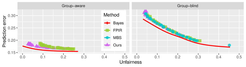
(a)

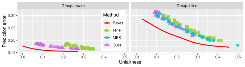
(b)

Figure 1: (a) The trade-off between prediction error and unfairness under (M1). The X-axis is the average unfairness measures $\bar{\mathcal{U}}_{\rm EOO}$ of the trained classifiers over 100 repetitions and the Y-axis is the average test prediction errors of these classifiers. The left and right panels correspond to the group-aware and group-blind scenarios, respectively. (b) As for (a) but the X-axis is the $95\%$ sample quantile ${\mathcal{U}}_{{\rm EOO},95}$ of the unfairness measures over 100 repetitions.

Although the cost of group-blindness in Remark 9 and the tradeoff in Remark 10 are in a minimax sense, we also observe similar phenomena in the specific simulation studies. Recall that the excess risk is the difference between the prediction error attained by the algorithm and that of the Bayes optimal classifier. In Figure 1(b), the group-aware and group-blind excess risks have comparable sizes when the unfairness level is large. Theoretically, they are the excess risk of the unconstrained classification problem in group-aware and group-blind scenarios, respectively. When the unfairness level decreases, the group-blind excess risk grows significantly, indicating the tradeoff between group-blind excess risk and the fairness constraint, while the group-aware excess risk has a relatively consistent magnitude. Finally, for small unfairness levels, the group-blind excess risk significantly exceeds the group-aware excess risk. This aligns with the cost of group-blindness, which is due to the error of predicting the sensitive attribute and the larger scale of $|\lambda^{*{\rm blind}}_{\alpha}|$ than $|\lambda^{*{\rm aware}}_{\alpha}|$ as verified by Figure 2.

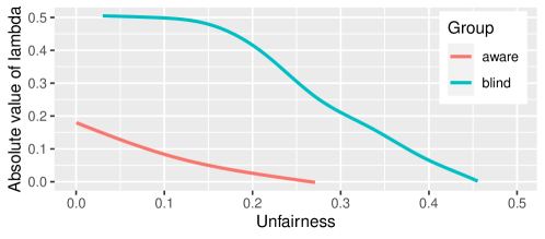
Figure 2: The curve of $|\lambda^{*G}_{\alpha}|$ on $\alpha$ under (M1). The red line is for the group-aware scenario and the cyan line is for the group-blind scenario.

5.2 Real Data Analysis

In this section, we apply the proposed algorithm to a real dataset, the Adult Census dataset (Asuncion and Newman, 2007), with 48842 instances. The target variable is whether each individual’s income is over $50000 or not. There are 14 non-sensitive covariates, including age, marriage status, education level, and other related information, while the sensitive attribute refers to gender. In this study, we randomly split the dataset into 16000 training samples, 16000 calibration samples, and 16842 test samples. The initial estimations are trained using the training data based on the same strategy as the simulation study, the fair classifier is constructed utilizing the calibration samples, and the test data is utilized to evaluate the prediction error and unfairness measure. Similar to the simulation study, we compare the proposed method with FPIR and MBS and repeat the procedure 100 times.

Due to the large sample size, we set $\alpha$ to be smaller as $\alpha\in\{0.04,0.06,0.08,0.10\}$ and choose $\delta=0.05$, then we report the prediction errors and unfairness measures for group-blind and group-aware scenarios in Table 3 and 4, respectively. The proposed method approximately controls the unfairness measures below $\alpha$ with probability $1-\delta$. However, FPIR and MBS can only control the unfairness on average, which may likely lead to unfair decisions in practice.

		$\alpha$
Methods		0.04	0.06	0.08	0.10
Ours	$\bar{\mathcal{U}}_{\rm EOO}$	0.026(0.017)	0.038(0.027)	0.052(0.028)	0.065(0.028)
	${\mathcal{U}}_{{\rm EOO},95}$	0.056	0.088	0.098	0.107
	Error	0.151(0.002)	0.151(0.002)	0.150(0.002)	0.150(0.002)
FPIR	$\bar{\mathcal{U}}_{\rm EOO}$	0.065(0.033)	0.080(0.031)	0.092(0.026)	0.091(0.024)
	${\mathcal{U}}_{{\rm EOO},95}$	0.118	0.127	0.132	0.131
	Error	0.150(0.002)	0.150(0.003)	0.150(0.002)	0.150(0.002)
MBS	$\bar{\mathcal{U}}_{\rm EOO}$	0.102(0.023)	0.099(0.026)	0.103(0.027)	0.093(0.023)
	${\mathcal{U}}_{{\rm EOO},95}$	0.138	0.145	0.149	0.131
	Error	0.149(0.002)	0.157(0.070)	0.157(0.070)	0.150(0.002)

Table 3: The unfairness measures and prediction errors of our method, FPIR, and MBS, respectively in the group-blind scenario on the Adult Census dataset. The notation is the same as Table 1

		$\alpha$
Methods		0.04	0.06	0.08	0.10
Ours	$\bar{\mathcal{U}}_{\rm EOO}$	0.026(0.017)	0.038(0.027)	0.052(0.028)	0.066(0.030)
	${\mathcal{U}}_{{\rm EOO},95}$	0.055	0.092	0.097	0.116
	Error	0.151(0.002)	0.151(0.002)	0.150(0.002)	0.150(0.002)
FPIR	$\bar{\mathcal{U}}_{\rm EOO}$	0.052(0.034)	0.073(0.035)	0.090(0.028)	0.090(0.029)
	${\mathcal{U}}_{{\rm EOO},95}$	0.114	0.130	0.132	0.138
	Error	0.150(0.002)	0.150(0.003)	0.150(0.002)	0.150(0.002)

Table 4: The unfairness measures and prediction errors of our method and FPIR, respectively in the group-aware scenario on the Adult Census dataset. The notation is the same as Table 1.

We also summarize the trade-off between the average prediction error and the average unfairness or the 95% sample quantile of the unfairness in Figure 3. In all cases, FPIR and MBS fail to achieve small unfairness levels and their curves are on the right of ours. Therefore, our method achieves better trade-off compared to FPIR and MBS.

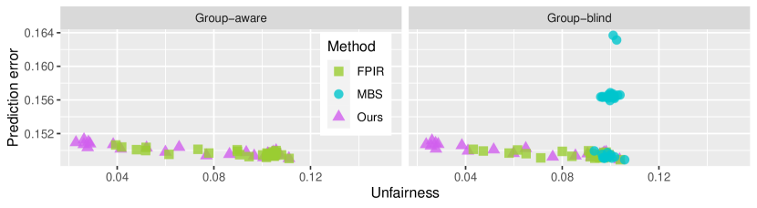
(a)

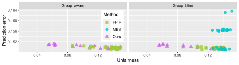
(b)

Figure 3: The trade-off between prediction error and unfairness on the Adult Census dataset. The display is the same as Figure 1.

6 Extensions

The previously discussed results can be extended in two directions. For binary sensitive attributes, the framework developed in Section 3 can be applied to other commonly used fairness notions. For multi-class sensitive attributes, we will also propose a unified framework with fairness and accuracy guarantees. However, for the brevity of the paper, in this section, we only derive the Bayes optimal $\alpha$-fair classifier with multi-class sensitive attributes. The application of Algorithm 1 to other fairness notions and the construction of the framework for multi-class sensitive attributes are deferred to Section A of the supplement (Hou and Zhang, 2024).

Similar to the binary sensitive attribute setting, most unfairness measures for multi-class sensitive attributes, as defined in Definition A.2 of the supplement (Hou and Zhang, 2024), can be rewritten as

$${\mathcal{U}}(f^{G})=\|{\mathbb{E}}\Phi^{G}(X,A)f^{G}(X,A)\|,$$

for some bounded vector-valued function $\Phi^{G}=(\phi^{G}_{k})_{k\in[\tilde{K}]}:{\mathbb{R}}^{d}\times[K]\rightarrow{\mathbb{R}}^{\tilde{K}}$, $\tilde{K}\in\mathbb{N}_{+}$ and norm $\|\cdot\|$ on ${\mathbb{R}}^{\tilde{K}}$, $G\in\{{\rm aware,blind}\}$. When $G={\rm blind}$, then $\Phi^{G}$ is only a function of $X$. Then we can characterize the solution of Problem (2) as follows.

Proposition 2 (Bayes Optimal $\alpha$-fair Classifier).

For $G\in\{{\rm aware,blind}\}$, the Bayes optimal classifier $f^{*G}_{\alpha}\in[0,1]^{{\mathbb{R}}^{d}\times[K]}$ of Problem (2) has the following form $P_{X,A}$-almost surely, with $P_{X,A}$ to be the joint distribution of $(X,A)$,

$$f^{*G}_{\alpha}(X,A)= {\mathbbm{1}}\big{(}g^{*G}_{\alpha}(X,A)>0\big{)}+b^{G}(X,A){\mathbbm{1}}\big{(}g^{*G}_{\alpha}(X,A)=0\big{)},$$

for

$$g^{*G}_{\alpha}(X,A)=2\eta^{G}(X,A)-1-\lambda^{*G\top}_{\alpha}\Phi^{G}(X,A),$$

$$\lambda^{*G}_{\alpha}\in\mathop{\rm arg\min}_{\lambda\in{\mathbb{R}}^{\tilde{K}}}{\mathbb{E}}\big{(}2\eta^{G}(X,A)-1-\lambda^{\top}\Phi^{G}(X,A)\big{)}_{+}+\alpha\|\lambda\|_{*},$$

and any $b^{G}\in[0,1]^{{\mathbb{R}}^{d}\times[K]}$ mapping from ${\mathbb{R}}^{d}\times[K]$ to $[0,1]$ such that $f^{*G}_{\alpha}$ satisfies the fairness constraint and

$$\lambda^{*G\top}_{\alpha}{\mathbb{E}}\Phi^{G}(X,A)f^{*G}_{\alpha}(X,A)=\|\lambda^{*G}_{\alpha}\|_{*}\|{\mathbb{E}}\Phi^{G}(X,A)f^{*G}_{\alpha}(X,A)\|=\|\lambda^{*G}_{\alpha}\|_{*}\alpha.$$ (20)

Here $\|\cdot\|_{*}$ is the dual norm of $\|\cdot\|$.

Remark 12.

Similar to binary sensitive attribute setting, $\|\lambda^{*G}_{\alpha}\|_{*}$ is always upper bounded. To see this, by Equation (20), we know

$$\|\lambda^{*G}_{\alpha}\|_{*}\alpha={\mathbb{E}}\lambda^{*G\top}_{\alpha}\Phi^{G}(X,A){\mathbbm{1}}\big{(}2\eta^{G}(X,A)-1>\lambda^{*G\top}_{\alpha}\Phi^{G}(X,A)\big{)}\leq{\mathbb{E}}\big{(}2\eta^{G}(X,A)-1\big{)}f^{*G}_{\alpha}(X,A)\leq 1,$$

therefore $\|\lambda^{*G}_{\alpha}\|_{*}\leq\alpha^{-1}$.

Similar to the case with binary sensitive attributes in Section 3, the Bayes optimal $\alpha$-fair classifier in Proposition 2 is a translation of the unconstrained Bayes optimal classifier ${\mathbbm{1}}(2\eta^{G}>1)$ by $\lambda^{*G\top}_{\alpha}\Phi^{G}$. This motivates us to construct a fair classifier by post-processing. See Section A.2 of the supplement (Hou and Zhang, 2024) for more details.

7 Discussion

In this work, we propose a comprehensive framework for fair classification with guaranteed fairness and excess risk for various fairness notions in both group-aware and group-blind scenarios. For binary sensitive attributes, we derive minimax lower bounds for the excess risks, which reveal the trade-off between group-blind excess risk and fairness, and uncover the cost of group-blindness. In the following, we point out some interesting directions for future work.

For binary sensitive attributes, we study the excess risk when ${\mathbbm{1}}(2\eta^{G}>1)$ is sufficiently fair or unfair. When ${\mathcal{U}}({\mathbbm{1}}(2\eta^{G}>1))$ is near $\alpha$, additional assumptions, such as those similar to the detection condition (Tong, 2013), are required to quantify the error of $\hat{\lambda}^{G}$. Then it would be interesting to derive a matching minimax lower bound, especially in the group-blind scenario.

For binary sensitive attributes, there is a gap $O_{P}(|\lambda^{*{\rm aware}}_{\alpha}|N^{-\frac{1}{2}})$ between the group-aware excess risk upper and lower bounds. We conjecture the upper bound is tight and new techniques may be required to prove the lower bound $O_{P}(|\lambda^{*{\rm aware}}_{\alpha}|N^{-\frac{1}{2}})$.

For the case with multi-class sensitive attributes studied in Section A.2 of the supplement (Hou and Zhang, 2024), we compare the prediction error of the proposed classifier $\hat{f}^{G}_{\hat{\lambda}_{\alpha}}$ with that of the Bayes optimal $\tilde{\alpha}$-fair classifier $f^{*G}_{\tilde{\alpha}}$ with a smaller unfairness level $\tilde{\alpha}\leq\alpha$. To compare with $f^{*G}_{\alpha}$, more complicated assumptions are required to control the error of $\hat{\lambda}^{G}_{\alpha}$. Then it would be interesting to define a more natural model space and characterize the minimax rate of the excess risk ${\mathcal{R}}(\hat{f}^{G})-{\mathcal{R}}(f^{*G}_{\alpha})$.

Supplement to “Finite-Sample and Distribution-Free Fair Classification: Optimal Trade-off Between Excess Risk and Fairness, and the Cost of Group-Blindness”

Appendix A Extensions

In this section, we build upon the previously discussed results by extending them in two directions. In Section A.1, we apply the framework proposed in Section 3 to more commonly used fairness notions. Then in Section A.2, we extend the framework to multi-class sensitive attributes.

A.1 Applications to More Fairness Notions

In this section, we apply the framework proposed in Section 3 to other widely used fairness notions defined in the following.

Definition 7 (Unfairness).

When $K=2$, for any randomized classifier $f$, the unfairness of $f$ in terms of

1. demographic parity (DP) is

   $${\mathcal{U}}_{\rm DP}(f)=|{\mathbb{P}}(Y_{f}(X,A)=1|A=1)-{\mathbb{P}}(Y_{f}(X,A)=1|A=2)|,$$

2. overall accuracy equality (OAE) is

   $${\mathcal{U}}_{\rm OAE}(f)= |{\mathbb{P}}(Y_{f}(X,A)=1|A=1,Y=1)+{\mathbb{P}}(Y_{f}(X,A)=0|A=1,Y=0)$$

   $$-{\mathbb{P}}(Y_{f}(X,A)=1|A=2,Y=1)-{\mathbb{P}}(Y_{f}(X,A)=0|A=2,Y=0)|,$$

3. predictive equality (PE) is

   $${\mathcal{U}}_{\rm PE}(f)=|{\mathbb{P}}(Y_{f}(X,A)=1|A=1,Y=0)-{\mathbb{P}}(Y_{f}(X,A)=1|A=2,Y=0)|.$$

Another commonly used fairness notion is equalized odds as defined in Definition 8. However, since the unfairness measure corresponding to equalized odds can not be reduced in this way to the absolute value of a linear combination of conditional expectations, we treat it as the multi-class sensitive attribute case and address it in Section A.2.

Recall that $\rho_{a}(X)={\mathbb{P}}(A=a|X)$, $p_{a}={\mathbb{P}}(A=a)$. To apply Algorithm 1 to unfairness measures in Definition 7, we specify the corresponding $\phi^{G}_{F}$ for $G\in\{{\rm aware,blind}\},F\in\{{\rm DP,OAE,PE}\}$ in Table 5. Here $G$ indicates the group-aware or group-blind scenarios and $F$ specifies the fairness notions: demographic parity (DP), overall accuracy equality (OAE), or predictive equality (PE).

$F$	$G={\rm aware}$	$G={\rm blind}$
DP	$\frac{3-2a}{p_{a}}$	$\frac{\rho_{1}(x)-p_{1}}{p_{1}p_{2}}$
OAE	$\frac{3-2a}{p_{1,a}p_{0,a}}(p_{a}\eta^{G}(x,a)-p_{1,a})$	$\sum_{a\in[2],y\in\{0,1\}}\frac{\rho_{a|y}(x)(\eta^{G}(x,a)+y-1)}{(3-2a)p_{y,a}}$
PE	$\frac{3-2a}{p_{0,a}}(1-\eta^{G}(x,a))$	$\frac{(1-p_{Y})\rho_{1|0}(x)-p_{0,1}}{p_{0,1}p_{0,2}}(1-\eta^{G}(x,a))$

Table 5: The form of $\phi^{G}_{F}(x,a)$ for $G\in\{{\rm aware,blind}\},F\in\{{\rm DP,OAE,PE}\}$.

We have ${\mathcal{U}}_{F}(f^{G})=|{\mathbb{E}}\phi_{F}^{G}(X,A)f^{G}(X,A)|$ for $F\in\{{\rm DP,OAE,PE}\}$. Similar to Section 4.1 and 4.2, we impose the Hölder smoothness, observability assumptions, and strong density assumption 6.

Assumption 10 (Hölder Smoothness).

We assume $\eta^{G}(\cdot,a)\in{\mathcal{H}}(\beta_{Y},L_{Y})$, $\rho_{1},\rho_{1|y}\in{\mathcal{H}}(\beta_{A},L_{A})$ for all $G\in\{{\rm aware,blind}\},a\in[2],y\in\{0,1\}$.

Assumption 11 (Observability).

We assume the existence of constants $c_{5}>0$ such that $p_{y,a}>c_{5}$ for all $y\in\{0,1\},a\in[2]$.

Following the same strategy as Section 4 to estimate $\eta^{G}$ and $\phi^{G}_{F}$ on $\tilde{\mathcal{D}}$, we denote $\epsilon_{\eta}\asymp\big{(}\frac{d\log\tilde{n}+\log\frac{1}{\delta_{\rm init}}}{\tilde{n}}\big{)}^{\frac{\beta_{Y}}{2\beta_{Y}+d}}$ and choose $\epsilon_{\phi,F}^{G}$ and $\epsilon_{\alpha,F}$ in Table 6 and Table 7, respectively. Here the value of $\epsilon_{\alpha,F}$ only depends on the fairness notions and remains the same across both group-aware and group-blind scenarios.

$F$	$G={\rm aware}$	$G={\rm blind}$
DP	$\sqrt{\frac{\log\frac{1}{\delta_{\rm init}}}{\tilde{n}}}$	$\big{(}\frac{d\log\tilde{n}+\log\frac{1}{\delta_{\rm init}}}{\tilde{n}}\big{)}^{\frac{\beta_{A}}{2\beta_{A}+d}}$
OAE, PE	$\big{(}\frac{d\log\tilde{n}+\log\frac{1}{\delta_{\rm init}}}{\tilde{n}}\big{)}^{\frac{\beta_{Y}}{2\beta_{Y}+d}}$	$\big{(}\frac{d\log\tilde{n}+\log\frac{1}{\delta_{\rm init}}}{\tilde{n}}\big{)}^{\frac{\beta_{Y}}{2\beta_{Y}+d}}+\big{(}\frac{d\log\tilde{n}+\log\frac{1}{\delta_{\rm init}}}{\tilde{n}}\big{)}^{\frac{\beta_{A}}{2\beta_{A}+d}}$

Table 6: The order of $\epsilon_{\phi,F}^{G}$ for $G\in\{{\rm aware,blind}\},F\in\{{\rm DP,OAE,PE}\}$.

$F$	$\epsilon_{\alpha,F}$
DP	$\sum_{a\in[2]}\big{(}72\sqrt{\frac{2\log 4e^{2}}{n_{a}}}+\sqrt{\frac{1}{2n_{a}}\log\frac{4}{\delta_{\rm post}}}\big{)}$
OAE	$\sum_{a\in[2],y\in\{0,1\}}\big{(}72\sqrt{\frac{2\log 4e^{2}}{n_{y,a}}}+\sqrt{\frac{1}{2n_{y,a}}\log\frac{8}{\delta_{\rm post}}}\big{)}$
PE	$\sum_{a\in[2]}\big{(}72\sqrt{\frac{2\log 4e^{2}}{n_{0,a}}}+\sqrt{\frac{1}{2n_{0,a}}\log\frac{4}{\delta_{\rm post}}}\big{)}$

Table 7: The value of $\epsilon_{\alpha,F}$ for $F\in\{{\rm DP,OAE,PE}\}$.

Then we can guarantee the performance of the classifier $\hat{f}^{G}_{\alpha,F}$ produced by Algorithm 1.

Corollary 3 (Excess Risk Upper Bound).

For $G\in\{{\rm aware,blind}\},F\in\{{\rm DP,OAE,PE}\}$, suppose Assumptions 6, 10 and 11 hold.

1. With probability at least $1-\delta$, for any $\alpha\geq(3\epsilon_{\alpha,F}+2\tilde{\epsilon}_{\eta}^{G})\vee(2\epsilon_{\alpha,F}+M_{\phi,F}^{G})$, Algorithm 1 has a unique output $\hat{f}^{G}_{\alpha,F}$ and it satisfies ${\mathcal{U}}_{F}(\hat{f}^{G}_{\alpha,F})\leq\alpha$.

2. Under Assumptions 2, 3 and 4, if the unfairness difference $D_{0}$ satisfies

   $$D_{0}\leq-2\epsilon_{\alpha,F}-\tilde{\epsilon}_{\eta}^{G}\quad{\rm or}\quad D_{0}>\tilde{\epsilon}_{\eta}^{G}\vee c_{3}\big{(}2\epsilon_{\alpha,F}+\frac{c_{1}}{c_{5}}(2\epsilon_{\alpha,F}+(1+2c_{4})|\lambda^{*G}_{\alpha,F}|\epsilon_{\phi,F}^{G})^{\gamma}\big{)},$$

   then with probability at least $1-\delta$, for any $\alpha$ defined in part 1), we have

   $${\mathcal{R}}(\hat{f}^{G}_{\alpha,F})-{\mathcal{R}}(f^{*G}_{\alpha,F})\lesssim|\lambda^{*G}_{\alpha,F}|\epsilon_{\alpha,F}+\epsilon_{\eta}^{1+\gamma}+\big{(}|\lambda^{*G}_{\alpha,F}|\epsilon_{\phi,F}^{G}\big{)}^{1+\gamma}.$$ (21)

A.2 A Unified Framework for Multi-Class Sensitive Attribute

In this section, we provide a general post-processing algorithm and excess risk analysis for fair classification. First, we define the unfairness measures for multi-class sensitive attributes.

Definition 8 (Unfairness).

For any randomized classifier $f$, the unfairness of $f$ in terms of

1. demographic parity is

   $${\mathcal{U}}_{\rm DP}(f)=\max_{a\in[K]}|{\mathbb{P}}(Y_{f}(X,A)=1|A=a)-{\mathbb{P}}(Y_{f}(X,A)=1)|,$$

2. equalized odds is

   $${\mathcal{U}}_{\rm EO}(f)=\max_{a\in[K]}\big{\{} |{\mathbb{P}}(Y_{f}(X,A)=1|A=a,Y=1)-{\mathbb{P}}(Y_{f}(X,A)=1|Y=1)|$$

   $$\vee|{\mathbb{P}}(Y_{f}(X,A)=0|A=a,Y=0)-{\mathbb{P}}(Y_{f}(X,A)=0|Y=0)|\big{\}},$$

3. equality of opportunity is

   $${\mathcal{U}}_{\rm EOO}(f)=\max_{a\in[K]}|{\mathbb{P}}(Y_{f}(X,A)=1|A=a,Y=1)-{\mathbb{P}}(Y_{f}(X,A)=1|Y=1)|,$$

4. overall accuracy equality is

   $${\mathcal{U}}_{\rm OAE}(f)=\max_{a\in[K]}\big{|} {\mathbb{P}}(Y_{f}(X,A)=1|A=a,Y=1)+{\mathbb{P}}(Y_{f}(X,A)=0|A=a,Y=0)$$

   $$-{\mathbb{P}}(Y_{f}(X,A)=1|Y=1)-{\mathbb{P}}(Y_{f}(X,A)=0|Y=0)\big{|},$$

5. predictive equality is

   $${\mathcal{U}}_{\rm PE}(f)=\max_{a\in[K]}|{\mathbb{P}}(Y_{f}(X,A)=1|A=a,Y=0)-{\mathbb{P}}(Y_{f}(X,A)=1|Y=0)|.$$

A.2.1 Post-processing Algorithm

In this section, we propose a general algorithm for various fairness notions with fairness and excess risk guarantee. For the unfairness measures in Definition 8, the vector norms $\|\cdot\|$ and $\|\cdot\|_{*}$ in Proposition 2 equal to the $\ell_{\infty}$ norm $\|\cdot\|_{\infty}$ and $\ell_{1}$ norm $\|\cdot\|_{1}$, respectively.

It is clear that for the same $\tilde{K}$ defined above, the unfairness measures in Definition 8 can also be rewritten as

$${\mathcal{U}}(f^{G})=\max_{k\in[\tilde{K}]}\bigg{|}\sum_{j\in[m]}\kappa_{j}{\mathbb{E}}_{kj}f^{G}(X,A)\bigg{|},$$

with $\{\kappa_{j}\in{\mathbb{R}}:j\in[m]\}$ are known coefficients and $\{{\mathbb{E}}_{kj}:k\in[\tilde{K}],j\in[m]\}$ are a set of conditional expectations given the sensitive attributes, depending on the fairness notions.

Similar to the binary sensitive attribute case in Section 3.2, we assume the initial estimators $\hat{\eta}^{G}$ and $\hat{\Phi}^{G}$ are given and independent of the dataset ${\mathcal{D}}$. We select $\hat{\lambda}$ based on ${\mathcal{D}}$ to post-process $\hat{\eta}^{G}$ and $\hat{\Phi}^{G}$. Denote

$$\hat{f}^{G}_{\lambda}(x,a)={\mathbbm{1}}\big{(}2\hat{\eta}^{G}(x,a)-1>\lambda^{\top}\hat{\Phi}^{G}(x,a)\big{)},$$

the excess risk of $\hat{f}^{G}_{\lambda}$ can be decomposed as

$${\mathcal{R}}(\hat{f}^{G}_{\lambda})-{\mathcal{R}}(f^{*G}_{\alpha})$$

$$= \underbrace{{\mathbb{E}}|g^{*G}_{\alpha}(X,A)||f^{*G}_{\alpha}(X,A)-\hat{f}^{G}_{\lambda}(X,A)|}_{T_{1}}+\underbrace{{\mathbb{E}}\lambda^{*G\top}_{\alpha}\Phi^{G}(X,A)\big{(}f^{*G}_{\alpha}(X,A)-\hat{f}^{G}_{\lambda}(X,A)\big{)}}_{T_{2}}.$$

For the binary sensitive attribute case in Section 3.2, $\lambda^{*G}_{\alpha}$ is a real number with two well-separated directions, i.e. positive or negative. Then as long as $\alpha$ is large enough, we are able to construct $\hat{\lambda}$ as in Algorithm 1 such that it roughly maximizes ${\rm sgn}(\lambda^{*G}_{\alpha}){\mathbb{E}}\phi^{G}(X,A)\hat{f}^{G}_{\lambda}(X,A)$, or equivalently minimizes $T_{2}$, and ensures ${\mathcal{U}}(\hat{f}^{G}_{\lambda})=\max_{s\in\{1,-1\}}{\mathbb{E}}s\phi^{G}(X,A)\hat{f}^{G}_{\lambda}(X,A)\leq\alpha$ simultaneously. However, for multi-class sensitive attributes, $\lambda^{*G}_{\alpha}$ has dimension $\tilde{K}>1$ and there are continuum directions $\{\mu\in{\mathbb{R}}^{\tilde{K}}:\|\mu\|_{1}=1\}$. Then it is not clear how to directly control $\frac{\lambda^{*G\top}_{\alpha}}{\|\lambda^{*G}_{\alpha}\|_{1}}{\mathbb{E}}\Phi^{G}(X,A)\hat{f}^{G}_{\lambda}(X,A)$ and ${\mathcal{U}}(\hat{f}^{G}_{\lambda})=\sup_{\|\mu\|_{1}=1}\mu^{\top}{\mathbb{E}}\Phi^{G}(X,A)\hat{f}^{G}_{\lambda}(X,A)$ simultaneously. Consequently, the strategy in Algorithms 1 can not be applied in this case. In the following, we propose an algorithm to select $\lambda$ using empirical risk minimization.

Denote the empirical unfairness as

$$\hat{\mathcal{U}}(f^{G})=\max_{k\in[\tilde{K}]}\bigg{|}\sum_{j\in[m]}\kappa_{j}\hat{\mathbb{E}}_{kj}f^{G}(X,A)\bigg{|}$$

with $\{\hat{\mathbb{E}}_{kj}:k\in[\tilde{K}],j\in[m]\}$ to be the set of conditional sample averages corresponding to $\{{\mathbb{E}}_{kj}:k\in[\tilde{K}],j\in[m]\}$ based on data ${\mathcal{D}}$. We denote $n_{(kj)}$ to be the number of samples in ${\mathcal{D}}$ used to calculate the conditional sample average $\hat{\mathbb{E}}_{kj}$, and set

$$\epsilon_{\alpha}=\max_{k\in[\tilde{K}]}\sum_{j\in[m]}|\kappa_{j}|\bigg{\{}72\sqrt{\frac{(\tilde{K}+1)\log 4e^{2}}{n_{(kj)}}}+\sqrt{\frac{1}{2n_{(kj)}}\log\frac{2\tilde{K}m}{\delta_{\rm post}}}\bigg{\}}.$$

Then the following lemma ensures the possibility of distribution-free and finite-sample fairness control.

Lemma 6.

With probability at least $1-\delta_{\rm post}$ on ${\mathcal{D}}$,

$$\sup_{\lambda\in{\mathbb{R}}^{\tilde{K}}}|\hat{\mathcal{U}}(\hat{f}^{G}_{\lambda})-{\mathcal{U}}(\hat{f}^{G}_{\lambda})|\leq\epsilon_{\alpha}.$$

Following Lemma 6, we estimate $\lambda^{*G}_{\alpha}$ by

$$\hat{\lambda}^{G}_{\alpha}\in\mathop{\rm arg\min}_{\lambda\in{\mathbb{R}}^{\tilde{K}}}\sum_{i=1}^{n}{\mathbbm{1}}\big{(}Y_{i}\neq\hat{f}^{G}_{\lambda}(X_{i},A_{i})\big{)}\quad{\rm s.t.}\quad\hat{\mathcal{U}}(\hat{f}^{G}_{\lambda})\leq\alpha-\epsilon_{\alpha},$$ (22)

and set the classifier as $\hat{f}^{G}_{\hat{\lambda}_{\alpha}}$. We summarize the above procedures in Algorithm 2.

Algorithm 2 Post-processing with Multi-Class Sensitive Attribute

Input: Data ${\mathcal{D}}$, the initial estimators $\hat{\eta}^{G},\hat{\Phi}^{G}$, the unfairness level $\alpha$, the tolerance $\delta$, and the scenario $G\in\{{\rm aware,blind}\}$.

Output: $\hat{f}^{G}_{\hat{\lambda}}$.

Step 1: Solve

$$\hat{\lambda}^{G}_{\alpha}\in\mathop{\rm arg\min}_{\lambda\in{\mathbb{R}}^{\tilde{K}}}\sum_{i=1}^{n}{\mathbbm{1}}\big{(}Y_{i}\neq\hat{f}^{G}_{\lambda}(X_{i},A_{i})\big{)}\quad{\rm s.t.}\quad\hat{\mathcal{U}}(\hat{f}^{G}_{\lambda})\leq\alpha-\epsilon_{\alpha}.$$

Step 2: Output $\hat{f}^{G}_{\hat{\lambda}_{\alpha}}(x,a)={\mathbbm{1}}\big{(}2\hat{\eta}^{G}(x,a)-1>\hat{\lambda}^{G\top}_{\alpha}\hat{\Phi}^{G}(x,a)\big{)}$.

A.2.2 Performance Guarantee

To study the performance of the proposed algorithm, we denote $\epsilon_{\eta}$ and $\epsilon_{\phi}$ to be the estimation errors of $\hat{\eta}^{G}$ and $\hat{\Phi}^{G}$ respectively,

$$\|\hat{\eta}^{G}-\eta^{G}\|_{\infty}\leq\epsilon_{\eta},\quad\max_{k\in[\tilde{K}]}\|\hat{\phi}_{k}^{G}-\phi_{k}^{G}\|_{\infty}\leq\epsilon_{\phi}.$$

For $\tilde{\epsilon}_{\alpha}$ to be specified later, we denote $\tilde{\alpha}=\alpha-\tilde{\epsilon}_{\alpha}$ and denote the Bayes optimal $\tilde{\alpha}$-fair classifier as

$$\lambda^{*G}_{\tilde{\alpha}}\in\mathop{\rm arg\min}_{\lambda\in{\mathbb{R}}^{\tilde{K}}}{\mathbb{E}}\big{(}2\eta^{G}(X,A)-1-\lambda^{\top}\Phi^{G}(X,A)\big{)}_{+}+\tilde{\alpha}\|\lambda\|_{1},$$

$$f^{*G}_{\tilde{\alpha}}(x,a)={\mathbbm{1}}\big{(}g^{*G}_{\tilde{\alpha}}(x,a)>0),\quad g^{*G}_{\tilde{\alpha}}(x,a)=2\eta^{G}(x,a)-1-\lambda^{*G\top}_{\tilde{\alpha}}\Phi^{G}(x,a).$$

Then we denote the margins $\tilde{\epsilon}_{\eta}^{G}$ and $\tilde{\epsilon}_{g,\tilde{\alpha}}^{G}$ of $2\eta^{G}-1$ and $g^{*G}_{\tilde{\alpha}}$ as

$$\tilde{\epsilon}_{\eta}^{G}=\max_{k\in[\tilde{K}]}{\mathbb{E}}|\phi_{k}^{G}(X,A)|{\mathbbm{1}}(|2\eta^{G}(X,A)-1|\leq 2\epsilon_{\eta}),$$

$$\tilde{\epsilon}_{g,\tilde{\alpha}}^{G}=\max_{k\in[\tilde{K}]}{\mathbb{E}}|\phi^{G}_{k}(X,A)|{\mathbbm{1}}\big{(}|g^{*G}_{\tilde{\alpha}}(X,A)|\leq 2\epsilon_{\eta}+\|\lambda^{*G}_{\tilde{\alpha}}\|_{1}\epsilon_{\phi}\big{)}.$$

$\tilde{\epsilon}_{\eta}^{G}$ and $\tilde{\epsilon}_{g,\tilde{\alpha}}^{G}$ measure the mass of $2\eta^{G}(X,A)-1$ and $g^{*G}_{\tilde{\alpha}}(X,A)$ around 0, respectively. Since $\Phi^{G}$ is bounded and $\epsilon_{\eta}$, $\epsilon_{\phi}$ are typically small, we know $\tilde{\epsilon}_{\eta}^{G}$ and $\tilde{\epsilon}_{g,\tilde{\alpha}}^{G}$ are small as long as $2\eta^{G}-1$ and $g^{*G}_{\tilde{\alpha}}$ are not too concentrated around 0.

Similar to the binary sensitive attribute case, we denote $D_{0}={\mathcal{U}}({\mathbbm{1}}(2\eta^{G}>1))-\alpha$ to be the difference between the unfairness of the unconstrained Bayes optimal classifier ${\mathbbm{1}}(2\eta^{G}>1)$ and the specified unfairness level $\alpha$. If $D_{0}\leq 0$, we know $f^{*G}_{\alpha}={\mathbbm{1}}(2\eta^{G}>1)$ and $\lambda^{*}_{\alpha}=0$. If $D_{0}>0$, ${\mathbbm{1}}(2\eta^{G}>1)$ is not $\alpha$-fair and need to be adjusted by $\lambda^{*G\top}_{\alpha}\Phi^{G}$.

Now we specify the choice of $\tilde{\epsilon}_{\alpha}$ as follows.

1. If $D_{0}\leq-\tilde{\epsilon}_{\eta}^{G}-2\epsilon_{\alpha}$, we set $\tilde{\epsilon}_{\alpha}=0$.

2. If $D_{0}>-\tilde{\epsilon}_{\eta}^{G}-2\epsilon_{\alpha}$, we choose $\tilde{\epsilon}_{\alpha}$ such that

   $$\tilde{\epsilon}_{\alpha}\geq 2\epsilon_{\alpha}+\tilde{\epsilon}_{g,\tilde{\alpha}}^{G}.$$ (23)

Therefore, when $D_{0}\leq-\tilde{\epsilon}_{\eta}^{G}-2\epsilon_{\alpha}$, we have $\tilde{\alpha}=\alpha$ and $\lambda^{*}_{\tilde{\alpha}}=\lambda^{*}_{\alpha}=0$.

Remark 13.

Now we give an example where Equation (23) is satisfied. Suppose the density of $2\eta^{G}(X,A)-1-\lambda^{\top}\Phi^{G}(X,A)$ is upper bounded for all $\lambda\in{\mathbb{R}}^{\tilde{K}}$. Since $\phi^{G}_{k}$, $k\in[\tilde{K}]$ are bounded, we have $\tilde{\epsilon}_{g,\tilde{\alpha}}^{G}\leq c\epsilon_{\eta}+c\|\lambda^{*G}_{\tilde{\alpha}}\|_{1}\epsilon_{\phi}$. Using the naive upper bound in Remark 12, we get $\|\lambda^{*}_{\tilde{\alpha}}\|_{1}\leq(\alpha-\tilde{\epsilon}_{\alpha})^{-1}$. When $\alpha\geq 4\epsilon_{\alpha}+2c\epsilon_{\eta}+2\sqrt{2c\epsilon_{\phi}}$, condition (23) is satisfied for $\tilde{\epsilon}_{\alpha}=2\epsilon_{\alpha}+c\epsilon_{\eta}+\sqrt{2c\epsilon_{\phi}}$.

Similar to Section 3.2, we make the margin assumption (Tsybakov, 2004).

Assumption 12 (Margin Assumption).

There exist $\tilde{\gamma}\geq 0$ and constant $c_{1}>0$ such that for any $\epsilon\geq 0$, we have

$${\mathbb{P}}\big{(}|g^{*G}_{\tilde{\alpha}}(X,A)|\leq\epsilon\big{)}\leq c_{1}\epsilon^{\tilde{\gamma}}.$$

Note that the margin assumption 12 is on $g^{*G}_{\tilde{\alpha}}$, not $g^{*G}_{\alpha}$. To clarify the rationale behind this choice, we first present the following theorem, which controls the fairness and excess risk.

Theorem 5.

1. With probability at least $1-\delta_{\rm post}$, for any $\alpha\geq\tilde{\epsilon}_{\alpha}$, we have Algorithm 2 to be feasible and ${\mathcal{U}}(\hat{f}^{G}_{\hat{\lambda}_{\alpha}})\leq\alpha$.

2. Under Assumption 12, we have with probability at least $1-2\delta_{\rm post}$, for any $\alpha\geq\tilde{\epsilon}_{\alpha}$,

   $${\mathcal{R}}(\hat{f}^{G}_{\hat{\lambda}_{\alpha}})-{\mathcal{R}}(f^{*G}_{\tilde{\alpha}})\lesssim\|\lambda^{*G}_{\tilde{\alpha}}\|_{1}\tilde{\epsilon}_{\alpha}+\big{(}\epsilon_{\eta}+\|\lambda^{*G}_{\tilde{\alpha}}\|_{1}\epsilon_{\phi}\big{)}^{1+\tilde{\gamma}}+\bigg{(}\frac{\tilde{K}\log n+\log\frac{1}{\delta_{\rm post}}}{n}\bigg{)}^{\frac{1+\tilde{\gamma}}{2+\tilde{\gamma}}}.$$ (24)

In Theorem 5, we compare the prediction error of $\hat{f}^{G}_{\hat{\lambda}_{\alpha}}$ with that of $f^{*G}_{\tilde{\alpha}}$, rather than $f^{*G}_{\alpha}$. So ${\mathcal{R}}(\hat{f}^{G}_{\hat{\lambda}_{\alpha}})-{\mathcal{R}}(f^{*G}_{\tilde{\alpha}})$ may not always be non-negative. To explain this, note that $\hat{f}^{G}_{\lambda^{*}_{\alpha}}$ may not satisfy the constraint $\hat{\mathcal{U}}(\hat{f}^{G}_{\lambda^{*}_{\alpha}})\leq\alpha-\epsilon_{\alpha}$, therefore we have to select another $\lambda$ that meets the empirical fairness constraint $\hat{\mathcal{U}}(\hat{f}^{G}_{\lambda})\leq\alpha-\epsilon_{\alpha}$ and exhibits satisfactory prediction performance. $\lambda^{*}_{\tilde{\alpha}}$ turns out to satisfy both conditions. However, when comparing with $f^{*G}_{\alpha}$, it is imperative to control the distance between $\lambda^{*}_{\tilde{\alpha}}$ and $\lambda^{*}_{\alpha}$, necessitating additional assumptions such as those similar to the detection assumption (Tong, 2013) in the context of Neyman-Pearson classification. Consequently, to maintain the simplicity of our results with the fewest assumptions, we articulate the excess risk comparing with $f^{*G}_{\tilde{\alpha}}$. Then the margin assumption 12 is also on $g^{*G}_{\tilde{\alpha}}$ instead of $g^{*G}_{\alpha}$.

Under the $\beta_{Y}$-Hölder smoothness assumption on $\eta^{G}$, if we estimate $\eta^{G}$ on an independent dataset $\tilde{\mathcal{D}}$ with sample size $\tilde{n}$, we know $\epsilon_{\eta}\asymp(\frac{d\log\tilde{n}}{\tilde{n}})^{\frac{\beta_{Y}}{2\beta_{Y}+d}}$. When $n\gtrsim\tilde{n}$, under the standard condition $\beta_{Y}\tilde{\gamma}\leq d$ (Audibert and Tsybakov, 2007), with $d\gtrsim\tilde{K}$, we have $(\frac{\tilde{K}\log n}{n})^{\frac{1+\tilde{\gamma}}{2+\tilde{\gamma}}}\lesssim\epsilon_{\eta}^{1+\tilde{\gamma}}$. Then the excess risk (24) becomes $O_{P}\big{(}\|\lambda^{*}_{\tilde{\alpha}}\|_{1}\tilde{\epsilon}_{\alpha}+\big{(}\epsilon_{\eta}+\|\lambda^{*}_{\tilde{\alpha}}\epsilon_{\phi}\|\big{)}^{1+\tilde{\gamma}}\big{)}$, sharing the same form as the excess risk (8) with binary sensitive attributes. If ${\mathbbm{1}}(2\eta^{G}>1)$ is already $\tilde{\alpha}$-fair, we know $\lambda^{*}_{\tilde{\alpha}}=\lambda^{*}_{\alpha}=0$. Then the excess risk (24) becomes $O_{P}(\epsilon_{\eta}^{1+\tilde{\gamma}})$, which is minimax optimal up to logarithmic factors (Audibert and Tsybakov, 2007). When ${\mathbbm{1}}(2\eta^{G}>1)$ is not $\tilde{\alpha}$-fair, we know $\lambda^{*}_{\tilde{\alpha}}\neq 0$. Then we incur an additional cost $O_{P}\big{(}\|\lambda^{*G}_{\tilde{\alpha}}\|_{1}\tilde{\epsilon}_{\alpha}+(\|\lambda^{*G}_{\tilde{\alpha}}\|_{1}\epsilon_{\phi})^{1+\tilde{\gamma}}\big{)}$ due to the fairness constraint.

Appendix B Supplementary Simulation Results

In this section, we present the omitted simulation results for (M2) and (M3). The results and interpretations are similar to those of (M1), therefore we report the results without explanations.

		$\alpha$
Methods		0.08	0.11	0.14	0.17	0.20
Ours	$\bar{\mathcal{U}}_{\rm EOO}$	0.055(0.042)	0.055(0.039)	0.061(0.044)	0.086(0.053)	0.100(0.057)
	${\mathcal{U}}_{{\rm EOO},95}$	0.137	0.134	0.137	0.173	0.184
	Error	0.318(0.027)	0.319(0.026)	0.308(0.024)	0.297(0.018)	0.295(0.018)
FPIR	$\bar{\mathcal{U}}_{\rm EOO}$	0.084(0.051)	0.120(0.050)	0.135(0.052)	0.148(0.049)	0.160(0.045)
	${\mathcal{U}}_{{\rm EOO},95}$	0.179	0.195	0.206	0.223	0.225
	Error	0.296(0.017)	0.289(0.013)	0.285(0.010)	0.284(0.010)	0.283(0.008)
MBS	$\bar{\mathcal{U}}_{\rm EOO}$	0.082(0.058)	0.099(0.056)	0.116(0.060)	0.126(0.056)	0.140(0.061)
	${\mathcal{U}}_{{\rm EOO},95}$	0.178	0.183	0.222	0.229	0.239
	Error	0.297(0.017)	0.293(0.016)	0.290(0.014)	0.286(0.010)	0.286(0.010)
Bayes	Error	0.283	0.276	0.272	0.272	0.272

Table 8: The unfairness measures and prediction errors of our method, FPIR, and MBS, respectively in the group-blind scenario under (M2). And the prediction errors of Bayes optimal fair classifiers. $\bar{\mathcal{U}}_{\rm EOO}$ is the average unfairness over 100 repetitions. ${\mathcal{U}}_{{\rm EOO},95}$ is the $95\%$ sample quantile of the unfairness measures produced by 100 repetitions. Error is the average prediction error.

		$\alpha$
Methods		0.08	0.11	0.14	0.17	0.20
Ours	$\bar{\mathcal{U}}_{\rm EOO}$	0.051(0.041)	0.047(0.035)	0.063(0.049)	0.074(0.050)	0.088(0.062)
	${\mathcal{U}}_{{\rm EOO},95}$	0.121	0.114	0.157	0.171	0.198
	Error	0.266(0.010)	0.267(0.009)	0.264(0.009)	0.262(0.009)	0.262(0.007)
FPIR	$\bar{\mathcal{U}}_{\rm EOO}$	0.126(0.077)	0.130(0.079)	0.135(0.083)	0.151(0.081)	0.172(0.084)
	${\mathcal{U}}_{{\rm EOO},95}$	0.262	0.262	0.266	0.265	0.288
	Error	0.264(0.015)	0.262(0.010)	0.261(0.010)	0.259(0.010)	0.260(0.007)
Bayes	Error	0.245	0.245	0.244	0.243	0.243

Table 9: The unfairness measures and prediction errors of our method and FPIR, respectively in the group-aware scenario under (M2). The notation is the same as Table 8.

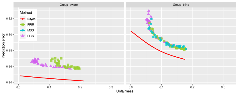
(a)

(b)

Figure 4: (a) The trade-off between prediction error and unfairness under (M2). The X-axis is the average unfairness measures $\bar{\mathcal{U}}_{\rm EOO}$ of the trained classifiers over 100 repetitions and the Y-axis is the average test prediction errors of these classifiers. The left and right panels correspond to the group-aware and group-blind scenarios, respectively. (b) As for (a) but the X-axis is the $95\%$ sample quantile ${\mathcal{U}}_{{\rm EOO},95}$ of the unfairness measures over 100 repetitions.

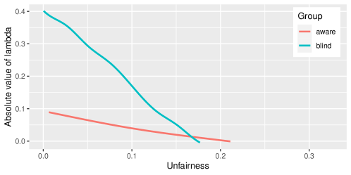
Figure 5: The curve of $|\lambda^{*G}_{\alpha}|$ on $\alpha$ under (M2). The red line is for the group-aware scenario and the cyan line is for the group-blind scenario.

		$\alpha$
Methods		0.08	0.11	0.14	0.17	0.20
Ours	$\bar{\mathcal{U}}_{\rm EOO}$	0.039(0.033)	0.051(0.038)	0.074(0.044)	0.098(0.048)	0.138(0.048)
	${\mathcal{U}}_{{\rm EOO},95}$	0.107	0.128	0.143	0.180	0.216
	Error	0.333(0.024)	0.320(0.024)	0.306(0.025)	0.294(0.023)	0.273(0.023)
FPIR	$\bar{\mathcal{U}}_{\rm EOO}$	0.101(0.061)	0.124(0.054)	0.157(0.066)	0.178(0.056)	0.209(0.069)
	${\mathcal{U}}_{{\rm EOO},95}$	0.211	0.210	0.271	0.271	0.313
	Error	0.293(0.030)	0.279(0.027)	0.266(0.029)	0.258(0.022)	0.245(0.026)
MBS	$\bar{\mathcal{U}}_{\rm EOO}$	0.088(0.043)	0.109(0.048)	0.140(0.053)	0.172(0.047)	0.211(0.048)
	${\mathcal{U}}_{{\rm EOO},95}$	0.148	0.181	0.214	0.247	0.282
	Error	0.299(0.023)	0.285(0.023)	0.273(0.025)	0.260(0.021)	0.243(0.018)
Bayes	Error	0.265	0.251	0.238	0.226	0.214

Table 10: The unfairness measures and prediction errors of our method, FPIR, and MBS, respectively in the group-blind scenario under (M3). And the prediction errors of Bayes optimal fair classifiers. $\bar{\mathcal{U}}_{\rm EOO}$ is the average unfairness over 100 repetitions. ${\mathcal{U}}_{{\rm EOO},95}$ is the $95\%$ sample quantile of the unfairness measures produced by 100 repetitions. Error is the average prediction error.

		$\alpha$
Methods		0.08	0.11	0.14	0.17	0.20
Ours	$\bar{\mathcal{U}}_{\rm EOO}$	0.036(0.027)	0.045(0.033)	0.067(0.040)	0.103(0.043)	0.132(0.046)
	${\mathcal{U}}_{{\rm EOO},95}$	0.091	0.105	0.145	0.170	0.213
	Error	0.209(0.011)	0.206(0.009)	0.202(0.008)	0.199(0.008)	0.194(0.008)
FPIR	$\bar{\mathcal{U}}_{\rm EOO}$	0.103(0.084)	0.112(0.075)	0.136(0.091)	0.147(0.078)	0.190(0.102)
	${\mathcal{U}}_{{\rm EOO},95}$	0.269	0.249	0.305	0.295	0.360
	Error	0.206(0.019)	0.201(0.016)	0.197(0.012)	0.197(0.010)	0.193(0.010)
Bayes	Error	0.156	0.152	0.150	0.147	0.146

Table 11: The unfairness measures and prediction errors of our method and FPIR, respectively in the group-aware scenario under (M3). The notation is the same as Table 10.

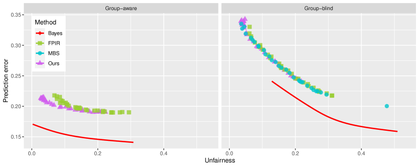
(a)

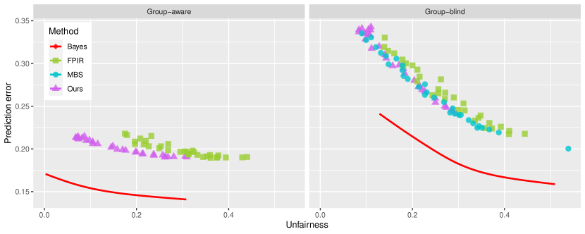
(b)

Figure 6: (a) The trade-off between prediction error and unfairness under (M3). The X-axis is the average unfairness measures $\bar{\mathcal{U}}_{\rm EOO}$ of the trained classifiers over 100 repetitions and the Y-axis is the average test prediction errors of these classifiers. The left and right panels correspond to the group-aware and group-blind scenarios, respectively. (b) As for (a) but the X-axis is the $95\%$ sample quantile ${\mathcal{U}}_{{\rm EOO},95}$ of the unfairness measures over 100 repetitions.

Figure 7: The curve of $|\lambda^{*G}_{\alpha}|$ on $\alpha$ under (M3). The red line is for the group-aware scenario and the cyan line is for the group-blind scenario.

Appendix C Derivation of Example 1

In the group-aware scenario, we have

$${\mathbb{P}}(Y_{f^{\rm aware}}(X,A)=1|Y=1,A=1)-{\mathbb{P}}(Y_{f^{\rm aware}}(X,A)=1|Y=1,A=2)$$

$$= {\mathbb{E}}(f^{\rm aware}(X,A)|Y=1,A=1)-{\mathbb{E}}(f^{\rm aware}(X,A)|Y=1,A=2)$$

$$= \frac{{\mathbb{E}}f^{\rm aware}(X,A){\mathbbm{1}}(Y=1,A=1)}{p_{1,1}}-\frac{{\mathbb{E}}f^{\rm aware}(X,A){\mathbbm{1}}(Y=1,A=2)}{p_{1,2}}$$

$$= \frac{{\mathbb{E}}{\mathbbm{1}}(A=1)\eta^{\rm aware}(X,A)f^{\rm aware}(X,A)}{p_{1,1}}-\frac{{\mathbb{E}}{\mathbbm{1}}(A=2)\eta^{\rm aware}(X,A)f^{\rm aware}(X,A)}{p_{1,2}}.$$

In the group-blind scenario, we have

$${\mathbb{P}}(Y_{f^{\rm blind}}(X,A)=1|Y=1,A=1)-{\mathbb{P}}(Y_{f^{\rm blind}}(X,A)=1|Y=1,A=2)$$

$$= {\mathbb{E}}(f^{\rm blind}(X,A)|Y=1,A=1)-{\mathbb{E}}(f^{\rm blind}(X,A)|Y=1,A=2)$$

$$= \frac{{\mathbb{E}}f^{\rm blind}(X,A){\mathbbm{1}}(Y=1,A=1)}{p_{1,1}}-\frac{{\mathbb{E}}f^{\rm blind}(X,A){\mathbbm{1}}(Y=1,A=2)}{p_{1,2}}$$

$$= \frac{{\mathbb{E}}\rho_{1|1}(X)\eta^{\rm blind}(X,A)f^{\rm blind}(X,A)}{p_{1,1}}-\frac{{\mathbb{E}}\rho_{2|1}(X)\eta^{\rm blind}(X,A)f^{\rm blind}(X,A)}{p_{1,2}}.$$

Appendix D Proofs of Propositions 1 and 2

Since Proposition 1 is a special case of Proposition 2, we only state the proof for the latter.

Proof of Proposition 2.

Since

$${\mathcal{R}}(f^{G})= {\mathbb{E}}{\mathbbm{1}}(Y=1,Y_{f^{G}}=0)+{\mathbbm{1}}(Y=0,Y_{f^{G}}=1)$$

$$= {\mathbb{E}}(1-f^{G}(X,A))\eta^{G}(X,A)+f^{G}(X,A)(1-\eta^{G}(X,A))$$

$$= p_{Y}+{\mathbb{E}}(1-2\eta^{G}(X,A))f^{G}(X,A),$$

we can rewrite $f^{*G}_{\alpha}$ as the solution of the problem

$$f^{*G}_{\alpha}\in \mathop{\rm arg\min}_{f^{G}\in[0,1]^{{\mathbb{R}}^{d}\times[K]}}{\mathbb{E}}(1-2\eta^{G}(X,A))f^{G}(X,A),\quad{\rm s.t.}\quad\|{\mathbb{E}}\Phi^{G}(X,A)f^{G}(X,A)\|\leq\alpha.$$ (25)

Considering the Lagrange function, Theorem 8.6.1 in Luenberger (1997) and Corollary 3.3 in Sion (1958) imply

$$\sup_{\lambda\in{\mathbb{R}}^{\tilde{K}}}{\mathbb{E}}\big{(}1-2\eta^{G}(X,A)+\lambda^{\top}\Phi^{G}(X,A)\big{)}f^{*G}_{\alpha}(X,A)-\alpha\|\lambda\|_{*}$$ (26)

$$= \sup_{\nu\geq 0}\sup_{\mu\in{\mathbb{R}}^{\tilde{K}},\|\mu\|_{*}\leq 1}{\mathbb{E}}\big{(}1-2\eta^{G}(X,A)+\nu\mu^{\top}\Phi^{G}(X,A)\big{)}f^{*G}_{\alpha}(X,A)-\nu\alpha$$

$$= \sup_{\nu\geq 0}{\mathbb{E}}(1-2\eta^{G}(X,A))f^{*G}_{\alpha}(X,A)+\nu(\|{\mathbb{E}}\Phi^{G}(X,A)f^{*G}_{\alpha}(X,A)\|-\alpha)$$

$$= \inf_{f^{G}\in[0,1]^{{\mathbb{R}}^{d}\times[K]}}\sup_{\nu\geq 0}{\mathbb{E}}(1-2\eta^{G}(X,A))f^{G}(X,A)+\nu(\|{\mathbb{E}}\Phi^{G}(X,A)f^{G}(X,A)\|-\alpha)$$

$$\overset{\text{\cite[cite]{\@@bibref{Authors Phrase1YearPhrase2}{luenberger1997optimization}{\@@citephrase{(}}{\@@citephrase{)}}}}}{=} \sup_{\nu\geq 0}\inf_{f^{G}\in[0,1]^{{\mathbb{R}}^{d}\times[K]}}{\mathbb{E}}(1-2\eta^{G}(X,A))f^{G}(X,A)+\nu(\|{\mathbb{E}}\Phi^{G}(X,A)f^{G}(X,A)\|-\alpha)$$

$$= \sup_{\nu\geq 0}\inf_{f^{G}\in[0,1]^{{\mathbb{R}}^{d}\times[K]}}\sup_{\mu\in{\mathbb{R}}^{\tilde{K}},\|\mu\|_{*}\leq 1}{\mathbb{E}}\big{(}1-2\eta^{G}(X,A)+\nu\mu^{\top}\Phi^{G}(X,A)\big{)}f^{G}(X,A)-\nu\alpha$$

$$\overset{\text{\cite[cite]{\@@bibref{Authors Phrase1YearPhrase2}{sion1958general}{\@@citephrase{(}}{\@@citephrase{)}}}}}{=} \sup_{\nu\geq 0}\sup_{\mu\in{\mathbb{R}}^{\tilde{K}},\|\mu\|_{*}\leq 1}\inf_{f^{G}\in[0,1]^{{\mathbb{R}}^{d}\times[K]}}{\mathbb{E}}\big{(}1-2\eta^{G}(X,A)+\nu\mu^{\top}\Phi^{G}(X,A)\big{)}f^{G}(X,A)-\nu\alpha$$

$$= \sup_{\lambda\in{\mathbb{R}}^{\tilde{K}}}\inf_{f^{G}\in[0,1]^{{\mathbb{R}}^{d}\times[K]}}{\mathbb{E}}\big{(}1-2\eta^{G}(X,A)+\lambda^{\top}\Phi^{G}(X,A)\big{)}f^{G}(X,A)-\alpha\|\lambda\|_{*}$$

$$= -\inf_{\lambda\in{\mathbb{R}}^{\tilde{K}}}\big{\{}{\mathbb{E}}\big{(}2\eta^{G}(X,A)-1-\lambda^{\top}\Phi^{G}(X,A)\big{)}_{+}+\alpha\|\lambda\|_{*}\big{\}}.$$

Denote

$$\mu^{*}_{\alpha}\in\mathop{\rm arg\max}_{\lambda\in{\mathbb{R}}^{\tilde{K}}}{\mathbb{E}}\big{(}1-2\eta^{G}(X,A)+\lambda^{\top}\Phi^{G}(X,A)\big{)}f^{*G}_{\alpha}(X,A)-\alpha\|\lambda\|_{*},$$

$$\lambda^{*}_{\alpha}\in\mathop{\rm arg\min}_{\lambda\in{\mathbb{R}}^{\tilde{K}}}{\mathbb{E}}\big{(}2\eta^{G}(X,A)-1-\lambda^{\top}\Phi^{G}(X,A)\big{)}_{+}+\alpha\|\lambda\|_{*},$$

$$h^{*G}_{\alpha}(X,A)= {\mathbbm{1}}\big{(}2\eta^{G}(X,A)-1-\lambda^{*\top}_{\alpha}\Phi^{G}(X,A)>0\big{)}$$

$$+\tilde{b}^{G}(X,A){\mathbbm{1}}\big{(}2\eta^{G}(X,A)-1-\lambda^{*\top}_{\alpha}\Phi^{G}(X,A)=0\big{)},$$

for some $\tilde{b}^{G}\in[0,1]^{{\mathbb{R}}^{d}\times[K]}$ and

$$g^{G}(f^{G},\lambda)={\mathbb{E}}\big{(}1-2\eta^{G}(X,A)+\lambda^{\top}\Phi^{G}(X,A)\big{)}f^{G}(X,A)-\alpha\|\lambda\|_{*},$$

we know

$$g^{G}(h_{\alpha}^{*G},\lambda^{*}_{\alpha})\leq g^{G}(f^{*G}_{\alpha},\lambda^{*}_{\alpha})\leq g^{G}(f^{*G}_{\alpha},\mu^{*}_{\alpha}).$$

Together with Equation (26) gives

$$g^{G}(h^{*G}_{\alpha},\lambda^{*}_{\alpha})=g^{G}(f^{*G}_{\alpha},\lambda^{*}_{\alpha})=g^{G}(f^{*G}_{\alpha},\mu^{*}_{\alpha}).$$ (27)

The first equality in (27) implies that $f^{*G}_{\alpha}$ must have the following form $P_{X,A}$-almost surely,

$$f^{*G}_{\alpha}(X,A)= {\mathbbm{1}}\big{(}2\eta^{G}(X,A)-1-\lambda^{*\top}_{\alpha}\Phi^{G}(X,A)>0\big{)}$$

$$+b^{G}(X,A){\mathbbm{1}}\big{(}2\eta^{G}(X,A)-1-\lambda^{*\top}_{\alpha}\Phi^{G}(X,A)=0\big{)}.$$

The second equality in (27) implies

$$\lambda^{*}_{\alpha}\in\mathop{\rm arg\max}_{\lambda\in{\mathbb{R}}^{\tilde{K}}}{\mathbb{E}}\lambda^{\top}\Phi^{G}(X,A)f^{*G}_{\alpha}(X,A)-\alpha\|\lambda\|_{*}.$$

We denote $\nu^{*}=\|\lambda^{*}_{\alpha}\|$, if $\nu^{*}=0$, then it holds trivially that

$$\lambda^{*\top}_{\alpha}{\mathbb{E}}\Phi^{G}(X,A)f^{*G}_{\alpha}(X,A)=\|\lambda^{*}_{\alpha}\|_{*}\|{\mathbb{E}}\Phi^{G}(X,A)f^{*G}_{\alpha}(X,A)\|=\alpha\|\lambda^{*}_{\alpha}\|_{*}.$$

If $\nu^{*}\neq 0$, we let $\mu^{*}=\frac{\lambda^{*}_{\alpha}}{\nu^{*}}$, then it is straightforward that

$$(\nu^{*},\mu^{*})\in\mathop{\rm arg\max}_{(\nu,\mu):\nu\geq 0,\mu\in{\mathbb{R}}^{\tilde{K}},\|\mu\|_{*}\leq 1}Q(\nu,\mu),\quad Q(\nu,\mu)={\mathbb{E}}\nu\mu^{\top}\Phi^{G}(X,A)f^{*G}(X,A)-\alpha\nu.$$

Since $\mu^{*}\in\mathop{\rm arg\max}_{\mu\in{\mathbb{R}}^{\tilde{K}},\|\mu\|_{*}\leq 1}Q(\nu^{*},\mu)$, we know

$$\mu^{*\top}_{\alpha}{\mathbb{E}}\Phi^{G}(X,A)f^{*G}_{\alpha}(X,A)=\|{\mathbb{E}}\Phi^{G}(X,A)f^{*G}_{\alpha}(X,A)\|.$$

Similarly, since $\nu^{*}\in\mathop{\rm arg\max}_{\nu\geq 0}Q(\nu,\mu^{*})$ and $\|{\mathbb{E}}\Phi^{G}(X,A)f^{*G}_{\alpha}(X,A)\|\leq\alpha$, $\nu^{*}>0$ implies

$$\|{\mathbb{E}}\Phi^{G}(X,A)f^{*G}_{\alpha}(X,A)\|=\alpha.$$

In conclusion, we have

$$\lambda^{*\top}_{\alpha}{\mathbb{E}}\Phi^{G}(X,A)f^{*G}_{\alpha}(X,A)=\|\lambda^{*}_{\alpha}\|_{*}\|{\mathbb{E}}\Phi^{G}(X,A)f^{*G}_{\alpha}(X,A)\|=\alpha\|\lambda^{*}_{\alpha}\|_{*}.$$

Moreover, since the first three lines in Equation (26) holds for any classifier $f^{G}$, we know any minimizer of

$$\mathop{\rm arg\min}_{f^{G}\in[0,1]^{{\mathbb{R}}^{d}\times[K]}}\sup_{\lambda\in{\mathbb{R}}^{\tilde{K}}}g^{G}(f^{G},\lambda)$$

is a Bayes optimal classifier. For any function $b^{G}\in[0,1]^{{\mathbb{R}}^{d}\times[K]}$ such that

$$\|{\mathbb{E}}\Phi^{G}(X,A)h^{G}(X,A)\|\leq\alpha,\quad\lambda^{*\top}_{\alpha}{\mathbb{E}}\Phi^{G}(X,A)h^{G}(X,A)=\|\lambda^{*}_{\alpha}\|_{*}\|{\mathbb{E}}\Phi^{G}(X,A)h^{G}(X,A)\|=\alpha\|\lambda^{*}_{\alpha}\|_{*},$$

with

$$h^{G}={\mathbbm{1}}\big{(}2\eta^{G}-1-\lambda^{*\top}_{\alpha}\Phi^{G}>0\big{)}+b^{G}{\mathbbm{1}}\big{(}2\eta^{G}-1-\lambda^{*\top}_{\alpha}\Phi^{G}=0\big{)},$$

we have

$$\sup_{\lambda\in{\mathbb{R}}^{\tilde{K}}}g^{G}(h^{G},\lambda)= {\mathbb{E}}\big{(}1-2\eta^{G}(X,A)\big{)}h^{G}(X,A)+\sup_{\lambda\in{\mathbb{R}}^{\tilde{K}}}{\mathbb{E}}\lambda^{\top}\Phi^{G}(X,A)h^{G}(X,A)-\alpha\|\lambda\|_{*}$$

$$= {\mathbb{E}}\big{(}1-2\eta^{G}(X,A)\big{)}h^{G}(X,A)$$

$$= {\mathbb{E}}\big{(}1-2\eta^{G}(X,A)\big{)}h^{G}(X,A)+\lambda^{*\top}_{\alpha}{\mathbb{E}}\Phi^{G}(X,A)h^{G}(X,A)-\alpha\|\lambda^{*}_{\alpha}\|_{*}$$

$$= g^{G}(h^{G},\lambda^{*}_{\alpha})$$

$$= g^{G}(f^{*G}_{\alpha},\lambda^{*}_{\alpha})$$

$$= \inf_{f^{G}\in[0,1]^{{\mathbb{R}}^{d}\times[K]}}\sup_{\lambda\in{\mathbb{R}}^{\tilde{K}}}g^{G}(f^{G},\lambda),$$

where the last equality comes from the fact that $(f^{*G}_{\alpha},\lambda^{*})$ is a saddle point due to Equation (27). Therefore $h^{G}$ is a Bayes optimal classifier. ∎

Appendix E Proof of Lemmas 1 and 2

Proof of Lemma 1.

Denote $s_{\lambda}={\rm sgn}(\lambda^{*}_{\alpha})$ with ${\rm sgn}(0)\in[-1,1]$, we separate the proof into two cases depending on whether $\lambda^{*}_{\alpha}=0$.

1. If $\lambda^{*}_{\alpha}=0$, we have $|{\mathbb{E}}\phi^{G}(X,A){\mathbbm{1}}\big{(}2\eta^{G}(X,A)>1\big{)}|\leq\alpha$. Then $|\lambda^{*}_{\alpha}|=0$ is the smallest non-negative real number $\lambda_{+}$ such that

   $$s{\mathbb{E}}\phi^{G}(X,A){\mathbbm{1}}\big{(}2\eta^{G}(X,A)-1>s\lambda_{+}\phi^{G}(X,A)\big{)}\leq\alpha.$$

2. If $\lambda^{*}_{\alpha}\neq 0$, we know

   $$s_{\lambda}{\mathbb{E}}\phi^{G}(X,A){\mathbbm{1}}\big{(}2\eta^{G}(X,A)-1>s_{\lambda}|\lambda^{*}_{\alpha}|\phi^{G}(X,A)\big{)}=\alpha.$$

   Due to the non-increasing property of

   $$\lambda_{+}\rightarrow s_{\lambda}{\mathbb{E}}\phi^{G}(X,A){\mathbbm{1}}\big{(}2\eta^{G}(X,A)-1>s_{\lambda}\lambda_{+}\phi^{G}(X,A)\big{)},$$

   we get

   $$s_{\lambda}{\mathbb{E}}\phi^{G}(X,A){\mathbbm{1}}\big{(}2\eta^{G}(X,A)>1\big{)}\geq s_{\lambda}{\mathbb{E}}\phi^{G}(X,A){\mathbbm{1}}\big{(}2\eta^{G}(X,A)-1>s_{\lambda}|\lambda^{*}_{\alpha}|\phi^{G}(X,A)\big{)}\geq\alpha,$$

   which implies $s=s_{\lambda}$.

   In the following, we prove that $|\lambda^{*}_{\alpha}|$ is the smallest non-negative real number $\lambda_{+}$ such that

   $$s{\mathbb{E}}\phi^{G}(X,A){\mathbbm{1}}\big{(}2\eta^{G}(X,A)-1>s\lambda_{+}\phi^{G}(X,A)\big{)}\leq\alpha.$$

   To this end, suppose there exists $0\leq\lambda_{+}<|\lambda^{*}_{\alpha}|$ such that the above inequality is satisfied. It follows from the monotonicity that

   $$s{\mathbb{E}}\phi^{G}(X,A){\mathbbm{1}}\big{(}2\eta^{G}(X,A)-1>s\lambda_{+}\phi^{G}(X,A)\big{)}=\alpha.$$

   Denote $\Delta=|\lambda^{*}_{\alpha}|-\lambda_{+}$ and $g^{*G}_{\alpha}=2\eta^{G}-1-\lambda^{*}_{\alpha}\phi^{G}$, we have

   $$0= s{\mathbb{E}}\phi^{G}(X,A){\mathbbm{1}}\big{(}2\eta^{G}(X,A)-1>s|\lambda^{*}_{\alpha}|\phi^{G}(X,A)\big{)}$$

   $$-s{\mathbb{E}}\phi^{G}(X,A){\mathbbm{1}}\big{(}2\eta^{G}(X,A)-1>s\lambda_{+}\phi^{G}(X,A)\big{)}$$

   $$= s{\mathbb{E}}\phi^{G}(X,A){\mathbbm{1}}\big{(}-s\Delta\phi^{G}(X,A)\geq g^{*G}_{\alpha}(X,A)>0\big{)}$$

   $$-s{\mathbb{E}}\phi^{G}(X,A){\mathbbm{1}}\big{(}-s\Delta\phi^{G}(X,A)<g^{*G}_{\alpha}(X,A)\leq 0\big{)}$$

   $$= -{\mathbb{E}}|\phi^{G}(X,A)|{\mathbbm{1}}\big{(}\Delta|\phi^{G}(X,A)|\geq g^{*G}_{\alpha}(X,A)>0,s\phi^{G}(X,A)<0\big{)}$$

   $$-{\mathbb{E}}|\phi^{G}(X,A)|{\mathbbm{1}}\big{(}-\Delta|\phi^{G}(X,A)|<g^{*G}_{\alpha}(X,A)\leq 0,s\phi^{G}(X,A)>0\big{)},$$

   which implies

   $${\mathbb{P}}\big{(}\Delta|\phi^{G}(X,A)|\geq g^{*G}_{\alpha}(X,A)>0,s\phi^{G}(X,A)<0\big{)}=0,$$

   $${\mathbb{P}}\big{(}-\Delta|\phi^{G}(X,A)|<g^{*G}_{\alpha}(X,A)\leq 0,s\phi^{G}(X,A)>0\big{)}=0.$$

   Then we check Problem (5) at $s\lambda_{+}$.

   $$\bigg{(}{\mathbb{E}}\big{(}2\eta^{G}(X,A)-1-\lambda^{*}_{\alpha}\phi^{G}(X,A)\big{)}_{+}+\alpha|\lambda^{*}|\bigg{)}-\bigg{(}{\mathbb{E}}\big{(}2\eta^{G}(X,A)-1-s\lambda_{+}\phi^{G}(X,A)\big{)}_{+}+\alpha\lambda_{+}\bigg{)}$$

   $$= {\mathbb{E}}\big{(}2\eta^{G}(X,A)-1\big{)}{\mathbbm{1}}\big{(}2\eta^{G}(X,A)-1>\lambda^{*}_{\alpha}\phi^{G}(X,A)\big{)}$$

   $$-{\mathbb{E}}\big{(}2\eta^{G}(X,A)-1\big{)}{\mathbbm{1}}\big{(}2\eta^{G}(X,A)-1>s\lambda_{+}\phi^{G}(X,A)\big{)}$$

   $$= {\mathbb{E}}\big{(}2\eta^{G}(X,A)-1\big{)}{\mathbbm{1}}\big{(}-s\Delta\phi^{G}(X,A)\geq g^{*G}_{\alpha}(X,A)>0\big{)}$$

   $$-{\mathbb{E}}\big{(}2\eta^{G}(X,A)-1\big{)}{\mathbbm{1}}\big{(}-s\Delta\phi^{G}(X,A)<g^{*G}_{\alpha}(X,A)\leq 0\big{)}$$

   $$= {\mathbb{E}}\big{(}2\eta^{G}(X,A)-1\big{)}{\mathbbm{1}}(\Delta|\phi^{G}(X,A)|\geq g^{*G}_{\alpha}(X,A)>0,s\phi^{G}(X,A)<0\big{)}$$

   $$-{\mathbb{E}}\big{(}2\eta^{G}(X,A)-1\big{)}{\mathbbm{1}}(\Delta|\phi^{G}(X,A)|<g^{*G}_{\alpha}(X,A)\leq 0,s\phi^{G}(X,A)>0\big{)}$$

   $$= 0.$$

   So $s\lambda_{+}$ is also a minimizer of Problem (5) with $\lambda_{+}<|\lambda^{*}_{\alpha}|$ which contradicts the definition of $\lambda^{*}_{\alpha}$. Then we conclude the result that $|\lambda^{*}_{\alpha}|$ is the smallest non-negative real number $\lambda_{+}$ such that

   $$s{\mathbb{E}}\phi^{G}(X,A){\mathbbm{1}}\big{(}2\eta^{G}(X,A)-1>s\lambda_{+}\phi^{G}(X,A)\big{)}\leq\alpha.$$

Combining pieces proves the lemma. ∎

Proof of Lemma 2.

At first we show the existence of $\tilde{\lambda}_{+}$. Since

$$\tilde{s}^{G}{\mathbb{E}}\phi^{G}(X,A){\mathbbm{1}}\big{(}2\hat{\eta}^{G}(X,A)-1>\tilde{s}^{G}\lambda_{+}\phi^{G}(X,A)\big{)}$$

$$= {\mathbb{E}}|\phi^{G}(X,A)|{\mathbbm{1}}\big{(}2\hat{\eta}^{G}(X,A)-1>\lambda_{+}|\phi^{G}(X,A)|,\tilde{s}^{G}\phi^{G}(X,A)>0\big{)}$$

$$-{\mathbb{E}}|\phi^{G}(X,A)|{\mathbbm{1}}\big{(}2\hat{\eta}^{G}(X,A)-1>-\lambda_{+}|\phi^{G}(X,A)|,\tilde{s}^{G}\phi^{G}(X,A)<0\big{)},$$

which is non-positive when $\lambda_{+}$ increases to infinity. Therefore $\tilde{\lambda}_{+}$ is always well defined.

Then we verify the unfairness control in two cases.

Case (1): If $\tilde{\lambda}_{+}=0$, it follows from the definition of $\tilde{s}^{G}$ and $\tilde{\lambda}_{+}$ that

$$\tilde{s}^{G}{\mathbb{E}}\phi^{G}(X,A){\mathbbm{1}}\big{(}2\hat{\eta}^{G}(X,A)>1\big{)}\in[0,\alpha],$$

which implies

$${\mathcal{U}}({\mathbbm{1}}(2\hat{\eta}^{G}>1))\leq\alpha.$$

Case (2): If $\tilde{\lambda}_{+}>0$, since

$$\sup_{\lambda\in{\mathbb{R}}}{\mathbb{P}}(2\hat{\eta}^{G}(X,A)-1=\lambda\phi^{G}(X,A))=0,$$

we know

$$\tilde{s}^{G}{\mathbb{E}}\phi^{G}(X,A){\mathbbm{1}}\big{(}2\hat{\eta}^{G}(X,A)-1>\tilde{s}^{G}\lambda_{+}\phi^{G}(X,A)\big{)}=\alpha.$$

Therefore ${\mathcal{U}}({\mathbbm{1}}(2\hat{\eta}^{G}-1>\tilde{s}^{G}\tilde{\lambda}_{+}\phi^{G}))=\alpha$. ∎

Appendix F Proofs of Lemmas 3 and 6

Lemmas 3 and 6 follow directly from the following Lemma 7, which can be obtained from Theorem 12.1 and Theorem 13.7 in Boucheron et al. (2013).

Lemma 7 (Empirical Process).

Suppose $Z_{1},\ldots,Z_{n}\overset{\rm i.i.d.}{\sim}Z\in\mathcal{Z}$ and $\mathcal{C}$ is a class of subsets of $\mathcal{Z}$ with finite VC dimension $v$, then with probability at least $1-\delta$, we have

$$\sup_{C\in\mathcal{C}}\left|\frac{1}{n}\sum_{i=1}^{n}{\mathbbm{1}}(Z_{i}\in C)-{\mathbb{P}}(Z\in\mathcal{C})\right|\leq 72\sqrt{\frac{v\log 4e^{2}}{n}}+\sqrt{\frac{1}{2n}\log\frac{2}{\delta}}.$$

Appendix G Modification to $\hat{\eta}^{G},\hat{\phi}^{G}$ for fulfilling Assumption 1

Without loss of generality, we assume ${\mathbb{P}}_{X,A}(\hat{\phi}^{G}(X,A)=0)=0$, otherwise, we can replace $\hat{\phi}^{G}$ by $\tilde{\phi}^{G}=\hat{\phi}^{G}+\epsilon_{\phi}{\mathbbm{1}}(\hat{\phi}^{G}=0)$. Then ${\mathbb{P}}_{X,A}(\tilde{\phi}^{G}(X,A)=0)=0$ and $\|\tilde{\phi}^{G}-\phi^{G}\|_{\infty}\leq 2\epsilon_{\phi}$. Similarly, we assume ${\mathbb{P}}_{X,A}(2\hat{\eta}^{G}(X,A)=1)=0$, otherwise, we replace $\hat{\eta}^{G}$ by $\tilde{\eta}^{G}=\hat{\eta}^{G}+\epsilon_{\eta}{\mathbbm{1}}(2\hat{\eta}^{G}=1)$, then ${\mathbb{P}}_{X,A}(2\tilde{\eta}^{G}(X,A)=1)=0$ and $\|\tilde{\eta}^{G}-\eta^{G}\|_{\infty}\leq 2\epsilon_{\eta}$.

If $X|A$ is continuous, we know ${\mathbb{P}}_{X,A}\big{(}2\hat{\eta}^{G}(X,A)-1=\lambda\hat{\phi}^{G}(X,A)\big{)}>0$ if and only if ${\rm Leb}(S_{\lambda})>0$ with $S_{\lambda}=\big{\{}x:2\hat{\eta}^{G}(x,a)-1=\lambda\hat{\phi}^{G}(x,a),a\in[2]\big{\}},\lambda\neq 0$. Since the CDF of $\frac{2\hat{\eta}^{G}(X,A)-1}{\hat{\phi}^{G}(X,A)}$ conditioned on $\hat{\eta}^{G},\hat{\phi}^{G}$ has at most countably many discontinuous points, there are only countably many $\lambda$’s such that ${\rm Leb}(S_{\lambda})>0$. For any such $\lambda\in{\mathbb{R}}$, on the set $S_{\lambda}$, we replace $\hat{\eta}^{G}(x,a)$ by $\tilde{\eta}^{G}(x,a)=\hat{\eta}^{G}(x,a)+(\frac{1}{2}-\hat{\eta}^{G}(x,a))\epsilon_{\eta}|\sin(x_{1})|$ with $x_{1}$ to be the first coordinate of $x$. Then it is straightforward to verify that ${\rm Leb}(S_{\lambda}\cap\tilde{S}_{\tilde{\lambda}})={\rm Leb}\{\epsilon_{\eta}|\sin(x_{1})|=1-\frac{\tilde{\lambda}}{\lambda}\}=0$ for all $\tilde{\lambda}\in{\mathbb{R}}$ where $\tilde{S}_{\lambda}=\big{\{}x:2\tilde{\eta}^{G}(x,a)-1=\lambda\hat{\phi}^{G}(x,a),a\in[2]\big{\}}$. Moreover $\sup_{x\in S_{\lambda},a\in[2]}|\tilde{\eta}^{G}(x,a)-\eta^{G}(x,a)|\leq\frac{3}{2}\epsilon_{\eta}$. Therefore Assumption 1 is met after the modification.

Appendix H Proof of Theorem 1

Proof of Theorem 1.

Throughout the proof, the expectations are taken with respect to a new test sample $(X,A,Y)$ conditioned on the dataset ${\mathcal{D}}$.

Existence of $\hat{\lambda}^{G}$:

Denote the event $E$ as

$$E=\bigg{\{}\sup_{\lambda\in{\mathbb{R}}}\bigg{|}\sum_{j\in[m]}\kappa_{j}(\hat{\mathbb{E}}_{j}-{\mathbb{E}}_{j}){\mathbbm{1}}\big{(}2\hat{\eta}^{G}(X,A)-1>\lambda\hat{\phi}^{G}(X,A)\big{)}\bigg{|}\leq\epsilon_{\alpha}\bigg{\}},$$

Lemma 3 implies ${\mathbb{P}}(E^{c})\leq\delta_{\rm post}$. Under event $E$, we have

$$\hat{s}^{G}\sum_{j\in[m]}\kappa_{j}\hat{\mathbb{E}}_{j}{\mathbbm{1}}\big{(}2\hat{\eta}^{G}(X,A)-1>\hat{s}^{G}\lambda_{+}\hat{\phi}^{G}(X,A)\big{)}$$

$$\leq \hat{s}^{G}\sum_{j\in[m]}\kappa_{j}{\mathbb{E}}_{j}{\mathbbm{1}}\big{(}2\hat{\eta}^{G}(X,A)-1>\hat{s}^{G}\lambda_{+}\hat{\phi}^{G}(X,A)\big{)}+\epsilon_{\alpha}$$

$$= \hat{s}^{G}{\mathbb{E}}\phi^{G}(X,A){\mathbbm{1}}\big{(}2\hat{\eta}^{G}(X,A)-1>\hat{s}^{G}\lambda_{+}\hat{\phi}^{G}(X,A)\big{)}+\epsilon_{\alpha}$$

$$\leq \hat{s}^{G}{\mathbb{E}}\phi^{G}(X,A){\mathbbm{1}}\big{(}2\hat{\eta}^{G}(X,A)-1>\hat{s}^{G}\lambda_{+}\hat{\phi}^{G}(X,A),\phi^{G}(X,A)\hat{\phi}^{G}(X,A)>0\big{)}$$

$$+{\mathbb{E}}|\phi^{G}(X,A)|{\mathbbm{1}}\big{(}\phi^{G}(X,A)\hat{\phi}^{G}(X,A)\leq 0\big{)}+\epsilon_{\alpha}.$$

$$= \underbrace{{\mathbb{E}}|\phi^{G}(X,A)|{\mathbbm{1}}\big{(}2\hat{\eta}^{G}(X,A)-1>\lambda_{+}|\hat{\phi}^{G}(X,A)|,\phi^{G}(X,A)\hat{\phi}^{G}(X,A)>0,\hat{s}^{G}\phi^{G}(X,A)>0\big{)}}_{T_{1}}$$

$$-\underbrace{{\mathbb{E}}|\phi^{G}(X,A)|{\mathbbm{1}}\big{(}2\hat{\eta}^{G}(X,A)-1>-\lambda_{+}|\hat{\phi}^{G}(X,A)|,\phi^{G}(X,A)\hat{\phi}^{G}(X,A)>0,\hat{s}^{G}\phi^{G}(X,A)<0\big{)}}_{T_{2}}$$

$$+\tilde{\epsilon}_{\phi}^{G}+\epsilon_{\alpha}$$

It is not hard to see that $T_{1}-T_{2}$ are non-increasing in $\lambda_{+}$ and $\lim_{\lambda_{+}\rightarrow+\infty}T_{1}-T_{2}\leq 0$. Since $\alpha\geq 2\epsilon_{\alpha}+\tilde{\epsilon}_{\phi}^{G}$, for $\lambda_{+}$ large enough, we have

$$\hat{s}^{G}\sum_{j\in[m]}\kappa_{j}\hat{\mathbb{E}}_{j}{\mathbbm{1}}\big{(}2\hat{\eta}^{G}(X,A)-1>\hat{s}^{G}\lambda_{+}\hat{\phi}^{G}(X,A)\big{)}\leq\tilde{\epsilon}_{\phi}^{G}+\epsilon_{\alpha}\leq\alpha-\epsilon_{\alpha},$$

which implies $\hat{\lambda}_{+}^{G}$ is well defined.

Fairness constraint:

We prove this part by considering two cases separately.

Case (1): If

$$\hat{s}^{G}\sum_{j\in[m]}\kappa_{j}\hat{\mathbb{E}}_{j}{\mathbbm{1}}\big{(}2\hat{\eta}^{G}(X,A)-1>\hat{\lambda}^{G}\hat{\phi}^{G}(X,A)\big{)}\leq\alpha-\epsilon_{\alpha},$$

we know that under event $E$,

$$\hat{s}^{G}{\mathbb{E}}\phi^{G}(X,A){\mathbbm{1}}\big{(}2\hat{\eta}^{G}(X,A)-1>\hat{\lambda}^{G}\hat{\phi}^{G}(X,A)\big{)}$$

$$\leq \hat{s}^{G}\sum_{j\in[m]}\kappa_{j}\hat{\mathbb{E}}_{j}{\mathbbm{1}}\big{(}2\hat{\eta}^{G}(X,A)-1>\hat{\lambda}^{G}\hat{\phi}^{G}(X,A)\big{)}+\epsilon_{\alpha}$$

$$\leq \alpha.$$

If $\hat{\lambda}^{G}=0$, we get

$$-\hat{s}^{G}{\mathbb{E}}\phi^{G}(X,A){\mathbbm{1}}\big{(}2\hat{\eta}^{G}(X,A)>1\big{)}$$

$$\leq -\hat{s}^{G}\sum_{j\in[m]}\kappa_{j}\hat{\mathbb{E}}_{j}{\mathbbm{1}}\big{(}2\hat{\eta}^{G}(X,A)>1\big{)}+\epsilon_{\alpha}$$

$$\leq \epsilon_{\alpha}$$

$$\leq \alpha.$$

If $\hat{\lambda}^{G}_{+}>0$, for any $0<\Delta\leq\hat{\lambda}_{+}^{G}$, it follows from the definition of $\hat{\lambda}_{+}^{G}$ that

$$-\hat{s}^{G}{\mathbb{E}}\phi^{G}(X,A){\mathbbm{1}}\big{(}2\hat{\eta}^{G}(X,A)-1>\hat{s}^{G}(\hat{\lambda}_{+}^{G}-\Delta)\hat{\phi}^{G}(X,A)\big{)}$$ (28)

$$\leq -\hat{s}^{G}\sum_{j\in[m]}\kappa_{j}\hat{\mathbb{E}}_{j}{\mathbbm{1}}\big{(}2\hat{\eta}^{G}(X,A)-1>\hat{s}^{G}(\hat{\lambda}_{+}^{G}-\Delta)\hat{\phi}^{G}(X,A)\big{)}+\epsilon_{\alpha}$$

$$\leq -\alpha+2\epsilon_{\alpha}$$

$$\leq \alpha.$$

Setting $\Delta\rightarrow 0+$, since $\phi^{G}$ is bounded, then the continuity in Assumption 1 implies

$$-\hat{s}^{G}{\mathbb{E}}\phi^{G}(X,A){\mathbbm{1}}\big{(}2\hat{\eta}^{G}(X,A)-1>\hat{\lambda}^{G}\hat{\phi}^{G}(X,A)\big{)}\leq\alpha.$$

Therefore, under the event $E$, we have

$${\mathcal{U}}(\hat{f}^{G}_{\alpha})=|{\mathbb{E}}\phi^{G}(X,A){\mathbbm{1}}\big{(}2\hat{\eta}^{G}(X,A)-1>\hat{\lambda}^{G}\hat{\phi}^{G}(X,A)\big{)}|\leq\alpha.$$

Case (2): If the empirical unfairness measure in Step 2 of Algorithm 1 jumps at $\hat{\lambda}^{G}_{+}$ such that

$$\hat{s}^{G}\sum_{j\in[m]}\kappa_{j}\hat{\mathbb{E}}_{j}{\mathbbm{1}}\big{(}2\hat{\eta}^{G}(X,A)-1>\hat{\lambda}^{G}\hat{\phi}^{G}(X,A)\big{)}>\alpha-\epsilon_{\alpha},$$

then there exists a sequence $\{\lambda_{+t}:i\in{\mathbb{N}}_{+}\}$ such that $\lambda_{+t}\searrow\hat{\lambda}^{G}_{+}$ and

$$\hat{s}^{G}\sum_{j\in[m]}\kappa_{j}\hat{\mathbb{E}}_{j}{\mathbbm{1}}\big{(}2\hat{\eta}^{G}(X,A)-1>\hat{s}^{G}\lambda_{+t}\hat{\phi}^{G}(X,A)\big{)}\leq\alpha-\epsilon_{\alpha},\quad\forall t\in{\mathbb{N}}_{+}.$$

Then

$$\hat{s}^{G}{\mathbb{E}}\phi^{G}(X,A){\mathbbm{1}}\big{(}2\hat{\eta}^{G}(X,A)-1>\hat{s}^{G}\lambda_{+t}\hat{\phi}^{G}(X,A)\big{)}$$

$$\leq \hat{s}^{G}\sum_{j\in[m]}\kappa_{j}\hat{\mathbb{E}}_{j}{\mathbbm{1}}\big{(}2\hat{\eta}^{G}(X,A)-1>\hat{s}^{G}\lambda_{+t}\hat{\phi}^{G}(X,A)\big{)}+\epsilon_{\alpha}$$

$$\leq \alpha.$$

Setting $t\rightarrow\infty$, since $\phi^{G}$ is bounded, then the continuity in Assumption 1 implies that

$$\hat{s}^{G}{\mathbb{E}}\phi^{G}(X,A){\mathbbm{1}}\big{(}2\hat{\eta}^{G}(X,A)-1>\hat{\lambda}^{G}\hat{\phi}^{G}(X,A)\big{)}\leq\alpha.$$

Using the same proof with Case (1), we can also show that under the event $E$,

$${\mathcal{U}}(\hat{f}^{G}_{\alpha})\leq\alpha.$$

∎

Appendix I Derivations in Remark 3

Assumption 3 supposes the unfairness difference $D$ satisfies that for any $\tilde{z}\in{\mathbb{R}}$,

$$D(4\tilde{z})\leq c_{2}D(\tilde{z}).$$

It is not hard to see that

$$\forall|z^{\prime}|\geq|\tilde{z}|>0,~{}\tilde{z}z^{\prime}>0,~{}1\geq\frac{D(\tilde{z})}{D(z^{\prime})}\geq\bigg{(}\frac{\tilde{z}}{z^{\prime}}\bigg{)}^{\log_{4}c_{2}}$$

$$\Longrightarrow \forall\tilde{z}\in{\mathbb{R}},~{}D(4\tilde{z})\leq c_{2}D(\tilde{z})$$

$$\Longrightarrow \forall|z^{\prime}|\geq|\tilde{z}|>0,~{}\tilde{z}z^{\prime}>0,~{}1\geq\frac{D(\tilde{z})}{D(z^{\prime})}\geq\bigg{(}\frac{\tilde{z}}{4z^{\prime}}\bigg{)}^{\log_{4}c_{2}}.$$

If we fix $z^{\prime}$ such that $|z^{\prime}|$ is a large constant, under Assumption 3, for any $\tilde{z}\in{\mathbb{R}}$ with $\tilde{z}z^{\prime}\geq 0$, $|\tilde{z}|\leq|z^{\prime}|$, we see

$$D(\tilde{z})\gtrsim|\tilde{z}|^{\log_{4}c_{2}}.$$

Appendix J Proof of Theorem 2

Proof of Theorem 2.

Throughout the proof, the expectations are taken with respect to a new test sample $(X,A,Y)$ conditioned on the dataset ${\mathcal{D}}$.

The excess risk of $\hat{f}^{G}$ can be expressed as

$${\mathcal{R}}(\hat{f}^{G}_{\alpha})-{\mathcal{R}}(f^{*G}_{\alpha})$$

$$= {\mathbb{E}}(2\eta^{G}(X,A)-1)(f^{*G}_{\alpha}(X,A)-\hat{f}^{G}_{\alpha}(X,A))$$

$$= \underbrace{{\mathbb{E}}\left|2\eta^{G}(X,A)-1-\lambda^{*G}_{\alpha}\phi^{G}(X,A)\right|\left|f^{*G}_{\alpha}(X,A)-\hat{f}^{G}_{\alpha}(X,A)\right|}_{T_{1}}+\underbrace{{\mathbb{E}}\lambda^{*G}_{\alpha}\phi^{G}(X,A)(f^{*G}_{\alpha}(X,A)-\hat{f}^{G}_{\alpha}(X,A))}_{T_{2}}.$$

We denote $U(0)={\mathcal{U}}({\mathbbm{1}}(2\eta^{G}>1))$ and

$$E=\bigg{\{}\sup_{\lambda\in{\mathbb{R}}}\bigg{|}\sum_{j\in[m]}\kappa_{j}(\hat{\mathbb{E}}_{j}-{\mathbb{E}}_{j}){\mathbbm{1}}\big{(}2\hat{\eta}^{G}(X,A)-1>\lambda\hat{\phi}^{G}(X,A)\big{)}\bigg{|}\leq\epsilon_{\alpha}\bigg{\}}.$$

Case (1): If $\alpha\geq U(0)+\tilde{\epsilon}_{\eta}^{G}+2\epsilon_{\alpha}$, we know $\lambda^{*G}_{\alpha}=0$. Since

$$|{\mathbb{E}}\phi^{G}(X,A){\mathbbm{1}}(2\eta^{G}(X,A)>1)-{\mathbb{E}}\phi^{G}(X,A){\mathbbm{1}}(2\hat{\eta}^{G}(X,A)>1)|$$

$$\leq {\mathbb{E}}|\phi^{G}(X,A)|{\mathbbm{1}}(|2\eta^{G}(X,A)-1|\leq 2\|\hat{\eta}^{G}-\eta^{G}\|_{\infty})$$

$$\leq \tilde{\epsilon}_{\eta}^{G},$$

we have under $E$,

$$\bigg{|}\sum_{j\in[m]}\kappa_{j}\hat{\mathbb{E}}_{j}{\mathbbm{1}}(2\hat{\eta}^{G}(X,A)>1)\bigg{|}$$

$$\leq \bigg{|}\sum_{j\in[m]}\kappa_{j}{\mathbb{E}}_{j}{\mathbbm{1}}(2\hat{\eta}^{G}(X,A)>1)\bigg{|}+\epsilon_{\alpha}$$

$$\leq U(0)+\tilde{\epsilon}_{\eta}^{G}+\epsilon_{\alpha}$$

$$\leq \alpha-\epsilon_{\alpha},$$

which implies $\hat{\lambda}^{G}=0$. Then the excess risk can be controlled as

$${\mathcal{R}}(\hat{f}^{G}_{\alpha})-{\mathcal{R}}(f^{*G}_{\alpha})$$

$$= {\mathbb{E}}|2\eta^{G}(X,A)-1||{\mathbbm{1}}(2\eta^{G}(X,A)>1)-{\mathbbm{1}}(2\hat{\eta}^{G}(X,A)>1)|$$

$$= {\mathbb{E}}|2\eta^{G}(X,A)-1|{\mathbbm{1}}\big{(}0<2\eta^{G}(X,A)-1\leq 2(\eta^{G}(X,A)-\hat{\eta}^{G}(X,A))\big{)}$$

$$+{\mathbb{E}}|2\eta^{G}(X,A)-1|{\mathbbm{1}}\big{(}0\geq 2\eta^{G}(X,A)-1>2(\eta^{G}(X,A)-\hat{\eta}^{G}(X,A))\big{)}$$

$$\leq {\mathbb{E}}|2\eta^{G}(X,A)-1|{\mathbbm{1}}\big{(}|2\eta^{G}(X,A)-1|\leq 2\|\hat{\eta}^{G}-\eta^{G}\|_{\infty}\big{)}$$

$$\lesssim \epsilon_{\eta}^{1+\gamma}.$$

Case (2): If $\alpha<U(0)-\tilde{\epsilon}_{\eta}^{G}\vee c_{3}\big{(}2\epsilon_{\alpha}+c_{\phi}c_{1}(2\epsilon_{\eta}+(1+2c_{4})|\lambda^{*G}_{\alpha}|\epsilon_{\phi})^{\gamma}\big{)}$, we have

$${\mathbb{E}}\lambda^{*G}_{\alpha}\phi^{G}(X,A)f^{*G}_{\alpha}(X,A)=|\lambda^{*G}_{\alpha}|\alpha.$$

Since $s^{G}={\rm sgn}\big{(}\sum_{j\in[m]}\kappa_{j}{\mathbb{E}}_{j}{\mathbbm{1}}(2\eta^{G}(X,A)>1)\big{)}$, under $E$, it happens

$$s^{G}\sum_{j\in[m]}\kappa_{j}\hat{\mathbb{E}}_{j}{\mathbbm{1}}(2\hat{\eta}^{G}(X,A)>1)$$

$$\geq s^{G}\sum_{j\in[m]}\kappa_{j}{\mathbb{E}}_{j}{\mathbbm{1}}(2\hat{\eta}^{G}(X,A)>1)-\epsilon_{\alpha}$$

$$\geq s^{G}{\mathbb{E}}\phi^{G}(X,A){\mathbbm{1}}(2\eta^{G}(X,A)>1)-\tilde{\epsilon}_{\eta}^{G}-\epsilon_{\alpha}$$

$$= U(0)-\tilde{\epsilon}_{\eta}^{G}-\epsilon_{\alpha}$$

$$> 0,$$

therefore $\hat{s}^{G}=s^{G}$. Then it must happen that $\hat{\lambda}_{+}^{G}>0$, otherwise if $\hat{\lambda}_{+}^{G}=0$,

$$\alpha\geq s^{G}{\mathbb{E}}\phi^{G}(X,A){\mathbbm{1}}(2\hat{\eta}^{G}(X,A)>1)\geq s^{G}{\mathbb{E}}\phi^{G}(X,A){\mathbbm{1}}(2\eta^{G}(X,A)>1)-\tilde{\epsilon}_{\eta}^{G}>\alpha,$$

which is impossible. Therefore, by Equation (28),

$${\mathbb{E}}\lambda^{*G}_{\alpha}\phi^{G}(X,A)\hat{f}^{G}_{\alpha}(X,A)$$

$$= \left|\lambda^{*G}_{\alpha}\right|s^{G}{\mathbb{E}}\phi^{G}(X,A){\mathbbm{1}}\big{(}2\hat{\eta}^{G}(X,A)-1>\hat{\lambda}^{G}\hat{\phi}^{G}(X,A)\big{)}$$

$$= \left|\lambda^{*G}_{\alpha}\right|\lim_{\Delta\rightarrow 0+}s^{G}{\mathbb{E}}\phi^{G}(X,A){\mathbbm{1}}(2\hat{\eta}^{G}(X,A)-1>\hat{s}^{G}(\hat{\lambda}_{+}^{G}-\Delta)\hat{\phi}^{G}(X,A))$$

$$\geq \left|\lambda^{*G}_{\alpha}\right|(\alpha-2\epsilon_{\alpha}).$$

Then we can control $T_{2}$ as

$$T_{2}\leq 2\left|\lambda^{*G}_{\alpha}\right|\epsilon_{\alpha}.$$

To analyze $T_{1}$, we should bound $|\hat{\lambda}^{G}-\lambda^{*G}_{\alpha}|$. Now we consider the following two cases (a) $s^{G}\hat{\lambda}^{G}\geq s^{G}\lambda^{*G}_{\alpha}$ and (b) $s^{G}\hat{\lambda}^{G}<s^{G}\lambda^{*G}_{\alpha}$. Denote

$$s^{G}_{\phi}(x,a)={\rm sgn}(\phi^{G}(x,a)),\quad\hat{\epsilon}_{g}=2\epsilon_{\eta}+|\hat{\lambda}^{G}|\epsilon_{\phi},\quad\epsilon_{g}=2\epsilon_{\eta}+|\lambda^{*G}_{\alpha}|\epsilon_{\phi},$$

and $s^{G}_{\phi}(x,a)=1$ when $\phi^{G}(x,a)=0$.

(a). If $s^{G}\hat{\lambda}^{G}\geq s^{G}\lambda^{*G}_{\alpha}$, we denote $\Delta=s^{G}\hat{\lambda}^{G}-s^{G}\lambda^{*G}_{\alpha}$. Then we know

$$s^{G}{\mathbb{E}}\phi^{G}(X,A){\mathbbm{1}}(g^{*G}_{\alpha}(X,A)>0)$$

$$= \alpha$$

$$\leq s^{G}{\mathbb{E}}\phi^{G}(X,A){\mathbbm{1}}\big{(}2\hat{\eta}^{G}(X,A)-1>\hat{\lambda}^{G}\hat{\phi}^{G}(X,A)\big{)}+2\epsilon_{\alpha}$$

$$= s^{G}{\mathbb{E}}\phi^{G}(X,A){\mathbbm{1}}\big{(}g^{*G}_{\alpha}(X,A)>2(\eta^{G}(X,A)-\hat{\eta}^{G}(X,A))$$

$$\qquad+(\hat{\lambda}^{G}-\lambda^{*G}_{\alpha})\phi^{G}(X,A)+\hat{\lambda}^{G}(\hat{\phi}^{G}(X,A)-\phi^{G}(X,A))\big{)}+2\epsilon_{\alpha}$$

$$\leq s^{G}{\mathbb{E}}\phi^{G}(X,A){\mathbbm{1}}\big{(}g^{*G}_{\alpha}(X,A)>s_{\phi}^{G}(X,A)s^{G}\big{(}\Delta|\phi^{G}(X,A)|-\hat{\epsilon}_{g}\big{)}\big{)}+2\epsilon_{\alpha}.$$

Therefore we have

$$0\leq 2\epsilon_{\alpha}+s^{G}{\mathbb{E}}\phi^{G}(X,A){\mathbbm{1}}\big{(}g^{*G}_{\alpha}(X,A)>s_{\phi}^{G}(X,A)s^{G}(\Delta|\phi^{G}(X,A)|-\hat{\epsilon}_{g})\big{)}$$ (29)

$$-s^{G}{\mathbb{E}}\phi^{G}(X,A){\mathbbm{1}}(g^{*G}_{\alpha}(X,A)>0)$$

$$= 2\epsilon_{\alpha}+{\mathbb{E}}|\phi^{G}(X,A)|{\mathbbm{1}}\big{(}g^{*G}_{\alpha}(X,A)>\Delta|\phi^{G}(X,A)|-\hat{\epsilon}_{g},s^{G}\phi^{G}(X,A)>0\big{)}$$

$$-{\mathbb{E}}|\phi^{G}(X,A)|{\mathbbm{1}}\big{(}g^{*G}_{\alpha}(X,A)>-\Delta|\phi^{G}(X,A)|+\hat{\epsilon}_{g},s^{G}\phi^{G}(X,A)<0\big{)}$$

$$-{\mathbb{E}}|\phi^{G}(X,A)|{\mathbbm{1}}(g^{*G}_{\alpha}(X,A)>0,s^{G}\phi^{G}(X,A)>0)+{\mathbb{E}}|\phi^{G}(X,A)|{\mathbbm{1}}(g^{*G}_{\alpha}(X,A)>0,s^{G}\phi^{G}(X,A)<0)$$

$$= 2\epsilon_{\alpha}+{\mathbb{E}}|\phi^{G}(X,A)|{\mathbbm{1}}\big{(}0\geq g^{*G}_{\alpha}(X,A)>\Delta|\phi^{G}(X,A)|-\hat{\epsilon}_{g}),s^{G}\phi^{G}(X,A)>0\big{)}$$

$$-{\mathbb{E}}|\phi^{G}(X,A)|{\mathbbm{1}}\big{(}0<g^{*G}_{\alpha}(X,A)\leq\Delta|\phi^{G}(X,A)|-\hat{\epsilon}_{g},s^{G}\phi^{G}(X,A)>0\big{)}$$

$$+{\mathbb{E}}|\phi^{G}(X,A)|{\mathbbm{1}}\big{(}0<g^{*G}_{\alpha}(X,A)\leq-\Delta|\phi^{G}(X,A)|+\hat{\epsilon}_{g},s^{G}\phi^{G}(X,A)<0\big{)}$$

$$-{\mathbb{E}}|\phi^{G}(X,A)|{\mathbbm{1}}\big{(}0\geq g^{*G}_{\alpha}(X,A)>-\Delta|\phi^{G}(X,A)|+\hat{\epsilon}_{g},s^{G}\phi^{G}(X,A)<0\big{)}$$

$$\leq 2\epsilon_{\alpha}+{\mathbb{E}}|\phi^{G}(X,A)|{\mathbbm{1}}\big{(}0>s_{\phi}^{G}(X,A)s^{G}g^{*G}_{\alpha}(X,A)\geq\Delta|\phi^{G}(X,A)|-\hat{\epsilon}_{g}\big{)}$$

$$-{\mathbb{E}}|\phi^{G}(X,A)|{\mathbbm{1}}\big{(}0<s_{\phi}^{G}(X,A)s^{G}g^{*G}_{\alpha}(X,A)<\Delta|\phi^{G}(X,A)|-\hat{\epsilon}_{g}\big{)}$$

$$\leq 2\epsilon_{\alpha}+{\mathbb{E}}|\phi^{G}(X,A)|{\mathbbm{1}}\big{(}0>s_{\phi}^{G}(X,A)s^{G}g^{*G}_{\alpha}(X,A)\geq-\hat{\epsilon}_{g},\Delta|\phi^{G}(X,A)|<\hat{\epsilon}_{g}\big{)}$$

$$-{\mathbb{E}}|\phi^{G}(X,A)|{\mathbbm{1}}\big{(}0<s_{\phi}^{G}(X,A)s^{G}g^{*G}_{\alpha}(X,A)<\frac{1}{2}\Delta|\phi^{G}(X,A)|,\Delta|\phi^{G}(X,A)|>2\hat{\epsilon}_{g}\big{)}.$$

Now we can control $T_{1}$ as

$$T_{1}= {\mathbb{E}}|g^{*G}_{\alpha}(X,A)|{\mathbbm{1}}\big{(}0<g^{*G}_{\alpha}(X,A)\leq(\hat{\lambda}^{G}-\lambda^{*G}_{\alpha})\phi^{G}(X,A)$$ (30)

$$\qquad+\hat{\lambda}^{G}(\hat{\phi}^{G}(X,A)-\phi^{G}(X,A))+2(\eta^{G}(X,A)-\hat{\eta}^{G}(X,A))\big{)}$$

$$+{\mathbb{E}}|g^{*G}_{\alpha}(X,A)|{\mathbbm{1}}\big{(}0\geq g^{*G}_{\alpha}(X,A)>(\hat{\lambda}^{G}-\lambda^{*G}_{\alpha})\phi^{G}(X,A)$$

$$\qquad+\hat{\lambda}^{G}(\hat{\phi}^{G}(X,A)-\phi^{G}(X,A))+2(\eta^{G}(X,A)-\hat{\eta}^{G}(X,A))\big{)}$$

$$\leq {\mathbb{E}}|g^{*G}_{\alpha}(X,A)|{\mathbbm{1}}\big{(}0<g^{*G}_{\alpha}(X,A)\leq\Delta|\phi^{G}(X,A)|+\hat{\epsilon}_{g},s^{G}\phi^{G}(X,A)\geq 0\big{)}$$

$$+{\mathbb{E}}|g^{*G}_{\alpha}(X,A)|{\mathbbm{1}}\big{(}0<g^{*G}_{\alpha}(X,A)\leq-\Delta|\phi^{G}(X,A)|+\hat{\epsilon}_{g},s^{G}\phi^{G}(X,A)<0\big{)}$$

$$+{\mathbb{E}}|g^{*G}_{\alpha}(X,A)|{\mathbbm{1}}\big{(}0\geq g^{*G}_{\alpha}(X,A)>\Delta|\phi^{G}(X,A)|-\hat{\epsilon}_{g},s^{G}\phi^{G}(X,A)\geq 0\big{)}$$

$$+{\mathbb{E}}|g^{*G}_{\alpha}(X,A)|{\mathbbm{1}}\big{(}0\geq g^{*G}_{\alpha}(X,A)>-\Delta|\phi^{G}(X,A)|-\hat{\epsilon}_{g},s^{G}\phi^{G}(X,A)<0\big{)}$$

$$\leq {\mathbb{E}}|g^{*G}_{\alpha}(X,A)|{\mathbbm{1}}\big{(}0<s_{\phi}^{G}(X,A)s^{G}g^{*G}_{\alpha}(X,A)\leq\Delta|\phi^{G}(X,A)|+\hat{\epsilon}_{g}\big{)}$$

$$+{\mathbb{E}}|g^{*G}_{\alpha}(X,A)|{\mathbbm{1}}\big{(}0>s_{\phi}^{G}(X,A)s^{G}g^{*G}_{\alpha}(X,A)\geq-\hat{\epsilon}_{g}\big{)}$$

$$\leq {\mathbb{E}}|g^{*G}_{\alpha}(X,A)|{\mathbbm{1}}\big{(}0<s_{\phi}^{G}(X,A)s^{G}g^{*G}_{\alpha}(X,A)<2\Delta|\phi^{G}(X,A)|\big{)}$$

$$+{\mathbb{E}}|g^{*G}_{\alpha}(X,A)|{\mathbbm{1}}\big{(}0<s_{\phi}^{G}(X,A)s^{G}g^{*G}_{\alpha}(X,A)\leq 2\hat{\epsilon}_{g}\big{)}+c\hat{\epsilon}_{g}^{1+\gamma}$$

$$\overset{\text{Assumption~{}\ref{ass:ratio_poly}}}{\lesssim} {\mathbb{E}}\Delta|\phi^{G}(X,A)|{\mathbbm{1}}\big{(}0<s_{\phi}^{G}(X,A)s^{G}g^{*G}_{\alpha}(X,A)<\frac{1}{2}\Delta|\phi^{G}(X,A)|\big{)}+\hat{\epsilon}_{g}^{1+\gamma}$$

$$= {\mathbb{E}}\Delta|\phi^{G}(X,A)|{\mathbbm{1}}\big{(}0<s_{\phi}^{G}(X,A)s^{G}g^{*G}_{\alpha}(X,A)<\frac{1}{2}\Delta|\phi^{G}(X,A)|,\Delta|\phi^{G}(X,A)|\leq 2\hat{\epsilon}_{g}\big{)}$$

$$+{\mathbb{E}}\Delta|\phi^{G}(X,A)|{\mathbbm{1}}\big{(}0<s_{\phi}^{G}(X,A)s^{G}g^{*G}_{\alpha}(X,A)<\frac{1}{2}\Delta|\phi^{G}(X,A)|,\Delta|\phi^{G}(X,A)|>2\hat{\epsilon}_{g}\big{)}+\hat{\epsilon}_{g}^{1+\gamma}$$

$$\leq {\mathbb{E}}\Delta|\phi^{G}(X,A)|{\mathbbm{1}}\big{(}0<s^{G}_{\phi}(X,A)s^{G}g^{*G}_{\alpha}(X,A)<\frac{1}{2}\Delta|\phi^{G}(X,A)|,\Delta|\phi^{G}(X,A)|>2\hat{\epsilon}_{g}\big{)}+c\hat{\epsilon}_{g}^{1+\gamma}$$

$$\overset{\text{Equation~{}\eqref{eq:Delta_lambda_upper}}}{\leq} {\mathbb{E}}\Delta|\phi^{G}(X,A)|{\mathbbm{1}}\big{(}0>s_{\phi}^{G}(X,A)s^{G}g^{*G}_{\alpha}(X,A)\geq-\hat{\epsilon}_{g},\Delta|\phi^{G}(X,A)|<\hat{\epsilon}_{g}\big{)}+2\Delta\epsilon_{\alpha}+c\hat{\epsilon}_{g}^{1+\gamma}$$

$$\lesssim \hat{\epsilon}_{g}^{1+\gamma}+\Delta\epsilon_{\alpha}.$$

Now we argue that if $\alpha<U(0)-\tilde{\epsilon}_{\eta}^{G}\vee c_{3}\big{(}2\epsilon_{\alpha}+c_{\phi}c_{1}(2\epsilon_{\eta}+(1+2c_{4})|\lambda^{*}_{\alpha}|\epsilon_{\phi})^{\gamma}\big{)}$, it must happen $\Delta\leq 2c_{4}|\lambda^{*}_{\alpha}|$. To show this, we start from the case $\alpha<U(0)-\tilde{\epsilon}_{\eta}^{G}\vee c_{3}(2\epsilon_{\alpha}+c_{\phi}c_{1}\hat{\epsilon}_{g}^{\gamma})$. Since

$$s^{G}{\mathbb{E}}\phi^{G}(X,A){\mathbbm{1}}(2\eta^{G}(X,A)>1)$$

$$> \alpha+2c_{3}\epsilon_{\alpha}+c_{\phi}c_{1}c_{3}\hat{\epsilon}_{g}^{\gamma}$$

$$= s^{G}{\mathbb{E}}\phi^{G}(X,A){\mathbbm{1}}(g^{*G}_{\alpha}(X,A)>0)+2c_{3}\epsilon_{\alpha}+c_{\phi}c_{1}c_{3}\hat{\epsilon}_{g}^{\gamma},$$

we have

$$0< s^{G}{\mathbb{E}}\phi^{G}(X,A){\mathbbm{1}}(g^{*G}_{\alpha}(X,A)>-\lambda^{*G}_{\alpha}\phi^{G}(X,A))-s^{G}{\mathbb{E}}\phi^{G}(X,A){\mathbbm{1}}(g^{*G}_{\alpha}(X,A)>0)-2c_{3}\epsilon_{\alpha}-c_{\phi}c_{1}c_{3}\hat{\epsilon}_{g}^{\gamma}$$ (31)

$$= s^{G}{\mathbb{E}}\phi^{G}(X,A){\mathbbm{1}}\big{(}0\geq g^{*G}_{\alpha}(X,A)>-\lambda^{*}_{\alpha}\phi^{G}(X,A)\big{)}$$

$$-s^{G}{\mathbb{E}}\phi^{G}(X,A){\mathbbm{1}}\big{(}0<g^{*G}_{\alpha}(X,A)\leq-\lambda^{*}_{\alpha}\phi^{G}(X,A)\big{)}-2c_{3}\epsilon_{\alpha}-c_{\phi}c_{1}c_{3}\hat{\epsilon}_{g}^{\gamma}$$

$$= {\mathbb{E}}|\phi^{G}(X,A)|{\mathbbm{1}}\big{(}0>g^{*G}_{\alpha}(X,A)>-|\lambda^{*}_{\alpha}||\phi^{G}(X,A)|,s^{G}\phi^{G}(X,A)>0\big{)}$$

$$-{\mathbb{E}}|\phi^{G}(X,A)|{\mathbbm{1}}\big{(}0>g^{*G}_{\alpha}(X,A)>|\lambda^{*}_{\alpha}||\phi^{G}(X,A)|,s^{G}\phi^{G}(X,A)<0\big{)}$$

$$-{\mathbb{E}}|\phi^{G}(X,A)|{\mathbbm{1}}\big{(}0<g^{*G}_{\alpha}(X,A)\leq-|\lambda^{*}_{\alpha}||\phi^{G}(X,A)|,s^{G}\phi^{G}(X,A)>0\big{)}$$

$$+{\mathbb{E}}|\phi^{G}(X,A)|{\mathbbm{1}}\big{(}0<g^{*G}_{\alpha}(X,A)\leq|\lambda^{*}_{\alpha}||\phi^{G}(X,A)|,s^{G}\phi^{G}(X,A)<0\big{)}-2c_{3}\epsilon_{\alpha}-c_{\phi}c_{1}c_{3}\hat{\epsilon}_{g}^{\gamma}$$

$$\leq {\mathbb{E}}|\phi^{G}(X,A)|{\mathbbm{1}}\big{(}0>s_{\phi}^{G}(X,A)s^{G}g^{*G}_{\alpha}(X,A)\geq-|\lambda^{*}_{\alpha}||\phi^{G}(X,A)|\big{)}-2c_{3}\epsilon_{\alpha}-c_{\phi}c_{1}c_{3}\hat{\epsilon}_{g}^{\gamma}.$$

It follows from Equation (29) that

$$0\leq 2\epsilon_{\alpha}+{\mathbb{E}}|\phi^{G}(X,A)|{\mathbbm{1}}\big{(}0>s_{\phi}^{G}(X,A)s^{G}g^{*G}_{\alpha}(X,A)\geq-\hat{\epsilon}_{g}\big{)}$$

$$-{\mathbb{E}}|\phi^{G}(X,A)|{\mathbbm{1}}\big{(}0<s_{\phi}^{G}(X,A)s^{G}g^{*G}_{\alpha}(X,A)<\Delta|\phi^{G}(X,A)|-\hat{\epsilon}_{g}\big{)}$$

$$\leq 2\epsilon_{\alpha}+{\mathbb{E}}|\phi^{G}(X,A)|{\mathbbm{1}}\big{(}0>s_{\phi}^{G}(X,A)s^{G}g^{*G}_{\alpha}(X,A)\geq-\hat{\epsilon}_{g}\big{)}$$

$$-{\mathbb{E}}|\phi^{G}(X,A)|{\mathbbm{1}}\big{(}0<s_{\phi}^{G}(X,A)s^{G}g^{*G}_{\alpha}(X,A)<\frac{1}{2}\Delta|\phi^{G}(X,A)|\big{)}$$

$$+{\mathbb{E}}|\phi^{G}(X,A)|{\mathbbm{1}}\big{(}0<s_{\phi}^{G}(X,A)s^{G}g^{*G}_{\alpha}(X,A)<\hat{\epsilon}_{g}\big{)}$$

$$\leq 2\epsilon_{\alpha}+{\mathbb{E}}|\phi^{G}(X,A)|{\mathbbm{1}}\big{(}|g^{*G}_{\alpha}(X,A)|\leq\hat{\epsilon}_{g}\big{)}-{\mathbb{E}}|\phi^{G}(X,A)|{\mathbbm{1}}\bigg{(}0<\frac{g^{*G}_{\alpha}(X,A)}{s^{G}\phi^{G}(X,A)}<\frac{\Delta}{2}\bigg{)}.$$

Note that $c_{4}|\lambda^{*}_{\alpha}|\geq\frac{\Delta}{2}$ if

$${\mathbb{E}}|\phi^{G}(X,A)|{\mathbbm{1}}\bigg{(}0<\frac{g^{*G}_{\alpha}(X,A)}{s^{G}\phi^{G}(X,A)}\leq c_{4}|\lambda^{*}_{\alpha}|\bigg{)}>{\mathbb{E}}|\phi^{G}(X,A)|{\mathbbm{1}}\bigg{(}0<\frac{g^{*G}(X,A)}{s^{G}\phi^{G}(X,A)}<\frac{\Delta}{2}\bigg{)},$$

then it suffices to show

$${\mathbb{E}}|\phi^{G}(X,A)|{\mathbbm{1}}\bigg{(}0<\frac{g^{*G}_{\alpha}(X,A)}{s^{G}\phi^{G}(X,A)}\leq c_{4}|\lambda^{*}_{\alpha}|\bigg{)}>2\epsilon_{\alpha}+{\mathbb{E}}|\phi^{G}(X,A)|{\mathbbm{1}}\big{(}|g^{*G}_{\alpha}(X,A)|\leq\hat{\epsilon}_{g}\big{)}.$$

By Assumption 4 and Equation (31), we get

$${\mathbb{E}}|\phi^{G}(X,A)|{\mathbbm{1}}\bigg{(}0<\frac{g^{*G}_{\alpha}(X,A)}{s^{G}\phi^{G}(X,A)}\leq c_{4}|\lambda^{*}_{\alpha}|\bigg{)}$$

$$\overset{\text{Assumption~{}\ref{ass:ratio_balance}}}{\geq} \frac{1}{c_{3}}{\mathbb{E}}|\phi^{G}(X,A)|{\mathbbm{1}}\bigg{(}0>\frac{g^{*G}_{\alpha}(X,A)}{s^{G}\phi^{G}(X,A)}\geq-|\lambda^{*}_{\alpha}|\bigg{)}$$

$$\overset{\text{Equation~{}\eqref{eq:abs_lambda}}}{>} 2\epsilon_{\alpha}+c_{\phi}c_{1}\hat{\epsilon}_{g}^{\gamma}$$

$$\geq 2\epsilon_{\alpha}+{\mathbb{E}}|\phi^{G}(X,A)|{\mathbbm{1}}\big{(}|g^{*G}_{\alpha}(X,A)|\leq\hat{\epsilon}_{g}\big{)},$$

which means $c_{4}|\lambda^{*}_{\alpha}|\geq\frac{\Delta}{2}$. Since

$$\hat{\epsilon}_{g}=2\epsilon_{\eta}+(|\lambda^{*}_{\alpha}|+\Delta)\epsilon_{\phi}\leq 2\epsilon_{\eta}+(1+2c_{4})|\lambda^{*}_{\alpha}|\epsilon_{\phi},$$

and $|\lambda^{*}_{\alpha}|$ is non-increasing with $\alpha$, we know $2c_{4}|\lambda^{*}_{\alpha}|\geq\Delta$ also holds if

$$\alpha\leq U(0)-\tilde{\epsilon}_{\eta}^{G}\vee c_{3}\big{(}2\epsilon_{\alpha}+c_{\phi}c_{1}(2\epsilon_{\eta}+(1+2c_{4})|\lambda^{*}_{\alpha}|\epsilon_{\phi})^{\gamma}\big{)}.$$

Then the excess risk can be upper bounded as

$${\mathcal{R}}(\hat{f}^{G})-{\mathcal{R}}(f^{*G}_{\alpha})\lesssim\left|\lambda^{*}_{\alpha}\right|\epsilon_{\alpha}+\hat{\epsilon}_{g}^{1+\gamma}+\Delta\epsilon_{\alpha}\lesssim|\lambda^{*}_{\alpha}|\epsilon_{\alpha}+\epsilon_{\eta}^{1+\gamma}+\big{(}|\lambda^{*}_{\alpha}|\epsilon_{\phi}\big{)}^{1+\gamma}.$$

(b). If $s^{G}\hat{\lambda}^{G}<s^{G}\lambda^{*G}_{\alpha}$, we know $|\hat{\lambda}^{G}|<|\lambda^{*G}_{\alpha}|$ then $\hat{\epsilon}_{g}<\epsilon_{g}$, we denote $\Delta=s^{G}\lambda^{*G}_{\alpha}-s^{G}\hat{\lambda}^{G}$. Similarly, we have

$$s^{G}{\mathbb{E}}\phi^{G}(X,A){\mathbbm{1}}(g^{*G}_{\alpha}(X,A)>0)$$

$$= \alpha$$

$$\geq s^{G}{\mathbb{E}}\phi^{G}(X,A){\mathbbm{1}}\big{(}2\hat{\eta}^{G}(X,A)-1>\hat{\lambda}^{G}\hat{\phi}^{G}(X,A)\big{)}$$

$$\geq s^{G}{\mathbb{E}}\phi^{G}(X,A){\mathbbm{1}}\big{(}g^{*G}_{\alpha}(X,A)>s_{\phi}^{G}(X,A)s^{G}\big{(}\hat{\epsilon}_{g}-\Delta|\phi^{G}(X,A)|\big{)}\big{)},$$

then

$$0\leq s^{G}{\mathbb{E}}\phi^{G}(X,A){\mathbbm{1}}(g^{*G}_{\alpha}(X,A)>0)-s^{G}{\mathbb{E}}\phi^{G}(X,A){\mathbbm{1}}\big{(}g^{*G}_{\alpha}(X,A)>s_{\phi}^{G}(X,A)s^{G}\big{(}\hat{\epsilon}_{g}-\Delta|\phi^{G}(X,A)|\big{)}\big{)}$$ (32)

$$= {\mathbb{E}}|\phi^{G}(X,A)|{\mathbbm{1}}(g^{*G}_{\alpha}(X,A)>0,s^{G}\phi^{G}(X,A)>0)-{\mathbb{E}}|\phi^{G}(X,A)|{\mathbbm{1}}(g^{*G}_{\alpha}(X,A)>0,s^{G}\phi^{G}(X,A)<0)$$

$$-{\mathbb{E}}|\phi^{G}(X,A)|{\mathbbm{1}}\big{(}g^{*G}_{\alpha}(X,A)>\hat{\epsilon}_{g}-\Delta|\phi^{G}(X,A)|,s^{G}\phi^{G}(X,A)>0\big{)}$$

$$+{\mathbb{E}}|\phi^{G}(X,A)|{\mathbbm{1}}\big{(}g^{*G}_{\alpha}(X,A)>-\hat{\epsilon}_{g}+\Delta|\phi^{G}(X,A)|,s^{G}\phi^{G}(X,A)<0\big{)}$$

$$= {\mathbb{E}}|\phi^{G}(X,A)|{\mathbbm{1}}\big{(}0<g^{*G}_{\alpha}(X,A)\leq\hat{\epsilon}_{g}-\Delta|\phi^{G}(X,A)|,s^{G}\phi^{G}(X,A)>0\big{)}$$

$$-{\mathbb{E}}|\phi^{G}(X,A)|{\mathbbm{1}}\big{(}0\geq g^{*G}_{\alpha}(X,A)>\hat{\epsilon}_{g}-\Delta|\phi^{G}(X,A)|,s^{G}\phi^{G}(X,A)>0\big{)}$$

$$+{\mathbb{E}}|\phi^{G}(X,A)|{\mathbbm{1}}\big{(}0\geq g^{*G}_{\alpha}(X,A)>-\hat{\epsilon}_{g}+\Delta|\phi^{G}(X,A)|,s^{G}\phi^{G}(X,A)<0\big{)}$$

$$-{\mathbb{E}}|\phi^{G}(X,A)|{\mathbbm{1}}\big{(}0<g^{*G}_{\alpha}(X,A)\leq-\hat{\epsilon}_{g}+\Delta|\phi^{G}(X,A)|,s^{G}\phi^{G}(X,A)<0\big{)}$$

$$\leq {\mathbb{E}}|\phi^{G}(X,A)|{\mathbbm{1}}\big{(}0<s_{\phi}^{G}(X,A)s^{G}g^{*G}_{\alpha}(X,A)\leq\hat{\epsilon}_{g}-\Delta|\phi^{G}(X,A)|\big{)}$$

$$-{\mathbb{E}}|\phi^{G}(X,A)|{\mathbbm{1}}\big{(}0>s_{\phi}^{G}(X,A)s^{G}g^{*G}_{\alpha}(X,A)>\hat{\epsilon}_{g}-\Delta|\phi^{G}(X,A)|\big{)}$$

$$\leq {\mathbb{E}}|\phi^{G}(X,A)|{\mathbbm{1}}\big{(}0<s_{\phi}^{G}(X,A)s^{G}g^{*G}_{\alpha}(X,A)\leq\hat{\epsilon}_{g},\Delta|\phi^{G}(X,A)|<\hat{\epsilon}_{g}\big{)}$$

$$-{\mathbb{E}}|\phi^{G}(X,A)|{\mathbbm{1}}\big{(}0>s_{\phi}^{G}(X,A)s^{G}g^{*G}_{\alpha}(X,A)>-\frac{1}{2}\Delta|\phi^{G}(X,A)|,\Delta|\phi^{G}(X,A)|>2\hat{\epsilon}_{g}\big{)}.$$

Now we can control $T_{1}$ as

$$T_{1}= {\mathbb{E}}|g^{*G}_{\alpha}(X,A)|{\mathbbm{1}}\big{(}0<g^{*G}_{\alpha}(X,A)\leq(\hat{\lambda}-\lambda^{*}_{\alpha})\phi^{G}(X,A)$$ (33)

$$\qquad+\hat{\lambda}(\hat{\phi}^{G}(X,A)-\phi^{G}(X,A))+2(\eta^{G}(X,A)-\hat{\eta}^{G}(X,A))\big{)}$$

$$+{\mathbb{E}}|g^{*G}_{\alpha}(X,A)|{\mathbbm{1}}\big{(}0\geq g^{*G}_{\alpha}(X,A)>(\hat{\lambda}-\lambda^{*}_{\alpha})\phi^{G}(X,A)$$

$$\qquad+\hat{\lambda}(\hat{\phi}^{G}(X,A)-\phi^{G}(X,A))+2(\eta^{G}(X,A)-\hat{\eta}^{G}(X,A))\big{)}$$

$$\leq {\mathbb{E}}|g^{*G}_{\alpha}(X,A)|{\mathbbm{1}}\big{(}0<g^{*G}_{\alpha}(X,A)\leq-\Delta|\phi^{G}(X,A)|+\hat{\epsilon}_{g},s^{G}\phi^{G}(X,A)\geq 0\big{)}$$

$$+{\mathbb{E}}|g^{*G}_{\alpha}(X,A)|{\mathbbm{1}}\big{(}0<g^{*G}_{\alpha}(X,A)\leq\Delta|\phi^{G}(X,A)|+\hat{\epsilon}_{g},s^{G}\phi^{G}(X,A)<0\big{)}$$

$$+{\mathbb{E}}|g^{*G}_{\alpha}(X,A)|{\mathbbm{1}}\big{(}0>g^{*G}_{\alpha}(X,A)>-\Delta|\phi^{G}(X,A)|-\hat{\epsilon}_{g},s^{G}\phi^{G}(X,A)\geq 0\big{)}$$

$$+{\mathbb{E}}|g^{*G}_{\alpha}(X,A)|{\mathbbm{1}}\big{(}0>g^{*G}_{\alpha}(X,A)>\Delta|\phi^{G}(X,A)|-\hat{\epsilon}_{g},s^{G}\phi^{G}(X,A)<0\big{)}$$

$$\leq {\mathbb{E}}|g^{*G}_{\alpha}(X,A)|{\mathbbm{1}}\big{(}0>s_{\phi}^{G}(X,A)s^{G}g^{*G}_{\alpha}(X,A)\geq-\Delta|\phi^{G}(X,A)|-\hat{\epsilon}_{g}\big{)}$$

$$+{\mathbb{E}}|g^{*G}_{\alpha}(X,A)|{\mathbbm{1}}\big{(}0<s_{\phi}^{G}(X,A)s^{G}g^{*G}_{\alpha}(X,A)\leq\hat{\epsilon}_{g}\big{)}$$

$$\leq {\mathbb{E}}|g^{*G}_{\alpha}(X,A)|{\mathbbm{1}}\big{(}0>s_{\phi}^{G}(X,A)s^{G}g^{*G}_{\alpha}(X,A)>-2\Delta|\phi^{G}(X,A)|\big{)}$$

$$+{\mathbb{E}}|g^{*G}_{\alpha}(X,A)|{\mathbbm{1}}\big{(}0>s_{\phi}^{G}(X,A)s^{G}g^{*G}_{\alpha}(X,A)\geq-2\hat{\epsilon}_{g}\big{)}+c\hat{\epsilon}_{g}^{1+\gamma}$$

$$\overset{\text{Assumption~{}\ref{ass:ratio_poly}}}{\lesssim} {\mathbb{E}}\Delta|\phi^{G}(X,A)|{\mathbbm{1}}\big{(}0>s_{\phi}^{G}(X,A)s^{G}g^{*G}_{\alpha}(X,A)>-\frac{1}{2}\Delta|\phi^{G}(X,A)|\big{)}+\hat{\epsilon}_{g}^{1+\gamma}$$

$$= {\mathbb{E}}\Delta|\phi^{G}(X,A)|{\mathbbm{1}}\big{(}0>s_{\phi}^{G}(X,A)s^{G}g^{*G}_{\alpha}(X,A)>-\frac{1}{2}\Delta|\phi^{G}(X,A)|,\Delta|\phi^{G}(X,A)|\leq 2\hat{\epsilon}_{g}\big{)}$$

$$+{\mathbb{E}}\Delta|\phi^{G}(X,A)|{\mathbbm{1}}\big{(}0>s_{\phi}^{G}(X,A)s^{G}g^{*G}_{\alpha}(X,A)>-\frac{1}{2}\Delta|\phi^{G}(X,A)|,\Delta|\phi^{G}(X,A)|>2\hat{\epsilon}_{g}\big{)}+\hat{\epsilon}_{g}^{1+\gamma}$$

$$\leq {\mathbb{E}}\Delta|\phi^{G}(X,A)|{\mathbbm{1}}\big{(}0>s_{\phi}^{G}(X,A)s^{G}g^{*G}_{\alpha}(X,A)>-\frac{1}{2}\Delta|\phi^{G}(X,A)|,\Delta|\phi^{G}(X,A)|>2\hat{\epsilon}_{g}\big{)}+c\hat{\epsilon}_{g}^{1+\gamma}$$

$$\overset{\text{Equation~{}\eqref{eq:Delta_lambda_lower}}}{\leq} {\mathbb{E}}\Delta|\phi^{G}(X,A)|{\mathbbm{1}}\big{(}0<s_{\phi}^{G}(X,A)s^{G}g^{*G}_{\alpha}(X,A)\leq\hat{\epsilon}_{g},\Delta|\phi^{G}(X,A)|<\hat{\epsilon}_{g}\big{)}+c\hat{\epsilon}_{g}^{1+\gamma}$$

$$\lesssim \hat{\epsilon}_{g}^{1+\gamma}$$

$$\leq \epsilon_{g}^{1+\gamma}.$$

Then the excess risk can be upper bounded as

$${\mathcal{R}}(\hat{f}^{G}_{\alpha})-{\mathcal{R}}(f^{*G}_{\alpha})\lesssim\left|\lambda^{*G}_{\alpha}\right|\epsilon_{\alpha}+\epsilon_{\eta}^{1+\gamma}+\big{(}|\lambda^{*G}_{\alpha}|\epsilon_{\phi}\big{)}^{1+\gamma}.$$

∎

Appendix K Proofs of Theorem 3 and 4

Since the proofs of Theorem 3 and 4 are almost the same, we put them together in the following.

Proof of Theorem 3 and 4.

In this proof, we only consider the group-blind scenario. The group-aware lower bound is the same with the lower bound for the unconstrained classification problem. By setting $A$ to be independent of $(X,Y)$, the fairness constrained classification problem reduces to unconstrained classification, then we can conclude the group-aware lower bound similar to the proof of the lower bound in Audibert and Tsybakov (2007) and the group-blind lower bound below.

Now we prove the group-blind lower bound. For any classifier $\hat{f}$, by Proposition 1 in Tsybakov (2004), the excess risk of $\hat{f}$ can be lower bounded as

$${\mathcal{R}}(\hat{f})-{\mathcal{R}}(f^{*}_{\alpha})$$

$$= {\mathbb{E}}(2\eta(X)-1)(f^{*}_{\alpha}(X)-\hat{f}(X))$$

$$= {\mathbb{E}}|2\eta(X)-1-\lambda^{*}_{\alpha}\phi(X)||f^{*}_{\alpha}(X)-\hat{f}(X)|+\lambda^{*}_{\alpha}{\mathbb{E}}\phi(X)(f^{*}_{\alpha}(X)-\hat{f}(X))$$

$$= {\mathbb{E}}|g^{*}_{\alpha}(X)||f^{*}_{\alpha}(X)-\hat{f}(X)|+\lambda^{*}_{\alpha}{\mathbb{E}}\phi(X)(f^{*}_{\alpha}(X)-\hat{f}(X))$$

$$\geq \underbrace{c\big{(}{\mathbb{E}}|f^{*}_{\alpha}(X)-\hat{f}(X)|{\mathbbm{1}}(g^{*}_{\alpha}(X)\neq 0)\big{)}^{\frac{1+\gamma}{\gamma}}}_{T_{1}(\hat{f})}+\underbrace{\lambda^{*}_{\alpha}{\mathbb{E}}\phi(X)(f^{*}_{\alpha}(X)-\hat{f}(X))}_{T_{2}(\hat{f})}.$$

While $T_{1}$ corresponds to the error for estimating the classifier $f^{*}_{\alpha}$, $T_{2}$ is due to the unfairness difference. If $\hat{f}$ is $\alpha$-fair, we know

$$T_{2}(\hat{f})=|\lambda^{*}_{\alpha}|\alpha-\lambda^{*}_{\alpha}{\mathbb{E}}\phi(X)\hat{f}(X)\geq|\lambda^{*}_{\alpha}|\big{(}\alpha-|{\mathbb{E}}\phi(X)\hat{f}(X)|\big{)}\geq 0.$$

Then for any $\epsilon$, we have

$$\inf_{{\mathcal{A}}\in\mathscr{A}^{\rm blind}}\sup_{P\in\mathscr{P}}{\mathbb{P}}_{{\mathcal{D}}_{\rm all}\sim P^{\otimes N}}\big{(}{\mathcal{R}}_{P}({\mathcal{A}}({\mathcal{D}}_{\rm all}))-{\mathcal{R}}_{P}(f^{*}_{\alpha,P})\geq\epsilon\big{)}$$ (34)

$$\geq \inf_{{\mathcal{A}}\in\mathscr{A}^{\rm blind}}\sup_{P\in\mathscr{P}}{\mathbb{P}}_{{\mathcal{D}}_{\rm all}\sim P^{\otimes N}}\big{(}T_{1}({\mathcal{A}}({\mathcal{D}}_{\rm all}))+T_{2}({\mathcal{A}}({\mathcal{D}}_{\rm all}))\geq\epsilon\big{)}$$

$$\geq \inf_{{\mathcal{A}}\in\mathscr{A}^{\rm blind}}\sup_{P\in\mathscr{P}}{\mathbb{P}}_{{\mathcal{D}}_{\rm all}\sim P^{\otimes N}}\big{(}T_{1}({\mathcal{A}}({\mathcal{D}}_{\rm all}))+T_{2}({\mathcal{A}}({\mathcal{D}}_{\rm all}))\geq\epsilon,T_{2}({\mathcal{A}}({\mathcal{D}}_{\rm all}))\geq 0\big{)}$$

$$\geq \inf_{{\mathcal{A}}\in\mathscr{A}^{\rm blind}}\sup_{P\in\mathscr{P}}{\mathbb{P}}_{{\mathcal{D}}_{\rm all}\sim P^{\otimes N}}\big{(}T_{1}({\mathcal{A}}({\mathcal{D}}_{\rm all}))\geq\epsilon\big{)}-{\mathbb{P}}_{{\mathcal{D}}_{\rm all}\sim P^{\otimes N}}\big{(}T_{2}({\mathcal{A}}({\mathcal{D}}_{\rm all}))<0\big{)}$$

$$\geq \inf_{{\mathcal{A}}\in\mathscr{A}^{\rm blind}}\sup_{P\in\mathscr{P}}{\mathbb{P}}_{{\mathcal{D}}_{\rm all}\sim P^{\otimes N}}\big{(}T_{1}({\mathcal{A}}({\mathcal{D}}_{\rm all}))\geq\epsilon\big{)}-{\mathbb{P}}_{{\mathcal{D}}_{\rm all}\sim P^{\otimes N}}\big{(}{\mathcal{U}}_{\rm EOO,P}({\mathcal{A}}({\mathcal{D}}_{\rm all}))>\alpha\big{)}$$

$$\geq \inf_{{\mathcal{A}}\in\mathscr{A}^{\rm blind}}\sup_{P\in\mathscr{P}}{\mathbb{P}}_{{\mathcal{D}}_{\rm all}\sim P^{\otimes N}}\big{(}T_{1}({\mathcal{A}}({\mathcal{D}}_{\rm all}))\geq\epsilon\big{)}-\delta.$$

And we also have

$$\inf_{{\mathcal{A}}\in\mathscr{A}^{\rm blind}}\sup_{P\in\mathscr{P}}{\mathbb{P}}_{{\mathcal{D}}_{\rm all}\sim P^{\otimes N}}\big{(}{\mathcal{R}}_{P}({\mathcal{A}}({\mathcal{D}}_{\rm all}))-{\mathcal{R}}_{P}(f^{*}_{\alpha,P})\geq\epsilon\big{)}\geq\inf_{{\mathcal{A}}\in\mathscr{A}^{\rm blind}}\sup_{P\in\mathscr{P}}{\mathbb{P}}_{{\mathcal{D}}_{\rm all}\sim P^{\otimes N}}\big{(}T_{2}({\mathcal{A}}({\mathcal{D}}_{\rm all}))\geq\epsilon\big{)}.$$

Note that $P_{X,A,Y}=P_{X}P_{Y|X}P_{A|X,Y}$. In the following, we analyze $T_{1}$ and $T_{2}$ separately based on some specified family of $P_{X,A,Y}$.

Error of $\rho_{1|1}$:

For some integer $M$, we define the index vector $j$ as $j=(j_{1},\ldots,j_{d})$ and denote the grids on $[0,1]^{d}$ as

$$G_{M}=\bigg{\{}\frac{2j-1}{14M}:j\in[7M]^{d}\bigg{\}},$$

with

$$\frac{2j-1}{14M}=\bigg{(}\frac{2j_{1}-1}{14M},\ldots,\frac{2j_{d}-1}{14M}\bigg{)}.$$

For any $x\in[0,1]^{d}$, we denote $n_{M}(x)\in G_{M}$ to be the closest point to $x$ among $G_{M}$. Then we can construct a partition of $[0,1]^{d}$ as $\{{\mathcal{X}}_{j}:j\in[7M]^{d}\}$ with

$${\mathcal{X}}_{j}=\bigg{\{}x:n_{M}(x)=\frac{2j-1}{14M}\bigg{\}}.$$

For some integer $m\leq 7^{d-1}M^{d}$, denote ${\mathcal{I}}$ to be a set of indexes with $|{\mathcal{I}}|=m$, ${\mathcal{I}}\subset([M-2]+M+1)\times[7M]^{d-1}$. Then we define ${\mathcal{X}}_{0}=[\frac{1}{7},\frac{2}{7}]\times[0,1]^{d-1}\setminus\cup_{j\in{\mathcal{I}}}{\mathcal{X}}_{j}$.

Let

$$h(z)=\frac{\int_{z}^{\frac{1}{2}}h_{1}(t)dt}{\int_{0}^{\frac{1}{2}}h_{1}(t)dt},\quad h_{1}(z)=\left\{\begin{matrix}e^{-\frac{1}{z(1-z)}},&{\rm if}~{}z\in[0,1],\\ 0,&{\rm otherwise},\end{matrix}\right.$$

$$u(z)=\frac{\int_{z}^{\infty}u_{1}(t)dt}{\int_{\frac{1}{28}}^{\frac{1}{14}}u_{1}(t)dt},\quad u_{1}(z)=\left\{\begin{matrix}e^{-\frac{1}{(\frac{1}{14}-z)(z-\frac{1}{28})}},&{\rm if}~{}z\in[\frac{1}{28},\frac{1}{14}],\\ 0,&{\rm otherwise},\end{matrix}\right.$$

then both $h$ and $u$ are infinitely differentiable, $h$ takes value 1 on $(-\infty,0]$ and -1 on $[1,\infty)$, $u$ takes value 1 on $[0,\frac{1}{28}]$ and 0 on $[\frac{1}{14},\infty)$. Let

$$\psi(x)=C_{\psi}u(\|x\|_{2}),$$

where $C_{\psi}$ is taken small enough such that $\psi\in{\mathcal{H}}(\beta_{A},L_{A},{\mathbb{R}}^{d})$.

Under the assumption $\frac{d}{\gamma}\geq\beta_{A}$, we define the regression function $\eta$ as

$$\eta(x)=\left\{\begin{matrix}C_{\eta}-\tilde{C}_{\eta}(\frac{1}{7}-x_{1})^{\frac{d}{\gamma}},&{\rm if}~{}x_{1}\in[0,\frac{1}{7}],\\ C_{\eta},&{\rm if~{}}x_{1}\in[\frac{1}{7},\frac{2}{7}],\\ C_{\eta}+\tilde{C}_{\eta}(x_{1}-\frac{2}{7})^{\frac{d}{\gamma}},&{\rm if~{}}x_{1}\in[\frac{2}{7},\frac{3}{7}],\\ \tilde{h}(x),&{\rm if}~{}x_{1}\in[\frac{3}{7},\frac{4}{7}],\\ \frac{1}{2},&{\rm if~{}}x_{1}\in[\frac{4}{7},\frac{5}{7}],\\ \frac{3}{4}-\frac{1}{2}C_{\eta}-(\frac{1}{4}-\frac{1}{2}C_{\eta})h(7x_{1}-5),&{\rm if~{}}x_{1}\in[\frac{5}{7},\frac{6}{7}],\\ 1-C_{\eta},&{\rm if}~{}x_{1}\in[\frac{6}{7},1].\end{matrix}\right.$$

with $C_{\eta},\tilde{C}_{\eta}>0$ to be small enough and $\tilde{h}$ to be a polynomial such that $\eta\in{\mathcal{H}}(\beta_{Y},L_{Y},{\mathbb{R}}^{d})$. Without the loss of generality, we assume the existence of $\tilde{h}$, otherwise, we can always extend the interval $[\frac{3}{7},\frac{4}{7}]$ to fulfill this.

For any $\sigma=(\sigma_{j})_{j\in{\mathcal{I}}}\in\{-1,1\}^{m}$, we define the regression function $\rho_{1|y}^{\sigma}$ as

$$\rho_{1|1}^{\sigma}(x)-\frac{1}{2}=\left\{\begin{matrix}-C_{\rho},&{\rm if~{}}x_{1}\in[0,\frac{1}{7}],\\ -C_{\rho}-\sigma_{j}M^{-\beta_{A}}\psi(M(x-n_{M}(x))),&{\rm if~{}}x\in{\mathcal{X}}_{j},j\in{\mathcal{I}},\\ -C_{\rho},&{\rm if~{}}x\in{\mathcal{X}}_{0},\\ -C_{\rho},&{\rm if~{}}x_{1}\in[\frac{2}{7},\frac{3}{7}],\\ \frac{1}{4}C_{\eta}C_{\rho}-(C_{\rho}+\frac{1}{4}C_{\eta}C_{\rho})h(7x_{1}-3),&{\rm if}~{}x_{1}\in[\frac{3}{7},\frac{4}{7}],\\ C_{\rho}+\frac{1}{2}C_{\eta}C_{\rho},&{\rm if}~{}x_{1}\in[\frac{4}{7},\frac{5}{7}],\\ C_{\rho}+\frac{1}{4}C_{\eta}C_{\rho}h(7x_{1}-5),&{\rm if~{}}x_{1}\in[\frac{5}{7},\frac{6}{7}],\\ C_{\rho},&{\rm if~{}}x_{1}\in[\frac{6}{7},1],\end{matrix}\right.$$

where $C_{\rho}>0$ is small enough such that $\rho^{\sigma}_{1|1}\in{\mathcal{H}}(\beta_{A},L_{A},{\mathbb{R}}^{d})$. Then Assumption 8 is satisfied. We also define $\rho_{1|0}$ as

$$\rho_{1|0}(x)=\left\{\begin{matrix}\frac{1}{4},&{\rm if~{}}x_{1}\in[0,\frac{3}{7}],\\ \frac{1}{2}+C_{\rho}+\frac{1}{2}C_{\eta}C_{\rho}-\tilde{C}_{\eta}(\frac{9}{14}-x_{1})^{\frac{d}{\gamma}},&{\rm if~{}}x_{1}\in[\frac{4}{7},\frac{9}{14}],\\ \frac{1}{2}+C_{\rho}+\frac{1}{2}C_{\eta}C_{\rho}+\tilde{C}_{\eta}(x_{1}-\frac{9}{14})^{\frac{d}{\gamma}},&{\rm if~{}}x_{1}\in[\frac{9}{14},\frac{5}{7}],\\ \frac{3}{4},&{\rm if~{}}x_{1}\in[\frac{6}{7},1].\end{matrix}\right.$$

And $\rho_{1|0}$ on $([\frac{3}{7},\frac{4}{7}]\cup[\frac{5}{7},\frac{6}{7}])\times[0,1]^{d-1}$ is defined such that $\rho_{1|0}$ is $\beta_{Y}$-Hölder smooth.

For this part of the proof, we have $C_{\eta},\tilde{C}_{\eta}$ to be small constants but $C_{\rho}$ may become small when $\alpha$ varies.

Suppose $\sum_{j\in{\mathcal{I}}}{\mathbbm{1}}(\sigma_{j}=1)=C_{\sigma}m$ for some constant $C_{\sigma}>0$. Denote $\Delta=C_{\psi}m\omega M^{-\beta_{A}}$. Denote the $\ell_{p}$ ball $B_{p}(c,r)$ in ${\mathbb{R}}^{d}$ as $\{x:\|x-c\|_{p}\leq r,x\in{\mathbb{R}}^{d}\}$ and the Lebesgue measure to be ${\rm Leb}(\cdot)$. For some $\omega\in(0,\frac{1}{6m})$, we define the density of $X\in[0,1]^{d}$ as

$$p_{X}(x)=\left\{\begin{matrix}\frac{\frac{1}{6}-m\omega}{{\rm Leb}(B_{1}(0,\frac{1}{14}))},&{\rm if~{}}x\in B_{1}(\frac{e_{1}}{14},\frac{1}{14}),\\ \frac{2\omega}{{\rm Leb}(B_{2}(0,\frac{1}{28M}))},&{\rm if}~{}x\in B_{2}(\frac{2j-1}{14M},\frac{1}{28M}),j\in{\mathcal{I}},\\ \frac{\frac{1}{6}-m\omega}{{\rm Leb}(B_{1}(0,\frac{1}{14}))},&{\rm if}~{}x\in B_{1}(\frac{5}{14}e_{1},\frac{1}{14}),\\ \frac{\mu}{3{\rm Leb}(B_{1}(0,\frac{1}{28}))},&{\rm if~{}}x\in B_{1}(\frac{17}{28}e_{1},\frac{1}{28}),\\ \frac{1-\mu}{3{\rm Leb}(B_{1}(0,\frac{1}{28}))},&{\rm if~{}}x\in B_{1}(\frac{19}{28}e_{1},\frac{1}{28}),\\ \frac{7}{3},&{\rm if~{}}x_{1}\in[\frac{6}{7},1],\end{matrix}\right.$$

where $e_{1}\in{\mathbb{R}}^{d}$ has the first element to be 1 and all other elements to be 0, and

$$\mu=\frac{\frac{\frac{3}{4}-\frac{3}{2}C_{\rho}-\frac{1}{2}C_{\eta}+\frac{3}{4}C_{\rho}C_{\eta}}{\frac{1}{4}-(\frac{1}{2}-\frac{7}{12}C_{\eta})C_{\rho}-2C_{\eta}(1-2C_{\sigma})\Delta}-\frac{\frac{1}{2}+C_{\rho}-\frac{1}{2}C_{\eta}-C_{\rho}C_{\eta}}{\frac{1}{4}+(\frac{1}{2}-\frac{7}{12}C_{\eta})C_{\rho}+2C_{\eta}(1-2C_{\sigma})\Delta}}{\frac{\frac{1}{4}+\frac{1}{2}C_{\rho}+\frac{1}{4}C_{\rho}C_{\eta}}{\frac{1}{4}+(\frac{1}{2}-\frac{7}{12}C_{\eta})C_{\rho}+2C_{\eta}(1-2C_{\sigma})\Delta}+\frac{\frac{1}{4}-\frac{1}{2}C_{\rho}-\frac{1}{4}C_{\rho}C_{\eta}}{\frac{1}{4}-(\frac{1}{2}-\frac{7}{12}C_{\eta})C_{\rho}-2C_{\eta}(1-2C_{\sigma})\Delta}}.$$

Since $C_{\eta},C_{\rho},\Delta$ are small enough, we have $\mu\approx\frac{1}{2}$. So $p_{X}$ is piecewise uniform.

Suppose $\sum_{j\in{\mathcal{I}}}{\mathbbm{1}}(\sigma_{j}=1)=C_{\sigma}m$ for some constant $C_{\sigma}>0$. For the specified distribution, if we denote $\Delta=C_{\psi}m\omega M^{-\beta_{A}}$, then

$$p_{Y}={\mathbb{E}}\eta(X)=\frac{1}{2},\quad p_{1,1}^{\sigma}={\mathbb{E}}\rho_{1|1}^{\sigma}(X)\eta(X)=\frac{1}{4}+\bigg{(}\frac{1}{2}-\frac{7}{12}C_{\eta}\bigg{)}C_{\rho}+2C_{\eta}(1-2C_{\sigma})\Delta.$$

So Assumption 7 is satisfied if $C_{\eta},C_{\rho}$ and $\Delta$ are small enough.

1) At first, we verify the group-blind assumptions. On the support of $p_{X}$, $\phi^{\sigma}$ equals

$$p_{1,1}^{\sigma}(p_{Y}-p_{1,1}^{\sigma})\phi^{\sigma}(x)$$

$$= (p_{Y}\rho_{1|1}^{\sigma}(x)-p_{1,1}^{\sigma})\eta(x)$$

$$= \left\{\begin{matrix}-\big{\{}C_{\eta}-\tilde{C}_{\eta}(\frac{1}{7}-x_{1})^{\frac{d}{\gamma}}\big{\}}\big{\{}(1-\frac{7}{12}C_{\eta})C_{\rho}+2C_{\eta}(1-2C_{\sigma})\Delta\big{\}},&{\rm if~{}}x\in B_{1}(\frac{e_{1}}{14},\frac{1}{14}),\\ -C_{\eta}\big{\{}(1-\frac{7}{12}C_{\eta})C_{\rho}+2C_{\eta}(1-2C_{\sigma})\Delta+\frac{1}{2}\sigma_{j}M^{-\beta_{A}}\psi(M(x-n_{M}(x)))\big{\}},&{\rm if~{}}x\in{\mathcal{X}}_{j},j\in{\mathcal{I}},\\ -\big{\{}C_{\eta}+\tilde{C}_{\eta}(x_{1}-\frac{2}{7})^{\frac{d}{\gamma}}\big{\}}\big{\{}(1-\frac{7}{12}C_{\eta})C_{\rho}+2C_{\eta}(1-2C_{\sigma})\Delta\big{\}},&{\rm if~{}}x\in B_{1}(\frac{5}{14}e_{1},\frac{1}{14}),\\ C_{\eta}(\frac{5}{12}C_{\rho}-(1-2C_{\sigma})\Delta),&{\rm if~{}}x_{1}\in[\frac{4}{7},\frac{5}{7}],\\ (1-C_{\eta})C_{\eta}(\frac{7}{12}C_{\rho}-2(1-2C_{\sigma})\Delta),&{\rm if~{}}x_{1}\in[\frac{6}{7},1].\end{matrix}\right.$$

Now we identify $\lambda^{*\sigma}_{\alpha}$. Since

$${\mathbb{E}}\phi^{\sigma}(X){\mathbbm{1}}(2\eta(X)>1)=\frac{(1-C_{\eta})C_{\eta}\big{(}\frac{7}{12}C_{\rho}+2\Delta\big{)}}{p_{1,1}^{\sigma}(p_{Y}-p_{1,1}^{\sigma})}>0,$$

then $\lambda^{*\sigma}_{\alpha}\geq 0$. If $C_{\rho}>-\frac{2C_{\eta}(1-2C_{\sigma})\Delta}{1-\frac{7}{12}C_{\eta}}$, we set

$$\tilde{\lambda}=\frac{p_{1,1}^{\sigma}(p_{Y}-p_{1,1}^{\sigma})(1-2C_{\eta})}{C_{\eta}\{(1-\frac{7}{12}C_{\eta})C_{\rho}+2C_{\eta}(1-2C_{\sigma})\Delta\}},$$

and choose $C_{\rho}$ such that

$${\mathbb{E}}\phi^{\sigma}(X){\mathbbm{1}}\big{(}2\eta(X)-1>\tilde{\lambda}\phi^{\sigma}(X)\big{)}=\alpha.$$

By monotonicity, it follows that $\lambda^{*\sigma}_{\alpha}=\tilde{\lambda}$. In this case, $g^{*\sigma}_{\alpha}=2\eta-1-\lambda^{*\sigma}_{\alpha}\phi^{\sigma}$ equals

$$g^{*\sigma}_{\alpha}(x)=\left\{\begin{matrix}-\frac{\tilde{C}_{\eta}}{C_{\eta}}(\frac{1}{7}-x_{1})^{\frac{d}{\gamma}},&{\rm if~{}}x\in B_{1}(\frac{e_{1}}{14},\frac{1}{14}),\\ \frac{(\frac{1}{2}-C_{\eta})\sigma_{j}M^{-\beta_{A}}\psi(M(x-n_{M}(x)))}{(1-\frac{7}{12}C_{\eta})C_{\rho}+2C_{\eta}(1-2C_{\sigma})\Delta},&{\rm if~{}}x\in{\mathcal{X}}_{j},j\in{\mathcal{I}},\\ \frac{\tilde{C}_{\eta}}{C_{\eta}}(x_{1}-\frac{2}{7})^{\frac{d}{\gamma}},&{\rm if~{}}x\in B_{1}(\frac{5}{14}e_{1},\frac{1}{14}),\\ -\frac{(1-2C_{\eta})(\frac{5}{12}C_{\rho}-(1-2C_{\sigma})\Delta)}{(1-\frac{7}{12}C_{\eta})C_{\rho}+2C_{\eta}(1-2C_{\sigma})\Delta},&{\rm if~{}}x_{1}\in[\frac{4}{7},\frac{5}{7}],\\ \frac{(1-2C_{\eta})(\frac{5}{12}C_{\rho}+2(1-2C_{\sigma})\Delta)}{(1-\frac{7}{12}C_{\eta})C_{\rho}+2C_{\eta}(1-2C_{\sigma})\Delta},&{\rm if~{}}x_{1}\in[\frac{6}{7},1].\end{matrix}\right.$$

Denote $C_{B}=\frac{1}{{\rm Leb}(B_{1}(0,\frac{1}{14}))}\int_{x\in B_{1}(\frac{e_{1}}{14},\frac{1}{14})}(\frac{1}{7}-x_{1})^{\frac{d}{\gamma}}dx$, we choose $C_{\rho}$ such that

$$\alpha= \frac{1}{p_{1,1}^{\sigma}(p_{Y}-p_{1,1}^{\sigma})}\bigg{\{}\bigg{[}\big{(}\frac{1}{36}+(1-2C_{\sigma})m\omega\big{)}C_{\eta}-\frac{7}{12}\big{(}\frac{1}{6}+(1-2C_{\sigma})m\omega\big{)}C_{\eta}^{2}$$

$$-(\frac{1}{6}-m\omega)(1-\frac{7}{12}C_{\eta})\tilde{C}_{\eta}C_{B}\bigg{]}C_{\rho}-\bigg{[}\frac{2}{3}-\frac{1}{3}C_{\sigma}$$

$$-(1-2C_{\sigma})\big{(}\frac{1}{3}+2(1-2C_{\sigma})m\omega\big{)}C_{\eta}+(1-2C_{\sigma})(\frac{1}{3}-2m\omega)\tilde{C}_{\eta}C_{B}\bigg{]}C_{\eta}\Delta\bigg{\}}.$$

By choosing $(1+6(1-2C_{\sigma})m\omega)C_{\eta}\geq(1-6m\omega)\tilde{C}_{\eta}C_{B}$, we get

$$\Delta\leq\bigg{(}\frac{1}{12}+3m\omega\bigg{)}C_{\rho},$$

then $g^{*\sigma}_{\alpha}(x)\leq-\frac{(1-2C_{\eta})(\frac{1}{3}-3m\omega)}{1+C_{\eta}(\frac{1}{6}+6m\omega)}$ for $x_{1}\in[\frac{4}{7},\frac{5}{7}]$, then the $C_{\rho}$ we choose satisfies

$${\mathbb{E}}\phi^{\sigma}(X){\mathbbm{1}}\big{(}2\eta(X)-1>\lambda^{*\sigma}_{\alpha}\phi^{\sigma}(X)\big{)}=\alpha.$$

By setting $m\omega,C_{\eta},\tilde{C}_{\eta}$ small enough, we get

$$C_{\rho}\asymp\alpha+m\omega M^{-\beta_{A}},\quad\lambda^{*\sigma}_{\alpha}\asymp\frac{1}{C_{\rho}}.$$

Firstly, we verify the margin assumption 2. For any $\epsilon<\frac{(1-2C_{\eta})(\frac{1}{3}-3m\omega)}{1+C_{\eta}(\frac{1}{6}+6m\omega)}$, fix some $\tilde{j}\in{\mathcal{I}}$, we have

$${\mathbb{P}}(|g^{*\sigma}_{\alpha}(X)|\leq\epsilon)$$

$$= m{\mathbb{P}}\bigg{(}\frac{(\frac{1}{2}-C_{\eta})M^{-\beta_{A}}}{(1-\frac{7}{12}C_{\eta})C_{\rho}+2C_{\eta}(1-2C_{\sigma})\Delta}\psi\bigg{(}M\bigg{(}X-\frac{2\tilde{j}-1}{14M}\bigg{)}\bigg{)}\leq\epsilon\bigg{)}$$

$$+{\mathbb{P}}\bigg{(}0<\frac{\tilde{C}_{\eta}}{C_{\eta}}\bigg{(}\frac{1}{7}-X_{1}\bigg{)}^{\frac{d}{\gamma}}\leq\epsilon,X\in B_{1}\bigg{(}\frac{e_{1}}{14},\frac{1}{14}\bigg{)}\bigg{)}$$

$$+{\mathbb{P}}\bigg{(}0<\frac{\tilde{C}_{\eta}}{C_{\eta}}\bigg{(}X_{1}-\frac{2}{7}\bigg{)}^{\frac{d}{\gamma}}\leq\epsilon,X\in B_{1}\bigg{(}\frac{5}{14}e_{1},\frac{1}{14}\bigg{)}\bigg{)}$$

$$= m\int_{B_{2}(0,\frac{1}{28M})}{\mathbbm{1}}\bigg{(}\frac{(\frac{1}{2}-C_{\eta})M^{-\beta_{A}}C_{\psi}}{(1-\frac{7}{12}C_{\eta})C_{\rho}+2C_{\eta}(1-2C_{\sigma})\Delta}\leq\epsilon\bigg{)}\frac{2\omega}{{\rm Leb}(B_{2}(0,\frac{1}{28M}))}dx$$

$$+{\mathbb{P}}\bigg{(}\frac{1}{7}-\bigg{(}\frac{C_{\eta}\epsilon}{\tilde{C}_{\eta}}\bigg{)}^{\frac{\gamma}{d}}\wedge\frac{1}{7}\leq X_{1}<\frac{1}{7},\sum_{j=2}^{d}|X_{j}|\leq\bigg{(}\frac{1}{7}-X_{1}\bigg{)}\wedge X_{1}\bigg{)}$$

$$+{\mathbb{P}}\bigg{(}\frac{2}{7}<X_{1}\leq\frac{2}{7}+\bigg{(}\frac{C_{\eta}\epsilon}{\tilde{C}_{\eta}}\bigg{)}^{\frac{\gamma}{d}}\wedge\frac{1}{7},\sum_{j=2}^{d}|X_{j}|\leq\bigg{(}X_{1}-\frac{2}{7}\bigg{)}\wedge\bigg{(}\frac{3}{7}-X_{1}\bigg{)}\bigg{)}$$

$$= 2m\omega{\mathbbm{1}}\bigg{(}\frac{(\frac{1}{2}-C_{\eta})M^{-\beta_{A}}C_{\psi}}{(1-\frac{7}{12}C_{\eta})C_{\rho}+2C_{\eta}(1-2C_{\sigma})\Delta}\leq\epsilon\bigg{)}+c\epsilon^{\gamma}.$$

If we set

$$m\omega\lesssim\big{(}C_{\rho}^{-1}M^{-\beta_{A}}\big{)}^{\gamma},$$ (35)

it follows that for any $\epsilon<\frac{(1-2C_{\eta})(\frac{1}{3}-3m\omega)}{1+C_{\eta}(\frac{1}{6}+6m\omega)}$,

$${\mathbb{P}}(|g^{*\sigma}_{\alpha}(X)|\leq\epsilon)\lesssim\epsilon^{\gamma},$$

then for any $\epsilon>0$, it still holds that

$${\mathbb{P}}(|g^{*\sigma}_{\alpha}(X)|\leq\epsilon)\lesssim\epsilon^{\gamma}.$$

Secondly, we check Assumption 3. Denote $z=p_{1,1}^{\sigma}(p_{Y}-p_{1,1}^{\sigma})\tilde{z}$, we have

$$g^{*\sigma}_{\alpha}(x)-z\phi^{\sigma}(x)$$

$$= \left\{\begin{matrix}-\big{\{}\frac{1}{C_{\eta}}+[(1-\frac{7}{12}C_{\eta})C_{\rho}+2C_{\eta}(1-2C_{\sigma})\Delta]\tilde{z}\big{\}}\tilde{C}_{\eta}(\frac{1}{7}-x_{1})^{\frac{d}{\gamma}}\\ +\big{\{}(1-\frac{7}{12}C_{\eta})C_{\rho}+2C_{\eta}(1-2C_{\sigma})\Delta\big{\}}C_{\eta}\tilde{z},&{\rm if~{}}x\in B_{1}(\frac{e_{1}}{14},\frac{1}{14}),\\ \big{(}\frac{\frac{1}{2}-C_{\eta}}{(1-\frac{7}{12}C_{\eta})C_{\rho}+2C_{\eta}(1-2C_{\sigma})\Delta}+\frac{1}{2}C_{\eta}\tilde{z}\big{)}\sigma_{j}M^{-\beta_{A}}\psi(M(x-n_{M}(x)))\\ +\big{\{}(1-\frac{7}{12}C_{\eta})C_{\rho}+2C_{\eta}(1-2C_{\sigma})\Delta\big{\}}C_{\eta}\tilde{z},&{\rm if~{}}x\in{\mathcal{X}}_{j},j\in{\mathcal{I}},\\ \big{\{}\frac{1}{C_{\eta}}+[(1-\frac{7}{12}C_{\eta})C_{\rho}+2C_{\eta}(1-2C_{\sigma})\Delta]\tilde{z}\big{\}}\tilde{C}_{\eta}(x_{1}-\frac{2}{7})^{\frac{d}{\gamma}}\\ +\big{\{}(1-\frac{7}{12}C_{\eta})C_{\rho}+2C_{\eta}(1-2C_{\sigma})\Delta\big{\}}C_{\eta}\tilde{z},&{\rm if~{}}x\in B_{1}(\frac{5}{14}e_{1},\frac{1}{14}),\\ -\frac{(1-2C_{\eta})(\frac{5}{12}C_{\rho}-(1-2C_{\sigma})\Delta)}{(1-\frac{7}{12}C_{\eta})C_{\rho}+2C_{\eta}(1-2C_{\sigma})\Delta}-(\frac{5}{12}C_{\rho}-(1-2C_{\sigma})\Delta)C_{\eta}\tilde{z},&{\rm if~{}}x_{1}\in[\frac{4}{7},\frac{5}{7}],\\ \frac{(1-2C_{\eta})(\frac{5}{12}C_{\rho}+2(1-2C_{\sigma})\Delta)}{(1-\frac{7}{12}C_{\eta})C_{\rho}+2C_{\eta}(1-2C_{\sigma})\Delta}-(1-C_{\eta})(\frac{7}{12}C_{\rho}-2(1-2C_{\sigma})\Delta)C_{\eta}\tilde{z},&{\rm if~{}}x_{1}\in[\frac{6}{7},1].\end{matrix}\right.$$

Note that $s={\rm sgn}(\lambda^{*\sigma}_{\alpha})=1$, then for $z>0$, some calculation implies

$${\mathbb{E}}|\phi^{\sigma}(X)|{\mathbbm{1}}\bigg{(}0<\frac{g^{*\sigma}_{\alpha}(X)}{s\phi^{\sigma}(X)}<z\bigg{)}$$

$$= {\mathbb{E}}|\phi^{\sigma}(X)|{\mathbbm{1}}\big{(}s_{\phi}(X)sg^{*\sigma}_{\alpha}(X)>0,s_{\phi}(X)s(g^{*\sigma}_{\alpha}(X)-sz\phi^{\sigma}(X))<0\big{)}$$

$$\asymp C_{\rho}\bigg{(}\frac{C_{\rho}|z|}{1+C_{\rho}|z|}\bigg{)}^{\gamma}.$$

Similarly, for $z<0$, Equation (35) and some calculation imply

$${\mathbb{E}}|\phi^{\sigma}(X)|{\mathbbm{1}}\bigg{(}0>\frac{g^{*\sigma}_{\alpha}(X)}{s\phi^{\sigma}(X)}>z\bigg{)}$$

$$= {\mathbb{E}}|\phi^{\sigma}(X)|{\mathbbm{1}}\big{(}s_{\phi}(X)sg^{*\sigma}_{\alpha}(X)<0,s_{\phi}(X)s(g^{*\sigma}_{\alpha}(X)-sz\phi^{\sigma}(X))>0\big{)}$$

$$\asymp C_{\rho}\bigg{(}\frac{C_{\rho}|z|}{1+C_{\rho}|z|}\bigg{)}^{\gamma}.$$

So Assumption 3 is satisfied as long as $c_{2}$ is large enough.

Thirdly, by taking $z=c_{4}\lambda^{*\sigma}_{\alpha}$ and $z=-\lambda^{*\sigma}_{\alpha}$ respectively, similar argument implies Assumption 4 is satisfied as long as $c_{3},c_{4}$ are large enough.

2) Then we verify the group-aware assumptions. Note that

$$\eta^{\rm aware}(x,a)=\frac{\eta^{\rm blind}(x)\rho_{a|1}(x)}{\eta^{\rm blind}(x)\rho_{a|1}(x)+(1-\eta^{\rm blind}(x))\rho_{a|0}(x)},$$

then it is straightforward to verify that $\eta^{\rm aware}(\cdot,1),\eta^{\rm aware}(\cdot,2)$ are also $\beta_{Y}$-Hölder smooth. Moreover, we have

$${\mathcal{U}}\big{(}{\mathbbm{1}}(2\eta^{\rm aware}(X,A)>1)\big{)}=0.$$

Therefore $g^{*{\rm aware}}_{\alpha}(x,a)=2\eta^{\rm aware}(x,a)-1$. Similar to the group-blind scenario, direct calculation implies that the group-aware Assumptions 2, 3, 4 are also satisfied.

Now we derive the minimax lower bound. Note that for $\sigma,\sigma^{\prime}\in\{-1,1\}^{m}$, we have the inequality

$${\mathbb{E}}|f^{*\sigma}_{\alpha}(X)-f^{*\sigma^{\prime}}_{\alpha}(X)|{\mathbbm{1}}\big{(}g^{*\sigma}_{\alpha}(X)\neq 0,g^{*\sigma^{\prime}}_{\alpha}(X)\neq 0\big{)}$$

$$\leq {\mathbb{E}}|f^{*\sigma}_{\alpha}(X)-\hat{f}(X)|{\mathbbm{1}}(g^{*\sigma}_{\alpha}(X)\neq 0)+{\mathbb{E}}|f^{*\sigma^{\prime}}_{\alpha}(X)-\hat{f}(X)|{\mathbbm{1}}(g^{*\sigma^{\prime}}(X)\neq 0).$$

Denote $H(\sigma,\sigma^{\prime})=\sum_{j\in{\mathcal{I}}}{\mathbbm{1}}(\sigma_{j}\neq\sigma^{\prime}_{j})$ to be the Hamming distance between $\sigma$ and $\sigma^{\prime}$. Suppose $C_{\sigma}\leq\frac{1}{3}$, it follows from Lemma A.1 in Rigollet and Vert (2009) that there exists a set $\Omega\subset\{-1,1\}^{m}$ of $\sigma$’s with $\log|\Omega|\geq Cm$ and

$$\Omega=\bigg{\{}\sigma:\sigma\in\{-1,1\}^{m},\sum_{j\in{\mathcal{I}}}{\mathbbm{1}}(\sigma_{j}=1)=C_{\sigma}m\bigg{\}},\quad H(\sigma,\sigma^{\prime})\geq\frac{C_{\sigma}}{2}m,\quad\forall\sigma\neq\sigma^{\prime}\in\Omega.$$

Then for any $\sigma\neq\sigma^{\prime}\in\Omega$, we have

$${\mathbb{E}}|f^{*\sigma}_{\alpha}(X)-f^{*\sigma^{\prime}}_{\alpha}(X)|{\mathbbm{1}}\big{(}g^{*\sigma}_{\alpha}(X)\neq 0,g^{*\sigma^{\prime}}_{\alpha}(X)\neq 0\big{)}=H(\sigma,\sigma^{\prime})2\omega\geq C_{\sigma}m\omega.$$

Denote $P_{X,A,Y}^{\sigma}=P_{X}P_{Y|X}P_{A|X,Y}^{\sigma}$, using the inequality

$$(1+a)\log\frac{1+a}{1+b}\leq a-b+(a-b)^{2},\quad\forall|a|<\frac{1}{2},|b|<\frac{1}{2},$$

we have

$${\rm KL}(P_{X,A,Y}^{\sigma\otimes N},P_{X,A,Y}^{\sigma^{\prime}\otimes N})$$

$$= N{\rm KL}(P_{X,A,Y}^{\sigma},P_{X,A,Y}^{\sigma^{\prime}})$$

$$= N\int\eta(x)\rho_{1|1}^{\sigma}(x)\log\frac{\rho_{1|1}^{\sigma}(x)}{\rho_{1|1}^{\sigma^{\prime}}(x)}p_{X}(x)dx+N\int\eta(x)(1-\rho_{1|1}^{\sigma}(x))\log\frac{1-\rho_{1|1}^{\sigma}(x)}{1-\rho_{1|1}^{\sigma^{\prime}}(x)}p_{X}(x)dx$$

$$\leq 4N\int\eta(x)\big{(}\rho_{1|1}^{\sigma}(x)-\rho_{1|1}^{\sigma^{\prime}}\big{)}^{2}p_{X}(x)dx$$

$$\leq CNM^{-2\beta_{A}}\omega H(\sigma,\sigma^{\prime})$$

$$\leq CNM^{-2\beta_{A}}m\omega.$$

Since $\beta_{A}\gamma\leq d$, we set

$$M\asymp N^{\frac{1}{2\beta_{A}+d}},\quad\omega\asymp N^{-\frac{d}{2\beta_{A}+d}},\quad m\asymp\alpha^{-\gamma}N^{\frac{d-\beta_{A}\gamma}{2\beta_{A}+d}}\wedge N^{\frac{d}{2\beta_{A}+d}},\quad\lambda^{*}_{\alpha}\asymp\alpha^{-1}\wedge N^{\frac{\beta_{A}}{2\beta_{A}+d}},$$

then we have $p_{X}\asymp 1$ on the support of $p_{X}$ and Assumptions 2 and 9 are satisfied. Moreover, we have

$$\max_{\sigma,\sigma^{\prime}\in\Omega}{\rm KL}(P_{X,A,Y}^{\sigma\otimes n},P_{X,A,Y}^{\sigma^{\prime}\otimes n})\lesssim\log|\Omega|,$$

then if we denote

$$\tilde{\epsilon}_{\rho}\asymp\big{(}|\lambda^{*}_{\alpha}|N^{-\frac{\beta_{A}}{2\beta_{A}+d}}\big{)}^{1+\gamma}\asymp\big{(}\alpha^{-1}N^{-\frac{\beta_{A}}{2\beta_{A}+d}}\big{)}^{1+\gamma}\wedge 1.$$

Fano’s Lemma and Equation (34) imply

$$\inf_{{\mathcal{A}}\in\mathscr{A}^{\rm blind}}\sup_{P\in\mathscr{P}}{\mathbb{P}}_{{\mathcal{D}}_{\rm all}\sim P^{\otimes N}}\big{(}{\mathcal{R}}_{P}({\mathcal{A}}({\mathcal{D}}_{\rm all}))-{\mathcal{R}}_{P}(f^{*}_{\alpha,P})\gtrsim\tilde{\epsilon}_{\rho}\big{)}$$

$$\geq \inf_{{\mathcal{A}}\in\mathscr{A}^{\rm blind}}\sup_{P\in\mathscr{P}}{\mathbb{P}}_{{\mathcal{D}}_{\rm all}\sim P^{\otimes N}}\big{(}T_{1}({\mathcal{A}}({\mathcal{D}}_{\rm all}))\gtrsim\tilde{\epsilon}_{\rho}\big{)}-\delta$$

$$\geq c-\delta,$$

$$\inf_{{\mathcal{A}}\in\mathscr{A}^{\rm blind}}\sup_{P\in\mathscr{P}}\bigg{\{}{\mathbb{E}}_{{\mathcal{D}}_{\rm all}\sim P^{\otimes N}}{\mathcal{R}}_{P}({\mathcal{A}}({\mathcal{D}}_{\rm all}))-{\mathcal{R}}_{P}(f^{*}_{\alpha,P})\bigg{\}}\gtrsim\bigg{\{}\big{(}\alpha^{-1}N^{-\frac{\beta_{A}}{2\beta_{A}+d}}\big{)}^{1+\gamma}\wedge 1\bigg{\}}(c-\delta).$$

Error of $\eta$:

At first, we consider the case where $|\lambda^{*}_{\alpha}|$ is large. We use the same notations as in the analysis of $\rho_{1,1}$, but redefine $p_{X}$, $\eta^{\sigma}$ and $\rho_{1|1}$ as follows.

$$\eta^{\sigma}(x)=\left\{\begin{matrix}C_{\eta},&{\rm if~{}}x_{1}\in[0,\frac{1}{7}],\\ C_{\eta}+\sigma_{j}M^{-\beta_{Y}}\psi(M(x-n_{M}(x))),&{\rm if~{}}x_{1}\in[\frac{1}{7},\frac{2}{7}],\\ C_{\eta},&{\rm if~{}}x_{1}\in[\frac{2}{7},\frac{3}{7}],\\ \frac{1}{4}+\frac{1}{2}C_{\eta}-\frac{1}{2}(\frac{1}{2}-C_{\eta})h(7x_{1}-3),&{\rm if~{}}x_{1}\in[\frac{3}{7},\frac{4}{7}],\\ \frac{1}{2},&{\rm if~{}}x_{1}\in[\frac{4}{7},\frac{5}{7}],\\ \frac{3}{4}-\frac{1}{2}C_{\eta}-\frac{1}{2}(\frac{1}{2}-C_{\eta})h(7x_{1}-5),&{\rm if~{}}x_{1}\in[\frac{5}{7},\frac{6}{7}],\\ 1-C_{\eta},&{\rm if~{}}x_{1}\in[\frac{6}{7},1],\end{matrix}\right.$$

where $C_{\eta}$ is small enough such that $\eta^{\sigma}\in{\mathcal{H}}(\beta_{A},L_{A},{\mathbb{R}}^{d})$. Here $C_{\eta}$ may decrease when $\alpha$ varies.

$$\rho_{1|1}(x)-\frac{1}{2}=\left\{\begin{matrix}-C_{\rho}-\tilde{C}_{\rho}(\frac{1}{7}-x_{1})^{\frac{d}{\gamma}},&{\rm if~{}}x_{1}\in[0,\frac{1}{7}],\\ -C_{\rho},&{\rm if~{}}x_{1}\in[\frac{1}{7},\frac{2}{7}],\\ -C_{\rho}+\tilde{C}_{\rho}(x_{1}-\frac{2}{7})^{\frac{d}{\gamma}},&{\rm if~{}}x_{1}\in[\frac{2}{7},\frac{3}{7}],\\ \tilde{h}(x),&{\rm if~{}}x_{1}\in[\frac{3}{7},\frac{4}{7}],\\ C_{\rho}+\frac{1}{2}C_{\eta}C_{\rho},&{\rm if~{}}x_{1}\in[\frac{4}{7},\frac{5}{7}],\\ C_{\rho}+\frac{1}{4}C_{\eta}C_{\rho}+\frac{1}{4}C_{\eta}C_{\rho}h(7x_{1}-5),&{\rm if~{}}x_{1}\in[\frac{5}{7},\frac{6}{7}],\\ C_{\rho},&{\rm if~{}}x_{1}\in[\frac{6}{7},1],\end{matrix}\right.$$

$C_{\rho},\tilde{C}_{\rho}$ are small constants and $\tilde{h}$ is a polynomial such that $\rho_{1|1}\in{\mathcal{H}}(\beta_{Y},L_{Y},{\mathbb{R}}^{d})$. We assume the existence of $\tilde{h}$, otherwise, we can always extend the interval $[\frac{3}{7},\frac{4}{7}]$ to fulfill it. So Assumption 8 is satisfied. We also define $\rho_{1|0}$ as

$$\rho_{1|0}(x)=\left\{\begin{matrix}\frac{1}{4},&{\rm if~{}}x_{1}\in[0,\frac{3}{7}],\\ \frac{1}{2}+C_{\rho}+\frac{1}{2}C_{\eta}C_{\rho}-\tilde{C}_{\eta}(\frac{9}{14}-x_{1})^{\frac{d}{\gamma}},&{\rm if~{}}x_{1}\in[\frac{4}{7},\frac{9}{14}],\\ \frac{1}{2}+C_{\rho}+\frac{1}{2}C_{\eta}C_{\rho}+\tilde{C}_{\eta}(x_{1}-\frac{9}{14})^{\frac{d}{\gamma}},&{\rm if~{}}x_{1}\in[\frac{9}{14},\frac{5}{7}],\\ \frac{3}{4},&{\rm if~{}}x_{1}\in[\frac{6}{7},1].\end{matrix}\right.$$

And $\rho_{1|0}$ on $([\frac{3}{7},\frac{4}{7}]\cup[\frac{5}{7},\frac{6}{7}])\times[0,1]^{d-1}$ is defined such that $\rho_{1|0}$ is $\beta_{Y}$-Hölder smooth. Denote

$$\Delta=C_{\psi}m\omega M^{-\beta_{Y}},$$

$$p_{X}(x)=\left\{\begin{matrix}\frac{\frac{1}{6}-m\omega}{{\rm Leb}(B_{1}(0,\frac{1}{14}))},&{\rm if~{}}x\in B_{1}(\frac{e_{1}}{14},\frac{1}{14}),\\ \frac{2\omega}{{\rm Leb}(B_{2}(0,\frac{C_{\omega}}{28M}))},&{\rm if}~{}x\in B_{2}(\frac{2j-1}{14M},\frac{C_{\omega}}{28M}),j\in{\mathcal{I}},\\ \frac{\frac{1}{6}-m\omega}{{\rm Leb}(B_{1}(0,\frac{1}{14}))},&{\rm if}~{}x\in B_{1}(\frac{5}{14}e_{1},\frac{1}{14}),\\ \frac{\mu}{3{\rm Leb}(B_{1}(0,\frac{1}{28}))},&{\rm if~{}}x\in B_{1}(\frac{17}{28}e_{1},\frac{1}{28}),\\ \frac{1-\mu}{3{\rm Leb}(B_{1}(0,\frac{1}{28}))},&{\rm if~{}}x\in B_{1}(\frac{19}{28}e_{1},\frac{1}{28}),\\ \frac{7}{3},&{\rm if~{}}x_{1}\in[\frac{6}{7},1],\end{matrix}\right.$$

with $C_{\omega}\in(0,1]$ to be specified later and

$$\mu=\frac{\frac{\frac{3}{4}-\frac{3}{2}C_{\rho}-\frac{1}{2}C_{\eta}+\frac{3}{4}C_{\rho}C_{\eta}}{\frac{1}{4}-(\frac{1}{2}-\frac{7}{12}C_{\eta})C_{\rho}-(1+2C_{\rho})(1-2C_{\sigma})\Delta}-\frac{\frac{1}{2}+C_{\rho}-\frac{1}{2}C_{\eta}-C_{\rho}C_{\eta}}{\frac{1}{4}+(\frac{1}{2}-\frac{7}{12}C_{\eta})C_{\rho}-(1-2C_{\rho})(1-2C_{\sigma})\Delta}}{\frac{\frac{1}{4}+\frac{1}{2}C_{\rho}+\frac{1}{4}C_{\rho}C_{\eta}}{\frac{1}{4}+(\frac{1}{2}-\frac{7}{12}C_{\eta})C_{\rho}-(1-2C_{\rho})(1-2C_{\sigma})\Delta}+\frac{\frac{1}{4}-\frac{1}{2}C_{\rho}-\frac{1}{4}C_{\rho}C_{\eta}}{\frac{1}{4}-(\frac{1}{2}-\frac{7}{12}C_{\eta})C_{\rho}-(1+2C_{\rho})(1-2C_{\sigma})\Delta}}.$$

Then we have

$$p_{Y}^{\sigma}={\mathbb{E}}\eta^{\sigma}(X)=\frac{1}{2}-2(1-2C_{\sigma})\Delta,$$

$$p_{1,1}^{\sigma}={\mathbb{E}}\eta^{\sigma}(X)\rho_{1|1}(X)=\frac{1}{4}+(\frac{1}{2}-\frac{7}{12}C_{\eta})C_{\rho}-(1-2C_{\rho})(1-2C_{\sigma})\Delta.$$

So Assumption 7 is satisfied if $\Delta$ and $C_{\rho}$ are small enough.

1) We start from the group-blind assumptions. Now we have on the support of $p_{x}$, $\phi^{\sigma}=\frac{p_{Y}^{\sigma}\rho_{1|1}-p_{1,1}^{\sigma}}{p_{1,1}^{\sigma}(p_{Y}^{\sigma}-p_{1,1}^{\sigma})}\eta^{\sigma}$ equals

$$p_{1,1}^{\sigma}(p_{Y}^{\sigma}-p_{1,1}^{\sigma})\phi^{\sigma}(x)$$

$$= \left\{\begin{matrix}-\big{\{}(1-\frac{7}{12}C_{\eta})C_{\rho}+(\frac{1}{2}-2(1-2C_{\sigma})\Delta)\tilde{C}_{\rho}(\frac{1}{7}-x_{1})^{\frac{d}{\gamma}}\big{\}}C_{\eta},&{\rm if~{}}x\in B_{1}(\frac{e_{1}}{14},\frac{1}{14}),\\ -(1-\frac{7}{12}C_{\eta})C_{\rho}\big{(}C_{\eta}+\sigma_{j}M^{-\beta_{Y}}\psi(M(x-n_{M}(x)))\big{)},&{\rm if~{}}x\in{\mathcal{X}}_{j},j\in{\mathcal{I}},\\ -\big{\{}(1-\frac{7}{12}C_{\eta})C_{\rho}-(\frac{1}{2}-2(1-2C_{\sigma})\Delta)\tilde{C}_{\rho}(x_{1}-\frac{2}{7})^{\frac{d}{\gamma}}\big{\}}C_{\eta},&{\rm if~{}}x\in B_{1}(\frac{5}{14}e_{1},\frac{1}{14}),\\ \frac{5}{12}C_{\rho}C_{\eta}-\frac{1}{2}(4+C_{\eta})C_{\rho}(1-2C_{\sigma})\Delta,&{\rm if~{}}x_{1}\in[\frac{4}{7},\frac{5}{7}],\\ (1-C_{\eta})C_{\rho}(\frac{7}{12}C_{\eta}-4(1-2C_{\sigma})\Delta),&{\rm if~{}}x_{1}\in[\frac{6}{7},1],\end{matrix}\right.$$

then

$${\mathbb{E}}\phi^{\sigma}(X){\mathbbm{1}}(2\eta^{\sigma}(X)>1)>0$$

which implies $\lambda^{*\sigma}_{\alpha}\geq 0$. Moreover, we set

$$\tilde{\lambda}=\frac{p_{1,1}^{\sigma}(p_{Y}^{\sigma}-p_{1,1}^{\sigma})(1-2C_{\eta})}{(1-\frac{7}{12}C_{\eta})C_{\rho}C_{\eta}},$$

if $C_{\eta}$ is chosen such that

$${\mathbb{E}}\phi^{\sigma}(X){\mathbbm{1}}\big{(}2\eta^{\sigma}(X)-1>\tilde{\lambda}\phi^{\sigma}(X)\big{)}=\alpha,$$

by monotonicity, it follows that $\lambda^{*\sigma}_{\alpha}=\tilde{\lambda}$. Then, on the support of $p_{X}$, we have $g^{*\sigma}_{\alpha}=2\eta^{\sigma}-1-\lambda^{*\sigma}_{\alpha}\phi^{\sigma}$ equals

$$g^{*\sigma}_{\alpha}(x)=\left\{\begin{matrix}\frac{(1-2C_{\eta})(\frac{1}{2}-2(1-2C_{\sigma})\Delta)\tilde{C}_{\rho}}{(1-\frac{7}{12}C_{\eta})C_{\rho}}(\frac{1}{7}-x_{1})^{\frac{d}{\gamma}},&{\rm if~{}}x\in B_{1}(\frac{e_{1}}{14},\frac{1}{14}),\\ \frac{1}{C_{\eta}}\sigma_{j}M^{-\beta_{Y}}\psi(M(x-n_{M}(x))),&{\rm if~{}}x\in{\mathcal{X}}_{j},j\in{\mathcal{I}},\\ -\frac{(1-2C_{\eta})(\frac{1}{2}-2(1-2C_{\sigma})\Delta)\tilde{C}_{\rho}}{(1-\frac{7}{12}C_{\eta})C_{\rho}}(x_{1}-\frac{2}{7})^{\frac{d}{\gamma}},&{\rm if~{}}x\in B_{1}(\frac{5}{14}e_{1},\frac{1}{14}),\\ -\frac{1-2C_{\eta}}{(1-\frac{7}{12}C_{\eta})C_{\eta}}\big{\{}\frac{5}{12}C_{\eta}-(2+\frac{1}{2}C_{\eta})(1-2C_{\sigma})\Delta\big{\}},&{\rm if~{}}x_{1}\in[\frac{4}{7},\frac{5}{7}],\\ \frac{1-2C_{\eta}}{(1-\frac{7}{12}C_{\eta})C_{\eta}}\big{\{}\frac{5}{12}C_{\eta}+4(1-C_{\eta})(1-2C_{\sigma})\Delta\big{\}},&{\rm if~{}}x_{1}\in[\frac{6}{7},1].\end{matrix}\right.$$

Now we choose $C_{\eta}$ satisfies

$$\alpha= \frac{1}{p_{1,1}^{\sigma}(p_{Y}^{\sigma}-p_{1,1}^{\sigma})}\bigg{\{}\bigg{[}\big{(}\frac{1}{36}+(1-2C_{\sigma})m\omega\big{)}C_{\rho}-\frac{1}{2}(\frac{1}{6}-m\omega)\tilde{C}_{\rho}C_{B}$$ (36)

$$-\frac{7}{12}\big{(}\frac{1}{6}+(1-2C_{\sigma})m\omega\big{)}C_{\rho}C_{\eta}\bigg{]}C_{\eta}-\bigg{[}(\frac{4}{3}-\frac{2}{3}C_{\sigma})C_{\rho}$$

$$-(\frac{4}{3}-\frac{3}{2}C_{\sigma})-(\frac{1}{3}-2m\omega)(1-2C_{\sigma})\tilde{C}_{\rho}C_{B}C_{\eta}\bigg{]}\Delta\bigg{\}}.$$

By choosing $C_{\eta}$ small enough, we know

$$\Delta\leq\bigg{(}\frac{1}{12}+3m\omega\bigg{)}C_{\eta},$$

and it follows

$$g^{*\sigma}_{\alpha}(x)<0,\quad\forall x_{1}\in[\frac{4}{7},\frac{5}{7}].$$

Then we have

$${\mathbb{E}}\phi^{\sigma}(X){\mathbbm{1}}(g^{*\sigma}_{\alpha}(X)>0)=\alpha.$$

Note that only small values of $\alpha$ are of interest. Since Equation (36) is a quadratic equation of $C_{\eta}$, it has two solutions. Then we will choose these two solutions for different settings.

• For small $\alpha$ with $\alpha\gtrsim N^{-\frac{\beta_{Y}\gamma}{(2\beta_{Y}+d)(1+\gamma)}}$, we set $m\omega,\tilde{C}_{\rho},C_{\eta}$ to be small enough such that

  $$\big{(}\frac{1}{36}+(1-2C_{\sigma})m\omega\big{)}C_{\rho}-\frac{1}{2}(\frac{1}{6}-m\omega)\tilde{C}_{\rho}C_{B}-\frac{7}{12}\big{(}\frac{1}{6}+(1-2C_{\sigma})m\omega\big{)}C_{\rho}C_{\eta}\gtrsim 1,$$

  then we get

  $$C_{\eta}\asymp\alpha+m\omega M^{-\beta_{Y}},\quad\lambda^{*\sigma}_{\alpha}\asymp\frac{1}{C_{\eta}}.$$

  In this case, $\lambda_{\alpha}^{*}$ is of order $\alpha^{-1}$, and we will prove the lower bound

  $$(|\lambda^{*}_{\alpha}|N^{-\frac{\beta_{Y}}{2\beta_{Y}+d}})^{1+\gamma}\asymp(\alpha^{-1}N^{-\frac{\beta_{Y}}{2\beta_{Y}+d}})^{1+\gamma}$$

  for the excess risk.

• For smaller $\alpha$ with $\alpha\lesssim N^{-\frac{\beta_{Y}\gamma}{(2\beta_{Y}+d)(1+\gamma)}}$. We will set $C_{\eta}\gtrsim 1$ to be a constant, therefore Equation (36) implies $C_{\eta}$ satisfies

  $$\big{(}\frac{1}{36}+(1-2C_{\sigma})m\omega\big{)}C_{\rho}-\frac{1}{2}(\frac{1}{6}-m\omega)\tilde{C}_{\rho}C_{B}-\frac{7}{12}\big{(}\frac{1}{6}+(1-2C_{\sigma})m\omega\big{)}C_{\rho}C_{\eta}\asymp\alpha+m\omega M^{-\beta_{Y}}.$$

  For $m\omega,\tilde{C}_{\rho}$ small enough, we get $C_{\eta}\approx\frac{2}{7}<\frac{1}{2}$, so the construction is valid. In this case, $\lambda^{*}_{\alpha}\asymp 1$, and similar argument concludes the lower bound

  $$(|\lambda^{*}_{\alpha}|N^{-\frac{-\beta_{Y}}{2\beta_{Y}+d}})^{1+\gamma}.$$

In the following, we only analyze the more complicated case (a), and case (b) can be derived similarly.

Firstly, we verify the margin assumption 2. For any $\epsilon<\frac{1-2C_{\eta}}{4-\frac{7}{3}C_{\eta}}$, fix some $\tilde{j}\in{\mathcal{I}}$, we have

$${\mathbb{P}}(|g^{*\sigma}_{\alpha}(X)|\leq\epsilon)$$

$$= m{\mathbb{P}}\bigg{(}0<\frac{1}{C_{\eta}}M^{-\beta_{Y}}\psi\bigg{(}M\bigg{(}X-\frac{2\tilde{j}-1}{14M}\bigg{)}\bigg{)}\leq\epsilon\bigg{)}$$

$$+{\mathbb{P}}\bigg{(}0<\frac{(1-2C_{\eta})(\frac{1}{2}-2(1-2C_{\sigma})\Delta)\tilde{C}_{\rho}}{(1-\frac{7}{12}C_{\eta})C_{\rho}}\bigg{(}\frac{1}{7}-X_{1}\bigg{)}^{\frac{d}{\gamma}}\leq\epsilon,X\in B_{1}(\frac{e_{1}}{14},\frac{1}{14})\bigg{)}$$

$$+{\mathbb{P}}\bigg{(}0<\frac{(1-2C_{\eta})(\frac{1}{2}-2(1-2C_{\sigma})\Delta)\tilde{C}_{\rho}}{(1-\frac{7}{12}C_{\eta})C_{\rho}}\bigg{(}X_{1}-\frac{2}{7}\bigg{)}^{\frac{d}{\gamma}}\leq\epsilon,X\in B_{1}(\frac{5}{14}e_{1},\frac{1}{14})\bigg{)}$$

$$= 2m\omega{\mathbbm{1}}\bigg{(}\frac{1}{C_{\eta}}M^{-\beta_{Y}}C_{\psi}\leq\epsilon\bigg{)}+c\epsilon^{\gamma}.$$

If we set

$$m\omega\lesssim\big{(}C_{\eta}^{-1}M^{-\beta_{Y}}\big{)}^{\gamma},$$

then for any $\epsilon<c$,

$${\mathbb{P}}(|g^{*\sigma}_{\alpha}(X)|\leq\epsilon)\lesssim\epsilon^{\gamma},$$

furthermore, we have for any $\epsilon>0$,

$${\mathbb{P}}(|g^{*\sigma}_{\alpha}(X)|\leq\epsilon)\lesssim\epsilon^{\gamma}.$$

Then we check the Assumptions 3 and 4. Denote $z=p^{\sigma}_{1,1}(p^{\sigma}_{Y}-p^{\sigma}_{1,1})\tilde{z}$, we have

$$g^{*\sigma}_{\alpha}(x)-z\phi^{\sigma}(x)$$

$$= \left\{\begin{matrix}(\frac{1}{2}-2(1-2C_{\sigma})\Delta)(\frac{1-2C_{\eta}}{(1-\frac{7}{12}C_{\eta})C_{\rho}}+C_{\eta}\tilde{z})\tilde{C}_{\rho}(\frac{1}{7}-x_{1})^{\frac{d}{\gamma}}\\ +(1-\frac{7}{12}C_{\eta})C_{\rho}C_{\eta}\tilde{z},&{\rm if~{}}x\in B_{1}(\frac{e_{1}}{14},\frac{1}{14}),\\ \big{\{}\frac{1}{C_{\eta}}+(1-\frac{7}{12}C_{\eta})C_{\rho}\tilde{z}\big{\}}\sigma_{j}M^{-\beta_{Y}}\psi(M(x-n_{M}(x)))\\ +(1-\frac{7}{12}C_{\eta})C_{\rho}C_{\eta}\tilde{z},&{\rm if~{}}x\in{\mathcal{X}}_{j},j\in{\mathcal{I}},\\ -(\frac{1}{2}-2(1-2C_{\sigma})\Delta)(\frac{1-2C_{\eta}}{(1-\frac{7}{12}C_{\eta})C_{\rho}}+C_{\eta}\tilde{z})\tilde{C}_{\rho}(x_{1}-\frac{2}{7})^{\frac{d}{\gamma}}\\ +(1-\frac{7}{12}C_{\eta})C_{\rho}C_{\eta}\tilde{z},&{\rm if~{}}x\in B_{1}(\frac{5}{14}e_{1},\frac{1}{14}),\\ -(\frac{1-2C_{\eta}}{(1-\frac{7}{12}C_{\eta})C_{\eta}}+C_{\rho}\tilde{z})\big{\{}\frac{5}{12}C_{\eta}-(2+\frac{1}{2}C_{\eta})(1-2C_{\sigma})\Delta\big{\}},&{\rm if~{}}x_{1}\in[\frac{4}{7},\frac{5}{7}],\\ \frac{1-2C_{\eta}}{(1-\frac{7}{12}C_{\eta})C_{\eta}}\big{\{}\frac{5}{12}C_{\eta}+4(1-C_{\eta})(1-2C_{\sigma})\Delta\big{\}}\\ -(1-C_{\eta})C_{\rho}(\frac{7}{12}C_{\eta}-4(1-2C_{\sigma})\Delta)\tilde{z},&{\rm if~{}}x_{1}\in[\frac{6}{7},1].\end{matrix}\right.$$

Similar to the analysis of the error of $\rho_{1,1}$, for $z>0$,

$${\mathbb{E}}|\phi^{\sigma}(X)|{\mathbbm{1}}\bigg{(}0<\frac{g^{*\sigma}_{\alpha}(X)}{s\phi^{\sigma}(X)}<z\bigg{)}$$

$$= {\mathbb{E}}|\phi^{\sigma}(X)|{\mathbbm{1}}\big{(}s_{\phi}(X)sg^{*\sigma}_{\alpha}(X)>0,s_{\phi}(X)s(g^{*\sigma}_{\alpha}(X)-sz\phi^{\sigma}(X))<0\big{)}$$

$$\asymp C_{\eta}\bigg{(}\frac{C_{\eta}|z|}{1+C_{\eta}|z|}\bigg{)}^{\gamma},$$

and for $z<0$,

$${\mathbb{E}}|\phi^{\sigma}(X)|{\mathbbm{1}}\bigg{(}0>\frac{g^{*\sigma}_{\alpha}(X)}{s\phi^{\sigma}(X)}>z\bigg{)}$$

$$= {\mathbb{E}}|\phi^{\sigma}(X)|{\mathbbm{1}}\big{(}s_{\phi}(X)sg^{*\sigma}_{\alpha}(X)<0,s_{\phi}(X)s(g^{*\sigma}_{\alpha}(X)-sz\phi^{\sigma}(X))>0\big{)}$$

$$\asymp C_{\eta}\bigg{(}\frac{C_{\eta}|z|}{1+C_{\eta}|z|}\bigg{)}^{\gamma},$$

so Assumptions 3 and 4 are satisfied if $c_{2}$, $c_{3}$ and $c_{4}$ are large enough.

2) Then we verify the group-aware assumptions. Similar to the analysis of $\rho_{1|1}$, it is straightforward to verify that $\eta^{\rm aware}(\cdot,a)$ are $\beta_{Y}$-Hölder smooth, ${\mathcal{U}}\big{(}{\mathbbm{1}}(2\eta^{\rm aware}(X,A)>1)\big{)}=0$, so $g^{*{\rm aware}}_{\alpha}(x,a)=2\eta^{\rm aware}(x,a)-1$, and the group-aware Assumptions 2, 3, 4 are also satisfied.

Then we are ready to prove the lower bound. For the same $\Omega$ defined in the analysis of the error of $\rho_{1|1}$, since $\eta^{\sigma}\geq C_{\eta}$ for any $\sigma\in\Omega$, then for all $\sigma\neq\sigma^{\prime}\in\Omega$, we have

$$\eta^{\sigma}\log\frac{\eta^{\sigma}}{\eta^{\sigma^{\prime}}}\leq\eta^{\sigma}-\eta^{\sigma^{\prime}}+\frac{1}{2C_{\eta}}(\eta^{\sigma}-\eta^{\sigma^{\prime}})^{2}.$$

It follows

$${\rm KL}(P_{X,A,Y}^{\sigma\otimes N},P_{X,A,Y}^{\sigma^{\prime}\otimes N})$$

$$= N{\rm KL}(P_{X,A,Y}^{\sigma},P_{X,A,Y}^{\sigma^{\prime}})$$

$$= N\int\eta^{\sigma}(x)\log\frac{\eta^{\sigma}(x)}{\eta^{\sigma^{\prime}}(x)}p_{X}(x)dx+N\int(1-\eta^{\sigma}(x))\log\frac{1-\eta^{\sigma}(x)}{1-\eta^{\sigma^{\prime}}(x)}p_{X}(x)dx$$

$$\leq \frac{1}{C_{\eta}}N\int(\eta^{\sigma}(x)-\eta^{\sigma^{\prime}}(x))^{2}p_{X}(x)dx$$

$$\leq \frac{4C_{\sigma}C_{\psi}^{2}}{C_{\eta}}Nm\omega M^{-2\beta_{Y}}.$$

Since $\beta_{Y}\gamma\leq d$, $\alpha\gtrsim N^{-\frac{\beta_{Y}\gamma}{(2\beta_{Y}+d)(1+\gamma)}}\gtrsim N^{-\frac{\beta_{Y}}{2\beta_{Y}+d}}$, we set

$$M\asymp N^{\frac{1}{2\beta_{Y}+d}},\quad C_{\omega}\asymp\alpha^{\frac{1}{d}},\quad\omega\asymp\alpha N^{-\frac{d}{2\beta_{Y}+d}},\quad m\asymp\alpha^{-(\gamma+1)}N^{\frac{d-\beta_{Y}\gamma}{2\beta_{Y}+d}},\quad\lambda^{*}_{\alpha}\asymp\alpha^{-1},$$

then we have $m\lesssim M^{d}$, $p_{X}\asymp 1$ on its support and Assumptions 2 and 9 are satisfied. Moreover, we have

$$\max_{\sigma,\sigma^{\prime}\in\Omega}{\rm KL}(P_{X,A,Y}^{\sigma\otimes N},P_{X,A,Y}^{\sigma^{\prime}\otimes N})\lesssim\log|\Omega|.$$

If we denote

$$\epsilon^{\prime}_{\eta}\asymp\big{(}|\lambda^{*}_{\alpha}|N^{-\frac{\beta_{Y}}{2\beta_{Y}+d}}\big{)}^{1+\gamma}\asymp\big{(}\alpha^{-1}N^{-\frac{\beta_{Y}}{2\beta_{Y}+d}}\big{)}^{1+\gamma}.$$

Using the same reasoning for the error of $\rho_{1|1}$, Fano’s Lemma and Equation (34) imply

$$\inf_{{\mathcal{A}}\in\mathscr{A}^{\rm blind}}\sup_{P\in\mathscr{P}}{\mathbb{P}}_{{\mathcal{D}}_{\rm all}\sim P^{\otimes N}}\big{(}{\mathcal{R}}_{P}({\mathcal{A}}({\mathcal{D}}_{\rm all}))-{\mathcal{R}}_{P}(f^{*}_{\alpha,P})\gtrsim\epsilon^{\prime}_{\eta})$$

$$\geq \inf_{{\mathcal{A}}\in\mathscr{A}^{\rm blind}}\sup_{P\in\mathscr{P}}{\mathbb{P}}_{{\mathcal{D}}_{\rm all}\sim P^{\otimes N}}\big{(}T_{1}({\mathcal{A}}({\mathcal{D}}_{\rm all}))\gtrsim\epsilon^{\prime}_{\eta}\big{)}-\delta$$

$$\geq c-\delta,$$

$$\inf_{{\mathcal{A}}\in\mathscr{A}^{\rm blind}}\sup_{P\in\mathscr{P}}\bigg{\{}{\mathbb{E}}_{{\mathcal{D}}_{\rm all}\sim P^{\otimes N}}\big{(}{\mathcal{R}}_{P}({\mathcal{A}}({\mathcal{D}}_{\rm all}))-{\mathcal{R}}_{P}(f^{*}_{\alpha,P})\bigg{\}}\gtrsim\big{(}\alpha^{-1}N^{-\frac{\beta_{Y}}{2\beta_{Y}+d}}\big{)}^{1+\gamma}(c-\delta).$$

Then we consider the case where $|\lambda^{*}_{\alpha}|$ is small. Specifically, if we set $\rho_{1|1}=\rho_{1|0}=\frac{1}{2}$, then we know $f^{*}_{\alpha}={\mathbbm{1}}(2\eta>1)$, then similar to the proof of Theorem 3.5 in Audibert and Tsybakov (2007), we can get

$$\inf_{{\mathcal{A}}\in\mathscr{A}^{\rm blind}}\sup_{P\in\mathscr{P}}{\mathbb{P}}_{{\mathcal{D}}_{\rm all}\sim P^{\otimes N}}\big{(}{\mathcal{R}}_{P}({\mathcal{A}}({\mathcal{D}}_{\rm all}))-{\mathcal{R}}_{P}(f^{*}_{\alpha,P})\gtrsim N^{-\frac{\beta_{Y}(1+\gamma)}{2\beta_{Y}+d}})$$

$$\geq \inf_{{\mathcal{A}}\in\mathscr{A}^{\rm blind}}\sup_{P\in\mathscr{P}}{\mathbb{P}}_{{\mathcal{D}}_{\rm all}\sim P^{\otimes N}}\big{(}T_{1}({\mathcal{A}}({\mathcal{D}}_{\rm all}))\gtrsim N^{-\frac{\beta_{Y}(1+\gamma)}{2\beta_{Y}+d}}\big{)}-\delta$$

$$\geq c-\delta,$$

$$\inf_{{\mathcal{A}}\in\mathscr{A}^{\rm blind}}\sup_{P\in\mathscr{P}}\bigg{\{}{\mathbb{E}}_{{\mathcal{D}}_{\rm all}\sim P^{\otimes N}}\big{(}{\mathcal{R}}_{P}({\mathcal{A}}({\mathcal{D}}_{\rm all}))-{\mathcal{R}}_{P}(f^{*}_{\alpha,P})\bigg{\}}\gtrsim N^{-\frac{\beta_{Y}(1+\gamma)}{2\beta_{Y}+d}}(c-\delta).$$

Error of unfairness:

Now we analyze $T_{2}$. With the same notation as in the analysis of the error of $\rho_{1|1}$, we redefine $P_{X,A,Y}$ as follows.

$$\eta(x)=\left\{\begin{matrix}C_{\eta}-\tilde{C}_{\eta}(\frac{1}{7}-x_{1})^{\frac{d}{\gamma}},&{\rm if~{}}x_{1}\in[0,\frac{1}{7}],\\ C_{\eta}+\tilde{C}_{\eta}(x_{1}-\frac{1}{7})^{\frac{d}{\gamma}},&{\rm if~{}}x_{1}\in[\frac{1}{7},\frac{1}{7}+C_{X}],\\ C_{\eta}+2\tilde{C}_{\eta}C_{X}^{\frac{d}{\gamma}}-\tilde{C}_{\eta}(\frac{2}{7}-x_{1})^{\frac{d}{\gamma}},&{\rm if~{}}x_{1}\in[\frac{2}{7}-C_{X},\frac{2}{7}],\\ C_{\eta}+2\tilde{C}_{\eta}C_{X}^{\frac{d}{\gamma}}+\tilde{C}_{\eta}(x_{1}-\frac{2}{7})^{\frac{d}{\gamma}},&{\rm if~{}}x_{1}\in[\frac{2}{7},\frac{3}{7}],\\ \frac{1}{2},&{\rm if~{}}x_{1}\in[\frac{4}{7},\frac{5}{7}],\\ 1-C_{\eta},&{\rm if~{}}x_{1}\in[\frac{6}{7},1],\end{matrix}\right.$$

where similar to the analysis of the error of $\rho_{1|1}$, $C_{\eta},\tilde{C}_{\eta}>0$ are small constants, $C_{X}$ is also small enough whose value will be specified later, and $\eta$ is interpolated elsewhere such that $\eta\in{\mathcal{H}}(\beta_{Y},L_{Y},{\mathbb{R}}^{d})$.

$$\rho_{1|1}(x)-\frac{1}{2}=\left\{\begin{matrix}-C_{\rho},&{\rm if~{}}x_{1}\in[0,\frac{3}{7}],\\ C_{\rho}+\frac{1}{2}C_{\eta}C_{\rho},&{\rm if~{}}[\frac{4}{7},\frac{5}{7}],\\ C_{\rho},&{\rm if~{}}x_{1}\in[\frac{6}{7},1],\end{matrix}\right.$$

where $C_{\rho}>0$ is small enough and $\rho_{1|1}$ is interpolated elsewhere such that $\rho_{1|1}\in{\mathcal{H}}(\beta_{A},L_{A},{\mathbb{R}}^{d})$. So Assumption 8 is satisfied. We also define $\rho_{1|0}$ as

$$\rho_{1|0}(x)=\left\{\begin{matrix}\frac{1}{4},&{\rm if~{}}x_{1}\in[0,\frac{3}{7}],\\ \frac{1}{2}+C_{\rho}+\frac{1}{2}C_{\eta}C_{\rho}-\tilde{C}_{\eta}(\frac{9}{14}-x_{1})^{\frac{d}{\gamma}},&{\rm if~{}}x_{1}\in[\frac{4}{7},\frac{9}{14}],\\ \frac{1}{2}+C_{\rho}+\frac{1}{2}C_{\eta}C_{\rho}+\tilde{C}_{\eta}(x_{1}-\frac{9}{14})^{\frac{d}{\gamma}},&{\rm if~{}}x_{1}\in[\frac{9}{14},\frac{5}{7}],\\ \frac{3}{4},&{\rm if~{}}x_{1}\in[\frac{6}{7},1].\end{matrix}\right.$$

And $\rho_{1|0}$ on $([\frac{3}{7},\frac{4}{7}]\cup[\frac{5}{7},\frac{6}{7}])\times[0,1]^{d-1}$ is defined such that $\rho_{1|0}$ is $\beta_{Y}$-Hölder smooth. Here $C_{\eta},\tilde{C}_{\eta}$ are small constants but $C_{X},C_{\rho}$ may become small when $\alpha$ varies.

Denote $\mathcal{B}=\{x:\|x_{-1}\|_{1}\leq|x_{1}-\frac{1}{7}|,x_{1}\in[0,\frac{1}{7}+C_{X}]\}$, we define the density of $X$ as

$$p_{X}(x)=\left\{\begin{matrix}\frac{1}{6{\rm Leb}(\mathcal{B})},&{\rm if~{}}\|x_{-1}\|_{1}\leq|x_{1}-\frac{1}{7}|,x_{1}\in[0,\frac{1}{7}+C_{X}],\\ \frac{1}{6{\rm Leb}(\mathcal{B})},&{\rm if~{}}\|x_{-1}\|_{1}\leq|x_{1}-\frac{2}{7}|,x_{1}\in[\frac{2}{7}-C_{X},\frac{3}{7}],\\ \frac{\mu}{3{\rm Leb}(B_{1}(0,\frac{1}{28}))},&{\rm if~{}}x\in B_{1}(\frac{17}{28}e_{1},\frac{1}{28}),\\ \frac{1-\mu}{3{\rm Leb}(B_{1}(0,\frac{1}{28}))},&{\rm if~{}}x\in B_{1}(\frac{19}{28}e_{1},\frac{1}{28}),\\ \frac{7}{3},&{\rm if~{}}x_{1}\in[\frac{6}{7},1],\end{matrix}\right.$$

with

$$\mu=\frac{\frac{\frac{3}{4}-\frac{3}{2}C_{\rho}-\frac{1}{2}C_{\eta}+\frac{3}{4}C_{\rho}C_{\eta}}{\frac{1}{4}-(\frac{1}{2}-\frac{7}{12}C_{\eta})C_{\rho}+(\frac{1}{6}+\frac{1}{3}C_{\rho})\tilde{C}_{\eta}C_{X}^{\frac{d}{\gamma}}}-\frac{\frac{1}{2}+C_{\rho}-\frac{1}{2}C_{\eta}-C_{\rho}C_{\eta}}{\frac{1}{4}+(\frac{1}{2}-\frac{7}{12}C_{\eta})C_{\rho}+(\frac{1}{6}-\frac{1}{3}C_{\rho})\tilde{C}_{\eta}C_{X}^{\frac{d}{\gamma}}}}{\frac{\frac{1}{4}+\frac{1}{2}C_{\rho}+\frac{1}{4}C_{\rho}C_{\eta}}{\frac{1}{4}+(\frac{1}{2}-\frac{7}{12}C_{\eta})C_{\rho}+(\frac{1}{6}-\frac{1}{3}C_{\rho})\tilde{C}_{\eta}C_{X}^{\frac{d}{\gamma}}}+\frac{\frac{1}{4}-\frac{1}{2}C_{\rho}-\frac{1}{4}C_{\rho}C_{\eta}}{\frac{1}{4}-(\frac{1}{2}-\frac{7}{12}C_{\eta})C_{\rho}+(\frac{1}{6}+\frac{1}{3}C_{\rho})\tilde{C}_{\eta}C_{X}^{\frac{d}{\gamma}}}}.$$

Then Assumption 9 is satisfied.

For the specified distribution, we have

$$p_{Y}={\mathbb{E}}\eta(X)=\frac{1}{2}+\frac{1}{3}\tilde{C}_{\eta}C_{X}^{\frac{d}{\gamma}},\quad p_{1,1}={\mathbb{E}}\rho_{1|1}(X)\eta(X)=\frac{1}{4}+\bigg{(}\frac{1}{2}-\frac{7}{12}C_{\eta}\bigg{)}C_{\rho}+\bigg{(}\frac{1}{6}-\frac{1}{3}C_{\rho}\bigg{)}\tilde{C}_{\eta}C_{X}^{\frac{d}{\gamma}}.$$

Then Assumption 7 is satisfied if $\tilde{C}_{\eta},C_{\rho}$ and $C_{X}$ are small enough.

1) At first, we verify the group-blind assumptions. On the support of $p_{X}$, $\phi$ equals

$$p_{1,1}(p_{Y}-p_{1,1})\phi(x)$$ (37)

$$= \left\{\begin{matrix}-\{C_{\eta}-\tilde{C}_{\eta}(\frac{1}{7}-x_{1})^{\frac{d}{\gamma}}\}(1-\frac{7}{12}C_{\eta})C_{\rho},&{\rm if~{}}\|x_{-1}\|_{1}\leq\frac{1}{7}-x_{1},x_{1}\in[0,\frac{1}{7}],\\ -\{C_{\eta}+\tilde{C}_{\eta}(x_{1}-\frac{1}{7})^{\frac{d}{\gamma}}\}(1-\frac{7}{12}C_{\eta})C_{\rho},&{\rm if~{}}\|x_{-1}\|_{1}\leq x_{1}-\frac{1}{7},x_{1}\in[\frac{1}{7},\frac{1}{7}+C_{X}],\\ -\{C_{\eta}+2\tilde{C}_{\eta}C_{X}^{\frac{d}{\gamma}}-\tilde{C}_{\eta}(\frac{2}{7}-x_{1})^{\frac{d}{\gamma}}\}(1-\frac{7}{12}C_{\eta})C_{\rho},&{\rm if~{}}\|x_{-1}\|_{1}\leq\frac{2}{7}-x_{1},x_{1}\in[\frac{2}{7}-C_{X},\frac{2}{7}],\\ -\{C_{\eta}+2\tilde{C}_{\eta}C_{X}^{\frac{d}{\gamma}}+\tilde{C}_{\eta}(x_{1}-\frac{2}{7})^{\frac{d}{\gamma}}\}(1-\frac{7}{12}C_{\eta})C_{\rho},&{\rm if~{}}\|x_{-1}\|_{1}\leq x_{1}-\frac{2}{7},x_{1}\in[\frac{2}{7},\frac{3}{7}],\\ \{\frac{5}{12}C_{\eta}+(\frac{1}{3}+\frac{1}{12}C_{\eta})\tilde{C}_{\eta}C_{X}^{\frac{d}{\gamma}}\}C_{\rho},&{\rm if~{}}x_{1}\in[\frac{4}{7},\frac{5}{7}],\\ (1-C_{\eta})(\frac{7}{12}C_{\eta}+\frac{2}{3}\tilde{C}_{\eta}C_{X}^{\frac{d}{\gamma}})C_{\rho},&{\rm if~{}}x_{1}\in[\frac{6}{7},1].\end{matrix}\right.$$

Since ${\mathbb{E}}\phi(X){\mathbbm{1}}(2\eta(X)>1)>0$, we know $\lambda^{*}_{\alpha}\geq 0$. Set

$$\tilde{\lambda}=\frac{p_{1,1}(p_{Y}-p_{1,1})(1-2C_{\eta})}{(1-\frac{7}{12}C_{\eta})C_{\eta}C_{\rho}},$$

if $C_{\rho}$ is chosen such that

$${\mathbb{E}}\phi(X){\mathbbm{1}}(2\eta(X)-1>\tilde{\lambda}\phi(X))=\alpha,$$

then $\lambda^{*}_{\alpha}=\tilde{\lambda}$. In this case, $g^{*}_{\alpha}=2\eta-1-\lambda^{*}_{\alpha}\phi$ equals

$$g^{*}_{\alpha}(x)=\left\{\begin{matrix}-\frac{\tilde{C}_{\eta}(\frac{1}{7}-x_{1})^{\frac{d}{\gamma}}}{C_{\eta}},&{\rm if~{}}\|x_{-1}\|_{1}\leq\frac{1}{7}-x_{1},x_{1}\in[0,\frac{1}{7}],\\ \frac{\tilde{C}_{\eta}(x_{1}-\frac{1}{7})^{\frac{d}{\gamma}}}{C_{\eta}},&{\rm if~{}}\|x_{-1}\|_{1}\leq x_{1}-\frac{1}{7},x_{1}\in[\frac{1}{7},\frac{1}{7}+C_{X}],\\ \frac{\tilde{C}_{\eta}\{2C_{X}^{\frac{d}{\gamma}}-(\frac{2}{7}-x_{1})^{\frac{d}{\gamma}}\}}{C_{\eta}},&{\rm if~{}}\|x_{-1}\|_{1}\leq\frac{2}{7}-x_{1},x_{1}\in[\frac{2}{7}-C_{X},\frac{2}{7}],\\ \frac{\tilde{C}_{\eta}\{2C_{X}^{\frac{d}{\gamma}}+(x_{1}-\frac{2}{7})^{\frac{d}{\gamma}}\}}{C_{\eta}},&{\rm if~{}}\|x_{-1}\|_{1}\leq x_{1}-\frac{2}{7},x_{1}\in[\frac{2}{7},\frac{3}{7}],\\ -\frac{(1-2C_{\eta})\{\frac{5}{12}C_{\eta}+(\frac{1}{3}+\frac{1}{12}C_{\eta})\tilde{C}_{\eta}C_{X}^{\frac{d}{\gamma}}\}}{(1-\frac{7}{12}C_{\eta})C_{\eta}},&{\rm if~{}}x_{1}\in[\frac{4}{7},\frac{5}{7}],\\ \frac{(1-2C_{\eta})\{\frac{5}{12}C_{\eta}-\frac{2}{3}(1-C_{\eta})\tilde{C}_{\eta}C_{X}^{\frac{d}{\gamma}}\}}{(1-\frac{7}{12}C_{\eta})C_{\eta}},&{\rm if~{}}x_{1}\in[\frac{6}{7},1].\end{matrix}\right.$$

Now we set $C_{\rho}$ such that

$$\alpha= {\mathbb{E}}\phi(X){\mathbbm{1}}(g^{*}_{\alpha}(X)>0)$$ (38)

$$= \frac{\{\frac{1}{36}C_{\eta}-\frac{7}{72}C_{\eta}^{2}-\frac{\tilde{C}_{\eta}C_{B}(\frac{1}{6}-\frac{7}{72}C_{\eta})}{1+(7C_{X})^{d}}-(\frac{1}{9}+\frac{1}{36}C_{\eta})\tilde{C}_{\eta}C_{X}^{\frac{d}{\gamma}}-\frac{(\frac{1}{6}-\frac{7}{72}C_{\eta})C_{\eta}(7C_{X})^{d}}{1+(7C_{X})^{d}}\}C_{\rho}}{(\frac{1}{4}+\frac{1}{6}\tilde{C}_{\eta}C_{X}^{\frac{d}{\gamma}})^{2}-(\frac{1}{2}-\frac{7}{12}C_{\eta}-\frac{1}{3}\tilde{C}_{\eta}C_{X}^{\frac{d}{\gamma}})^{2}C_{\rho}^{2}}$$

$$\overset{\triangle}{=} \frac{C_{N}C_{\rho}}{(\frac{1}{4}+\frac{1}{6}\tilde{C}_{\eta}C_{X}^{\frac{d}{\gamma}})^{2}-(\frac{1}{2}-\frac{7}{12}C_{\eta}-\frac{1}{3}\tilde{C}_{\eta}C_{X}^{\frac{d}{\gamma}})^{2}C_{\rho}^{2}},$$

it follows

$$C_{\rho}\asymp\alpha,\quad\lambda^{*}_{\alpha}\asymp\frac{1}{\alpha}.$$

Similar to the analysis of the error of $\rho_{1|1}$, we can verify that Assumptions 2, 3 and 4 are satisfied.

Define another distribution $\bar{P}_{X,A,Y}=P_{X}P_{Y|X}\bar{P}_{A|X,Y}$ with $\bar{\rho}_{1|1},\bar{\rho}_{1|0}$ are defined by replacing $C_{\rho}$ in $\rho_{1|1},\rho_{1|0}$ by $\bar{C}_{\rho}$, where

$$\bar{C}_{\rho}=\bigg{\{}1-c\bigg{(}\frac{1}{\alpha\sqrt{N}}\wedge 1\bigg{)}\bigg{\}}C_{\rho}.$$

Similarly, we define $\bar{p}_{1,1}$ and $\bar{\phi}$ accordingly. Then we choose $C_{X}$ such that

$$\bar{\lambda}_{\alpha}^{*}=\frac{\bar{p}_{1,1}(p_{Y}-\bar{p}_{1,1})(1-2C_{\eta}-4\tilde{C}_{\eta}C_{X}^{\frac{d}{\gamma}})}{(C_{\eta}+2\tilde{C}_{\eta}C_{X}^{\frac{d}{\gamma}})(1-\frac{7}{12}C_{\eta})\bar{C}_{\rho}}.$$

In this case, we have $\bar{g}_{\alpha}^{*}=2\eta-1-\bar{\lambda}_{\alpha}^{*}\bar{\phi}$ equals

$$\bar{g}^{*}_{\alpha}(x)=\left\{\begin{matrix}-\frac{\tilde{C}_{\eta}\{2C_{X}^{\frac{d}{\gamma}}+(\frac{1}{7}-x_{1})^{\frac{d}{\gamma}}\}}{C_{\eta}+2\tilde{C}_{\eta}C_{X}^{\frac{d}{\gamma}}},&{\rm if~{}}\|x_{-1}\|_{1}\leq\frac{1}{7}-x_{1},x_{1}\in[0,\frac{1}{7}],\\ -\frac{\tilde{C}_{\eta}\{2C_{X}^{\frac{d}{\gamma}}-(x_{1}-\frac{1}{7})^{\frac{d}{\gamma}}\}}{C_{\eta}+2\tilde{C}_{\eta}C_{X}^{\frac{d}{\gamma}}},&{\rm if~{}}\|x_{-1}\|_{1}\leq x_{1}-\frac{1}{7},x_{1}\in[\frac{1}{7},\frac{1}{7}+C_{X}],\\ -\frac{\tilde{C}_{\eta}(\frac{2}{7}-x_{1})^{\frac{d}{\gamma}}}{C_{\eta}+2\tilde{C}_{\eta}C_{X}^{\frac{d}{\gamma}}},&{\rm if~{}}\|x_{-1}\|_{1}\leq\frac{2}{7}-x_{1},x_{1}\in[\frac{2}{7}-C_{X},\frac{2}{7}],\\ \frac{\tilde{C}_{\eta}(x_{1}-\frac{2}{7})^{\frac{d}{\gamma}}}{C_{\eta}+2\tilde{C}_{\eta}C_{X}^{\frac{d}{\gamma}}},&{\rm if~{}}\|x_{-1}\|_{1}\leq x_{1}-\frac{2}{7},x_{1}\in[\frac{2}{7},\frac{3}{7}],\\ -\frac{(1-2C_{\eta}-4\tilde{C}_{\eta}C_{X}^{\frac{d}{\gamma}})\{\frac{5}{12}C_{\eta}+(\frac{1}{3}+\frac{1}{12}C_{\eta})\tilde{C}_{\eta}C_{X}^{\frac{d}{\gamma}}\}}{(1-\frac{7}{12}C_{\eta})(C_{\eta}+2\tilde{C}_{\eta}C_{X}^{\frac{d}{\gamma}})},&{\rm if~{}}x_{1}\in[\frac{4}{7},\frac{5}{7}],\\ \frac{\frac{5}{12}C_{\eta}-\frac{5}{6}C_{\eta}^{2}+[\frac{4}{3}-\frac{5}{6}C_{\eta}-\frac{4}{3}C_{\eta}^{2}+\frac{8}{3}(1-C_{\eta})\tilde{C}_{\eta}C_{X}^{\frac{d}{\gamma}}]\tilde{C}_{\eta}C_{X}^{\frac{d}{\gamma}}}{(1-\frac{7}{12}C_{\eta})(C_{\eta}+2\tilde{C}_{\eta}C_{X}^{\frac{d}{\gamma}})},&{\rm if~{}}x_{1}\in[\frac{6}{7},1].\end{matrix}\right.$$

Then $C_{X}$ should satisfies

$$\alpha={\mathbb{E}}\bar{\phi}(X){\mathbbm{1}}(\bar{g}(X)>0)=\frac{\{C_{N}+\frac{(\frac{1}{3}-\frac{7}{36}C_{\eta})(C_{\eta}+\tilde{C}_{\eta}C_{X}^{\frac{d}{\gamma}})(7C_{X})^{d}}{1+(7C_{X})^{d}}\}\bar{C}_{\rho}}{(\frac{1}{4}+\frac{1}{6}\tilde{C}_{\eta}C_{X}^{\frac{d}{\gamma}})^{2}-(\frac{1}{2}-\frac{7}{12}C_{\eta}-\frac{1}{3}\tilde{C}_{\eta}C_{X}^{\frac{d}{\gamma}})^{2}\bar{C}_{\rho}^{2}}.$$

Comparing with Equation (38), we get

$$C_{X}^{d}\asymp\frac{1}{\alpha\sqrt{N}}\wedge 1.$$

Therefore we have

$$\bar{\lambda}_{\alpha}^{*}\asymp\frac{1}{\alpha}.$$

Similarly, we can verify that $\bar{P}_{X,A,Y}$ satisfies Assumptions 2, 3, 4.

2) Then we verify the group-aware assumptions. Similar to the analysis of the errors of $\rho_{1|1}$ and $\eta$, we can show $\eta_{P}^{\rm aware}(\cdot,a),\eta_{\bar{P}}^{\rm aware}(\cdot,a)$ are both $\beta_{Y}$-Hölder smooth, where $\eta_{P}^{\rm aware}(X,A)={\mathbb{P}}_{P}(Y=1|X,A)$, and ${\mathcal{U}}_{P}\big{(}{\mathbbm{1}}(2\eta_{P}^{\rm aware}(X,A)>1)\big{)}=0$,

$${\mathcal{U}}_{\bar{P}}\big{(}{\mathbbm{1}}(2\eta_{\bar{P}}^{\rm aware}(X,A)>1)\big{)}= \frac{(\frac{1}{2}+\bar{C}_{\rho})(1-C_{\eta})}{\bar{p}_{1,1}}-\frac{\frac{3}{4}-\frac{3}{2}\bar{C}_{\rho}-\frac{1}{2}C_{\eta}+\frac{3}{4}\bar{C}_{\rho}C_{\eta}}{\bar{p}_{1,2}}$$

$$+\mu\bigg{(}\frac{\frac{1}{2}+\bar{C}_{\rho}+\frac{1}{2}\bar{C}_{\rho}C_{\eta}}{2\bar{p}_{1,1}}+\frac{\frac{1}{2}-\bar{C}_{\rho}-\frac{1}{2}\bar{C}_{\rho}C_{\eta}}{2\bar{p}_{1,2}}\bigg{)}$$

$$\lesssim c\bigg{(}\frac{1}{\sqrt{N}}\wedge\alpha\bigg{)}.$$

As long as we set the constant $c$ in $\bar{C}_{\rho}$ to be small enough, we have ${\mathcal{U}}_{\bar{P}}\big{(}{\mathbbm{1}}(2\eta^{\rm aware}(X,A)>1)\big{)}<\alpha$. Therefore $\bar{g}^{*{\rm aware}}_{\alpha}=2\eta^{\rm aware}_{\bar{P}}-1$. So $P_{X,A,Y},\bar{P}_{X,A,Y}$ satisfy the group-aware Assumptions 2, 3, 4.

Now we derive the minimax lower bound. For any ${\mathcal{A}}\in\mathscr{A}$, $\hat{f}={\mathcal{A}}({\mathcal{D}}_{\rm all})$, we have

$${\mathbb{P}}_{{\mathcal{D}}_{\rm all}\sim{P_{X,A,Y}^{\otimes N}}}\big{(}{\mathcal{U}}_{\rm EOO,P}(\hat{f})\leq\alpha\big{)}\geq 1-\delta.$$

Note that

$$\bar{\phi}=\frac{p_{1,1}(p_{Y}-p_{1,1})}{\bar{p}_{1,1}(p_{Y}-\bar{p}_{1,1})}\bigg{\{}1-c\bigg{(}\frac{1}{\alpha\sqrt{N}}\wedge 1\bigg{)}\bigg{\}}\phi.$$

Under the event ${\mathcal{U}}_{\rm EOO,P}(\hat{f})\leq\alpha$, if ${\mathbb{E}}\phi(X)\hat{f}(X)\leq 0$, then ${\mathbb{E}}\bar{\phi}(X)\hat{f}(X)\leq 0$. Otherwise, if ${\mathbb{E}}\phi(X)\hat{f}(X)>0$, it follows from $0<{\mathbb{E}}\phi(X)\hat{f}(X)\leq\alpha$ that

$${\mathbb{E}}\bar{\phi}(X)\hat{f}(X)\leq\alpha-c\bigg{(}\frac{1}{\sqrt{N}}\wedge\alpha\bigg{)}.$$

Denote the Hellinger distance ${\rm HL}$ between any two distributions $P,Q$ as

$${\rm HL}(P,Q)=\bigg{(}\int\big{(}\sqrt{dP}-\sqrt{dQ}\big{)}^{2}\bigg{)}^{\frac{1}{2}},$$

by Lemma 15.3 and Equation 15.12b in Wainwright (2019), we can control ${\rm TV}(P_{X,A,Y}^{\otimes N},\bar{P}_{X,A,Y}^{\otimes N})$ as

$${\rm TV}(P_{X,A,Y}^{\otimes N},\bar{P}_{X,A,Y}^{\otimes N})\leq {\rm HL}(P_{X,A,Y}^{\otimes N},\bar{P}_{X,A,Y}^{\otimes N})$$

$$\leq \sqrt{N}{\rm HL}(P_{X,A,Y},\bar{P}_{X,A,Y})$$

$$= \sqrt{N}\bigg{(}\int\bigg{(}\sqrt{\rho_{1|1}(x)}-\sqrt{\bar{\rho}_{1|1}(x)}\bigg{)}^{2}\eta(x)p_{X}(x)dx$$

$$+\int\bigg{(}\sqrt{1-\rho_{1|1}(x)}-\sqrt{1-\bar{\rho}_{1|1}(x)}\bigg{)}^{2}\eta(x)p_{X}(x)dx$$

$$+\int\bigg{(}\sqrt{\rho_{1|0}(x)}-\sqrt{\bar{\rho}_{1|0}(x)}\bigg{)}^{2}(1-\eta(x))p_{X}(x)dx$$

$$+\int\bigg{(}\sqrt{1-\rho_{1|0}(x)}-\sqrt{1-\bar{\rho}_{1|0}(x)}\bigg{)}^{2}(1-\eta(x))p_{X}(x)dx\bigg{)}^{\frac{1}{2}}$$

$$\lesssim \sqrt{N}\bigg{(}\frac{1}{\sqrt{N}}\wedge\alpha\bigg{)}$$

$$\lesssim 1.$$

Then we have

$${\mathbb{P}}_{{\mathcal{D}}_{\rm all}\sim\bar{P}^{\otimes N}_{X,A,Y}}\bigg{(}T_{2}(\hat{f})\geq c|\bar{\lambda}^{*}_{\alpha}|\bigg{(}\frac{1}{\sqrt{N}}\wedge\alpha\bigg{)}\bigg{)}$$

$$= {\mathbb{P}}_{{\mathcal{D}}_{\rm all}\sim\bar{P}^{\otimes N}_{X,A,Y}}\bigg{(}{\mathbb{E}}\bar{\phi}(X)\hat{f}(X)\leq\alpha-c\bigg{(}\frac{1}{\sqrt{N}}\wedge\alpha\bigg{)}\bigg{)}$$

$$\geq {\mathbb{P}}_{{\mathcal{D}}_{\rm all}\sim P^{\otimes N}_{X,A,Y}}\bigg{(}{\mathbb{E}}\bar{\phi}(X)\hat{f}(X)\leq\alpha-c\bigg{(}\frac{1}{\sqrt{N}}\wedge\alpha\bigg{)}\bigg{)}-{\rm TV}(P^{\otimes N}_{X,A,Y},\bar{P}^{\otimes N}_{X,A,Y})$$

$$\geq {\mathbb{P}}_{{\mathcal{D}}_{\rm all}\sim P^{\otimes N}_{X,A,Y}}\big{(}{\mathbb{E}}\phi(X)\hat{f}(X)\leq\alpha\big{)}-{\rm TV}(P^{\otimes N}_{X,A,Y},\bar{P}^{\otimes N}_{X,A,Y})$$

$$\geq 1-\delta-{\rm TV}(P^{\otimes N}_{X,A,Y},\bar{P}^{\otimes N}_{X,A,Y})$$

$$\geq c-\delta,$$

$$\inf_{{\mathcal{A}}^{\rm blind}\in\mathscr{A}^{\rm blind}}\sup_{P\in\mathscr{P}}\bigg{\{}{\mathbb{E}}_{{\mathcal{D}}_{\rm all}\sim P^{\otimes N}}{\mathcal{R}}_{P}\big{(}{\mathcal{A}}^{\rm blind}({\mathcal{D}}_{\rm all})\big{)}-{\mathcal{R}}_{P}(f^{*{\rm blind}}_{\alpha,P})\bigg{\}}\gtrsim\bigg{(}\alpha^{-1}N^{-\frac{1}{2}}\wedge 1\bigg{)}(c-\delta).$$

Combining pieces concludes that

$$\inf_{{\mathcal{A}}\in\mathscr{A}^{\rm blind}}\sup_{P\in\mathscr{P}}{\mathbb{P}}_{{\mathcal{D}}_{\rm all}\sim P^{\otimes N}}\bigg{(}{\mathcal{R}}_{P}({\mathcal{A}}({\mathcal{D}}_{\rm all}))-{\mathcal{R}}_{P}(f^{*}_{\alpha,P})\gtrsim$$

$$|\lambda^{*}_{\alpha,P}|(N^{-\frac{1}{2}}\wedge\alpha)+\bigg{(}|\lambda^{*}_{\alpha,P}|N^{-\frac{\beta_{A}}{2\beta_{A}+d}}\bigg{)}^{1+\gamma}+\bigg{(}\big{(}1+|\lambda^{*}_{\alpha,P}|\big{)}N^{-\frac{\beta_{Y}}{2\beta_{Y}+d}}\bigg{)}^{1+\gamma}\bigg{)}\geq c-\delta,$$

if $\alpha\lesssim N^{-\frac{\beta_{Y}\gamma}{(2\beta_{Y}+d)(1+\gamma)}}$, then

$$\inf_{{\mathcal{A}}^{\rm blind}\in\mathscr{A}^{\rm blind}}\sup_{P\in\mathscr{P}}\bigg{\{}{\mathbb{E}}_{{\mathcal{D}}_{\rm all}\sim P^{\otimes N}}{\mathcal{R}}_{P}\big{(}{\mathcal{A}}^{\rm blind}({\mathcal{D}}_{\rm all})\big{)}-{\mathcal{R}}_{P}(f^{*{\rm blind}}_{\alpha,P})\bigg{\}}$$

$$\gtrsim \bigg{[}\bigg{\{}\alpha^{-1}N^{-\frac{1}{2}}+\bigg{(}\alpha^{-1}N^{-\frac{\beta_{A}}{2\beta_{A}+d}}\bigg{)}^{1+\gamma}+N^{-\frac{\beta_{Y}(1+\gamma)}{2\beta_{Y}+d}}\bigg{\}}\wedge 1\bigg{]}(c-\delta),$$

if $\alpha\gtrsim N^{-\frac{\beta_{Y}\gamma}{(2\beta_{Y}+d)(1+\gamma)}}$, then

$$\inf_{{\mathcal{A}}^{\rm blind}\in\mathscr{A}^{\rm blind}}\sup_{P\in\mathscr{P}}\bigg{\{}{\mathbb{E}}_{{\mathcal{D}}_{\rm all}\sim P^{\otimes N}}{\mathcal{R}}_{P}\big{(}{\mathcal{A}}^{\rm blind}({\mathcal{D}}_{\rm all})\big{)}-{\mathcal{R}}_{P}(f^{*{\rm blind}}_{\alpha,P})\bigg{\}}$$

$$\gtrsim \bigg{[}\bigg{\{}\alpha^{-1}N^{-\frac{1}{2}}+\bigg{(}\alpha^{-1}N^{-\frac{\beta_{A}}{2\beta_{A}+d}}\bigg{)}^{1+\gamma}+\big{(}\alpha^{-1}N^{-\frac{\beta_{Y}}{2\beta_{Y}+d}}\big{)}^{1+\gamma}\bigg{\}}\wedge 1\bigg{]}(c-\delta).$$

∎

Appendix L Derivation of Equation (9)

When $\lambda^{*}_{\alpha}=0$, we have $g^{*}_{\alpha}(x,a)=2\eta(x,a)-1$. If $\lambda^{*}_{\alpha}\neq 0$, we denote $s={\rm sgn}(\lambda^{*}_{\alpha})$, then Equation (6) implies

$$\alpha= -{\mathbb{E}}\frac{(2A-3)s}{p_{1,A}}\eta(X,A){\mathbbm{1}}\bigg{(}\bigg{(}2+\frac{(2A-3)\lambda^{*}_{\alpha}}{p_{1,A}}\bigg{)}\eta(X,A)>1\bigg{)}$$

$$= {\mathbb{E}}\frac{1}{p_{1,A}}\eta(X,A){\mathbbm{1}}\bigg{(}\bigg{(}2-\frac{|\lambda^{*}_{\alpha}|}{p_{1,A}}\bigg{)}\eta(X,A)>1,(2A-3)s<0\bigg{)}$$

$$-{\mathbb{E}}\frac{1}{p_{1,A}}\eta(X,A){\mathbbm{1}}\bigg{(}\bigg{(}2+\frac{|\lambda^{*}_{\alpha}|}{p_{1,A}}\bigg{)}\eta(X,A)>1,(2A-3)s>0\bigg{)},$$

it follows that

$$2-\frac{|\lambda^{*}_{\alpha}|}{p_{1,\frac{3-s}{2}}}\geq 1.$$

So we have

$$|\lambda^{*}_{\alpha}|\leq p_{1,\frac{3-s}{2}},\quad\min_{a\in[2]}\bigg{\{}2+\frac{(2a-3)\lambda^{*}_{\alpha}}{p_{1,a}}\bigg{\}}\geq 1,$$

and $f^{*}_{\alpha}$ can be equivalently expressed as a group-wise thresholding rule

$$f^{*}_{\alpha}(x,a)={\mathbbm{1}}\bigg{(}\eta(x,a)>\bigg{(}2+\frac{(2a-3)\lambda^{*}_{\alpha}}{p_{1,a}}\bigg{)}^{-1}\bigg{)}.$$

Appendix M Proof of Theorem 5

Proof of Theorem 5.

Existence of $\hat{\lambda}^{G}_{\alpha}$:

At first, we show $\hat{f}_{\hat{\lambda}_{\alpha}}^{G}$ is well-defined and $\alpha$-fair. Denote the event $E$ as

$$E=\{\sup_{\lambda\in{\mathbb{R}}^{\tilde{K}}}|\hat{\mathcal{U}}(\hat{f}^{G}_{\lambda})-{\mathcal{U}}(\hat{f}^{G}_{\lambda})|\leq\epsilon_{\alpha}\},$$

then we know ${\mathbb{P}}(E^{c})\leq\delta_{\rm post}$. Recall that $U(0)={\mathcal{U}}({\mathbbm{1}}(2\eta^{G}>1))$. Now we separate the proof into two cases depending on $D_{0}=U(0)-\alpha$. If $D_{0}\leq-\tilde{\epsilon}_{\eta}^{G}-2\epsilon_{\alpha}$, it is guaranteed that $\hat{\lambda}^{G}_{\alpha}=0$ leads to a feasible and $\alpha$-fair classifier. If $D_{0}>-\tilde{\epsilon}_{\eta}^{G}-2\epsilon_{\alpha}$, we have to carefully choose $\tilde{\alpha}<\alpha$ such that $\hat{\lambda}^{G}_{\alpha}=\lambda^{*G}_{\tilde{\alpha}}$ is feasible and thus $\alpha$-fair.

Case (1): If $U(0)-\alpha\leq-\tilde{\epsilon}_{\eta}^{G}-2\epsilon_{\alpha}$, we know $\lambda^{*G}_{\alpha}=0$, $f^{*G}_{\alpha}={\mathbbm{1}}(2\eta^{G}>1)$. Under the event $E$, we have $\hat{f}^{G}_{0}={\mathbbm{1}}(2\hat{\eta}^{G}>1)$ satisfies

$$|{\mathcal{U}}(\hat{f}^{G}_{0})-{\mathcal{U}}(f^{*G}_{\alpha})|$$

$$= |\|{\mathbb{E}}\Phi^{G}(X,A){\mathbbm{1}}\big{(}2\hat{\eta}^{G}(X,A)>1\big{)}\|_{\infty}-\|{\mathbb{E}}\Phi^{G}(X,A){\mathbbm{1}}\big{(}2\eta^{G}(X,A)>1\big{)}\|_{\infty}|$$

$$\leq \|{\mathbb{E}}\Phi^{G}(X,A)\{{\mathbbm{1}}(2\hat{\eta}^{G}(X,A)>1)-{\mathbbm{1}}(2\eta^{G}(X,A)>1)\}\|_{\infty}$$

$$\leq \max_{k\in[\tilde{K}]}{\mathbb{E}}|\phi^{G}_{k}(X,A)|{\mathbbm{1}}\big{(}|2\eta^{G}(X,A)-1|\leq 2\epsilon_{\eta}\big{)}$$

$$= \tilde{\epsilon}_{\eta}^{G}.$$

Then we have

$$\hat{\mathcal{U}}(\hat{f}^{G}_{0})\leq{\mathcal{U}}(\hat{f}^{G}_{0})+\epsilon_{\alpha}\leq{\mathcal{U}}(f^{*G}_{\alpha})+\tilde{\epsilon}_{\eta}^{G}+\epsilon_{\alpha}\leq\alpha-\epsilon_{\alpha},$$

so $\hat{f}^{G}_{0}$ is feasible.

Case (2): If $U(0)-\alpha>-\tilde{\epsilon}_{\eta}^{G}-2\epsilon_{\alpha}$, under event $E$, for our choice of $\tilde{\epsilon}_{\alpha}$ in Equation (23), it follows

$$\hat{\mathcal{U}}(\hat{f}^{G}_{\lambda^{*}_{\tilde{\alpha}}})\leq {\mathcal{U}}(\hat{f}^{G}_{\lambda^{*}_{\tilde{\alpha}}})+\epsilon_{\alpha}$$

$$\leq {\mathcal{U}}(f^{*G}_{\tilde{\alpha}})+\|{\mathbb{E}}\Phi^{G}(X,A)\big{\{}\hat{f}^{G}_{\lambda^{*}_{\tilde{\alpha}}}(X,A)-f^{*G}_{\tilde{\alpha}}(X,A)\big{\}}\|_{\infty}+\epsilon_{\alpha}$$

$$\leq \alpha-\tilde{\epsilon}_{\alpha}+\epsilon_{\alpha}+\|{\mathbb{E}}\Phi^{G}(X,A){\mathbbm{1}}\big{(}0\geq g^{*G}_{\tilde{\alpha}}(X,A)>2\big{(}\eta^{G}(X,A)-\hat{\eta}^{G}(X,A)\big{)}$$

$$\qquad-\lambda^{*G\top}_{\tilde{\alpha}}\big{(}\Phi^{G}(X,A)-\hat{\Phi}^{G}(X,A)\big{)}\big{)}\|_{\infty}+\|{\mathbb{E}}\Phi^{G}(X,A){\mathbbm{1}}\big{(}0<g^{*G}_{\tilde{\alpha}}(X,A)\leq$$

$$\qquad 2\big{(}\eta^{G}(X,A)-\hat{\eta}^{G}(X,A)\big{)}-\lambda^{*G\top}_{\tilde{\alpha}}\big{(}\Phi^{G}(X,A)-\hat{\Phi}^{G}(X,A)\big{)}\big{)}\|_{\infty}$$

$$\leq \alpha-\tilde{\epsilon}_{\alpha}+\epsilon_{\alpha}+\max_{k\in[\tilde{K}]}{\mathbb{E}}|\phi^{G}_{k}(X,A)|{\mathbbm{1}}\big{(}|g^{*G}_{\tilde{\alpha}}(X,A)|\leq 2\epsilon_{\eta}+\|\lambda^{*G}_{\tilde{\alpha}}\|_{1}\epsilon_{\phi}\big{)}$$

$$= \alpha-\tilde{\epsilon}_{\alpha}+\epsilon_{\alpha}+\tilde{\epsilon}_{g,\tilde{\alpha}}^{G}$$

$$\overset{\text{Equation~{}\eqref{eq:tilde_epsilon_alpha}}}{\leq} \alpha-\epsilon_{\alpha}.$$

Therefore $\hat{f}^{G}_{\lambda^{*}_{\tilde{\alpha}}}$ is feasible.

Fairness constraint:

For any $\hat{\lambda}$ such that $\hat{\mathcal{U}}(\hat{f}^{G}_{\hat{\lambda}})\leq\alpha-\epsilon_{\alpha}$, under $E$, we have

$${\mathcal{U}}(\hat{f}^{G}_{\hat{\lambda}})\leq\hat{\mathcal{U}}(\hat{f}^{G}_{\hat{\lambda}})+\sup_{\lambda\in{\mathbb{R}}^{\tilde{K}}}|\hat{\mathcal{U}}(\hat{f}^{G}_{\lambda})-{\mathcal{U}}(\hat{f}^{G}_{\lambda})|\leq\alpha.$$

Excess risk:

The analysis of excess risk follows from the theory of empirical risk minimization (Massart and Nédélec, 2006). Denote $Z=(X,A,Y)\sim P_{X,A,Y}$ and $L:\{0,1\}^{{\mathbb{R}}^{d}\times[K]}\times{\mathbb{R}}^{d}\times[K]\times\{0,1\}$ to be the 0-1 loss function

$$L(f^{G},Z)={\mathbbm{1}}(Y\neq Y_{f^{G}}),\quad{\mathbb{P}}(Y_{f^{G}}=1|X,A)=f^{G}(X,A),$$

$$\mathcal{E}(\lambda)={\mathcal{R}}(\hat{f}^{G}_{\lambda})-{\mathcal{R}}(f^{*G}_{\tilde{\alpha}}),\quad\mathcal{E}_{{\rm app}}={\mathcal{R}}(\hat{f}^{G}_{\lambda^{*}_{\tilde{\alpha}}})-{\mathcal{R}}(f^{*G}_{\tilde{\alpha}}).$$

We start with the following inequality based on Proposition 1 in Tsybakov (2004). For any $\lambda$ that is feasible for Algorithm 2, under the event $E$, we have

$$\mathcal{E}(\lambda)= {\mathbb{E}}\big{(}2\eta^{G}(X,A)-1\big{)}\big{(}f^{*G}_{\tilde{\alpha}}(X,A)-\hat{f}^{G}_{\lambda}(X,A)\big{)}$$

$$= {\mathbb{E}}\big{|}2\eta^{G}(X,A)-1-\lambda^{*G\top}_{\tilde{\alpha}}\Phi^{G}(X,A)\big{|}\big{|}f^{*G}_{\tilde{\alpha}}(X,A)-\hat{f}^{G}_{\lambda}(X,A)\big{|}$$

$$+\lambda^{*G\top}_{\tilde{\alpha}}{\mathbb{E}}\Phi^{G}(X,A)\big{(}f^{*G}_{\tilde{\alpha}}(X,A)-\hat{f}^{G}_{\lambda}(X,A)\big{)}$$

$$\geq c\big{\{}{\mathbb{E}}\big{|}f^{*G}_{\tilde{\alpha}}(X,A)-\hat{f}^{G}_{\lambda}(X,A)\big{|}\big{\}}^{\frac{1+\tilde{\gamma}}{\tilde{\gamma}}}+\|\lambda^{*G}_{\tilde{\alpha}}\|_{1}\tilde{\alpha}-\|\lambda^{*G}_{\tilde{\alpha}}\|_{1}\alpha$$

$$\geq c\big{\{}{{\rm Var}}\big{(}L(f^{*G}_{\tilde{\alpha}},Z)-L(\hat{f}^{G}_{\lambda},Z)\big{)}\big{\}}^{\frac{1+\tilde{\gamma}}{\tilde{\gamma}}}-\|\lambda^{*G}_{\tilde{\alpha}}\|_{1}\tilde{\epsilon}_{\alpha},$$

so we get

$${{\rm Var}}\big{(}L(f^{*G}_{\tilde{\alpha}},Z)-L(\hat{f}^{G}_{\lambda},Z)\big{)}\lesssim\big{\{}\mathcal{E}(\lambda)+\|\lambda^{*G}_{\tilde{\alpha}}\|_{1}\tilde{\epsilon}_{\alpha}\big{\}}^{\frac{\tilde{\gamma}}{1+\tilde{\gamma}}},$$

it follows

$$\mathcal{E}(\lambda)+\|\lambda^{*G}_{\tilde{\alpha}}\|_{1}\tilde{\epsilon}_{\alpha}\geq 0,\quad\mathcal{E}_{{\rm app}}+\|\lambda^{*G}_{\tilde{\alpha}}\|_{1}\tilde{\epsilon}_{\alpha}\geq 0.$$

Denote $\hat{\mathbb{E}}$ to be the sample average based on data ${\mathcal{D}}$. For any $t>0$, we denote

$$V_{t}=\sup_{\lambda\in{\mathbb{R}}^{\tilde{K}}}\frac{({\mathbb{E}}-\hat{\mathbb{E}})\big{(}L(\hat{f}^{G}_{\lambda},Z)-L(\hat{f}^{G}_{\lambda^{*}_{\tilde{\alpha}}},Z)\big{)}}{\mathcal{E}(\lambda)+\mathcal{E}_{{\rm app}}+2\|\lambda^{*G}_{\tilde{\alpha}}\|_{1}\tilde{\epsilon}_{\alpha}+t},$$

then we can control the excess risk as

$$\mathcal{E}(\hat{\lambda})= {\mathcal{R}}(\hat{f}^{G}_{\hat{\lambda}})-{\mathcal{R}}(\hat{f}^{G}_{\lambda^{*}_{\tilde{\alpha}}})+{\mathcal{R}}(\hat{f}^{G}_{\lambda^{*}_{\tilde{\alpha}}})-{\mathcal{R}}(f^{*G}_{\tilde{\alpha}})$$

$$= \hat{\mathbb{E}}\big{(}L(\hat{f}^{G}_{\hat{\lambda}},Z)-L(\hat{f}^{G}_{\lambda^{*}_{\tilde{\alpha}}},Z)\big{)}+\big{(}{\mathbb{E}}-\hat{\mathbb{E}}\big{)}\big{(}L(\hat{f}^{G}_{\hat{\lambda}},Z)-L(\hat{f}^{G}_{\lambda^{*}_{\tilde{\alpha}}},Z)\big{)}+\mathcal{E}_{{\rm app}}$$

$$\leq V_{t}\big{\{}\mathcal{E}(\hat{\lambda})+\mathcal{E}_{{\rm app}}+2\|\lambda^{*G}_{\tilde{\alpha}}\|_{1}\tilde{\epsilon}_{\alpha}+t\big{\}}+\mathcal{E}_{{\rm app}}.$$

Under the event $\{V_{t}\leq\frac{1}{2}\}$, we get

$$\mathcal{E}(\hat{\lambda})\leq 3\mathcal{E}_{{\rm app}}+2\|\lambda^{*G}_{\tilde{\alpha}}\|_{1}\tilde{\epsilon}_{\alpha}+t.$$

Then it suffices to control $V_{t}$ and $\mathcal{E}_{{\rm app}}$. We start with controlling $V_{t}$ using Talagrand’s concentration inequality (Boucheron et al., 2013). Note that

$$\sup_{\lambda\in{\mathbb{R}}^{\tilde{K}}}{\rm Var}\bigg{(}\frac{L(\hat{f}^{G}_{\lambda},Z)-L(\hat{f}^{G}_{\lambda^{*}_{\tilde{\alpha}}},Z)}{\mathcal{E}(\lambda)+\mathcal{E}_{{\rm app}}+2\|\lambda^{*G}_{\tilde{\alpha}}\|_{1}\tilde{\epsilon}_{\alpha}+t}\bigg{)}$$

$$\lesssim \sup_{\lambda\in{\mathbb{R}}^{\tilde{K}}}\frac{\big{\{}\mathcal{E}(\lambda)+\mathcal{E}_{{\rm app}}+2\|\lambda^{*G}_{\tilde{\alpha}}\|_{1}\tilde{\epsilon}_{\alpha}\big{\}}^{\frac{\tilde{\gamma}}{1+\tilde{\gamma}}}}{\big{(}\mathcal{E}(\lambda)+\mathcal{E}_{{\rm app}}+2\|\lambda^{*G}_{\tilde{\alpha}}\|_{1}\tilde{\epsilon}_{\alpha}+t\big{)}^{2}}$$

$$\leq \sup_{\xi\geq 0}\frac{\xi^{\frac{\tilde{\gamma}}{1+\tilde{\gamma}}}}{(\xi+t)^{2}}$$

$$\lesssim t^{-\frac{2+\tilde{\gamma}}{1+\tilde{\gamma}}},$$

$$\sup_{\lambda\in{\mathbb{R}}^{\tilde{K}}}\bigg{|}\frac{L(\hat{f}^{G}_{\lambda},Z)-L(\hat{f}^{G}_{\lambda^{*}_{\tilde{\alpha}}},Z)}{\mathcal{E}(\lambda)+\mathcal{E}_{{\rm app}}+2\|\lambda^{*G}_{\tilde{\alpha}}\|_{1}\tilde{\epsilon}_{\alpha}+t}\bigg{|}\leq\frac{1}{t},$$

then Talagrand’s concentration inequality (Boucheron et al., 2013) implies that with probability at least $1-\delta_{\rm post}$, we have

$$V_{t}-{\mathbb{E}}V_{t}\lesssim\sqrt{\frac{t^{-\frac{2+\tilde{\gamma}}{1+\tilde{\gamma}}}+\frac{1}{t}{\mathbb{E}}V_{t}}{n}\log\frac{1}{\delta_{\rm post}}}+\frac{\log\frac{1}{\delta_{\rm post}}}{nt}.$$

Then it remains to control ${\mathbb{E}}V_{t}$. We proceed using the peeling techniques. Denote $\Lambda_{j}=\{\lambda\in{\mathbb{R}}^{\tilde{K}}:\mathcal{E}(\lambda)+\mathcal{E}_{{\rm app}}+2\|\lambda^{*G}_{\tilde{\alpha}}\|_{1}\tilde{\epsilon}_{\alpha}\in[2^{j-1}t,~{}2^{j}t)]\}$ for $j\in{\mathbb{N}}_{+}$ and $\Lambda_{0}=\{\lambda\in{\mathbb{R}}^{\tilde{K}}:\mathcal{E}(\lambda)+\mathcal{E}_{{\rm app}}+2\|\lambda^{*G}_{\tilde{\alpha}}\|_{1}\tilde{\epsilon}_{\alpha}<t\}$, we know

$$\sup_{\lambda\in\Lambda_{j}}{\rm Var}\big{(}L(\hat{f}^{G}_{\lambda},Z)-L(\hat{f}^{G}_{\lambda^{*}_{\tilde{\alpha}}},Z)\big{)}\lesssim\big{(}2^{j}t\big{)}^{\frac{\tilde{\gamma}}{1+\tilde{\gamma}}}\wedge 1,$$

then Theorem 13.7 in Boucheron et al. (2013) implies

$${\mathbb{E}}V_{t}\leq \sum_{j\in{\mathbb{N}}}{\mathbb{E}}\sup_{\lambda\in\Lambda_{j}}\frac{({\mathbb{E}}-\hat{\mathbb{E}})\big{(}L(\hat{f}^{G}_{\lambda},Z)-L(\hat{f}^{G}_{\lambda^{*}_{\tilde{\alpha}}},Z)\big{)}}{\mathcal{E}(\lambda)+\mathcal{E}_{{\rm app}}+2\|\lambda^{*G}_{\tilde{\alpha}}\|_{1}\tilde{\epsilon}_{\alpha}+t}$$

$$\lesssim \frac{t^{\frac{\tilde{\gamma}}{2+2\tilde{\gamma}}}}{t}\sqrt{\frac{\tilde{K}}{n}\log\frac{e}{t^{\frac{\tilde{\gamma}}{2+2\tilde{\gamma}}}\wedge 1}}+\sum_{j\in{\mathbb{N}}_{+}}\frac{(2^{j}t)^{\frac{\tilde{\gamma}}{2+2\tilde{\gamma}}}}{2^{j-1}t+t}\sqrt{\frac{\tilde{K}}{n}\log\frac{e}{(2^{j}t)^{\frac{\tilde{\gamma}}{2+2\tilde{\gamma}}}\wedge 1}}$$

$$\lesssim t^{-\frac{2+\tilde{\gamma}}{2+2\tilde{\gamma}}}\sqrt{\frac{\tilde{K}}{n}\log\frac{e}{t\wedge 1}}.$$

Taking $t\asymp\big{(}\frac{\tilde{K}\log n+\log\frac{1}{\delta_{\rm post}}}{n}\big{)}^{\frac{1+\tilde{\gamma}}{2+\tilde{\gamma}}}$, we get $V_{t}\leq\frac{1}{2}$, and thus

$$\mathcal{E}(\hat{\lambda})\lesssim\mathcal{E}_{{\rm app}}+2\|\lambda^{*G}_{\tilde{\alpha}}\|_{1}\tilde{\epsilon}_{\alpha}+\bigg{(}\frac{\tilde{K}\log n+\log\frac{1}{\delta_{\rm post}}}{n}\bigg{)}^{\frac{1+\tilde{\gamma}}{2+\tilde{\gamma}}}.$$

Then for $\mathcal{E}_{{\rm app}}$, we have

$$\mathcal{E}_{{\rm app}}$$

$$= {\mathbb{E}}(2\eta^{G}(X,A)-1)\big{(}f^{*G}_{\tilde{\alpha}}(X,A)-\hat{f}^{G}_{\lambda^{*}_{\tilde{\alpha}}}(X,A)\big{)}$$

$$= \underbrace{{\mathbb{E}}|g^{*G}_{\tilde{\alpha}}(X,A)||f^{*G}_{\tilde{\alpha}}(X,A)-\hat{f}^{G}_{\lambda^{*}_{\tilde{\alpha}}}(X,A)|}_{T_{1}}+\underbrace{\lambda^{*G\top}_{\tilde{\alpha}}{\mathbb{E}}\Phi^{G}(X,A)\big{(}f^{*G}_{\tilde{\alpha}}(X,A)-\hat{f}^{G}_{\lambda^{*}_{\tilde{\alpha}}}(X,A)\big{)}}_{T_{2}}.$$

We can control $T_{1}$ as

$$T_{1}$$

$$= {\mathbb{E}}|g^{*G}_{\tilde{\alpha}}(X,A)|{\mathbbm{1}}\big{(}0<g^{*G}_{\tilde{\alpha}}(X,A)\leq 2\big{(}\eta^{G}(X,A)-\hat{\eta}^{G}(X,A)\big{)}-\lambda^{*G\top}_{\tilde{\alpha}}\big{(}\Phi^{G}(X,A)-\hat{\Phi}^{G}(X,A)\big{)}\big{)}$$

$$+{\mathbb{E}}|g^{*G}_{\tilde{\alpha}}(X,A)|{\mathbbm{1}}\big{(}0\geq g^{*G}_{\tilde{\alpha}}(X,A)>2\big{(}\eta^{G}(X,A)-\hat{\eta}^{G}(X,A)\big{)}-\lambda^{*G\top}_{\tilde{\alpha}}\big{(}\Phi^{G}(X,A)-\hat{\Phi}^{G}(X,A)\big{)}\big{)}$$

$$\leq {\mathbb{E}}|g^{*G}_{\tilde{\alpha}}(X,A)|{\mathbbm{1}}\big{(}|g^{*G}_{\tilde{\alpha}}(X,A)|\leq 2\epsilon_{\eta}+\|\lambda^{*G}_{\tilde{\alpha}}\|_{1}\epsilon_{\phi}\big{)}$$

$$\lesssim \big{(}\epsilon_{\eta}+\|\lambda^{*G}_{\tilde{\alpha}}\|_{1}\epsilon_{\phi}\big{)}^{1+\tilde{\gamma}}.$$

For term $T_{2}$,

$$T_{2}$$

$$= \lambda^{*G\top}_{\tilde{\alpha}}{\mathbb{E}}\Phi^{G}(X,A){\mathbbm{1}}\big{(}0<g^{*G}_{\tilde{\alpha}}(X,A)\leq 2\big{(}\eta^{G}(X,A)-\hat{\eta}^{G}(X,A)\big{)}-\lambda^{*G\top}_{\tilde{\alpha}}\big{(}\Phi^{G}(X,A)-\hat{\Phi}^{G}(X,A)\big{)}\big{)}$$

$$-\lambda^{*G\top}_{\tilde{\alpha}}{\mathbb{E}}\Phi^{G}(X,A){\mathbbm{1}}\big{(}0\geq g^{*G}_{\tilde{\alpha}}(X,A)>2\big{(}\eta^{G}(X,A)-\hat{\eta}^{G}(X,A)\big{)}-\lambda^{*G\top}_{\tilde{\alpha}}\big{(}\Phi^{G}(X,A)-\hat{\Phi}^{G}(X,A)\big{)}\big{)}$$

$$\leq {\mathbb{E}}|\lambda^{*G\top}_{\tilde{\alpha}}\Phi^{G}(X,A)|{\mathbbm{1}}\big{(}|g^{*G}_{\tilde{\alpha}}(X,A)|\leq 2\epsilon_{\eta}+\|\lambda^{*G}_{\tilde{\alpha}}\|_{1}\epsilon_{\phi}\big{)}$$

$$= \sum_{k\in[\tilde{K}]}|\lambda^{*G}_{\tilde{\alpha},k}|{\mathbb{E}}|\phi_{k}^{G}(X,A)|{\mathbbm{1}}\big{(}|g^{*G}_{\tilde{\alpha}}(X,A)|\leq 2\epsilon_{\eta}+\|\lambda^{*G}_{\tilde{\alpha}}\|_{1}\epsilon_{\phi}\big{)}$$

$$\leq \|\lambda^{*G}_{\tilde{\alpha}}\|_{1}\tilde{\epsilon}_{g,\tilde{\alpha}}^{G}.$$

Combining pieces concludes that with probability at least $1-2\delta_{\rm post}$, we have

$$\mathcal{E}(\hat{\lambda})\lesssim\big{(}\epsilon_{\eta}+\|\lambda^{*G}_{\tilde{\alpha}}\|_{1}\epsilon_{\phi}\big{)}^{1+\tilde{\gamma}}+\|\lambda^{*G}_{\tilde{\alpha}}\|_{1}\tilde{\epsilon}_{\alpha}+\bigg{(}\frac{\tilde{K}\log n+\log\frac{1}{\delta_{\rm post}}}{n}\bigg{)}^{\frac{1+\tilde{\gamma}}{2+\tilde{\gamma}}}.$$

∎

References

- Agarwal et al. (2018) Alekh Agarwal, Alina Beygelzimer, Miroslav Dudík, John Langford, and Hanna Wallach. A reductions approach to fair classification. In International Conference on Machine Learning, pages 60–69. PMLR, 2018.
- Angwin et al. (2022) Julia Angwin, Jeff Larson, Surya Mattu, and Lauren Kirchner. Machine bias. In Ethics of data and analytics, pages 254–264. Auerbach Publications, 2022.
- Asuncion and Newman (2007) Arthur Asuncion and David Newman. Uci machine learning repository, 2007.
- Audibert and Tsybakov (2007) Jean-Yves Audibert and Alexandre B Tsybakov. Fast learning rates for plug-in classifiers. 2007.
- Barocas and Selbst (2016) Solon Barocas and Andrew D Selbst. Big data’s disparate impact. California law review, pages 671–732, 2016.
- Bather et al. (2023) Jemar R Bather, Debra Furr-Holden, Jesus Ramirez-Valles, and Melody S Goodman. Unpacking public health implications of the 2023 supreme court ruling on race-conscious admissions. Health Education & Behavior, 50(6):713–717, 2023.
- Berk (2012) Richard Berk. Criminal justice forecasts of risk: A machine learning approach. Springer Science & Business Media, 2012.
- Berk et al. (2017) Richard Berk, Hoda Heidari, Shahin Jabbari, Matthew Joseph, Michael Kearns, Jamie Morgenstern, Seth Neel, and Aaron Roth. A convex framework for fair regression. arXiv preprint arXiv:1706.02409, 2017.
- Berk et al. (2021) Richard Berk, Hoda Heidari, Shahin Jabbari, Michael Kearns, and Aaron Roth. Fairness in criminal justice risk assessments: The state of the art. Sociological Methods & Research, 50(1):3–44, 2021.
- Boucheron et al. (2013) Stéphane Boucheron, Gábor Lugosi, and Pascal Massart. Concentration Inequalities: A Nonasymptotic Theory of Independence. Oxford University Press, 02 2013. ISBN 9780199535255. doi: 10.1093/acprof:oso/9780199535255.001.0001. URL https://doi.org/10.1093/acprof:oso/9780199535255.001.0001.
- Bracke et al. (2019) Philippe Bracke, Anupam Datta, Carsten Jung, and Shayak Sen. Machine learning explainability in finance: an application to default risk analysis. 2019.
- Cai and Wei (2021) T Tony Cai and Hongji Wei. Transfer learning for nonparametric classification: Minimax rate and adaptive classifier. 2021.
- Calders et al. (2009) Toon Calders, Faisal Kamiran, and Mykola Pechenizkiy. Building classifiers with independency constraints. In 2009 IEEE international conference on data mining workshops, pages 13–18. IEEE, 2009.
- Calmon et al. (2017) Flavio Calmon, Dennis Wei, Bhanukiran Vinzamuri, Karthikeyan Natesan Ramamurthy, and Kush R Varshney. Optimized pre-processing for discrimination prevention. Advances in neural information processing systems, 30, 2017.
- Caton and Haas (2024) Simon Caton and Christian Haas. Fairness in machine learning: A survey. ACM Computing Surveys, 56(7):1–38, 2024.
- Celis et al. (2019) L Elisa Celis, Lingxiao Huang, Vijay Keswani, and Nisheeth K Vishnoi. Classification with fairness constraints: A meta-algorithm with provable guarantees. In Proceedings of the conference on fairness, accountability, and transparency, pages 319–328, 2019.
- Chen et al. (2024) Wenlong Chen, Yegor Klochkov, and Yang Liu. Post-hoc bias scoring is optimal for fair classification. In The Twelfth International Conference on Learning Representations, 2024. URL https://openreview.net/forum?id=FM5xfcaR2Y.
- Cho et al. (2020) Jaewoong Cho, Gyeongjo Hwang, and Changho Suh. A fair classifier using kernel density estimation. Advances in neural information processing systems, 33:15088–15099, 2020.
- Chzhen and Schreuder (2022) Evgenii Chzhen and Nicolas Schreuder. A minimax framework for quantifying risk-fairness trade-off in regression. The Annals of Statistics, 50(4):2416–2442, 2022.
- Chzhen et al. (2019) Evgenii Chzhen, Christophe Denis, Mohamed Hebiri, Luca Oneto, and Massimiliano Pontil. Leveraging labeled and unlabeled data for consistent fair binary classification. Advances in Neural Information Processing Systems, 32, 2019.
- Corbett-Davies et al. (2017) Sam Corbett-Davies, Emma Pierson, Avi Feller, Sharad Goel, and Aziz Huq. Algorithmic decision making and the cost of fairness. In Proceedings of the 23rd acm sigkdd international conference on knowledge discovery and data mining, pages 797–806, 2017.
- Donini et al. (2018) Michele Donini, Luca Oneto, Shai Ben-David, John S Shawe-Taylor, and Massimiliano Pontil. Empirical risk minimization under fairness constraints. Advances in neural information processing systems, 31, 2018.
- Dwork et al. (2012) Cynthia Dwork, Moritz Hardt, Toniann Pitassi, Omer Reingold, and Richard Zemel. Fairness through awareness. In Proceedings of the 3rd innovations in theoretical computer science conference, pages 214–226, 2012.
- Fan and Gijbels (2018) Jianqing Fan and Irene Gijbels. Local polynomial modelling and its applications. Routledge, 2018.
- Feldman et al. (2015) Michael Feldman, Sorelle A Friedler, John Moeller, Carlos Scheidegger, and Suresh Venkatasubramanian. Certifying and removing disparate impact. In proceedings of the 21th ACM SIGKDD international conference on knowledge discovery and data mining, pages 259–268, 2015.
- Fukuchi and Sakuma (2022) Kazuto Fukuchi and Jun Sakuma. Minimax optimal fair regression under linear model. arXiv preprint arXiv:2206.11546, 2022.
- Gaucher et al. (2023) Solenne Gaucher, Nicolas Schreuder, and Evgenii Chzhen. Fair learning with wasserstein barycenters for non-decomposable performance measures. In International Conference on Artificial Intelligence and Statistics, pages 2436–2459. PMLR, 2023.
- Hardt et al. (2016) Moritz Hardt, Eric Price, and Nati Srebro. Equality of opportunity in supervised learning. Advances in neural information processing systems, 29, 2016.
- Hou and Zhang (2024) Xiaotian Hou and Linjun Zhang. Supplement to “finite-sample and distribution-free fair classification: Optimal excess risk-fairness trade-off and the cost of group-blindness”. 2024.
- Johndrow and Lum (2019) James E Johndrow and Kristian Lum. An algorithm for removing sensitive information. The Annals of Applied Statistics, 13(1):189–220, 2019.
- Kamishima et al. (2012) Toshihiro Kamishima, Shotaro Akaho, Hideki Asoh, and Jun Sakuma. Fairness-aware classifier with prejudice remover regularizer. In Machine Learning and Knowledge Discovery in Databases: European Conference, ECML PKDD 2012, Bristol, UK, September 24-28, 2012. Proceedings, Part II 23, pages 35–50. Springer, 2012.
- Kim et al. (2019) Michael P Kim, Amirata Ghorbani, and James Zou. Multiaccuracy: Black-box post-processing for fairness in classification. In Proceedings of the 2019 AAAI/ACM Conference on AI, Ethics, and Society, pages 247–254, 2019.
- Kpotufe and Martinet (2018) Samory Kpotufe and Guillaume Martinet. Marginal singularity, and the benefits of labels in covariate-shift. In Conference On Learning Theory, pages 1882–1886. PMLR, 2018.
- Li et al. (2022) Puheng Li, James Zou, and Linjun Zhang. Fairee: fair classification with finite-sample and distribution-free guarantee. arXiv preprint arXiv:2211.15072, 2022.
- Lipton et al. (2018) Zachary Lipton, Julian McAuley, and Alexandra Chouldechova. Does mitigating ml’s impact disparity require treatment disparity? Advances in neural information processing systems, 31, 2018.
- Luenberger (1997) David G Luenberger. Optimization by vector space methods. John Wiley & Sons, 1997.
- Massart and Nédélec (2006) Pascal Massart and Élodie Nédélec. Risk bounds for statistical learning. The Annals of Statistics, 34(5):2326–2366, 2006.
- Menon and Williamson (2018) Aditya Krishna Menon and Robert C Williamson. The cost of fairness in binary classification. In Conference on Fairness, accountability and transparency, pages 107–118. PMLR, 2018.
- Narasimhan (2018) Harikrishna Narasimhan. Learning with complex loss functions and constraints. In International Conference on Artificial Intelligence and Statistics, pages 1646–1654. PMLR, 2018.
- Pimpalkar et al. (2023) Amit Pimpalkar, Aastha Lalwani, Roshan Chaudhari, Mohd Inshall, Mahak Dalwani, and Tarandeep Saluja. Job applications selection and identification: Study of resumes with natural language processing and machine learning. In 2023 IEEE International Students’ Conference on Electrical, Electronics and Computer Science (SCEECS), pages 1–5. IEEE, 2023.
- Rice et al. (2023) Valerie Montgomery Rice, Martha L Elks, and Mark Howse. The supreme court decision on affirmative action—fewer black physicians and more health disparities for minoritized groups. JAMA, 2023.
- Rigollet and Vert (2009) Philippe Rigollet and Régis Vert. Optimal rates for plug-in estimators of density level sets. Bernoulli, 15(1):1154–1178, 2009.
- Ritov et al. (2017) Ya’acov Ritov, Yuekai Sun, and Ruofei Zhao. On conditional parity as a notion of non-discrimination in machine learning. arXiv preprint arXiv:1706.08519, 2017.
- Schreuder and Chzhen (2021) Nicolas Schreuder and Evgenii Chzhen. Classification with abstention but without disparities. In Uncertainty in Artificial Intelligence, pages 1227–1236. PMLR, 2021.
- Sion (1958) Maurice Sion. On general minimax theorems. Pacific J. Math., 8(4):171–176, 1958.
- Tolan et al. (2019) Songül Tolan, Marius Miron, Emilia Gómez, and Carlos Castillo. Why machine learning may lead to unfairness: Evidence from risk assessment for juvenile justice in catalonia. In Proceedings of the Seventeenth International Conference on Artificial Intelligence and Law, pages 83–92, 2019.
- Tong (2013) Xin Tong. A plug-in approach to neyman-pearson classification. The Journal of Machine Learning Research, 14(1):3011–3040, 2013.
- Tsybakov (2004) Alexander B Tsybakov. Optimal aggregation of classifiers in statistical learning. The Annals of Statistics, 32(1):135–166, 2004.
- Tsybakov (2009) Alexandre B Tsybakov. Introduction to Nonparametric Estimation. Springer series in statistics. Springer, Dordrecht, 2009. doi: 10.1007/b13794. URL https://cds.cern.ch/record/1315296.
- Wadsworth et al. (2018) Christina Wadsworth, Francesca Vera, and Chris Piech. Achieving fairness through adversarial learning: an application to recidivism prediction. arXiv preprint arXiv:1807.00199, 2018.
- Wainwright (2019) Martin J Wainwright. High-dimensional statistics: A non-asymptotic viewpoint, volume 48. Cambridge university press, 2019.
- Waters and Miikkulainen (2014) Austin Waters and Risto Miikkulainen. Grade: Machine learning support for graduate admissions. Ai Magazine, 35(1):64–64, 2014.
- Wu et al. (2019) Yongkai Wu, Lu Zhang, and Xintao Wu. On convexity and bounds of fairness-aware classification. In The World Wide Web Conference, pages 3356–3362, 2019.
- Xian et al. (2023) Ruicheng Xian, Lang Yin, and Han Zhao. Fair and optimal classification via post-processing. In International Conference on Machine Learning, pages 37977–38012. PMLR, 2023.
- Zeng et al. (2022) Xianli Zeng, Edgar Dobriban, and Guang Cheng. Bayes-optimal classifiers under group fairness. arXiv preprint arXiv:2202.09724, 2022.
- Zeng et al. (2024a) Xianli Zeng, Guang Cheng, and Edgar Dobriban. Bayes-optimal fair classification with linear disparity constraints via pre-, in-, and post-processing. arXiv preprint arXiv:2402.02817, 2024a.
- Zeng et al. (2024b) Xianli Zeng, Guang Cheng, and Edgar Dobriban. Minimax optimal fair classification with bounded demographic disparity. arXiv preprint arXiv:2403.18216, 2024b.
- Zhang et al. (2018) Brian Hu Zhang, Blake Lemoine, and Margaret Mitchell. Mitigating unwanted biases with adversarial learning. In Proceedings of the 2018 AAAI/ACM Conference on AI, Ethics, and Society, pages 335–340, 2018.
- Zhao et al. (2017) Jieyu Zhao, Tianlu Wang, Mark Yatskar, Vicente Ordonez, and Kai-Wei Chang. Men also like shopping: Reducing gender bias amplification using corpus-level constraints. arXiv preprint arXiv:1707.09457, 2017.