Graph Regularized Sparse Semi-Nonnegative Matrix Factorization for Data Reduction
Abstract
Non-negative Matrix Factorization (NMF) is an effective algorithm for multivariate data analysis, including applications to feature selection, pattern recognition, and computer vision. Its variant, Semi-Nonnegative Matrix Factorization (SNF), extends the ability of NMF to render parts-based data representations to include mixed-sign data. Graph Regularized SNF builds upon this paradigm by adding a graph regularization term to preserve the local geometrical structure of the data space. Despite their successes, SNF-related algorithms to date still suffer from instability caused by the Frobenius norm due to the effects of outliers and noise. In this paper, we present a new SNF algorithm that utilizes the noise-insensitive norm. We provide monotonic convergence analysis of the SNF algorithm. In addition, we conduct numerical experiments on three benchmark mixed-sign datasets as well as several randomized mixed-sign matrices to demonstrate the performance superiority of SNF over conventional SNF algorithms under the influence of Gaussian noise at different levels.
Keywords— semi non-negative matrix factorization, norm, data reduction, Gaussian noise
1 Introduction
Data reduction algorithms represent an essential component of machine learning systems. The use of such reductions are supported by topological properties of data, including the well-known Manifold Hypothesis [1]. Non-negative Matrix Factorization (NMF) [2, 3, 4] is a popular reduction algorithm that is defined as a problem of finding a matrix factorization of a given non-negative matrix so that for non-negative factors and . Data reduction can be achieved if is relatively small compared with and as the storage for tends to be smaller than that for , that is, .
A significant feature of this methodology is that it gives rise to a parts-based decomposition of . Each column of represents a basis element in the reduced space while the rows of can be interpreted as embodying the coordinates for each basis element that render an approximation of the columns of . Since the number of basis vectors is often relatively small, this set of vectors represents a useful latent structure in the data. Finally, because each component in the factorization is restricted to be non-negative, their interaction in approximating is strictly additive, meaning that the columns of yield a parts-based decomposition of .
There are several approaches to solve NMF problems. The seminal paper published in Nature by Lee and Seung [5] in 1999 and their subsequent work [3] provide a very effective multiplicative updates (MU) algorithm to solve NMF based on minimization of square of the following Euclidean distance (also regarded as Frobenius norm):
| (1) |
The MU algorithm becomes extremely popular due to its simple algorithm structure and has inspired a large amount of research work in the field of NMF and its application. To expedite the numerical performance of the MU algorithm, projected gradient method [6], alternating nonnegative least squares [7], and alternating least squares [8] are thus proposed for algorithm enhancement. Meanwhile, the MU algorithm has been extended with various new features and has also been used in solving real world application problems. Cai et al. [9] propose a graph regularized NMF to encode the geometrical information of the data space with a nearest neighborhood graph for a new parts-based data representation preserving the geometrical structure of the data. Hoyer [10] proposes a sparsely-constrained NMF by adding an extra -norm penalty term for more sparse representation than standard NMF. As -norm regularization is non-differentiable and not suitable for feature selection, Nie et al. [11] and Yang et al. [12] use -norm regularization terms for sparse feature selection. Wu et al. [13] use -norm and graph regularization together for a more robust NMF algorithm. Lee et al. [14] and Xing et al. [15] construct semi-supervised NMF to utilize partially labeled data to improve the clustering performance. Jiao et al. [16] and Yu et al. [17] use hyper-graph regularized NMF for data process in the biomedical field.
When the data matrix is not strictly non-negative, NMF is inapplicable. Nevertheless, in many common use cases, a parts-based decomposition is still a desideratum for data compression with mixed-sign data. Ding et al. [18] introduce a useful compromise to this end with the Frobenius norm based Semi-Nonnegative Matrix Factorization (SNF), where can have mixed-sign data as while is constrained to be non-negative to ensure the compressed decomposition of still additive. Luo and Peng [19] introduce graph regularization and sparsity control terms into SNF for a more efficient algorithm. Shu et al. [20] construct a deep SNF model with data elastic preserving (that is, retaining the intrinsic geometric structure information) by adding two graph regularizers in each layer. Jiang et al. [21] develop a Robust SNF with adaptive graph regularization for gene representation. Rousset et al. [22] use SNF technique to generalize pattern recognition for single-pixel imaging. Peng et al. [23] construct a new two-dimensional SNF algorithm to handle data clustering without converting 2D data to vectors in advance for a better data representation.
It is worthwhile to mention that solving for a given nonnegative has been shown as NP-hard [24], due to the non-negativity constraints on and the fact that the objective function is non-convex for altogether. Therefore, there exists no reported algorithms which can find an optimal solution within polynomial-time with respect to in general. However, the objective function is convex for either or separately, which motivates researchers to construct iterative methods by finding an optimal followed an optimal consecutively in order to decrease the objective function at each iteration. Therefore, NMF methods do not lead to a global minimizer of the objective function theoretically. Similarly, solving for SNF also turns out to be NP-hard [25], as the nonnegative constraint still applies for . Therefore, SNF algorithms also try to minimize the objective function first for then for separately at each iteration to ensure the objective function decreases. A recent research monograph by Nicolas Gillis [26] provides a complete literature review of many popular NMF and SNF algorithms. It turns out that such approximate methods are very efficient in solving various kinds of application problems. It is obvious that the above objective functions have infinite number of global minimizers since (, ) achieves the same objective as (, ) for any positive diagonal matrix . Whether NMF and SNF algorithms converge to one of those global optimizers still remains as an open question. Our paper relies on the existing theoretical framework to construct a noise-insensitive SNF algorithm which also demonstrates experimental convergence towards the optimal solution for several randomly generated matrices in practice.
It is well known that the Frobenius norm in (1) is unstable with respect to noise and outliers [2, 27]. Kong et al. [2] and Jiang et al. [28] use norm to solve NMF, but their method cannot be extended to accommodate mixed-sign data. Chachlakis et al. [27] use norm for tensor decomposition with arbitrary data, but the usage of norm poses inherent limitations due to its non-differentiability.
In this paper, we present a new SNF algorithm for mixed-sign data. The algorithm is based on solving a constrained optimization problem for matrix reconstruction with respect to the following norm so as to control the growth of the outliers effectively.
| (2) |
To show the advantage of the norm (2) over the Frobenius norm (1), we set , and let be the Euclidean vector norm. Then
Since the error for each data point in the Frobenius norm is squared, an outlier with a large error can easily dominate the objection function and lead to inaccurate approximation. On the contrary, such error for each data point in the norm is not squared, then the error caused by an outlier does not dominate the objective function and avoids an inaccurate approximation from the outlier. Therefore, norm is less prone to outliers than Frobenius norm.
We highlight four major benefits of the proposed algorithm as below:
(1) While the standard SNF measures the matrix decomposition error in the Euclidean space, SNF exploits the noise-insensitive property of norm for the new error . Therefore, the algorithm is more stable and efficient than other SNF algorithms.
(2) While all conventional NMF and SNF algorithms with graph regularization use the Frobenius norm with fixed Laplacian matrix for all the iterations, SNF enforces updating all the non-zero entries of its Laplacian with latest decomposition information at each iteration for more accuracy while still keeping the same computational complexity. It is the first time to apply norm to graph regularization for matrix factorization.
(3) A monotonic convergence analysis is provided for SNF algorithm based on a proxy loss function. It is the first time that a monotonic convergence analysis towards SNF algorithm under norm is reported in the literature. The result is consistent with its superior numerical performance on three benchmark mixed-sign datasets and several randomized matrices over conventional SNF algorithms.
(4) To address the theoretical concern about convergence of SNF algorithm, a numerical experiment is implemented to investigate whether the algorithm can indeed reach a global minimizer of the objective function. Two arbitrary matrices and are generated randomly while is enforced so that . It is observed that for any randomized initial matrices , SNF always converges to an optimal with . This experiment not only demonstrates practical advantage of SNF algorithm in finding a global minimizer of the objective function, but also motivates general theoretical investigation on whether the solutions obtained from all SNF algorithms are optimal solutions in minimizing , which is still an open question in numerical linear algebra.
The remainder of the paper is organized as follows: In Section 2, we give a brief review of some related algorithms, introduce the new SNF algorithm, and conduct complexity analysis over all these algorithms to show similar computational complexities among them. In Section 3, we prove the monotonic convergence of the new algorithm. In Section 4, we run numerical experiments on three benchmark mixed-sign datasets as well as several randomized mixed-sign matrices to demonstrate that SNF achieves better performance than other conventional SNF algorithms under the influence of Gaussian noise at different levels. Conclusion and future research consideration are provided in Section 5.
2 Algorithm Construction and Complexity Analysis
In this section, we first review some related algorithms, and then we introduce details of the SNF algorithm. Complexity analyses of all the algorithms are given to demonstrate similar complexity of SNF algorithm with other algorithms. To simplify our description, , and stand for the i-th columns of , and the i-th row of ; is the set of all non-negative real numbers; , and denote diagonal matrices; signifies the trace of matrix ; denotes the matrix with entries being the absolute values of the entries of .
It should be noted that among all the reported SNF algorithms towards mixed-sign data, the original SNF [18] and GR SNF [19] are regarded as conventional methods without relying on any specific property of the given dataset. The other SNF algorithms focus on either extending the method to handle multilevel or high dimensional data clustering, or solving real application problems arising from different fields. Therefore, for a fair comparison, we compare SNF with these two conventional algorithms to observe how SNF evolves from them for feature enhancement and performance improvement.
2.1 NMF
Given and , NMF seeks , whose columns represent the reduced basis vectors, and , whose rows represent the coordinates of the new basis vectors for the columns of , such that . This can be formulated as a minimization of the objective function :
| (3) |
As solving (3) turns out to be NP-hard, Lee and Seung [3] propose the following iterative algorithm to determine an optimal U followed by an optimal V consecutively at each iteration where denotes the numbers of iteration steps:
| (4) |
They prove that the objective function in (3) decreases monotonically with the sequence :
| (5) |
2.2 SNF
Given and , SNF seeks and to minimize the following objective function:
| (6) |
2.3 Graph Regularized SNF
Given and , GR SNF seeks and to solve the following optimization problem:
| (8) |
where and are tuning parameters. The second term encodes the local geometrical structure of the data into the factorization through a nearest neighbor graph where denotes the nearest neighboring column vectors of for , and if or , and otherwise. The third term adds -norm constraint on the basis matrix for sparse feature selection. It is trivial to show the second term can be represented as
| (9) |
where is the graph Laplacian with , , .
GR SNF extends SNF by adding new graph regularization and sparsity enhancement features controlled by the parameters and . In fact, there is one more term used in (8) for discriminative information constraint. As this term competes with the graph regularization term towards to deteriorate the algorithm performance, we omit it here. The best approach to handle with discriminative information is the so-called semi-supervised algorithm [15] with prior label information. Meanwhile, the convergence analysis of the scheme (10) is not given in [19].
2.4 SNF
Given and , the proposed SNF algorithm seeks and to solve the following optimization problem:
| (11) |
where are tuning parameters.
Since the first term in (11) is convex in either or only while not convex in altogether, it is unrealistic to construct an algorithm to find the global minimum of (11). Instead, we try to minimize the objective function with one variable only while fixing the other one, iteratively. Therefore, SNF algorithm is proposed for an iterative solution of (11) as below:
| (12) |
where , , are diagonal matrices, , . is a graph Laplacian with , , .
Compared with SNF and GR SNF algorithms, SNF fully utilizes the noise-insensitive -norm towards the matrix decomposition term, the graph regularization term and the sparsity control term for a decomposition which is less sensitive to outliers. However, the adoption of -norm makes it more challenging to determine the critical points for and towards the optimal solution compared with square of Frobenius norm which is well-suited for optimization. To resolve this dilemma, we introduce a new proxy loss function based on three diagonal matrices , and for those three terms, respectively. The new function is similar to square of Frobenius norm so that a sequence of can be constructed to optimize the new function at each step. Then we can show that the sequence also leads to the monotonic decrease of the objective function in (11).
To ensure algorithmic stability in calculating the matrices , and when the denominator of some entry approaches to zero, we set a threshold . Whenever the denominator is less than , it is reset to so as to avoid division by zero. In fact, such matrix formulation accelerates the clustering process. For example, during the update stage, if becomes small enough for some , then the -th row approximation performs better than other rows of . Therefore, a larger value ensures update of by (12) relies more on itself than other rows.
2.5 Computational Complexity Analysis
In this subsection, we compare computational complexities of all the above algorithms where , , , , is the fixed number of nearest neighbors, and is the number of iterations.
Note that we need operations (addition and multiplication) to compute . That is, the complexity for is . Similarly, the complexity for is since . Then the complexity to compute as well as in the updating rule (4) of NMF is . Therefore, the complexity of NMF algorithm is .
Since the formula to compute in the updating rule (7) of SNF is almost the same as NMF except taking the positive and negative parts of the corresponding matrices, the complexity to compute is still . However, the formula to compute of SNF is different from that of NMF. Complexities of , , and multiplication of with are , , and , which are all bounded by . Therefore, the complexity of SNF algorithm is , same as that of NMF.
GR SNF has three more terms than SNF, the sparsity control term for , and the graph regularization terms and for in the updating rule (10). is a diagonal matrix with diagonal entries, each of which can be calculated with operations. Therefore, the complexity for is . Meanwhile, the -nearest neighborhood graph construction for and needs one-time operations due to pairwise distance computation and sorting [9]. Since is a sparse matrix with nonzero elements on each row, we only need operations to compute . Also since is a diagonal matrix, we need operations to compute . Therefore, the complexity of GR SNF algorithm is .
Compared with GR SNF, SNF algorithm requires calculation of the diagonal matrix and update of all the non-zero entries of and during each iteration step in the updating rule (12). Firstly, has diagonal entries, each of which can be calculated with operations. Therefore, the construction of has complexity . Meanwhile, computation of and only needs operations as is diagonal. Secondly, has non-zero entries, each of which can be updated with operations. Thus the complexity to update is only . Similarly, update of needs operations. Therefore, SNF algorithm has the same complexity as GR SNF, .
3 Algorithm Convergence Analysis
In this section, we demonstrate the monotonic convergence of the objective in (11) for the sequence constructed by SNF (12). In 3.1, we show that updating by formula (12) with fixed yields a decrease of (11), that is, . In 3.2, we show that updating by (12) with fixed also yields a decrease of (11), that is, . In 3.3, we combine these two estimates to conclude that the objective sequence decreases and thus converges to its infimum for one pair . In fact, it still remains as an open question whether reaches the global minimum of for all related NMF and SNF methods. In 3.4, we show that for the sequence , the formula 12 is indeed optimal for each variable while the other is fixed during each iterative step, so as to reduce as much as possible.
Let us define a proxy loss function as below:
| (13) |
where , , , . is a graph Laplacian with
3.1 Monotonic Decrease of for update with fixed
First, we derive an iterative update formula for . The function in (13) can be rewritten as
| (14) |
Then
Solving yields the update formula for :
| (15) |
We now consider (15) as an iterative update rule for at step , denoted by , where and are regarded as fixed at the -th update. Then , , are also regarded as fixed. Therefore, the iterative update for matrix is given by:
| (16) |
Lemma 3.1.
Let and represent consecutive updates for as prescribed by (16). Then , that is,
Proof.
Since is a stationary point of at step , the optimality of the update formula (16) holds if we can demonstrate (13) is convex for .
To this end, is computed as:
The Hessian of is consequently written as:
Lemma 3.2.
Given two arbitrary positive arrays and , the following relation always holds:
Proof.
The above inequality is surely equivalent to the following:
For each , we use the fact to obtain:
Summing them up yields the desired relation. ∎
Remark. Lemma 3.2 plays an important role in proving monotonic decrease of the objective function in (11) based on monotonic decrease of in (13), first for update then for update, as shown below. The left and right hand sides of Lemma 3.2 represent monotonicity of (11) and (13), respectively.
Lemma 3.3.
The following inequality holds:
Proof.
By setting and in Lemma 3.2, we can see combination of the first two terms of left hand side combination of the first two terms of right hand side.
Similarly, by setting and in Lemma 3.2, we can see combination of the last two terms of left hand side combination of the last two terms of right hand side.
Combining them together finishes proof of Lemma 3.3. ∎
Theorem 3.4.
3.2 Monotonic Decrease of for update with fixed
Next we derive an iterative update formula for ; subsequently we prove monotonic convergence of this update rule by showing that the proxy loss given in (13) decreases monotonically for fixed . Since the last term of (13), , is fixed during the update, we ignore it here. Define the corresponding truncated proxy loss function:
Based on , can be rewritten as:
| (17) |
To prove convergence for , we use an auxiliary function as in [3].
is defined as an auxiliary function for if
| (18) |
Lemma 3.5.
If is an auxiliary function of , then is non-increasing under the update:
Proof.
∎
We now consider an explicit solution for in the form of an iterative update, for which we subsequently prove convergence. Since is non-negative, it is helpful to decompose both the matrix and the matrix into their positive and negative entries as below:
Lemma 3.6.
Under the iterative update:
| (19) |
where , , the following relation holds for some auxiliary function for :
Proof.
Using the notation introduced above, the truncated proxy loss in (17) can be rewritten in the following form:
| (20) |
In the subsequent steps, we provide an auxiliary function for . Following [11], in order to construct an auxiliary function that furnishes an upper-bound for , we define as a sum comprised of terms that represent upper-bounds for each of the positive terms and lower-bounds for each of the negative terms involving in (20), respectively.
First, we derive a lower-bound for the second term of (20), using :
| (21) |
Second, using the fact that , we derive an upper bound for the third term of (20):
| (22) |
Third, we consider the fourth term of (20). Based on the facts that is diagonal, is symmetric, and , we get:
Since the second term inside the first summation corresponds to the case of due to symmetry of , we then have:
| (23) |
Next, we consider the fifth term of (20):
We then use the inequality again to obtain:
| (24) |
Finally, we address the sixth and seventh terms of (20) with the same techniques as for the fourth and fifth terms and obtain:
| (25) |
| (26) |
By setting all the formulas (21), (22), (23), (24), (25), and (26) together, we define the following auxiliary function :
Observe that and , as required for an auxiliary function in (18), where denotes the truncated proxy loss as defined in (20). Lemma 3.5 implies that is non-increasing under the update: .
We now demonstrate that the minimum of coincides with the update rule in (19). We first determine the critical points of :
| (27) |
Remark. and serve as the old and new matrices for the iterative update in Lemma 3.6. (19) indicates is a multiple of component-wisely. If some , then as well. Therefore, the corresponding terms tend to zero on both sides of (21), (22), (23), (24), (25), and (26) which hold as before.
Lemma 3.7.
Let and represent consecutive updates for as prescribed by (19). Under this updating rule, the following inequality holds:
Lemma 3.8.
The following inequality holds:
Proof.
By setting and in Lemma 3.2, we can see combination of the first and third terms of left hand side combination of the first and third terms of right hand side.
By setting and in Lemma 3.2 again, and noticing
we can see combination of the second and fourth terms of left hand side combination of the second and fourth terms of right hand side.
Combining the above together finishes proof of Lemma 3.8. ∎
Theorem 3.9.
3.3 Monotonic Decrease of for SNF Algorithm
Theorem 3.10.
Proof.
Theorem 3.4 implies that
Meanwhile, Theorem 3.9 implies that
Combination of the above two yields immediately
∎
Therefore, we prove the monotonic convergence of SNF algorithm by showing that decreases monotonically with the help of a smooth proxy loss function . The following Theorem reveals the relationship between the decreases of and .
Theorem 3.11.
| (28) |
| (29) |
| (30) |
Proof.
Therefore, the decrease of is at least half of the decrease of at each iteration. This is a reasonable estimate as , which has three terms similar as square of Frobenius norm, tends to be larger than , which has three terms with non-squared norm. Therefore, SNF algorithm provides an efficient way to reduce the objective function in (11) at each iteration.
3.4 Optimality of SNF Formula based on Convexity and KKT Condition
Theorem 3.10 shows that the objective sequence decreases and thus converges to its infimum for one pair . However, it is still an open question that whether reaches the global minimum of for all related NMF and SNF methods [3, 18, 19]. We now demonstrate step-wise optimality of our algorithm, that is, for the sequence constructed by (12), the objective in (11) reaches its optimal value for each variable while the other is fixed during each iterative step.
Since the adoption of -norm in the objective makes it difficult to determine the critical points for and at each step, we first show local optimality of our algorithm towards the proxy loss function in (13). Then we show that the proxy loss and the objective go towards each other when , that is, .
Theorem 3.12.
Proof.
Next, let us show when , also serves as a good candidate in minimizing with respect to under the non-negativity constraint via the Karush–Kuhn–Tucker (KKT) condition [29].
Lemma 3.13.
Let solves the constrained optimization . Then satisfies the KKT condition
| (31) |
Proof.
We define the Lagrangian function where the Lagrangian multipliers enforce the non-negativity constraint . The simplified expression (17) of implies
Based on KKT Theorem [29], there hold the zero gradient condition
| (32) |
and the complementary slackness condition
| (33) |
Combination of (32) and (33) yields immediately
which can be rewritten as below, due to the fact that is equivalent to :
∎
Theorem 3.14.
Proof.
Finally, let us show that and go towards each other when .
Theorem 3.15.
Let , then .
Proof.
Based on the proxy loss function definition in (13), the limit solution satisfies
| (34) |
where , , , , . Meanwhile,
| (35) |
Let denote the -th column of , then the first term of in (34) becomes
| (36) |
Similarly, by assuming as the -th column of , the third term of in (34) becomes
| (37) |
Finally, by assuming as the -th row of and as the vector inner product, the second term of in (34) becomes
| (38) |
Summing up both sides of (36), (37) and (38) yields (34) and (35), respectively. Therefore,
∎
In summary, for the sequence constructed by (12), when , the proxy loss function reaches its minima first towards with fixed , then towards with fixed at each step. Meanwhile, and the objective function go towards each other when . Therefore, serves as a solid candidate in minimizing iteratively. The following numerical experiments verify robustness of SNF algorithm (12).
4 Experimental Results
In this section, we compare the performance of the original SNF algorithm, graph regularized SNF algorithm, and SNF algorithm by numerical experiments on three benchmark mixed-sign datasets and several randomized mixed-sign matrices.
4.1 Experimental Setting
In our experiments, we use three benchmark mixed-sign datasets which are generated from real world data collection and are widely used in the clustering literature. Table 1 summarizes their statistics and provides their URLs for detailed information.
Ionosphere: It is from the UCI repository and consists of radar data collected in Goose Bay, Canada. It has classes with instances and each instance has numeric attributes ( pulse complex numbers).
Waveform: It is also from the UCI repository and is a collection of simulated time series signals for signal processing applications. It has classes with instances and each instance has numerical attributes.
USPST: Ir is the test split of the USPS system, and each image is presented at the resolution of pixels. The dataset has classes representing digits with images. It truly represents the original USPS system with 7291 images and meanwhile maintains similar computational load as the other two datasets.
| Dataset | Instance | Attribute | Classes | URL |
|---|---|---|---|---|
| Ionosphere | 351 | 34 | 2 | UCI |
| Waveform | 5000 | 21 | 3 | UCI |
| USPST | 2007 | 256 | 10 | Github |
To simplify our experiments, we set the number of nearest neighbors for data graph to an near-optimal value for GR SNF and SNF algorithms, each of which has remaining tuning parameters and . To compare these methods fairly, we perform grid search in the parameter spaces for and as a pair and report the best results for them. There is no parameter selection for SNF algorithm.
The clustering result is evaluated by comparing the obtained label of each sample with the true label provided by the dataset. To capture the obtained labels for all the vectors in after decomposition , we apply k-means clustering method with clusters towards all the rows of , which represents the coordinates of basis vectors in for the approximation of vectors in . Then the vectors within each cluster are assigned a common label that appears the most among the true labels of these vectors. We adopt two widely-used metrics, accuracy of clustering and normalized mutual information towards the true and obtained labels of the dataset to measure the clustering performance. These metrics are more reasonable for algorithm comparison than the traditional error estimate of as different algorithms may choose different values of and to minimize their own objective functions.
Accuracy of clustering (ACC) is defined as , where are the true class labels, and are the obtained cluster labels of the given dataset . is the delta function where if and otherwise. A large ACC value indicates a better clustering performance.
Normalized mutual information (NMI) is defined as , where is the mutual information between true class labels and clustering labels , and are the entropies for and , where is the probability that is selected, is the probability that is selected, and is the joint probability that and are selected simultaneously. A larger NMI value also indicates a better clustering performance.
Since the class numbers of Ionosphere, Waveform and USPST are , and , respectively, we set the cluster number larger than the class number for each dataset. To be more specific, we set for Ionosphere; for Waveform; for USPST. For each given cluster number, test runs are conducted on different randomly chosen data which account for of the whole dataset. The number of iterations for each test is . The initialization values of and are chosen randomly in the range of and , respectively. The average of the mean and standard deviation for ACC and NMI from those tests are reported for each algorithm.
4.2 Performance Comparison of All Algorithms
| ACC (%) MeanSD | NMI (%) MeanSD | |||||
|---|---|---|---|---|---|---|
| SNF | GR SNF | SNF | SNF | GR SNF | SNF | |
| 4 | 82.402.35 | 85.161.21 | 85.241.49 | 33.286.31 | 36.833.24 | 37.243.88 |
| 5 | 82.043.13 | 85.080.90 | 85.650.57 | 32.217.27 | 36.692.51 | 38.431.72 |
| 6 | 81.591.85 | 85.490.89 | 85.600.71 | 29.914.06 | 38.092.48 | 38.342.08 |
| 7 | 81.982.36 | 84.810.66 | 85.330.60 | 31.565.11 | 36.551.93 | 37.441.56 |
| ACC (%) MeanSD | NMI (%) MeanSD | |||||
|---|---|---|---|---|---|---|
| SNF | GR SNF | SNF | SNF | GR SNF | SNF | |
| 8 | 51.032.34 | 74.862.18 | 77.980.57 | 11.154.20 | 40.484.37 | 47.130.98 |
| 10 | 50.942.84 | 74.210.57 | 81.220.36 | 9.884.18 | 39.302.94 | 50.260.75 |
| 12 | 47.832.77 | 75.170.96 | 81.450.47 | 6.803.18 | 40.203.26 | 49.791.30 |
| 14 | 48.291.91 | 77.500.96 | 80.650.79 | 6.832.27 | 42.592.25 | 46.862.03 |
| ACC (%) MeanSD | NMI (%) MeanSD | |||||
|---|---|---|---|---|---|---|
| SNF | GR SNF | SNF | SNF | GR SNF | SNF | |
| 12 | 67.773.75 | 77.741.22 | 80.491.81 | 55.612.92 | 66.020.86 | 71.101.20 |
| 16 | 68.412.26 | 77.620.79 | 81.551.08 | 55.172.24 | 67.760.97 | 72.330.92 |
| 20 | 69.392.41 | 80.020.99 | 82.561.15 | 55.552.55 | 69.751.00 | 73.040.95 |
| 24 | 71.741.85 | 81.960.89 | 83.941.15 | 56.742.11 | 70.971.05 | 73.701.35 |
Table 2, Table 3 and Table 4 show the clustering results on Ionosphere, Waveform and USPST datasets, respectively. The mean and standard deviation (SD) of ACC and NMI are reported in the tables. The optimal parameter values chosen for SNF are for Ionosphere, for Waveform, and for USPST, respectively.
Based on these experiments, we can see that SNF outperforms SNF and GR SNF algorithms across each benchmark dataset. Next, we demonstrate similar performance of these algorithms on the same datasets with Gaussian noise at different levels.
4.3 Noise Handling Performance of All Algorithms
In this subsection, we compare the clustering performance of all the algorithms on the above three datasets under the influence of Gaussian noise. The Gaussian noise usually happens in amplifiers or detectors and generates disturbs in the gray values of the given data. It can be described as below:
| (39) |
where indicates the gray value, is the mean, and is the standard deviation. The Gaussian function has its peak at the mean, and its “spread” increases with the standard deviation so that the function reaches times its maximum at and . Since all three datasets have mixed-sign data around zero, we simply set the mean . We then choose different values of to reflect different noise levels for our experiments.
Figure 1, Figure 2 and Figure 3 show the clustering results on Ionosphere, Waveform and USPST datasets, respectively. The ACC and NMI means are reported in the figures where the horizontal axis denotes the values of as noise levels. The corresponding ACC and NMI standard deviation values are very similar to those without noise as reported in Tables 2, 3, 4 and are thus ignored for brevity.
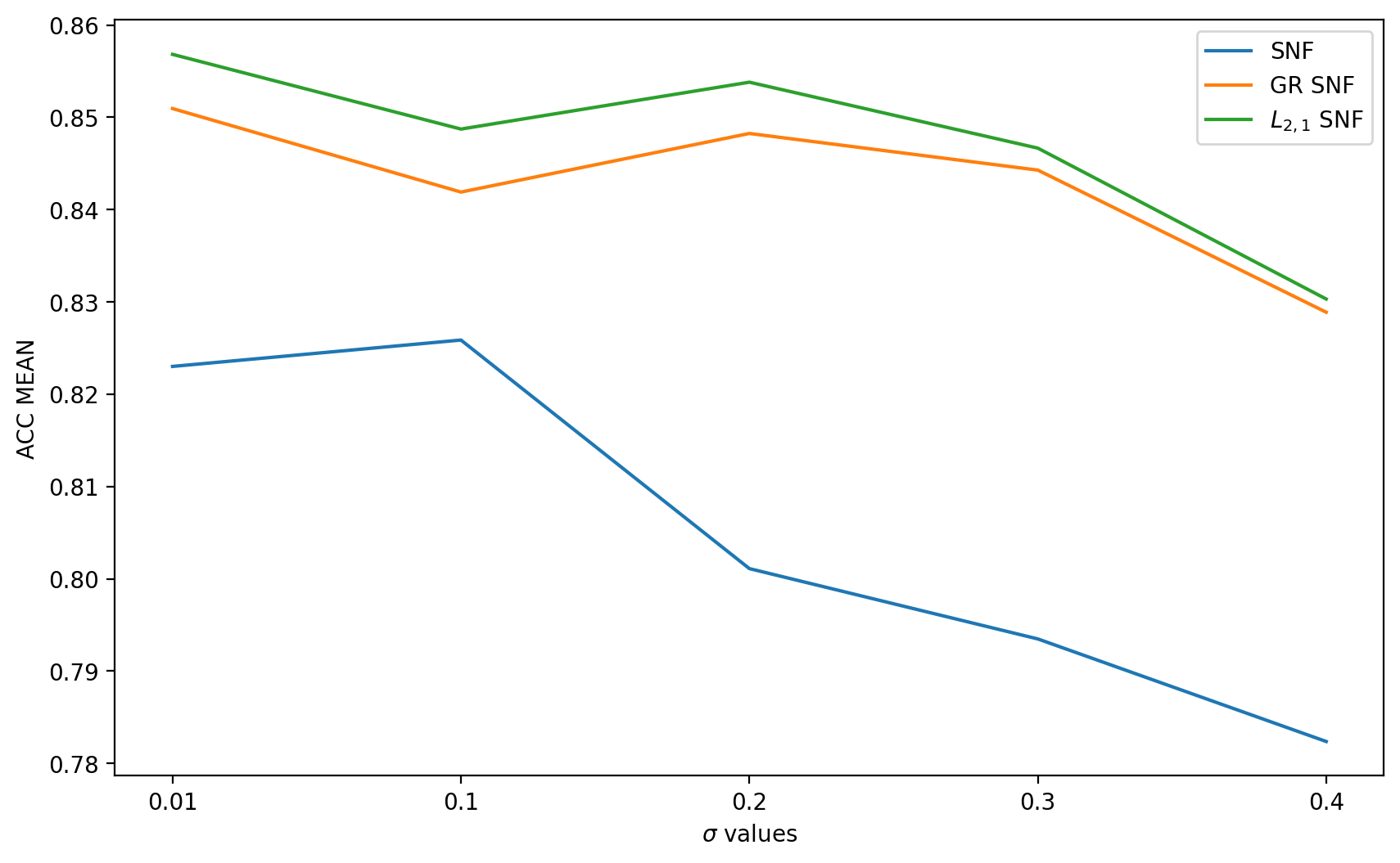
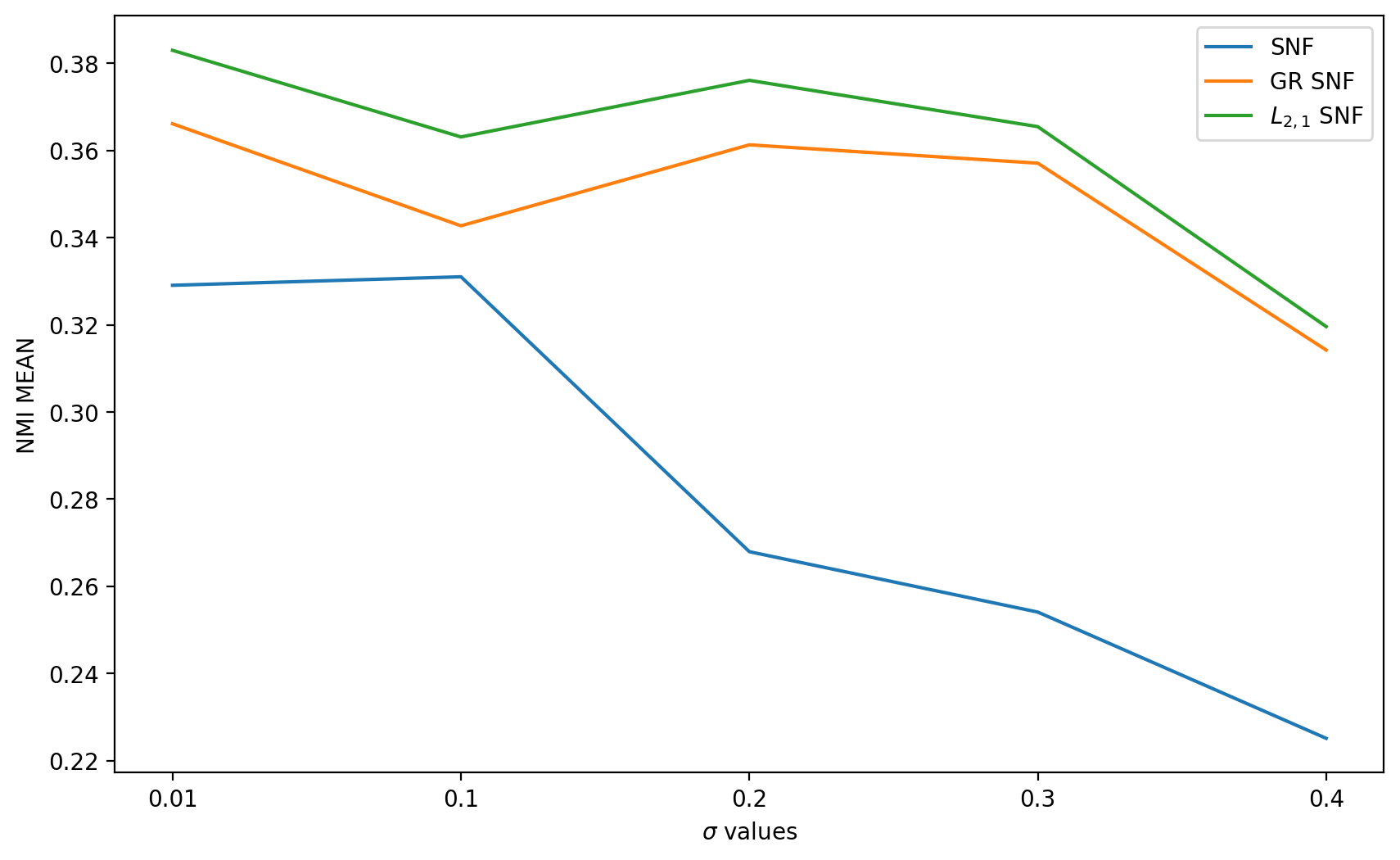
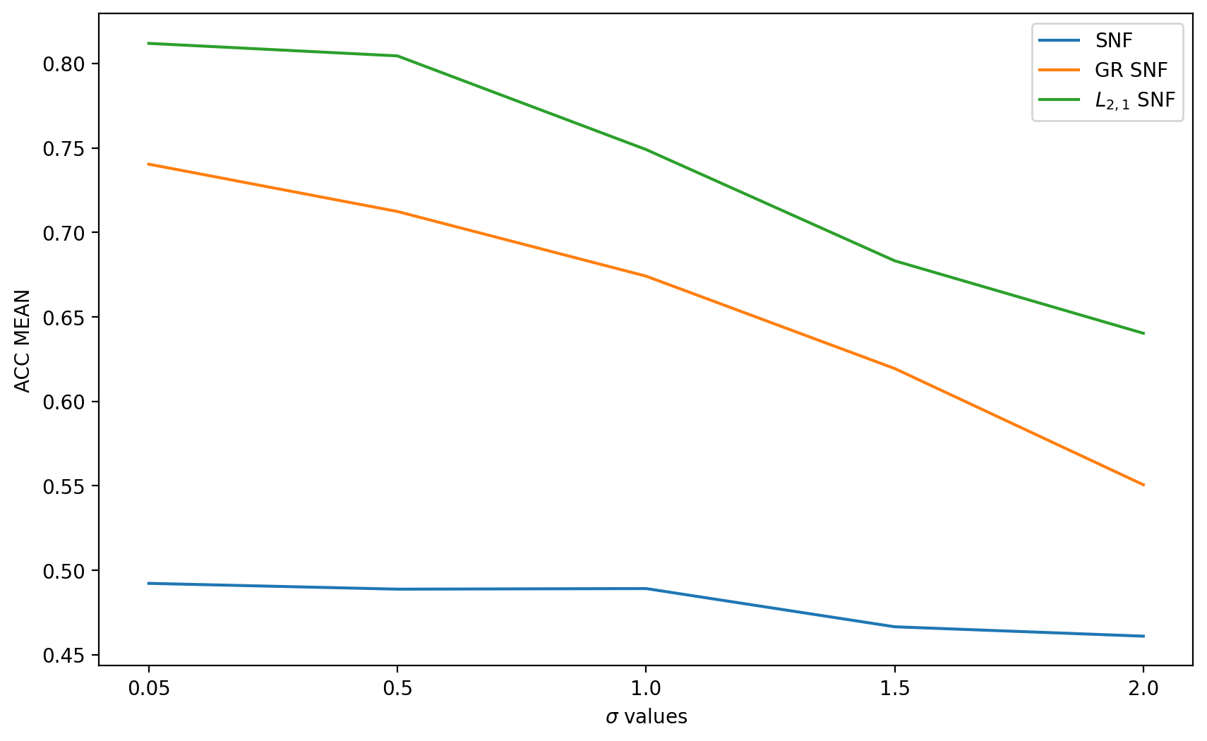
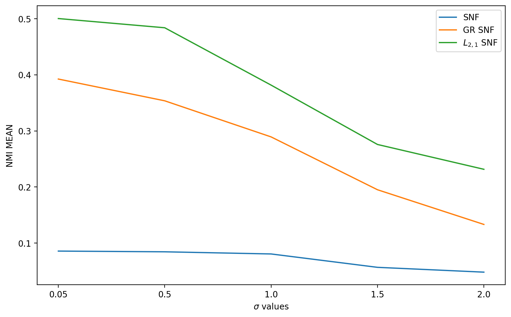
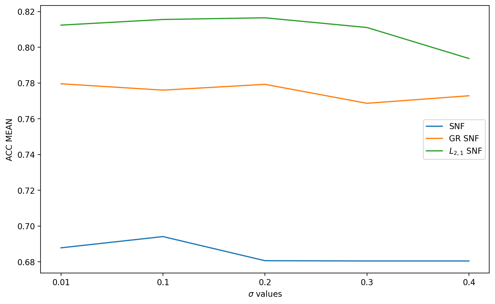
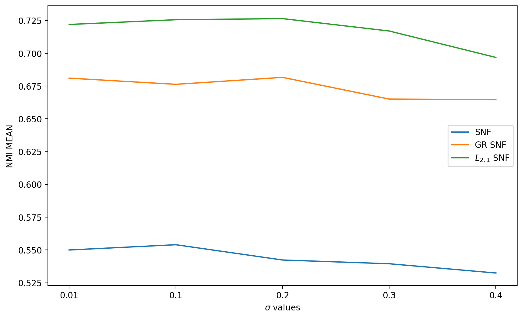
Based on these experiments, it is observed that for all the datasets, the performance of all SNF algorithms deteriorate as the noise level increases. However, SNF still outperforms SNF and GR SNF across all the datasets at different levels of Gaussian noise.
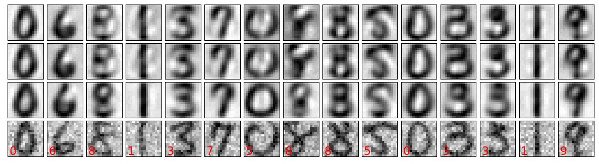
As USPST dataset is an image collection of numbers , we run an experiment with cluster number on USPST dataset which carries Gaussian noise with . The ACC and NMI means are reported as , and for SNF, GR SNF and SNF, respectively. Meanwhile, Figure 4 shows the images of randomly selected numbers reconstructed by all the algorithms as well as the original image with given Gaussian noise. It is observed that the images by SNF achieve higher precision to recapture the original images than those by the other two SNF algorithms.
4.4 Parameter Investigation for SNF
SNF has two essential parameters: measures the weight of the graph Laplacian; controls the sparse degree of the basis matrix. We investigate their influence on the ACC and NMI means for each dataset by varying and as a pair. For fairness of comparison, we choose from a wide feasible range commonly adopted in the literature and from . Once an pair is identified to achieve the best ACC and NMI means, we then conduct a refined search in the neighborhood of that pair until a new pair with better values can be found. We run the experiments with the cluster number set to for Ionosphere, for Waveform, and for USPST, respectively.
Table 5, Table 6, and Table 7 show how the ACC and NMI mean values vary with for each dataset. The optimal pair for each dataset is marked in red in each table, respectively: for Ionosphere, for Waveform, and for USPST. It is observed that all three datasets follow the same pattern: when the pair approaches towards the optimal pair from any direction, the performance of SNF improves gradually; when the pair moves away from the optimal pair, the performance of the algorithm deteriorates. Therefore, when assigned appropriate values, the graph Laplacian and the sparseness constraint are surely helpful for a better data representation.
| 0.001 | 0.01 | 0.1 | 1.0 | 10 | 100 | |
| 0.001 | (80.3,26.6) | (82.9,31.5) | (85.1,39.0) | (83.4,33.9) | (78.1,22.6) | (76.6,19.8) |
| 0.01 | (80.5,27.8) | (83.3,33.0) | (84.5,37.5) | (83.6,34.0) | (79.5,25.5) | (78.3,22.9) |
| 0.1 | (80.8,27.9) | (83.2,32.5) | (84.7,36.9) | (84.4,36.1) | (79.3,24.6) | (75.2,18.7) |
| 1.0 | (77.8,22.2) | (83.5,33.3) | (85.2,36.8) | (83.5,32.8) | (79.8,24.1) | (75.9,20.2) |
| 2.25 | (75.6,18.7) | (81.2,29.0) | (85.6,38.2) | (81.4,28.2) | (79.1,23.9) | (77.3,22.8) |
| 10 | (73.2,14.4) | (84.0,34.0) | (82.8,31.0) | (80.2,26.6) | (76.8,20.2) | (75.9,19.8) |
| 100 | (82.3,31.5) | (69.0,9.1) | (69.2,9.7) | (78.8,23.6) | (76.8,21.3) | (75.3,18.5) |
| 1000 | (75.5,18.4) | (79.8,25.6) | (79.0,24.5) | (77.1,21.4) | (76.2,20.2) | (76.0,19.5) |
| 0.001 | 0.01 | 0.1 | 1.0 | 10 | 100 | |
| 0.001 | (50.8,10.4) | (54.7,13.8) | (72.8,36.7) | (80.2,49.0) | (77.8,46.7) | (71.7,38.6) |
| 0.01 | (52.0,9.8) | (55.0,14.7) | (72.7,37.1) | (80.5,49.3) | (77.5,45.8) | (72.0,39.0) |
| 0.1 | (52.0,12.5) | (54.1,14.0) | (72.9,37.1) | (79.8,47.5) | (77.1,47.3) | (71.5,38.9) |
| 1.0 | (54.1,12.2) | (60.9,18.8) | (73.7,37.3) | (74.6,41.0) | (77.6,47.1) | (71.1,38.2) |
| 10 | (63.8,24.7) | (69.0,31.8) | (79.1,47.8) | (80.9,48.8) | (76.8,46.1) | (70.9,37.5) |
| 100 | (55.6,13.1) | (69.7,31.2) | (81.2,50.3) | (78.5,47.8) | (71.4,38.4) | (70.0,35.6) |
| 1000 | (72.8,37.1) | (80.9,49.8) | (76.5,43.8) | (62.6,23.7) | (69.3,35.6) | (70.5,35.6) |
| 0.001 | 0.01 | 0.1 | 1.0 | 10 | 100 | |
| 0.001 | (67.7,52.9) | (68.5,55.5) | (74.7,64.3) | (69.5,61.7) | (74.5,69.9) | (60.6,51.3) |
| 0.01 | (66.5,52.2) | (69.5,56.0) | (75.3,64.7) | (67.8,60.1) | (77.1,69.9) | (61.4,51.7) |
| 0.1 | (68.7,55.2) | (70.8,58.2) | (74.6,64.6) | (65.1,59.0) | (77.0,70.0) | (59.8,50.8) |
| 1.0 | (74.3,63.3) | (75.1,63.9) | (77.7,67.2) | (77.7,68.2) | (80.6,71.7) | (61.2,51.8) |
| 10 | (74.5,62.5) | (75.6,64.5) | (78.4,68.2) | (79.9,70.9) | (70.2,62.7) | (57.9,48.6) |
| 15 | (73.4,61.6) | (76.9,65.7) | (78.8,68.6) | (81.7,72.4) | (63.6,55.9) | (54.8,45.1) |
| 100 | (76.0,64.4) | (78.7,67.8) | (78.7,68.9) | (55.2,46.2) | (56.0,46.3) | (53.7,43.9) |
| 1000 | (76.9,66.0) | (61.8,54.8) | (37.3,21.9) | (59.9,50.9) | (54.2,44.1) | (52.6,42.4) |
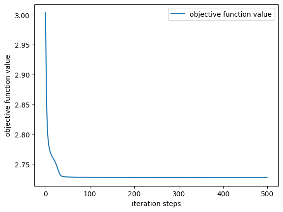
4.5 Convergence Analysis for SNF
The updating rules for minimizing the objective function of SNF are essentially iterative. We have shown that these update rules yield convergence, and we now investigate the rapidity of this convergence. To run the experiments, we set for Ionosphere, for Waveform, and for USPST, respectively. Meanwhile, the optimal pair identified in Subsection 4.4 for each dataset is adopted.
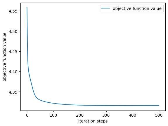
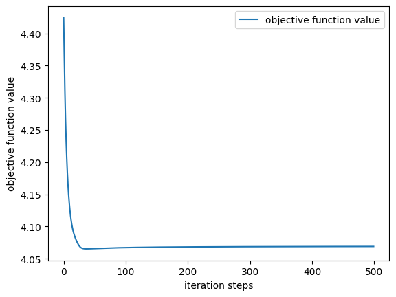
Figure 5 shows the convergence curves of SNF on all three datasets with the optimal and . For each dataset, -axis denotes the iteration number and -axis stands for the log value of the objective function. We can see that the multiplicative update rules converge very quickly, usually within dozens of iterations.
It is imperative to provide some clarification towards this experiment. Firstly, due to the small cluster size compared with the actual data size and , the leading term involving matrix decomposition error and thus the whole objective function in (11) are rather large. Secondly, since other SNF algorithms use different objective function formulas, it would be unrealistic to compare them together here. However, other algorithms also demonstrate similar rapid convergence [18, 19]. Thirdly, as there are no reported algorithms to optimize in general due to NP-hardness, the limit value found in this experiment cannot be regarded as the minimization value of (11). To further explore the relationship between the optimal value in (11) and the limit obtained by SNF algorithm, we run another experiment in Subsection 4.6 on randomized matrices where is enforced and we observe that SNF algorithm reaches the optimal value, no matter what , and their initialization are chosen randomly in advance.
4.6 Experiments on Randomized Mixed-Sign Matrices
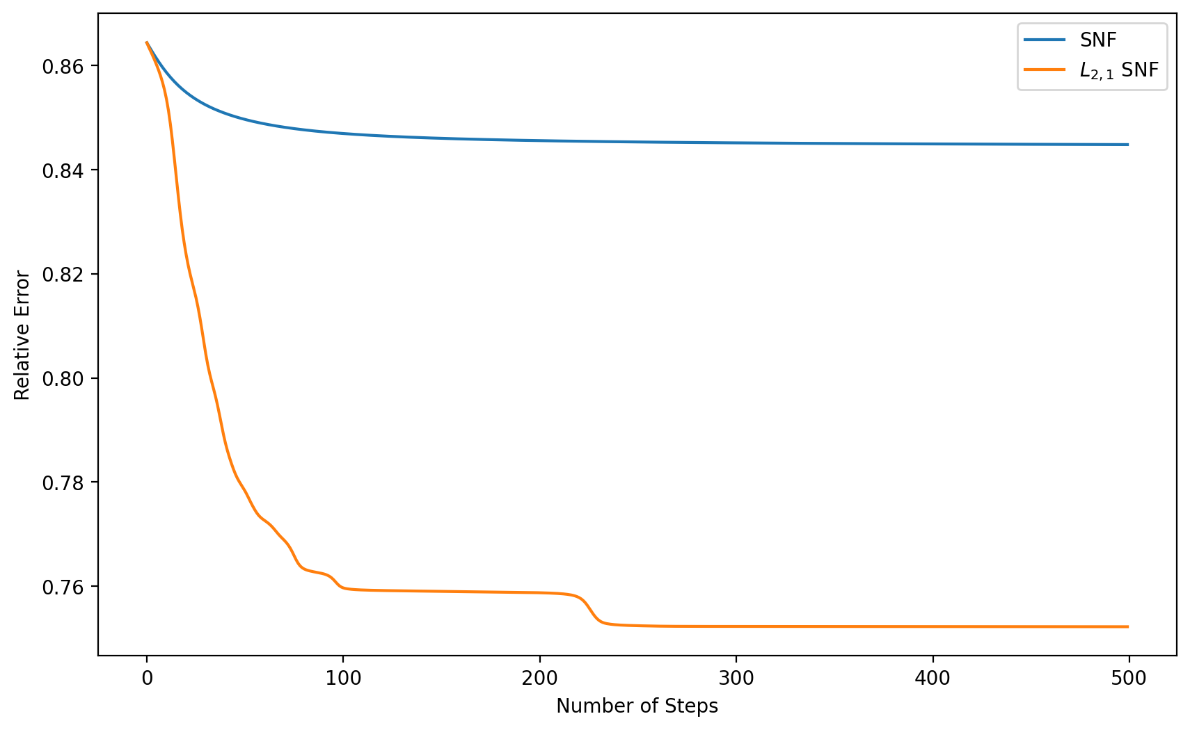
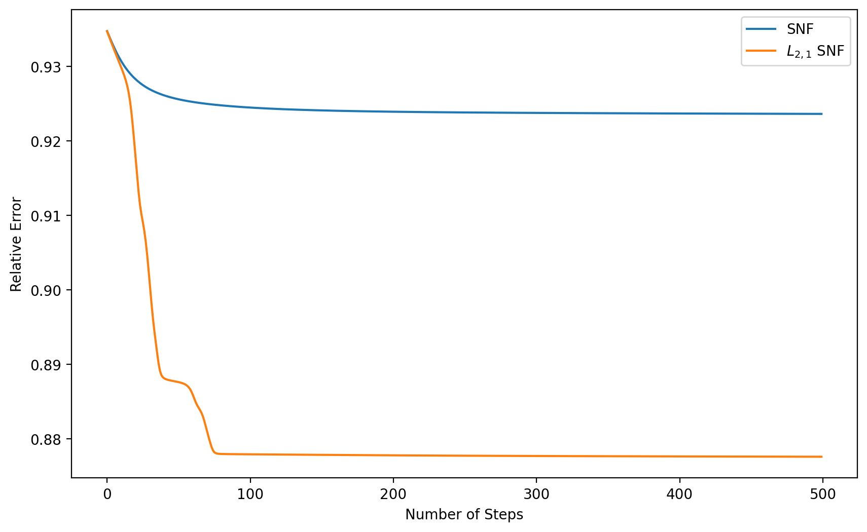
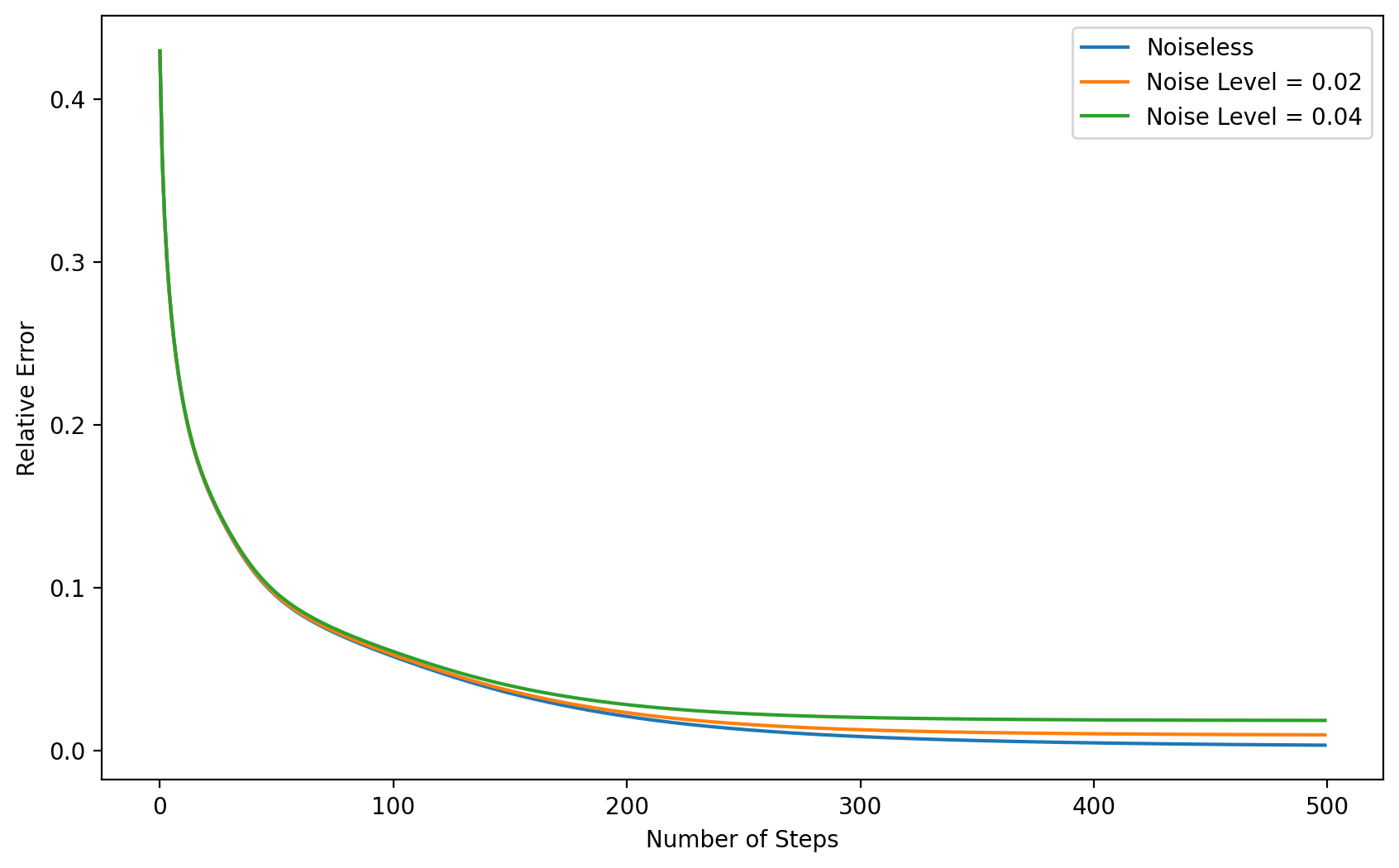
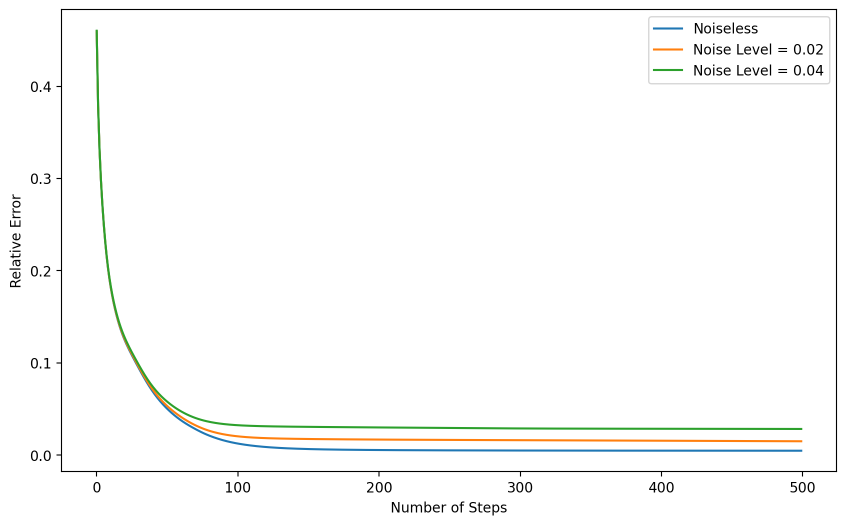
Based on the performance comparison of the parameters for SNF in Subsection 4.4, we observe that the leading term of matrix decomposition plays the most important role while the other two terms improve the algorithm performance by varying the parameters and . Therefore, for fair comparison of all SNF algorithms without the effect of tuning parameters, we set for SNF and Graph Regularized SNF, which reduces to the original SNF algorithm, and compare the numerical performance of SNF algorithm versus SNF algorithm. To this end, we begin with a randomized mixed-sign matrix of dimension in the range . We perform different degrees of size reduction with and , respectively. In fact, these extreme matrix dimensions are inspired by the potential applications towards highly over-determined systems from the text mining and genomic data compression. The initialization values of and are randomized in the range of and , respectively. We then compare the relative error , which is more suitable than the absolute error without worrying about the range of entries of , for SNF and SNF algorithms at different iteration steps.
Overall, SNF algorithm demonstrates a substantial improvement over SNF algorithm in reducing the relative errors, as shown in Figure 6.
Since it is unclear whether NMF and SNF algorithms converge to global minimizers of the objective functions theoretically, it is necessary to investigate how close their solutions are to the global minimizers in practice. Therefore, we run another experiment for SNF algorithm where of dimension and of dimension are generated randomly in the range of and , respectively for the cases of and . We then enforce of dimension so that the objective function can indeed reach for all the cases. The initialization values for and are still randomized in the range of and , respectively. Furthermore, we add Gaussian noise at different levels with (noiseless), and to observe the robustness of SNF algorithm. We then compare the relative error at different iteration steps. The experimental results in Figure 7 show that without Gaussian noise, the objective function always converges to the optimal value , irrespective of the randomized initial values of and . When the level of Gaussian noise increases, the error becomes larger but still stays within a reasonable range around . In fact, original SNF algorithm also shows similar numerical behavior but we skip it here for brevity. This experiment confirms reported robustness of SNF algorithms. It also necessitates theoretical investigation on whether such limits from SNF algorithms can reach .
4.7 Experiments on CIFAR-10 Image Dataset
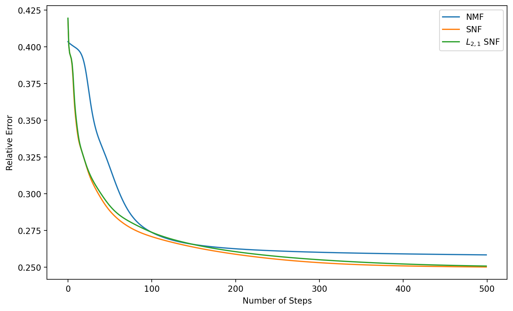
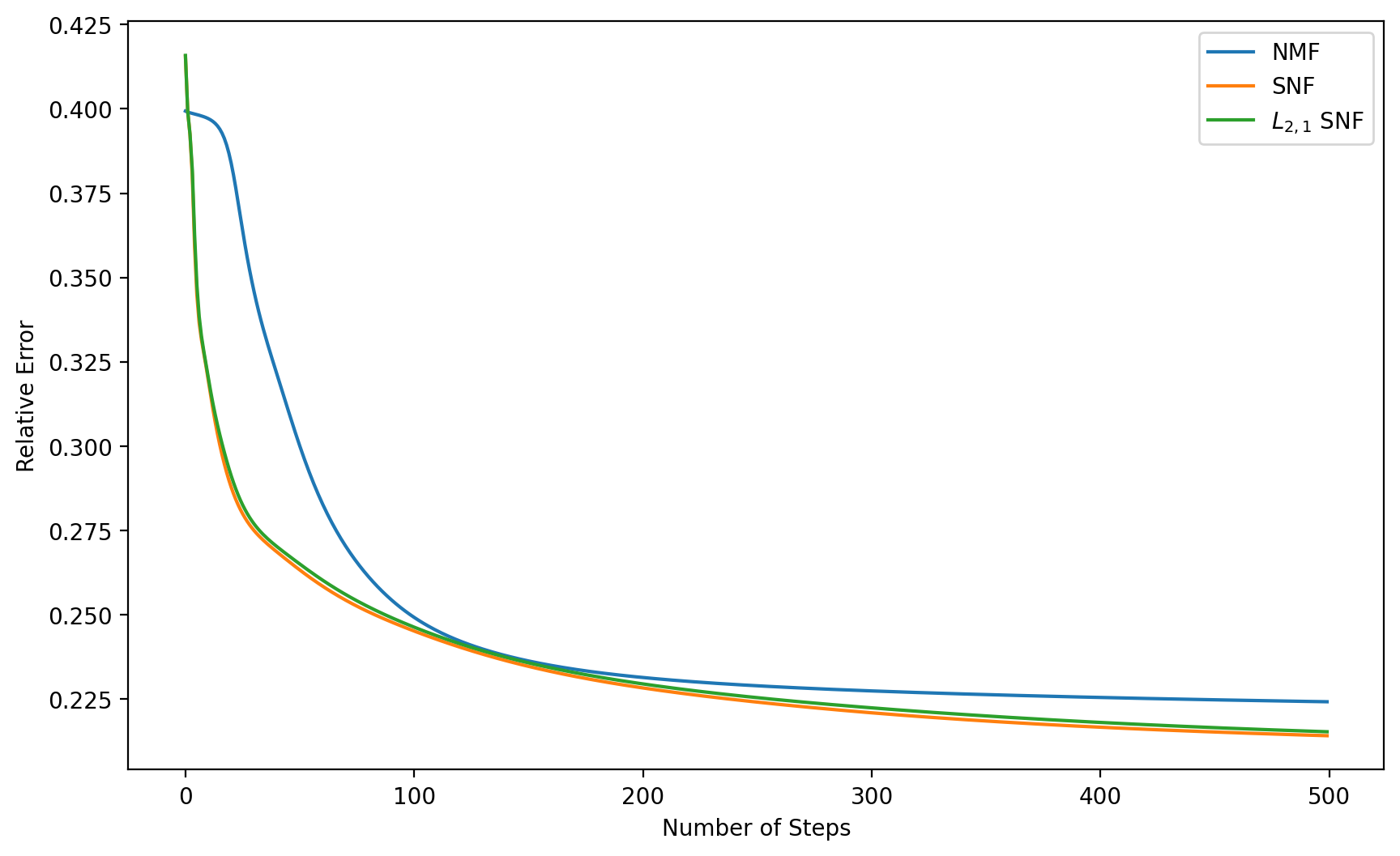
There exists many large-scale benchmark datasets used to measure the performance of new algorithms, such as CIFAR-10, Fashion-MNIST, etc. All such datasets turn out to contain nonnegative data which is the most popular data format in the field of machine learning. We now conduct a new experiment on the CIFAR-10 dataset which consists of 50000 training images and 10000 test images in 10 classes with corresponding labels in the range of . Each image is a color image under the RGB color model and can thus be represented by a column vector of size whose entries are in the range of . We construct a matrix of size to represent the whole set of test images by columns and then apply NMF algorithm (4), SNF algorithm (7), and SNF algorithm with (12) towards decomposition of . We perform different degrees of size reduction with and , respectively. The initialization values of and are randomized in the range of . We compare the relative error for all the algorithms at different iteration steps.
As we know, SNF algorithms (7) and (12) are designed exclusively for mixed-sign data decomposition. Then for the nonnegative image matrix , SNF algorithms yield mixed-sign matrix and may lead to undesired data reconstruction of the images due to existence of negative values, while NMF algorithm (4) works seamlessly due to its constraint. Therefore, it would be unrealistic to compare ACC and NMI based on the coordinate matrix . Nevertheless, it is still reasonable to compare their relative errors to observe which algorithm yields the best approximation of .
As shown in Figure 8, SNF and SNF algorithms demonstrate better performance than NMF algorithm in reducing the relative errors. Meanwhile, SNF shows similar performance as original SNF as the proposed noise reduction mechanism is developed towards mixed-sign data. Therefore, this experiment verifies robustness of SNF algorithm (12) in approximation of nonnegative datasets although it is designed for mixed-sign data.
5 Conclusion and Future Research
We have presented a novel data reduction algorithm, SNF, which renders a parts-based compression of mixed-sign data while reducing the effects of noise and outliers. We provide theoretical proof of monotonic convergence of the iterative updates given by the algorithm. Through experiments on three benchmark mixed-sign datasets and several randomized matrices with different levels of Gaussian noise, we demonstrate the advantage of SNF over other conventional SNF algorithms. In our future work, we will investigate theoretically the relationship between the solutions obtained by SNF algorithms and the global optimizers of the objective functions. We will also incorporate prior discriminative label information within SNF to construct a semi-supervised algorithm which is better-suited for real-world applications, including data mining and image processing.
Acknowledgement
The authors thank the two anonymous reviewers and the editor for their useful suggestions which significantly improve the quality of this paper. This work is partially supported by NSF Research Training Group Grant DMS-2136228.
Conflict of Interest Statement
The authors declare that they have no conflict of interest.
References
- [1] Hariharan Narayanan and Sanjoy Mitter. Sample complexity of testing the manifold hypothesis. In Advances in Neural Information Processing Systems 23, pages 1786–1794, 2010.
- [2] Deguang Kong, Chris Ding, and Heng Huang. Robust nonnegative matrix factorization using l21-norm. In Proceedings of the 20th ACM International Conference on Information and Knowledge Management, pages 673–682, 2011.
- [3] Daniel Lee and Sebastian Seung. Algorithms for non-negative matrix factorization. In Advances in Neural Information Processing Systems 13, pages 556–562, 2001.
- [4] Chih-Jen Lin. On the convergence of multiplicative update algorithms for nonnegative matrix factorization. IEEE Transactions on Neural Networks, 18:1589–1596, 2007.
- [5] Daniel Lee and Sebastian Seung. Learning the parts of objects by non-negative matrix factorization. Nature, 401:788–791, 1999.
- [6] Chih-Jen Lin. Projected gradient methods for nonnegative matrix factorization. Neural Computation, 19:2756–2779, 2007.
- [7] Hyunsoo Kim and Haesun Park. Nonnegative matrix factorization based on alternating nonnegativity constrained least squares and active set method. SIAM Journal on Matrix Analysis and Applications, 30:713–730, 2008.
- [8] Hongwei Liu, Xiangli Li, and Xiuyun Zheng. Solving non-negative matrix factorization by alternating least squares with a modified strategy. Data Mining and Knowledge Discovery, 26:435–451, 2013.
- [9] Deng Cai, Xiaofei He, Jiawei Han, and Thomas Huang. Graph regularized nonnegative matrix factorization for data representation. IEEE Transactions on Pattern Analysis and Machine Intelligence, 33(8):1548–1560, 2011.
- [10] Patrik Hoyer. Non-negative matrix factorization with sparseness constraints. Journal of Machine Learning Research, 5:1457–1469, 2004.
- [11] Feiping Nie, Heng Huang, Xiao Cai, and Chris Ding. Efficient and robust feature selection via joint l2,1-norms minimization. In Advances in Neural Information Processing Systems 23, pages 1813–1821, 2010.
- [12] Yi Yang, Hengtao Shen, Zhigang Ma, Zi Huang, and Xiaofang Zhou. L2,1-norm regularized discriminative feature selection for unsupervised learning. In Proceedings of the 22th International Joint Conference on Artificial Intelligence, pages 1589–1594, 2011.
- [13] Baolei Wu, Enyuan Wang, Zhen Zhu, Wei Chen, and Pengcheng Xiao. Manifold nmf with l21 norm for clustering. Neurocomputing, 273:78–88, 2018.
- [14] Hyekyoung Lee, Jiho Yoo, and Seungjin Choi. Semi-supervised nonnegative matrix factorization. IEEE Signal Processing Letters, 17:4–7, 2010.
- [15] Zhiwei Xing, Yingcang Ma, Xiaofei Yang, and Feiping Nie. Graph rregularized nonnegative matrix factorization with label discrimination for data clustering. Neurocomputing, 440:297–309, 2021.
- [16] Cuina Jiao, Yinglian Gao, Na Yu, Jinxing Liu, and Lianyong Qi. Hyper-graph regularized constrained nmf for selecting differentially expressed genes and tumor classification. IEEE Journal of Biomedical and Health Informatics, 24:3002–3011, 2020.
- [17] Na Yu, Mingjuan Wu, Jinxing Liu, Chunhou Zheng, and Yong Xu. Correntropy-based hypergraph regularized nmf for clustering and feature selection on multi-cancer integrated data. IEEE Transactions on Cybernetics, 51:3952–3963, 2021.
- [18] Chris Ding, Tao Li, and Michael Jordan. Convex and semi-nonnegative matrix factorizations. IEEE Transactions on Pattern Analysis and Machine Intelligence, 32:45–55, 2010.
- [19] Peng Luo and Jinye Peng. Group sparsity and graph regularized semi-nonnegative matrix factorization with discriminability for data representation. Entropy, 19:627, 2017.
- [20] Zhenqiu Shu, Xiaojun Wu, Cong Hu, Congzhe You, and Honghui Fan. Deep semi-nonnegative matrix factorization with elastic preserving for data representation. Multimedia Tools and Applications, 80:1707–1724, 2021.
- [21] Wei Jiang, Tingting Ma, Xiaoting Feng, Yun Zhai, Kewei Tang, and Jie Zhang. Robust semi-nonnegative matrix factorization with adaptive graph regularization for gene representation. Chinese Journal of Electronics, 29:122–131, 2020.
- [22] Florian Rousset, Françoise Peyrin, and Nicolas Ducros. A semi nonnegative matrix factorization technique for pattern generalization in single-pixel imaging. IEEE Transactions on Computational Imaging, 4:284–294, 2018.
- [23] Chong Peng, Zhilu Zhang, Chenglizhao Chen, Zhao Kang, and Qiang Cheng. Two-dimensional semi-nonnegative matrix factorization for clustering. Information Sciences, 590:106–141, 2022.
- [24] Stephen Vavasis. On the complexity of nonnegative matrix factorization. SIAM Journal on Optimization, 20:1364–1377, 2010.
- [25] Nicolas Gillis and Abhishek Kumar. Exact and heuristic algorithms for semi-nonnegative matrix factorization. SIAM Journal on Matrix Analysis and Applications, 36:1404–1424, 2015.
- [26] Nicolas Gillis. Nonnegative matrix factorization. SIAM Data Science Book Series, pages 1–350, 2020.
- [27] Dimitris Chachlakis, Ashley Prater-Bennette, and Panos Markopoulos. L1-norm tucker tensor decomposition. IEEE Access, 7:178454–178465, 2019.
- [28] Bo Jiang and Chris Ding. Revisiting l2,1-norm robustness with vector outlier regularization. IEEE Transactions on Neural Networks and Learning Systems, 31:5624–5629, 2020.
- [29] Jorge Nocedal and Stephen Wright. Numerical optimization. Springer Series in Operations Research and Financial Engineering, pages 1–686, 2006.