Policies with Sparse Inter-Agent Dependencies in Dynamic Games: A Dynamic Programming Approach

Abstract.

Common feedback strategies in multi-agent dynamic games require all players’ state information to compute control strategies. However, in real-world scenarios, sensing and communication limitations between agents make full state feedback expensive or impractical, and such strategies can become fragile when state information from other agents is inaccurate. To this end, we propose a regularized dynamic programming approach for finding sparse feedback policies that selectively depend on the states of a subset of agents in dynamic games. The proposed approach solves convex adaptive group Lasso problems to compute sparse policies approximating Nash equilibrium solutions. We prove the regularized solutions’ asymptotic convergence to a neighborhood of Nash equilibrium policies in linear-quadratic (LQ) games. We extend the proposed approach to general non-LQ games via an iterative algorithm. Empirical results in multi-robot interaction scenarios show that the proposed approach effectively computes feedback policies with varying sparsity levels. When agents have noisy observations of other agents’ states, simulation results indicate that the proposed regularized policies consistently achieve lower costs than standard Nash equilibrium policies by up to 77% for all interacting agents whose costs are coupled with other agents’ states.

1. Introduction

Dynamic game theory models the strategic decisions of multiple interacting agents over time. In such games, it is common to identify solutions at which players execute full state feedback strategies that depend on all players’ states. For example, in multi-robot formations, each robot typically plans its actions based on the states of other robots. However, obtaining full state information is often expensive or impractical due to sensing and communication limitations. Worse, dense strategies that require access to many other agents’ states can be brittle when such state information is inaccurate, e.g., in the presence of uncertainties. Consequently, it is desirable for agents to find strategies that selectively depend on the states of a subset of agents while still approximating equilibrium behavior.

We contribute an algorithm for finding sparse feedback policies that depend on fewer influential agents’ states in dynamic games while approximating Nash equilibrium strategies. More specifically, we propose a regularized dynamic programming (DP) scheme Başar and Olsder (1998); Bertsekas (2012) that approximately solves LQ dynamic games, which are an important extension of the linear-quadratic regulator (LQR) problem Kalman et al. (1960) to multi-agent interaction settings. The proposed approach solves a convex adaptive group Lasso regularization problem Wang and Leng (2008) to encode structured sparsity within each DP iteration. A user can choose a desired sparsity level based on the available sensing or communication resources. We also employ an iterative linear-quadratic approximation technique Fridovich-Keil et al. (2020); Laine et al. (2021) to extend the proposed approach to general non-LQ games.

To establish theoretical properties of the proposed approach, we first derive an upper bound on the deviation of the regularized policy matrix computed by the proposed approach from the Nash equilibrium in a single stage of an LQ game. Then, we prove the asymptotic convergence of the regularized DP recursion to a neighborhood of the Nash equilibrium across all stages of the game.

We empirically test the proposed approach in simulation and support the following key claims: First, the proposed approach yields more sparse feedback strategies than standard Nash equilibrium solutions and thereby requires less communication and sensing resources to execute. Second, the proposed approach yields different levels of sparsity as the user varies the regularization strength. Third, we empirically show that the proposed approach can be readily extended to general non-LQ games via an iterative scheme. Fourth, for all interacting agents whose costs are coupled with other agents’ states, the regularized strategies show improved robustness and task performance in comparison to standard Nash equilibria in cases where agents only have inaccurate knowledge of other agents, e.g., noisy estimates of other agents’ states.

2. Related Works

2.1. Noncooperative Games

Over the years, a growing body of literature has explored the application of dynamic noncooperative games Başar and Olsder (1998); Isaacs (1999) in designing autonomous systems Schwarting et al. (2019); Fridovich-Keil et al. (2020); Fisac et al. (2019); Wang et al. (2021); Mehr et al. (2023); Yu et al. (2023); Peters et al. (2023); Liu et al. (2024); Li et al. (2023); Hu et al. (2024); Gupta et al. (2024). Among different types of games, we focus on general-sum Nash equilibrium problems, where players can have partially competing objectives and make decisions simultaneously. In Nash games with different information patterns, feedback and open-loop Nash equilibrium are the most common solution types. Open-loop Nash equilibria ignore the dynamic, multi-stage nature of the problem by assuming that players choose their entire decision sequences, i.e., trajectories, at once Cleac’h et al. (2022); Zhu and Borrelli (2023); Facchinei and Pang (2003); Liu et al. (2023); Peters et al. (2024). In contrast, a feedback Nash equilibrium is a set of control policies that map game states to players’ controls; they are more expressive than open-loop solutions but strictly more challenging to compute. Various special cases have been studied, e.g., in Reddy and Zaccour (2017); Tanwani and Zhu (2020); Kossioris et al. (2008), among others. For general feedback games with nonconvex costs and constraints, only approximate solutions exist, e.g., in Fridovich-Keil et al. (2020); Laine et al. (2021). We also note that both open-loop and feedback LQ games have well-studied solutions Başar and Olsder (1998); Li and Gajic (1995).

This work focuses on feedback solutions to LQ dynamic games, where we encourage sparsity structure in the resulting strategies via a regularized DP procedure. We also extend the approach to non-LQ games via an iterative linear-quadratic approximation technique Fridovich-Keil et al. (2020).

2.2. Structured Controller Design

The literature on encoding sparsity structures into control strategies primarily focuses on single-agent optimal control settings Kalman et al. (1960) and can generally be categorized into two groups. The first category Wenk and Knapp (1980); Lin et al. (2011); Mårtensson and Rantzer (2012); Lamperski and Lessard (2012); Fardad et al. (2009); Furieri et al. (2020) requires a predefined sparsity structure, using this as a constraint to compute controls. For instance, each controller may have access only to a subset of the sensing information. More relevant to our work, studies in the second category propose methods to encourage sparsity in classical LQR problems without requiring a predefined sparsity structure Lin et al. (2013); Dörfler et al. (2014); Wytock and Kolter (2013); Park et al. (2020). These approaches introduce sparsity regularizers into the LQR cost, resulting in nonconvex policy optimization problems. Within this group, some studies further attempt to encourage sparse policies in cooperative Markov games with finite state-action spaces Karabag et al. (2022) and continuous noncooperative LQ games Lian et al. (2017). While the work in Lian et al. (2017) simply applies a policy optimization method for each player independently, noncooperative multi-agent scenarios require extra caution. Policy optimization is known to be a challenging nonconvex problem even in the settings of the LQR Fazel et al. (2018); Malik et al. (2020) and zero-sum games Zhang et al. (2019); Bu et al. (2019) without sparsity regularization. Worse, policy gradient approaches can generally be non-convergent in general-sum noncooperative settings, even in LQ games Mazumdar et al. (2020).

Research on finding sparse policies in noncooperative games remains relatively scarce, despite the fact that sparse strategies are especially desirable in reducing inter-agent communication and sensing requirements. To address this gap, our approach encourages group sparsity in the computed control policies, where each group corresponds to the influence of one agent’s state on another agent’s control action. Given the convergence challenges associated with direct policy optimization in general-sum games, we adopt a modified DP approach. At each stage, we solve a convex adaptive group Lasso problem Wang and Leng (2008); Yuan and Lin (2006), an extension of the Lasso problem Tibshirani (1996) to variables in pre-specified groups. This modified DP scheme retains convexity and enables formal convergence analysis and extension to more general non-LQ game settings.

3. Preliminaries

We study non-cooperative dynamic games played by $N$ players in discrete time $t\in\{1,\dots,T\}\equiv[T]$; players follow a joint dynamical system:

$$x_{t+1}=f_{t}(x_{t},u^{1}_{t},\ldots,u^{N}_{t}),$$ (1)

where $x$ and $u$ denote players’ states and controls. Superscripts denote players’ indices and subscripts are discrete time steps, e.g., $u_{t}^{i}$ denotes player $i$’s control at time step $t$. Throughout the manuscript, the absence of player and time indices without additional definition denotes concatenation, i.e., $x_{t}:=[x^{1\top}_{t},x^{2\top}_{t},\ldots,x^{N\top}_{t}]^{\top}$ and $x^{i}:=[x^{i\top}_{1},x^{i\top}_{2},\ldots,x^{i\top}_{T}]^{\top}$. Each player $i\in\{1,\dots,N\}\equiv[N]$ seeks to minimize their own cost $J^{i}$:

$$\min_{u^{i}}\underbrace{\sum_{t=1}^{T}g_{t}(x_{t},u^{1}_{t},\ldots,u^{N}_{t})+g_{T+1}(x_{T+1})}_{J^{i}(u_{1},\dots,u_{T})},$$ (2)

consisting of additive stage costs $g_{t},\forall t\in[T]$ and a terminal cost $g_{T+1}$. The initial state of the game $x_{1}$ is a given a priori. In particular, we focus on LQ games which we introduce below; we discuss an extension to more general non-LQ games in Section 4.2.

Definition 0.

An N-player, general-sum, discrete-time dynamic game is a linear-quadratic (LQ)game if players’ costs are quadratic:

$$\begin{aligned} J^{i}=\frac{1}{2}\sum_{t=1}^{T}\Big{(}(x_{t}^{\top}Q_{t}^{i}+2q_{t}^{i\top})x_{t}+\sum_{j=1}^{N}(u_{t}^{j\top}R_{t}^{ij}+2r_{t}^{ij\top})u_{t}^{j}\Big{)}\\ +\frac{1}{2}(x_{T+1}^{\top}Q_{T+1}^{i}+2q_{T+1}^{i\top})x_{T+1},\end{aligned}$$ (3)

and dynamics are linear:

$$x_{t+1}=A_{t}x_{t}+\sum_{i=1}^{N}B_{t}^{i}u_{t}^{i},$$ (4)

with $x_{t}^{i}\in\mathbb{R}^{m^{i}},u_{t}^{i}\in\mathbb{R}^{n^{i}}$, and $Q_{t}^{i}\succeq 0,R^{ii}_{t}\succ 0,\forall i\in[N]$. We let $m=\sum_{i\in[N]}m^{i}$ and $n=\sum_{i\in[N]}n^{i}$.

We focus on the solution concept of feedback Nash equilibrium (Başar and Olsder, 1998, Def. 6.2) defined below.

Definition 0.

A feedback Nash equilibrium of an N-player, general-sum, discrete-time dynamic game is an $N$-tuple of strategies $\{\gamma^{i*},i\in[N]\}$ with $u_{t}^{i*}=\gamma_{t}^{i*}(x_{t})$ that satisfies the following Nash equilibrium conditions $\forall t\in[T],i\in[N]$ for the cost in Eq. 2:

$$J^{i}\bigg{(}(\gamma^{j}_{v})_{j=1,v=1}^{N,t-1},(\gamma^{j*}_{v})_{j=1,v=t}^{N,T}\bigg{)}$$ (5)

$$\leq J^{i}\bigg{(}\underbrace{(\gamma^{j}_{v})_{j=1,v=1}^{N,t-1}}_{\mathrm{stages}<t},\underbrace{\Big{(}(\gamma^{j*}_{v})_{j\neq i,v=t}^{T},\big{(}(\gamma^{i}_{v})_{v=t},(\gamma^{i*}_{v})_{v=t+1}^{T}\big{)}\Big{)}}_{\mathrm{stages}\geq t}\bigg{)}.$$

Intuitively, at a feedback Nash equilibrium, each player’s strategy is unilaterally optimal from an arbitrary stage $t$ onwards. We note that the standard feedback Nash equilibrium in Definition 2 consists of full-state feedback strategies $\gamma_{t}^{i*}$ that map all players’ states to player $i$’s control $u_{t}^{i*}=\gamma_{t}^{i*}(x_{t})$. This work seeks to find regularized feedback Nash equilibrium strategies that approximate standard Nash equilibrium and also are sparse, i.e., depend on fewer agents’ states.

4. Approach

Section 4.1 presents the proposed approach to compute regularized feedback Nash equilibria in LQ games, which is the focus of this work. Section 4.2 discusses an extension to non-LQ games.

4.1. Regularized Dynamic Programming for Linear-Quadratic Games

We first derive the computation of standard feedback Nash equilibria and then discuss the modification to yield regularized solutions.

4.1.1. Computation of Feedback Nash Equilibrium via DP

A feedback Nash equilibrium solution recursively satisfies the following coupled Hamilton–Jacobi (HJ) equations for value functions $V_{t}^{i}(x_{t})$ Başar and Olsder (1998); Fridovich-Keil (2024), $\forall i\in[N],t\in[T]$:

$$V_{t}^{i}(x_{t})=$$ (6)

$$\min_{u_{t}^{i}}\Big{(}\underbrace{\frac{1}{2}(x_{t}^{\top}Q_{t}^{i}+2q_{t}^{i\top})x_{t}+\frac{1}{2}\sum_{j=1}^{N}(u_{t}^{j\top}R_{t}^{ij}+2r_{t}^{ij\top})u_{t}^{j}+V_{t+1}^{i}(x_{t+1})}_{l_{t}^{i}(x_{t},u_{t})}\Big{)},$$

where other agents play their Nash equilibrium strategies, i.e., $u^{j}_{t}=\gamma^{j*}(x_{t}),\forall j\neq i$; $V_{T+1}^{i}(x_{T+1})$ is equal to the terminal cost $\frac{1}{2}(x_{T+1}^{\top}Q_{T+1}^{i}+2q_{T+1}^{i\top})x_{T+1}$.

We start from the final stage $t=T$ and conduct a dynamic programming procedure backward. We first plug $V_{T+1}^{i}(x_{T+1})$ into LABEL:eq:hj:

$$V_{T}^{i}(x_{T})=\min_{u_{T}^{i}}\bigg{(}\frac{1}{2}(x_{T}^{\top}Q_{T}^{i}+2q_{T}^{i\top})x_{T}+\frac{1}{2}\sum_{j=1}^{N}(u_{T}^{j\top}R_{T}^{ij}+2r_{T}^{ij\top})u_{T}^{j}$$ (7)

$$+\frac{1}{2}\Big{(}(A_{T}x_{t}+\sum_{j=1}^{N}B^{j}_{T}u_{T}^{j})^{\top}Q_{T+1}^{i}+2q_{T+1}^{i\top}\Big{)}(A_{T}x_{T}+\sum_{j=1}^{N}B^{j}_{T}u_{T}^{j})\bigg{)}.$$

Hence, Eq. 7 yields a static game for $t=T$. In fact, we will see later that each stage of LABEL:eq:hj results in a static game, and the dynamic game of interest nests the stages together. Under the assumption $Q_{t}^{i}\succeq 0,R^{ii}_{t}\succ 0,R^{ij}_{t}\succeq 0,\forall i,j\in[N],i\neq j$, $l_{T}^{i}(x_{T},u_{T})$ is strongly convex in $u_{T}^{i}$, and therefore first-order necessary conditions are sufficient for optimality. By setting the gradient $\nabla_{u_{T}^{i}}l_{T}^{i}=0$, we obtain:

$$0 =\nabla_{u_{T}^{i}}l_{T}^{i}(x_{T},u_{T})$$ (8)

$$=R_{T}^{ii}u^{i*}_{T}+r_{T}^{ii}+B^{i\top}_{T}Q_{T+1}^{i}(A_{T}x_{T}+\sum_{j=1}^{N}B^{j}_{T}u_{T}^{j*})+B_{T}^{i\top}q_{T+1}^{i},$$

from which we can conclude that the feedback Nash equilibrium policy takes a linear form:

$$u_{T}^{i*}=\gamma_{T}^{i*}(x_{T})=-P_{T}^{i}x_{T}-\alpha_{T}^{i}.$$ (9)

We refer to $P^{i}_{T}$ as a policy matrix, to which we are interested in encoding group sparsity in Section 4.1.2. Plugging the linear feedback policy in Eq. 9 into the value function in Eq. 7, we can see that, when $t=T$, the value function takes a quadratic form:

$$V_{t}^{i}(x_{t})=\frac{1}{2}(x_{t}^{\top}Z_{t}^{i}+2\eta_{t}^{i\top})x_{t}+\beta_{t}^{i},$$ (10)

with $Z_{t}^{i},\eta_{t}^{i},\beta_{t}^{i}$ being defined recursively:

$$Z_{t}^{i}=Q_{t}^{i}+\sum_{j=1}^{N}P_{t}^{j\top}R_{t}^{ij}P_{t}^{j}+F_{t}^{\top}Z^{i}_{t+1}F_{t}$$ (11)

$$\eta_{t}^{i}=q_{t}^{i}+\sum_{j=1}^{N}(P_{t}^{j\top}R_{t}^{ij}\alpha_{t}^{j}-P_{t}^{j\top}r_{t}^{ij})+F_{t}^{\top}(Z_{t+1}^{i}\omega_{t}+\eta_{t+1}^{i})$$

$$\beta_{t}^{i}=\frac{1}{2}(\alpha_{t}^{j\top}R_{t}^{ij}-2r_{t}^{ij\top})\alpha_{t}^{j}+\frac{1}{2}(Z_{t+1}^{i}\omega_{t}+2\eta_{t+1}^{i})^{\top}\omega_{t}+\beta_{t+1}^{i},$$

where:

$$F_{t}=A_{t}-\sum_{j=1}^{N}B^{j}_{t}P^{j}_{t},\omega_{t}=-\sum_{j=1}^{N}B^{j}_{t}\alpha_{t}^{j}$$

$$Z^{i}_{T+1}=Q^{i}_{T+1},\eta_{T+1}^{i}=q_{T+1}^{i}.$$

We refer to $Z_{t}^{i}$ as a value matrix.

The value function $V_{t}^{i}(x_{t})$ is also defined by the Nash equilibrium policy $\gamma_{t}^{i*}$, which we can compute by solving the linear system of equations formed by plugging Eq. 9 into Eq. 8:

$$(R_{t}^{ii}+B_{t}^{i\top}Z_{t+1}^{i}B_{t}^{i})P_{t}^{i}+B_{t}^{i\top}Z_{t+1}^{i}\sum_{j\neq i}B^{j}_{t}P_{t}^{j}=B_{t}^{i\top}Z_{t+1}^{i}A_{t},$$ (12a)

$$(R_{t}^{ii}+B_{t}^{i\top}Z_{t+1}^{i}B_{t}^{i})\alpha_{t}^{i}+B_{t}^{i\top}Z_{t+1}^{i}\sum_{j\neq i}B^{j}_{t}\alpha_{t}^{j}=B_{t}^{i\top}\eta_{t+1}^{i}+r_{t}^{ii}.$$ (12b)

We rewrite Eq. 12a in a matrix form $S_{t}P_{t}=Y_{t}$, which we shall use in Section 4.1.2:

$$\begin{aligned} \underbrace{\begin{bmatrix}R_{t}^{11}+B_{t}^{1\top}Z_{t+1}^{1}B_{t}^{1}&.&\ldots&B_{t}^{1\top}Z_{t+1}^{1}B_{t}^{N}\\ B_{t}^{2\top}Z_{t+1}^{2}B_{t}^{1}&.&\ldots&B_{t}^{2\top}Z_{t+1}^{2}B_{t}^{N}\\ \vdots&\dot{\hfil}&\ddots&\vdots\\ B_{t}^{N\top}Z_{t+1}^{N}B_{t}^{1}&.&\ldots&R_{t}^{NN}+B_{t}^{N\top}Z_{t+1}^{N}B_{t}^{N}\\ \end{bmatrix}}_{S_{t}}P_{t}=Y_{t},\end{aligned}$$ (13)

with $P_{t}=[P_{t}^{1\top},\ldots,P_{t}^{N\top}]^{\top}$ and $Y_{t}$ being defined as:

$$Y_{t}=\begin{bmatrix}B_{t}^{1\top}Z_{t+1}^{1}A_{t}\\ B_{t}^{2\top}Z_{t+1}^{2}A_{t}\\ \ldots\\ B_{t}^{N\top}Z_{t+1}^{N}A_{t}\\ \end{bmatrix}.$$

Going backward in time, for $t=T-1$, we can plug the value functions $V_{T}^{i}(x_{T}),\forall i\in[N]$ we computed in LABEL:eq:value-func and 12 into LABEL:eq:hj. Following the same procedure as in Eqs. 8, 9, 10, LABEL:eq:value-func and 12, we can compute value functions $V_{t}^{i}(x_{t})$ and Nash equilibrium policies $P_{t}^{i},\alpha_{t}^{i}$ for $t=T-1,\forall i\in[N]$. Repeating the same procedure for all previous stages, one can verify that LABEL:eq:value-func and 12 hold for every stage $t$ and therefore we can compute the feedback Nash equilibrium policies $\gamma_{t}^{i*}(x_{t}),\forall t\in[T],i\in[N]$.

4.1.2. Regularization

Solving the system in Eq. 13 exactly computes the feedback parts of the standard Nash equilibrium strategies. To compute sparse policies $\hat{P}_{t}$, we propose to solve a regularized problem:

$$\min_{\hat{P}_{t}}\frac{1}{2}\|S_{t}\hat{P}_{t}-Y_{t}\|_{F}^{2}+\sum_{i,j}\lambda_{i,j}\|\hat{P}_{t}^{i}[j]\|_{F},$$ (14)

where $\|\cdot\|_{F}$ denotes matrix Frobenius norm and $\hat{P}_{t}^{i}[j]$ denotes a block in the policy matrix that maps the $j^{\mathrm{th}}$ player’s states to the $i^{\mathrm{th}}$ player’s controls. For example, in a 4-player game, a policy matrix $P_{t}$ or $\hat{P}_{t}$ shown via a heatmap in Fig. 1 is divided into $4\times 4$ blocks. Throughout the manuscript, we use a hat notation to denote quantities computed in the recursion with policy sparsity regularization, e.g., $\hat{P}_{t},\hat{Z}_{t}$. $\lambda_{i,j}$ denotes a weighting constant that determines the regularization strength for block $(i,j)$. Setting $\lambda_{i,j}=0,\forall i,j\in[N]$ recovers a standard feedback Nash equilibrium solution. For a block $(i,j)$, as the user increases $\lambda_{i,j}$, the values in the block are penalized more until the entire block is zeroed out. We note that we choose $\lambda_{i,i}=0,\forall i\in[N]$ and $\lambda_{i,j}=\lambda,\forall i\neq j,\lambda\in\mathbb{R}_{\geq 0}$, to not discourage the players’ strategies from depending on their own states and to penalize other blocks evenly. Hence, by solving the problem in Eq. 14, the computed policy can automatically choose to depend on fewer agents’ states. Solving the problem in Eq. 14 can be interpreted as solving the problem in LABEL:eq:hj with sparsity regularization.

The problem in Eq. 14 is a group Lasso problem, which was initially proposed in Yuan and Lin (2006) and has been extended and widely applied to grouped variable selection, e.g., in high-dimensional statistics Bühlmann and Van De Geer (2011) and signal processing Lv et al. (2011). More specifically in our case, since $\lambda_{i,i}=0,\forall i\in[N]$ in Eq. 14, our problem is termed an adaptive group Lasso problem (Bühlmann and Van De Geer, 2011, Ch.4).

Importantly, the problem in Eq. 14 encourages sparsity in the solution at a group level. The entries in a group all remain non-zero or get zeroed out together. The problem is convex, and can be solved using established algorithms for group Lasso, e.g., via block coordinate descent Yuan and Lin (2006); Bühlmann and Van De Geer (2011); Meier et al. (2008) or a projected gradient method Kim et al. (2006). We also show in Appendix A.4 that this problem can be cast as a conic program and effectively solved via off-the-shelf conic optimization solvers.

Hence, at each dynamic programming iteration $t$ described in Section 4.1.1, instead of solving the system in Eq. 13 exactly, we solve the problem in Eq. 14 to compute regularized Nash equilibrium strategies. Using the regularized strategies $\hat{\gamma}^{i*}_{t}$, we then compute value functions $\hat{V}_{t}^{i}(x_{t})$ that correspond to state values for the sparse policies. We repeat this process backward for every stage $t\in[T]$.

Remark 0.

Note that our approach in Eq. 14 regularizes a specific step in the DP associated with LQ feedback games and maintains convexity at each step. In contrast, prior efforts Lin et al. (2013); Dörfler et al. (2014); Wytock and Kolter (2013); Park et al. (2020) (in the single-agent context) regularize the entire policy optimization objective and solve a nonconvex problem. Moreover, in general-sum games, such policy optimization methods can additionally encounter non-convergence issues Mazumdar et al. (2020) as mentioned in Section 2.

4.1.3. Convergence of the Regularized Dynamic Program

In this section, we analyze the convergence of the proposed DP scheme on the regularized policy matrix $\hat{P}_{t}$ and value matrix $\hat{Z}_{t}$ to a neighborhood of the Nash equilibrium.

We denote an unregularized solution to the system in Eq. 13 as $P_{t}$ and a regularized solution to the problem in Eq. 14 as $\hat{P}_{t}$. We define the difference between the two solutions as $\Delta P_{t}:=\hat{P}_{t}-P_{t}$. We also denote the minimum singular value of a matrix as $\sigma_{\mathrm{min}(\cdot)}$. When we consider the asymptotic behavior of finite-horizon games, we shall fix the horizon $T$ as a finite constant and allow $t\downarrow-\infty$.

We refer to the recursion on the value matrix $Z_{t}^{i}$ in LABEL:eq:value-func as unregularized coupled Riccati recursion. The proposed approach instead solves a regularized problem in Eq. 14 at each iteration and therefore yields a regularized coupled Riccati recursion:

$$\hat{Z}_{t}^{i}=Q^{i}+\sum_{j=1}^{N}\hat{P}_{t}^{j\top}R^{ij}\hat{P}_{t}^{j}+\hat{F}_{t}^{\top}\hat{Z}^{i}_{t+1}\hat{F}_{t},$$ (15)

where $\hat{F}_{t}=F_{t}-\sum_{j=1}^{N}B^{j}\Delta P^{j}_{t}$. This section analyzes the difference between the regularized and unregularized Riccati recursions. Note that the analysis will also use the notion of infinite-horizon coupled Riccati equation:

$$Z^{i*}=Q^{i}+\sum_{j=1}^{N}P^{j*\top}R^{ij}P^{j*}+F^{*\top}Z^{i*}F^{*},$$ (16)

which is defined similarly as LABEL:eq:value-func but for settings when the horizon of the game in Definition 1 is infinite. With a slight abuse of notation, we note that here the absence of subscript denotes that the value of $Z^{i*}$ is static across time. In the analysis in this section, we focus on the settings where the problem data, i.e. the collection $(Q^{i}_{t},q^{i}_{t},R^{ij}_{t},r^{ij}_{t})_{i,j\in[N],t\leq T+1}$, for the game in Definition 1 are time-invariant, which is standard when analyzing convergence of Riccati recursions (Başar and Olsder, 1998, Ch.6) and holds true for all of our experimental examples in Section 5.

We first analyze and bound the difference between solving the regularized problem in Eq. 14 compared to solving the system in Eq. 13 exactly for a single stage. However, tracking the differences propagated through the Riccati recursion in Eq. 15 is generally challenging. We therefore take a dynamical system perspective and prove that under certain mild conditions, the regularized Riccati recursion converges to a neighborhood of the unregularized Riccati recursion, i.e., the regularization does not cause a diverging error. Under a mild assumption, the single-step $\Delta P_{t}$ can be explicitly upper bounded.

Assumption 1.

We assume that the unregularized game in Definition 1 has a unique Nash equilibrium, i.e., $S_{t}$ in Eq. 13 is invertible.

This assumption is mild and is a common setup in the literature (Başar and Olsder, 1998, Ch.6). In our experiments in Section 5, we do not have an issue satisfying this invertibility requirement of $S_{t}$.

Lemma 4

Let 1 hold and let $P_{t}$ solve Eq. 13 and $\hat{P}_{t}$ solve the problem in Eq. 14 with the same problem data $S_{t},Y_{t}$. Then, the difference $\Delta P_{t}$ between $\hat{P}_{t}$ and $P_{t}$ can be upper bounded as:

$$\|\Delta P_{t}\|_{F}\leq\frac{\sum_{i,j\in[N]}\lambda_{i,j}}{\sigma^{2}_{\mathrm{min}}(S_{t})}.$$ (17)

By 1, the original game in Definition 1 has a unique solution, $S_{t}$ in Eq. 13 is of full rank and has positive singular values. Hence, the upper bound in Eq. 17 is finite when $\lambda_{i,j}<\infty$ for all $i,j\in[N]$. We prove Lemma 4 by casting the problem of solving Eq. 13 as a least-squares optimization problem and compare the optimality conditions of the unregularized problem and the nonsmooth regularized problem. We give the complete proof in Appendix A.1.

Lemma 4 provides a bound on $\Delta P_{t}$ that shrinks to zero as $\lambda$ decreases. While Lemma 4 accounts for the situation where the problem data $S_{t},Y_{t}$ are the same for the unregularized and regularized problems, this is not the case when the difference caused by regularization propagates through the coupled Riccati recursion in Eq. 15. That is, the regularized DP recursion will ultimately have problem data $\hat{S}_{t},\hat{Y}_{t}$ that are different from the unregularized system in Eq. 13. Under another mild assumption, we can overcome this challenge by leveraging dynamical system theory.

Assumption 2.

We assume that the steady-state matrix $Z^{*}$ in Eq. 16 is a locally asymptotically stable (LAS) fixed point of the finite-horizon Riccati recursion for $Z_{t}$ in LABEL:eq:value-func. The absence of the superscripts denotes aggregation over all the players.

By 2, $Z_{t}$ in LABEL:eq:value-func locally converges to $Z^{*}$ in Eq. 16 at the limit $t\rightarrow-\infty$. This requirement is not restrictive, as taking the limit of the finite-horizon Riccati sequence is a common approach to finding Nash equilibria for infinite-horizon LQ games (Başar and Olsder, 1998, Ch.6). Specific conditions to guarantee that the infinite-horizon Riccati solution is a LAS fixed point can be obtained for LQR and zero-sum LQ games, but it is challenging to get such conditions for general-sum LQ games (Başar and Olsder, 1998, Ch.6).

We define the difference between LABEL:eq:value-func and Eq. 16 as a dynamical system $\tilde{Z}_{t}:=Z_{t}-Z^{*}=\tau(\tilde{Z}_{t+1},0)$ with zero input and the origin as a LAS point. Regularization using the proposed scheme in Eq. 14 injects a disturbance $\delta_{t}=\Delta P_{t}$ to the system at each stage and yields a perturbed system $\hat{\tilde{Z}}_{t}=\tau(\hat{\tilde{Z}}_{t+1},\delta_{t})$, which corresponds to the difference between Eq. 15 and Eq. 16. To this end, we provide the following theorem and corollary.

Theorem 5.

Let 1 and 2 hold. Then, the dynamical system $\hat{\tilde{Z}}_{t}=\tau(\hat{\tilde{Z}}_{t+1},\delta_{t})$, with the difference $\hat{\tilde{Z}}_{t}:=\hat{Z}_{t}-Z^{*}$ being the state and the policy deviation $\Delta P_{t}$ caused by regularization in Eq. 14 as disturbances $\delta_{t}$, is locally input-to-state stable (ISS). That is, there exist a class $\mathcal{KL}$ function $\beta$ and a class $\mathcal{K}$ function $\rho$ such that:

$$\|\hat{\tilde{Z}}_{t}\|_{F}\leq\beta\Big{(}\|\hat{\tilde{Z}}_{T+1}\|_{F},T-t\Big{)}+\rho(\|\delta_{t}\|_{\infty}),\forall t\in(-\infty,T],$$ (18)

for disturbances such that $\sup_{t\leq\tau\leq T}\|\delta_{\tau}\|_{F}=\|\delta_{t}\|_{\infty}<\delta,\delta\in\mathbb{R}_{>0}$ and $\|\hat{\tilde{Z}}_{T+1}\|_{F}\leq z,z\in\mathbb{R}_{>0}$.

Corollary 6

Let 1 and 2 hold and $\|\hat{\tilde{Z}}_{T+1}\|_{F}\leq z,z\in\mathbb{R}_{>0}$. Then, for all $\epsilon>0$, there exists $\xi>0$, such that for all $\lambda_{i,j}$ satisfying $\sum_{i,j\in[N]}\lambda_{i,j}\leq\xi$, the regularized coupled Riccati recursion approaches the ball with radius $\epsilon$:

$$\limsup_{t\rightarrow-\infty}\|\hat{Z}_{t}-Z^{*}\|_{F}\leq\epsilon.$$ (19)

Remark 0.

Given the convergence of $\hat{Z}_{t}^{i}$, the convergence of $\hat{P}_{t}$ also follows. Particularly, from Eq. 13, we notice that $S_{t}$ and $Y_{t}$ both depend linearly on $Z_{t+1}^{i}$ and Eq. 13 is a linear system of equations with respect to $P_{t}$. Therefore, one can relate the ultimate bound of $\|\hat{P}_{t}-P^{*}\|_{F}$ back to the ultimate bound of $\|\hat{\tilde{Z}}_{t}\|_{F}$ in Eq. 19 using linear system perturbation theory (Horn and Johnson, 2012, Ch.6) and the bound in Lemma 4.

We provide a complete proof of Theorems 5 and 6 in the Sections A.2 and A.3. Theorem 5 and Corollary 6 suggest that the regularized Riccati recursion will converge to a neighborhood of the infinite-horizon Riccati equation under bounded disturbances caused by the regularization. Our analysis shows the asymptotic tradeoff between players’ costs and policy sparsity, and ensures that the difference in cost-to-go induced by the group-sparsity regularization of Eq. 14 is bounded under bounded regularization weights $\sum_{i,j\in[N]}\lambda_{i,j}\leq\xi$. For large regularization such that $\sum_{i,j\in[N]}\lambda_{i,j}>\xi$, we also empirically observe convergence of the Riccati recursion in Section 5.2. Our conjecture is that the sparsity regularization added to off-diagonal blocks in policy matrices causes the regularized Riccati recursion to be more decoupled between players and the dynamical system $\hat{\tilde{Z}}_{t}=\tau(\hat{\tilde{Z}}_{t+1},\delta_{t})$ to be more stable. However, a more detailed analysis is out of the scope of this work. We also empirically show the convergent behaviors for the unregularized and regularized Riccati recursions in Section 5.2.

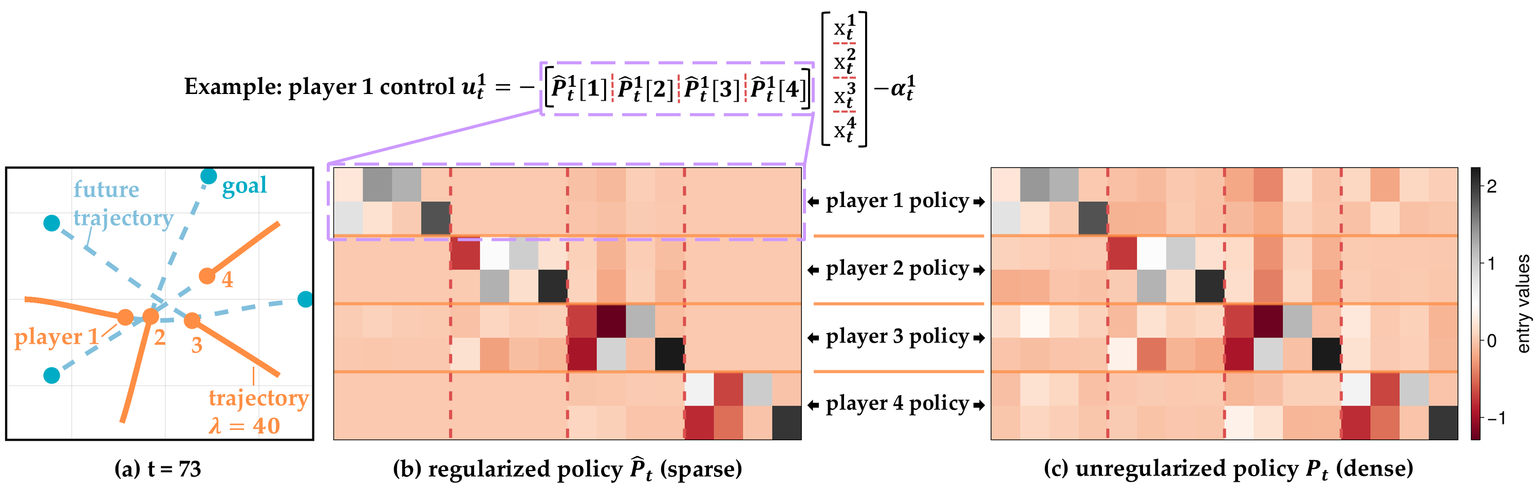
Figure 1. (a) Snapshot of an episode from the navigation game example. (b-c): Regularized and standard Nash equilibrium policy matrices, denoted as $\hat{P}_{t}$ in Eq. 14 and $P_{t}$ in Eq. 13. A policy matrix $P_{t}=[P_{t}^{1\top},\ldots,P_{t}^{N\top}]^{\top}$, aggregated over players, maps all players’ states to joint controls: $u_{t}=-P_{t}x_{t}-\alpha_{t}$. Each policy matrix is divided into $N\times N$ blocks.

(a) Snapshot of an episode from the navigation game example. (b-c): Regularized and standard Nash equilibrium policy matrices, denoted as $\hat{P}_{t}$ in Eq. 14 and $P_{t}$ in Eq. 13. A policy matrix $P_{t}=[P_{t}^{1\top},\ldots,P_{t}^{N\top}]^{\top}$, aggregated over players, maps all players’ states to joint controls: $u_{t}=-P_{t}x_{t}-\alpha_{t}$. Each policy matrix is divided into $N\times N$ blocks, as indicated by the block partition lines above. A sparser policy matrix, characterized by more zero blocks, requires fewer agents’ states to compute control strategies for each agent.

4.2. Non-LQ Dynamic Games

The proposed approach focuses on LQ dynamic games. Nonetheless, our DP-based scheme makes it possible to extend to non-LQ games, i.e., settings where players can have nonquadratic costs and nonlinear dynamics. We employ an iterative algorithm Fridovich-Keil et al. (2020) shown in Algorithm 1 that repeatedly finds LQ approximations of the original dynamic game and solves the approximating LQ games with regularization in Eq. 14 to obtain sparse, approximate feedback Nash equilibrium strategies.

Input: initial state $x_{1}$, game dynamics $\{f_{t}\}_{t\in[T]}$, game costs $\{J^{i}\}_{i\in[N]}$

Initialization: Initial control strategies $\{\hat{\gamma}^{i}\}_{i\in[N]}$

/* Iterative LQ Approximations */

while $\mathrm{not\leavevmode\nobreak\ converged}$ do

       $(x_{1:T+1},u_{1:T})\leftarrow$

       $\qquad\operatorname{ForwardSimulate}(\{\hat{\gamma}^{i}\}_{i\in[N]},x_{1},\{f_{t}\}_{t\in[T]})$

       $(A_{t},B_{t})_{t\in[T]}\leftarrow$

       $\qquad\operatorname{LinearApproximation}(x_{1:T+1},u_{1:T},\{f_{t}\}_{t\in[T]})$

       $(Q^{i}_{t},q^{i}_{t},R^{ij}_{t},r^{ij}_{t})_{i,j\in[N],t\in[T+1]}\leftarrow$

       $\qquad\operatorname{QuadraticApproximation}(x_{1:T+1},u_{1:T},\{J^{i}\}_{i\in[N]})$

       $\{\bar{\hat{\gamma}}^{i}\}_{i\in[N]}\leftarrow$

       $\qquad\operatorname{SolveRegularizedLQGame}(A_{t},B_{t},Q^{i}_{t},q^{i}_{t},R^{ij}_{t},r^{ij}_{t})$

       $\triangleright$ regularization, eq. (14)

       $\{\hat{\gamma}^{i}\}_{i\in[N]}\leftarrow\operatorname{UpdateStrategies}(\{\hat{\gamma}^{i}\}_{i\in[N]},\{\bar{\hat{\gamma}}^{i}\}_{i\in[N]})$

end while

return $\{\hat{\gamma}^{i}\}_{i\in[N]}$

Algorithm 1 Iterative LQ Games with Group Sparsity

5. Results

We extensively evaluate the proposed approach both in non-LQ and LQ dynamic game scenarios to support our key claims made in Section 1.

5.1. Multi-Agent Navigation Game

First, we test the proposed approach in a multi-agent navigation game. This is a non-LQ game and provides an intuitive setting to demonstrate the computed sparsity pattern by our approach over time. We will analyze the performance of the proposed approach more closely in an LQ setting in Section 5.2.

5.1.1. Experiment Setup and Claims

As is shown in Fig. 1 (a), four agents start from the initial positions and drive to their individual goals. All the agents wish to go to their goals as efficiently as possible without too much control efforts while avoiding collision with one another. Hence, they need to compete and find underlying Nash equilibrium strategies. Each agent is modelled using unicycle dynamics with states being 2D position, orientation, and velocity $x_{t}^{i}=[p_{x,t}^{i},p_{y,t}^{i},\phi_{t}^{i},v_{t}^{i}]^{\top}$ and controls being angular and longitudinal acceleration $u_{t}^{i}=[\omega_{t}^{i},a_{t}^{i}]^{\top}$. We provide the definition of players’ running costs in Appendix A.5.

This experiment is designed to support the following claims:

• C1. The proposed approach identifies influential agents and yields more sparse feedback policies than standard Nash equilibrium solutions.

• C2. The algorithm gives different levels of sparsity as the user varies the regularization strength.

• C3. Via an iterative scheme Fridovich-Keil et al. (2020), the proposed approach can be extended to non-LQ dynamic games.

5.1.2. Results

Sparsity Pattern

Figure 1 shows a snapshot of the navigation game and the sparsity pattern in the policy obtained using Algorithm 1. On a high level, as is shown in the heatmaps, the proposed approach computes a more sparse feedback policy in Fig. 1b than the standard Nash equilibrium in Fig. 1c. In this four-player game, a policy matrix $P_{t}$ has 16 blocks corresponding to feedback maps from all players’ states to all players’ controls.

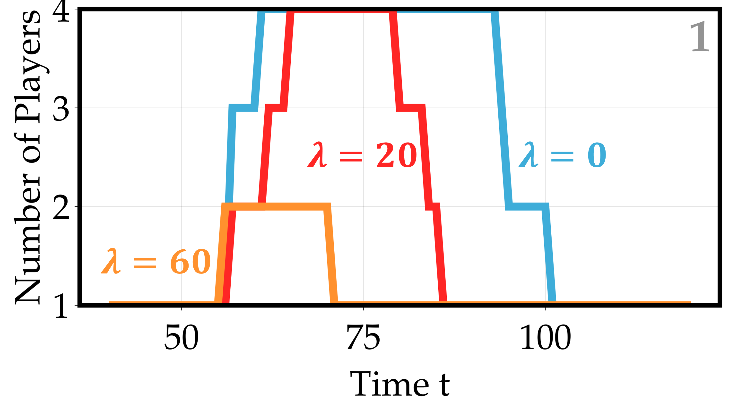
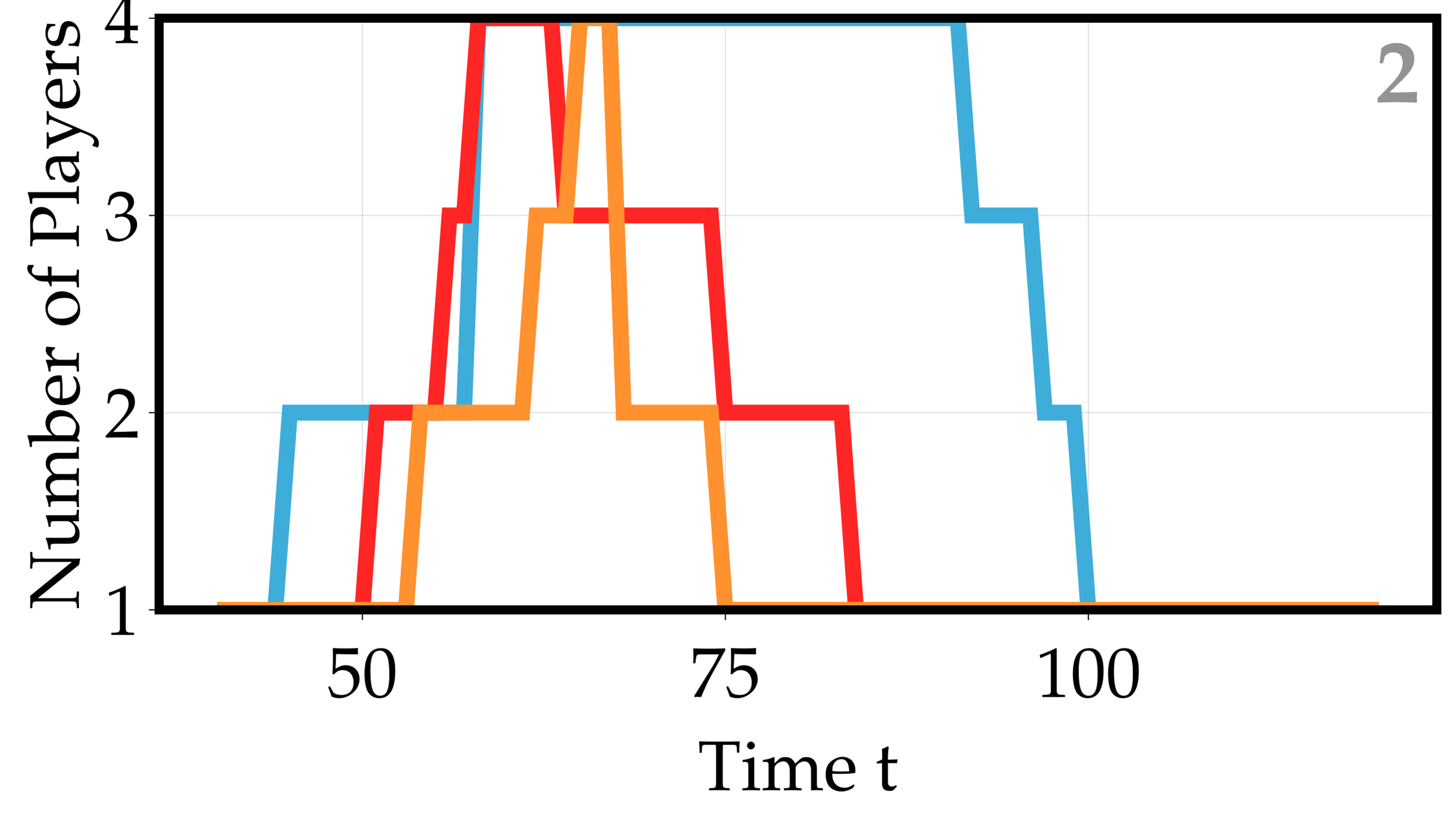
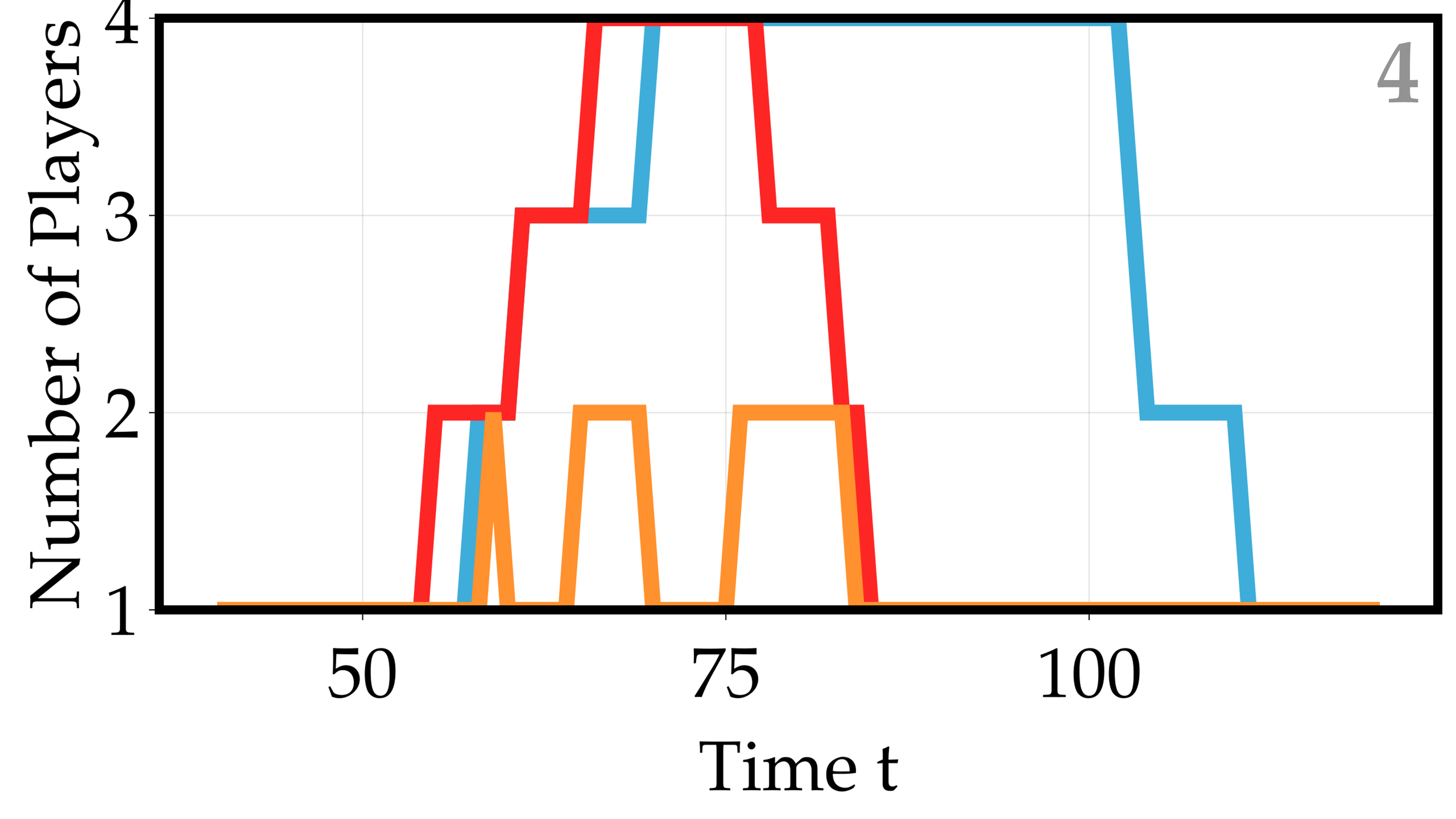
Figure 2. The number of nonzero blocks over time contained in policies of players 1-4 with different regularization levels.

The number of nonzero blocks over time contained in each agent’s policies with different regularization levels.

Figure 3. Snapshot of the proposed approach for an 8-player navigation game and corresponding policy matrices.

Snapshot of the proposed approach for an 8-player navigation game.

At time step $t=73$, because agent $2$ has already passed by agent $1$ and their interaction has been resolved, the regularized policy by our approach chooses to zero out the blocks $(1,2)$ and $(2,1)$ from the policy matrix. Similarly, since agent $4$ is relatively far from agents $1$ and $2$, the regularized policy zeros out the corresponding blocks as well.

Different Regularization Levels

Figure 2 compares the density of the resulting feedback policies from three levels of regularization strength for the same four-player navigation game in Fig. 1. The unregularized Nash equilibrium policy matrix has the highest density in general, as the policy requires state information from the most agents over time. As expected, the proposed approach gives generally more sparse feedback policies with higher regularization strength. Note that this increased sparsity does not appear strictly all the time in Fig. 2. This is because the evaluated non-LQ game is known to have multiple local Nash equilibrium solutions Peters et al. (2020). In the proposed DP approach, each stage’s sparsity depends on sparsity in later stages. Based on the selected regularization level, the proposed approach finds different local solutions where the players pass by one another in different orders.

Scalability

Figure 3 demonstrates our approach for the navigation game with more players, for which encoding sparsity into the computed solution is typically an even more desirable feature.

We note that all the episodes above with different regularization levels result in a collision-free interaction among the agents with only a modest change in players’ costs. We defer a more detailed performance study of our regularization approach to an LQ example in Section 5.2, which has a unique Nash equilibrium solution.

Hence, the results above support the claims C1-3.

5.2. Multi-Robot Formation Game

This section evaluates the proposed approach in an LQ formation game to provide a more detailed performance analysis.

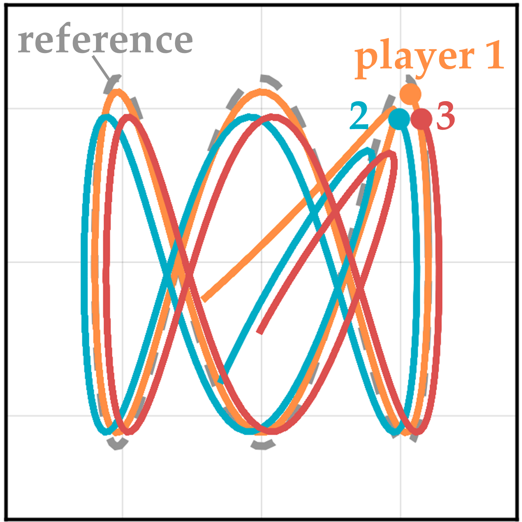
(a)

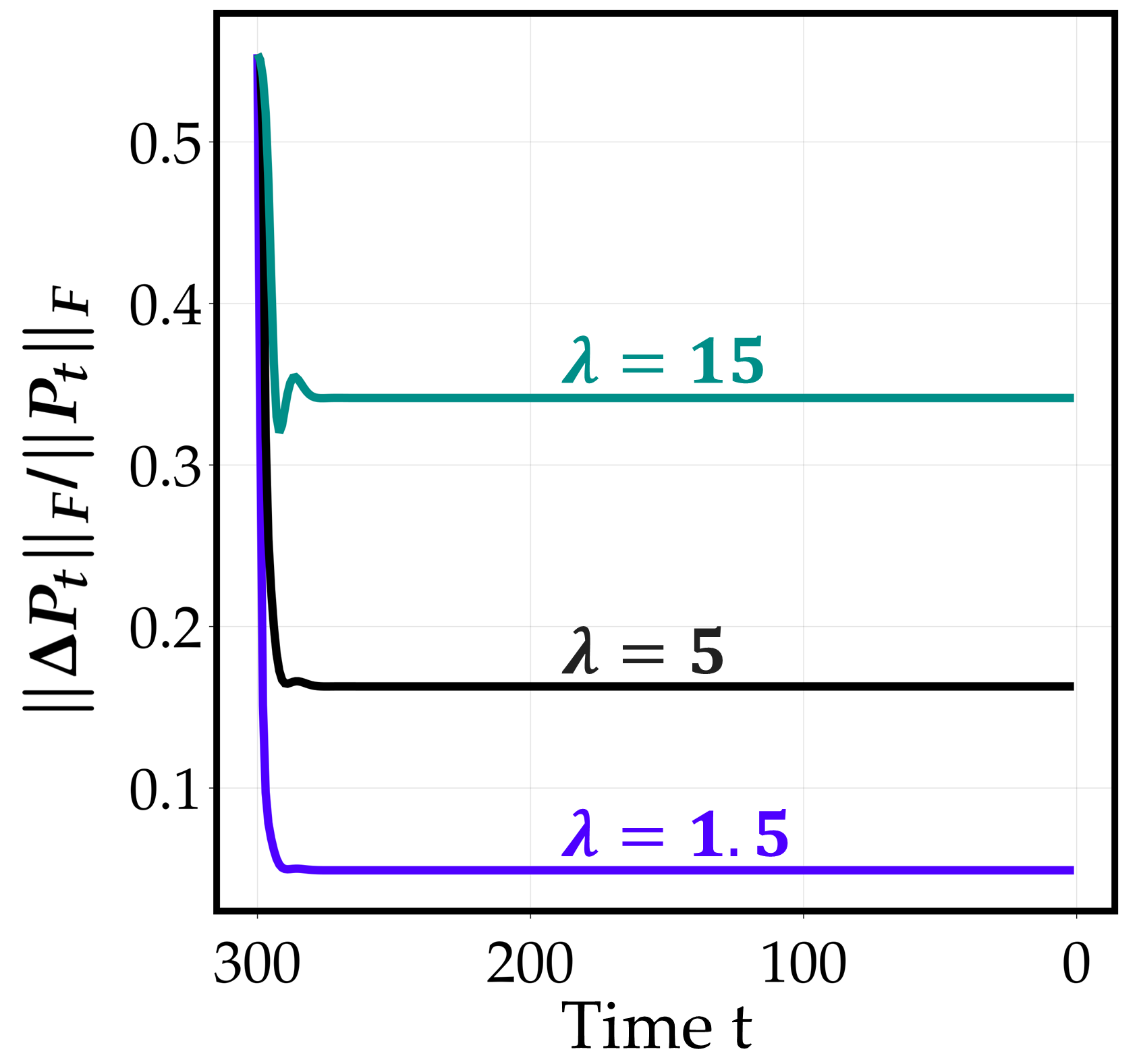
(b)

Figure 4. (a) A three-player formation game: player 1 tracks a reference trajectory shown in grey while players 2 and 3 maintain a formation with respect to player 1. (b) Convergence of regularized policies with different $\lambda$.

(a) A three-player formation game: player 1 tracks a reference trajectory shown in grey while players 2 and 3 maintain a formation with respect to player 1. (b) Convergence of regularized policies with different $\lambda$.

5.2.1. Experiment Setup and Claims

Figure 4(a) shows the following scenario: player 1 tracks a predefined sinusoidal trajectory, while player 2 is tasked to maintain a relative position with players 1 and 3, and likewise for player 3. Hence, player 1’s cost is independent of the other players, while costs for players 2 and 3 are defined by other players’ positions. As a result, the players need to maintain a formation together while tracking the sinusoidal trajectory. Each player’s dynamics are modelled as a planar double integrator with states being position and velocity $x_{t}^{i}=[p_{x,t}^{i},v_{x,t}^{i},p_{y,t}^{i},v_{y,t}^{i}]^{\top}$ and controls being acceleration $u_{t}^{i}=[a_{x,t}^{i},a_{y,t}^{i}]$. We provide the definition of players’ costs in Appendix A.5.

This experiment is designed to support the following claim:

• C4. For all interacting agents whose costs are coupled with other agents’ states, the sparse strategies computed by our approach improve robustness and task performance over standard Nash equilibrium solutions when agents only have inaccurate (e.g., noisy) estimates of other agents’ states.

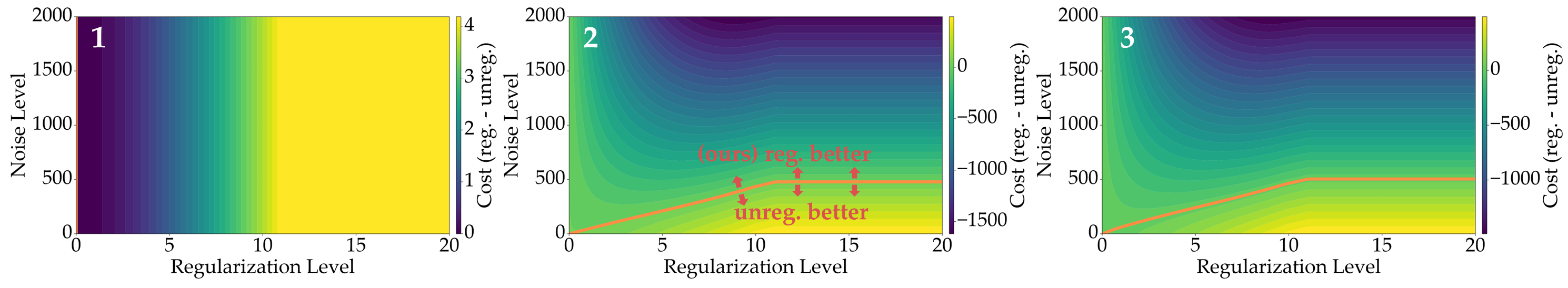
Figure 5. Costs of players 1-3 subtracted by standard Nash equilibrium costs in a formation game, averaged over 100 random initial players’ positions, for varying noise and regularization levels. In subplots 2-3, the orange lines indicate the zero level set.

Players’ costs subtracted by standard Nash equilibrium costs for various noise and regularization levels in a formation game. Orange lines in subplots (1,2) and (1,3) denote zero level set.

Figure 6. Formation game trajectories under noise level 520 with different regularization levels; left to right: $\lambda=0,1.5,5\leavevmode\nobreak\ (\text{optimal}),15$.

Trajectories under noise level 520 with different regularization levels; left to right: $\lambda=0.0,1.5,5.0,15.0$.

5.2.2. Results

Figure 4(a) illustrates a resulting trajectory generated by a standard Nash equilibrium strategy, serving as the ground truth behavior. The three players follow the task trajectory from their initial positions, forming a triangular formation along the path. Figure 4(b) shows the convergence of the policy deviation, $\Delta P_{t}$, across DP iterations for various $\lambda$ values. Notably, the regularized DP recursion converges even for a high $\lambda=15$, which completely zeros out the off-diagonal blocks of the policy matrices. This convergence validates the theoretical results of Theorems 5 and 6.

Monte Carlo Study

To better understand our regularized strategies’ performance, especially when other agents’ state information might be inaccurate, we evaluate the proposed approach in scenarios where players only have access to noisy state estimates of other players. Players make decisions separately with perfect state information about themselves and noisy state information about other players. We run a Monte Carlo study under zero-mean isotropic Gaussian noise with 50 different variance levels starting from zero. We compare standard Nash equilibrium strategies against the regularized strategies by our approach with 100 different regularization levels. For each combination of a noise and a regularization level, we run both approaches starting from 100 random players’ positions uniformly sampled from a square measured 20 meters $\times$ 20 meters and centred at the origin. Hence, the experiment includes $5\times 10^{5}$ comparisons in total.

Figure 5 shows the cost performance of the regularized strategies subtracted by standard Nash equilibrium costs and averaged over 100 random players’ initial positions, where a negative value indicates that the proposed approach yields better performance in this setting.

Recall that player 1’s cost is not coupled with the other players and we only regularize the off-diagonal blocks in the policy matrices, corresponding to inter-agent dependencies. As shown in Fig. 5, player 1’s performance is invariant with different noise levels and almost invariant with different regularization levels. The cost of player 1 has a tiny increase with higher regularization. This is because the block $(1,1)$ of the policy matrices is slightly biased by the regularization applied to neighborhood blocks, which we shall explain in detail in Appendix A.6. Nonetheless, the cost change is only up to 0.35%.

Players 2 and 3 show the same trend in their performance with different noise and regularization levels. In columns 2 and 3 of Fig. 5, the parts above the orange zero level set line indicate trials where the proposed approach performs better. On a high level, the regularized strategies computed by the proposed approach outperform the standard Nash equilibrium strategies for the majority of the trials (around 82%). An important observation is: For any positive (even if small) noise level, there exists an interval of regularization levels where the sparse policies perform better than the standard Nash equilibrium policies; the optimal regularization level is always strictly positive for any nonzero noise level. As the noise level increases, the interval where the regularized policies perform better also grows. Above noise level around 500, any regularized policies computed by the proposed approach yield lower costs than the standard Nash equilibrium.

Therefore, the results above validate the claim C4.

Qualitative Results

Figure 6 shows the resulting trajectories from standard Nash equilibrium strategies compared with the proposed approach with different regularization levels. Under noise-corrupted state estimates, standard Nash equilibrium strategies greedily optimize players 2 and 3’s costs and yield noisy, high-cost trajectories. By contrast, with higher regularization, the proposed approach regularizes the solutions more and forces the strategies to be less dependent on other players’ states. As a result, players 2 and 3 move in smaller sinusoidal shapes and their motion becomes less sensitive to other players’ noisy states. In the extreme high-regularization case $\lambda=15$, players 2 and 3’s strategies become completely independent of other players and yield smooth sinusoidal trajectories. Among the regularization levels, $\lambda=5$ gives the lowest costs for players 2 and 3 in this setting.

6. Conclusion

We have presented a regularized DP approach for finding sparse feedback policies in noncooperative games. The regularized policies selectively depend on a subset of agents’ states, thereby reducing the communication and sensing resources required for execution. The proposed approach encodes structured sparsity into LQ game solutions via solving a convex adaptive group Lasso problem at each DP iteration. This approach is further extended to general non-LQ games via iterative LQ approximations.

For LQ games, we establish an upper bound on the single-stage difference between the regularized and standard Nash equilibrium policy matrices. Thus equipped, we prove the asymptotic convergence of the regularized solution to a neighborhood of the Nash equilibrium across all game stages.

Extensive results in multi-robot navigation tasks validate the efficacy of the proposed approach in producing sparse feedback policies at varying regularization levels and demonstrate its scalability to games involving multiple players. Monte Carlo studies in a multi-agent formation game also show that when interacting agents with coupled costs have noisy observations of other agents’ states, it is always better to employ some (nonzero) degree of regularization. In this case, the regularized policies consistently outperform standard Nash equilibrium solutions by selectively ignoring information that may be inaccurate.

Future work could explore the optimal selection of regularization strengths across different game stages. Additionally, applying the proposed regularization scheme to scenarios involving more complex uncertainties beyond observation noise is also an interesting direction. Lastly, a deeper investigation into the observation presented in Section 5.1—where our approach yields distinct local solutions at different regularization levels—would be of interest.

We thank Yue Yu for his helpful discussions about convergence analysis. This work was supported in part by the Office of Naval Research (ONR) under Grants ONR N00014-24-1-2797 and ONR N00014-22-1-2703, and in part by the National Science Foundation (NSF) under Grant No. 2409535, and in part by the Army Research Laboratory and was accomplished under Cooperative Agreement Number W911NF-23-2-0011.

Appendix A Appendix

A.1. Proof of Lemma 4

Proof.

We rewrite the unregularized system of equations in Eq. 13 as an optimization problem:

$$\min_{P_{t}}\underbrace{\frac{1}{2}\|S_{t}P_{t}-Y_{t}\|_{F}^{2}}_{h(P_{t})},$$ (20)

and we have the regularized problem in Eq. 14:

$$\min_{\hat{P}_{t}}\hat{h}(\hat{P}_{t})=\underbrace{\frac{1}{2}\|S_{t}\hat{P}_{t}-Y_{t}\|_{F}^{2}}_{h(\hat{P}_{t})}+\underbrace{\sum_{i,j}\lambda_{i,j}\|\hat{P}_{t}^{i}[j]\|_{F}}_{\psi(\hat{P}_{t})},$$ (21)

where $\hat{P}_{t}^{i}[j]\in\mathbb{R}^{n^{i}\times m^{j}}$ denotes the $(i,j)$ block of the $\hat{P}_{t}$ matrix. We recall the dimensions of players’ states and controls $x_{t}^{i}\in\mathbb{R}^{m^{i}},u_{t}^{i}\in\mathbb{R}^{n^{i}}$, and $m=\sum_{i\in[N]}m^{i}$, $n=\sum_{i\in[N]}n^{i}$. Hence, we have $S_{t}\in\mathbb{R}^{n\times n}$, and $P_{t},\hat{P}_{t}\in\mathbb{R}^{n\times m}$.

First, we examine the optimality conditions for both problems and characterize their solutions. Then, we bound the difference between the two solutions.

Optimality conditions.

The unregularized problem in Eq. 20 is a convex optimization problem with a differentiable objective function, whose necessary and sufficient optimality condition (Boyd and Vandenberghe, 2004, Ch.4) is:

$$\nabla_{P_{t}}h(P_{t})=0\Rightarrow M_{t}P_{t}-S_{t}^{\top}Y_{t}=0\Rightarrow P_{t}=M_{t}^{-1}S_{t}^{\top}Y_{t},$$ (22)

where we define $M_{t}=S_{t}^{\top}S_{t}$ and recall that $S_{t}$ is full rank by 1.

The objective of the regularized problem in Eq. 21 is nonsmooth but convex. Since $h$ is convex and differentiable and $\psi$ is convex and finite-valued, we have the necessary and sufficient optimality condition (Recht and Wright, 2019, Thm 8.17):

$$0\in\nabla_{\hat{P}_{t}}h(\hat{P}_{t})+\partial_{\hat{P}_{t}}\psi(\hat{P}_{t})\\ =M_{t}\hat{P}_{t}-S_{t}^{\top}Y_{t}+\partial_{\hat{P}_{t}}(\sum_{i,j}\lambda_{i,j}\|\hat{P}_{t}^{i}[j]\|_{F}),$$

where $\partial(\cdot)$ denotes the subdifferential set. Since $\psi$ is convex and finite-valued (Recht and Wright, 2019, Thm 8.11), we have:

$$\partial_{\hat{P}_{t}}\psi=\partial_{\hat{P}_{t}}(\sum_{i,j}\lambda_{i,j}\|\hat{P}_{t}^{i}[j]\|_{F})=\sum_{i,j}\lambda_{i,j}\partial_{\hat{P}_{t}}(\|\hat{P}_{t}^{i}[j]\|_{F}).$$

Therefore, we obtain the optimality condition:

$$0\in M_{t}\hat{P}_{t}-S_{t}^{\top}Y_{t}+\sum_{i,j}\lambda_{i,j}\partial_{\hat{P}_{t}}(\|\hat{P}_{t}^{i}[j]\|_{F}).$$ (23)

The subdifferential for $\|\hat{P}_{t}^{i}[j]\|_{F}$ is given by:

$$\partial_{\hat{P}_{t}^{i}[j]}(\|\hat{P}_{t}^{i}[j]\|_{F})=\begin{cases}\frac{\hat{P}_{t}^{i}[j]}{\|\hat{P}_{t}^{i}[j]\|_{F}},\hat{P}_{t}^{i}[j]\neq 0\\ \{z\mid z\in\mathbb{R}^{n^{i}\times m^{j}},\|z\|_{F}\leq 1\},\hat{P}_{t}^{i}[j]=0.\par\end{cases}$$ (24)

Therefore, elements in the subdifferential $\partial_{\hat{P}_{t}}(\|\hat{P}_{t}^{i}[j]\|_{F})$ are matrices that have entries shown in Eq. 24 for block $(i,j)$ and zeros elsewhere.

For a solution $\hat{P}_{t}$ that satisfies the optimality condition in Eq. 23, we must be able to find a particular set of subgradients $\theta^{*}_{1,1}$, $\theta^{*}_{1,2}$, $\ldots$, $\theta^{*}_{N,N}$ from the subdifferential sets such that:

$$0=M_{t}\hat{P}_{t}-S_{t}^{\top}Y_{t}+\sum_{i,j}\lambda_{i,j}\theta_{i,j}^{*},$$

where $\theta^{*}_{i,j}\in\mathbb{R}^{n\times m},\theta^{*}_{i,j}\in\partial_{\hat{P}_{t}}(\|\hat{P}_{t}^{i}[j]\|_{F})$. Such a point specifies a solution for the regularized problem, i.e.

$$\hat{P}_{t}=M_{t}^{-1}S_{t}^{\top}Y_{t}-\sum_{i,j}\lambda_{i,j}M_{t}^{-1}\theta_{i,j}^{*}.$$ (25)

Bounding the solution difference.

Having characterized solutions to the two problems in Eqs. 20 and 21, we summarize Eq. 22 and Eq. 25 to compute the difference between the solutions:

$$\|\Delta P_{t}\|_{F}=\|\hat{P}_{t}-P_{t}\|_{F}=\|\sum_{i,j}\lambda_{i,j}M_{t}^{-1}\theta_{i,j}^{*}\|_{F}\\ \leq\sum_{i,j}\lambda_{i,j}\|M_{t}^{-1}\theta_{i,j}^{*}\|_{F}.$$ (26)

Next, we split the terms in $\sum_{i,j}\lambda_{i,j}\|M_{t}^{-1}\theta_{i,j}^{*}\|_{F}$ into two cases based on Eq. 24.

Case 1. For blocks $(i,j)$ such that $\hat{P}_{t}^{i}[j]\neq 0$, we have that $\|\theta^{*}_{i,j}\|_{F}=1$. We denote a vectorization operator as $\mathrm{vec(\cdot)}$. We note that we can rewrite the multiplication $M_{t}^{-1}\theta_{i,j}^{*}$ in a matrix-vector form such that $\|\tilde{M_{t}}^{-1}\tilde{\theta}^{*}_{i,j}\|_{2}=\|M_{t}^{-1}\theta_{i,j}^{*}\|_{F}$, where the matrix $\tilde{M_{t}}^{-1}:=\mathrm{blogdiag}(M_{t}^{-1},\ldots,M_{t}^{-1})\in\mathbb{R}^{mn\times mn}$ is the block diagonal concatenation of $m$ copies of $M_{t}^{-1}$, and $\tilde{\theta}^{*}_{i,j}:=\mathrm{vec}{(\theta^{*}_{i,j})}\in\mathbb{R}^{mn}$.

From the definition of the matrix spectral norm, we have:

$$\|\tilde{M_{t}}^{-1}\|_{2}=\sup_{\|\tilde{\theta}^{*}_{i,j}\|_{2}=1}\|\tilde{M_{t}}^{-1}\tilde{\theta}^{*}_{i,j}\|_{2}$$ (27)

Hence,

$$\lambda_{i,j}\|M_{t}^{-1}\theta^{*}_{i,j}\|_{F} =\lambda_{i,j}\|\tilde{M_{t}}^{-1}\tilde{\theta}^{*}_{i,j}\|_{2}$$ (28)

$$\leq\lambda_{i,j}\|\tilde{M_{t}}^{-1}\|_{2}=\lambda_{i,j}\sigma_{\mathrm{max}}(\tilde{M_{t}}^{-1}),$$

where $\sigma$ denotes singular values. We note that, since $\tilde{M_{t}}$ has a block-diagonal structure, it is straightforward to verify that $\sigma_{\mathrm{max}}(\tilde{M_{t}}^{-1})=\sigma_{\mathrm{max}}(M_{t}^{-1})$.

Case 2. For blocks $(i,j)$ such that $\hat{P}_{t}^{i}[j]=0$, since we know $\|\tilde{\theta}^{*}_{i,j}\|_{2}\leq 1$, we have:

$$\|M_{t}^{-1}\theta^{*}_{i,j}\|_{F}=\|\tilde{M_{t}}^{-1}\tilde{\theta}^{*}_{i,j}\|_{2} \leq\sup_{\|\tilde{\theta}^{*}_{i,j}\|_{2}\leq 1}\|\tilde{M_{t}}^{-1}\tilde{\theta}^{*}_{i,j}\|_{2}$$ (29)

$$\leq\sup_{\|\tilde{\theta}^{*}_{i,j}\|_{2}=1}\|\tilde{M_{t}}^{-1}\tilde{\theta}^{*}_{i,j}\|_{2}$$

$$=\|\tilde{M_{t}}^{-1}\|_{2}$$

$$=\sigma_{\mathrm{max}}(\tilde{M_{t}}^{-1})$$

$$=\sigma_{\mathrm{max}}(M_{t}^{-1}).$$

Recall that we require the original system of equations in Eq. 13 to have a unique solution, i.e., $S_{t}$ has full rank. Therefore, $M_{t}$ has positive singular values and it follows that $\sigma_{\mathrm{max}}(M_{t}^{-1})=\frac{1}{\sigma_{\mathrm{min}}(M_{t})}=\frac{1}{\sigma_{\mathrm{min}}^{2}(S_{t})}$. Hence, summarizing the two cases,

$$\|\Delta P_{t}\|_{F}\leq\frac{\sum_{i,j\in[N]}\lambda_{i,j}}{\sigma_{\mathrm{min}}^{2}(S_{t})}$$ (30)

bounds the difference between the regularized and unregularized solutions at a single time step $t$. ∎

A.2. Proof of Theorem 5

A.2.1. Definition of the Dynamical System

This section defines the dynamical system $\hat{\tilde{Z}}_{t}=\tau(\hat{\tilde{Z}}_{t+1},\delta_{t})$ studied in Theorem 5.

For all $i\in[N]$, we have algebraic coupled Riccati equations in Eq. 16 for infinite-horizon LQ game:

$$Z^{i*}=Q^{i}+\sum_{j=1}^{N}P^{j*\top}R^{ij}P^{j*}+F^{*\top}Z^{i*}F^{*}.$$ (31)

For finite-horizon LQ games, we have unregularized coupled Riccati recursion LABEL:eq:value-func:

$$Z_{t}^{i}=Q^{i}+\sum_{j=1}^{N}P_{t}^{j\top}R^{ij}P_{t}^{j}+F_{t}^{\top}Z^{i}_{t+1}F_{t},$$ (32)

and regularized coupled Riccati recursion in Eq. 15:

$$\hat{Z}_{t}^{i}=Q^{i}+\sum_{j=1}^{N}\hat{P}_{t}^{j\top}R^{ij}\hat{P}_{t}^{j}+\hat{F}_{t}^{\top}\hat{Z}^{i}_{t+1}\hat{F}_{t},$$ (33)

where:

$$\hat{P}_{t}^{j}=P^{j}_{t}+\Delta P^{j}_{t},\quad\hat{F}_{t}=F_{t}-\sum_{j=1}^{N}B^{j}\Delta P^{j}_{t}.$$

In order to study the convergence of the regularized coupled Riccati recursion, we analyze the asymptotic difference between Eq. 33 and Eq. 31, for all $i\in[N]$:

$$\hat{\tilde{Z}}^{i}_{t} :=\hat{Z}_{t}^{i}-Z^{i*}$$

$$=\sum_{j=1}^{N}\hat{P}_{t}^{j\top}R^{ij}\hat{P}_{t}^{j}+\hat{F}_{t}^{\top}\hat{Z}^{i}_{t+1}\hat{F}_{t}-\sum_{j=1}^{N}P^{j*\top}R^{ij}P^{j*}-F^{*\top}Z^{i*}F^{*}$$

$$=\sum_{j=1}^{N}(P_{t}^{j}+\Delta P_{t}^{j})^{\top}R^{ij}(P_{t}^{j}+\Delta P_{t}^{j})+(F_{t}-\sum_{j=1}^{N}B^{j}\Delta P_{t}^{j})^{\top}\hat{Z}_{t+1}^{i}$$

$$\quad\cdot(F_{t}-\sum_{k=1}^{N}B^{k}\Delta P_{t}^{k})-\sum_{j=1}^{N}P^{j*\top}R^{ij}P^{j*}-F^{*\top}Z^{i*}F^{*}$$

$$=\underbrace{{\color[rgb]{0,0,1}\sum_{j=1}^{N}P_{t}^{j^{\top}}R^{ij}P_{t}^{j}+F_{t}^{\top}\hat{Z}_{t+1}^{i}F_{t}-\sum_{j=1}^{N}P^{j*\top}R^{ij}P^{j*}-F^{*\top}Z^{i*}F^{*}}}_{{\color[rgb]{0,0,1}\phi^{i}(\hat{Z}_{t+1})}}$$ (34)

$${\color[rgb]{1,0,0}\quad+\sum_{j=1}^{N}\Delta P_{t}^{j\top}R^{ij}P_{t}^{j}+\sum_{j=1}^{N}\Delta P_{t}^{j\top}R^{ij}\Delta P_{t}^{j}+\sum_{j=1}^{N}P_{t}^{j\top}R^{ij}\Delta P_{t}^{j}}$$

$${\color[rgb]{1,0,0}\quad-\sum_{j=1}^{N}\Delta P_{t}^{j\top}B^{j\top}\hat{Z}_{t+1}^{i}F_{t}-F_{t}^{\top}\hat{Z}_{t+1}^{i}\sum_{k=1}^{N}B^{k}\Delta P_{t}^{k}}$$

$${\color[rgb]{1,0,0}\quad+\sum_{j=1}^{N}\Delta P_{t}^{j\top}B^{j\top}\hat{Z}_{t+1}^{i}\sum_{k=1}^{N}B^{k}\Delta P_{t}^{k}}$$

$$={\color[rgb]{0,0,1}\phi^{i}(\hat{Z}_{t+1})}+{\color[rgb]{1,0,0}O^{i}(\hat{Z}_{t+1},\Delta P_{t})}.$$

Hence:

$$\hat{\tilde{Z}}^{i}_{t}=\hat{Z}_{t}^{i}-Z^{i*}={\color[rgb]{0,0,1}\phi^{i}(\hat{Z}_{t+1})}+{\color[rgb]{1,0,0}O^{i}(\hat{Z}_{t+1},\Delta P_{t})}.$$ (35)

Aggregating all the players $\hat{\tilde{Z}}_{t}:=[\hat{\tilde{Z}}^{1\top}_{t},\dots,\hat{\tilde{Z}}^{N\top}_{t}]^{\top}$, we have:

$$\hat{\tilde{Z}}_{t}=\hat{Z}_{t}-Z^{*}={\color[rgb]{0,0,1}\phi(\hat{Z}_{t+1})}+{\color[rgb]{1,0,0}O(\hat{Z}_{t+1},\Delta P_{t})}.$$ (36)

We define the dynamical system in Eq. 36 as:

$$\hat{\tilde{Z}}_{t}=\tau(\hat{\tilde{Z}}_{t+1},\delta_{t}),$$ (37)

where we denote regularization difference $\Delta P_{t}$ as disturbance $\delta_{t}$. The system in Eq. 37 is the dynamical system we referred to in Theorem 5.

A.2.2. Proof of Theorem 5

Proof.

In Eq. 37, the system dynamics $\tau(\hat{\tilde{Z}}_{t+1},\delta_{t})$ consist of the nominal part ${\color[rgb]{0,0,1}\phi(\hat{Z}_{t+1})}$ and the part which directly depends upon disturbances ${\color[rgb]{1,0,0}O(\hat{Z}_{t+1},\Delta P_{t})}$, as expanded in Eq. 34. When there is no regularization, i.e., $\Delta P_{t}=0$ and $\hat{Z}_{t}=Z_{t},\forall t$, we have ${\color[rgb]{1,0,0}O(\hat{Z}_{t+1},\Delta P_{t})}=0$ and the system $\hat{\tilde{Z}}_{t}=\tau(\hat{\tilde{Z}}_{t+1},\delta_{t})$ reduces to $\tilde{Z}_{t}=\tau(\tilde{Z}_{t+1},0)$, which only has the nominal part and is exactly the difference between Eq. 32 and Eq. 31 aggregated over all the players. That is, at zero regularization, the dynamical system in Eq. 37 reduces to the difference between the unregularized finite-horizon Riccati and infinite-horizon Riccati equations.

By 2, the dynamical system in Eq. 37 with zero regularization $\tilde{Z}_{t}=\tau(\tilde{Z}_{t+1},0)={\color[rgb]{0,0,1}\phi(Z_{t+1})}$ is locally asymptotically stable at the origin. Furthermore, the system in Eq. 37 is continuous in both value matrix $\hat{Z}_{t+1}$ and disturbance $\Delta P_{t}$, and therefore in $\hat{\tilde{Z}}_{t+1}$ and $\delta_{t}$. Hence, the system in Eq. 37 is locally ISS with respect to the regularization (Jiang et al., 2004, Lemma 2.2).

We recall the definitions of class $\mathcal{K}$ and class $\mathcal{KL}$ functions Khalil (2002):

Definition 0.

A continuous function $\rho:\mathbb{R}_{\geq 0}\rightarrow\mathbb{R}_{\geq 0}$ belongs to class $\mathcal{K}$ if it is strictly increasing with $\rho(0)=0$. A continuous function $\beta:\mathbb{R}_{\geq 0}\times\mathbb{R}_{\geq 0}\rightarrow\mathbb{R}_{\geq 0}$ belongs to class $\mathcal{KL}$ if $\beta(\cdot,k)$ is of class $\mathcal{K}$ for each fixed $k$, and $\beta(r,\cdot)$ is decreasing for each fixed $r$, and $\lim_{k\rightarrow\infty}\beta(r,k)=0$.

From the definition of local input-to-state stability (Jiang et al., 2004, Definition 2.1), there exist a class $\mathcal{KL}$ function $\beta$ and a class $\mathcal{K}$ function $\rho$ such that:

$$\|\hat{\tilde{Z}}_{t}\|_{F}\leq\beta(\|\hat{\tilde{Z}}_{T+1}\|_{F},T-t)+\rho(\|\delta_{t}\|_{\infty}),\forall t\in(-\infty,T],$$ (38)

for disturbances such that $\sup_{t\leq\tau\leq T}\|\delta_{\tau}\|_{F}=\|\delta_{t}\|_{\infty}<\delta,\delta\in\mathbb{R}_{>0}$, and $\|\hat{\tilde{Z}}_{T+1}\|_{F}\leq z,z\in\mathbb{R}_{>0}$. ∎

A.3. Proof of Corollary 6

Proof.

In Eq. 38, since $\beta(\|\hat{\tilde{Z}}_{T+1}\|_{F},T-t)$ decays to 0 as $t\rightarrow-\infty$, for every $\epsilon>0$ there exists $t^{\star}\in(-\infty,T]$ such that if $t\in(-\infty,t^{\star}]$ then

$$\|\hat{\tilde{Z}}_{t}\|_{F}\leq\frac{\epsilon}{2}+\rho(\|\delta_{t}\|_{\infty}),\leavevmode\nobreak\ \forall t\in(-\infty,t^{\star}].$$ (39)

In addition, because $\rho(\|\delta_{t}\|_{\infty})$ is class $\mathcal{K}$, for an arbitrary ball with radius $\epsilon>0$, there exists a positive constant $\xi_{1}>0$ such that the following relation holds:

$$\|\delta_{t}\|_{\infty}\leq\xi_{1}\implies\rho(\|\delta_{t}\|_{\infty})\leq\frac{\epsilon}{2}.$$ (40)

Therefore, combining Eq. 39 and Eq. 40 and given that the conditions in Theorem 5 hold, for every $\epsilon>0$ there exists $t^{\star}\in(-\infty,T]$ and $\xi_{1}>0$ such that if $\|\delta_{t}\|_{\infty}\leq\xi_{1}$ then

$$\|\hat{\tilde{Z}}_{t}\|_{F}\leq\epsilon,\leavevmode\nobreak\ t\in(-\infty,t^{\star}].$$ (41)

That is, for small disturbances $\delta_{t}$, $\hat{\tilde{Z}}_{t}$ will eventually enter and stay inside the ball of radius $\epsilon$.

Eq. 41 is true given a condition on $\|\delta_{t}\|_{\infty}$, which we now need to relate to the regularization constants $\lambda_{i,j}$. To that end, recall that the regularized $\hat{S}_{t}$ takes the form:

$$\begin{aligned} \hat{S}_{t}=\begin{bmatrix}R^{11}+B^{1\top}\hat{Z}_{t+1}^{1}B^{1}&.&\ldots&B^{1\top}\hat{Z}_{t+1}^{1}B^{N}\\ B^{2\top}\hat{Z}_{t+1}^{2}B^{1}&.&\ldots&B^{2\top}\hat{Z}_{t+1}^{2}B^{N}\\ \vdots&\dot{\hfil}&\ddots&\vdots\\ B^{N\top}\hat{Z}_{t+1}^{N}B^{1}&.&\ldots&R^{NN}+B^{N\top}\hat{Z}_{t+1}^{N}B^{N}\\ \end{bmatrix}.\end{aligned}$$ (42)

For infinite-horizon LQ games, taking the limit $t\rightarrow-\infty$, we have the infinite-horizon counterpart of $S_{t}$ as follows:

$$\begin{aligned} S^{*}=\begin{bmatrix}R^{11}+B^{1\top}Z^{1*}B^{1}&.&\ldots&B^{1\top}Z^{1*}B^{N}\\ B^{2\top}Z^{2*}B^{1}&.&\ldots&B^{2\top}Z^{2*}B^{N}\\ \vdots&\dot{\hfil}&\ddots&\vdots\\ B^{N\top}Z^{N*}B^{1}&.&\ldots&R^{NN}+B^{N\top}Z^{N*}B^{N}\\ \end{bmatrix}.\end{aligned}$$ (43)

By 1, the unregularized $S_{t}$ in Eq. 13 and $S^{*}$ in Eq. 43 are of full rank. Therefore, $\inf_{t}\sigma_{\mathrm{min}}(S_{t})=v>0$. In addition, we observe that when $\sum_{i,j\in[N]}\lambda_{i,j}\rightarrow 0$, we have $\hat{S}_{t}\rightarrow S_{t}$ and $\hat{Z}_{t}\rightarrow Z_{t}$ pointwise in $t$. By the continuity of the singular values, this implies that for every $t^{\star}\in(-\infty,T]$ there exists $\xi_{2}>0$ such that if $\sum_{i,j\in[N]}\lambda_{i,j}\leq\xi_{2}$ then $\sigma_{\mathrm{min}}(\hat{S}_{t})\geq v/2$ for all $t\in[t^{\star},T]$. In addition, it implies that $\|\hat{\tilde{Z}}_{t^{\star}}\|_{F}\leq\epsilon$ if $t^{\star}$ is chosen to be sufficiently small, because $Z_{t}\rightarrow Z^{*}$ as $t\rightarrow-\infty$. In other words, for small disturbances, $\sigma_{\mathrm{min}}(\hat{S}_{t})$ will remain uniformly away from zero for a given amount $t\in[t^{\star},T]$, and $\hat{Z}_{t}$ will enter a ball of radius $\epsilon$ around $Z^{*}$ at $t^{\star}$. It then remains to show that $\hat{Z}_{t}$ will also stay in that ball for all $t\leq t^{\star}$.

Given that $\|\hat{\tilde{Z}}_{t^{\star}}\|_{F}\leq\epsilon$, we can subsequently prove that $\|\hat{\tilde{Z}}_{t}\|_{F}\leq\epsilon$ for all $t\in(-\infty,t^{\star}]$ by induction. In particular, from Lemma 4, if we require

$$\frac{\sum_{i,j\in[N]}\lambda_{i,j}}{(\frac{\nu}{2})^{2}}\leq\xi_{1},$$ (44)

then we guarantee $\eqref{eq:condition-disturbance}$ holds at time $t=t^{\star}$, and thus $\|\hat{\tilde{Z}}_{t^{\star}-1}\|_{F}\leq\epsilon$ from Eq. 39. Choosing $\epsilon>0$ small enough so that $\sigma_{\mathrm{min}}(\hat{S}_{t})\geq v/2$ for any $\|\hat{\tilde{Z}}_{t}\|_{F}\leq\epsilon$, it follows that $\sigma_{\mathrm{min}}(\hat{S}_{t^{\star}-1})\geq v/2$, hence also $\|\hat{\tilde{Z}}_{t^{\star}-2}\|_{F}\leq\epsilon$ by Eq. 44 and Lemma 4. We can follow this argument recursively and show that $\|\hat{\tilde{Z}}_{t}\|_{F}\leq\epsilon$ for all $t\in(-\infty,t^{\star}]$, and thus

$$\limsup_{t\rightarrow-\infty}\|\hat{\tilde{Z}}_{t}\|_{F}\leq\epsilon.$$ (45)

To conclude, recall that the above results hold if we choose $\xi$ in Corollary 6 to be $\xi=\mathrm{min}((\frac{\nu}{2})^{2}\xi_{1},\xi_{2})$.

∎

A.4. Transformation of Group Lasso Problem to a Conic Program

The group Lasso problem in Eq. 14 can be reformulated as a conic program, as described below. Observe that Eq. 14 can be rewritten as:

$$\min_{\hat{P}_{t}} \frac{1}{2}\|(I_{N}\otimes S_{t})\textrm{vec}(\hat{P}_{t})-\textrm{vec}(Y_{t})\|_{2}^{2}+\sum_{i,j}\lambda_{i,j}\|\textrm{vec}(\hat{P}_{t}^{i}[j])\|_{2},$$ (46)

where $\otimes$ is the Kronecker product. Let ${s_{i,j}\in\mathbb{R}}$ be a slack variable. We define $s:=\{s_{i,j},\forall i,j\in[N]\}$. By using the epigraph trick Boyd and Vandenberghe (2004), we can rewrite (46) as a conic program with quadratic cost:

$$\min_{\hat{P}_{t},s} \frac{1}{2}\|(I_{N}\otimes S_{t})\textrm{vec}(\hat{P}_{t})-\textrm{vec}(Y_{t})\|_{2}^{2}+\sum_{i,j}\lambda_{i,j}s_{i,j}$$ (47)

s.t. $$\|\textrm{vec}(\hat{P}_{t}^{i}[j])\|_{2}\leq s_{i,j},\ \ \forall i,j\in[N]$$

and the constraint is equivalent to

$$\begin{bmatrix}s_{i,j}\\ \textrm{vec}(\hat{P}_{t}^{i}[j])\end{bmatrix}\in K_{\textrm{soc}},\ \ i,j\in[N]$$ (48)

where $K_{\textrm{soc}}$ is a second-order cone Boyd and Vandenberghe (2004), defined as $K_{\textrm{soc}}:=\{(p,q):p\in\mathbb{R}^{m_{i}\times n_{i}},q\in\mathbb{R},\|p\|_{2}\leq q\}$. The conic program with quadratic objective can be solved using off-the-shelf solvers, e.g., Goulart and Chen (2024).

A.5. Game Cost Functions

A.5.1. Navigation Game

In the navigation game in Section 5.1, each player $i$ seeks to minimize a cost function, which is the sum of running costs for each time step $t$ over the horizon $T$. The running cost at time $t$ is a sum of the following terms:

(i) goal reaching:

$$\mathbbm{1}\{t>t_{\mathrm{active}}\}\cdot\frac{1}{2}(x_{t}^{i}-x^{i}_{\mathrm{goal}})^{\top}\begin{bmatrix}300&&&\\ &300&&\\ &&300&\\ &&&0\\ \end{bmatrix}(x_{t}^{i}-x^{i}_{\mathrm{goal}})$$

(ii) velocity: penalizing large velocity

$$\frac{1}{2}30(v_{t}^{i})^{2}+50\cdot\mathrm{soft\_constraint}(v_{t}^{i},-0.05,2),$$

where the $\mathrm{soft\_constraint}(r,\mathrm{min},\mathrm{max})$ is a function that takes the form:

$$\mathrm{soft\_constraint}(r,\mathrm{min},\mathrm{max})=\begin{cases}(r-\mathrm{min})^{2},r<\mathrm{min}\\ (r-\mathrm{max})^{2},r>\mathrm{max}\\ 0,\mathrm{otherwise}.\par\end{cases}$$

(iii) proximity avoiding:

$$\sum_{j\in[N],j\neq i}50\cdot\mathrm{max}(0,d_{\mathrm{min}}-\|p_{t}^{i}-p_{t}^{j}\|_{2})^{2}$$

(iv) control:

$$\frac{1}{2}u_{t}^{i\top}\begin{bmatrix}10&\\ &10\\ \end{bmatrix}u_{t}^{i}+50\cdot\mathrm{soft\_constraint}(\omega_{t}^{i},-\frac{\pi}{18},\frac{\pi}{18})$$

$$+50\cdot\mathrm{soft\_constraint}(a_{t}^{i},-9.81,9.81)$$

In the terms above, we recall $p_{t}^{i}$ denotes player $i$’s position at time $t$. $\mathbbm{1}\{\cdot\}$ denotes an indicator function, which takes value of 1 if the statement holds true and 0 otherwise. Moreover, $t_{\mathrm{active}}=0.99t_{\mathrm{total}}$ is a time step after which the goal-reaching cost becomes active. The total time $t_{\mathrm{total}}=15$\mathrm{s}$$ and the horizon $T=150$ in this example. The minimum distance that activates the proximity cost $d_{\mathrm{min}}=0.5$\mathrm{m}$$.

A.5.2. Formation Game

In the formation game in Section 5.2, player 1 tracks a prespecified trajectory, whose cost is independent of other players:

$$J^{1}=\sum_{t\in[T]}\frac{1}{2}1000\|p_{t}^{1}-p_{t,\mathrm{goal}}\|_{2}^{2}+\frac{1}{2}\|u_{t}^{1}\|_{2}^{2}.$$

The target trajectory is a sinusoidal trajectory in Fig. 4(a). At time $t$, the target position is $[30\cdot\cos{(t\cdot\Delta T)},30\cdot\sin{(3t\cdot\Delta T)}]^{\top}$, with $\Delta T=0.05$\mathrm{s}$$ being the time discretization interval.

Players 2 and 3 are tasked to maintain a formation relative to the other two players. For each player $i\in\{2,3\}$, the cost function is:

$$J^{i}=\sum_{t\in[T]}\sum_{j\in[N],j\neq i}\frac{1}{2}1000\|p_{t}^{i}-(p_{t}^{j}-\Delta p_{t,\mathrm{rel}}^{i,j})\|_{2}^{2}+\frac{1}{2}\|u_{t}^{i}\|_{2}^{2},$$

where $\Delta p_{t,\mathrm{rel}}^{i,j}$ is the target relative position between players $i$ and $j$ at time $t$, which determines the formation. In this example, the target formation is always an isosceles triangle with a width of $4$\mathrm{m}$$ and height of $2$\mathrm{m}$$.

A.6. Explanation of Player 1’s Costs in Fig. 5

In Fig. 5, player 1’s cost is independent of the other players, and we do not add a regularizer for block (1,1) in the policy matrix $P_{t}$. However, the cost of player 1 still increases by up to 0.35% as the regularization level rises.

This result may initially seem counterintuitive, but it can be explained by Eq. 25. At the terminal stage, the single-stage difference between the unregularized policy $P_{t}$ and regularized policy $\hat{P}_{t}$ is given by $-\sum_{i,j}\lambda_{i,j}M_{t}^{-1}\theta_{i,j}^{*}$. The matrix $M_{t}^{-1}$ is generally dense in our experiments. Therefore, although $\lambda_{1,1}$ is zero, the non-zero values of $\lambda_{2,1}$ and $\lambda_{3,1}$ mean that $-\sum_{i\in\{2,3\}}\lambda_{i,1}M_{t}^{-1}\theta_{i,1}^{*}$ may still introduce a small bias to block (1,1) of the policy matrix $\hat{P}_{t}$. This effect can similarly occur at earlier stages of the game. One could potentially mitigate this minor bias in unregularized and decoupled blocks in the policy matrices through heuristic adjustments. However, since the impact of the accumulation is minimal in our experiments (up to only 0.35%), we did not implement specific corrective measures.

References

- (1)
- Başar and Olsder (1998) Tamer Başar and Geert Jan Olsder. 1998. Dynamic noncooperative game theory. SIAM.
- Bertsekas (2012) Dimitri Bertsekas. 2012. Dynamic programming and optimal control: Volume I. Vol. 4. Athena scientific.
- Boyd and Vandenberghe (2004) Stephen Boyd and Lieven Vandenberghe. 2004. Convex optimization. Cambridge university press.
- Bu et al. (2019) Jingjing Bu, Lillian J Ratliff, and Mehran Mesbahi. 2019. Global convergence of policy gradient for sequential zero-sum linear quadratic dynamic games. arXiv preprint arXiv:1911.04672 (2019).
- Bühlmann and Van De Geer (2011) Peter Bühlmann and Sara Van De Geer. 2011. Statistics for high-dimensional data: methods, theory and applications. Springer Science & Business Media.
- Cleac’h et al. (2022) Le Cleac’h, Mac Schwager, and Zachary Manchester. 2022. ALGAMES: A fast augmented Lagrangian solver for constrained dynamic games. Autonomous Robots 46, 1 (2022), 201–215.
- Dörfler et al. (2014) Florian Dörfler, Mihailo R Jovanović, Michael Chertkov, and Francesco Bullo. 2014. Sparsity-promoting optimal wide-area control of power networks. IEEE Transactions on Power Systems 29, 5 (2014), 2281–2291.
- Facchinei and Pang (2003) Francisco Facchinei and Jong-Shi Pang. 2003. Finite-Dimensional Variational Inequalities and Complementarity Problems. Springer Verlag.
- Fardad et al. (2009) Makan Fardad, Fu Lin, and Mihailo R Jovanović. 2009. On the optimal design of structured feedback gains for interconnected systems. In Proceedings of the 48h IEEE Conference on Decision and Control (CDC) held jointly with 2009 28th Chinese Control Conference. IEEE, 978–983.
- Fazel et al. (2018) Maryam Fazel, Rong Ge, Sham Kakade, and Mehran Mesbahi. 2018. Global convergence of policy gradient methods for the linear quadratic regulator. In International conference on machine learning. PMLR, 1467–1476.
- Fisac et al. (2019) Jaime F Fisac, Eli Bronstein, Elis Stefansson, Dorsa Sadigh, S Shankar Sastry, and Anca D Dragan. 2019. Hierarchical game-theoretic planning for autonomous vehicles. In 2019 International conference on robotics and automation (ICRA). IEEE, 9590–9596.
- Fridovich-Keil (2024) David Fridovich-Keil. 2024. Smooth Game Theory. https://clearoboticslab.github.io/documents/smooth_game_theory.pdf
- Fridovich-Keil et al. (2020) David Fridovich-Keil, Ellis Ratner, Lasse Peters, Anca D Dragan, and Claire J Tomlin. 2020. Efficient iterative linear-quadratic approximations for nonlinear multi-player general-sum differential games. In 2020 IEEE international conference on robotics and automation (ICRA). IEEE, 1475–1481.
- Furieri et al. (2020) Luca Furieri, Yang Zheng, and Maryam Kamgarpour. 2020. Learning the globally optimal distributed LQ regulator. In Learning for Dynamics and Control. PMLR, 287–297.
- Goulart and Chen (2024) Paul J. Goulart and Yuwen Chen. 2024. Clarabel: An interior-point solver for conic programs with quadratic objectives. arXiv:2405.12762 [math.OC]
- Gupta et al. (2024) Kushagra Gupta, Xinjie Liu, Ufuk Topcu, and David Fridovich-Keil. 2024. Second-Order Algorithms for Finding Local Nash Equilibria in Zero-Sum Games. arXiv preprint arXiv:2406.03565 (2024).
- Horn and Johnson (2012) Roger A Horn and Charles R Johnson. 2012. Matrix analysis. Cambridge university press.
- Hu et al. (2024) Haimin Hu, Jonathan DeCastro, Deepak Gopinath, Guy Rosman, Naomi Ehrich Leonard, and Jaime Fernández Fisac. 2024. Think Deep and Fast: Learning Neural Nonlinear Opinion Dynamics from Inverse Dynamic Games for Split-Second Interactions. arXiv preprint arXiv:2406.09810 (2024).
- Isaacs (1999) Rufus Isaacs. 1999. Differential games: a mathematical theory with applications to warfare and pursuit, control and optimization. Courier Corporation.
- Jiang et al. (2004) Zhong-Ping Jiang, Yuandan Lin, and Yuan Wang. 2004. Nonlinear small-gain theorems for discrete-time feedback systems and applications. Automatica 40, 12 (2004), 2129–2136.
- Kalman et al. (1960) Rudolf Emil Kalman et al. 1960. Contributions to the theory of optimal control. Bol. soc. mat. mexicana 5, 2 (1960), 102–119.
- Karabag et al. (2022) Mustafa O Karabag, Cyrus Neary, and Ufuk Topcu. 2022. Planning Not to Talk: Multiagent Systems that are Robust to Communication Loss. In Proceedings of the 21st International Conference on Autonomous Agents and Multiagent Systems. 705–713.
- Khalil (2002) HK Khalil. 2002. Nonlinear systems.
- Kim et al. (2006) Yuwon Kim, Jinseog Kim, and Yongdai Kim. 2006. Blockwise sparse regression. Statistica Sinica (2006), 375–390.
- Kossioris et al. (2008) Georgios Kossioris, Michael Plexousakis, Anastasios Xepapadeas, Aart de Zeeuw, and K-G Mäler. 2008. Feedback Nash equilibria for non-linear differential games in pollution control. Journal of Economic Dynamics and Control 32, 4 (2008), 1312–1331.
- Laine et al. (2021) Forrest Laine, David Fridovich-Keil, Chih-Yuan Chiu, and Claire Tomlin. 2021. The computation of approximate generalized feedback Nash equilibria. arXiv preprint arXiv:2101.02900 (2021).
- Lamperski and Lessard (2012) Andrew Lamperski and Laurent Lessard. 2012. Optimal state-feedback control under sparsity and delay constraints. IFAC Proceedings Volumes 45, 26 (2012), 204–209.
- Li et al. (2023) Jingqi Li, Chih-Yuan Chiu, Lasse Peters, Somayeh Sojoudi, Claire Tomlin, and David Fridovich-Keil. 2023. Cost Inference for Feedback Dynamic Games from Noisy Partial State Observations and Incomplete Trajectories. Proceedings of the International Conference on Autonomous Agents and Multi-Agent Systems (AAMAS) (2023).
- Li and Gajic (1995) T-Y. Li and Z. Gajic. 1995. Lyapunov Iterations for Solving Coupled Algebraic Riccati Equations of Nash Differential Games and Algebraic Riccati Equations of Zero-Sum Games. In New Trends in Dynamic Games and Applications, Geert Jan Olsder (Ed.). Birkhäuser Boston, Boston, MA, 333–351.
- Lian et al. (2017) Feier Lian, Aranya Chakrabortty, and Alexandra Duel-Hallen. 2017. Game-Theoretic Multi-Agent Control and Network Cost Allocation Under Communication Constraints. IEEE Journal on Selected Areas in Communications 35, 2 (2017), 330–340. https://doi.org/10.1109/JSAC.2017.2659338
- Lin et al. (2011) Fu Lin, Makan Fardad, and Mihailo R Jovanovic. 2011. Augmented Lagrangian approach to design of structured optimal state feedback gains. IEEE Trans. Automat. Control 56, 12 (2011), 2923–2929.
- Lin et al. (2013) Fu Lin, Makan Fardad, and Mihailo R Jovanović. 2013. Design of optimal sparse feedback gains via the alternating direction method of multipliers. IEEE Trans. Automat. Control 58, 9 (2013), 2426–2431.
- Liu et al. (2023) Xinjie Liu, Lasse Peters, and Javier Alonso-Mora. 2023. Learning to Play Trajectory Games Against Opponents With Unknown Objectives. IEEE Robotics and Automation Letters (RA-L) 8, 7 (2023), 4139–4146. https://doi.org/10.1109/LRA.2023.3280809
- Liu et al. (2024) Xinjie Liu, Lasse Peters, Javier Alonso-Mora, Ufuk Topcu, and David Fridovich-Keil. 2024. Auto-Encoding Bayesian Inverse Games. Intl. Workshop on the Algorithmic Foundations of Robotics (WAFR) (2024).
- Lv et al. (2011) Xiaolei Lv, Guoan Bi, and Chunru Wan. 2011. The group lasso for stable recovery of block-sparse signal representations. IEEE Transactions on Signal Processing 59, 4 (2011), 1371–1382.
- Malik et al. (2020) Dhruv Malik, Ashwin Pananjady, Kush Bhatia, Koulik Khamaru, Peter L Bartlett, and Martin J Wainwright. 2020. Derivative-free methods for policy optimization: Guarantees for linear quadratic systems. Journal of Machine Learning Research 21, 21 (2020), 1–51.
- Mårtensson and Rantzer (2012) Karl Mårtensson and Anders Rantzer. 2012. A scalable method for continuous-time distributed control synthesis. In 2012 American Control Conference (ACC). IEEE, 6308–6313.
- Mazumdar et al. (2020) Eric Mazumdar, Lillian J Ratliff, Michael I Jordan, and S Shankar Sastry. 2020. Policy-Gradient Algorithms Have No Guarantees of Convergence in Linear Quadratic Games. In AAMAS Conference proceedings.
- Mehr et al. (2023) Negar Mehr, Mingyu Wang, Maulik Bhatt, and Mac Schwager. 2023. Maximum-Entropy Multi-Agent Dynamic Games: Forward and Inverse Solutions. IEEE Transactions on Robotics 39, 3 (2023), 1801–1815. https://doi.org/10.1109/TRO.2022.3232300
- Meier et al. (2008) Lukas Meier, Sara Van De Geer, and Peter Bühlmann. 2008. The group lasso for logistic regression. Journal of the Royal Statistical Society Series B: Statistical Methodology 70, 1 (2008), 53–71.
- Park et al. (2020) Youngsuk Park, Ryan Rossi, Zheng Wen, Gang Wu, and Handong Zhao. 2020. Structured policy iteration for linear quadratic regulator. In International Conference on Machine Learning. PMLR, 7521–7531.
- Peters et al. (2024) Lasse Peters, Andrea Bajcsy, Chih-Yuan Chiu, David Fridovich-Keil, Forrest Laine, Laura Ferranti, and Javier Alonso-Mora. 2024. Contingency games for multi-agent interaction. IEEE Robotics and Automation Letters (RA-L) (2024).
- Peters et al. (2020) Lasse Peters, David Fridovich-Keil, Claire J Tomlin, and Zachary N Sunberg. 2020. Inference-based strategy alignment for general-sum differential games. Proceedings of the International Conference on Autonomous Agents and Multi-Agent Systems (AAMAS).
- Peters et al. (2023) Lasse Peters, Vicenc Rubies-Royo, Claire J. Tomlin, Laura Ferranti, Javier Alonso-Mora, Cyrill Stachniss, and David Fridovich-Keil. 2023. Online and Offline Learning of Player Objectives from Partial Observations in Dynamic Games. In Intl. Journal of Robotics Research (IJRR). https://journals.sagepub.com/doi/pdf/10.1177/02783649231182453
- Recht and Wright (2019) Benjamin Recht and Stephen J. Wright. 2019. Optimization for Modern Data Analysis. Preprint available at http://eecs.berkeley.edu/~brecht/opt4mlbook.
- Reddy and Zaccour (2017) Puduru Viswanadha Reddy and Georges Zaccour. 2017. Feedback Nash Equilibria in Linear-Quadratic Difference Games With Constraints. IEEE Trans. Automat. Control 62, 2 (2017), 590–604. https://doi.org/10.1109/TAC.2016.2555879
- Schwarting et al. (2019) Wilko Schwarting, Alyssa Pierson, Javier Alonso-Mora, Sertac Karaman, and Daniela Rus. 2019. Social behavior for autonomous vehicles. Proceedings of the National Academy of Sciences 116, 50 (2019), 24972–24978.
- Tanwani and Zhu (2020) Aneel Tanwani and Quanyan Zhu. 2020. Feedback Nash Equilibrium for Randomly Switching Differential–Algebraic Games. IEEE Trans. Automat. Control 65, 8 (2020), 3286–3301. https://doi.org/10.1109/TAC.2019.2943577
- Tibshirani (1996) Robert Tibshirani. 1996. Regression shrinkage and selection via the lasso. Journal of the Royal Statistical Society Series B: Statistical Methodology 58, 1 (1996), 267–288.
- Wang and Leng (2008) Hansheng Wang and Chenlei Leng. 2008. A note on adaptive group lasso. Computational statistics & data analysis 52, 12 (2008), 5277–5286.
- Wang et al. (2021) Mingyu Wang, Zijian Wang, John Talbot, J. Christian Gerdes, and Mac Schwager. 2021. Game-Theoretic Planning for Self-Driving Cars in Multivehicle Competitive Scenarios. IEEE Transactions on Robotics 37, 4 (2021), 1313–1325. https://doi.org/10.1109/TRO.2020.3047521
- Wenk and Knapp (1980) C Wenk and C Knapp. 1980. Parameter optimization in linear systems with arbitrarily constrained controller structure. IEEE Trans. Automat. Control 25, 3 (1980), 496–500.
- Wytock and Kolter (2013) Matt Wytock and J Zico Kolter. 2013. A fast algorithm for sparse controller design. arXiv preprint arXiv:1312.4892 (2013).
- Yu et al. (2023) Yue Yu, Jacob Levy, Negar Mehr, David Fridovich-Keil, and Ufuk Topcu. 2023. Active Inverse Learning in Stackelberg Trajectory Games. arXiv preprint arXiv:2308.08017 (2023).
- Yuan and Lin (2006) Ming Yuan and Yi Lin. 2006. Model selection and estimation in regression with grouped variables. Journal of the Royal Statistical Society Series B: Statistical Methodology 68, 1 (2006), 49–67.
- Zhang et al. (2019) Kaiqing Zhang, Zhuoran Yang, and Tamer Basar. 2019. Policy optimization provably converges to Nash equilibria in zero-sum linear quadratic games. Advances in Neural Information Processing Systems 32 (2019).
- Zhu and Borrelli (2023) Edward L Zhu and Francesco Borrelli. 2023. A sequential quadratic programming approach to the solution of open-loop generalized nash equilibria. In 2023 IEEE International Conference on Robotics and Automation (ICRA). IEEE, 3211–3217.