Improving the (approximate) sequential probability ratio test
by avoiding overshoot

Lasse Fischer and Aaditya Ramdas
University of Bremen and Carnegie Mellon University
fischer1@uni-bremen.de, aramdas@cmu.edu
Abstract

The sequential probability ratio test (SPRT) by Wald (1945) is a cornerstone of sequential analysis. Based on desired type-I, II error levels $\alpha,\beta\in(0,1)$, it stops when the likelihood ratio statistic crosses certain upper and lower thresholds, guaranteeing optimality of the expected sample size. However, these thresholds are not closed form and the test is often applied with approximate thresholds $(1-\beta)/\alpha$ and $\beta/(1-\alpha)$ (approximate SPRT). When $\beta>0$, this neither guarantees type I,II error control at $\alpha,\beta$ nor optimality. When $\beta=0$ (power-one SPRT), it guarantees type I error control at $\alpha$ that is in general conservative, and thus not optimal. The looseness in both cases is caused by overshoot: the test statistic overshoots the thresholds at the stopping time. One standard way to address this is to calculate the right thresholds numerically, but many papers and software packages do not do this. In this paper, we describe a different way to improve the approximate SPRT: we change the test statistic to avoid overshoot. Our technique uniformly improves power-one SPRTs $(\beta=0)$ for simple nulls and alternatives, or for one-sided nulls and alternatives in exponential families. When $\beta>0$, our techniques provide valid type I error guarantees, lead to similar type II error as Wald’s, but often needs less samples. These improved sequential tests can also be used for deriving tighter parametric confidence sequences, and can be extended to nontrivial settings like sampling without replacement and conformal martingales.

1 Introduction

Suppose we observe a stream of i.i.d. data $X_{1},X_{2},\ldots$ and are interested in a sequential test for the simple testing problem

$\displaystyle H_{0}:X_{i}\sim\mathbb{P}_{0}\quad\text{vs.}\quad H_{1}:X_{i}\sim\mathbb{P}_{1}.$ (1)

The classical approach to this testing problem is the sequential probability ratio test (SPRT) introduced by Wald [34, 35]. To this regard, we define the likelihood ratio as

$$\Lambda_{0}:=1\quad\text{and}\quad\Lambda_{t}:=\frac{\prod_{i=1}^{t}p_{1}(X_{i})}{\prod_{i=1}^{t}p_{0}(X_{i})}\ (t\in\mathbb{N}),$$

where $p_{0}$ and $p_{1}$ are the densities with respect to some measure $\mu$ of $\mathbb{P}_{0}$ and $\mathbb{P}_{1}$, respectively. At some time $t$, the SPRT rejects $H_{0}$ if

$$\Lambda_{t}\geq\gamma_{1},$$

accepts $H_{0}$ if

$$\Lambda_{t}\leq\gamma_{0},$$

and continues sampling if

$$\gamma_{0}<\Lambda_{t}<\gamma_{1},$$

where $0<\gamma_{0}<\gamma_{1}$. Let $\delta_{\gamma_{0},\gamma_{1}}$ be the test decision of the SPRT ($\delta_{\gamma_{0},\gamma_{1}}=1$, if $H_{0}$ is rejected and $\delta_{\gamma_{0},\gamma_{1}}=0$, if $H_{0}$ is accepted) and $\tau_{\gamma_{0},\gamma_{1}}$ the stopping time. Wald [36] showed that $\tau_{\gamma_{0},\gamma_{1}}$ is almost surely finite. Furthermore, Wald and Wolfowitz [37] proved that for any other sequential test $(\delta^{\prime},\tau^{\prime})$ it holds that

$$\mathbb{P}_{0}(\delta^{\prime}=1)\leq\mathbb{P}_{0}(\delta_{\gamma_{0},\gamma_{1}}=1)\text{ and }\mathbb{P}_{1}(\delta^{\prime}=0)\leq\mathbb{P}_{1}(\delta_{\gamma_{0},\gamma_{1}}=0)\implies\mathbb{E}_{h}(\tau^{\prime})\geq\mathbb{E}_{h}(\tau_{\gamma_{0},\gamma_{1}})\ (h\in\{0,1\}).$$

Hence, the SPRT minimizes the expected sample size among all other sequential test with the same or smaller type I and type II error. However, in practice it is difficult or even impossible to calculate $\mathbb{P}_{0}(\delta_{\gamma_{0},\gamma_{1}}=1)$ and $\mathbb{P}_{1}(\delta_{\gamma_{0},\gamma_{1}}=0)$ exactly [34, 25]. Therefore, we cannot choose $\gamma_{0}$ and $\gamma_{1}$ such that the type I error is equal to a desired level $\alpha\in(0,1)$ and the type II error is equal to a desired level $\beta\in(0,1)$. For this reason, Wald [34, 35] introduced approximations for $\gamma_{1}$ and $\gamma_{0}$. Let $R_{1}^{t}=\{x=(x_{1},\ldots,x_{t}):\Lambda_{t}\geq\gamma_{1},\gamma_{0}<\Lambda_{i}<\gamma_{1}\ \forall i<t\}$ and $p_{h}^{t}(x)=\prod_{j=1}^{t}p_{h}(x_{j})$, $h\in\{0,1\}$. Wald’s approximation uses the fact that

$\displaystyle\mathbb{P}_{0}(\delta_{\gamma_{0},\gamma_{1}}=1)=\sum_{t\in\mathbb{N}}\int\limits_{R_{1}^{t}}p_{0}^{t}(x)\mu(dx)=\sum_{t\in\mathbb{N}}\int\limits_{R_{1}^{t}}\frac{p_{0}^{t}(x)}{p_{1}^{t}(x)}p_{1}^{t}(x)\mu(dx)\leq\gamma_{1}^{-1}\sum_{t\in\mathbb{N}}\int\limits_{R_{1}^{t}}p_{1}^{t}(x)\mu(dx)=\gamma_{1}^{-1}\mathbb{P}_{1}(\delta_{\gamma_{0},\gamma_{1}}=1)$

and therefore $\gamma_{1}\leq\frac{1-\mathbb{P}_{1}(\delta_{\gamma_{0},\gamma_{1}}=0)}{\mathbb{P}_{0}(\delta_{\gamma_{0},\gamma_{1}}=1)}$. In the same manner, one can show that $\gamma_{0}\geq\frac{\mathbb{P}_{1}(\delta_{\gamma_{0},\gamma_{1}}=0)}{1-\mathbb{P}_{0}(\delta_{\gamma_{0},\gamma_{1}}=1)}$. Wald’s approximation is based on replacing the inequalities with equalities, meaning to set

$$\gamma_{1}=\frac{1-\beta}{\alpha}\text{ and }\gamma_{0}=\frac{\beta}{1-\alpha}.$$

However, this only implies that $\frac{1-\beta}{\alpha}=\frac{1-\mathbb{P}_{1}(\delta_{\gamma_{0},\gamma_{1}}=0)}{\mathbb{P}_{0}(\delta_{\gamma_{0},\gamma_{1}}=1)}$ and $\frac{\beta}{1-\alpha}=\frac{\mathbb{P}_{1}(\delta_{\gamma_{0},\gamma_{1}}=0)}{1-\mathbb{P}_{0}(\delta_{\gamma_{0},\gamma_{1}}=1)}$, if $\Lambda_{\tau}\in\{\gamma_{0},\gamma_{1}\}$. The term overshoot is used to refer to how much $\Lambda_{\tau}$ exceeds the boundaries of $\gamma_{0}$ and $\gamma_{1}$, so the preceding condition $\Lambda_{\tau}\in\{\gamma_{0},\gamma_{1}\}$ assumes that there is no overshoot. However, this is not true in most testing scenarios, as the likelihood ratio is usually strictly larger than $\gamma_{1}$ or strictly smaller than $\gamma_{0}$ at the stopping time. In general, it can be shown [34] that if $\gamma_{1}=\frac{1-\beta}{\alpha}$ and $\gamma_{0}=\frac{\beta}{1-\alpha}$, then

$\displaystyle\mathbb{P}_{0}(\delta_{\gamma_{0},\gamma_{1}}=1)+\mathbb{P}_{1}(\delta_{\gamma_{0},\gamma_{1}}=0)\leq\alpha+\beta.$ (2)

Hence, not both the type I and type II error are inflated when using Wald’s approximation. Nevertheless, in many trials it is required that at least the type I error is controlled at the prespecified level $\alpha$. Furthermore, even if the sum of type I and type II errors are controlled, it is not ensured that the SPRT with Wald’s approximation minimize the expected sample size, meaning more efficient procedures are possible. To summarize, these thresholds $\gamma_{1}=\frac{1-\beta}{\alpha}$ and $\gamma_{0}=\frac{\beta}{1-\alpha}$ are only approximate, and therefore neither guarantee type I error control nor optimal use of sample size, and yet they are used very frequently in practice (e.g. [26, 13, 4, 9]). In particular, note that the publicly available R packages “sprtt: Sequential Probability Ratio Tests Toolbox” [27] and “SPRT: Wald’s Sequential Probability Ratio Test” [2] for performing an SPRT apply these approximate boundaries (the R Package “SPRT” was archived and removed from CRAN in 2022).

The power-one SPRT.

Equation (2) shows that the SPRT with Wald’s approximation nearly controls the type I error if $\beta$ is small. Indeed, it provably controls the type I error for $\beta=0$, as we will recap in the following. In this case, the SPRT stops for rejection if $\Lambda_{t}\geq 1/\alpha$, but never stops for accepting $H_{0}$. It is still guaranteed that the SPRT stops almost surely after a finite number of samples if $H_{1}$ is true [36], and therefore is called power-one SPRT, in particular studied and espoused by Robbins [6].

More abstractly, a level-$\alpha$ sequential test of power one (in short, a power-one sequential test) is defined by a stopping time $\tau$ (at which you stop and reject the null) such that

$\displaystyle\mathbb{P}_{0}(\tau<\infty)\leq\alpha$ (3)

and

$\displaystyle\mathbb{P}_{1}(\tau<\infty)=1,$ (4)

where $\alpha\in(0,1)$ is a prespecified significance level.

To see that the power-one SPRT satisfies (3), note that $(\Lambda_{t})_{t\in\mathbb{N}_{0}}$ defines a test martingale for $H_{0}$ (in the following we denote a process just by $(\Lambda_{t})$). That means $(\Lambda_{t})$ is nonnegative, $\mathbb{E}_{0}[\Lambda_{0}]=1$ and $\mathbb{E}_{0}[\Lambda_{t}|\Lambda_{t-1}]=\Lambda_{t-1}$. We will also speak of test supermartingale, if the last equality is replaced by an inequality. Ville’s inequality [28] implies that

$\displaystyle\mathbb{P}_{0}(\exists t\in\mathbb{N}:\Lambda_{t}\geq b)\leq 1/b$ (5)

for all $b\geq 1$. Hence, the power-one SPRT $\tau_{b}:=\inf\{t\in\mathbb{N}:\Lambda_{t}\geq b\}$, $b\geq 1$, satisfies condition (3) for $b=1/\alpha$. Furthermore, the power-one SPRT uses the available samples optimally in the following sense [5]:

$\displaystyle\mathbb{P}_{0}(\tau^{\prime}<\infty)\leq\mathbb{P}_{0}(\tau_{b}<\infty)\implies\mathbb{E}_{1}(\tau^{\prime})\geq\mathbb{E}_{1}(\tau_{b}).$

Consequently, any other sequential test that controls the type I error at the same level the SPRT does, needs on average at least as many samples as the SPRT to make a rejection if the alternative is true.

However, as for the classical SPRT, it is computationally very inefficient, or even infeasible, to calculate $\mathbb{P}_{0}(\tau_{b}<\infty)$ exactly. Therefore, one usually relies on (5) to satisfy (3) and thus sets $b=1/\alpha$. But Ville’s inequality (5) only becomes an equality, if $(\Lambda_{t})$ is never strictly larger than $b$ and almost surely attains 00 or $b$ at some point [16]. This is not fulfilled for most SPRTs. Hence, the SPRT is not optimal for $b=1/\alpha$.

Outline of the paper.

In this paper, we propose a general way to uniformly improve (super)martingale based sequential tests by avoiding an overshoot at $1/\alpha$ (Section 2). This means that our sequential tests are never worse than the initial tests, but may stop earlier or are more likely to achieve a rejection. In Section 3, we use this to uniformly improve power-one SPRTs for simple and one-sided nulls and alternatives. We provide nontrivial extensions and applications of our method in Section 4. In Section 5, we demonstrate how our approach should be applied if a stop for futility is to be included. The R code for reproducing the simulation results and calculating the boosting factors is provided in the GitHub repository https://github.com/fischer23/boosting_SPRT.

2 Improving test martingales by avoiding overshoot

The power-one SPRT martingale $(\Lambda_{t})$ wastes sample size by putting probability mass to values that are strictly larger than $1/\alpha$. In this section, we uniformly improve such (super)martingale based sequential tests by avoiding this overshoot.

Suppose we have some nonnegative process $(M_{t})$ with $\mathbb{E}_{0}[M_{0}]=1$ that is adapted to a filtration $(\mathcal{F}_{t})_{t\in\mathbb{N}_{0}}$ (in the following we just write $(\mathcal{F}_{t})$), meaning $(\mathcal{F}_{t})$ is a nondecreasing sequence of sigma algebras and each $M_{t}$ is measurable with respect to $\mathcal{F}_{t}$. For example, one can think of $\mathcal{F}_{t}=\sigma(X_{1},\ldots,X_{t})$ as being generated by the observations, however, in some cases it is useful to coarsen the filtration or add randomization, as we shall later see with conformal martingales.

We define $L_{t}=M_{t}/M_{t-1}$ with the convention $0/0=0$ as the individual multiplicative factors of $(M_{t})$, so that

$$M_{t}=M_{t-1}\cdot L_{t}=\prod_{i=1}^{t}L_{i}.$$

Then $(M_{t})$ is a test supermartingale with respect to $(\mathcal{F}_{t})$ iff

$\displaystyle\mathbb{E}_{0}[L_{t}|\mathcal{F}_{t-1}]\leq 1\quad\text{for all }t\in\mathbb{N}.$ (6)

Hence, every test supermartingale can be decomposed into its individual factors. Furthermore, if factors $(L_{t})_{t\in\mathbb{N}}$ adapted to $(\mathcal{F}_{t})$ satisfying (6) are given, we can construct a new test supermartingale by $M_{t}=\prod_{i=1}^{t}L_{i}$.

Defining the stopping time

$$\tau_{M}:=\inf\{t\in\mathbb{N}_{0}:M_{t}\geq 1/\alpha\}$$

at which we reject the null, Ville’s inequality implies type-I error control: $\mathbb{P}_{0}(\tau_{M}<\infty)\leq\alpha$. Another useful property of test supermartingales is that

$\displaystyle\mathbb{E}_{0}[M_{\tau}]\leq 1\quad\text{for all stopping times }\tau,$ (7)

which follows from the optional stopping theorem. Mathematically, a stopping time $\tau$ is defined as an integer-valued random variable such that $\{\tau\leq t\}$ is measurable with respect to $\mathcal{F}_{t}$ for all $t\in\mathbb{N}$. A common interpretation is that a nonnegative random variable with expected value less or equal than one under the null hypothesis $H_{0}$ provides a fair bet against $H_{0}$ [22]. If “wealth” is accumulated by betting against $H_{0}$, there seems to be something odd with it. Thus, Property (7) implies that even if we stop at some time $\tau$ before rejecting the null hypothesis, a large value of $M_{\tau}$ can be seen as evidence against it.

Our approach is to increase the individual factors $L_{t}$ of a given test supermartingale $(M_{t})$ without violating its guarantee by avoiding an overshoot at $1/\alpha$. As a first step, we define the truncation function

$\displaystyle T_{\alpha}(x;M)=\begin{cases}x,&\text{ if }Mx\leq\frac{1}{\alpha}\\ \frac{1}{M\alpha},&\text{ if }Mx>\frac{1}{\alpha}.\end{cases}$ (8)

The truncation function ensures that $M\cdot T_{\alpha}(x;M)\leq 1/\alpha$ for all $x\in[0,\infty]$. Now define the process

$\displaystyle M_{t}^{\mathrm{trunc}}=M_{t-1}^{\mathrm{trunc}}\cdot T_{\alpha}(L_{i};M_{t-1}^{\mathrm{trunc}})=\prod_{i=1}^{t}T_{\alpha}(L_{i};M_{i-1}^{\mathrm{trunc}}).$ (9)

Note that, by construction, $M_{t}^{\mathrm{trunc}}$ never overshoots at $1/\alpha$. This can be verified by induction using the preceding property. Now, define

$$\tau_{\mathrm{trunc}}:=\inf\{t\in\mathbb{N}_{0}:M_{t}^{\mathrm{trunc}}\geq 1/\alpha\}$$

We now claim that

$$\tau_{\mathrm{trunc}}=\tau_{M},$$

meaning the sequential test based on $(M_{t}^{\mathrm{trunc}})$ makes the same decision and at the same time as the test based on $(M_{t})$. This is because for $t<\tau_{M}$, $M_{t}^{\mathrm{trunc}}=M_{t}$, meaning that the truncation has no effect if the threshold is not reached. At the very last step, when $M_{t}$ reaches (but may potentially exceed) $1/\alpha$, $M_{t}^{\mathrm{trunc}}$ simply equals $1/\alpha$, proving our claim.

However, since $T_{\alpha}(L_{t};M^{\mathrm{trunc}}_{t-1})\leq L_{t}$, we can potentially improve the factors $T_{\alpha}(L_{t};M^{\mathrm{trunc}}_{t-1})$ and thus the sequential test $\tau_{\mathrm{trunc}}$ while retaining valid error control. We propose to improve $L_{t}$ by multiplying it with a “boosting factor” $b_{t}\geq 1$ (the larger, the better). That means, at each step $t$, we calculate a boosting factor as large as possible such that

$\displaystyle\mathbb{E}_{0}[T_{\alpha}(b_{t}L_{t};M_{t-1}^{\mathrm{boost}})|\mathcal{F}_{t-1}]\leq 1,$ (10)

where $M_{t-1}^{\mathrm{boost}}=\prod_{i=1}^{t-1}T_{\alpha}(b_{i}L_{i};M_{i-1}^{\mathrm{boost}})$ and $(M_{t}^{\mathrm{boost}})$ is our boosted process that we use for testing. This procedure is summarized in Algorithm 1.

Algorithm 1 Improving test supermartingales by avoiding overshoot

Input: Test supermartingale $(M_{t})$ and individual significance level $\alpha$.
      Output: Boosted test supermartingale $(M_{t}^{\mathrm{boost}})$.

1:$M_{0}^{\mathrm{boost}}=1$
2:for $t=1,2,\ldots$ do
3:     $L_{t}=M_{t}/M_{t-1}$
4:     Choose $b_{t}\geq 1$ as large as possible such that $\mathbb{E}_{0}[T_{\alpha}(b_{t}L_{t};M_{t-1}^{\mathrm{boost}})|\mathcal{F}_{t-1}]\leq 1$
5:     Observe $L_{t}$
6:     $M_{t}^{\mathrm{boost}}=M_{t-1}^{\mathrm{boost}}T_{\alpha}(b_{t}L_{t};M_{t-1}^{\mathrm{boost}})$
7:end for
8:return $(M_{t}^{\mathrm{boost}})$
Theorem 2.1.

Let $(M_{t})$ be any test supermartingale and $(M_{t}^{\mathrm{boost}})$ be the boosted process obtained by Algorithm 1, yielding the sequential tests $\tau_{M}=\inf\{t\in\mathbb{N}:M_{t}\geq 1/\alpha\}$ and $\tau_{\mathrm{boost}}=\inf\{t\in\mathbb{N}:M_{t}^{\mathrm{boost}}\geq 1/\alpha\}$, respectively. Then $M_{t}^{\mathrm{boost}}\geq M_{t}$ for all $t<\tau_{M}$ and $\tau_{\mathrm{boost}}\leq\tau_{M}$ almost surely. Furthermore, $(M_{t}^{\mathrm{boost}})$ is a test supermartingale. Therefore, $\mathbb{P}_{0}(\tau_{\mathrm{boost}}<\infty)\leq\alpha$ and $\mathbb{E}_{0}[M_{\tau}^{\mathrm{boost}}]\leq 1$ for all stopping times $\tau$.

Proof.

We already noted that $\tau_{\mathrm{trunc}}=\tau_{M}$ and $M_{t}^{\mathrm{trunc}}=M_{t}$ for all $t<\tau_{M}$. Since $M_{t}^{\mathrm{boost}}\geq M_{t}^{\mathrm{trunc}}$ for all $t\in\mathbb{N}$, the first claim follows. Furthermore, since $\mathbb{E}_{0}[T_{\alpha}(b_{t}L_{t};M_{t-1}^{\mathrm{boost}})|\mathcal{F}_{t-1}]\leq 1$ for all $t\in\mathbb{N}$, it immediately follows that $(M_{t}^{\mathrm{boost}})$ is a test supermartingale.

Theorem 2.1 shows that Algorithm 1 provides a universal improvement technique for test supermartingales if a significance level $\alpha$ prespecified. Regardless of which test supermartingale $(M_{t})$ is put into Algorithm 1, the test based on the output process $(M_{t}^{\mathrm{boost}})$ always stops sooner ($\tau_{\mathrm{boost}}\leq\tau_{M}$). Furthermore, if we stop before the hypothesis is rejected, the boosted test martingale provides more evidence against the null hypothesis than the initial process ($M_{t}^{\mathrm{boost}}\geq M_{t}$ for all $t<\tau_{M}$). In the next section, we use Algorithm 1 to uniformly improve power-one SPRTs for simple and one-sided null and alternative hypotheses.

Remark 1.

The individual factors $L_{t}$ can be interpreted as sequential e-values recently explored in the literature [18, 31, 7]. A similar (but non-sequential) truncation approach like (8) was proposed by Wang and Ramdas [38] in the context of multiple testing.

Remark 2.

In general we can choose any “boosting function” $\psi_{t}:[0,\infty]\to[0,\infty]$ such that

$\displaystyle\mathbb{E}_{0}[T_{t}(\psi_{t}(L_{t});M_{t-1}^{\mathrm{boost}})|\mathcal{F}_{t-1}]\leq 1\quad\text{for all }t\in\mathbb{N}.$ (11)

In order to obtain uniform improvements compared to using the initial factors $L_{t}$, it should be restricted to $\psi_{t}$ with $\psi_{t}(x)\geq x$.

Remark 3.

Note that the boosted process $(M_{t}^{\mathrm{boost}})$ is in fact a test martingale if (10) holds with equality. Therefore, $(M_{t}^{\mathrm{boost}})$ can be interpreted as a likelihood ratio between $\mathbb{Q}$ and $\mathbb{P}_{0}$, where $\mathbb{Q}$ is adaptively determined ($\mathbb{Q}$ is a sub-probability distribution if $(M_{t}^{\mathrm{boost}})$ is only a test supermartingale).

3 Improving power-one SPRTs

In this section, we demonstrate how power-one SPRTs can be improved by the boosting technique proposed in Algorithm 1. SPRTs are particularly well-suited for our method, since each individual factor $L_{t}$ has the simple form $L_{t}=\lambda(X_{t})=\frac{p_{1}(X_{t})}{p_{0}(X_{t})}$. In addition, the distribution of $\lambda(X_{t})$ under the null hypothesis is usually known.

Let $\theta_{0},\theta_{1}\in\Theta$ with $\theta_{1}\geq\theta_{0}$ be two parameters, where $\Theta\subseteq\mathbb{R}$ is the parameter space of interest. Throughout this section, we assume that the likelihood ratio

$\displaystyle\lambda(x)=\frac{p_{\theta_{1}}(x)}{p_{\theta_{0}}(x)}\text{ is nondecreasing in }x,$ (12)

where $p_{\theta_{1}}$ and $p_{\theta_{0}}$ are densities with respect to some measure $\mu$. While this assumption is not required to apply our procedure, it helps to find general equations that determine the boosting factors and to test composite hypotheses.

An important class satisfying property (12) is the one-parameter exponential family, where each density is given by

$$p_{\theta}(x)=h(x)\exp(T(x)\eta(\theta)-A(\theta))$$

with $h$, $T$, $\eta$ and $A$ being known functions. It is easy to see that (12) is fulfilled for the sufficient statistic $T(x)$, if $\eta(\theta)$ is nondecreasing in $\theta$.

3.1 Simple null vs. simple alternative

In this subsection, we consider the simple testing problem

$$H_{0}:\theta^{*}=\theta_{0}\quad\text{vs.}\quad H_{1}:\theta^{*}=\theta_{1},\ \theta_{1}>\theta_{0},$$

where $\theta^{*}$ is the unknown parameter of interest. In order to derive general equations that determine the boosting factors, we assume that the likelihood ratio $\lambda:\mathcal{X}\rightarrow\mathbb{R}_{\geq 0}$ has a generalized inverse $\lambda^{-1}:\mathbb{R}_{\geq 0}\rightarrow\mathcal{X}$ with the property $\lambda^{-1}(y)\geq x$ iff $\lambda(x)\leq y$ for all $x\in\mathcal{X}$ and $y\in\mathbb{R}_{\geq 0}$ (for example, this is fulfilled for $\lambda^{-1}(y)=\sup\{x\in\mathcal{X}:\lambda(x)\leq y\}$, if $\lambda$ is left-continuous).

With this, we can calculate

$\displaystyle\mathbb{E}_{\theta_{0}}[T_{\alpha}(b_{t}\lambda(X_{t});\Lambda_{t-1}^{\mathrm{boost}})|\Lambda_{t-1}^{\mathrm{boost}}]$
$\displaystyle=\mathbb{E}_{\theta_{0}}\left[b_{t}\lambda(X_{t})\mathbbm{1}\left\{b_{t}\lambda(X_{t})\leq\frac{1}{\alpha\Lambda_{t-1}^{\mathrm{boost}}}\right\}+\frac{1}{\Lambda_{t-1}^{\mathrm{boost}}\alpha}\mathbbm{1}\left\{b_{t}\lambda(X_{t})>\frac{1}{\alpha\Lambda_{t-1}^{\mathrm{boost}}}\right\}\Bigg{|}\Lambda_{t-1}^{\mathrm{boost}}\right]$
$\displaystyle=b_{t}\int_{x\leq\lambda^{-1}\left([b_{t}\alpha\Lambda_{t-1}^{\mathrm{boost}}]^{-1}\right)}\frac{p_{\theta_{1}}(x)}{p_{\theta_{0}}(x)}p_{\theta_{0}}(x)\mu(dx)+\frac{1}{\Lambda_{t-1}^{\mathrm{boost}}\alpha}\mathbb{P}_{\theta_{0}}\left(X_{t}>\lambda^{-1}\left(\frac{1}{b_{t}\alpha\Lambda_{t-1}^{\mathrm{boost}}}\right)\right)$
$\displaystyle=b_{t}F_{\theta_{1}}\left(\lambda^{-1}\left([b_{t}\alpha\Lambda_{t-1}^{\mathrm{boost}}]^{-1}\right)\right)+(\Lambda_{t-1}^{\mathrm{boost}}\alpha)^{-1}\left[1-F_{\theta_{0}}\left(\lambda^{-1}\left(\left[b_{t}\alpha\Lambda_{t-1}^{\mathrm{boost}}\right]^{-1}\right)\right)\right],$ (13)

where $F_{\theta_{h}}$ is the CDF of $\mathbb{P}_{\theta_{h}}$, $h\in\{0,1\}$ and $\Lambda_{t-1}^{\mathrm{boost}}=\prod_{i=1}^{t-1}b_{i}\lambda(X_{i})$. We can then set the equation equal to one and solve for $b_{t}$ numerically.

For example, in case of a simple Gaussian testing problem $H_{0}:X_{i}\sim\mathcal{N}(\mu_{0},1)$ vs. $H_{1}:X_{i}\sim\mathcal{N}(\mu_{1},1)$, $\mu_{1}-\mu_{0}=\delta>0$, we obtain

$$\lambda(x)=\exp(\delta(x-\mu_{0})-\delta^{2}/2)\quad\text{and}\quad\lambda^{-1}(y)=\frac{\delta^{2}/2+\log(y)}{\delta}+\mu_{0}.$$

Hence, (13) becomes

$\displaystyle b_{t}\left[\Phi\left(\frac{\log\left([b_{t}\alpha\Lambda_{t-1}^{\mathrm{boost}}]^{-1}\right)}{\delta}-\frac{\delta}{2}\right)\right]+(\Lambda_{t-1}^{\mathrm{boost}}\alpha)^{-1}\left[1-\Phi\left(\frac{\log([b_{t}\alpha\Lambda_{t-1}^{\mathrm{boost}}]^{-1})}{\delta}+\frac{\delta}{2}\right)\right],$ (14)

where $\Phi$ is the CDF of a standard Gaussian.

For example, suppose we test the above hypothesis for $\delta=2$ at level $\alpha=0.05$ and we are at the beginning of the testing process, meaning $\Lambda_{t-1}^{\mathrm{boost}}=\Lambda_{0}^{\mathrm{boost}}=1$. Then we obtain a boosting factor of $b_{t}=1.28$. If the current martingale value increases, the boosting factor increases as well, such that we obtain $b_{t}=1.55$ for $\Lambda_{t-1}^{\mathrm{boost}}=2$, but $b_{t}=1.14$ for $\Lambda_{t-1}^{\mathrm{boost}}=0.5$. In a similar manner, $b_{t}$ is increasing in $\delta$.

See Table 1 for boosting factors on a grid of values for $\delta$ and $\Lambda_{t-1}^{\mathrm{boost}}$. If $\delta$ and $\Lambda_{t-1}^{\mathrm{boost}}$ are both small, the boosting factors are close to one. The reason is that in this case the probability under $H_{0}$ of overshooting at $1/\alpha$ in the next step is close to zero. But also note that for small $\delta$ the expected sample size is usually large and this table only shows the boosting factors for one step. The total gain of boosting at some time could be calculated as the cumulative product of the boosting factors up to that time. The table also shows that the SPRT is very conservative for large $\delta$. For example, if $\delta=3$ and $\lambda(X_{1})=\lambda(X_{2})=1$, then $\Lambda_{2}=1$, but we would already have $\Lambda_{2}^{\mathrm{boost}}>20$ such that the boosted test could already reject the hypothesis.

$\delta$ $\Lambda_{t-1}^{\mathrm{boost}}$ $0.5$ $1$ $2$ $4$ $10$
$0.1$ $1$ $1$ $1$ $1$ $1.00001$
$0.5$ $1$ $1$ $1$ $1.00019$ $1.03019$
$1$ $1.00015$ $1.00157$ $1.01077$ $1.05386$ $1.37349$
$2$ $1.13931$ $1.27600$ $1.55046$ $2.17468$ $5.73972$
$3$ $2.45490$ $3.49439$ $5.72975$ $11.8255$ $68.1985$
Table 1: Boosting factors obtained for $\alpha=0.05$ in a simple Gaussian testing problem with mean difference $\delta$ and variance $1$.

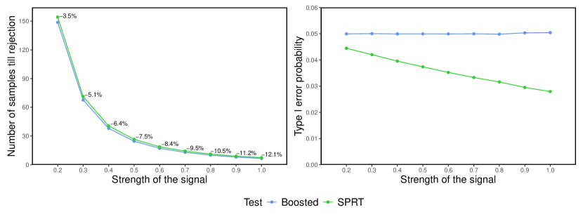
In Figure 1 we compare the SPRT with its boosted improvement regarding sample size and type I error in the simple Gaussian testing setup for different strengths of the signal $\delta$, where $\mu_{0}=0$. The results were obtained by averaging over $\numprint{10000}$ trials. In each trial, we generated up to $\numprint{10000}$ observations under the alternative until the hypothesis could be rejected by the respective sequential test. Both tests rejected the hypothesis in all cases. In order to determine the type I error for both of the methods, we used importance sampling by exploiting the fact [24] that

$\displaystyle\mathbb{P}_{\theta_{0}}(\tau<\infty)=\mathbb{E}_{\theta_{1}}\left[\mathbbm{1}\{\tau<\infty\}\Lambda_{\tau}^{-1}\right],$ (15)

where $\Lambda_{\tau}^{-1}$ is the likelihood ratio of $\theta_{0}$ to $\theta_{1}$ at time $\tau$. With this, we can estimate the type I error by the inverse of the likelihood ratio at the stopping time while sampling under the alternative. Since $\tau$ is almost surely finite and usually much smaller under the alternative than under the null hypothesis, this reduces the required number of samples to obtain a good estimate of the type I error [24, 25].

The boosting approach saves on average $4\%$ to $12\%$ of the sample size compared to the SPRT in the considered scenarios, while the percentage increases with the strength of the signal. Furthermore, the boosted SPRT exhausts the significance level, while the SPRT is becoming increasingly conservative for stronger signals.

Refer to caption
Figure 1: Comparison of sample size and type I error between the SPRT and the boosted SPRT in a simple Gaussian testing setup for different signal strengths. The boosted SPRT saves $4-12\%$ of sample size compared to the SPRT and exhausts the significance level. The SPRT is becoming increasingly conservative for stronger signals.

3.2 Handling composite alternatives with the predictable plugin method

In practice, a concrete alternative is often difficult to specify, leading to testing problems of the form

$$H_{0}:\theta^{*}=\theta_{0}\quad\text{vs.}\quad H_{1}:\theta^{*}>\theta_{0}.$$

There are two approaches that are usually used to handle such composite alternatives in sequential testing. The method of mixtures [19] and the predictable plugin [20, 21]. In the following, we will recap the latter, since it is better suited for our boosting technique.

Let $(\theta_{t})_{t\in\mathbb{N}}$ be a predictable process, meaning $\theta_{t}$ is measurable with respect to $\mathcal{F}_{t-1}$, such that $\theta_{t}\geq\theta_{0}$ for all $t\in\mathbb{N}$ and define

$\displaystyle\Lambda_{t}^{\text{plugin}}=\prod_{i=1}^{t}\frac{p_{\theta_{i}}(X_{i})}{p_{\theta_{0}}(X_{i})}.$ (16)

The idea of the predictable plugin method is to replace in the numerator of the likelihood ratio the density of a fixed alternative by an estimated density $p_{\theta_{t}}$ that is based on the previous data $X_{1},\ldots,X_{t-1}$. Since

$$\mathbb{E}_{\theta_{0}}\left[\frac{p_{\theta_{i}}(X_{i})}{p_{\theta_{0}}(X_{i})}\bigg{|}\Lambda_{i-1}^{\text{plugin}}\right]=\int_{\mathcal{X}}\frac{p_{\theta_{i}}(x)}{p_{\theta_{0}}(x)}p_{\theta_{0}}(x)\mu(dx)=\int_{\mathcal{X}}p_{\theta_{i}}(x)\mu(dx)=1,$$

it follows immediately that $(\Lambda_{t}^{\text{plugin}})$ defines a test martingale for $H_{0}$. Hence, the application of Algorithm 1 is straightforward. At each step $t\in\mathbb{N}$, we can calculate a boosting factor using (13) by just replacing $\theta_{1}$ with $\theta_{t}$.

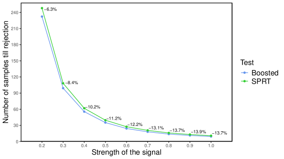
Robbins and Siegmund [21] introduced different estimators for the case of one-parameter exponential families and evaluated the expected sample size of the resulting sequential tests $\tau_{\text{plugin}}=\inf\{t\in\mathbb{N}:\Lambda_{t}^{\text{plugin}}\geq 1/\alpha\}$. A simple estimator they considered is $\theta_{1}=\theta_{0}$ and

$\displaystyle\theta_{t}=\max\left(\bar{X}_{t-1},\theta_{0}\right),$ (17)

where $\bar{X}_{t-1}=\sum_{i=1}^{t-1}X_{i}$. In Figure 2 we repeated the experiment from Figure 1 in Section 3.1 but assumed that the alternative is not specified in advance using the predictable parameter in (17). Unsurprisingly, the sample size required by both methods is larger than when the alternative was prespecified. However, the gain in sample size achieved by our boosting method is even larger in the case of the composite alternative, as we were able to save $6\%$ to $14\%$ of the sample size compared to the usual SPRT.

Refer to caption
Figure 2: Comparison of sample size between the SPRT with a predictable plugin and the boosted SPRT in a Gaussian testing setup with composite alternative for different signal strengths. The boosted SPRT saves $6-14\%$ of sample size compared to the SPRT.

3.3 Handling composite nulls in one-sided testing problems

An even more common testing setup in practice is

$$H_{0}:\theta^{*}\leq\theta_{0}\quad\text{vs.}\quad H_{1}:\theta^{*}>\theta_{0}\quad(\theta_{0}\in\Theta),$$

meaning we have a composite null hypothesis and a composite alternative. Robbins and Siegmund [20] showed that the process $Z_{t}$ defined in Equation (16) also provides a valid sequential test for the composite null hypothesis above. In the following, we show that the same holds for our boosted process.

Due to the monotone likelihood ratio property (12), we know that

$\displaystyle\mathbb{P}_{\theta_{0}}\left(\frac{p_{\theta_{t}}(X_{t})}{p_{\theta_{0}}(X_{t})}\geq x\right)\geq\mathbb{P}_{\theta}\left(\frac{p_{\theta_{t}}(X_{t})}{p_{\theta_{0}}(X_{t})}\geq x\right)\quad(\theta\leq\theta_{0},x\geq 0),$ (18)

where $\theta_{t}>\theta_{0}$. Writing $\lambda_{t}(X_{t})=\frac{p_{\theta_{t}}(X_{t})}{p_{\theta_{0}}(X_{t})}$, Equation (18) implies that

$$\mathbb{P}_{\theta_{0}}\left(T_{\alpha}(b_{t}\lambda_{t}(X_{t});M)\geq x\right)\geq\mathbb{P}_{\theta}\left(T_{\alpha}(b_{t}\lambda_{t}(X_{t});M)\geq x\right)\quad(\theta\leq\theta_{0},x\geq 0)$$

for any $\alpha\in(0,1)$, $M>0$ and $b_{t}\geq 1$. Hence, if $\mathbb{E}_{\theta_{0}}[T_{\alpha}(b_{t}\lambda_{t}(X_{t});M)|\Lambda_{t-1}^{\mathrm{boost}}]\leq 1$, we also have $\mathbb{E}_{\theta}[T_{\alpha}(b_{t}\lambda_{t}(X_{t});M)|\Lambda_{t-1}^{\mathrm{boost}}]\leq 1$ for all $\theta<\theta_{0}$. This implies that we can just use the likelihood ratio of $\theta_{t}$ vs. $\theta_{0}$ and derive the boosting factors by Algorithm 1 using $\mathbb{E}_{\theta_{0}}$, but the boosted test supermartingale will also be valid for all $\theta\leq\theta_{0}$.

To summarize, for the composite testing problem above we can do exactly the same as described in Section 3.2 for the simple null hypothesis while providing valid error control.

4 Nontrivial extensions and applications

In this section, we demonstrate some nontrivial extensions and applications of our boosting method. First, we show how it can be used for tighten confidence sequences in Section 4.1. Afterwards, we exemplify its use in sampling without replacement situations (Section 4.2) and with conformal martingales (Section 4.3) which are employed for testing the assumption of i.i.d. data.

4.1 Confidence sequences

A $(1-\alpha)$-level confidence sequence (CS) for some unknown parameter $\theta^{*}\in\Theta$ is a sequence of sets $(C_{t})_{t\in\mathbb{N}}$ such that

$\displaystyle\mathbb{P}_{\theta^{*}}(\exists t\in\mathbb{N}:\theta^{*}\notin C_{t})\leq\alpha.$ (19)

Let $\tau_{\theta}$, $\theta\in\Theta$, be a sequential test for $H_{0}^{\theta}:\theta^{*}=\theta$ with property (3). Then

$$C_{t}=\{\theta\in\Theta:\tau_{\theta}>t\}$$

is a CS for $\theta^{*}$. Let $(M_{t}^{\theta})$ be the test supermartingale for $H_{0}^{\theta}$ that defines $\tau_{\theta}$, meaning $\tau_{\theta}=\inf\{t\in\mathbb{N}:M_{t}^{\theta}\geq 1/\alpha\}$. It follows immediately that $(C_{t})_{t\in\mathbb{N}}$ can be boosted, meaning each $C_{t}$ shrinks in size while maintaining (19), by boosting each of the martingales $(M_{t}^{\theta})$, $\theta\in\Theta$, by Algorithm 1. However, the computational effort of this approach is extremely high or even infeasible.

Due to computational convenience and better interpretability, in practice one usually focuses on CSs that form an interval

$$C_{t}=(l_{t},u_{t})$$

for some lower bound $l_{t}$ and upper bound $u_{t}>l_{t}$. We will focus on the construction of a lower bound in the following. The two-sided CSs can then be obtained as the intersection of an upper and a lower $(1-\alpha/2)$-level confidence sequence. Hence, we are looking for a sequence $(l_{t})_{t\in\mathbb{N}}$ such that

$$\mathbb{P}_{\theta^{*}}(\exists t\in\mathbb{N}:\theta^{*}<l_{t})\leq\alpha.$$

In order to ensure that the resulting CS has this form, it is required that the martingales $(M_{t}^{\theta})_{\theta\in\Theta}$ are nonincreasing in $\theta$ for every $t\in\mathbb{N}$. Now note that each boosting factor $b_{t}^{\theta}$, $\theta\in\Theta$ and $t\in\mathbb{N}$, defined by Algorithm 1, is a nondecreasing function of the (boosted) supermartingale at the previous step $M_{t-1}^{\theta,\mathrm{boost}}$. Therefore, the boosting factors $(b_{t}^{\theta})_{\theta\in\Theta}$ are also nonincreasing in $\theta$. This implies that also the boosted processes $(M_{t}^{\theta,\mathrm{boost}})_{\theta\in\Theta}$ are nonincreasing in $\theta$ for each $t$ such that the resulting CS provides indeed a lower bound. With this, the boosted CS can be easily determined computationally by setting $l_{t}$ at each step $t\in\mathbb{N}$ to be the smallest $\theta\in\Theta$ such that $M_{t}^{\theta,\mathrm{boost}}<1/\alpha$. In the following, we illustrate the construction of a boosted CS with a Gaussian example.

Example 1.

Suppose we look for a confidence sequence for the mean $\mu^{*}$ of i.i.d. Gaussians $X_{1},X_{2},\ldots$ with known variance one. For each $\mu\in\mathbb{R}$, we need to determine a sequential test for the null hypothesis

$$H_{0}:\mu^{*}=\mu.$$

Let $\mu\in\mathbb{R}$ be fixed and define $Z_{t}=X_{t}-\mu$ for all $t\in\mathbb{N}$ such that each $Z_{t}$ is standard normally distributed under $H_{0}$. This implies that

$$\mathbb{E}_{\mu}[\exp(\delta Z_{t}-\delta^{2}/2)|\mathcal{F}_{t-1}]=1,$$

where $\delta>0$ is some constant. Hence, the process $(M_{t}^{\mu})$, where

$$M_{t}^{\mu}=\prod_{i=1}^{t}\exp(\delta Z_{i}-\delta^{2}/2)$$

provides a test martingale for $H_{0}$. Furthermore, note that $M_{t}^{\mu}$ is decreasing in $\mu$ for each $t$, such that the family of test martingales $((M_{t}^{\mu}))_{\mu\in\mathbb{R}}$ can be used to find a lower bound $l_{t}$ for $\mu^{*}$. Indeed, we can calculate

$\displaystyle M_{t}^{\mu}<1/\alpha\Leftrightarrow\prod_{i=1}^{t}\exp(\delta(X_{i}-\mu)-\delta^{2}/2)<1/\alpha\Leftrightarrow\frac{1}{t}\sum_{i=1}^{t}X_{i}-\frac{\log(1/\alpha)}{n\delta}-\delta/2<\mu.$

Consequently, $(l_{t})_{t\in\mathbb{N}}$, where $l_{t}=\frac{1}{t}\sum_{i=1}^{t}X_{i}-\frac{\log(1/\alpha)}{n\delta}-\delta/2$, is a valid lower bound sequence for $\mu^{*}$. By setting $Z_{t}=\mu-X_{t}$ one can derive an upper bound, yielding the $(1-\alpha)$ confidence sequence

$\displaystyle\frac{1}{t}\sum_{i=1}^{t}X_{i}\ \pm\ \left[\frac{\log(2/\alpha)}{t\delta}+\delta/2\right].$ (20)

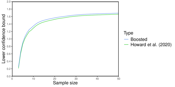
This CS was previously proposed by Howard et al. [10]. As described above, one can obtain a boosted confidence sequence numerically by boosting each $(M_{t}^{\mu})$, $\mu\in\mathbb{R}$, separately and choosing the smallest/largest $\mu\in\mathbb{R}$ such that $M_{t}^{\mu,\mathrm{boost}}<1/\alpha$ for the lower/upper bound. In Figure 3 we compare the $(1-\alpha)$ lower confidence bound proposed by Howard et al. [10] with our boosted improvement for $\mu^{*}=2$ (the bounds were obtained by averaging over $100$ trials), which shows that boosting can tighten the CS (20) significantly. We chose $\delta=\sqrt{8\log(1/\alpha)/n}$ for $n=50$, as recommended by Howard et al. [10] for obtaining a tight CS at time $n$.

Note that Howard et al. [10] proved that the CS (20) is valid for all 1-sub-Gaussian distributions. However, our boosting approach only ensures valid error control for Gaussian distributions with variance one. The reason is that

$$\mathbb{E}_{0}[L_{t}^{\prime}|\mathcal{F}_{t-1}]\leq\mathbb{E}_{0}[L_{t}|\mathcal{F}_{t-1}]\centernot\implies\mathbb{E}_{0}[T_{t}(b_{t}L_{t}^{\prime};M_{t-1}^{\mathrm{boost}})|\mathcal{F}_{t-1}]\leq\mathbb{E}_{0}[T_{t}(b_{t}L_{t};M_{t-1}^{\mathrm{boost}})|\mathcal{F}_{t-1}]$$

for $b_{t}>1$ and therefore it is not possible to handle all 1-sub-Gaussian distributions simultaneously. It is interesting that it is possible to exploit the information of the observations being exactly Gaussian (instead of just 1-sub-Gaussian), since previous works on confidence sequences did not make use of it [10, 11].

Refer to caption
Figure 3: Comparison of the lower confidence bound (20) by Howard et al. [10] with its boosted improvement for $\mu^{*}=2$. Boosting improves the CS significantly.

4.2 Sampling without replacement

Suppose we have some finite population $\{x_{1},\ldots,x_{N}\}$ and draw samples

$$X_{t}|\{X_{1},\ldots,X_{t-1}\}\sim\text{Uniform}(\{x_{1},\ldots,x_{N}\}\setminus\{X_{1},\ldots,X_{t-1}\})$$

sequentially and without replacement with the goal of testing the hypothesis

$$H_{0}:\mu^{*}\leq\mu_{0}\quad\text{vs.}\quad H_{1}:\mu^{*}>\mu_{0},$$

where $\mu^{*}=\frac{1}{N}\sum_{i=1}^{N}x_{i}$, because the effort of drawing all samples is too high. In this section, we focus on binary variables $X_{i}$. For example, this scenario is encountered when auditing the outcome of an election [41] or when checking whether the permutation p-value is below the predefined level $\alpha$ [40]. In the following, we show how the state-of-the-art method can be improved by our boosting technique.

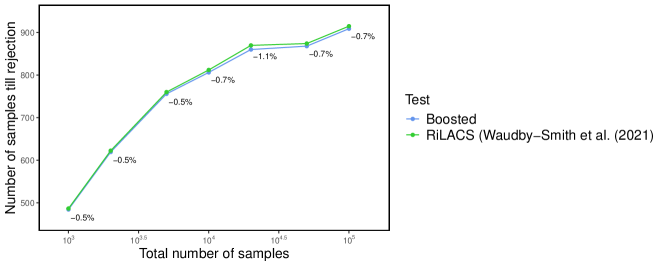
Waudby-Smith et al. [41] proposed the RiLACS algorithm to test $H_{0}$, which is based on the test martingale

$\displaystyle M_{t}=\prod_{i=1}^{t}(1+\lambda_{i}(X_{i}-C_{i}(\mu_{0}))),$ (21)

where $C_{i}(\mu_{0}))=\frac{N\mu_{0}-\sum_{j=1}^{i-1}X_{j}}{N-i+1}$ is the conditional mean of $X_{i}|X_{1},\ldots,X_{i-1}$ if the mean of $\{x_{1},\ldots,x_{N}\}$ is $\mu_{0}$ and $\lambda_{i}\in\left[0,\frac{1}{C_{i}(\mu_{0})}\right]$ is a hyperparameter measurable with respect to $\mathcal{F}_{i-1}$. Hence, each individual factor of $(M_{t})$ is just given by $L_{t}=1+\lambda_{i}(X_{i}-C_{i}(\mu_{0}))$. Under the null hypothesis and conditional on $\mathcal{F}_{t-1}$, we have that $L_{t}=1+\lambda_{i}(1-C_{i}(\mu_{0}))$ with probability at most $C_{i}(\mu_{0})$ and $L_{t}=1-\lambda_{i}C_{i}(\mu_{0})$ with probability at least $1-C_{i}(\mu_{0})$. This implies that we can determine valid boosting factors $b_{t}$ by

$\displaystyle b_{t}=\begin{cases}\frac{1-C_{i}(\mu_{0})/(M_{t-1}^{\mathrm{boost}}\alpha)}{(1-C_{i}(\mu_{0}))((1-\lambda_{i}C_{i}(\mu_{0}))},&\text{ if }M_{t-1}^{\mathrm{boost}}(1+\lambda_{i}(1-C_{i}(\mu_{0})))\geq 1/\alpha\\ 1,&\text{ otherwise.}\end{cases}$

If the alternative $H_{1}:\mu^{*}=\mu_{1}$ is known in advance, Waudby-Smith et al. [41] proposed to choose $\lambda_{i}=\min(1/C_{i}(\mu_{0}),2(2\mu_{1}-1))$. For example, this is the case in Risk-limiting audits (RLA) used for auditing the results of an election. In Figure 4, we compare the required sample size of RiLACS and its boosted improvement for $\mu_{0}=0.5$ and $\mu_{1}=0.55$ for different total number of samples $N$ at level $\alpha=0.01$. The gain in sample size obtained by boosting is small but visible. This is not surprising, since the RiLACS test martingale (21) only overshoots slightly at $1/\alpha$ due to the binary nature of the data.

Refer to caption
Figure 4: Comparison of the required sample size by RILACS [41] and its boosted improvement in a sampling without replacement setting for different total number of samples. Boosting leads to a visible gain in sample size. However, due to the binary nature of the data, overshoot is not that big of a problem and therefore the gain in sample size is smaller than in Gaussian examples.

4.3 Conformal martingales

A common assumption in statistics has been that the data is generated independently from the same distribution, also called iid. (independent and identically distributed). In this subsection, we consider testing this assumption sequentially, meaning to test the null hypothesis

$$H_{0}:X_{1},X_{2},\ldots\text{ are iid.}$$

From a single data sequence it is impossible to distinguish whether the data is iid or exchangeable [17], where $(X_{t})_{t\in\mathbb{N}}$ is called exchangeable if $(X_{1},\ldots,X_{t})$ has the same joint distribution as $(X_{\sigma(1)},\ldots,X_{\sigma(t)})$ for every $t\in\mathbb{N}$ and permutation $\sigma$ of the first $t$ indices. Hence, $H_{0}$ can be formulated equivalently as

$$H_{0}:X_{1},X_{2},\ldots\text{ are exchangeable.}$$

Note that this is a highly composite null hypothesis. However, Vovk’s conformal martingale approach [29, 32, 33] allows to reduce $H_{0}$ to a simple null hypothesis. This makes it not only possible to test $H_{0}$ sequentially using a test martingale, but also to apply our boosting technique from Algorithm 1. We first recap the method by Vovk and then demonstrate how we can apply our boosting approach on top of it.

Let $A$ be a nonconformity measure, which maps observations $(x_{1},\ldots,x_{t})$ of any length to a sequence of numbers $(z_{1},\ldots,z_{t})\in\mathbb{R}^{t}$ such that for any $t$ and any permutation $\sigma$ it holds that

$$A(x_{1},\ldots,x_{t})=(z_{1},\ldots,z_{t})\implies A(x_{\sigma(1)},\ldots,x_{\sigma(t)})=(z_{\sigma(1)},\ldots,z_{\sigma(t)}).$$

The number $z_{i}$ can be interpreted as the “strangeness” of $x_{i}$. With this, for each $t\in\mathbb{N}$, one can calculate a “p-value” by

$$p_{t}=\frac{|\{i\leq t:z_{i}>z_{t}\}|+\theta_{t}|\{i\leq t:z_{i}=z_{t}\}|}{t},$$

where $(z_{1},\ldots,z_{t})=A(x_{1},\ldots,x_{t})$ and $\theta_{t}$ is randomly and independently sampled from $U[0,1]$. Vovk showed that the p-values $p_{1},p_{2},\ldots$ are iid from $U[0,1]$ under the null hypothesis $H_{0}$.

Vovk proposed to collect evidence against $H_{0}$ by forming a conformal martingale $(M_{t})$ as

$$M_{t}=\prod_{i=1}^{t}f_{i}(p_{i}),$$

where $f_{i}:[0,1]\rightarrow[0,\infty]$, $i\in\mathbb{N}$, is a so called betting function with the property $\int_{0}^{1}f(u)du=1$ that may depend on the previous p-values. It is easy to check that this ensures $\mathbb{E}_{0}[f_{i}(p_{i})|M_{t-1}]=1$ such that $(M_{t})$ is indeed a test martingale for $H_{0}$ and $f_{i}(p_{i})$ are the corresponding individual factors. Note that $(M_{t})$ may not be a martingale with respect to the filtration generated by the observations $X_{1},X_{2},\ldots$, but it surely is with respect to the filtration generated by the p-values $p_{1},p_{2},\ldots$ .

A concrete betting function proposed by Vovk is

$$f_{\kappa}(u)=\kappa u^{\kappa-1},\quad\kappa\in(0,1).$$

Since we know that the p-values $p_{1},p_{2},\ldots$ are iid uniformly distributed on $U[0,1]$ under $H_{0}$, we can easily determine the distribution of $f_{\kappa}(p_{i})$ conditional on the previous p-values for every $\kappa$ such that Algorithm 1 can be applied. For example, $\alpha=0.05$, $M_{t-1}^{\mathrm{boost}}=1$ and $\kappa=0.5$ yield a boosting factor of $b_{t}=1.013$. The boosting factor is decreasing in $\kappa$ such that we obtain a boosting factor of $b_{t}=2.199$ for $\kappa=0.1$.

5 Avoiding conservatism with two-sided thresholds

While the previous sections focused on power-one SPRTs where we only stop to reject the null but not to accept it, we now consider the case where we also wish to stop if it is unlikely that we would reject the null if we continued testing. We will show how we can use a similar boosting technique as in Section 2 to construct powerful anytime-valid tests that allow to stop for futility.

Suppose our test is based on the test (super)martingale $(M_{t})$. We consider stopping for futility (and accepting the null) if $M_{t}\leq\nu_{t}$, where $\nu_{t}<1/\alpha$ is a predictable parameter, meaning $\nu_{t}$ is measurable with respect to $\mathcal{F}_{t-1}$. For example, Wald’s approximation suggests to set $\nu_{t}=\frac{\beta}{1-\alpha}$. Note that stopping for futility can never increase the type I error, but it may hurt the power. Below, we will show how we can gain back part of that power.

If $M_{t}>0$, we have $\mathbb{E}_{0}[M_{t^{\prime}}|\mathcal{F}_{t}]=M_{t}>0$ for all $t^{\prime}>t$. Hence, if we stop when our test martingale is strictly positive, we make a conservative decision since there is a positive probability of rejecting if we continue sampling. Therefore, our approach is to form a truncated test (super)martingale $(M_{t}^{\mathrm{trunc}})$ such that $M_{t}^{\mathrm{trunc}}\leq\nu_{t}$ implies that $M_{t}^{\mathrm{trunc}}=0$. To achieve this, we extend our truncation function $T_{\alpha}(x;M)$ from (8) as follows

$\displaystyle T_{\alpha}(x;M,\nu)=\begin{cases}0,&\text{ if }Mx\leq\nu\\ x,&\text{ if }\nu<Mx\leq\frac{1}{\alpha}\\ \frac{1}{M\alpha},&\text{ if }Mx>\frac{1}{\alpha}.\end{cases}$ (22)

Note that $T_{\alpha}(x;M,\nu)=T_{\alpha}(x;M)$, if $\nu=0$. Furthermore, $T_{\alpha}(x;M,\nu)\leq T_{\alpha}(x;M)$ for all $x\in\mathbb{R}_{\geq 0}$, implying that the boosting factors obtained by $T_{\alpha}(x;M,\nu)$ are larger than the boosting factors computed with $T_{\alpha}(x;M)$. We can use $T_{\alpha}(x;M,\nu)$ for boosting in the same manner as we did for $T_{\alpha}(x;M)$ in Algorithm 1. The following corollary extends Theorem 2.1 by including the futility stop.

Corollary 5.1.

Let $(M_{t})$ be any test (super)martingale and $(M_{t}^{\mathrm{boost}})$ be the process obtained by applying Algorithm 1 with $T_{\alpha}(x;M_{t-1}^{\mathrm{boost}},\nu_{t})$ and define the sequential tests $\delta_{M}=\mathbbm{1}\{M_{\tau_{M}}\geq 1/\alpha\}$ and $\delta_{\mathrm{boost}}=\mathbbm{1}\{M_{\tau_{\mathrm{boost}}}^{\mathrm{boost}}\geq 1/\alpha\}$, where $\tau_{M}=\inf\{t\in\mathbb{N}:M_{t}\geq 1/\alpha\lor M_{t}\leq\nu_{t}\}$ and $\tau_{\mathrm{boost}}=\inf\{t\in\mathbb{N}:M_{t}^{\mathrm{boost}}\geq 1/\alpha\lor M_{t}^{\mathrm{boost}}\leq\nu_{t}\}$. Then $M_{t}^{\mathrm{boost}}\geq M_{t}$ for all $t<\tau_{M}$ and $\delta_{\mathrm{boost}}\geq\delta$ almost surely. Furthermore, $(M_{t}^{\mathrm{boost}})$ is a test supermartingale. Therefore, $\mathbb{P}_{0}(\delta_{\mathrm{boost}}=1)\leq\alpha$ and $\mathbb{E}_{0}[M_{\tau}^{\mathrm{boost}}]\leq 1$ for all stopping times $\tau$.

Note that in contrast to Theorem 2.1, Corollary 5.1 does not show that the boosted test $(\delta_{\mathrm{boost}},\tau_{\mathrm{boost}})$ stops earlier than the initial test $(\delta_{M},\tau_{M})$. The problem is that the boosted process is always larger than the initial test until a decision is obtained and therefore may continue sampling while the initial test has already stopped for futility. But, the boosted process never stops later for rejecting the null hypothesis. Therefore, one could obtain a uniform improvement $(\delta^{\prime},\tau^{\prime})$ of $(\delta_{M},\tau_{M})$, meaning $\delta^{\prime}\geq\delta$ and $\tau^{\prime}\leq\tau$ almost surely, by $\delta^{\prime}=\mathbbm{1}\{M_{\tau^{\prime}}^{\mathrm{boost}}\geq 1/\alpha\}$ where $\tau^{\prime}=\min(\tau_{M},\tau_{\mathrm{boost}})$. However, the test $(\delta^{\prime},\tau^{\prime})$ might stop while the boosted supermartingale is strictly positive, meaning it is conservative.

In the same manner as in Equation (13), we can calculate for power-one SPRTs

$\displaystyle\mathbb{E}_{\theta_{0}}[T_{\alpha}(b_{t}\lambda(X_{t});\Lambda_{t-1}^{\mathrm{boost}},\nu_{t})|\Lambda_{t-1}^{\mathrm{boost}}]$ $\displaystyle=b_{t}\left[F_{\theta_{1}}\left(\lambda^{-1}\left([b_{t}\alpha\Lambda_{t-1}^{\mathrm{boost}}]^{-1}\right)\right)-F_{\theta_{1}}\left(\lambda^{-1}\left(\nu_{t}/[b_{t}\Lambda_{t-1}^{\mathrm{boost}}]\right)\right)\right]$
$\displaystyle+(\Lambda_{t-1}^{\mathrm{boost}}\alpha)^{-1}\left[1-F_{\theta_{0}}\left(\lambda^{-1}\left(\left[b_{t}\alpha\Lambda_{t-1}^{\mathrm{boost}}\right]^{-1}\right)\right)\right].$

The boosting factors obtained in the same setup as for Table 1, but with a stop for futility at $\nu_{t}=0.4$, is shown in Table 2. Obviously, all boosting factors are larger when the stop for futility is included. Furthermore, especially in cases where the current martingale value $\Lambda_{t-1}^{\mathrm{boost}}$ is small, including the stop for futility increases the boosting factor.
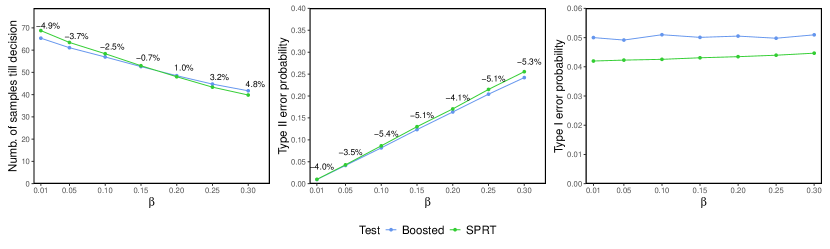
$\delta$ $\Lambda_{t-1}^{\mathrm{boost}}$ $0.5$ $1$ $2$ $4$ $10$
$0.1$ $1.00895$ $1$ $1$ $1$ $1.00001$
$0.5$ $1.17964$ $1.01743$ $1.00026$ $1.00019$ $1.03019$
$1$ $1.21801$ $1.07547$ $1.02817$ $1.05651$ $1.37357$
$2$ $1.32013$ $1.38991$ $1.62094$ $2.21769$ $5.76214$
$3$ $2.73073$ $3.75762$ $6.00201$ $12.1467$ $68.8295$
Table 2: Boosting factors obtained for $\alpha=0.05$ and $\nu_{t}=0.4$, $t\in\mathbb{N}$, in a simple Gaussian testing problem with mean difference $\delta$ and variance $1$.

There are many choices for $\nu_{t}$ one could make. For example, one could choose $\nu_{t}=\frac{\beta}{1-\alpha}\prod_{i=1}^{t-1}b_{i}$, where the $b_{i}$ are the previous boosting factors and $\beta\in(0,1)$ is the desired type II error probability. In this case, the true type II error probability is similar to the one obtained by the SPRT with Wald’s approximations, since $\Lambda_{t}^{\mathrm{boost}}\leq\nu_{t}\implies\Lambda_{t}\leq\frac{\beta}{1-\alpha}$. In Figure 5, we compare the sample size, the type II and the type I error probability of the SPRT with our boosted method for different parameters $\beta$ in the same Gaussian simulation setup as considered in Section 3.1 (the type I error probability was obtained via importance sampling, see (15)). The desired type I error probability was set to $\alpha=0.05$ and the strength of the signal to $\delta=0.3$. Note that the boosted method leads to a lower type II error in all cases. Furthermore, it reduces the sample size when $\beta$ is small ($<0.2$), which is the usual case in most applications. For $\beta\geq 0.2$, the sample size was smaller using the SPRT. However, in these cases the boosted method led to a significantly smaller type II error probability. Hence, the sample size obtained with the boosted method could possibly be reduced by choosing a larger stop for futility $\nu_{t}$, while retaining a similar type II error probability as the SPRT. The boosted SPRT approximately exhausted the type I error probability while the SPRT is conservative.

Refer to caption
Figure 5: Comparison of sample size, type II and type I error probability between the SPRT and the boosted SPRT in a simple Gaussian testing setup for different desired type II error probabilities ($\beta$). The boosted method saves sample size when $\beta$ is small while reducing the type II error probability. Furthermore, the boosted SPRT approximately exhausts the type I error level $\alpha=0.05$.
Remark 4.

Note that our boosted SPRT could also be written as

$$\text{reject }H_{0},\text{ if }\Lambda_{t}\geq\gamma_{1}^{t},\quad\text{accept }H_{0},\text{ if }\Lambda_{t}\leq\gamma_{0}^{t},\quad\text{and continue sampling if }\gamma_{0}^{t}<\Lambda_{t}<\gamma_{1}^{t},$$

where $\gamma_{1}^{t}=\frac{1}{\alpha\prod_{i=1}^{t}b_{i}}$ and $\gamma_{0}^{t}=\frac{\nu_{t}}{\prod_{i=1}^{t}b_{i}}$ are predictable parameters. Such generalized SPRTs with non-constant boundaries over time were already introduced by Weiss [42], however, Weiss assumed that $\gamma_{0}^{t}$ and $\gamma_{1}^{t}$, $t\in\mathbb{N}$, are prespecified constants.

Remark 5.

If we choose $\gamma_{0}=\beta$ and $\gamma_{1}=1/\alpha$, then the SPRT provably controls the type I and type II error [34, 35] (but is usually conservative). Hence, if we apply our boosted SPRT with $\nu_{t}=\beta\prod_{i=1}^{t-1}b_{i}$, we also control the type I and type II error, since we control the type I error by construction and are uniformly more powerful than the SPRT with $\gamma_{0}=\beta$ and $\gamma_{1}=1/\alpha$.

6 Discussion

6.1 Testing a forecaster

The classical SPRT by Wald [34, 35] assumes that the null hypothesis and the alternative hypothesis are specified in advance in the form of simple distributions $\mathbb{P}_{0}$ and $\mathbb{P}_{1}$, respectively. However, in Section 3.2 we have seen that the SPRT remains even valid if we replace the fixed alternative $\mathbb{P}_{1}$ with a predictable plugin $\mathbb{P}_{1}^{t}$ that depends on the data $X_{1},\ldots,X_{t-1}\in\mathcal{X}$ observed so far. In general, the null distribution $\mathbb{P}_{0}^{t}$ and the alternative distribution $\mathbb{P}_{1}^{t}$ considered at each step $t\in\mathbb{N}$ can be chosen freely based on the previous data $X_{1},\ldots,X_{t-1}$ and some additional information $Z_{1},\ldots,Z_{t}\in\mathcal{Z}$. Shafer [22] formulated this as a forecaster-sceptic testing protocol, where the forecaster announces a probability distribution $\mathbb{P}_{0}^{t}$ at each step $t$ and a sceptic tests the forecaster by specifying an alternative $\mathbb{P}_{1}^{t}$. For example, one can think of the forecaster as a weather forecaster, which is tried to be invalidated by a sceptic. We summarized this general testing protocol in Algorithm 2.

The extension of our boosting technique (Algorithm 1) to the general testing problem in Algorithm 2 is straightforward, since at each step $t$ we only require the current martingale value $M_{t-1}=\Lambda_{t-1}$ and the distribution of the next factor $L_{t}=\frac{\mathbb{P}_{1}^{t}(X_{t})}{\mathbb{P}_{0}^{t}(X_{t})}$ under the null hypothesis $\mathbb{P}_{0}^{t}$.

Algorithm 2 SPRT in a general forecaster-sceptic testing protocol

Input: Lower and upper SPRT thresholds $\gamma_{0}$ and $\gamma_{1}$.
      Output: Decision on the forecaster.

1:$\Lambda_{0}=1$
2:for $t=1,2,\ldots$ do
3:     Reality announces $Z_{t}\in\mathcal{Z}$
4:     Forecaster announces a probability distribution $\mathbb{P}_{0}^{t}$ on $\mathcal{X}$
5:     Sceptic announces a probability distribution $\mathbb{P}_{1}^{t}$ on $\mathcal{X}$
6:     Reality announces $X_{t}\in\mathcal{X}$
7:     $\Lambda_{t}=\Lambda_{t-1}\cdot\frac{\mathbb{P}_{1}^{t}(X_{t})}{\mathbb{P}_{0}^{t}(X_{t})}$
8:     if $\Lambda_{t}\geq\gamma_{1}$ then
9:         Stop and reject the forecaster
10:     end if
11:     if $\Lambda_{t}\leq\gamma_{0}$ then
12:         Stop and accept the forecaster
13:     end if
14:end for

6.2 Other approaches to avoid Wald’s approximated thresholds

The problem of “overshoot” in the SPRT was already noted by Wald [34, 35] and examined in many previous works. One line of work approximates the exact type I and type II error of SPRTs based on Brownian motion and renewal theory [23, 25, 3, 12, 43, 15]. While the resulting approximations are asymptotically correct, they are very difficult to compute and therefore only used rarely in practice [23, 25]. For example, we have already seen that the available R packages for performing an SPRT [27, 2] rely on Wald’s approximated thresholds and that most applied studies also use them (e.g. [26, 13, 4, 9]). Another option is to truncate the SPRT by prespecifying a maximum number of observations. For simple distributions of the likelihood ratio and sufficiently small maximum numbers of observations it is then possible to calculate the type I and type II error for given thresholds exactly [1], which can be used to find appropriate bounds for the SPRT. Such an approach is frequently employed in group sequential trials [14, 39]. For more complex distributions one could approximate the error probabilities using Monte-Carlo sampling. This often leads to considerably computational effort, which sometimes can be reduced using importance sampling [24]. A limitation these three approaches have in common is that the used test statistics including their distributions must be specified in advance. This is not necessarily the case in the general forecaster-sceptic testing protocol described in the previous section. Hence, while our boosting approach is applicable to such complex and adaptive testing protocols, all of the aforementioned methods fail.

6.3 Improving (sequential) tests based on e-values

A recently popularized tool for sequential statistics is the e-value [18, 22, 8, 30]. An e-value for a null hypothesis $H_{0}:\mathbb{P}\in\mathcal{P}$, where $\mathcal{P}$ is some set of distributions, is a nonnegative random variable with expected value less or equal than one for all $\mathbb{P}\in\mathcal{P}$. For example, a likelihood ratio for a simple null hypothesis is an e-value. Therefore, e-values can be interpreted as generalized likelihood ratios for composite null hypotheses [22, 8]. When used for testing, e-values suffer from the same conservativeness due to overshoot as test martingales. It is conceptually straightforward to extend our boosting approach to general e-values theoretically by ensuring that (10) holds for all $\mathbb{P}\in\mathcal{P}$, although it might be difficult to calculate boosting factors in practice, depending on the complexity of $\mathcal{P}$. However, in Section 3.3 we at least showed that it is possible to apply it with the composite null hypotheses resulting from one-sided tests for exponential families.

7 Summary

In this paper, we introduced a general approach to uniformly improve nonnegative (super)martingale based sequential tests by avoiding an overshoot at the upper threshold $1/\alpha$ (where $\alpha$ is the desired type-I error). We illustrated its application by the power-one SPRT with one-parameter exponential families for one-sided null and alternative hypotheses. We also showed how it can be applied when a lower threshold is specified, that determines an early stopping time for accepting the null hypothesis. With this we obtain an alternative to the two-sided SPRT with Wald’s approximated thresholds, where our alternative provides valid type I error control and leads to similar type II error as Wald’s proposal while often reducing the sample size. Our sequential tests can also be used to tighten confidence sequences and be extended to nontrivial settings like sampling without replacement and conformal martingales.

Acknowledgments

LF acknowledges funding by the Deutsche Forschungsgemeinschaft (DFG, German Research Foundation) – Project number 281474342/GRK2224/2. AR was funded by NSF grant DMS-2310718.

References

  • Armitage et al. [1969] Peter Armitage, CK McPherson, and BC Rowe. Repeated significance tests on accumulating data. Journal of the Royal Statistical Society: Series A (General), 132(2):235–244, 1969.
  • Bottine [2015] Stephane Mikael Bottine. SPRT: Wald’s Sequential Probability Ratio Test, 2015. URL https://CRAN.R-project.org/package=SPRT. R package version 1.0.
  • Chan and Lai [2000] Hock Peng Chan and Tze Leung Lai. Asymptotic approximations for error probabilities of sequential or fixed sample size tests in exponential families. Annals of statistics, pages 1638–1669, 2000.
  • Chetouani [2014] Yahya Chetouani. A sequential probability ratio test (sprt) to detect changes and process safety monitoring. Process Safety and Environmental Protection, 92(3):206–214, 2014.
  • Chow et al. [1971] Yuan Shih Chow, Herbert Robbins, and David Siegmund. Great Expectations: The theory of optimal stopping. Houghton Mifflin Company, Boston, 1971.
  • Darling and Robbins [1968] Donald A Darling and Herbert Robbins. Some nonparametric sequential tests with power one. Proceedings of the National Academy of Sciences, 61(3):804–809, 1968.
  • Grünwald et al. [2023] Peter Grünwald, Alexander Henzi, and Tyron Lardy. Anytime-valid tests of conditional independence under model-X. Journal of the American Statistical Association, pages 1–12, 2023.
  • Grünwald et al. [2024] Peter Grünwald, Rianne de Heide, and Wouter M Koolen. Safe testing. Journal of the Royal Statistical Society Series B: Statistical Methodology (with discussion), 2024.
  • Hapfelmeier et al. [2023] Alexander Hapfelmeier, Roman Hornung, and Bernhard Haller. Efficient permutation testing of variable importance measures by the example of random forests. Computational Statistics & Data Analysis, 181:107689, 2023.
  • Howard et al. [2020] Steven R Howard, Aaditya Ramdas, Jon McAuliffe, and Jasjeet Sekhon. Time-uniform chernoff bounds via nonnegative supermartingales. Probability Surveys, 17:257–317, 2020.
  • Howard et al. [2021] Steven R Howard, Aaditya Ramdas, Jon McAuliffe, and Jasjeet Sekhon. Time-uniform, nonparametric, nonasymptotic confidence sequences. Annals of Statistics, 2021.
  • Hu [1988] Inchi Hu. Repeated significance tests for exponential families. The Annals of Statistics, 16(4):1643–1666, 1988.
  • Ivan Chang [2004] Yuan-chin Ivan Chang. Application of sequential probability ratio test to computerized criterion-referenced testing. Sequential Analysis, 23(1):45–61, 2004.
  • Jennison and Turnbull [1999] Christopher Jennison and Bruce W Turnbull. Group sequential methods with applications to clinical trials. CRC Press, 1999.
  • Lai and Siegmund [1977] Tze L Lai and David Siegmund. A nonlinear renewal theory with applications to sequential analysis i. The Annals of Statistics, pages 946–954, 1977.
  • Ramdas et al. [2020] Aaditya Ramdas, Johannes Ruf, Martin Larsson, and Wouter Koolen. Admissible anytime-valid sequential inference must rely on nonnegative martingales. arXiv preprint arXiv:2009.03167, 2020.
  • Ramdas et al. [2022] Aaditya Ramdas, Johannes Ruf, Martin Larsson, and Wouter M Koolen. Testing exchangeability: Fork-convexity, supermartingales and e-processes. International Journal of Approximate Reasoning, 141:83–109, 2022.
  • Ramdas et al. [2023] Aaditya Ramdas, Peter Grünwald, Vladimir Vovk, and Glenn Shafer. Game-theoretic statistics and safe anytime-valid inference. Statistical Science, 38(4):576–601, 2023.
  • Robbins [1970] Herbert Robbins. Statistical methods related to the law of the iterated logarithm. The Annals of Mathematical Statistics, 41(5):1397–1409, 1970.
  • Robbins and Siegmund [1972] Herbert Robbins and David Siegmund. A class of stopping rules for testing parametric hypotheses. Proc. Sixth Berkeley Symrp. Math. Statist, 1972.
  • Robbins and Siegmund [1974] Herbert Robbins and David Siegmund. The expected sample size of some tests of power one. The Annals of Statistics, 2(3):415–436, 1974.
  • Shafer [2021] Glenn Shafer. Testing by betting: A strategy for statistical and scientific communication. Journal of the Royal Statistical Society Series A: Statistics in Society (with discussion), 184(2):407–431, 2021.
  • Siegmund [1975] D Siegmund. Error probabilities and average sample number of the sequential probability ratio test. Journal of the Royal Statistical Society: Series B (Methodological), 37(3):394–401, 1975.
  • Siegmund [1976] David Siegmund. Importance sampling in the monte carlo study of sequential tests. The Annals of Statistics, pages 673–684, 1976.
  • Siegmund [1985] David Siegmund. Sequential analysis: tests and confidence intervals. Springer Science & Business Media, 1985.
  • Spiegelhalter et al. [2003] David Spiegelhalter, Olivia Grigg, Robin Kinsman, and TOM Treasure. Risk-adjusted sequential probability ratio tests: applications to bristol, shipman and adult cardiac surgery. International Journal for Quality in Health Care, 15(1):7–13, 2003.
  • Steinhilber et al. [2023] Meike Steinhilber, Martin Schnuerch, and Anna-Lena Schubert. sprtt: Sequential Probability Ratio Tests Toolbox, 2023. URL https://CRAN.R-project.org/package=sprtt. R package version 0.2.0.
  • Ville [1939] Jean Ville. Etude critique de la notion de collectif. Gauthier-Villars Paris, 1939.
  • Vovk [2021] Vladimir Vovk. Testing randomness online. Statistical Science, 36(4):595–611, 2021.
  • Vovk and Wang [2021] Vladimir Vovk and Ruodu Wang. E-values: Calibration, combination and applications. The Annals of Statistics, 49(3):1736–1754, 2021.
  • Vovk and Wang [2024] Vladimir Vovk and Ruodu Wang. Merging sequential e-values via martingales. Electronic Journal of Statistics, 18(1):1185–1205, 2024.
  • Vovk et al. [2005] Vladimir Vovk, Alexander Gammerman, and Glenn Shafer. Algorithmic learning in a random world, volume 29. Springer, 2005.
  • Vovk et al. [1999] Volodya Vovk, Alexander Gammerman, and Craig Saunders. Machine-learning applications of algorithmic randomness. In Proceedings of the Sixteenth International Conference on Machine Learning, pages 444–453, 1999.
  • Wald [1945] A Wald. Sequential tests of statistical hypotheses. The Annals of Mathematical Statistics, 16(2):117–186, 1945.
  • Wald [1947] A. Wald. Sequential Analysis. J. Wiley & Sons, New York, 1947.
  • Wald [1944] Abraham Wald. On cumulative sums of random variables. The Annals of Mathematical Statistics, 15(3):283–296, 1944.
  • Wald and Wolfowitz [1948] Abraham Wald and Jacob Wolfowitz. Optimum character of the sequential probability ratio test. The Annals of Mathematical Statistics, pages 326–339, 1948.
  • Wang and Ramdas [2022] Ruodu Wang and Aaditya Ramdas. False discovery rate control with e-values. Journal of the Royal Statistical Society Series B: Statistical Methodology, 84(3):822–852, 2022.
  • Wassmer and Brannath [2016] Gernot Wassmer and Werner Brannath. Group sequential and confirmatory adaptive designs in clinical trials, volume 301. Springer, 2016.
  • Waudby-Smith and Ramdas [2020] Ian Waudby-Smith and Aaditya Ramdas. Confidence sequences for sampling without replacement. Advances in Neural Information Processing Systems, 33:20204–20214, 2020.
  • Waudby-Smith et al. [2021] Ian Waudby-Smith, Philip B Stark, and Aaditya Ramdas. Rilacs: risk limiting audits via confidence sequences. In Electronic Voting: 6th International Joint Conference, E-Vote-ID 2021, Virtual Event, October 5–8, 2021, Proceedings 6, pages 124–139. Springer, 2021.
  • Weiss [1953] Lionel Weiss. Testing one simple hypothesis against another. The Annals of Mathematical Statistics, pages 273–281, 1953.
  • Woodroofe [1976] Michael Woodroofe. A renewal theorem for curved boundaries and moments of first passage times. The Annals of Probability, 4(1):67–80, 1976.