Enhancing SNN-based Spatio-Temporal Learning: A Benchmark Dataset and Cross-Modality Attention Model

Abstract

Spiking Neural Networks (SNNs), renowned for their low power consumption, brain-inspired architecture, and spatio-temporal representation capabilities, have garnered considerable attention in recent years. Similar to Artificial Neural Networks (ANNs), high-quality benchmark datasets are of great importance to the advances of SNNs. However, our analysis indicates that many prevalent neuromorphic datasets lack strong temporal correlation, preventing SNNs from fully exploiting their spatio-temporal representation capabilities. Meanwhile, the integration of event and frame modalities offers more comprehensive visual spatio-temporal information. Yet, the SNN-based cross-modality fusion remains underexplored.

In this work, we present a neuromorphic dataset called DVS-SLR that can better exploit the inherent spatio-temporal properties of SNNs. Compared to existing datasets, it offers advantages in terms of higher temporal correlation, larger scale, and more varied scenarios. In addition, our neuromorphic dataset contains corresponding frame data, which can be used for developing SNN-based fusion methods. By virtue of the dual-modal feature of the dataset, we propose a Cross-Modality Attention (CMA) based fusion method. The CMA model efficiently utilizes the unique advantages of each modality, allowing for SNNs to learn both temporal and spatial attention scores from the spatio-temporal features of event and frame modalities, subsequently allocating these scores across modalities to enhance their synergy. Experimental results demonstrate that our method not only improves recognition accuracy but also ensures robustness across diverse scenarios.

1 Introduction

The spiking neural network (SNN), as a promising brain-inspired computational model, has garnered considerable attention in recent years. Event cameras, a type of neuromorphic vision sensor, generate a stream of asynchronous events only after detecting intensity changes. This characteristic aligns naturally with the event-driven, spike-based, and spatio-temporal representation property of SNNs.

The datasets captured by event cameras are known as neuromorphic vision datasets. A suitable benchmark dataset is crucial for fairly evaluating improved algorithms and advancing the development of SNNs. Nonetheless, many studies have highlighted the shortcomings of current SNN datasets. (He et al., 2020) compared the performance of SNNs and RNNs under different workloads and found that SNNs have a distinct advantage in high temporal resolution workloads—a feature not supported by many existing datasets. (Iyer et al., 2021) conducted unsupervised RD-STDP (Reward-Dependent Spike-Timing-Dependent Plasticity) and STDP-tempotron methods on the N-MNIST dataset and discovered that temporal information does not play a significant role in classification for N-MNIST; even when the event stream is accumulated into a single frame, the accuracy does not decrease significantly. (Deng et al., 2020) found that the performance of SNNs on some neuromorphic datasets was even inferior to ANNs and underscored the urgent need to create more SNN-oriented datasets.

In this work, we designed two experiments called Spike Timing Confusion and Temporal Information Elimination to quantify and analyze the importance of temporal information. Our analysis indicates that many prevalent neuromorphic datasets lack sufficient temporal correlation, preventing SNNs from fully exploiting their spatio-temporal representation capabilities. Building on these findings, we believe that an appropriate benchmark dataset would enable SNNs to fully exploit the characteristics of spatio-temporal representation and rapid response, allowing SNNs to demonstrate their distinctiveness (Li et al., 2022). To this end, we design and record a sign language action recognition dataset using the DAVIS346 event camera. To date, it is the most extensive action recognition neuromorphic dataset, featuring 21 sign language action segments performed by 43 participants under three lighting conditions and two position conditions, with a total recording time exceeding 9 hours. To validate its optimal use of spatio-temporal properties of SNNs, we carry out Spike Timing Confusion and Temporal Information Elimination experiments. The former jumbles the spike timings of the input event stream, feeding the model erroneous temporal information, while the latter accumulates the entire event stream spatially into one frame, preventing the model from accessing temporal information. Experimental results suggest our dataset has higher temporal correlation and increased recognition difficulty. We underscore that it is not necessary for researchers to pursue the marginal performance improvement of SNN on ANN-oriented datasets, but to tackle some problems that render more challenges to ANNs. Our dataset can better exploit the inherent properties of SNNs, thus paving the way for fair comparisons between SNN algorithms and exploration of spatio-temporal properties.

On the other hand, event modality is difficult to represent background and texture information. Integrating event modality with traditional color frame modality can facilitate a more holistic understanding of a visual scene. Such integration has been successfully applied to target tracking (Luo et al., 2022; Wang et al., 2021), image reconstruction (Paikin et al., 2021; Tulyakov et al., 2022), SLAM (Weikersdorfer et al., 2014; Cheng et al., 2022), and more. However, most of these applications are based on ANNs and ignore the rich temporal information captured in the event modality. Due to the lack of dual-modal datasets and the inherent complexities of the neurodynamics, the development of SNN-based modality fusion techniques has been impeded.

As such, we synchronously recorded the corresponding color frame data when capturing the neuromorphic dataset. Based on this dual-modal dataset, we introduce a Cross-Modality Attention (CMA) module and establish a baseline for SNN-based fusion. This module is designed end-to-end and can be seamlessly integrated into SNN framework. It comprises two distinct components: the spatial-wise CMA and the temporal-wise CMA. For the spatial-wise CMA, it first computes the spatial-wise spike rate of the frame features. The spike rate can be interpreted as the degree of response to specific information. Subsequently, a learnable 2D nonlinear convolutional mapping is executed, producing spatial attention scores. These scores are then cross-fused with event features, resulting in spatially enhanced features. In parallel, the temporal-wise CMA undergoes a similar procedure. It begins by determining the temporal-wise spike rate of the event features. Subsequently, a learnable nonlinear 1D fully-connected mapping is employed to yield temporal attention scores, which are then cross-fused with frame features to craft temporally enhanced features. We conducted detailed experiments under various latency parameters and scenario settings. Our experimental results show that the integration of CMA not only improves the recognition accuracy but also enables the model maintaining robustness under diverse conditions. Furthermore, The efficacy of the CMA module is confirmed through a comprehensive ablation study.

In summary, our contributions are as follows:

1. [(1)]

2. We introduce a benchmark neuromorphic dataset. Compared to other commonly used datasets, it can better enable SNNs to exploit their inherent properties, especially in terms of spatio-temporal representation. Additionally, it encompasses frame data synchronized with the event stream, making it suitable for developing SNN-based fusion techniques.

3. We delve deeply into the inadequacies of current neuromorphic datasets in terms of temporal correlation, an aspect that many previous studies have highlighted but not thoroughly investigated. Through conducting Spike Timing Confusion and Temporal Information Elimination experiments, we substantiate that our dataset exhibits a higher degree of temporal correlation, establishing it as a appropriate benchmark for SNN evaluations.

4. We introduce a Cross-Modality Attention (CMA) model that captures both temporal and spatial attention scores from the spatio-temporal features in event and frame modalities. These scores are then cross-allocated to the other modality, enhancing the synergy between them.

2 Related Works

2.1 Spiking Neural Network

Unlike ANNs, each neuron in an SNN accumulates incoming signals over time. When the accumulated signal surpasses a given threshold, the neuron ’fires’, or produces a binary spike, and resets. This dynamic allows SNNs to encode and process information both spatially and temporally (Gerstner et al., 2014). Moreover, the inherent event-driven characteristics of SNNs allow for faster response and lower power consumption, making them highly suitable for tasks requiring real-time responses (Bouvier et al., 2019).

However, the introduction of spiking neurons results in the non-differentiable nature of SNNs, rendering conventional backpropagation optimization unsuitable for training SNNs directly. To address this issue, researchers have explored two main approaches.

One approach involves initially training the desired model using ANNs. Given a pre-trained ANN, ANN-SNN conversion involves substituting the activation function with spiking neurons, accompanied by meticulous parameter adaptation, to replicate the continuous feature representation via spiking neurons (Diehl et al., 2015, 2016; Han et al., 2023; Qu et al., 2024). Some studies optimize the intrinsic spatiotemporal dynamics of spiking neurons to achieve low latency and sparse computing (Zhang et al., 2023, 2021). A large amount of recent work has demonstrated that the performance of converted SNNs is comparable to ANNs over large-scale datasets (Fang et al., 2021; Bu et al., 2023; Hao et al., 2023; Rueckauer et al., 2017; Wang et al., 2023). However, the converted SNNs are unable to process continuous inputs due to the limitations of the original ANN input formats.

Another approach aims to train SNNs directly by introducing the concept of surrogate gradients, which make the non-differentiable process of spike firing derivable. A significant advancement in this domain is the Spatio-Temporal Back Propagation (STBP) method (Wu et al., 2019), which combines the principles of Back Propagation Through Time (Werbos, 1990) with surrogate gradient techniques, showing promising results. Further developments in neuron models (Fang et al., 2021; Yu et al., 2022; Ma et al., 2023), network architectures (Hu et al., 2021; Fang et al., 2021; Yao et al., 2021; Feng et al., 2022), and training techniques (Xie et al., 2023; Hu et al., 2021; Zheng et al., 2021; Yang et al., 2022; Wang et al., 2023; Gu et al., 2019) underscore the immense potential of SNNs. This direct training approach is inherently adept at managing continuous inputs, potentially paving the way for advancements in fields such as action recognition (Liu et al., 2021; Gao et al., 2023), target tracking (Cao et al., 2015), mapless navigation (Yang et al., 2023), trajectory prediction (Debat et al., 2021), object detection (Yu et al., 2024; Yuan et al., 2024),and more.

2.2 Neuromorphic Datasets

Neuromorphic datasets are specialized datasets developed to train and test neuromorphic computing systems, such as SNNs. These datasets encode information in an event-driven manner, where each "event" signifies a spike generated by a neuron at a specific moment in time. These datasets can encompass various types of data including but not limited to images, sounds (Anumula et al., 2018), or other sensor data (See et al., 2020; Vanarse et al., 2022). This discussion is limited to neuromorphic vision datasets.

Neuromorphic vision datasets can generally be divided into three categories based on their source and generation methods: (i) Simulated Datasets, (ii) Converted Datasets, and (iii) Real-World Datasets.

Among them, the simulated datasets are directly generated from existing video streams (or images) using specific difference algorithms (Rebecq et al., 2018) or frame-based generation algorithms (Hu et al., 2021) to create a neuromorphic version of the original data. These datasets are generally used to provide additional dynamic information to assist in tasks such as tracking (Wang et al., 2021; Zhang et al., 2023), depth estimation (Gehrig et al., 2021), optical flow estimation (Li et al., 2023), image reconstruction (Wang et al., 2019), and more. However, a significant downside is the inability to accurately emulate event-driven characteristics, attributed to the limited frame rate of conventional videos. Consequently, it fails to correctly reflect real-time spatio-temporal information, thereby offering restricted support in fostering the progress of SNNs.

The converted datasets refer to neuromorphic datasets formulated from well-established datasets in the ANN domain; notable examples include N-MNIST (Orchard et al., 2015) derived from MNIST, N-ImageNet (Kim et al., 2021) from ImageNet, and DVS-CIFAR10 (Li et al., 2017) from CIFAR10, among others (Lin et al., 2021; Hu et al., 2016). Generally, the creation of these datasets entails initially stabilizing the original images, followed by moving the event camera along a predetermined path, thereby generating a corresponding event stream version. However, these datasets, despite meeting the formal prerequisites for SNNs, are not genuinely neuromorphic in nature. Our research (see Section 5.1) indicates that the precise spike timing of these datasets bears negligible influence on the accuracy, and the total elimination of temporal information does not cause a marked decrease in performance. Hence, these datasets fall short in fully harnessing the spatio-temporal representation potential inherent in SNNs, making them unsuitable as benchmark datasets for SNN evaluations. This standpoint is echoed by numerous other studies in the field (Iyer et al., 2021; He et al., 2020; Deng et al., 2020).

The real-world datasets are recorded by event cameras in actual scenes. Compared to the aforementioned methods, the data acquired in this manner is authentic and natural, directly reflecting the motion of objects and the spatio-temporal characteristics in the real environments, offering immense value for the advancement of SNNs. This type of datasets has already been widely used for gesture recognition (Amir et al., 2017; Vasudevan et al., 2021; Miao et al., 2019; Liu et al., 2021; Dong et al., 2022), and object classification (Serrano-Gotarredona and Linares-Barranco, 2015; Sironi et al., 2018). However, with the rapid advancements in SNNs, the existing datasets have become inadequate for fostering the further development of SNNs. For instance, the most frequently utilized DVS-Gesture dataset (Amir et al., 2017) is now too simplistic for the current approaches of SNNs, allowing an easy attainment of about 95% recognition accuracy. Moreover, these datasets are unimodal, offering no assistance in the research of spatio-temporal fusion techniques in SNNs and lacking a corresponding color frame based baseline for comparison.

2.3 Collaboration of Event and Frame Modalities

Traditional frame-based cameras excel at providing rich details concerning background and texture. However, they suffer from motion blur when capturing high-speed moving objects and have a lower dynamic range. Event cameras can overcome these shortcomings by offering a higher temporal resolution and dynamic range, supplying complementary dynamic information to the frame stream (Gehrig et al., 2021).

In the early stages, researchers envisioned the potential of fusing these two modalities for video processing (Leow and Nikolic, 2015). Following this, with the advancement of deep neural networks, researchers began to leverage the benefits of this fusion in more specialized applications such as SLAM (Weikersdorfer et al., 2014; Cheng et al., 2022), image reconstruction (Paikin et al., 2021; Tulyakov et al., 2022), monocular depth estimation (Gehrig et al., 2021), object tracking (Luo et al., 2022; Wang et al., 2021), object localization (Lele et al., 2022), semantic segmentation (Natan and Miura, 2021), and image enhancement (Bi et al., 2023).

Nevertheless, the majority of these cases utilize the event stream merely as an auxiliary modality, aiming to alleviate the deficiencies in the frame modality, particularly their low temporal resolution and limited dynamic range. These approaches predominantly rely on ANNs and often necessitate complex preprocessing and crafted designs, bypassing the direct engagement with spatio-temporal feature modeling. In this work, we aim to propose an end-to-end fusion strategy, which is tailored to the unique characteristics of each modality and facilitates seamless integration within the SNN framework.

3 DVS-SLR Benchmark Dataset

With the rapid development of neuron models, network architectures, and training techniques, there is an urgent need for SNN-oriented benchmark datasets (Deng et al., 2020). We align with (Iyer et al., 2021; He et al., 2020; Li et al., 2022) in the viewpoint that most of the so-called "neuromorphic" datasets are not quite "neuromorphic". Although their data format aligns with the event-driven nature of SNNs, the temporal information contained may not be significant enough. Moreover, these datasets are uni-modal, offering no assistance in the research of modality fusion techniques in SNNs and lacking a corresponding color-frame based baseline for comparison.

As such, we designed and recorded a dual-modal neuromorphic dataset. This dataset serves two purposes. When its event modality is used alone, it can act as a more suitable benchmark dataset for SNN evaluation, as it has higher temporal correlation and can fully exploit the spatio-temporal nature of SNNs. When used in its dual-modal form, it can assist in the development and validation of SNN-based fusion methods.

In this section, we will introduce the dataset’s design, the recording process, and its analysis.

3.1 Dataset Design

The output of a neuron in a SNN at any given timestep depends on the current input and the state of the neuron. The neuron’s state carries information from the past. This computational paradigm endows SNNs with an intrinsic ability for temporal modeling. Additionally, information is transmitted in the form of spikes (0 or 1) in SNNs, enabling them to operate at lower power consumption and with faster response times. Considering these attributes, an ideal benchmark dataset or task should highlight the importance of both temporal and spatial information (Li et al., 2022; Iyer et al., 2021), and the input data should be continuous. Additionally, the benchmark task should be straightforward and simple, without requiring complex data preprocessing.

Action recognition, reliant on subtle variations in spatio-temporal sequences and sparse data processing, naturally aligns with the properties of SNNs, making it an ideal benchmark task for SNNs. While there are existing neuromorphic datasets for action recognition (Amir et al., 2017; Vasudevan et al., 2021; Miao et al., 2019; Liu et al., 2021), they fall short in scale, diversity, and difficulty, and lack corresponding frame data. To circumvent these issues, we designed our dataset with the following considerations: (1) Large-scale: It is well-known that large-scale datasets can facilitate the development of more complex models. Our dataset surpasses previously commonly used datasets in scale. It comprises 5418 samples recorded by 43 subjects, each lasting about 6 seconds, totaling over 9 hours of recording. (2) Multi-illumination: Compared to conventional frame cameras, event cameras possess a higher dynamic range and perform well under low-light conditions. Introducing a variety of illumination conditions increases data diversity and promotes the exploration of modality fusion. We have designed three lighting conditions: bright LED light, dim LED light, and natural light. (3) Multiple positions: The distance between the subjects and the camera results in different event rates and spatial distributions, contributing to sample diversity. (4) Dual-modality: Most existing datasets are uni-modal, lacking a corresponding color-frame based baseline for comparison and inhibiting the development of SNN-based fusion techniques. Hence, we opted for the DAVIS346 camera, capable of synchronously outputting both event streams and frame streams. A comparison of the parameters of commonly used neuromorphic cameras is shown in Table 1.

Table 1: Comparison of Commonly Used Event Cameras

Camera	Reference	Resolution	Latency ($\mu s$)	Dynamic range (dB)	Dual-modality	Color frame
DVS128	(Lichtsteiner et al., 2008)	$128\times 128$	12	120	no	no
ATIS	(Posch et al., 2010)	$240\times 304$	3	143	yes	no
DAVIS346	(Inivation, 2019)	$260\times 346$	20	120	yes	yes

3.2 Dataset Recording

Figure 1: The recording environment.

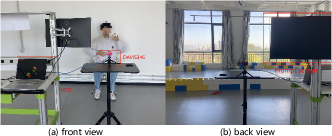
Figure 1 shows the recording environment. The DAVIS346 camera was fixed on the desk, facing the subjects. Each subject was required to record six sets of data under three illumination conditions (natural light, bright LED light, dim LED light) and from two positions (front, back). Before recording each set of data, the staff would adjust the lighting and the position of the seat. The positions "front" and "back" are approximately $1.5m$ and $1m$ from the camera, respectively. Under natural light conditions, the curtains were fully opened, resulting in light intensities ranging from 300 to 850 lux, varying with the time of day and weather. For the LED light scenarios, the curtains were drawn closed, and we employed high-power LED strips and low-power LED bulbs to create bright and dim lighting environments, with respective light intensities of about 300lx and 150lx.

Although the DAVIS346 camera is capable of achieving frame rates of up to 40fps, such a short exposure time in dim LED light conditions causes the APS(Active Pixel Sensor) to produce almost black images. Therefore, we set a consistent frame rate of 20fps, which produces a color frame every 0.05 seconds. To collect data from the DAVIS346 camera, we initiated two ROS (Robot Operating System) nodes, one for events and one for frames. These nodes process data from the camera and broadcast it over designated ROS topics. With the rosbag utility in ROS, we recorded these topic messages into a .bag file. Considering the variety of actions, it was unrealistic to expect each subject to memorize them all. To assist, our system displayed a 3-second instructional video on a prompt screen (see Figure 1) before recording each action, which the subjects were to mimic. After the instructional video concluded, the recording session began, continuing until the start of the next instructional video.

We selected 20 standard actions from Chinese Sign Language, including you, I, everybody, at, go, want, listen, talk, see, run, jump, study, eat, drink, wash hands, shower, rest, sleep, home, and school. These actions encompass various motion trajectories and hand postures. Compared to other action recognition datasets, our actions are semantically rich and hence more complex. We also introduced an OTHER category for gestures improvised by the subjects, enhancing sample diversity. To ensure diversity in the dataset, we imposed no specific requirements on the speed of the action, the participant’s dominant hand, sitting posture, clothing, or hand positioning. For further details, please visit our webpage.

3.3 Dataset Analysis

Figure 2: Event frequency of each category in different scenarios. Event frequency refers to the number of events per second, measured in 1,000 events/s.

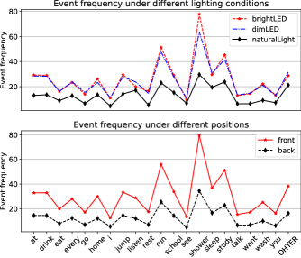
To input asynchronous event streams into SNNs, most studies use a method based on accumulating events over fixed time intervals into frames. A rich distribution of event frequencies helps increase sample diversity and enhance the model’s generalization performance.

Figure 3: Event frequency distribution of samples from different subjects. Event frequency is measured in 1,000 events/s.

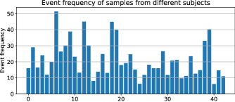
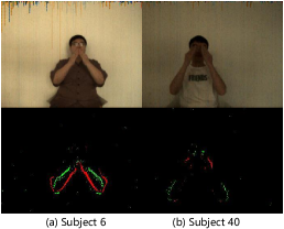
To enhance the diversity of our dataset, we designed various scenarios. Below, we analyze the diversity introduced by these designs. As shown in Figure 2, the event frequency under bright LED and dim LED lighting conditions does not differ significantly, while it decreases under natural light. This is partly because the relative change in light intensity is less pronounced under natural light than under LED light, resulting in fewer events captured by the event camera. Additionally, the imperceptible flickering of LED lights leads to a substantial number of events captured. The event frequency is higher in the "front" position than in the "back" position because the subject occupies more pixels in the front position. Furthermore, as seen in Figure 3, there is considerable variation in the event frequency of samples produced by different subjects. The highest event frequency is from subject 6, and the lowest is from subject 40, attributed to the higher contrast between subject 6’s clothing and the background (see Figure 4), which triggers more events.

Figure 4: Sample comparison from different subjects. (a) Sample from subject 6, with a higher event frequency. (b) Sample from subject 40, with a lower event frequency.

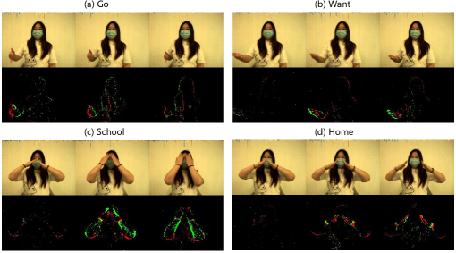
Some of the selected sign language actions are prone to confusion. Some actions share similar trajectories but differ in hand postures (e.g., "want" vs. "go"), while others differ in trajectories but have similar hand postures (e.g., "school" vs. "home"). Figure 5 illustrates these confusing similarities.

Figure 5: Comparison of different actions. (a) and (b) have the same hand motion trajectory but different hand postures. (c) and (d) have the same hand posture, forming a "roof-like" shape with both hands, but different motion trajectories.

Table 2: Comparison of Neuromorphic Datasets for Action Recognition. Abbreviations: SS - Sample Size, NC - Number of Classes, AD - Average Duration, TRT - Total Recording Time, ML - Multi-light, MP - Multi-position, DM - Dual-Modality

Dataset	Reference	Resolution	SS	NC	AD	TRT	ML	MP	DM
DVS-Gesture	(Amir et al., 2017)	$128\times 128$	1342	11	5s	1.86h	$\times$	$\times$	$\times$
SL-Animal-DVS	(Vasudevan et al., 2021)	$128\times 128$	1121	19	4.5s	1.4h	$\times$	$\times$	$\times$
ActionRecognition	(Miao et al., 2019)	$260\times 346$	291	10	5s	0.4h	$\times$	✓	$\times$
DailyAction	(Liu et al., 2021)	$260\times 346$	1440	12	5s	2h	$\times$	✓	$\times$
DVS-SLR (Ours)	-	$260\times 346$	5418	21	6s	9.03h	✓	✓	✓

Table LABEL:table_datasets compares our dataset with other commonly used neuromorphic datasets for action recognition. Our DVS-SLR dataset has the advantages of larger scale, multiple scenarios, and dual-modality. We anticipate that this dataset will pave the way for fair evaluation of SNNs and the development of SNN-based fusion methods.

4 Methods

4.1 Data Preprocessing

Data Preprocessing of Event Modality. Event cameras generate an asynchronous stream of events, which is not directly compatible with neural network inputs. Typically, these events are processed by being accumulated into frames. Consider a segment of an event stream, where each event $e$ is characterized by ($x,y,t,p$), with $x,y$ indicating the spatial coordinates of the event, $t$ its timestamp, and $p$ its polarity. Polarity is usually represented as +1 (signifying an increase in brightness) or -1 (indicating a decrease in brightness). The construction of the accumulated frame is as follows:

$$I_{0}(x,y) =\sum_{e\in E_{0}}\delta(p-1)\cdot\delta(x-x_{e})\cdot\delta(y-y_{e}),$$ (1)

$$I_{1}(x,y) =\sum_{e\in E_{1}}\delta(p+1)\cdot\delta(x-x_{e})\cdot\delta(y-y_{e}),$$ (2)

where $I\in{\mathbb{R}^{2\times H\times W}}$ denotes the derived accumulated frame, consisting of two channels: $E_{0}$ for frames crafted from positive polarity events and $E_{1}$ for negative polarity events. The function $\delta(\cdot)$ is the Dirac delta function, which returns 1 when its arguments match and 0 otherwise.

Figure 6: The process of temporal sampling. (a) When $dt$ surpasses the frame interval, the frame stream undergoes upsampling, utilizing adjacent frames to fill the gaps. (b) Conversely, if $dt$ is lower than the frame interval, the frame stream is subjected to downsampling, preserving only the most recent frames.

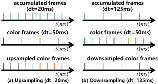
Dual-Modality Alignment and Sampling. Our dataset is dual-modal, with the frame modality’s frame interval set at 50ms during recording. Since the temporal resolution of the event stream is much higher than that of the frame stream, a smaller time window (e.g., $dt$ < 50ms) is often chosen when accumulating the event stream into frames, leading to asynchrony between the two modalities. To synchronize both modalities, we sample the color frames. As depicted in Figure 6, when $dt$ < 50$ms$, the module retains only the latest color frame, discarding prior ones. Conversely, if $dt$ > 50$ms$, the module fills missing frames using the most recent color frame.

In this study, we employ the LIF neuron model for neuronal modeling due to its optimal balance between precision and computational complexity. Specifically, its dynamics are given by:

$$\left\{\begin{gathered}\tau\frac{{du}}{{dt}}=-u+I,u<{V_{th}}\hfill\\ {\text{fire a spike \& }}u\leftarrow{u_{reset}},{\text{ }}u\geqslant{V_{th}}\hfill\\ \end{gathered}\right.$$ (3)

where $u$ is the membrane potential, $\tau$ is the time constant, and $I$ is the input synaptic current. Given that the above equation is continuous, for its application in deep learning frameworks, we leverage the Euler formula for its expansion and simplification:

$$u^{t+1}=(\frac{\tau-1}{\tau})u^{t}+\frac{1}{\tau}I.$$ (4)

The pre-synaptic input $I$ is then approximated through a linear summation of the pre-synaptic spikes (Wu et al., 2019):

$$u^{t+1}=(\frac{\tau-1}{\tau})u^{t}+\sum_{j}W_{j}o(j),$$ (5)

where $j$ indicates the index of pre-synapse. Incorporating the firing-and-resetting mechanism delineated in Eq. (3), we have:

$$\begin{array}[]{l}u^{t+1,n+1}(i)=(\frac{\tau-1}{\tau})u^{t,n+1}(i)(1-o^{t,n+1}(i))+\sum\limits_{j=1}^{l(n)}w_{ij}^{n}o^{t+1,n}(j),\\ o^{t+1,n+1}(i)=f(u^{t+1,n+1}(i)-V_{th}),\\ \end{array}$$ (6)

where $n$ and $l(n)$ signify the layer index and its corresponding neuron count. The synaptic weight between the $j$-th neuron of the preceding layer $(n)$ and the $i$-th neuron of the subsequent layer $(n+1)$ is denoted by $w_{ij}$. The function $f(\cdot)$ represents the Heaviside function: when $x<0$, $f(x)=0$; otherwise, $f(x)=1$.

4.2 Baseline Model

Figure 7: The architecture of our uni-modality baseline model. This model comprises the Spiking Conv Encoder, Spiking FC Decoder, and Voting Module. Unlike traditional CNNs, information in SNNs is transmitted along both the temporal and spatial dimensions.

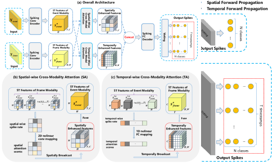
For a novel dataset, a simple yet robust baseline model serves to provide subsequent researchers with a performance yardstick, motivating them to devise superior methodologies to surpass this benchmark. Inspired by the architecture proposed in (Fang et al., 2021), our baseline model comprises three key components: the Spiking Conv Encoder, the Spiking FC (Fully Connected) Decoder, and the Output module (see Figure 7).

The Spiking Conv Encoder consists of $N_{conv}$ sets of Conv2D-BN (Batch Normalization)-LIF (Leaky Integrate-and-Fire) -Maxpool2D modules. All Conv2D layers have a kernel size of 3, stride of 1, and padding of 1. Each pooling layer employs a kernel size of 2 and a stride size of 2.

The Spiking FC Decoder is composed of $N_{fc}$ sets of FC-Dropout-LIF modules. The last FC layer has $N$ neurons, where $N$ should be a multiple of the class count $C$. The sparse output spikes are then directed into a voting module to produce the final output.

The Voting Module is designed to relieve the challenges posed by the sparse nature of spikes. For each timestep, it processes the incoming $N$ spikes, dividing them along the spatial dimension into $C$ groups, and subsequently computes the average value for each group as the final output of the current timestamp.

4.3 Fusion Strategy

Figure 8: Illustration of Accumulated Frame characteristics. Top-left: Slow hand wave from right to left; Top-right: Fast hand wave from right to left; Bottom-left: Slow hand wave from left to right; Bottom-right: Fast hand wave from left to right. In this illustration, green and red pixels indicate negative and positive event polarities, respectively. Motion vectors are annotated within the images for reference. During movement, negative events come before positive ones. This pattern hints at the direction of movement. Also, faster movements create more events within a given duration (dt), suggesting that the event frequency conveys, in part, the speed of the movement.

Figure 9: Illustration of Color Frame Characteristics. The action shown at the top signifies "go", while the one at the bottom represents "want". Despite both actions exhibiting a similar cyclical arm movement from the front to the back, they differ in hand gestures. In instances like these, the frame modality, compared to the event modality, offers richer texture details, enhancing the extraction of discriminative features.

4.3.1 Analysis of Modality Complementarity

Effective action recognition systems integrate both temporal and spatial features, harnessing the strengths of each to build robust models. Modern deep learning approaches, especially those leveraging two-stream architectures (Simonyan and Zisserman, 2014; Carreira and Zisserman, 2017; Feichtenhofer et al., 2019), have shown good performance. We draw inspiration from these successful approaches in two main aspects:

1. [(1)]

2. Two-stream architectures employ convolutional kernels that extend into the temporal dimension. This allows the convolutional networks to effectively extract temporal features. In contrast, our approach leverages the intrinsic temporal modeling of SNNs, eliminating the need for 3D convolution operations.

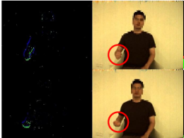
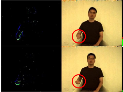
3. Two-stream architectures utilize inputs that are complementary. Apart from the traditional frame stream, they introduce optical flow into the system. However, its computational demand often limits its use in real-time applications. In our design, we view the event modality and the frame modality as complementary. The event stream implicitly reflects the motion direction and speed of the object (see Figure 8). On the other hand, the frame stream captures detailed spatial features, such as shape, texture, and color of objects (see Figure 9).

Nevertheless, seamlessly integrating both within the SNNs framework remains a challenging endeavor.

4.3.2 Cross-modality Attention

Figure 10: Schematic of the cross-modality fusion based action recognition framework. (a) depicts the overall framework, where the Spiking Conv Encoder, Spiking FC Decoder, and Output module all originate from the baseline model. (b) and (c) detail the spatial-wise and temporal-wise cross-modality attention module, respectively.

Drawing from our analysis, event streams excel at capturing dynamic changes, whereas frame streams provide more extensive spatial information. Embracing these distinct characteristics, our fusion approach seeks to extract temporal attention scores from the event modality and spatial attention scores from the frame modality, subsequently cross-fusing them to enhance the synergy between the two. Inspired by the Convolutional Block Attention Module (CBAM) (Woo et al., 2018) and Attention Spiking Neural Networks (Yao et al., 2023), we employ Temporal Attention (TA) and Spatial Attention (SA) to generate attention scores. Intuitively, TA instructs the network on when to pay attention, while SA indicates where to pay attention. Figure 10 visually represents this process. The spike firing rate reflects the neurons’ activity intensity and can be interpreted as the degree of response to specific information (Salinas and Sejnowski, 2000). To augment the learning of attention scores, unlike (Yao et al., 2023), which uses the membrane potential as the input, we employ the spike firing rate as the input to our attention module.

Formally, let $s_{e}^{n}\in{\mathbb{R}^{T\times C\times H_{n}\times W_{n}}}$ and $s_{f}^{n}\in{\mathbb{R}^{T\times C\times H_{n}\times W_{n}}}$ denote the spatio-temporal features of the event and frame modalities, respectively. Here, $n$ is the layer index for the final convolutional block, $T$ represents the timesteps, and $H_{n}$, $W_{n}$, and $C$ are the height, width, and channel dimensions of the feature map at layer $n$.

For the event modality, the temporal spike firing rate is defined as $r_{e}^{n}=[\cdots,r_{e}^{t,n}\cdots]\in{\mathbb{R}^{T}}$, and can be computed for each timestep as:

$$r_{e}^{t,n}=\frac{1}{{C\times{H_{n}}\times{W_{n}}}}\sum\limits_{k}^{C}{\sum\limits_{i}^{{H_{n}}}{\sum\limits_{j}^{{W_{n}}}{s_{e}^{t,n}(k,i,j)}}}.$$ (7)

In parallel, the spatial spike firing rate for the frame modality is denoted by $r_{f}^{n}={\left\{{r_{f}^{n}(i,j)}\right\}_{{H_{n}}\times{W_{n}}}}\in{\mathbb{R}^{{H_{n}}\times{W_{n}}}}$, and for each spatial position, it’s computed as:

$$r_{f}^{n}(i,j)=\frac{1}{{T\times C}}\sum\limits_{t}^{T}{\sum\limits_{k}^{C}{s_{f}^{n}(t,k,i,j)}}.$$ (8)

Then, the temporal attention scores ${d_{e}^{n}}\in{\mathbb{R}^{T}}$ are learned through two nonlinear FC mappings:

$$d_{e}^{n}=\sigma(M_{2}^{n}\delta(M_{1}^{n}r_{e}^{n})),$$ (9)

where $M_{1}^{n}\in{\mathbb{R}^{T\times\frac{T}{r}}}$ and $M_{2}^{n}\in{\mathbb{R}^{\frac{T}{r}\times T}}$ are learnable parameters, $\delta$ and $\sigma$ represent the sigmoid and ReLU function.

Similarly, the spatial attention scores, denoted as ${d_{f}^{n}}\in{\mathbb{R}^{{H_{n}}\times{W_{n}}}}$, are learned through a convolutional mapping:

$$d_{f}^{n}=\sigma(M_{3}^{n}*r_{f}^{n}),$$ (10)

where the $M_{3}^{n}\in{\mathbb{R}^{3\times 3}}$ signifies a learnable convolution kernel, $\sigma$ represents the ReLU function, and $*$ indicates the convolution operation. Subsequently, temporal attention scores and frame features are cross-fused to yield temporally augmented features, $\tilde{s}_{f}^{n}=[\cdots,\tilde{s}_{f}^{t,n}\cdots]\in{\mathbb{R}^{T\times C\times{H_{n}}\times{W_{n}}}}$. Explicitly, the fusion for each timestep is given by:

$$\tilde{s}_{f}^{t,n}=d_{e}^{t,n}\times s_{f}^{t,n}.$$ (11)

In a mirrored operation, spatial attention scores and event features are cross-fused, resulting in spatially augmented features, $\tilde{s}_{e}^{n}\in{\mathbb{R}^{T\times C\times{H_{n}}\times{W_{n}}}}$. For each spatial coordinate, the fusion is:

$$\tilde{s}_{e}^{n}(:,:,i,j)=d_{f}^{n}(i,j)\times s_{e}^{n}(:,:,i,j).$$ (12)

Finally, the cross-modality augmented features are concatenated, yielding the final CMA module output:

$${{\tilde{s}}^{n}}=[\tilde{s}_{e}^{n};\tilde{s}_{f}^{n}]\in{\mathbb{R}^{T\times 2C\times{H_{n}}\times{W_{n}}}}.$$ (13)

In order to make it clear to the reader, we have also presented the computation processes for TA and SA modules in pytorch pseudocode form, as illustrated in Algorithm 1 and 2.

Algorithm 1 Temporal Attention Fusion

1:Input:

2: $s_{e}[T,C,H,W]$: Event modality features

3: $s_{f}[T,C,H,W]$: Frame modality features

4:

5:Output:

6: $TempEnh[T,C,H,W]$: Temporally enhanced features

7:

8:Begin:

9:// Compute Temporal Spike Firing Rate for event modality

10:$r_{e}\leftarrow\text{mean}(s_{e},\text{axis}=(C,H,W))$ // Dimensions: [T]

11:

12:// Compute Temporal Attention Scores (TA)

13:$TA\leftarrow\sigma(M_{2}^{n}\cdot\delta(M_{1}^{n}\cdot r_{e}))$ // Dimensions: [T]

14:

15:// Apply Temporal Attention to frame features using broadcasting and multiplication

16:// Dimensions: [T, C, H, W]

17:$TempEnh\leftarrow TA.unsqueeze(1).unsqueeze(2).unsqueeze(3)\cdot s_{f}$

18:End

Algorithm 2 Spatial Attention Fusion

1:Input:

2: $s_{e}[T,C,H,W]$: Event modality features

3: $s_{f}[T,C,H,W]$: Frame modality features

4:

5:Output:

6: $SpaEnh[T,C,H,W]$: Spatially enhanced features

7:

8:Begin:

9:// Compute Spatial Spike Firing Rate for frame modality

10:$r_{f}\leftarrow\text{mean}(s_{f},\text{axis}=(T,C))$ // Dimensions: [H, W]

11:

12:// Compute Spatial Attention Scores (SA)

13:$SA\leftarrow\sigma(\text{Convolve}(M_{3},r_{f}))$ // Dimensions: [H, W]

14:

15:// Apply Spatial Attention to event features using broadcasting and multiplication

16:// Dimensions: [T, C, H, W]

17:$SpaEnh\leftarrow SA.unsqueeze(0).unsqueeze(0)\cdot s_{e}$

18:End

4.4 Overall Training

The overall architecture is illustrated in Figure 10. Its fundamental components are the same as the baseline model, but with the addition of dual-modality input and CMA module. The model receives synchronized dual-modality inputs, $X_{event}\in{\mathbb{R}^{T\times 2\times H\times W}}$ and $X_{frame}\in{\mathbb{R}^{T\times 3\times H\times W}}$. Each modality’s data is input into the Spiking Conv Encoder to extract spatio-temporal features. These features are then fed into the spatial-wise CMA and temporal-wise CMA for cross-modality fusion. The fused features are concatenated and fed into the Spiking FC Decoder and Voting Module to produce the output spikes.

Formally, let $T$ denote the timesteps, and $C$ represent the number of classes. For each input, the network produces an output $O={\left\{{o_{i}^{t}}\right\}_{T\times C}}$. Ideally, for an input labeled $l$, the neuron corresponding to the correct class should fire at every timestep, with other neurons remaining inactive. This target behavior can be expressed mathematically as:

$$y_{i}^{t}=\left\{\begin{array}[]{ll}1&\text{if }i=l\\ 0&\text{if }i\neq l\end{array}\right.$$ (14)

The discrepancy between the predicted output and this target is captured using the mean squared error (MSE) as loss function:

$$L=\frac{1}{{T\times C}}\sum\limits_{t}{\sum\limits_{i}{{{(o_{i}^{t}-y_{i}^{t})}^{2}}}}.$$ (15)

Furthermore, the predicted label $\hat{l}$ corresponds to the neuron’s index showcasing the utmost spike firing rate, defined as $\hat{l}=\arg{\max_{i}}\sum\limits_{t}{o_{i}^{t}}$.

In this study, we utilize STBP (Wu et al., 2019) to train our network. The gradient is back-propagated simultaneously across both temporally and spatially:

$$\frac{{\partial L}}{{\partial o_{i}^{t,n}}} =\sum\limits_{j=1}^{l(n+1)}{\frac{{\partial L}}{{\partial o_{j}^{t,n+1}}}}\frac{{\partial o_{j}^{t,n+1}}}{{\partial o_{i}^{t,n}}}+\frac{{\partial L}}{{\partial o_{i}^{t+1,n}}}\frac{{\partial o_{i}^{t+1,n}}}{{\partial o_{i}^{t,n}}},$$ (16)

$$\frac{{\partial L}}{{\partial u_{i}^{t,n}}} =\frac{{\partial L}}{{\partial o_{i}^{t,n}}}\frac{{\partial o_{i}^{t,n}}}{{\partial u_{i}^{t,n}}}+\frac{{\partial L}}{{\partial o_{i}^{t+1,n}}}\frac{{\partial o_{i}^{t+1,n}}}{{\partial u_{i}^{t,n}}},$$ (17)

where $l(n+1)$ denotes all the neurons in the $(n+1)$th layer.

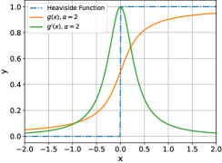
The firing process in SNNs is inherently non-differentiable. We approximate the Heaviside function using:

$$g(x)=\frac{1}{\pi}{\text{arctan}}\left(\frac{\pi}{2}\alpha x\right)+\frac{1}{2}$$ (18)

Its derivative or the surrogate gradient can be expressed as:

$$g^{\prime}(x)=\frac{{dg}}{{dx}}=\frac{\alpha}{{2(1+\left(\frac{\pi}{2}\alpha x\right)^{2})}}$$ (19)

Figure 11 provides a visual representation of the Heaviside function, its approximation $g(x)$, and the surrogate gradient ${g^{\prime}}(x)$. Although the surrogate gradient isn’t an exact representation, it offers a commendable approximation of the spike firing behavior and its efficacy has been substantiated in numerous studies (Zheng et al., 2021; Zhang and Li, 2020; Yang et al., 2021).

Figure 11: Illustration of the Heaviside function, its approximation $g(x)$, and the surrogate gradient ${g^{\prime}}(x)$.

5 Experiments

Considering that our work is mainly divided into two aspects, on the one hand, a benchmark dataset DVS-SLR is proposed, which has higher temporal correlation and is more helpful to enable SNNs to exploit spatio-temporal nature. On the other hand, a cross-modality fusion method is proposed, which can improve the synergy of frame modality and event modality.

Therefore, our experiments are also divided into two parts, the first part is to verify that our DVS-SLR dataset has high temporal correlation, while the second part is the dual-modality fusion experiments. We also provide a uni-modality recognition benchmark to offer researchers a reference. Our experiments are implemented based on the SPAIC (Hong et al., 2024) platform. SPAIC is a dedicated spike-based artificial intelligence computing platform which balances flexibility and efficiency. In addition, we will release a spikingjelly (Fang et al., 2023) version of the preprocessing program.

5.1 Temporal Correlation Experiments

As mentioned above, DVS-SLR is a dual-modality dataset. When used solely in its event modality, it serves as an ideal neuromorphic benchmark dataset for evaluating SNNs due to its higher temporal correlation, effectively harnessing SNNs’ intrinsic spatio-temporal representation. We share the perspective of (Iyer et al., 2021; He et al., 2020; Deng et al., 2020) that most of commonly used neuromorphic datasets do not aid in exploring the spatio-temporal properties of SNNs. In this section, we validate this viewpoint through experiments.

5.1.1 Experimental Design

The objective of our experiments is to validate the significance of temporal information in neuromorphic data and its influence on the performance of the tested models. (Iyer et al., 2021) approached this by comparing the performance of two unsupervised STDP variants - rate-dependent STDP and STDP-tempotron - to assess the importance of spatial and temporal information. However, the performance of unsupervised STDP heavily relies on the hyperparameters settings, and the introduction of two different models could potentially lead to bias. Our strategy, in contrast, employs a consistent SNN model, and analyzes the importance of temporal information by scrambling the spike timings in the original data and completely eliminating temporal information.

Figure 12: Illustration of the spike timing confusion process, where the order of spikes in the event stream is randomly shuffled.

Spike Timing Confusion. In this experiment, we scramble the spike timing in each event stream during the inference phase, thereby supplying the model with incorrect temporal information (see Figure 12). If there is a significant decrease in recognition accuracy, it indicates that precise spike timing plays a critical role, and such datasets can be more helpful in fully leveraging the spatio-temporal property of SNNs.

Figure 13: Illustration of temporal information elimination. Relying solely on spatial domain information is insufficient to differentiate between clockwise and counter-clockwise arm rotation movements.

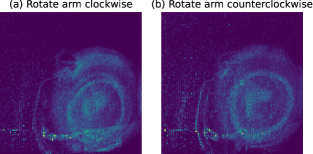
Temporal Information Elimination. In this experiment, we aim to completely remove the temporal information to observe its impact on model performance. Specifically, the entire event stream is accumulated into one frame (as depicted in Figure 13) for training a SNN. If there is a notable decline in recognition accuracy, it signifies that the temporal information holds a significant role in achieving precise recognition.

5.1.2 Comparative Datasets

We compare three of the most commonly used neuromorphic datasets in the SNN domain: DVS-Gesture (Amir et al., 2017), N-MNIST (Orchard et al., 2015), and DVS-CIFAR10 (Li et al., 2017).

DVS-Gesture comprises a series of dynamic gestures performed by 29 different individuals, spanning 11 classes, and recorded using DVS cameras under three different lighting conditions.

N-MNIST is generated by moving the ATIS vision sensor across each image in the MNIST database, encompassing all 60,000 training images and 10,000 test images.

DVS-CIFAR10 transforms the well-known CIFAR-10 dataset into a dynamic version. It contains 1000 samples for each of the 10 categories in CIFAR-10, resulting in a total of 10,000 samples.

5.1.3 Experimental Settings

All datasets were preprocessed as described in Section 4.1. The parameters $dt$ and $T$ were set to 10ms and 20, respectively. Training settings and neuron hyperparameters are comprehensively listed in Table 3, and all experiments in this study followed this configuration. Additionally, Table 4 provides the model structure parameters for each dataset.

Training Settings				Neuron Settings
Epoch	$lr$	Optimizer	$\alpha$	$V_{th}$	$V_{reset}$	$\tau$
100	0.1	Adam	2	1.0	0.0	2

Table 3: Training settings and neuron hyperparameters. $\alpha$ corresponds to the surrogate gradient parameter in equation (19), and $\tau$ represents the delay constant of the LIF neuron.

Dataset	$N_{conv}$	$N_{fc}$
N-MNIST	2	2
DVS-CIFAR10	4	2
DVS-Gesture	5	2
DVS-SLR	5	2

Table 4: Model structure parameters for different datasets. $N_{conv}$ and $N_{fc}$ are defined in Figure 7.

5.1.4 Results & Discussion

Dataset	Baseline	#Expt1	#Expt2
N-MNIST	99.21	87.71 (-11.58%)	97.72 (-1.50%)
DVS-CIFAR10	60.51	51.50 (-14.86%)	57.13 (-5.59%)
DVS-Gesture	94.78	69.07 (-27.15%)	83.14 (-12.26%)
DVS-SLR (ours)	70.49	41.54 (-41.08%)	51.46 (-26.99%)

Table 5: Comparison of recognition accuracy across different experimental conditions. The values in parentheses indicate the percentage decrease in performance compared to the baseline. #Expt1 refers to the Spike Timing Confusion experiment, while #Expt2 refers to the Temporal Information Elimination experiment.

The results presented in Table 5 clearly demonstrate that both providing the model with inaccurate temporal information (#Expt1) and retaining only the spatial information (#Expt2) lead to a reduction in recognition accuracy. This decrease is particularly significant in dynamic datasets like DVS-Gesture and our DVS-SLR, highlighting their rich temporal content. For datasets like N-MNIST and DVS-CIFAR10, which are derived from saccade transformations, completely discarding temporal information—i.e., accumulating it into a single frame—still achieves almost the same level of recognition accuracy. In these cases, the SNN is more like modeling each timestep separately and then voting on the result, which does not exploit the implicit temporal dynamics in the data. Our DVS-SLR demonstrates a more marked decline in accuracy in both experiments compared to DVS-Gesture, indicative of a stronger temporal correlation where precise spike timing is vital for accurate recognition. This can be attributed to our deliberate selection of sign language gestures, which accentuates the importance of temporal information. Additionally, the diversity in scenarios, subjects, and gestures in our DVS-SLR results in a lower baseline, offering researchers more room for improvement, as opposed to seeking marginal gains on simpler datasets.

Ultimately, our DVS-SLR is intended to serve as a benchmark dataset to encourage further research within the SNN community, particularly in exploring the spatio-temporal properties of SNNs.

5.2 Dual-modality based Recognition

5.2.1 Experimental Setup

The dual-modality data were processed into synchronized, continuous inputs $X_{event}\in{\mathbb{R}^{T\times 2\times H\times W}}$ and $X_{frame}\in{\mathbb{R}^{T\times 3\times H\times W}}$, following the method outlined in Section 4.1. The training settings and neuron hyperparameters are detailed in Table 3. During both training and inference phases, we randomly extracted segments of length $t_{lat}$ from the original data, employing these segments as inputs to our model. All experiments were replicated three times, with the mean value reported as the result.

First, we established a uni-modality baseline using the baseline model described in Section 4.2 to provide a reference point for dual-modality fusion. To thoroughly evaluate our CMA-based fusion method, we conducted extensive experiments with various fusion methods, including performance under different latency configurations and scenarios. Ablation studies were also carried out to assess the effectiveness of Temporal Attention (TA) and Spatial Attention (SA).

5.2.2 Evaluation

Latency (s)	$dt$ (ms)	$T$	Modality
			Event	Frame
0.2	10	20	70.49	64.71
	20	10	70.78	65.09
	50	4	69.05	65.14
0.5	10	50	77.78	74.71
	20	25	77.43	74.43
	50	10	77.63	75.69
1	20	50	82.32	81.71
	50	20	81.89	80.82
	100	10	82.54	80.96

Table 6: Uni-modality recognition accuracy at different latencies.

We conducted tests on the uni-modality based recognition at latencies of 0.2s, 0.5s, and 1s. The results, as shown in Table 6, reveal that the recognition accuracy is correlated with latency. As the latency increases, the classification performance for both modalities improves. This enhancement is attributed to the increased spatio-temporal information encapsulated within a longer period. At shorter latencies, the event modality exhibits markedly superior recognition accuracy compared to the frame. This superior performance is due to the higher temporal resolution of the event modality, which is adept at capturing rich motion information of the target even within brief time intervals (see Figure 8). This advantage becomes increasingly prominent as the latency decreases, showcasing the event modality’s substantial benefits in scenarios demanding rapid information processing.

Latency (s)	$dt$ (ms)	$T$	#EF	#MF	#LF		#AF	Our CMA
			Concat	Concat	OR	Average
0.2	10	20	76.54	77.43	72.92	75.83	79.67	83.67
	20	10	75.51	78.37	73.15	73.52	80.23	84.14
	50	4	77.24	77.50	72.23	74.66	80.85	82.76
0.5	10	50	77.29	78.79	76.32	75.91	80.84	83.17
	20	25	77.10	78.87	78.42	77.65	82.57	86.97
	50	10	78.62	80.67	74.22	77.43	81.45	85.46
1	20	50	79.41	79.79	78.10	80.41	82.44	85.71
	50	20	80.37	80.18	80.37	78.19	83.10	87.23
	100	10	81.41	80.16	79.86	80.11	83.21	86.39

Table 7: Comparison of fusion accuracies at different latencies. #EF denotes Early Fusion, #MF denotes Middle Fusion, #LF denotes Late Fusion, and #AF represents the attention-based fusion method proposed by (Liu et al., 2022).

As noted above, the scarcity of dual-modality datasets has limited the development of SNN-based fusion methods. The work by (Liu et al., 2022), which integrates event and neuromorphic auditory modalities, has shown impressive performance in digit recognition. Given that their fusion module’s input and output formats align with ours, we have included their algorithm in our comparative analysis. Additionally, we compared our method against other fusion methods, categorized by the timing of modality integration: early, middle, and late fusion. (i) Early Fusion (EF) is performed at the initial stages of the model, typically by concatenating the input vectors of each modality (Boulahia et al., 2021; Snoek et al., 2005). In our work, the implementation involves simply concatenating the input features $X_{e}\in\mathbb{R}^{T\times 2\times H\times W}$ and $X_{f}\in\mathbb{R}^{T\times 3\times H_{0}\times W_{0}}$ to form $X=[X_{e};X_{f}]\in\mathbb{R}^{T\times 5\times H_{0}\times W_{0}}$. (ii) Middle Fusion (MF) allows the model to independently process the information of each modality to a certain level of abstraction before fusion, which can more effectively utilize the unique attributes of each modality (Li and Wu, 2018; Nagrani et al., 2021). Here, we concatenate the outputs of the SpikingConv Encoder for each modality, $s^{n}=[s_{e}^{n};s_{f}^{n}]\in\mathbb{R}^{T\times 2C\times H_{n}\times W_{n}}$, and subsequently input this combined data into the SpikingFC Decoder. (iii) Late Fusion (LF) occurs at the decision-making layer (Gadzicki et al., 2020). We employed two fusion approaches: performing an element-wise OR operation on the output spikes from each modality, and averaging the predicted probabilities.

Figure 14: Test accuracy curves under various latency configurations. Here, $dt$ is fixed at 20$ms$. Each graph incorporates three curves, respectively representing frame based and event based uni-modality recognition, along with our CMA fusion.

As illustrated in Figure 14, across all latency parameters, the incorporation of the CMA module consistently enhances recognition accuracy compared to uni-modality recognition, with this improvement being particularly pronounced at lower latency settings. This is attributable to the frame modality’s inability to provide sufficient dynamic information at such settings. In contrast, the CMA module effectively bridges the dynamic features from the event modality with the static attributes captured in the frame modality, thereby enriching the model’s analytical depth and precision. The results of the dual-modality comparison experiments are presented in Table 7. It is evident that the attention-based fusion (AF) method, as proposed in (Liu et al., 2022), demonstrates superior performance over other simpler fusion approaches. This method simply computes attention scores for the spatio-temporal features of each modality, without adequately adapting to the unique characteristics inherent to each type of data. Our approach, on the other hand, employs Temporal-wise Attention (TA) and Spatial-wise Attention (SA) specifically for the event and frame modalities, respectively, thus more effectively leveraging the strengths of each modality, and consequently achieving optimal performance.

5.2.3 Scenario Study

Controlled Scenario		Modality		Our CMA
		Event	Frame
Light	dimLED	76.29	66.75	81.56
	brightLED	79.29	77.53	83.41
	naturalLight	77.05	78.64	82.07
Position	back	74.28	75.02	83.77
	front	82.59	80.51	84.49

Table 8: Recognition accuracy of event and frame streams under various lighting conditions and positions. $dt$ and $T$ are set to 50$ms$ and 20, respectively.

Our dataset encompasses three distinct lighting conditions and two different positions. To analyze the unique characteristics of each modality and to verify the effectiveness of our fusion method, we extracted subsets from the full dataset for training and evaluation. The experimental results, as presented in Table 8, highlight several key findings: (i) Superior Performance of Event Modality in Low-Light Conditions. In low-light scenarios, the baseline model demonstrates a substantial decrease in recognition accuracy for the frame modality, while the event modality maintains a relatively high level of accuracy. This can be attributed to the unique generation mechanism of events. Unlike traditional RGB cameras that capture static light intensity information, event cameras only record changes in light intensity. Consequently, they have a higher dynamic range and are capable of accurately capturing and representing dynamic changes within scenes even under low-light conditions, thereby ensuring higher recognition accuracy. (ii) The Influence of Position on Recognition Accuracy. Datasets labeled as ’front’ show enhanced recognition accuracy compared to those marked as ’back’. This difference is likely due to the superior signal-to-noise ratio found in the ’front’ datasets. (iii) Enhanced Model Robustness Through CMA Integration. The incorporation of the CMA module has significantly improved accuracy across all scenarios, particularly notable in low-light conditions where the frame modality initially underperformed. Furthermore, the integration of the CMA module has led to a marked reduction in the discrepancy in accuracy across different conditions, indicating that the model has become less sensitive to varying scenarios and has achieved greater robustness.

5.2.4 Ablation Study

Modality		Acc
Event	Frame
TA	SA	87.23
TA	TA	86.17
SA	SA	85.71
SA	TA	85.42

Table 9: Recognition accuracy comparison with different attention score generation strategies for each modality ($dt=50ms$, $T=20$)

Impact of attention score generation strategy. The CMA module functions by independently extracting temporal attention scores using temporal-wise attention (TA) and spatial attention scores using spatial-wise attention (SA), followed by their cross-fusion to produce enhanced features. We evaluated the effectiveness of this attention generation strategy. As shown in Table 9, the recognition accuracy was compared when applying different attention generation strategies to each modality. The results indicate that our method surpasses others in terms of accuracy, highlighting that such a combination more effectively utilizes the distinct characteristics inherent to each modality.

Figure 15: The relationship between different placement positions of the CMA module and accuracy. $dt$ is set to 50ms. S1: $T=4$, S2: $T=10$, S3: $T=20$.

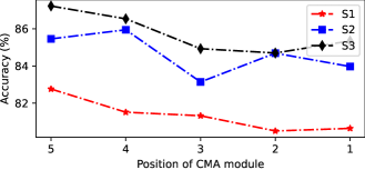
Impact of CMA module placement. In our previous experiments, the CMA module was placed following the last convolutional block, setting $n$ equal to $N_{conv}=5$. However, the placement of the CMA module within the network can influence its performance. As evident from Figure 15, placing the CMA module in deeper layers slightly outperforms its placement in shallower layers. This finding aligns with observations in (Yao et al., 2021; Hu et al., 2018), where attention modules applied to deep features also exhibited enhanced performance. Our experimental results show the effectiveness of fusion module placement.

Effectiveness of CMA module on different spiking neurons. All experiments in this paper use the Leaky Integrate-and-Fire (LIF) neuron model. In this section, we discuss the performance of the CMA model on different neurons. We have selected the Integrate and Fire (IF), Parametric LIF (PLIF) (Fang et al., 2021), and Leaky Integrate and Analog Fire (LIAF) (Wu et al., 2021) neurons for evaluation. The IF neuron is a simplification of LIF, omitting the "leaky" process, meaning the time constant $\tau$ is taken to be infinite. PLIF operates under the same computational paradigm as LIF, but with a trainable $\tau$. LIAF updates the membrane potential in the same way as LIF, but uses an analog activation for output. Following (Wu et al., 2021), the scaled exponential linear unit (SELU) is applied as the activation function here. Table 10 shows the recognition accuracies of these neurons using our CMA fusion and simple middle feature concat fusion respectively. It can be observed that without CMA, PLIF and LIAF achieve higher accuracies than LIF due to their more complex spatio-temporal representation. The CMA method enhances performance across all neuron types, but the improvement is smaller for LIAF. This may be due to the LIAF model using an analog activation for information transmission, while our CMA module is designed for spike-based outputs.

$dt$ (ms)	$T$	Model Performance (With/Without CMA)
		LIF		IF		PLIF		LIAF
20	10	84.14	78.37	82.78	77.21	85.33	79.70	83.27	80.05
	25	86.97	78.87	84.01	77.53	86.74	79.63	84.10	81.73
	50	85.71	79.79	85.12	78.40	86.97	80.91	84.54	81.91

Table 10: Recognition accuracies of different spiking neuron models with and without CMA fusion.

6 Conclusion

In this work, we firstly verified the inadequacy of current neuromorphic datasets in terms of temporal correlation through Spike Timing Confusion and Temporal Information Elimination experiments. Addressing this, we designed and recorded the DVS-SLR dataset which exhibits high temporal correlation and effectively exploits the spatio-temporal processing capabilities of SNNs. Additionally, our neuromorphic dataset includes corresponding frame data, making it a valuable resource for developing SNN-based fusion techniques.

Secondly, we propose a Cross-Modality Attention (CMA)-based fusion approach. The CMA module efficiently utilizes the unique advantages of each modality, which enables SNNs to learn both temporal and spatial attention scores from the spatio-temporal features of event and frame modalities. Experimental results demonstrate that our method not only improves recognition accuracy but also ensures robustness across diverse scenarios.

References

- He et al. (2020) W. He, Y. Wu, L. Deng, G. Li, H. Wang, Y. Tian, W. Ding, W. Wang, Y. Xie, Comparing snns and rnns on neuromorphic vision datasets: Similarities and differences, Neural Networks 132 (2020) 108–120. URL: https://www.sciencedirect.com/science/article/pii/S0893608020302902. doi:https://doi.org/10.1016/j.neunet.2020.08.001.
- Iyer et al. (2021) L. R. Iyer, Y. Chua, H. Li, Is neuromorphic mnist neuromorphic? analyzing the discriminative power of neuromorphic datasets in the time domain, Frontiers in Neuroscience 15 (2021). URL: https://www.frontiersin.org/articles/10.3389/fnins.2021.608567. doi:10.3389/fnins.2021.608567.
- Deng et al. (2020) L. Deng, Y. Wu, X. Hu, L. Liang, Y. Ding, G. Li, G. Zhao, P. Li, Y. Xie, Rethinking the performance comparison between snns and anns, Neural networks 121 (2020) 294–307.
- Li et al. (2022) Y. Li, Y. Dong, D. Zhao, Y. Zeng, N-omniglot, a large-scale neuromorphic dataset for spatio-temporal sparse few-shot learning, Scientific Data 9 (2022) 746.
- Luo et al. (2022) Y. Luo, H. Shen, X. Cao, T. Wang, Q. Feng, Z. Tan, Conversion of siamese networks to spiking neural networks for energy-efficient object tracking, Neural Computing and Applications 34 (2022) 9967–9982.
- Wang et al. (2021) X. Wang, J. Li, L. Zhu, Z. Zhang, Z. Chen, X. Li, Y. Wang, Y. Tian, F. Wu, Visevent: Reliable object tracking via collaboration of frame and event flows, arXiv preprint arXiv:2108.05015 (2021).
- Paikin et al. (2021) G. Paikin, Y. Ater, R. Shaul, E. Soloveichik, Efi-net: Video frame interpolation from fusion of events and frames, in: Proceedings of the IEEE/CVF Conference on Computer Vision and Pattern Recognition, 2021, pp. 1291–1301.
- Tulyakov et al. (2022) S. Tulyakov, A. Bochicchio, D. Gehrig, S. Georgoulis, Y. Li, D. Scaramuzza, Time lens++: Event-based frame interpolation with parametric non-linear flow and multi-scale fusion, in: Proceedings of the IEEE/CVF Conference on Computer Vision and Pattern Recognition, 2022, pp. 17755–17764.
- Weikersdorfer et al. (2014) D. Weikersdorfer, D. B. Adrian, D. Cremers, J. Conradt, Event-based 3d slam with a depth-augmented dynamic vision sensor, in: 2014 IEEE international conference on robotics and automation (ICRA), IEEE, 2014, pp. 359–364.
- Cheng et al. (2022) J. Cheng, L. Zhang, Q. Chen, X. Hu, J. Cai, A review of visual slam methods for autonomous driving vehicles, Engineering Applications of Artificial Intelligence 114 (2022) 104992.
- Gerstner et al. (2014) W. Gerstner, W. M. Kistler, R. Naud, L. Paninski, Neuronal dynamics: From single neurons to networks and models of cognition, Cambridge University Press, 2014.
- Bouvier et al. (2019) M. Bouvier, A. Valentian, T. Mesquida, F. Rummens, M. Reyboz, E. Vianello, E. Beigne, Spiking neural networks hardware implementations and challenges: A survey, ACM Journal on Emerging Technologies in Computing Systems (JETC) 15 (2019) 1–35.
- Diehl et al. (2015) P. U. Diehl, D. Neil, J. Binas, M. Cook, S.-C. Liu, M. Pfeiffer, Fast-classifying, high-accuracy spiking deep networks through weight and threshold balancing, in: 2015 International joint conference on neural networks (IJCNN), ieee, 2015, pp. 1–8.
- Diehl et al. (2016) P. U. Diehl, G. Zarrella, A. Cassidy, B. U. Pedroni, E. Neftci, Conversion of artificial recurrent neural networks to spiking neural networks for low-power neuromorphic hardware, in: 2016 IEEE International Conference on Rebooting Computing (ICRC), IEEE, 2016, pp. 1–8.
- Han et al. (2023) J. Han, Z. Wang, J. Shen, H. Tang, Symmetric-threshold relu for fast and nearly lossless ann-snn conversion, Machine Intelligence Research 20 (2023) 435–446.
- Qu et al. (2024) J. Qu, Z. Gao, T. Zhang, Y. Lu, H. Tang, H. Qiao, Spiking neural network for ultralow-latency and high-accurate object detection, IEEE Transactions on Neural Networks and Learning Systems (2024) 1–13. doi:10.1109/TNNLS.2024.3372613.
- Zhang et al. (2023) A. Zhang, J. Shi, J. Wu, Y. Zhou, W. Yu, Low latency and sparse computing spiking neural networks with self-driven adaptive threshold plasticity, IEEE Transactions on Neural Networks and Learning Systems (2023).
- Zhang et al. (2021) A. Zhang, X. Li, Y. Gao, Y. Niu, Event-driven intrinsic plasticity for spiking convolutional neural networks, IEEE Transactions on Neural Networks and Learning Systems 33 (2021) 1986–1995.
- Fang et al. (2021) W. Fang, Z. Yu, Y. Chen, T. Huang, T. Masquelier, Y. Tian, Deep residual learning in spiking neural networks, in: M. Ranzato, A. Beygelzimer, Y. Dauphin, P. Liang, J. W. Vaughan (Eds.), Advances in Neural Information Processing Systems, volume 34, Curran Associates, Inc., 2021, pp. 21056–21069. URL: https://proceedings.neurips.cc/paper_files/paper/2021/file/afe434653a898da20044041262b3ac74-Paper.pdf.
- Bu et al. (2023) T. Bu, W. Fang, J. Ding, P. Dai, Z. Yu, T. Huang, Optimal ann-snn conversion for high-accuracy and ultra-low-latency spiking neural networks, arXiv preprint arXiv:2303.04347 (2023).
- Hao et al. (2023) Z. Hao, T. Bu, J. Ding, T. Huang, Z. Yu, Reducing ann-snn conversion error through residual membrane potential, arXiv preprint arXiv:2302.02091 (2023).
- Rueckauer et al. (2017) B. Rueckauer, I.-A. Lungu, Y. Hu, M. Pfeiffer, S.-C. Liu, Conversion of continuous-valued deep networks to efficient event-driven networks for image classification, Frontiers in neuroscience 11 (2017) 682.
- Wang et al. (2023) Z. Wang, Y. Zhang, S. Lian, X. Cui, R. Yan, H. Tang, Toward high-accuracy and low-latency spiking neural networks with two-stage optimization, IEEE Transactions on Neural Networks and Learning Systems (2023).
- Wu et al. (2019) Y. Wu, L. Deng, G. Li, J. Zhu, Y. Xie, L. Shi, Direct training for spiking neural networks: Faster, larger, better, in: Proceedings of the AAAI conference on artificial intelligence, volume 33, 2019, pp. 1311–1318.
- Werbos (1990) P. J. Werbos, Backpropagation through time: what it does and how to do it, Proceedings of the IEEE 78 (1990) 1550–1560.
- Fang et al. (2021) W. Fang, Z. Yu, Y. Chen, T. Masquelier, T. Huang, Y. Tian, Incorporating learnable membrane time constant to enhance learning of spiking neural networks, in: Proceedings of the IEEE/CVF international conference on computer vision, 2021, pp. 2661–2671.
- Yu et al. (2022) Q. Yu, J. Gao, J. Wei, J. Li, K. C. Tan, T. Huang, Improving multispike learning with plastic synaptic delays, IEEE Transactions on Neural Networks and Learning Systems (2022).
- Ma et al. (2023) G. Ma, R. Yan, H. Tang, Exploiting noise as a resource for computation and learning in spiking neural networks, Patterns (2023). doi:10.1016/j.patter.2023.100831.
- Hu et al. (2021) Y. Hu, H. Tang, G. Pan, Spiking deep residual networks, IEEE Transactions on Neural Networks and Learning Systems (2021).
- Fang et al. (2021) W. Fang, Z. Yu, Y. Chen, T. Huang, T. Masquelier, Y. Tian, Deep residual learning in spiking neural networks, Advances in Neural Information Processing Systems 34 (2021) 21056–21069.
- Yao et al. (2021) M. Yao, H. Gao, G. Zhao, D. Wang, Y. Lin, Z. Yang, G. Li, Temporal-wise attention spiking neural networks for event streams classification, in: Proceedings of the IEEE/CVF International Conference on Computer Vision, 2021, pp. 10221–10230.
- Feng et al. (2022) L. Feng, Q. Liu, H. Tang, D. Ma, G. Pan, Multi-level firing with spiking ds-resnet: Enabling better and deeper directly-trained spiking neural networks, arXiv preprint arXiv:2210.06386 (2022).
- Xie et al. (2023) X. Xie, Y. Chua, G. Liu, M. Zhang, G. Luo, H. Tang, Event-driven spiking learning algorithm using aggregated labels, IEEE Transactions on Neural Networks and Learning Systems (2023).
- Zheng et al. (2021) H. Zheng, Y. Wu, L. Deng, Y. Hu, G. Li, Going deeper with directly-trained larger spiking neural networks, in: Proceedings of the AAAI conference on artificial intelligence, volume 35, 2021, pp. 11062–11070.
- Yang et al. (2022) Q. Yang, J. Wu, M. Zhang, Y. Chua, X. Wang, H. Li, Training spiking neural networks with local tandem learning, Advances in Neural Information Processing Systems 35 (2022) 12662–12676.
- Wang et al. (2023) Z. Wang, R. Jiang, S. Lian, R. Yan, H. Tang, Adaptive smoothing gradient learning for spiking neural networks, in: International Conference on Machine Learning, PMLR, 2023, pp. 35798–35816.
- Gu et al. (2019) P. Gu, R. Xiao, G. Pan, H. Tang, Stca: Spatio-temporal credit assignment with delayed feedback in deep spiking neural networks., in: IJCAI, volume 15, 2019, pp. 1366–1372.
- Liu et al. (2021) Q. Liu, D. Xing, H. Tang, D. Ma, G. Pan, Event-based action recognition using motion information and spiking neural networks., in: IJCAI, 2021, pp. 1743–1749.
- Gao et al. (2023) Y. Gao, J. Lu, S. Li, N. Ma, S. Du, Y. Li, Q. Dai, Action recognition and benchmark using event cameras, IEEE Transactions on Pattern Analysis and Machine Intelligence (2023).
- Cao et al. (2015) Z. Cao, L. Cheng, C. Zhou, N. Gu, X. Wang, M. Tan, Spiking neural network-based target tracking control for autonomous mobile robots, Neural Computing and Applications 26 (2015) 1839–1847.
- Yang et al. (2023) B. Yang, M. Yuan, C. Zhang, C. Hong, G. Pan, H. Tang, Spiking reinforcement learning with memory ability for mapless navigation, in: 2023 IEEE/RSJ International Conference on Intelligent Robots and Systems (IROS), IEEE, 2023, pp. 1–8.
- Debat et al. (2021) G. Debat, T. Chauhan, B. R. Cottereau, T. Masquelier, M. Paindavoine, R. Baures, Event-based trajectory prediction using spiking neural networks, Frontiers in computational neuroscience 15 (2021) 658764.
- Yu et al. (2024) L. Yu, H. Chen, Z. Wang, S. Zhan, J. Shao, Q. Liu, S. Xu, Spikingvit: a multi-scale spiking vision transformer model for event-based object detection, IEEE Transactions on Cognitive and Developmental Systems (2024).
- Yuan et al. (2024) M. Yuan, C. Zhang, Z. Wang, H. Liu, G. Pan, H. Tang, Trainable spiking-yolo for low-latency and high-performance object detection, Neural Networks 172 (2024) 106092.
- Anumula et al. (2018) J. Anumula, D. Neil, T. Delbruck, S.-C. Liu, Feature representations for neuromorphic audio spike streams, Frontiers in neuroscience 12 (2018) 23.
- See et al. (2020) H. H. See, B. Lim, S. Li, H. Yao, W. Cheng, H. Soh, B. C. Tee, St-mnist–the spiking tactile mnist neuromorphic dataset, arXiv preprint arXiv:2005.04319 (2020).
- Vanarse et al. (2022) A. Vanarse, A. Osseiran, A. Rassau, P. van der Made, Application of neuromorphic olfactory approach for high-accuracy classification of malts, Sensors 22 (2022) 440.
- Rebecq et al. (2018) H. Rebecq, D. Gehrig, D. Scaramuzza, Esim: an open event camera simulator, in: Conference on robot learning, PMLR, 2018, pp. 969–982.
- Hu et al. (2021) Y. Hu, S.-C. Liu, T. Delbruck, v2e: From video frames to realistic dvs events, in: Proceedings of the IEEE/CVF Conference on Computer Vision and Pattern Recognition, 2021, pp. 1312–1321.
- Zhang et al. (2023) J. Zhang, Y. Wang, W. Liu, M. Li, J. Bai, B. Yin, X. Yang, Frame-event alignment and fusion network for high frame rate tracking, in: Proceedings of the IEEE/CVF Conference on Computer Vision and Pattern Recognition, 2023, pp. 9781–9790.
- Gehrig et al. (2021) D. Gehrig, M. Rüegg, M. Gehrig, J. Hidalgo-Carrió, D. Scaramuzza, Combining events and frames using recurrent asynchronous multimodal networks for monocular depth prediction, IEEE Robotics and Automation Letters 6 (2021) 2822–2829.
- Li et al. (2023) Y. Li, Z. Huang, S. Chen, X. Shi, H. Li, H. Bao, Z. Cui, G. Zhang, Blinkflow: A dataset to push the limits of event-based optical flow estimation, arXiv preprint arXiv:2303.07716 (2023).
- Wang et al. (2019) L. Wang, Y.-S. Ho, K.-J. Yoon, et al., Event-based high dynamic range image and very high frame rate video generation using conditional generative adversarial networks, in: Proceedings of the IEEE/CVF Conference on Computer Vision and Pattern Recognition, 2019, pp. 10081–10090.
- Orchard et al. (2015) G. Orchard, A. Jayawant, G. K. Cohen, N. Thakor, Converting static image datasets to spiking neuromorphic datasets using saccades, Frontiers in neuroscience 9 (2015) 437.
- Kim et al. (2021) J. Kim, J. Bae, G. Park, D. Zhang, Y. M. Kim, N-imagenet: Towards robust, fine-grained object recognition with event cameras, in: Proceedings of the IEEE/CVF International Conference on Computer Vision, 2021, pp. 2146–2156.
- Li et al. (2017) H. Li, H. Liu, X. Ji, G. Li, L. Shi, Cifar10-dvs: an event-stream dataset for object classification, Frontiers in neuroscience 11 (2017) 309.
- Lin et al. (2021) Y. Lin, W. Ding, S. Qiang, L. Deng, G. Li, Es-imagenet: A million event-stream classification dataset for spiking neural networks, Frontiers in Neuroscience 15 (2021). URL: https://www.frontiersin.org/articles/10.3389/fnins.2021.726582. doi:10.3389/fnins.2021.726582.
- Hu et al. (2016) Y. Hu, H. Liu, M. Pfeiffer, T. Delbruck, Dvs benchmark datasets for object tracking, action recognition, and object recognition, Frontiers in neuroscience 10 (2016) 405.
- Amir et al. (2017) A. Amir, B. Taba, D. Berg, T. Melano, J. McKinstry, C. Di Nolfo, T. Nayak, A. Andreopoulos, G. Garreau, M. Mendoza, et al., A low power, fully event-based gesture recognition system, in: Proceedings of the IEEE conference on computer vision and pattern recognition, 2017, pp. 7243–7252.
- Vasudevan et al. (2021) A. Vasudevan, P. Negri, C. Di Ielsi, B. Linares-Barranco, T. Serrano-Gotarredona, Sl-animals-dvs: event-driven sign language animals dataset, Pattern Analysis and Applications (2021) 1–16.
- Miao et al. (2019) S. Miao, G. Chen, X. Ning, Y. Zi, K. Ren, Z. Bing, A. Knoll, Neuromorphic vision datasets for pedestrian detection, action recognition, and fall detection, Frontiers in Neurorobotics 13 (2019). URL: https://www.frontiersin.org/articles/10.3389/fnbot.2019.00038. doi:10.3389/fnbot.2019.00038.
- Dong et al. (2022) J. Dong, R. Jiang, R. Xiao, R. Yan, H. Tang, Event stream learning using spatio-temporal event surface, Neural Networks 154 (2022) 543–559.
- Serrano-Gotarredona and Linares-Barranco (2015) T. Serrano-Gotarredona, B. Linares-Barranco, Poker-dvs and mnist-dvs. their history, how they were made, and other details, Frontiers in neuroscience 9 (2015) 481.
- Sironi et al. (2018) A. Sironi, M. Brambilla, N. Bourdis, X. Lagorce, R. Benosman, Hats: Histograms of averaged time surfaces for robust event-based object classification, in: Proceedings of the IEEE conference on computer vision and pattern recognition, 2018, pp. 1731–1740.
- Leow and Nikolic (2015) H. Leow, K. Nikolic, Machine vision using combined frame-based and event-based vision sensor, in: 2015 IEEE International Symposium on Circuits and Systems (ISCAS), IEEE, 2015, pp. 706–709.
- Lele et al. (2022) A. S. Lele, Y. Fang, A. Anwar, A. Raychowdhury, Bio-mimetic high-speed target localization with fused frame and event vision for edge application, Frontiers in Neuroscience 16 (2022) 1010302.
- Natan and Miura (2021) O. Natan, J. Miura, Semantic segmentation and depth estimation with rgb and dvs sensor fusion for multi-view driving perception, in: Asian Conference on Pattern Recognition, Springer, 2021, pp. 352–365.
- Bi et al. (2023) X. Bi, M. Li, F. Zha, W. Guo, P. Wang, A non-uniform illumination image enhancement method based on fusion of events and frames, Optik 272 (2023) 170329.
- Lichtsteiner et al. (2008) P. Lichtsteiner, C. Posch, T. Delbruck, A s latency asynchronous temporal contrast vision sensor, IEEE journal of solid-state circuits 43 (2008) 566–576.
- Posch et al. (2010) C. Posch, D. Matolin, R. Wohlgenannt, A qvga 143 db dynamic range frame-free pwm image sensor with lossless pixel-level video compression and time-domain cds, IEEE Journal of Solid-State Circuits 46 (2010) 259–275.
- Inivation (2019) Inivation, Davis346 datasheet, https://inivation.com/wp-content/uploads/2019/08/DAVIS346.pdf, 2019. Accessed on: 2023-09-19.
- Simonyan and Zisserman (2014) K. Simonyan, A. Zisserman, Two-stream convolutional networks for action recognition in videos, Advances in neural information processing systems 27 (2014).
- Carreira and Zisserman (2017) J. Carreira, A. Zisserman, Quo vadis, action recognition? a new model and the kinetics dataset, in: proceedings of the IEEE Conference on Computer Vision and Pattern Recognition, 2017, pp. 6299–6308.
- Feichtenhofer et al. (2019) C. Feichtenhofer, H. Fan, J. Malik, K. He, Slowfast networks for video recognition, in: Proceedings of the IEEE/CVF international conference on computer vision, 2019, pp. 6202–6211.
- Woo et al. (2018) S. Woo, J. Park, J.-Y. Lee, I. S. Kweon, Cbam: Convolutional block attention module, in: Proceedings of the European conference on computer vision (ECCV), 2018, pp. 3–19.
- Yao et al. (2023) M. Yao, G. Zhao, H. Zhang, Y. Hu, L. Deng, Y. Tian, B. Xu, G. Li, Attention spiking neural networks, IEEE transactions on pattern analysis and machine intelligence (2023).
- Salinas and Sejnowski (2000) E. Salinas, T. J. Sejnowski, Impact of correlated synaptic input on output firing rate and variability in simple neuronal models, Journal of neuroscience 20 (2000) 6193–6209.
- Zhang and Li (2020) W. Zhang, P. Li, Temporal spike sequence learning via backpropagation for deep spiking neural networks, Advances in Neural Information Processing Systems 33 (2020) 12022–12033.
- Yang et al. (2021) Y. Yang, W. Zhang, P. Li, Backpropagated neighborhood aggregation for accurate training of spiking neural networks, in: International Conference on Machine Learning, PMLR, 2021, pp. 11852–11862.
- Hong et al. (2024) C. Hong, M. Yuan, M. Zhang, X. Wang, C. Zhang, J. Wang, G. Pan, H. Tang, Spaic: a spike-based artificial intelligence computing framework, IEEE Computational Intelligence Magazine 19 (2024) 51–65.
- Fang et al. (2023) W. Fang, Y. Chen, J. Ding, Z. Yu, T. Masquelier, D. Chen, L. Huang, H. Zhou, G. Li, Y. Tian, Spikingjelly: An open-source machine learning infrastructure platform for spike-based intelligence, Science Advances 9 (2023) eadi1480.
- Liu et al. (2022) Q. Liu, D. Xing, L. Feng, H. Tang, G. Pan, Event-based multimodal spiking neural network with attention mechanism, in: ICASSP 2022-2022 IEEE International Conference on Acoustics, Speech and Signal Processing (ICASSP), IEEE, 2022, pp. 8922–8926.
- Boulahia et al. (2021) S. Y. Boulahia, A. Amamra, M. R. Madi, S. Daikh, Early, intermediate and late fusion strategies for robust deep learning-based multimodal action recognition, Machine Vision and Applications 32 (2021) 121.
- Snoek et al. (2005) C. G. Snoek, M. Worring, A. W. Smeulders, Early versus late fusion in semantic video analysis, in: Proceedings of the 13th annual ACM international conference on Multimedia, 2005, pp. 399–402.
- Li and Wu (2018) H. Li, X.-J. Wu, Densefuse: A fusion approach to infrared and visible images, IEEE Transactions on Image Processing 28 (2018) 2614–2623.
- Nagrani et al. (2021) A. Nagrani, S. Yang, A. Arnab, A. Jansen, C. Schmid, C. Sun, Attention bottlenecks for multimodal fusion, Advances in neural information processing systems 34 (2021) 14200–14213.
- Gadzicki et al. (2020) K. Gadzicki, R. Khamsehashari, C. Zetzsche, Early vs late fusion in multimodal convolutional neural networks, in: 2020 IEEE 23rd international conference on information fusion (FUSION), IEEE, 2020, pp. 1–6.
- Hu et al. (2018) J. Hu, L. Shen, G. Sun, Squeeze-and-excitation networks, in: 2018 IEEE/CVF Conference on Computer Vision and Pattern Recognition, 2018, pp. 7132–7141. doi:10.1109/CVPR.2018.00745.
- Wu et al. (2021) Z. Wu, H. Zhang, Y. Lin, G. Li, M. Wang, Y. Tang, Liaf-net: Leaky integrate and analog fire network for lightweight and efficient spatiotemporal information processing, IEEE Transactions on Neural Networks and Learning Systems 33 (2021) 6249–6262.