RANSAC Back to SOTA: A Two-stage Consensus Filtering for Real-time 3D Registration
Abstract
Correspondence-based point cloud registration (PCR) plays a key role in robotics and computer vision. However, challenges like sensor noises, object occlusions, and descriptor limitations inevitably result in numerous outliers. RANSAC family is the most popular outlier removal solution. However, the requisite iterations escalate exponentially with the outlier ratio, rendering it far inferior to existing methods (SC2PCR[1], MAC[2], etc.) in terms of accuracy or speed. Thus, we propose a two-stage consensus filtering (TCF) that elevates RANSAC to state-of-the-art (SOTA) speed and accuracy. Firstly, one-point RANSAC obtains a consensus set based on length consistency. Subsequently, two-point RANSAC refines the set via angle consistency. Then, three-point RANSAC computes a coarse pose and removes outliers based on transformed correspondence’s distances. Drawing on optimizations from one-point and two-point RANSAC, three-point RANSAC requires only a few iterations. Eventually, an iterative reweighted least squares (IRLS) is applied to yield the optimal pose. Experiments on the large-scale KITTI and ETH datasets demonstrate our method achieves up to three-orders-of-magnitude speedup compared to MAC while maintaining registration accuracy and recall. Our code is available at https://github.com/ShiPC-AI/TCF.
Index Terms:
Point cloud registration, correspondence, consensus filtering, RANSAC, iteratively reweighted least squares.I Introduction
Point cloud registration (PCR) seeks to estimate a six-degree-of-freedom (6-DOF) pose to align point clouds, which is crucial for 3D reconstruction[3, 4, 5, 6], robotic navigation[7, 8, 9, 10], and aerial photogrammetry[11, 12, 13, 14]. Iterative closest point (ICP)[15] pioneers a local registration pipeline that iteratively searches correspondences and minimizes their distances. Unfortunately, it often converges to erroneous local optima under notable viewpoint changes[16, 17, 18]. To overcome this, researchers derive coarse poses from feature correspondences[19, 20], known as correspondence-based PCR. However, sensor noises, object occlusions, and descriptor limitations inevitably lead to outliers, presenting great challenges for registration[21, 22, 23].
Random sample consensus (RANSAC) [24, 25, 26, 27, 28] is the most popular solution to handle correspondences with outliers. It follows a generation-and-selection strategy that iteratively samples correspondences to generate and verify hypotheses. However, the requisite iterations escalate exponentially with the outlier ratio, which renders them far inferior to existing methods in accuracy and efficiency.
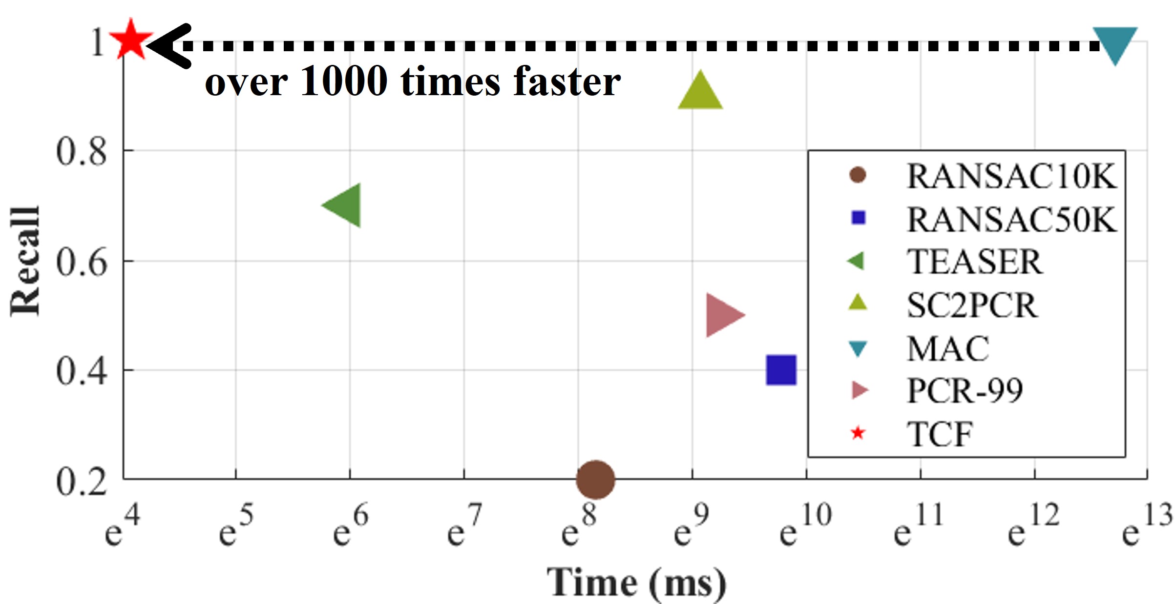
Thus, we propose a two-stage consensus filtering (TCF) incorporating one-point and two-point RANSAC steps before the three-point RANSAC to ensure accuracy and significantly boost efficiency. It begins with a one-point RANSAC to remove correspondence outliers via length constraints. Afterward, a two-point RANSAC evaluates the angle consistency to get a more reliable consensus. This design significantly reduces the iteration number by lowering the sampling dimension and also decreases the outlier ratio. As a result, the three-point RANSAC requires only a few iterations, enhancing registration performance. Following this, three-point RANSAC computes a coarse pose and removes outliers based on transformed correspondence’s distances. Finally, a scale-adaptive Cauchy iteratively reweighted least squares (IRLS) is applied to calculate the optimal pose. As depicted in Fig. 1, our method demonstrates SOTA performance and achieves a speedup of up to three orders of magnitude.
The main contributions are as follows:
-
•
We devise a two-stage filtering method that swiftly eliminates the majority of correspondence outliers, facilitating RANSAC to reach SOTA levels.
-
•
Based on our filtering method, we formulate a complete PCR pipeline. On large-scale outdoor datasets, it markedly enhances efficiency while ensuring accuracy.
II Related Work
II-A Handcrafted PCR
RANSAC Family. This type of method follows a generation-and-selection strategy. GC-RANSAC[28] devises a locally optimized pipeline alternating between graph cut and model re-fitting. CG-SAC[20] evaluates correspondence compatibility by calculating distances between salient points and employs a compatibility-guided strategy to reduce sampling randomness. SC2-PCR[1] evaluates correspondence similarity using second-order spatial compatibility, applies a global spectral technique to identify reliable seeds, and uses a two-stage approach to expand each seed into a consensus set. To expedite processing, PCR-99[29] devises an improved sample ordering guided by pairwise scale consistency and a triplet scale consistency-based outlier rejection scheme. Their performance depends on model parameter selection and requires tuning for specific problems. Runtime increases exponentially with large-scale data, especially when the outliers prevail.
Graph Theory. These methods model the correspondence set as a graph and use graph theories to achieve robust registration. MAC [2] loosens the maximum clique constraint to mine more local consensus information from a graph. It identifies maximal cliques and performs node-guided selection based on the clique with the highest graph weight. CLIPPER [30] ensures dense subgraph solutions with continuous relaxation and achieves efficiency using projected gradient ascent and backtracking line search. ROBIN [31] checks the compatibility of measurement subsets using invariants and prunes outliers by finding the maximum clique or k-core in the graph induced. TEASER [19] reformulates the registration problem using a truncated least squares (TLS) cost and introduces a graph-theoretic framework to decouple and sequentially solve scale, rotation, and translation estimation. Graph-based methods effectively leverage topology information and handle complex scenes but struggle with high algorithmic complexity.
Loss Optimization. This category of methods progressively optimizes error functions to refine the pose. Iterative closest point (ICP)[15] pioneers a local registration pipeline that iteratively searches correspondences and minimizes Euclidean distances. Following this, several works seek to advance ICP from diverse perspectives, such as incorporating the point-to-plane metric[32], probabilistic models[33], and branch-and-bound (BnB) theories[34]. Despite robust results, poor initial guess tends to yield wrong results. Fast global registration (FGR)[4] formulates a dense objective featuring a scaled Geman-McClure estimator as the penalty function and alleviates the impact of local minima via graduated non-convexity. Yang et al. [35] propose a versatile approach for robust estimation that utilizes modern non-minimal solvers, extending the applicability of Black-Rangarajan duality and graduated non-convexity (GNC) to various spatial perception tasks, including mesh registration, shape alignment, and pose graph optimization.
II-B Learning-based PCR
End-to-end Direct Registration. End-to-end methods optimize all steps within a unified framework, directly producing registration results through the network. Deep Closest Point (DCP)[22] employs DGCNN[36] for correspondence identification and a pointer network [37] for soft matching, estimates the rigid transformation with a differentiable single value decomposition (SVD) layer. However, it struggles with partially overlapping point clouds. REGTR[11] employs a transformer network to estimate the probability of each point residing in the overlapping region, thereby supplanting explicit feature matching and RANSAC[24]. CCAG[5] employs cross-attention mechanisms and depth-wise separable convolutions to capture point cloud relationships. Additionally, it introduces an adaptive graph convolution multi-layer perceptron (MLP) to augment node expressiveness. Although proficient with synthetic datasets, these methods may falter on real-world data, limiting their accuracy and practical utility.
Descriptor Learning. Descriptor learning mainly aims to create sparse descriptions for local 3D patches using a weight-sharing network or produce dense descriptions for the entire point cloud in a single forward pass. The pioneering work 3DMatch[3] converts local 3D patches into volumetric representations and then derives descriptors via a siamese convolutional network. FCGF[38] adopts sparse tensor representation and employs Minkowski convolutional neural networks as the backbone to learn dense features. Several works successively boost the feature descriptiveness via N-tuple loss[39], folding-based encoder[40], and spherical CNNs[41]. Predator[21] adds an overlap-attention block to aggregate contextual information for robust registration in low-overlap scenarios. While they eliminate manual feature design and bolster robustness, substantial labeling, training, and optimization remain time-consuming, particularly for low-cost robot platforms.
III Method
III-A Motivation
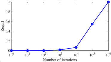
The minimum iteration, , required by RANSAC is computed as:
| (1) |
where is the outlier ratio. denotes the sample size. is a ceiling function. represents the probability of at least one perfect minimal subset, preset to a default value of 0.99. As shown in Fig. 2, we evaluate the registration recall of 200 pairs of point clouds at different iterations. As iterations increase from to and , registration recall improves from 2% to 5% and eventually reaches 100%. However, the outlier ratio in 3D correspondence is notably high, which leads to a substantial increase in RANSAC iterations based on Eq (1). Carrying excessive iterations is impractical for real-world applications, necessitating a limit to balance efficiency and accuracy. Revisiting Eq. (1) reveals that the sample size impacts the iteration number besides the outlier ratio. Specifically, reducing the sample size can also exponentially decrease the required iterations. Therefore, we propose a two-stage consensus filtering (TCF) comprising one-point and two-point RANSAC. One-point RANSAC applies length constraints to eliminate outliers, followed by two-point RANSAC to enhance consensus reliability via angular consistency. This approach demands fewer samples than three-point RANSAC and reduces the outlier ratio. We then feed the refined correspondence to the three-point RANSAC. With a notably decreased outlier ratio, the required iterations decrease, thus leading to enhanced performance.
III-B Problem Formulation
Given two point clouds and to be aligned, we begin by extracting local features to establish initial correspondences . We employ a two-stage filtering process, i.e., one-point and two-point RANSAC, to obtain the maximum consensus set. Eventually, we employ three-point RANSAC and IRLS to estimate the rigid transformation: a rotation matrix and a translation vector . Fig. 3 illustrates our registration pipeline.


III-C One-point RANSAC
As described in Algorithm 1, one-point RANSAC takes the initial correspondence as input and outputs a consensus set based on length consistency. The main steps are as follows:
One-point Consensus Generation. As depicted in Fig. 4, for a random point correspondence , we compare it with others to gather a maximal consensus set .
| (2) |
| (3) |
where is a correspondence subset including . denotes the current iteration number. means the norm. and are two indices of point correspondences. If and are inliers, they should satisfy . is a noise bound. Our method automatically adjusts the noise bounds as the noise level increases, ensuring the inliers continue to meet the criteria. Thus, it remains effective despite higher noise.
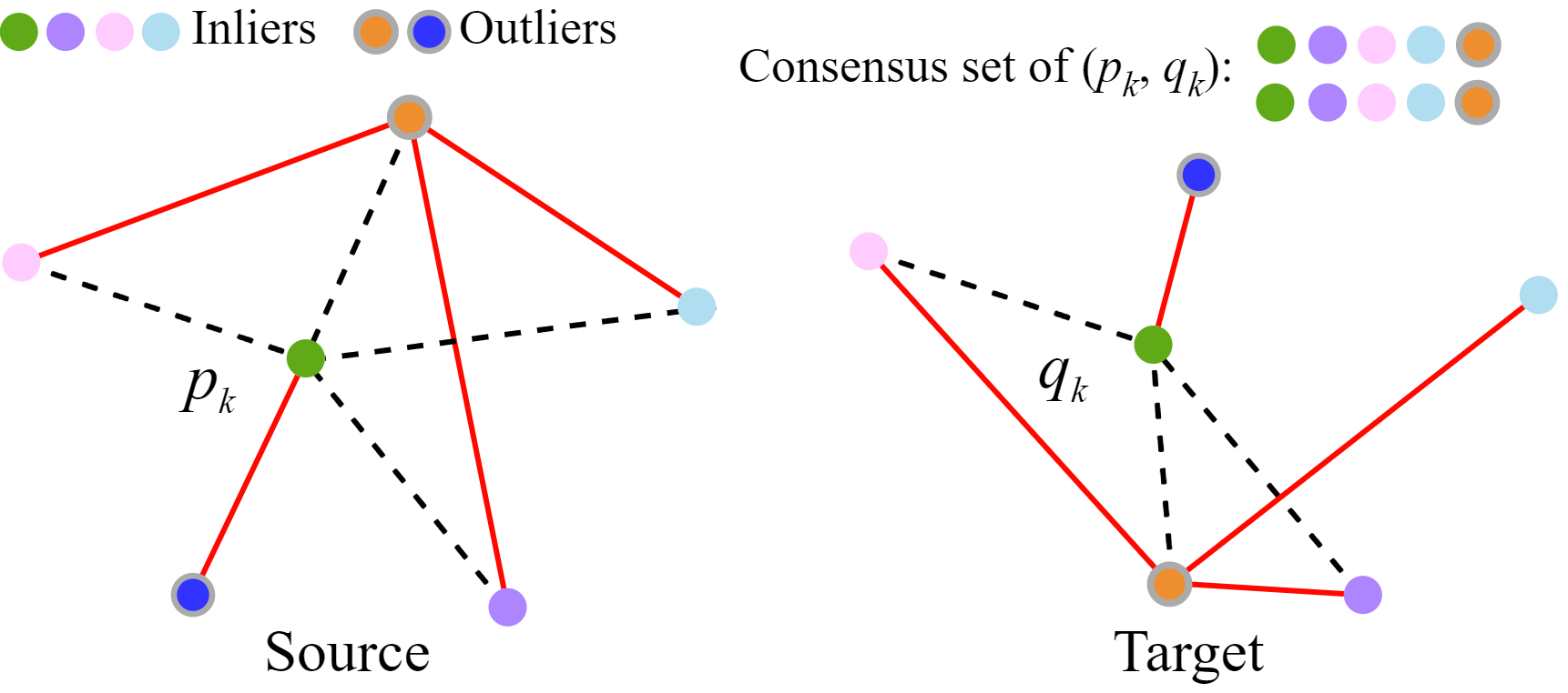
Consensus Verification. Upon identifying a larger consensus during the iteration, we update the minimal iteration requirement .
| (4) |
where superscript (1) indicates one-point sampling. denotes the current optimal consensus set. When the iteration number surpasses , the algorithm terminates and outputs .
III-D Two-point RANSAC
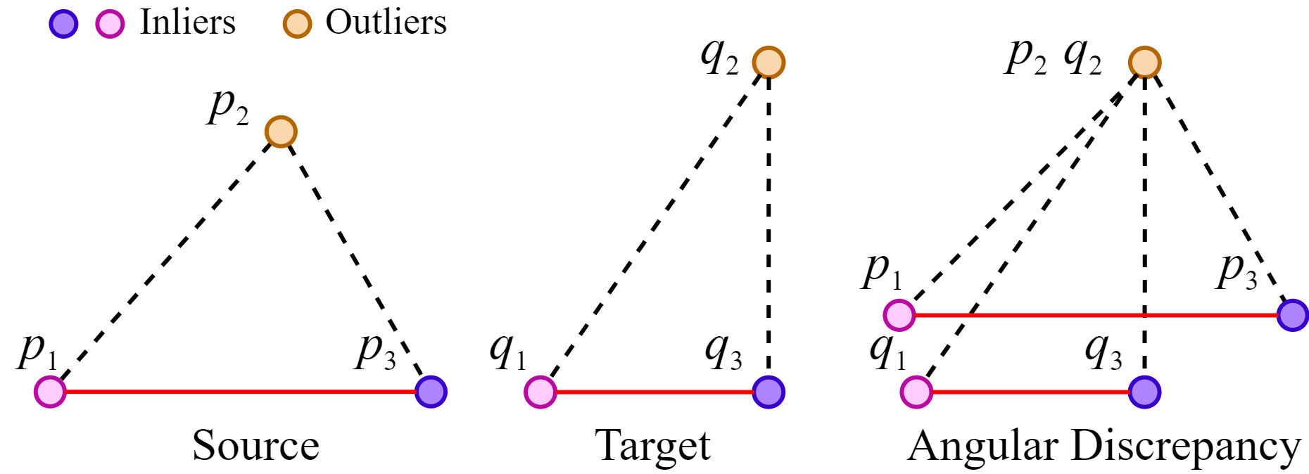
While the consensus set meets length requirements, outliers like the yellow correspondence still exist. Thus, we propose a two-point RANSAC to refine the consensus. As summarized in Algorithm 2, two-point RANSAC takes the result of one-point RANSAC as input and excludes outliers based on angle consistency. The main steps are as follows:
Two-point Subset Sampling. We begin by randomly selecting two different point correspondences, and from . Then, we compare them with others to collect a subset that simultaneously satisfies two length consistencies:
| (5) |
where is a correspondence subset of . is the length discrepancy in Eq. (3).
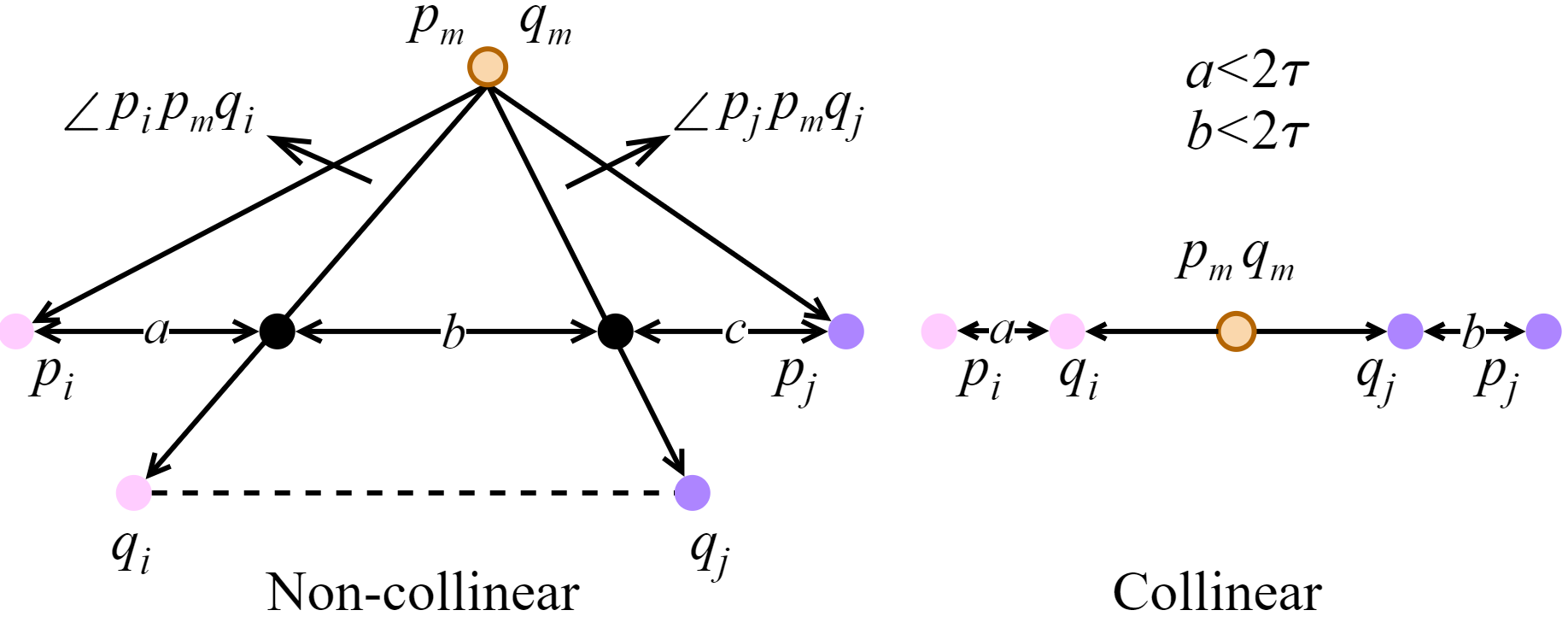
Consensus Generation As illustrated in Fig. 5, despite two edge correspondences maintaining length consistency, two triangles still exhibit distinct shapes due to angle discrepancy. Therefore, we propose angle consistency to encourage point correspondences to form roughly congruent triangles, yielding a more robust consensus set .
| (6) |
| (7) |
| (8) |
where means the current iteration number. denotes the angle disparity. Fig. 6 depicts the computation of and two cases of correspondence distribution.
Consensus Verification. This step is similar to that of the one-point RANSAC. Upon identifying a larger inlier set during the iteration, we immediately update the iteration’s termination condition .
| (9) |
This step is similar to that of the one-point RANSAC. Upon identifying a larger inlier set during the iteration, we immediately update the iteration’s termination condition .
III-E Three-point RANSAC
After one-point and two-point RANSAC, we obtain a correspondence subset satisfying length and angle constraints. Despite a notable increase in the inlier ratio, outliers may remain. Hence, we use three-point RANSAC to identify a consensus set based on the distances of transformed correspondences.
| (10) | ||||
where means the iteration number. represents a correspondence subset, and denotes a point correspondence. We employ singular value decomposition (SVD) to compute the rotation matrix and translation vector from three non-collinear correspondences.
III-F Scale-adaptive Cauchy IRLS
Input: Correspondences
Initialize: , , ,
Output: Transformation
Traditional Cauchy estimation exhibits considerable deviation from the ground truth in the first iteration if the outliers exceed 50. Correct inliers incur higher residuals and receive smaller weights. To address this, we introduce a scale-adaptive Cauchy IRLS[42] in Algorithm 3. We start by assigning equal weights () to all correspondences (). We then progressively lower the residual threshold based on a scale factor () and preserve inliers (). decreases continuously via the constant . Upon iteration termination, we output the optimal transformation (). Unlike FGR[4], scale-adaptive Cauchy IRLS uses a novel Cauchy objective function and automatically excludes outliers with control parameters during optimization. Additionally, it provides the applications of space intersection, robust feature matching, and point cloud registration.
IV Experiments
| Sequences | Type | (m) | Pairs (/) | (/) | (/) | |
| ETH | Arch | Outdoor | 16.48 | 8 | 6989 | 1.1% |
| Courtyard | Outdoor | 16.63 | 28 | 9910 | 6.1% | |
| Facade | Outdoor | 4.06 | 21 | 2250 | 12.2% | |
| Office | Indoor | 7.49 | 8 | 2964 | 5.6% | |
| Trees | Outdoor | 10.64 | 10 | 8242 | 1.2% | |
| KITTI | 01 | Highway | 16.97 | 200 | 3343 | 2.4% |
| 02 | Urban+Country | 16.97 | 200 | 3104 | 3.5% | |
| 03 | Country | 17.02 | 200 | 3175 | 4.6% | |
| 06 | Urban | 16.95 | 200 | 3655 | 3.6% | |
| 09 | Urban+Country | 16.96 | 200 | 3042 | 3.8% | |
IV-A Experimental Setup
Datasets. As summarized in Table I, we select ETH[43] and KITTI[44] for validation. The ETH dataset comprises 32 scans from five scenes (office, facade, courtyard, arch, and trees), acquired using Z + F Imager 5006i and Faro Focus 3D scanners. The KITTI dataset provides 11 Velodyne HDL-64E LiDAR sequences across diverse scenarios. We choose sequences 01 (highway), 02 (urban+country), 03 (country), 06 (urban), and 09 (urban+country). We randomly sample 200 pairs of point clouds per sequence.
Evaluation Metrics. We evaluate all methods via registration recall (), rotation error (), and translation error ():
| (11) | ||||
where is the matrix trace. and denote translation and rotation, respectively. Subscript denotes ground-truth values while represents estimated ones. is the count of successfully registered point cloud pairs while is the total number. Registration is successful if on the ETH dataset, and on the KITTI dataset.
Implementation Details. We select RANSAC10K[24], RANSAC50K[24], TEASER[19], SC2-PCR[1], MAC[2], and PCR-99[29] for comparisons. We implement our method in C++ on Ubuntu 20.04, running all experiments on an Intel Core i9-10850K CPU. For ETH, we downsample each point cloud with 0.1m voxels, then extract ISS[45] keypoints and FPFH[27] descriptors. We apply 0.3m voxels for KITTI, randomly sample 5,000 points, and extract FPFH[27] descriptors. Two points qualify as a correspondence if their descriptors rank in each other’s top three. We set as the point cloud’s resolution. The maximal distance for a valid correspondence is 0.3m in the ETH dataset and 0.6m for the KITTI dataset.
IV-B Results on ETH
| Methods | Arch | Courtyard | Facade | Office | Trees | |||||||||||||||
| time | time | time | time | |||||||||||||||||
| (%) | (°) | (m) | (ms) | (%) | (°) | (m) | (ms) | (%) | (°) | (m) | (ms) | (%) | (°) | (m) | (ms) | (%) | (°) | (m) | (ms) | |
| RANSAC10K | 89 | 0.47 | 0.12 | 3863 | 100 | 0.41 | 0.09 | 1802 | 90 | 1.35 | 0.16 | 2022 | 20 | 1.11 | 0.20 | 3470 | ||||
| RANSAC50K | 38 | 0.72 | 0.28 | 16263 | 100 | 0.21 | 0.10 | 18981 | 100 | 0.30 | 0.07 | 9047 | 90 | 1.23 | 0.22 | 10243 | 40 | 1.46 | 0.21 | 17752 |
| TEASER | 63 | 0.25 | 0.07 | 318 | 100 | 0.06 | 0.04 | 521 | 100 | 0.22 | 0.03 | 67 | 90 | 0.70 | 0.07 | 81 | 70 | 0.12 | 0.03 | 391 |
| SC2PCR | 88 | 0.18 | 0.06 | 6548 | 100 | 0.04 | 0.04 | 7383 | 100 | 0.08 | 0.02 | 693 | 100 | 0.45 | 0.04 | 1204 | 90 | 0.16 | 0.03 | 8699 |
| MAC | 88 | 0.09 | 0.05 | 316444 | 100 | 0.04 | 0.04 | 797857 | 100 | 0.13 | 0.02 | 14881 | 100 | 0.50 | 0.06 | 63080 | 100 | 0.25 | 0.07 | 331587 |
| PCR-99 | 50 | 0.18 | 0.04 | 7718 | 100 | 0.05 | 0.04 | 13881 | 95 | 0.22 | 0.04 | 774 | 90 | 0.85 | 0.08 | 1362 | 50 | 0.15 | 0.04 | 10309 |
| Ours | 88 | 0.14 | 0.04 | 35 | 100 | 0.02 | 0.04 | 96 | 100 | 0.11 | 0.03 | 35 | 100 | 0.64 | 0.06 | 27 | 100 | 0.19 | 0.03 | 58 |
| Methods | 01 | 02 | 03 | 06 | 09 | |||||||||||||||
| time | time | time | time | |||||||||||||||||
| (%) | (°) | (m) | (ms) | (%) | (°) | (m) | (ms) | (%) | (°) | (m) | (ms) | (%) | (°) | (m) | (ms) | (%) | (°) | (m) | (ms) | |
| RANSAC10K | 42 | 1.10 | 0.42 | 2206 | 69 | 1.16 | 0.42 | 2073 | 97 | 1.06 | 0.35 | 2098 | 88 | 0.99 | 0.38 | 2232 | 85 | 1.25 | 0.36 | 2063 |
| RANSAC50K | 44 | 0.74 | 0.30 | 11102 | 73 | 0.97 | 0.36 | 10268 | 100 | 0.78 | 0.28 | 10295 | 87 | 0.75 | 0.29 | 10854 | 88 | 1.06 | 0.32 | 9931 |
| TEASER | 52 | 0.65 | 0.26 | 166 | 74 | 1.00 | 0.34 | 117 | 99 | 0.86 | 0.25 | 115 | 97 | 0.65 | 0.22 | 134 | 89 | 1.05 | 0.28 | 106 |
| SC2PCR | 49 | 0.36 | 0.21 | 1801 | 75 | 0.66 | 0.31 | 1338 | 100 | 0.55 | 0.23 | 1387 | 92 | 0.40 | 0.19 | 1829 | 90 | 0.66 | 0.23 | 1279 |
| MAC | 54 | 0.40 | 0.26 | 35632 | 74 | 0.72 | 0.35 | 29158 | 100 | 0.56 | 0.27 | 75199 | 95 | 0.42 | 0.22 | 112980 | 91 | 0.69 | 0.28 | 26109 |
| PCR-99 | 55 | 1.37 | 0.45 | 12219 | 60 | 1.59 | 0.43 | 5506 | 77 | 1.36 | 0.39 | 4355 | 65 | 1.45 | 0.43 | 10266 | 71 | 1.56 | 0.40 | 3078 |
| Ours | 65 | 0.54 | 0.25 | 79 | 75 | 0.73 | 0.34 | 58 | 100 | 0.65 | 0.25 | 63 | 98 | 0.48 | 0.21 | 53 | 90 | 0.73 | 0.25 | 45 |
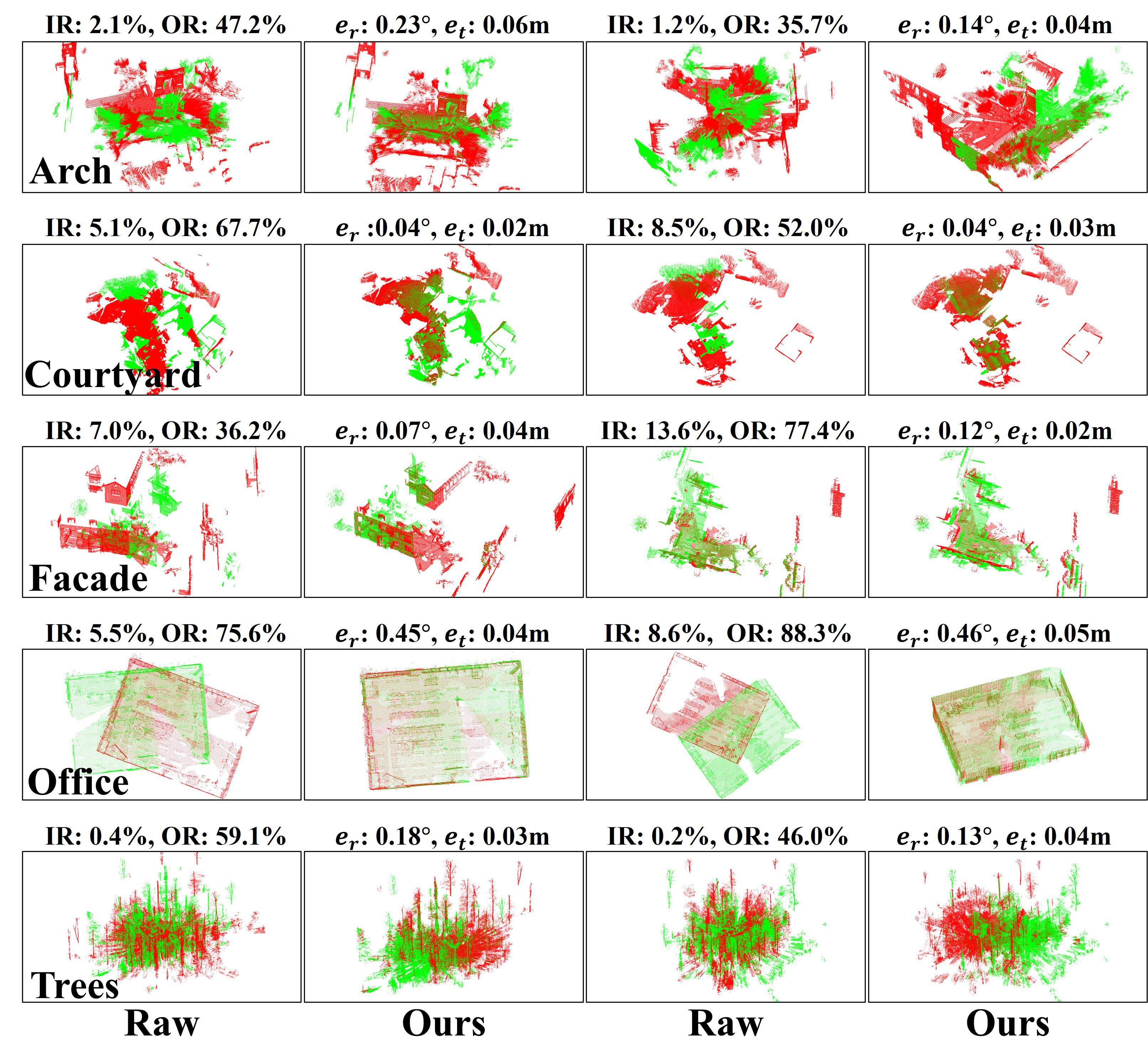
Recall and Accuracy. Fig. 7 depicts our registration results on the ETH dataset and Table II outlines the registration results. Courtyard, facade, and office have inlier ratios exceeding 5% while challenging arch and trees only have around 1%. Our method matches MAC in the recall, achieving top performance in all five scenarios (88% for arch and 100% for the others). It delivers the best translation accuracy in the arch (0.04m), courtyard (0.04m), and trees (0.03m), the second-best in the facade (0.03m) and office (0.06m). Our method also excels in rotational accuracy, leading in the courtyard (0.02°) and ranking second in the facade (0.11°). Our rotation error exceeds MAC, SC2PCR, and TEASER by 0.05°, 0.09°, and 0.07°in the arch, office, and trees, respectively. These results showcase that our method achieves comparable or superior registration accuracy and recall to mainstream methods.
Running Efficiency. Our method is generally two to three orders of magnitude faster than baseline methods. For example, on arch, it outperforms RANSAC50, SC2PCR, MAC, and PCR-99 by 465, 187, 9041, and 221 times, respectively. On the courtyard, it is 40, 198, 77, 8311, and 145 times faster than RANSAC10K, RANSAC50K, SC2PCR, MAC, and PCR-99, respectively. As MAC constructs a high-order graph and searches for the maximum clique, its time consumption significantly escalates with higher correspondence numbers and inlier ratios. In contrast, TCF shows minimal impact from correspondence quantity. It merely requires an additional 31ms and 69ms for trees and courtyard than the office, respectively, which underscores our high efficiency.
IV-C Results on KITTI
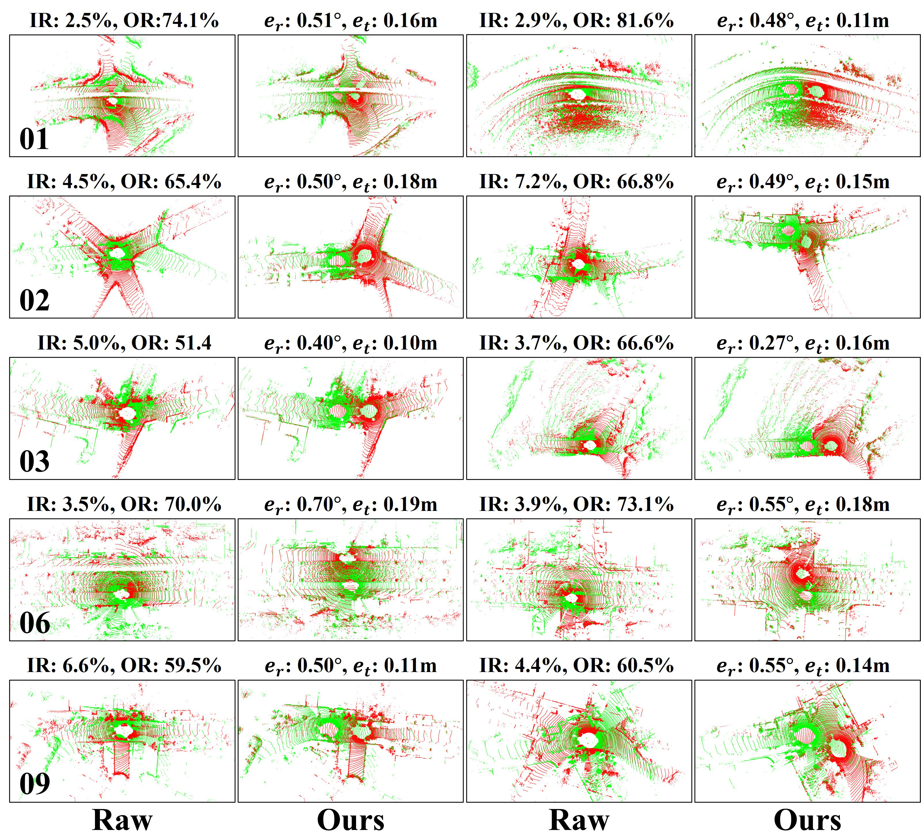
Recall and Accuracy. Table III summarizes the registration results on the KITTI dataset. Fig. 8 depicts our registration results. Due to the large offset (about 17m) between point clouds, all methods experience degradation. Sequence 01 is a high-speed scenario characterized by significant distortion and feature deterioration, resulting in a low inlier ratio of 2.4%. Despite this, our method achieves the highest recall (65%). It attains the second-highest translation accuracy across all five sequences: 0.25m (01), 0.34m (02), 0.25m (03), 0.21m (06), and 0.25m (09). Our rotation accuracy slightly lags behind SC2PCR and MAC but stays within a maximum deviation of 0.18°. These results underscore that our method excels in challenging environments like highways, exhibiting higher registration recall.
Running Efficiency. Our method still demonstrates superior efficiency. In sequence 01, it outperforms RANSAC10K, RANSAC50K, TEASER, SC2PCR, MAC, and PCR-99 by 28, 141, 2, 23, 451, and 155 times, respectively. Similarly, in sequence 06, our speeds surpass RANSAC10K, RANSAC50K, TEASER, SC2PCR, MAC, and PCR-99 by 42, 205, 3, 35, 465, 2132, and 194 times, respectively. In sequence 09, our method executes in 54ms, significantly outperforming RANSAC10K, RANSAC50K, TEASER, SC2PCR, MAC, and PCR-99, being 46, 221, 2, 28, 580, and 68 times faster, respectively. Our approach offers comparable or superior performance to baseline methods while significantly enhancing speed. The results demonstrate our effectiveness and efficiency with low-overlap data. Furthermore, these results reaffirm that our method elevates the RANSAC family to SOTA performance.
IV-D Boosting Performance with TCF
As illustrated in Table IV, we feed our consensus set into other methods to evaluate the registration performance. The total runtime in the table comprises ours and the baseline methods. Our approach reduces trees’ correspondences from 8,842 to 60, boosting the inlier ratio from 1.2% to 98%. All pipelines achieve 100% recall and stable registration, with deviations limited to 0.27° and 0.05m. TEASER and PCR-99 enhance the recall by 30% and 50%, respectively. TEASER, SC2PCR, MAC, and PCR-99 are 332ms, 9s, 330s, and 10s faster than their original methods, respectively. The correspondences in sequence 01 drop from 3343 to 121 while the inlier ratio jumps from 2.4% to 48%. TEASER, SC2PCR and MAC demonstrate 12%, 15%, and 10% recall improvement, respectively. TEASER, SC2PCR, MAC, and PCR-99 become faster by approximately 70ms, 2s, 30s, and 12s, respectively. The results prove that cascading our method with other methods effectively boosts registration performance and facilitates a qualitative leap in speed.
| Methods | Trees | 01 | ||||||
| time | time | |||||||
| (%) | (°) | (cm) | (ms) | (%) | (°) | (cm) | (ms) | |
| Ours+ TEASER | 100 | 0.24 | 0.05 | 59 | 64 | 0.54 | 0.25 | 96 |
| 30 | 0.11 | 0.01 | 332 | 12 | 0.07 | 0.09 | 70 | |
| \cdashline 1-9 Ours+ SC2PCR | 100 | 0.18 | 0.02 | 63 | 64 | 0.50 | 0.24 | 87 |
| 10 | 0.02 | 0.01 | 8636 | 15 | 0.14 | 0.03 | 1714 | |
| \cdashline 1-9 Ours+ MAC | 100 | 0.22 | 0.04 | 1672 | 64 | 0.51 | 0.24 | 5203 |
| 0.03 | 0.03 | 329915 | 10 | 0.11 | 0.02 | 30,429 | ||
| \cdashline 1-9 Ours+ PCR-99 | 100 | 0.27 | 0.04 | 59 | 63 | 0.94 | 0.33 | 121 |
| 50 | 0.03 | 0.02 | 10250 | 8 | 0.43 | 0.12 | 12098 | |
IV-E Ablation Study
Outlier Removal. Table V examines the contributions of our three RANSAC modules in outlier removal. IR is the inlier ratio while IN means the inlier number. In the arch, the slowest three-point RANSAC (3R) requires 3234ms and achieves an inlier ratio of 27%. The fastest one-point RANSAC (1R) completes in 20ms, delivering an inlier rate of 21%. Compared to 3R, 1R+2R+3R increases the inlier ratio by 58% and reduces runtime by 3202ms. In sequence 01, 1R remains the fastest, taking 29ms with 8% inliers. The slowest 3R requires 3139ms and achieves 28% inliers. 1R+2R+3R attains the highest inlier ratio at 38%, reduces runtime by 3089ms compared to 3R, and improves the inlier ratio by 30% relative to 1R. The results illustrate that our method decreases iterations for 3R and preserves a high inlier ratio.
PCR Performance. Table VI examines the contributions of 3R and IRLS to final registration performance. In Arch, 3R+IRLS reduces rotation errors by 0.06° and translation errors by 0.02m compared to using only 3R. It shows improvements of 0.04° and 0.01m upon IRLS. It takes only 1-2ms longer than 3R and IRLS. In sequence 06, 3R+IRLS enhances recall by 1% over other pipelines. Compared to 3R, it reduces angle error by 0.35° and translation error by 0.07m. Compared to IRLS, it reduces errors by 0.12° and 0.02m. It takes just an extra 4ms than the fastest 3R. These results indicate: (1) with most outliers removed by 1R+2R, the subsequent registration converges quickly, and (2) our overall pipeline (1R+2R+3R+IRLS) balances accuracy and efficiency.
| RANSAC Module | Arch | 01 | ||||
| IR (%) | IN (/) | Time (ms) | IR (%) | IN (/) | Time (ms) | |
| 1R | 21 | 76 | 20 | 8 | 57 | 29 |
| 2R | 26 | 48 | 672 | 12 | 27 | 115 |
| 3R | 27 | 16 | 3234 | 28 | 24 | 3139 |
| 1R+2R | 30 | 35 | 22 | 19 | 21 | 34 |
| 1R+3R | 63 | 57 | 25 | 35 | 47 | 43 |
| 2R+3R | 62 | 35 | 680 | 36 | 25 | 118 |
| 1R+2R+3R | 85 | 20 | 32 | 38 | 16 | 50 |
| 3R | IRLS | Arch | 06 | |||||||
| (%) | (°) | (m) | time (ms) | (%) | (°) | (m) | time (ms) | |||
| 1R+2R | ✓ | 88 | 0.19 | 0.06 | 30 | 74 | 0.86 | 0.30 | 39 | |
| 1R+2R | ✓ | 88 | 0.17 | 0.05 | 31 | 74 | 0.63 | 0.25 | 40 | |
| 1R+2R | ✓ | ✓ | 88 | 0.13 | 0.04 | 32 | 75 | 0.51 | 0.23 | 43 |
V Conclusion
We propose a two-stage consensus filtering method for correspondence-based registration. Our approach restores the RANSAC family to state-of-the-art (SOTA) performance. By combining length consistency with angle consistency, we effectively eliminate the majority of outliers, thus reducing the requisite iterations by three-point RANSAC. We combine three RASNAC modules and iterative weighted least squares into a complete registration pipeline that accelerates registration without compromising accuracy. Experimental results demonstrate a three-orders-of-magnitude speed enhancement while maintaining high registration quality. Moreover, integrating our method with existing approaches can notably improve efficiency and recall.
References
- [1] Z. Chen, K. Sun, F. Yang, and W. Tao, “Sc2-pcr: A second order spatial compatibility for efficient and robust point cloud registration,” in 2022 IEEE/CVF Conference on Computer Vision and Pattern Recognition (CVPR), 2022, pp. 13 211–13 221.
- [2] X. Zhang, J. Yang, S. Zhang, and Y. Zhang, “3d registration with maximal cliques,” in 2023 IEEE/CVF Conference on Computer Vision and Pattern Recognition (CVPR), 2023, pp. 17 745–17 754.
- [3] A. Zeng, S. Song, M. Nießner, M. Fisher, J. Xiao, and T. Funkhouser, “3dmatch: Learning local geometric descriptors from rgb-d reconstructions,” in 2017 IEEE Conference on Computer Vision and Pattern Recognition (CVPR), 2017, pp. 199–208.
- [4] Q.-Y. Zhou, J. Park, and V. Koltun, “Fast global registration,” in Computer Vision–ECCV 2016: 14th European Conference, Amsterdam, The Netherlands, October 11-14, 2016, Proceedings, Part II 14. Springer, 2016, pp. 766–782.
- [5] Y. Wang, P. Zhou, G. Geng, L. An, and Y. Liu, “Ccag: End-to-end point cloud registration,” IEEE Robotics and Automation Letters, vol. 9, no. 1, pp. 435–442, 2024.
- [6] P. Shi, Q. Ye, and L. Zeng, “A novel indoor structure extraction based on dense point cloud,” ISPRS International Journal of Geo-Information, vol. 9, no. 11, p. 660, 2020.
- [7] P. Shi, J. Li, and Y. Zhang, “Lidar localization at 100 fps: A map-aided and template descriptor-based global method,” International Journal of Applied Earth Observation and Geoinformation, vol. 120, p. 103336, 2023.
- [8] Q. Ye, P. Shi, K. Xu, P. Gui, and S. Zhang, “A novel loop closure detection approach using simplified structure for low-cost lidar,” Sensors, vol. 20, no. 8, p. 2299, 2020.
- [9] P. Shi, J. Li, and Y. Zhang, “A fast lidar place recognition and localization method by fusing local and global search,” ISPRS Journal of Photogrammetry and Remote Sensing, vol. 202, pp. 637–651, 2023.
- [10] P. Shi, Y. Xiao, W. Chen, J. Li, and Y. Zhang, “A new horizon: Employing map clustering similarity for lidar-based place recognition,” IEEE Transactions on Intelligent Vehicles, 2024.
- [11] Z. J. Yew and G. H. Lee, “Regtr: End-to-end point cloud correspondences with transformers,” in Proceedings of the IEEE/CVF conference on computer vision and pattern recognition, 2022, pp. 6677–6686.
- [12] G. Elbaz, T. Avraham, and A. Fischer, “3d point cloud registration for localization using a deep neural network auto-encoder,” in Proceedings of the IEEE conference on computer vision and pattern recognition, 2017, pp. 4631–4640.
- [13] Y. Zhang, P. Shi, and J. Li, “3d lidar slam: A survey,” The Photogrammetric Record, 2024.
- [14] P. Shi, Y. Zhang, and J. Li, “Lidar-based place recognition for autonomous driving: A survey,” arXiv preprint arXiv:2306.10561, 2023.
- [15] P. Besl and N. D. McKay, “A method for registration of 3-d shapes,” IEEE Transactions on Pattern Analysis and Machine Intelligence, vol. 14, no. 2, pp. 239–256, 1992.
- [16] F. A. Maken, F. Ramos, and L. Ott, “Stein icp for uncertainty estimation in point cloud matching,” IEEE robotics and automation letters, vol. 7, no. 2, pp. 1063–1070, 2021.
- [17] P. Shi, Q. Ye, Z. Shaoming, and D. Haifeng, “Localization initialization for multi-beam lidar considering indoor scene feature,” Acta Geodaetica et Cartographica Sinica, vol. 50, pp. 1594–1604, 2021.
- [18] P. SHI, J. LI, X. LIU, and Y. ZHANG, “Indoor cylinders guided lidar global localization and loop closure detection,” Geomatics and Information Science of Wuhan University, vol. 49, no. 7, pp. 1088–1099, 2024.
- [19] H. Yang, J. Shi, and L. Carlone, “Teaser: Fast and certifiable point cloud registration,” IEEE Transactions on Robotics, vol. 37, no. 2, pp. 314–333, 2021.
- [20] S. Quan and J. Yang, “Compatibility-guided sampling consensus for 3-d point cloud registration,” IEEE Transactions on Geoscience and Remote Sensing, vol. 58, no. 10, pp. 7380–7392, 2020.
- [21] S. Huang, Z. Gojcic, M. Usvyatsov, A. Wieser, and K. Schindler, “Predator: Registration of 3d point clouds with low overlap,” in 2021 IEEE/CVF Conference on Computer Vision and Pattern Recognition (CVPR), 2021, pp. 4265–4274.
- [22] Y. Wang and J. M. Solomon, “Deep closest point: Learning representations for point cloud registration,” in Proceedings of the IEEE/CVF international conference on computer vision, 2019, pp. 3523–3532.
- [23] J. Li, P. Shi, Q. Hu, and Y. Zhang, “Qgore: Quadratic-time guaranteed outlier removal for point cloud registration,” IEEE Transactions on Pattern Analysis and Machine Intelligence, vol. 45, no. 9, pp. 11 136–11 151, 2023.
- [24] M. A. Fischler and R. C. Bolles, “Random sample consensus: a paradigm for model fitting with applications to image analysis and automated cartography,” Communications of the ACM, vol. 24, no. 6, pp. 381–395, 1981.
- [25] O. Chum, J. Matas, and J. Kittler, “Locally optimized ransac,” in Pattern Recognition: 25th DAGM Symposium, Magdeburg, Germany, September 10-12, 2003. Proceedings 25. Springer, 2003, pp. 236–243.
- [26] J. Matas and O. Chum, “Randomized ransac with sequential probability ratio test,” in Tenth IEEE International Conference on Computer Vision (ICCV’05) Volume 1, vol. 2. IEEE, 2005, pp. 1727–1732.
- [27] R. B. Rusu, N. Blodow, and M. Beetz, “Fast point feature histograms (fpfh) for 3d registration,” in 2009 IEEE international conference on robotics and automation. IEEE, 2009, pp. 3212–3217.
- [28] D. Barath and J. Matas, “Graph-cut ransac,” in 2018 IEEE/CVF Conference on Computer Vision and Pattern Recognition, 2018, pp. 6733–6741.
- [29] S. H. Lee, J. Civera, and P. Vandewalle, “Pcr-99: A practical method for point cloud registration with 99% outliers,” arXiv preprint arXiv:2402.16598, 2024.
- [30] P. C. Lusk, K. Fathian, and J. P. How, “Clipper: A graph-theoretic framework for robust data association,” in 2021 IEEE International Conference on Robotics and Automation (ICRA). IEEE, 2021, pp. 13 828–13 834.
- [31] J. Shi, H. Yang, and L. Carlone, “Robin: a graph-theoretic approach to reject outliers in robust estimation using invariants,” in 2021 IEEE International Conference on Robotics and Automation (ICRA). IEEE, 2021, pp. 13 820–13 827.
- [32] Y. Chen and G. Medioni, “Object modelling by registration of multiple range images,” Image and vision computing, vol. 10, no. 3, pp. 145–155, 1992.
- [33] A. Segal, D. Haehnel, and S. Thrun, “Generalized-icp.” in Robotics: science and systems, vol. 2, no. 4. Seattle, WA, 2009, p. 435.
- [34] J. Yang, H. Li, D. Campbell, and Y. Jia, “Go-icp: A globally optimal solution to 3d icp point-set registration,” IEEE Transactions on Pattern Analysis and Machine Intelligence, vol. 38, no. 11, pp. 2241–2254, 2016.
- [35] H. Yang, P. Antonante, V. Tzoumas, and L. Carlone, “Graduated non-convexity for robust spatial perception: From non-minimal solvers to global outlier rejection,” IEEE Robotics and Automation Letters, vol. 5, no. 2, pp. 1127–1134, 2020.
- [36] Y. Wang, Y. Sun, Z. Liu, S. E. Sarma, M. M. Bronstein, and J. M. Solomon, “Dynamic graph cnn for learning on point clouds,” ACM Transactions on Graphics (tog), vol. 38, no. 5, pp. 1–12, 2019.
- [37] O. Vinyals, M. Fortunato, and N. Jaitly, “Pointer networks,” Advances in neural information processing systems, vol. 28, 2015.
- [38] C. Choy, J. Park, and V. Koltun, “Fully convolutional geometric features,” in Proceedings of the IEEE/CVF international conference on computer vision, 2019, pp. 8958–8966.
- [39] H. Deng, T. Birdal, and S. Ilic, “Ppfnet: Global context aware local features for robust 3d point matching,” in Proceedings of the IEEE conference on computer vision and pattern recognition, 2018, pp. 195–205.
- [40] ——, “Ppf-foldnet: Unsupervised learning of rotation invariant 3d local descriptors,” in Proceedings of the European conference on computer vision (ECCV), 2018, pp. 602–618.
- [41] M. Marcon, R. Spezialetti, S. Salti, L. Silva, and L. Di Stefano, “Unsupervised learning of local equivariant descriptors for point clouds,” IEEE Transactions on Pattern Analysis and Machine Intelligence, vol. 44, no. 12, pp. 9687–9702, 2021.
- [42] L. Jiayuan, Z. Yongjun, A. Mingyao, and H. Qingwu, “Scale-adaptive cauchy robust estimation based on progressive optimization and its applications,” Acta Geodaetica et Cartographica Sinica, vol. 52, no. 1, pp. 61–70, 2023.
- [43] P. W. Theiler, J. D. Wegner, and K. Schindler, “Globally consistent registration of terrestrial laser scans via graph optimization,” ISPRS journal of photogrammetry and remote sensing, vol. 109, pp. 126–138, 2015.
- [44] A. Geiger, P. Lenz, and R. Urtasun, “Are we ready for autonomous driving? the kitti vision benchmark suite,” in 2012 IEEE Conference on Computer Vision and Pattern Recognition, 2012, pp. 3354–3361.
- [45] Y. Zhong, “Intrinsic shape signatures: A shape descriptor for 3d object recognition,” in 2009 IEEE 12th international conference on computer vision workshops, ICCV Workshops. IEEE, 2009, pp. 689–696.