Abstract

Privacy and regulatory constraints make data generation vital to advancing machine learning without relying on real-world datasets. A leading approach for tabular data generation is the Forest Flow (FF) method, which combines Flow Matching with XGBoost. Despite its good performance, FF is slow and makes errors when treating categorical variables as one-hot continuous features. It is also highly sensitive to small changes in the initial conditions of the ordinary differential equation (ODE). To overcome these limitations, we develop Heterogeneous Sequential Feature Forest Flow (HS3F). Our method generates data sequentially (feature-by-feature), reducing the dependency on noisy initial conditions through the additional information from previously generated features. Furthermore, it generates categorical variables using multinomial sampling (from an XGBoost classifier) instead of flow matching, improving generation speed. We also use a Runge-Kutta 4th order (Rg4) ODE solver for improved performance over the Euler solver used in FF. Our experiments with 25 datasets reveal that HS3F produces higher quality and more diverse synthetic data than FF, especially for categorical variables. It also generates data 21-27 times faster for datasets with $\geq 20\%$ categorical variables. HS3F further demonstrates enhanced robustness to affine transformation in flow ODE initial conditions compared to FF. This study not only validates the HS3F but also unveils promising new strategies to advance generative models.

1 Introduction

Tabular datasets, typically derived from surveys and experiments, are crucial in various fields. They support decision-making in finance, healthcare, climate science, economics, and social sciences by providing detailed and quantifiable insights necessary for informed analysis and strategy (Borisov et al., 2024). Generating tabular data is an important task as it improves the performance of machine learning models through data augmentation (Motamed et al., 2021), mitigates bias by addressing class imbalance (Juwara et al., 2024), and enhances data security (LEE et al., 2021), enabling institutions to share valuable information without compromising privacy.

However, as discussed in several papers, including (Kim et al., 2023; Kotelnikov et al., 2023; Jolicoeur-Martineau et al., 2024), the generation of tabular data presents unique challenges that are often more complex than those associated with other data types. Key issues related to tabular data include feature heterogeneity (the coexistence of continuous and categorical features), the typically small size of tabular datasets, the low signal-to-noise ratio, and missing values.

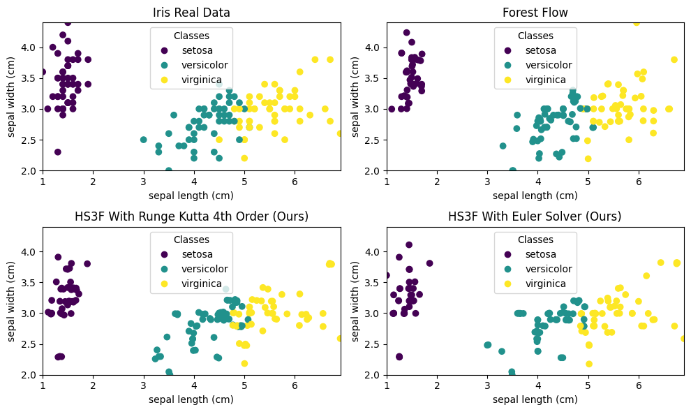
Figure 1: Iris Data: Three-Way Interaction Plot of Sepal Width vs. Length by Species, Comparing Real Data with Data Generated by ForestFlow, (Jolicoeur-Martineau et al., 2024), and by H3SF Using Euler and Runge Kutta 4th Order Solvers

Interestingly, significant advancements in AI have been made, especially in synthetic data generation, with the deployment of deep-generative models (DGMs), which are deep learning models capable of learning the underlying distribution and relationships within data, enabling the generation of new data mirroring these learned patterns. DGMs such as generative adversarial networks (GANs) (Goodfellow et al., 2014), variational autoencoders (VAEs)(Kingma and Welling, 2013), diffusion models (Sohl-Dickstein et al., 2015; Ho et al., 2020; Song et al., 2021) and conditional flow matching (CFM)(Lipman et al., 2023; Tong et al., 2023), were successfully used to handle tabular data generation.

One of the recent compelling methods for tabular data generation is conditional flow matching (CFM). CFM is an emerging generative modeling framework that is gaining prominence in AI-driven data generation, whose goal is to determine a flow that pushes a noisy sample distribution into the original data distribution. This process involves estimating vector fields conditioned on a data sample using a neural network, which, via an ODE, guides the trajectory of a flow that pushes the noise distribution to the target distribution.

Motivated by CFM, Jolicoeur-Martineau et al. (2024) deployed ForestFlow Matching (FF), a CFM-based tabular data generation method that uses eXtreme Gradient Boosting regressor models (XGBoost regressor (Chen and Guestrin, 2016)) for estimating conditional velocity vector fields instead of the typical neural networks. This non-deep-learning method produces highly realistic synthetic tabular data, even when the training dataset contains missing values. In an extensive study, the authors showed that FF outperforms many of the most effective and widely used deep-learning generative models while running with limited hardware (around 12-24 CPU cores, as found in a modern laptop).

Despite its efficiency, FF is slow and very sensitive to changes in the flow ODE initial condition (when the initial condition data distribution slightly differs from the Standard Gaussian). Additionally, FF does not effectively address feature heterogeneity. It handles discrete data by doing a one-hot encoding of the categories in order to relax the categorical distribution space into a continuous space. This solution is motivated by the fact that conditional flow matching is designed for typical continuous spaces. However, this solution leads to approximation errors for categorical data. As a result, FF tends to perform less effectively when there is a large number of categorical features in the data set.

Our method, heterogeneous sequential feature forest Flow (HS3F), extends ForestFlow (Jolicoeur-Martineau et al., 2024) through an explicit mechanism to handle heterogeneity. HS3F processes data sequentially (feature after feature). This allows us to generate continuous features using FF, but handle categorical features using a (Xgboost) classifier. Categorical features are generated by randomly sampling from the probabilities of the learned classifier, which massively improves speed and closeness to the real data distribution.

Our main contributions can be listed as follows:

• A novel and efficient Forest Flow framework denoted as heterogeneous sequential feature forest Flow (HS3F) that generates data one feature after the other, leveraging information from previously generated features.

• A natural, multinomial sampling for categorical features, based on the Xgboost classifier’s predicted class probability. This improvement avoids lifting the categorical space into a continuous, higher-dimensional space. Continuous features are generated via flow matching.

• An extensive data generation study (across 25 datasets) using various metrics. We demonstrate that HS3F produces higher quality and more diverse synthetic data than FF while significantly reducing computational time, especially when the data contains categorical features.

• An experimental demonstration that HS3F is more robust to distributional change in the flow ODE’s initial condition.

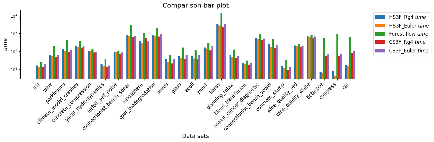
Figure 2: Data generation time comparison per models across generated datasets. We see that our proposed method HS3F is much faster than CS3F and Forest Flow, especially for datasets with many categorical features.

1.1 Related Work

Deep generative models have revolutionized tabular data generation by learning complex, nonlinear representations to generate highly realistic synthetic data. Among these, Generative Adversarial Networks (Goodfellow et al., 2014) (GANs) have been adapted for tabular data generation, leveraging architectures like Deep GANs, conditional GANs, and modified GANs to enhance data quality, privacy, and distribution preservation (Park et al., 2018; Esteban et al., 2017; Xu et al., 2019; Kim et al., 2021; Zhao et al., 2021; Yoon et al., 2019). Variational Autoencoders (Kingma and Welling, 2013) (VAEs) have also made significant contributions through extensions like TVAE, which employs a triple-loss objective to improve generation quality (Ishfaq et al., 2023). In recent advancements, diffusion-based models (Sohl-Dickstein et al., 2015; Song et al., 2021) and flow matching models (Lipman et al., 2023) have emerged as powerful tools for tabular data generation, often surpassing GANs and VAEs in performance. For example, the $TABDDM$ model utilizes Gaussian and multinomial diffusion for effective continuous and categorical data generation (Kotelnikov et al., 2023). The score-based diffusion model framework was also successfully adapted for tabular data generation through $STaSy$, which additionally employs self-paced learning to gain efficiency and better performance than $TABDDM$ (Song et al., 2021; Kim et al., 2023). Conditional Flow Matching (CFM) (Lipman et al., 2023) represents a newer approach that offers competitive performance and speed. In particular, Jolicoeur-Martineau et al. (2024) introduced the first flow-based model for tabular data generation using XGBoost regressors, known as Forest Flow (FF). Forest Flow (FF) has established itself as one of the best method in tabular data generation, showing exceptional performance in extensive studies across a wide range of datasets. Inspired by FF, we propose novel methods to advance this idea further.

The rest of this study is organized as follows. Section 2 presents the background of our study, including an introduction to flow matching and its variants. In Section 3, we discuss the methods used in this study, elaborating on the motivations behind their selection, and explaining each method. Section 4 presents the results obtained from our experiments. Finally, Section 5 concludes the study and suggests potential directions for future work that could make valuable contributions. Additional details and supplementary material are provided in the Appendix.

2 Background

This section introduces the flow matching framework, provides details on conditional flow matching and independent coupling flow matching, and discusses FF, the method that inspired our approach.

2.1 Conditional Flow Matching (CFM) Framework

2.1.1 Flow Matching

Let us assume that the data space is $\mathbb{R}^{n}$, with data points $x_{1}$ following the unknown distribution $q_{1}$, and the noisy data point $x_{0}$ following the distribution $p_{0}$. The motivation behind flow matching is to find a time-dependent probability path $p_{t},\,t\in[0,1]$ such that $p_{t=0}=p_{0}$ and $p_{t=1}=q_{1}$, assuming that this probability path is defined by a time-dependent map $\phi_{t}$ called flow which is induced by a time-dependent vector $v_{t}$ called velocity vector field, through the following flow ODE system (see Eq (1))

$$\dfrac{\partial\phi_{t}(x)}{dt}=v_{t}(\phi_{t}(x));\,\,\phi_{0}(x_{0})=x_{0}\sim p_{0},\,t\in[0,1].$$ (1)

$\phi_{t}$ determines the path $p_{t}$ via the relationship $p_{t}=[\phi_{t}]_{\#}p_{0}$ where $[]_{\#}$ is the push-forward relationship. The core concept of flow matching is the velocity vector field $v_{t}$, as it uniquely determines $\phi_{t}$ and therefore $p_{t}$ so that we can sample realistic data $\hat{x}_{1}\sim p_{1}$ given any $z\sim p_{0}$. Given a velocity vector $v_{t}$, the main objective of flow matching is then to regress a neural network $v^{\theta}_{t}:[0,1]\times\mathbb{R}^{d}\rightarrow\mathbb{R}^{d}$ against the velocity vector field $v_{t}$ by minimizing the loss function $\mathcal{L}_{FM}$ defined as follows:

$$\mathcal{L}_{FM}(\theta)=E_{t,p_{t}(x)}\|v_{t}(x_{t})-\hat{v}^{\theta}_{t}(x)\|^{2}.$$ (2)

After training, $\hat{v}^{\theta}_{t}$ is used to numerically solve the ODE (Eq.eq1) in order to determine the flow estimate $\hat{\phi}_{t}$ that pushes, through the push-forward relationship(Eq.(6)), $p_{0}$ to $q_{1}$.

Unfortunately, this flow-matching training objective is intractable because we do not have knowledge of suitable $v_{t}$ and $p_{t}$.

Conditional Flow Matching

To bypass this aforementioned tractability challenge, Lipman et al. (2023) suggested to instead minimize the conditional flow matching objective $\mathcal{L}_{CFM}$ (see 3) and demonstrated that $\mathcal{L}_{CFM}$ and $\mathcal{L}_{FM}$(Eq.(2)) have the same gradient:

$$\mathcal{L}_{CFM}(\theta)=E_{t,q(x_{1}),p_{t}(x|x_{1})}\|v^{\theta}_{t}(\phi_{t}(x|x_{1}))-v_{t}(x|x_{1})\|^{2},$$ (3)

where $q$ is some uniform distribution over the original data $x_{1}$, $p_{t}(x|x_{1})$ is a distribution equal to $p_{0}$ at time $t=0$ and centered in $x_{1}$ at time $t=1$ with mean $\mu_{t}$ and standard deviation $\sigma_{t}$, $v_{t}(x|x_{1})$ is the conditional velocity vector that induced $p_{t}(x|x_{1})$ via the linear conditional flow $x_{t}=\phi_{t}(x|x_{1})=\mu_{t}(x_{1})+x\sigma_{t}(x_{1})$.

Independent Coupling Flow Matching:

Tong et al. (2023) proposed the independent coupling flow matching (ICFM), a modified conditional flow matching method that provides better and faster flow directions. The ICFM framework assumes that $x_{0}$ and $x_{1}$ are sampled independently, $p_{t}(x|x_{0},x_{1})$ is a Gaussian distribution with expectation $\mu_{t}(x_{0},x_{1})=(1-t)x_{0}+tx_{1}$ and standard deviation $\sigma_{t}(x_{0},x_{1})=\sigma\in[0,1]$, and a corresponding linear flow $x_{t}=\mu_{t}(x_{0},x_{1})+x\sigma_{t}(x_{0},x_{1})$ which is induced by the conditional velocity vector $v_{t}(x|x_{0},x_{1})=x_{1}-x_{0}$. ICFM approximates the velocity vector by regressing a neural network $v^{\theta}_{t}$ against $x_{1}-x_{0}$ at each time $t\in[0,1]$, which lead to minimizing the following loss function:

$$\mathcal{L}_{ICFM}(\theta)=E_{t,p((x_{0},x_{1})),p_{t}(x|(x_{0},x_{1}))}\|v^{\theta}_{t}(x_{t})-(x_{1}-x_{0})\|^{2}$$ (4)

2.1.2 Forest Flow (FF)

Forest Flow is a ICFM-based method (with $\sigma=0)$ developed by Jolicoeur-Martineau et al. (2024) that makes use of a Xgboost regressor model (Chen and Guestrin, 2016) $v^{t}_{\theta}$ to minimize the loss function $\mathcal{L}_{ICFM}$ defined in (Eq.(4)). Minimizing an unbiased estimate of $\mathcal{L}_{ICFM}$ requires a random sampling from the original data $x_{1}$ (per batch sampling) through the empirical risk minimization (approximation of the expectation through average loss per dataset).

In the case of neural network, the mini-batch stochastic gradient descent (SGD) framework requires a training per batch which allows for the minimization of an unbiased estimate of $\mathcal{L}_{ICFM}$. However, the Xgboost training does not use the mini-batch training strategy, it rather uses the whole data for training. Therefore, computing an unbiased estimate for $\mathcal{L}_{ICFM}$ in this case becomes challenging. However, because the minimization of $\mathcal{L}_{ICFM}$ involves minimizing an expectation over all possible noise-data pairs ($x_{0},x_{1}$), Jolicoeur-Martineau et al. (2024) chose to sample several Gaussian noisy data $x^{i}_{0}$ per data sample ($x_{1}$), with $x^{i}_{0}$ and $x_{1}$ having the same size (e.g. [d,n]).

Consequently, in case the number of sampled noisy data $z$ is $n_{s}$, this could be defined as a collection $C=\{(x^{i}_{0},x_{1})\mid i=0,\dots,n_{s}\}$ which is also equivalent to duplicating the data $x_{1}$ $n_{s}$ times and by this, creating a duplicated data $X_{1}$ and sample a Gaussian noise $X_{0}$ with size $[n_{s}\times d,n]$. The conditional flow is now defined as $X_{t}=(1-t)X_{0}+tX_{1}$ at time $t$ and used to minimize $\mathcal{L}_{ICFM}$ and then approximate the flow from $X_{0}$ to $X_{1}$ which is further rescaled unto the initial data size $[d,n]$.

3 Method

This section begins by elaborating on the continuous Sequential Feature Forest Flow (CS3F) method, starting with its motivation and then explaining the method in detail. The second part of the section discusses the heterogeneous Sequential Feature Forest Flow (HS3FM) method.

3.1 Continuous Sequential Feature Forest Flow (CS3F)

Let us consider the initial original dataset $x_{1}=\{x^{1},\dots,x^{K}\}\in\mathbb{R}^{n\times K}$ which has $K$ feature vectors, $D_{K}=\{1,\dots,K\}$ the set of indices of the features of $x_{1}$ and a set of standard Gaussian vectors $x_{0}=\{x^{k}_{0},\dots,x^{K}_{0}\}\in\mathbb{R}^{n\times K}$. In FF, an Xgboost regressor $v^{t}_{\theta}$ is trained to direct the trajectory of the flow $\hat{\phi}_{t}$ which primarily start from $x_{0}$ ($\hat{\phi}_{t=0}(x)=x_{0}$).

Input: Data $x_{1}=\{x^{1},\dots,x^{K}\}\in\mathbb{R}^{n\times K}$ (M continuous features and K-M categorical features), noise levels $n_{s}=50$, $t\in T_{level}$ ($T_{level}$ contains $n_{s}$ evenly spaced time values between 0 and 1).

for $k\quad\text{in}\quad[1,\dots,K]$ do

       (Training process)

      for $t\quad\text{in}\quad T_{level}$ do

            

            Sample $x^{k}_{noise}\sim\mathcal{N}(0,I_{n})$ and compute conditional flow $x^{k}_{t}=(1-t)x^{k}_{noise}+tx^{k}$, and velocity vector $v^{k}_{t}=x^{k}-x^{k}_{noise}$.

            Let $X_{k-1}=(x^{k}_{t},x^{1},\dots,x^{k-1})$, $X_{0}=x^{1}_{t}$ and initialize Xgboost regressor $f^{\theta^{k}_{t}}$

            Solve $\underset{\theta^{k}_{t}}{argmin}L_{2}\left(v^{k}_{t},f^{\theta^{k}_{t}}(X_{k-1})\right).$

      Store the $n_{s}$ trained models $\hat{f}^{\theta^{k}_{t}},\,\text{for each}\,\,k$

for $k\quad\text{in}\quad[1,\dots,K]$ do

       (Feature Generation process)

      for t in $T_{level}$ do

             Sample $z^{k}_{t}\sim\mathcal{N}(0,I_{n})$ and concatenate noisy vector with previously generated features $\tilde{X}_{k-1}=(z^{k}_{t},\tilde{x}^{1}_{1},\dots,\tilde{x}^{k-1}_{1})$, $\tilde{X}_{0}=z^{1}_{t}$

            Use $\tilde{x}^{k}_{t_{0}}=z^{k}_{t}$ as initial condition for the Euler or Runge Kutta Discretization of: $\left(\dfrac{\partial\tilde{x}^{k}_{t}}{\partial t}=\hat{f}^{\theta^{k}_{t}}(\tilde{X}_{k-1})\right)$

      We obtain the generated feature $\tilde{x}^{k}_{1}$

The generated data $\tilde{X}=\{\tilde{x}^{1}_{1},\dots,\tilde{x}^{K}_{1}\}$ is returned return $\tilde{X}$

Algorithm 1 Continuous Sequential Feature ForestFlow Algorithm

However, when the initial condition of the ODE (See Eq.(1)) slightly deviates from $x_{0}$, $v^{t}_{\theta}$ does not provide useful directions to $\hat{\phi}_{t}$ which results in an accumulation of approximation errors while solving the flow ODE and therefore to an ill-approximation of the probability path. This leads to a significant increase in the Wasserstein distance value between the generated and real data distribution (see table (4)).

The Continuous Sequential Feature Forest Flow (CS3F), is a FF approach developed to enhance the robustness of FF to change in ODE flow initial condition $(\hat{\phi}_{t=0}(x)=x_{0})$ by developing a per-feature autoregressive data generation which allows for the mitigation of the dependency on $(\hat{\phi}_{t=0}(x)=x_{0})$. Furthermore, it also improves generation quality and the speed of FF.

Generating features autoregressively through the FF strategy leads to training a different Xgboost model per feature $v^{\theta^{k}_{t}}$ (where $\theta^{k}_{t}$ is the per feature model parameter) that takes as input the per feature conditional flow $x^{k}_{t}=(1-t)x^{k}_{0}+tx^{k}$ combined with the feature $x^{1},\dots,x^{k-1}$, to learn the per feature velocity vector $v^{k}_{t}(x|x_{0}^{k},x^{k})=x^{k}-x^{k}_{0}$ for $k\in D_{K}$.

For each index $k\in D_{K}$ and for all time $t\in[0,1]$, we obtained a trained model $\hat{v}^{\theta^{k}_{t}}$ that has learned $x^{k}-x^{k}_{0}$. Afterward, the flow for generating the $kth$ feature vector( $\tilde{x}^{k}_{1}$) is determined by solving the following flow ODE $\dfrac{\partial\tilde{x}^{k}_{t}}{\partial t}=\hat{v}^{\theta^{k}_{t}}(z^{k}_{t}|\tilde{x}^{1}_{1},\cdots,\tilde{x}^{k-1}_{1})$.

Where $\hat{v}^{\theta^{k}_{t}}$ takes as input a noisy vector $z^{k}_{t}\sim p^{k}_{0}$ given the previously generated features $\{\tilde{x}^{1}_{t},\cdots,\tilde{x}^{k-1}_{t},\,t=1\}$. Given this formulation, the only time that the vector field $\hat{v}^{\theta^{k}_{t}}$ provides the direction of its induced flow $\hat{\phi}^{k}_{t}$ only from a typical noise vector $z^{k}_{t}$ is when $k=1$ (first feature generation). Otherwise, $\hat{v}^{\theta^{k}_{t}}$ always directs $\hat{\phi}^{k}_{t}$ relying not only on $z^{k}_{t}$ but also on the filtered information provided by the previously generated features $\{\tilde{x}^{1}_{1},\cdots,\tilde{x}^{k-1}_{1}\}$.

This framework reduces the dependency on the ODE noisy initial conditions $v^{k}_{noise}$ and enhances model robustness to change in ODE noisy initial condition and provides faster results. Additionally, it can provide highly realistic continuous data. At the end of this autoregressive generation, we obtain the complete generated data $\hat{X}=\{\tilde{x}^{1}_{1},\dots,\tilde{x}^{K}_{1}\}$ following a distribution similar to the original data $x_{1}$.

3.2 Heterogeneous Sequential Feature Forest Flow (HS3F)

In this part, $CS3F$ is only for continuous feature generation.

Let us assume that the data set $x_{1}$ contains $N_{c}$ discrete features and let $I_{cat}$ and $I_{cont}$ be the disjoints respective set of indices of categorical and continuous features in $x_{1}$ ($D_{K}=I_{cat}\bigcup I_{cont}$). Let us denote by $v_{cat}=\{x^{k}\mid k\in I_{cat}\}\in x_{1}$, the set of all categorical features in $x_{1}$.

To generate discrete features $\tilde{x}^{k},\,k\in I_{cat}$ we first of all, respectively train different Xgboost classifiers $f^{\theta^{k}_{t}}$ to learn each discrete features $x^{k}\in V_{cat}$ using the previous features $X_{k-1}=\{x^{1},\dots,x^{k-1}\}$ as input.

After training, we use the previously generated features $\tilde{X}_{k-1}=\{\tilde{x}^{1},\dots,\tilde{x}^{k-1}\}$ as a test input to the trained classifier $\hat{f}^{\theta^{k}_{t}}$ and predict the class probabilities for each $x^{k}\in V_{cat}$, which are used as a proportion for a multinomial class sampling to generate each discrete feature.

Input: Data $x_{1}=\{x^{1},\dots,x^{K}\}\in\mathbb{R}^{n\times K}$ ($M$ continuous features, and $K-M$ categorical features), noise levels $n_{s}=50$, $t\in T_{level}$ ($T_{level}$ contains $n_{s}$ evenly spaced time values between 0 and 1).

for $k\quad\text{in}\quad[1,\dots,K]$ do

      

      if  $x^{k}$ is categorical then

             Get a Xgboost classifier model $f^{\theta^{k}}$

             Solve $\underset{\theta^{k}}{argmin}\,Loss\left(x^{k},f^{\theta^{k}}(x^{1},\dots,x^{k-1})\right)$

             Store the trained classifier models $\hat{f}^{\theta^{k}}$

      else

             Use CS3F training process for $f^{\theta^{k}_{t}}$ at the $n_{s}$ noise levels and store the $n_{s}$ trained regressor models $\hat{f}^{\theta^{k}_{t}}$ for each $k$,$t$

      

for $k\quad\text{in}\quad[1,\dots,K]$ do

       if $x^{k}$ is categorical then

             Get the predicted class probabilities from $\hat{f}^{\theta^{k}}(\tilde{x}^{1}_{1},\dots,\tilde{x}^{k-1}_{1}).$

             $\tilde{x}^{k}=Multinomial\left(\hat{f}^{\theta^{k}}(\tilde{x}^{1}_{1},\dots,\tilde{x}^{k-1}_{1})\right)$

      else

             Use the CS3F generation process to get $\tilde{x}^{k}=\tilde{x}^{k}_{1}$

      $\tilde{x}^{k}$ is the generated feature.

The generated data $\hat{X}=\{\tilde{x}^{1}_{1},\dots,\tilde{x}^{k}_{1}\}$ is returned

return $\hat{X}$

Algorithm 2 Heterogeneous Sequential FeatureForestFlow (HS3F) Algorithm

The Heterogeneous Sequential Feature Forest Flow (HS3F) uses CS3F for continuous features generation ($\tilde{x}^{k},k\in I_{cont}$) and the multinomial sampling-based Xgboost classifier afore-mentioned for categorical features ($\tilde{x}^{k},k\in I_{cat}$) sampling.

4 Experiments

All experiments used an 8-core CPU machine with 16 GB RAM with Python 3.11.4 (Van Rossum and Drake Jr, 1995). We use XGBoost as our prediction model, following Jolicoeur-Martineau et al. (2024).

The Xgboost classifier used $\eta=0.1$ as learning rate and 115 total trees. All other hyperparameters for the Xgboost regression model and classifier were left are their default values.

As is done in Jolicoeur-Martineau et al. (2024), we duplicated the rows of the dataset K = 100 times (note that this is unnecessary when the data set is entirely categorical) and we used $n_{s}=50$ noise levels.

We used conditional generation (generation conditioned to output labels for the classification dataset)(Jiang et al., 2014; Jolicoeur-Martineau et al., 2024) to improve the performance of our methods (not necessary as it provides similar performances with unconditional generation). We min-max scaled the continuous variable (only) of each data before passing them into our models, and then we unscaled the generated data.

We applied the same processing as FF for the generated continuous features (min-max scaling and clipping after generation). For the experiments, we compared FF to CS3F and HS3F with Euler or Runge-Kutta 4th order solvers (Akinsola, 2023). This leads to 4 variants of our methods that are denoted as $HS3FM$-based Euler solver (HS3F-Euler), $HS3FM$-based Runge-Kutta 4th order solver, (HS3F-Rg4), $CS3F$-based Euler solver (CS3F-Euler) and $CS3F$-based Runge-Kutta 4th order solver (CS3F-Rg4).

4.1 Assessment Metrics Description

Table 1: Metrics Information

Metric	Notation	Description	Purpose	Used Package
Rüschendorf (1985)	$W_{tr}$ and	Distance in distributions of	Distribution	POT
Wasserstein1 distance $\downarrow$	$W_{te}$	( $D^{fake}_{tr}$ vs $D^{real}_{tr}$) and ($D^{fake}_{tr}$ vs $D^{real}_{te}$ )	Preservation	(Flamary et al., 2021)
Goutte and Gaussier (2005)	$F1_{fake}$ and $F1_{comb}$	Classification performances of models trained	Usefulness for	Scikit-Learn
F1 Score $\uparrow$		on $D^{fake}_{tr}$ and $D^{Aug}_{tr}$ then tested on $D^{real}_{te}$	classification	(Pedregosa et al., 2011)
Ozer (1985) Coefficient of	$R2_{fake}$ and $R2_{comb}$	Fit quality metric for regression model trained	Usefulness for	Scikit-Learn
determination$\uparrow$		on $D^{fake}_{tr}$ and $D^{Aug}_{tr}$ then tested on $D^{real}_{te}$	regression	(Pedregosa et al., 2011)
Lohr (2012)Coverage $\uparrow$	coveragetr and	Measure of generation diversity ( $D^{fake}_{tr}$ vs $D^{real}_{tr}$)	Sample diversity	Pandas, Numpy, Scikit-Learn
	coveragete	and ($D^{fake}_{tr}$ vs $D^{real}_{te}$ )		(McKinney et al., 2010; Harris et al., 2020)
Running Time (in second)$\downarrow$	time	Determine the data generation process duration	Efficiency	(Python Software Foundation, 2024)

Table 2: Average post-generation metrics over 25 data sets (best in bold)

Models	$W_{tr}\downarrow$	$W_{te}\downarrow$	$R2_{fake}\uparrow$	$R2_{comb}\uparrow$	$F1_{fake}\uparrow$	$F1_{comb}\uparrow$	$coverage_{tr}\uparrow$	$coverage_{te}\uparrow$	time (sec)$\downarrow$
HS3F-Euler	1.283	1.949	0.580	0.668	0.738	0.775	0.787	0.846	278.425
CS3F-Euler	1.349	1.980	0.580	0.668	0.724	0.766	0.783	0.863	262.556
HS3F-Rg4	1.233	1.903	0.592	0.672	0.741	0.773	0.819	0.861	331.058
CS3F-Rg4	1.405	1.997	0.592	0.672	0.712	0.760	0.786	0.867	332.877
ForestFlow	1.356	1.898	0.606	0.659	0.723	0.766	0.839	0.894	1073.766

The original data set is divided into train ($D^{real}_{tr}$) and test data ($D^{real}_{te}$) and all model generation is based on $D^{real}_{tr}$. The generated data are denoted by $D^{fake}_{tr}$ and $D^{real}_{tr}$ augmented with $D^{fake}_{tr}$ will be denoted by $D^{Aug}_{tr}$.

We averaged the F1 score and the R-squared results of four classifiers/ regressors based on Adaboost, Random Forest, Xgboost and Logistic Regression trained on $D^{fake}_{tr}$ and $D^{Aug}_{tr}$ which resulted in two respective F1 scores ($F1_{fake}$ and $F1_{comb}$) and two respective R2 scores ($R2_{fake}$ and $R2_{comb}$).

We also determined the respective Wasserstein 1 distances (with L1 norm) between $D^{real}_{tr}$ to $D^{fake}_{tr}$ and from $D^{real}_{tr}$ to $D^{real}_{te}$ denoted by $W_{tr}$ and $W_{te}$. We also determined the respective coverage indicator (coverage_tr and coverage_te) of $D^{fake}_{tr}$ with respect to $D^{real}_{te}$ and $D^{fake}_{tr}$. Table (1) provides complementary information.

4.2 Comparison of Model Generation Using Default ODE Initialization in CFM (Standard gaussian)

We evaluated our methods on 25 real-world datasets from the UCI Machine Learning Repository (https://archive.ics.uci.edu/datasets) and scikit-Learn (Pedregosa et al., 2011) . Among these 25 data sets, 6 have continuous output, while the remaining ones (19) have categorical outputs. We compare the results of our four models to Forest Flow default approach (Jolicoeur-Martineau et al., 2024) using all the metrics described in table (1). To condensate the information, we average the result of each method over the 25 datasets and gather them in Table (2). To evaluate the performance of our methods on data having categorical features, we used the data sets among the 25 that have at least 20% of categorical features and we found five of them that are blood_transfusion(Yeh, 2008a), congress (UCI Machine Learning Repository, 1987), car (Bohanec, 1997), tictactoe (Aha, 1991), and glass (German and Spiehler, 1987). For comparison purposes, we recorded the performances of our methods along with the performance of ForestFlow on these data sets in table (3).

Table 3: Average post-generation metrics over five datasets (among the 25 used previously) blood_transfusion(Yeh, 2008a), congress (UCI Machine Learning Repository, 1987), car (Bohanec, 1997), tictactoe (UCI Machine Learning Repository, 1991), glass (German and Spiehler, 1987) having at least 20% of categorical variables (best in bold).

Models	$W_{tr}\downarrow$	$W_{te}\downarrow$	$F1_{fake}\uparrow$	$F1_{comb}\uparrow$	$coverage_{tr}\uparrow$	$coverage_{te}\uparrow$	time (sec) $\downarrow$
HS3F-Euler	0.596	1.321	0.763	0.787	0.788	0.671	17.612
CS3F-Euler	0.926	1.473	0.709	0.755	0.771	0.756	49.186
HS3F-Rg4	0.584	1.313	0.747	0.756	0.804	0.661	22.494
CS3F-Rg4	1.448	1.780	0.637	0.707	0.636	0.692	66.601
ForestFlow	1.064	1.461	0.703	0.747	0.700	0.735	468.352

Table 4: Sensitivity to ODE initial condition with $\Delta W=\mid W^{modified}-W^{default}\mid$ (best in bold).

Initial Conditions	$\Delta W_{tr}$ ($\downarrow$)			$\Delta W_{te}$ ($\downarrow$)
	HS3F-Rg4	CS3F-Rg4	ForestFlow	HS3F-Rg4	CS3F-Rg4	ForestFlow
$\mathcal{N}(0.1,(1.1)^{2}*I_{n})$	0.0085	0.0001	0.1462	0.02148	0.0001	0.1565
$\mathcal{N}(0.0,(0.9)^{2}*I_{n})$	0.0018	0.0006	0.03	0.0163	0.0007	0.049
$\mathcal{N}(0.0,(1.1)^{2}*I_{n})$	0.0028	0.0007	0.051	0.0154	0.0008	0.0497

From table (2), we can observe that HS3F-Rg4 outperformed the other methods across $W_{tr}$, $R2_{comb}$ and $F1_{fake}$, showcasing its ability to provide distribution-preserving generated samples through relatively more minor Wasserstein distances. It also demonstrates its usefulness for post-generation predictive experiments in regression and classification experiments through the R-squared and F1 scores. Across the other metrics, HS3F-Rg4 generally is the 2nd best method. HS3F-Euler closely follows the performances of HS3F-Rg4. Forestflow outperforms the other methods in terms of $W_{te}$, $coverage_{tr}$ and $coverage_{te}$ and $R2_{fake}$ indicating its ability to provide distribution preserving samples and can generalize better than the other methods. However, its performance in the remaining metrics is mostly ranked as the fourth-best method. We can also see that CS3F-Rg4 provided the worst overall performance in this experiment. The S3F-based Euler solver methods generate data faster than S3F-based Rg4 solver methods, which are significantly faster than Forest Flow (3.2 to 4.1 times faster).

Table (3) shows that for data sets with at least 20% of categorical features, HS3F-based models significantly outperform the other methods while delivering the fastest generation time. They generate data 20.82 to 26.59 times faster than ForestFlow, and their overall performance is followed by that of CS3F-based Euler solver and then Forestflow. Moreover, CS3F-Rg4 still achieves the poorest overall performance.

An intriguing insight from this experiment is the role of the CS3F-based models. While they may perform poorly when evaluated in isolation, they proved to be highly effective within the HS3F framework. Specifically, CS3F-Rg4 and CS3F-Euler contribute valuable, nuanced information that enhances the performance of Xgboost classifiers in this context. This fact is noticeable by comparing the performances of CS3F-Rg4 to HS3F-Rg4. This suggests that, despite its limitations, CS3F-Rg4 offers unique features that enrich the prediction for the Xgboost Classifiers predictions in HS3F, leading to improved discrete feature generation.

4.3 Wasserstein Distance Sensitivity to Affine Transformation In ODE Initialization

As discussed in the section (3.1), in the context of FF, when the velocity vector field is trained on a noisy data $x_{0}$ whose distribution differs from that of the flow ODE initial condition noisy data $(\phi_{t=0})$, the resulting flow is likely to have accumulated approximation errors that will result in an ill-approximation of the probability path and therefore lead to higher Wasserstein distance between the real and approximated data distribution (higher $W_{tr}$ and $W_{te}$).

To confirm our theory, we slightly modify the data distribution of the ODE flow initial condition using an affine transformation of the initial noisy data distribution $x_{0}$ (Standard Gaussian) leading to $\phi_{t=0}\sim\mathcal{N}(\mu=(0.1,\dots,0.1),\sigma^{2}=(1.1)^{2}*I_{n})$, $\phi_{t=0}\sim\mathcal{N}(\mu=(0.0,\dots,0.),\sigma^{2}=(0.9)^{2}*I_{n})$ and $\phi_{t=0}\sim\mathcal{N}(\mu=(0.0,\dots,0.),\sigma^{2}=(1.1)^{2}*I_{n})$. After that, we averaged the obtained Wasserstein train and test of Forest flow, CS3F-Rg4, and HS3F-Rg4 over the 25 data sets (aforementioned) and determined the Wasserstance distance difference between the modified and default initial conditions results in absolute values. The results are recorded in table (4) and compare them to the results obtained using the default initial condition (see table (2)).

The results of the experiment, as shown in table (4), confirm our theory showing that CS3F-Rg4 provides the most robust Wasserstein distance performance which is followed by HS3F-Rg4 and then comes ForestFlow which appears to be significantly impacted by the change.

5 Conclusion

In this work, we extended Forest Flow by addressing its existing limitations which are sensitivity to initial condition change and lack of efficient strategy to handle mixed type data.

Our experimental results confirmed that, compared to Forest Flow, HS3F yields methods that are more robust to affine change in the initial condition of the ODE flow and provides a more explicit and efficient way to handle mixed data types while improving overall data generation performance across several data sets and providing faster results.

This framework offers a new perspective on data generation using diffusion-based techniques, emphasizing the sequential generation of features and the utilization of information from previously generated features. HS3F represents a significant step forward in the field of data generation, offering new opportunities to improve the efficiency of generative models. Spurious features may negatively impact sequential generation. A helpful practice would be to determine which features are causally related and use only those in the sequential generation process.

6 More Details About the Conditional Flow Matching Concept

6.1 Flow Matching

Let us assume that the data space is $\mathbb{R}^{n}$, with data points $x_{1}$ following the unknown distribution $q_{1}$ over $\mathbb{R}^{n}$, and that the noisy data point is $x_{0}$ which follows the distribution $p_{0}$. The motivation behind flow matching is that there exists a time-dependent probability path $p_{t}$ such that $p_{t=0}=p_{0}$ and $p_{t=1}=q_{1}$, and the goal is to find this probability path. Flow matching assumes that given $x_{0}$, $p_{t}$ is induced by a time-dependent velocity vector field $v_{t}$, which, over time ($t\in[0,1]$), directs the trajectory of a time-dependent map $\phi_{t}$ that pushes, via the push-forward relationship (see Eq.(6)), the noisy distribution $p_{0}$ to $p_{t}$. $\phi_{t}$ in this case is the flow induced by $v_{t}$. Given $x_{t}\sim p_{t}$, the relationship between the velocity vector field $v_{t}(x_{t})$ and its induced flow $\phi_{t}$ can formally be defined by Eq.(5) which is an ordinary differential equation (ODE) which specifies that $v_{t}$ defines how quickly and in which direction $\phi_{t}$ evolves over time starting from the noisy data $x_{0}$:

$$\dfrac{\partial\phi_{t}(x)}{dt}=v_{t}(\phi_{t}(x));\quad\phi_{0}(x_{0})=x_{0}\sim p_{0},\,t\in[0,1].$$ (5)

The push-forward relationship defined by $\phi_{t}$ between $p_{0}$ and $p_{t}$ is represented as:

$$p_{t}(x_{t})=[\phi_{t}]_{\#}(p_{0})=p_{0}(\phi_{t}^{-1}(x_{t}))\cdot det\left|\dfrac{\partial\phi_{t}^{-1}(x_{t})}{\partial x}\right|.$$ (6)

When the Eq.(6) and Eq.(5) are satisfied for a given velocity vector field $v_{t}$ and its corresponding flow $\phi_{t}$ which pushes a distribution $p_{0}$ to the probability path $p_{t}$ at time $t\in[0,1]$, then $v_{t}$ is said to generate $p_{t}$. Formally, $v_{t}$ generates $p_{t}$ if it satisfies the continuity equation:

$$\frac{{\partial p_{t}(x)}}{{\partial t}}+\text{div}(p_{t}(x)v_{t}(x))=0.\quad$$ (7)

From [Eq.(5), Eq.(6) and Eq.(7)], we can conclude that the knowledge of a velocity vector field $v_{t}$ uniquely determines the probability path $p_{t}$. Therefore, instead of directly determining the right probability path $p_{t}$ so that $p_{1}\approx q_{1}$, which can be very challenging, the flow matching framework intends to approximate the velocity vector field $v_{t}$ that induces $p_{t}$. Given this information, the main objective of flow matching is to regress a neural network $v_{\theta}:[0,1]\times\mathbb{R}^{d}\rightarrow\mathbb{R}^{d}$ against the velocity vector field $v_{t}$ by minimizing the loss function $\mathcal{L}_{FM}$ (see Eq.(8)), in order to determine the flow $\hat{\phi}_{t}$ induced by the trained neural network, which defines a probability path $p_{t}$ from $p_{0}$ to $p_{1}$ which is similar to $q_{1}$, through the push-forward relationship(Eq.(6)). The training loss function of flow matching is defined as follows:

$$\mathcal{L}_{FM}(\theta)=E_{t,p_{t}(x)}\|v_{t}(x)-v_{\theta}(x)\|^{2}.$$ (8)

Thereafter, Eq.(5) has to be solved numerically (using the trained $v_{\theta}$) in order to determine the flow estimate $\hat{\phi}_{t}$ that pushes, through the push-forward relationship(Eq.(6)), $p_{0}$ to $p_{1}\approx q_{1}$.

Unfortunately, this flow-matching training objective is intractable because we do not have knowledge of suitable $v_{t}$ and $p_{t}$. Consequently, we can not have a suitable flow estimate $\hat{\phi}_{t}$ from this framework.

6.2 Conditional Flow Matching

To bypass this aforementioned tractability challenge, Lipman et al. (2023); Tong et al. (2023) suggested to construct $p_{t}$ as a mixture of simpler conditional probability path $p_{t}(x|z)$ which varies with some conditioning feature $z$ that depends on $x_{1}$, such that $p_{0}(x|z)=p_{0}$ and $p_{1}(x|z)=q_{1}(x)$. $p_{t}(x|z)$ is assumed to be generated by a conditional vector field $v_{t}(x|z)$ that induces a conditional flow $\phi_{t}(x|z)$ (from $x_{0}$ to $x_{t}$). Lipman et al. (2023); Tong et al. (2023) defined $p_{t}$ as the marginalization of $p_{t}(x|z)$ over $q(z)$, and determined a suitable velocity vector field $v_{t}$ based on $v_{t}(x|z)$ that generates $p_{t}$ ($v_{t}$ satisfies the continuity Eq.(7)), as follows:

$$p_{t}(x)=\mathbb{E}_{q(z)}[p_{t}(x|z)] \quad\text{and}\quad v_{t}(x)=\mathbb{E}_{q(z)}[v_{t}(x|z)\dfrac{p_{t}(x|z)}{p_{t}(x)}].$$ (9)

Unfortunately, the expression of $v_{t}(x)$ Eq.(9) cannot be used directly to solve Eq.(8) because the true $p_{t}(x)$ remains unknown. Therefore, computing an unbiased estimate of the flow matching loss function $\mathcal{L}_{FM}$ (Eq.(8)) is not possible. To overcome this challenge, Lipman et al. (2023) suggest to instead minimize the conditional flow matching objective $\mathcal{L}_{CFM}$ (see Eq.(10)) and demonstrated that $\mathcal{L}_{CFM}$ and $\mathcal{L}_{FM}$(Eq.(8)) have the same gradient:

$$\mathcal{L}_{CFM}(\theta)=E_{t,q(z),p_{t}(x|z)}\|v_{\theta}(\phi_{t}(x|z))-v_{t}(x|z)\|^{2}.$$ (10)

Therefore, regressing a neural network $v^{t}_{\theta}$ against $v_{t}(x|z)$ through $\mathcal{L}_{CFM}$ yields the same optimal solution as regressing $v^{t}_{\theta}$ against $v_{t}(x)$ through $\mathcal{L}_{FM}$.

For specificity purposes, it is worth mentioning that the conditional flow matching paradigm is entirely defined by the nature of the conditional probability path $p_{t}(x|z)$, the conditional velocity vector $v_{t}(x|z)$ and its induced condition flow $\phi_{t}(x|z)$ $\forall t\in[0,1]$ and also the conditioning feature $z$.

6.3 Gaussian Conditional Flow Matching

Gaussian conditional flow matching (GCFM) is a conditional flow matching concept introduced by Lipman et al. (2023), which assumes that the initial sample distribution is a standard Gaussian ($x_{0}\sim p_{0}=\mathcal{N}(x_{0}|0,I)$), makes Gaussian assumptions on the conditional probability path ($p_{t}(x|z)=\mathcal{N}(x|\mu_{t}(z),\sigma_{t}(z)^{2}Id_{n}))$), and assumes a linear conditional flow $(\phi_{t}(x_{0}|z)=\mu_{t}(z)+x_{0}\sigma_{t}(z))$ so that $\phi_{0}(x_{0}|z)=x_{0}$ and $\phi_{1}(x|z)=x_{1}$ and $z=x_{1}$. Lipman et al. (2023) demonstrated that for $\sigma_{t}(z)>0$ the unique conditional velocity flow $v_{t}(x|z)$ that induces $\phi_{t}(x|z)$ and generates $p_{t}(x|z)$ and has the form:

$$v_{t}(x|z)=\dfrac{1}{\sigma_{t}(z)}\dfrac{\partial\sigma_{t}(z)}{\partial t}(x-\mu_{t}(z))+\dfrac{\partial\mu_{t}(z)}{\partial t},$$ (11)

A variant of the GCFM is the Independent Coupling Flow Matching (ICFM) Tong et al. (2023) that provides better and faster flow directions. The ICFM framework assumes that $x_{0}$ and $x_{1}$ are sampled independently and $z=x_{0},x_{1})$, $p_{t}(x|x_{0},x_{1})$ is a Gaussian distribution with expectation $\mu_{t}(x_{0},x_{1})=(1-t)x_{0}+tx_{1}$ and standard deviation $\sigma_{t}(x_{0},x_{1})=\sigma\in[0,1]$, and a corresponding linear flow $x_{t}=\mu_{t}(x_{0},x_{1})+x\sigma_{t}(x_{0},x_{1})$ which is induced by the conditional velocity vector $v_{t}(x|x_{0},x_{1})=x_{1}-x_{0}$.

6.4 Conditional Flow Matching Algorithm and Motivation forCS3F

Input: $x_{1}$:real dataset, $q$: uniform distribution over $x_{1}$, $p_{0}$: noise distribution, initialized $v^{\theta}_{t}$

while not converged do

       $t\sim\mathcal{U}([0,1])$ ;

       $x_{1}\sim q(x_{1})$ ;

       $x_{0}\sim p_{0}(x_{0})$ [sample noise] ;

       $x_{t}=\phi_{t}(x_{0}\mid x_{1})$ [conditional flow] ;

       Gradient step with $\nabla_{\theta}\|v^{\theta}_{t}(x_{t})-\dot{x}_{t}\|^{2}$ ;

      

Output: $\hat{v}^{\theta}_{t}$

Algorithm 3 Conditional Flow Matching Training (Lipman et al., 2023)

Input: Trained model $\hat{v}_{t}^{\theta}$

$z_{0}\sim p_{0}(z_{0})$ [sample noise] ;

Numerically solve ODE $\dot{z}_{t}=\hat{v}^{\theta}_{t}(z_{t})$ ;

Output: $z_{t=1}$

Algorithm 4 Conditional Flow Matching Sampling

Consider that we have an initial dataset $x_{1}=\{x^{1},\dots,x^{K}\}\in\mathbb{R}^{d\times K}$ having $K$ features, $D_{K}=\{1,\dots,K\}$ is the set of indices of the features of $x_{1}$ and a standard Gaussian noisy data set $x_{0}=\{x^{k}_{0},\dots,x^{K}_{0}\}\in\mathbb{R}^{d\times K}$. Forest flow, as any other CFM-based method, determines the flow $\phi_{t}$ from a standard Gaussian noise $x_{0}$, to the real data $x_{1}$ by numerically solving an ODE (see Eq.(5)) but uses the prediction of the Xgboost regression model $v^{t}_{\theta}$ (instead of a neural network as for CFM-based methods) trained on the conditional flow $\phi_{t}(x|(x_{0},x_{1}))=(1-t)x_{0}+tx_{1},\,(t\in[0,1])$ to approximate the vector field $v_{t}$.

One condition for this framework to work is that the initial condition of the flow ODE (see Eq.(5)) should be equal or from the same distribution with $x_{0}$ ($z_{0}\sim p_{0}$). What would happen if the initial condition of the ODE flow was slightly modified from standard Gaussian to Gaussian with expectation $\mu=a\in\mathbb{R}$ and variance $\sigma^{2}=bI_{n}\in\mathbb{R}$ for instance? We experimentally proved that the performance in term of Wassertein distance will drop significantly. This concern is the main motivation for the deployment of CS3FM.

7 Sequential FeatureForestFlow Matching

7.1 Continuous Sequential FeatureForestFlow Matching

CS3F was deployed to make data generation more robust to changes in initial conditions. TheCS3Fis a ICFM-based method that handles data feature-wise generation sequentially. Let us assume that we have an initial dataset $x_{1}=\{x^{1},\dots,x^{K}\}\sim q_{1}$ that has $K$ features, $D_{K}=\{1,\dots,K\}$ the set of indices of the features of $x_{1}$ and the standard Gaussian noisy data set $x_{0}=\{x^{k}_{0},\dots,x^{K}_{0}\}\in\mathbb{R}^{d\times K}$ whose distribution is denoted as $p_{0}$. We assume that each of the features $x^{k}$ follow an unknown distribution $q^{k}_{1}$, and that each feature $x^{k}_{0}$ follows a standard Gaussian distribution denoted by $p^{k}_{0}$. Let us denote by $n_{s}$ the number of time steps $t$ that are used in the flow process and assume that $t\in T_{level}=\{t_{0},\dots,t_{n_{s}-2},t_{n_{s}-1}\}\in[0,1].$

Using a feature-wise ICFM framework $\forall k\in D_{K}$, we result in a per feature conditional variable $z^{k}=(x^{k}_{0},x^{k})$, Gaussian conditional probability paths, with their corresponding conditional velocity flows and calculated conditional velocity vectors, which are defined $\forall t\in T_{level}$ as follows.

$$p^{k}_{t}(x|z^{k}) =\mathcal{N}\left(x|z^{k},\mu^{k}_{t}=(1-t)x^{k}_{0}+tx^{k},\sigma^{k}_{t}=0\right),\,\,\,x^{k}_{t}=\phi^{k}_{t}(x|z^{k})=\mu^{k}_{t}\,\,and\,\,v^{k}_{t}(x|z^{k})=x^{k}-x^{k}_{0},$$

Continuous Sequential Feature Flow Matching (CS3F) Training :

For $x^{k}\in x_{1}$, we create $N=K*n_{s}$ input data by concatenating conditional flow vectors $x^{k}_{t}$ with previous features $\{x^{1},\dots,x^{k-1}\}$, $\forall t\in T_{levels}$ and use them to, respectively, train $N$ Xgboost regressor models: $f^{\theta^{k}_{t}}(x^{k}_{t},x^{1},\dots,x^{k-1})$ $\forall k\in D_{K},\,\,\forall t\in T_{levels}$, to learn the conditional vectors field $v^{k}_{t}(x|z^{k})=x^{k}-x^{k}_{0}$. For $x^{k}\in x_{1}$, the conditional feature flow matching training objective is :

$$\underset{\theta^{k}_{t}}{argmin}\mathbb{E}_{t,q(z^{k}),p^{k}_{t}(x|z^{k})}\left\|f^{\theta^{k}_{t}}[x^{k}_{t}|x^{1},\dots,x^{k-1}]-(x^{k}-x^{k}_{0})\right\|^{2},\,\,k\in D_{K}\,\textbf{and}\,\,\forall t\in T_{level}$$ (12)

It is worth noting that when k=1, the Xgboost model takes only $x^{1}_{t}$ as its input.

Model Generation:

After training, $\forall k\in D_{K}$, we obtain $N$ Xgboost models $(\hat{f}^{\theta^{k}_{t}})$ that learned $N$ velocity vectors $v^{k}_{t}(x|z^{k})$.

We first start by determining the flow that pushes the $p^{k}_{0}$ standard Gaussian distribution to a distribution $p^{k}_{1}$ which is similar to $q^{k}_{1}$, via the following ODE:

$$\dfrac{\partial\tilde{x}^{1}_{t}}{\partial t}=\hat{f}^{\theta^{1}_{t}}(z^{1}_{t}),\,\,z^{1}_{t}\sim\mathcal{N}(0,I_{n}),\,\,\tilde{x}^{1}_{t=0}=z^{1}_{t},\,\,\forall t\in T_{level},$$ (13)

Afterward, $\forall k\in\{2,\dots,K\}$, using as input the noisy vector $z^{k}_{t}\sim\mathcal{N}(0,I_{n})$ concatenated with the previous generated features $(\tilde{x}^{1}_{1},\cdots,\tilde{x}^{k-1}_{1})$, we numerically solve the following ODE:

$$\dfrac{\partial\tilde{x}^{k}_{t}}{\partial t} =\hat{f}^{\theta^{k}_{t}}(z^{k}_{t},\tilde{x}^{1}_{1},\cdots,\tilde{x}^{k-1}_{1}),\,\,\,\tilde{x}^{k}_{t=0}=z^{k}_{t},\,\,\forall t\in T_{level}.$$ (14)

The resulting $\tilde{v}^{k}$, is a generated sample whose distribution is similar to $x^{k},\,\,\forall k\in\{2,\dots,K\}$. At the end of this process, we obtain a generated data set $\tilde{X}_{1}=\{\tilde{x}^{1}_{1},\dots,\tilde{x}^{K}_{1}\}\sim p_{1}\approx q_{1}$.

7.2 Heterogeneous Sequential Feature Forest Flow Matching

Assuming that the data set $x_{1}$ contains $N_{c}$ categorical features and let $I_{cat}$ and $I_{cont}$ be the respective set of indices of categorical and continuous features in $x_{1}$ ($D_{K}=I_{cat}\bigcup I_{cont}$). Let us denote by $v_{cat}=\{x^{k}\mid k\in I_{cat}\}\in x_{1}$, the set of all categorical features in $x_{1}$. We train a different Xgboost classifier on each input data $X_{k-1}=\{x^{1},\dots,x^{k-1}\}$, to learn each categorical feature $x^{k}\in v_{cat}$. The training objective function can be expressed as

$$\underset{\theta^{k}}{argmin}\,ClassificationLoss\left(f^{\theta^{k}}(X_{k-1}),x^{{k}}\right),\,\,x^{k}\in v_{cat}$$ (15)

We obtained afterwards, $N_{c}$ different trained Xgboost classifiers $\hat{f}^{\theta^{k}}$ that respectively learned the $N_{c}$ categorical features $x^{k}\in v_{cat}$. For continuous features, we use the CS3F training for $(K-N_{c})\times n_{s}$ models.

Continuous Feature Generation Each continuous feature is generated using the CS3F data generation method.

Discrete Feature Generation For each $x^{k}\in V_{cat}$, after training, we use the previously generated features $\{\tilde{x}^{1},\dots,\tilde{x}^{k-1}\}$ as input to the Xgboost classifiers $\hat{f}^{\theta^{k}}$ whose output are vector of predicted normalized probabilities (whose summation equal 1).

$$\hat{f}^{\theta^{k}}\left(\tilde{x}^{1},\dots,\tilde{x}^{k-1}\right)=[Prob(class1),\dots,Prob(Maxclass)]_{\tilde{x}^{k}}.$$ (16)

We then use the predicted class probabilities as input of multinomial sampling for generating $\tilde{v}^{k}$ (with same number of observations as $x^{k}$) which follows similar distribution with $x^{k}$. The end of this process results in a fully generated data set $\tilde{X}_{1}=\{\tilde{x}^{1},\dots,\tilde{x}^{K}\}\sim P_{1}\approx q_{1}$.

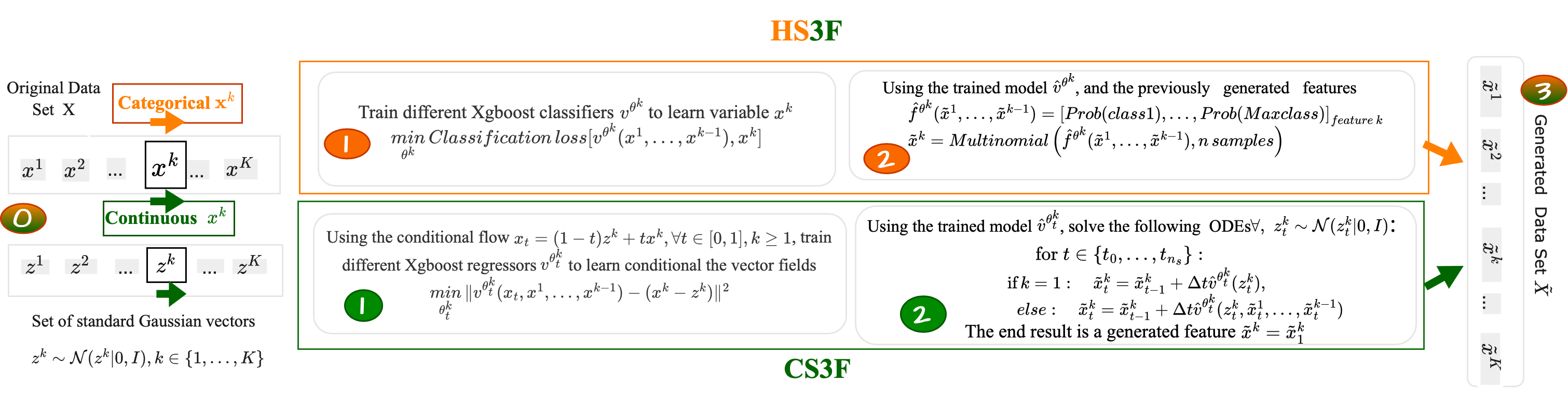
Figure 4: HS3F-based Euler Solver (orange and green rectangle, showing the generation process for both continuous and categorical data) and CS3F-based Euler Solver (encompasses the area inside the green rounded rectangle, showing the continuous data generation). $X=\{x^{1},\dots,x^{K}\}$ is the original data set and $\{z^{1},\dots,z^{K}\}$ is a set containing standard Gaussian feature vectors. The green arrows and steps indicates the generative process continuous features generation while the orange ones indicates that of categorical features. step 0 and 3 contain both colors, which means that both methods use these steps except that the categorical feature generation does not use the set of standard Gaussian noise.

8 Data sets

The data sets Iris and Wine are from scikit-learn and licensed with the BSD 3-Clause License and the remaining are imported from UCI and licensed under the Creative Commons Attribution 4.0 International license (CC BY 4.0). All data sets are openly shared with no restrictions on usage.

Table 5: Dataset Information

Order	Dataset	Reference	Row	Column	Output type
1	Iris	(Fisher, 1988)	150	4	Categorical
2	Wine	(Aeberhard and Forina, 1991)	178	13	Categorical
3	Parkinsons	(Little, 2008)	195	23	Categorical
4	Climate Model Crashes	(Lucas and et al., 2013)	540	18	Categorical
5	Concrete Compression	(Yeh, 2007)	1030	7	Continuous
6	Yacht Hydrodynamics	(Gerritsma and et al., 2013)	308	6	Continuous
7	Airfoil Self Noise	(Brooks et al., 2014)	1503	5	Continuous
8	Connectionist Bench Sonar	(Sejnowski and Gorman, )	208	60	Categorical
9	Ionosphere	(Sigillito et al., 1989)	351	34	Categorical
10	QSAR Biodegradation	(Mansouri et al., 2013)	1055	41	Categorical
11	Seeds	(Charytanowicz, 2012)	210	7	Categorical
12	Glass	(German and Spiehler, 1987)	214	9	Categorical
13	Ecoli	(Nakai, 1996)	336	7	Categorical
14	Yeast	(Nakai, 1996)	1484	8	Categorical
15	Libras	(Dias and et al., 2009)	360	90	Categorical
16	Planning Relax	(Bhatt, 2012)	182	12	Categorical
17	Blood Transfusion	(Yeh, 2008b)	748	4	Categorical
18	Breast Cancer Diagnostic	(Wolberg et al., 1995)	569	30	Categorical
19	Connectionist Bench Vowel	(Deterding, 1997)	990	10	Categorical
20	Concrete Slump	(Yeh, 2009)	103	7	Continuous
21	Wine Quality Red	(Cortez et al., 2009)	1599	10	Continuous
22	Wine Quality White	(Cortez et al., 2009)	4898	11	Continuous
23	Tic-Tac-Toe	(Aha, 1991)	958	9	Categorical
24	Congressional Voting	(UCI Machine Learning Repository, 1987)	435	16	Categorical
25	Car Evaluation	(Bohanec, 1997)	1728	6	Categorical

9 Individual Performance Bar Plots Per Data Set

In this section, we provide the bar plots across all the performance metrics of the methods we used.

9.1 Wasserstein Score

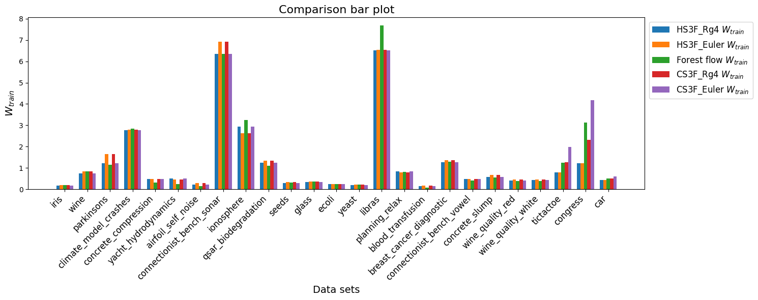
Figure 5: Wasserstein train comparison across datasets

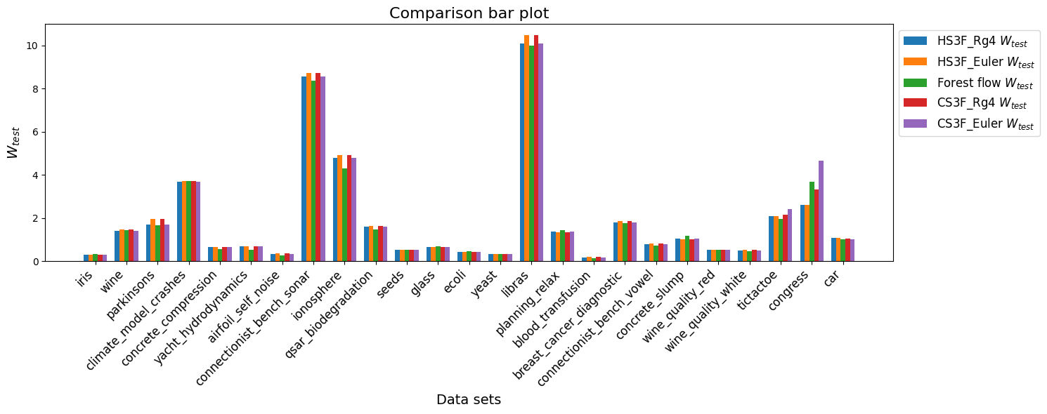
Figure 6: Wasserstein test comparison across generated datasets

9.2 F1 Score

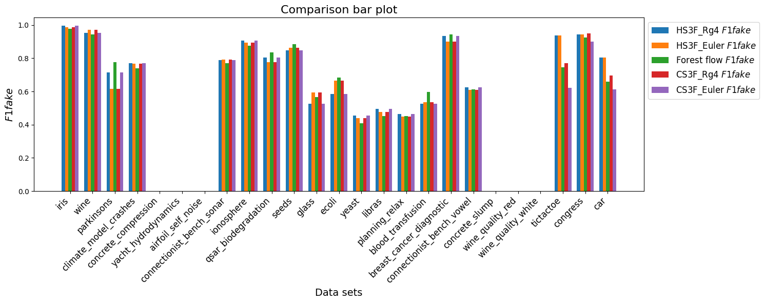
Figure 7: F1 score comparison of models trained on generated datasets

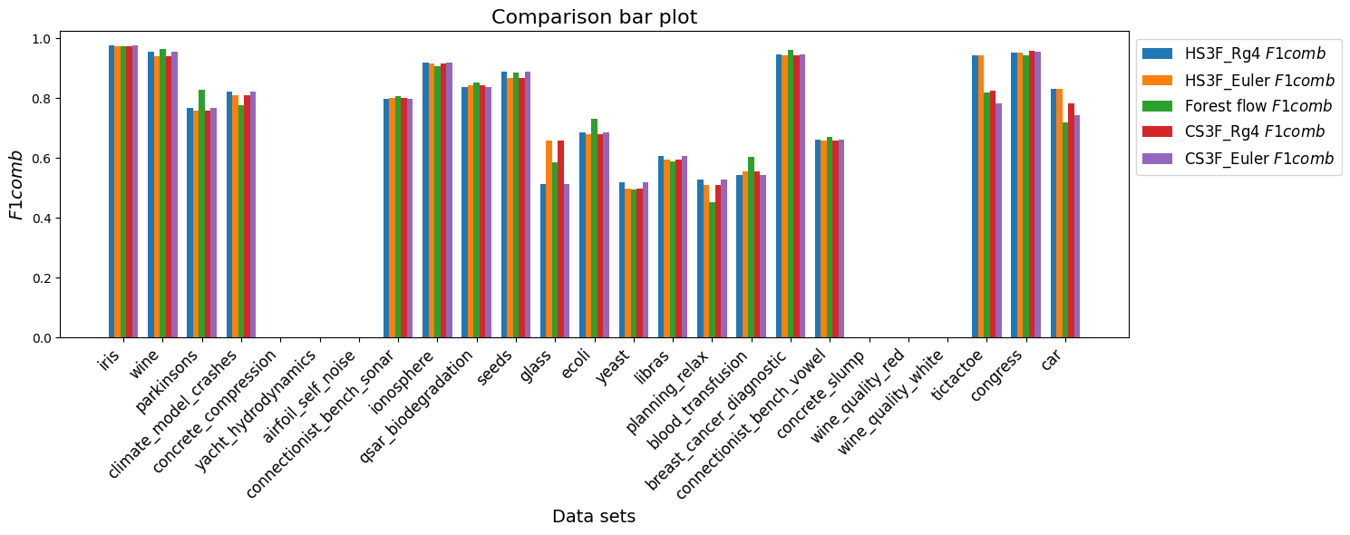
Figure 8: F1 score comparison of models trained on combined datasets (fake+real)

9.3 Coefficient of determination (R2 Squared)

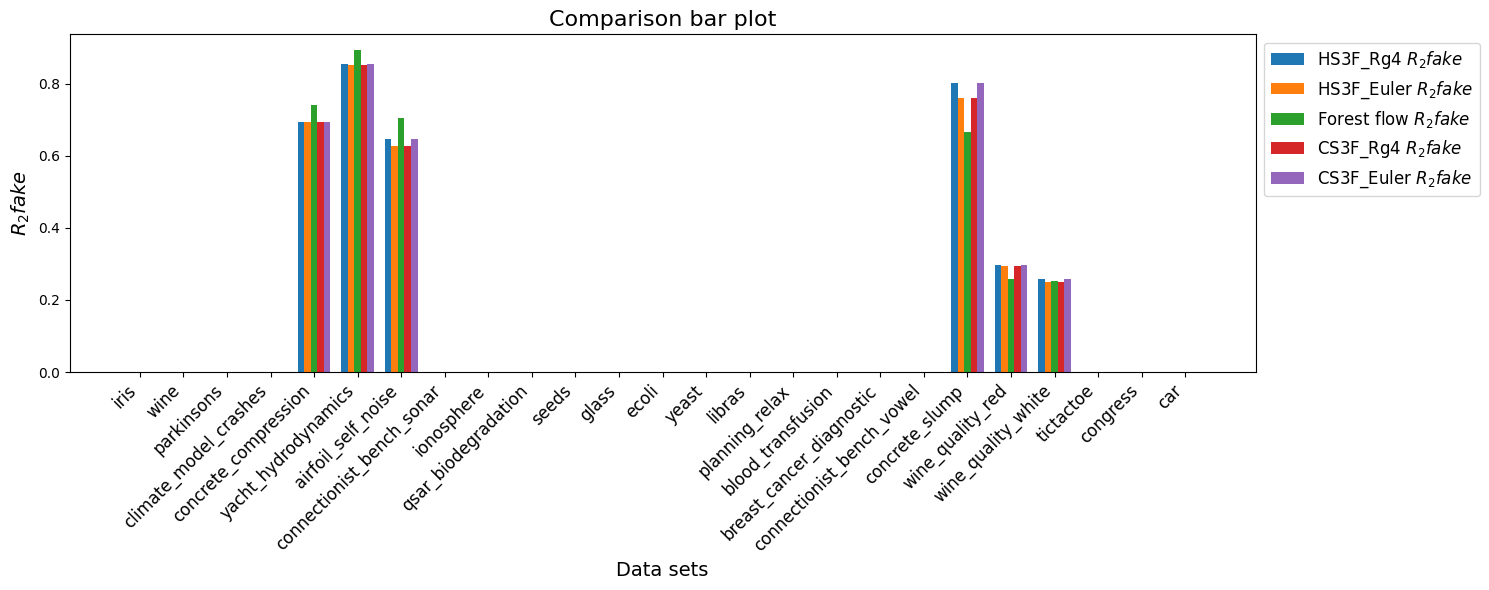
Figure 9: R2 comparison of models trained on generated datasets

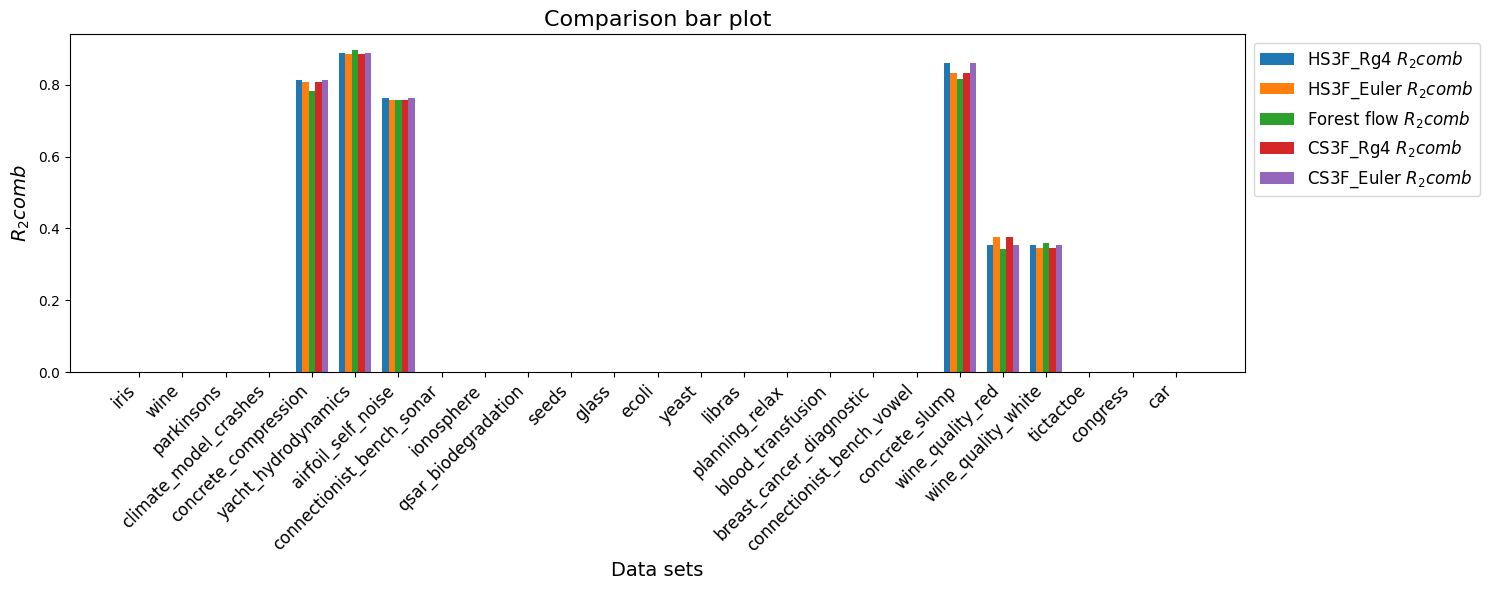
Figure 10: R2 comparison of models trained on combined datasets (fake+real)

9.4 Coverage

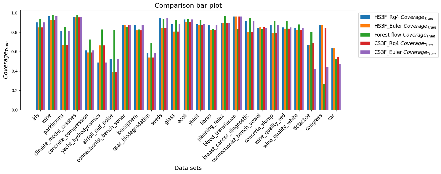
Figure 11: Coverage train comparison across generated datasets

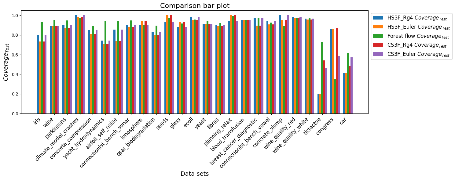
Figure 12: Coverage test comparison across generated datasets

9.5 Data Generation Running Time

Figure 13: Data generation time comparison per models across generated datasets

References

- Aeberhard and Forina (1991) S. Aeberhard and M. Forina. Comparison of methods for classifying between 3 varieties of wine. Data in Brief, 1991.
- Aha (1991) D. W. Aha. Comparing case-based reasoning and other machine learning techniques in tic-tac-toe dataset. Machine Learning Journal, 1991.
- Akinsola (2023) V. Akinsola. Numerical methods: Euler and runge-kutta. In Qualitative and Computational Aspects of Dynamical Systems. IntechOpen, 2023.
- Bhatt (2012) P. Bhatt. A planning relaxation approach for temporal networks. In ICAPS Proceedings, 2012.
- Bohanec (1997) M. Bohanec. Car evaluation. UCI Machine Learning Repository, 10:C5JP48, 1997.
- Borisov et al. (2024) V. Borisov, T. Leemann, K. Seßler, J. Haug, M. Pawelczyk, and G. Kasneci. Deep neural networks and tabular data: A survey. IEEE Transactions on Neural Networks and Learning Systems, 35(6):7499–7519, 2024. doi: 10.1109/TNNLS.2022.3229161.
- Brooks et al. (2014) T. F. Brooks, D. S. Pope, and M. A. Marcolini. Airfoil self-noise and prediction. NASA Technical Report, 2014.
- Charytanowicz (2012) M. Charytanowicz. Assessment of k-means clustering with genetic algorithms for seed dataset. Scientific Research Journal, 2012.
- Chen and Guestrin (2016) T. Chen and C. Guestrin. Xgboost: A scalable tree boosting system. In Proceedings of the 22nd ACM SIGKDD international conference on knowledge discovery and data mining, pages 785–794. ACM, 2016.
- Cortez et al. (2009) P. Cortez et al. Modeling wine preferences by data mining from physicochemical properties. Decision Support Systems, 2009.
- Deterding (1997) P. Deterding. Speaker classification in a vowel recognition benchmark. 1997.
- Dias and et al. (2009) J. Dias and et al. Libras gesture classification: comparing svm, knn and others. Pattern Recognition Letters, 2009.
- Esteban et al. (2017) C. Esteban, S. L. Hyland, and G. Rätsch. Real-valued (medical) time series generation with recurrent conditional gans, 2017.
- Fisher (1988) R. Fisher. The use of multiple measurements in taxonomic problems. Annals of Eugenics, 1988.
- Flamary et al. (2021) R. Flamary, N. Courty, A. Gramfort, M. Z. Alaya, A. Boisbunon, S. Chambon, L. Chapel, A. Corenflos, K. Fatras, N. Fournier, L. Gautheron, N. T. Gayraud, H. Janati, A. Rakotomamonjy, I. Redko, A. Rolet, A. Schutz, V. Seguy, D. J. Sutherland, R. Tavenard, A. Tong, and T. Vayer. Pot: Python optimal transport. Journal of Machine Learning Research, 22(78):1–8, 2021. URL http://jmlr.org/papers/v22/20-451.html.
- German and Spiehler (1987) B. German and V. Spiehler. Glass identification database. UC Irvine Machine Learning Repository, 1987.
- Gerritsma and et al. (2013) M. Gerritsma and et al. Yacht resistance predictions using machine learning. Journal of Fluid Mechanics, 2013.
- Goodfellow et al. (2014) I. Goodfellow, J. Pouget-Abadie, M. Mirza, B. Xu, D. Warde-Farley, S. Ozair, A. Courville, and Y. Bengio. Generative adversarial nets. In Advances in neural information processing systems, pages 2672–2680, 2014.