A Lieb-Robinson bound for open quantum systems with memory
Rahul Trivedi
rahul.trivedi@mpq.mpg.de
Max Planck Institute of Quantum Optics, Garching bei München — 85748, Germany
Mark Rudner
Department Physics, University of Washington, Seattle, WA - 98195, USA
Abstract
We consider a general class of spatially local non-Markovian open quantum lattice models, with a bosonic environment that is approximated as Gaussian. Under the assumption of a finite environment memory time, formalized as a finite total variation of the memory kernel, we show that these models satisfy a Lieb-Robinson bound. Our work generalizes Lieb Robinson bounds for open quantum systems, which have previously only been established in the Markovian limit. Using these bounds, we then show that these non-Markovian models can be well approximated by a larger Markovian model, which contains the system spins together with only a finite number of environment modes. In particular, we establish that as a consequence of our Lieb-Robinson bounds, the number of environment modes per system site needed to accurately capture local observables is independent of the size of the system.
A lattice of quantum spins that only interact with each other locally are physically expected to have only a finite velocity at which correlations can propagate from one spin to another. This qualitative expectation is formalized in the form of Lieb-Robinson bounds [1 ] — given two spatially local operators A 𝐴 A B 𝐵 B [ A ( t ) , B ] 𝐴 𝑡 𝐵 {[A(t),B]} A ( t ) 𝐴 𝑡 A(t) A 𝐴 A t 𝑡 t [2 , 3 ] . Subsequent results relaxed this requirement to exponentially decaying interactions [4 , 5 ] , and more recently, to polynomially decaying interactions [6 , 7 , 8 , 9 , 10 , 11 , 12 , 13 ] .
Lieb-Robinson bounds for lattice Hamiltonians have found an immense number of applications in establishing quasi-locality properties of dynamics [14 , 15 , 16 , 17 ] and characterizing ground state properties for gapped Hamiltonians [17 , 18 , 19 , 20 , 21 , 22 ] , as well as in developing classical and quantum algorithms for simulation of lattice Hamiltonians [23 , 24 ] .
An important question in the study of quantum many-body systems was then to generalize Lieb-Robinson bounds to open quantum systems, where the system evolution cannot be described by a Hamiltonian. Within the Markovian approximation, the open quantum dynamics of a lattice of quantum spins can often be described by a spatially local Lindbladian [25 ] . Lieb Robinson bounds for such models have also been extensively studied — in particular, they have been developed for strictly local Lindbladians [26 , 14 , 27 , 28 ] , as well as Lindbladians with exponentially and polynomially decaying interactions [29 ] . These bounds have subsequently lent rigorous insights into many-body physics of open quantum systems.
In particular, they have been used to study the stability of Lindbladian fixed points [30 , 31 , 32 ] , and developing protocols for simulating open quantum lattice models on both digital quantum computers [28 , 27 ] and analog quantum simulators [33 ] .
However, the existence and nature of Lieb-Robinson bounds for open quantum systems, beyond the Markovian regime, remain important open questions. A key challenge in developing Lieb-Robinson bounds for non-Markovian open quantum systems is the difficulty in describing the reduced system dynamics.
In the Markovian limit, the environment can be traced out to yield a time-local Lindblad master equation for the reduced state of the system.
In the non-Markovian setting, the environment state stores the history of the system, which can in turn influence the system’s evolution [34 , 35 , 36 ] .
Importantly, the environment, which is generally taken to be large, can essentially have an infinite-dimensional Hilbert space and the system-environment interaction Hamiltonian can be unbounded (as for example when the system is coupled to a bosonic field). This creates a significant challenge in obtaining a Lieb-Robinson bound. Indeed, it has been recognized for quite some time that lattice models with infinite local Hilbert space dimension need not even have a Lieb-Robinson bound.
For example, it is possible to construct Hamiltonian lattice models with unbounded local Hilbert space dimension that permit supersonic propagation of correlations [37 ] . In some cases, a Lieb-Robinson bound can be derived despite this issue — in particular, for models of spins interacting with a lattice of linearly coupled bosonic modes [38 ] , as well as for lattice of interacting bosonic modes [39 , 40 , 41 , 42 , 43 ] .
In this paper, we develop a Lieb-Robinson bound for non-Markovian open quantum systems. The only assumption we make on the environment is that it, in the absence of interaction with the system, is non-interacting and can thus be described by a free quantum field. We show that if the environment has finite memory (a notion that we formalize), then the system satisfies a Lieb-Robinson bound with a linear light cone. Equivalently, we establish that the channel on the system generated by the non-Markovian dynamics is quasi-local: in finite-time, it maps local operators to approximately local (or quasi-local) operators.
We next revisit the problem of Markovian dilations of Gaussian non-Markovian environments. For numerical simulations of non-Markovian models, as well as for theoretically characterizing the “amount” of memory that the non-Markovian environment retains of the system, a commonly followed approach is to attempt to approximate the non-Markovian environment by a finite number of bosonic modes [44 , 45 , 46 ] . A standard approach to constructing these bosonic modes is the star-to-chain transformation [45 ] — this transformation has been extensively studied from a theoretical standpoint, and it has been shown that it can well approximate a wide variety of non-Markovian environments [47 , 48 , 49 , 50 ] . However, in current analyses of this transformation the number of environment modes needed to approximate the state of a many-body open quantum system scales polynomially with the system size. For many-body systems that are geometrically local, it can be physically expected that to well approximate only local observables, the number of environment modes per system site needed should be independent of the system size and depend instead only on the evolution time since the local observable dynamics is not expected to depend on the entire many-body system. As an application of the Lieb Robinson bounds that we develop in this paper, we make this qualitative expectation precise.
Figure 1: Schematic depiction of the non-Markovian many-body model considered in this paper. The many-body system is defined on a d − limit-from 𝑑 d- Λ Λ \Lambda R α ν subscript superscript 𝑅 𝜈 𝛼 R^{\nu}_{\alpha} K α ν , ν ′ subscript superscript K 𝜈 superscript 𝜈 ′
𝛼 \textnormal{K}^{\nu,\nu^{\prime}}_{\alpha}
Model . We consider a many-body system of n 𝑛 n d − limit-from 𝑑 d- Λ Λ \Lambda H S ( t ) = ∑ α h α ( t ) subscript 𝐻 S 𝑡 subscript 𝛼 subscript ℎ 𝛼 𝑡 H_{\text{S}}(t)=\sum_{\alpha}h_{\alpha}(t) h α ( t ) subscript ℎ 𝛼 𝑡 h_{\alpha}(t) S α ⊆ Λ subscript 𝑆 𝛼 Λ S_{\alpha}\subseteq\Lambda R α x ( t ) , R α p ( t ) superscript subscript 𝑅 𝛼 𝑥 𝑡 superscript subscript 𝑅 𝛼 𝑝 𝑡
R_{\alpha}^{x}(t),R_{\alpha}^{p}(t) S α subscript 𝑆 𝛼 S_{\alpha} B α , t x , B α , t p subscript superscript 𝐵 𝑥 𝛼 𝑡
subscript superscript 𝐵 𝑝 𝛼 𝑡
B^{x}_{\alpha,t},B^{p}_{\alpha,t} x , p 𝑥 𝑝
x,p α 𝛼 \alpha B α , t x , B α , t p subscript superscript 𝐵 𝑥 𝛼 𝑡
subscript superscript 𝐵 𝑝 𝛼 𝑡
B^{x}_{\alpha,t},B^{p}_{\alpha,t} H SE ( t ) subscript 𝐻 SE 𝑡 H_{\text{SE}}(t)
H SE ( t ) = ∑ α ∑ ν ∈ { x , p } B α , t ν R α ν ( t ) . subscript 𝐻 SE 𝑡 subscript 𝛼 subscript 𝜈 𝑥 𝑝 superscript subscript 𝐵 𝛼 𝑡
𝜈 subscript superscript 𝑅 𝜈 𝛼 𝑡 \displaystyle H_{\text{SE}}(t)=\sum_{\alpha}\sum_{\nu\in\{x,p\}}B_{\alpha,t}^{\nu}R^{\nu}_{\alpha}(t). (1)
Here the time-dependent operators B α , t ν subscript superscript 𝐵 𝜈 𝛼 𝑡
B^{\nu}_{\alpha,t}
H ( t ) = H S ( t ) + H SE ( t ) 𝐻 𝑡 subscript 𝐻 S 𝑡 subscript 𝐻 SE 𝑡 \displaystyle H(t)=H_{\text{S}}(t)+H_{\text{SE}}(t) (2)
Below we will assume that ‖ h α ( t ) ‖ , ‖ R α ν ( t ) ‖ ≤ 1 norm subscript ℎ 𝛼 𝑡 norm superscript subscript 𝑅 𝛼 𝜈 𝑡
1 \left\|{h_{\alpha}(t)}\right\|,\left\|{R_{\alpha}^{\nu}(t)}\right\|\leq 1 ‖ h α ′ ( t ) ‖ , ‖ R α ν ′ ( t ) ‖ < ∞ norm subscript superscript ℎ ′ 𝛼 𝑡 norm superscript superscript subscript 𝑅 𝛼 𝜈 ′ 𝑡
\left\|{h^{\prime}_{\alpha}(t)}\right\|,\left\|{{R_{\alpha}^{\nu}}^{\prime}(t)}\right\|<\infty a 0 subscript 𝑎 0 a_{0} 𝒵 𝒵 \mathcal{Z} diam ( S α ) ≤ a 0 diam subscript 𝑆 𝛼 subscript 𝑎 0 \text{diam}(S_{\alpha})\leq a_{0} S α ′ subscript 𝑆 superscript 𝛼 ′ S_{\alpha^{\prime}} S α subscript 𝑆 𝛼 S_{\alpha} 𝒵 𝒵 \mathcal{Z}
Assuming the environment to initially be in a Gaussian state ρ E subscript 𝜌 𝐸 \rho_{E} t = 0 𝑡 0 t=0
K α ν , ν ′ ( t − t ′ ) = Tr ( B α , t ν B α , t ′ ν ′ ρ E ) , subscript superscript K 𝜈 superscript 𝜈 ′
𝛼 𝑡 superscript 𝑡 ′ Tr subscript superscript 𝐵 𝜈 𝛼 𝑡
subscript superscript 𝐵 superscript 𝜈 ′ 𝛼 superscript 𝑡 ′
subscript 𝜌 𝐸 \displaystyle\text{K}^{\nu,\nu^{\prime}}_{\alpha}(t-t^{\prime})=\text{Tr}(B^{\nu}_{\alpha,t}B^{\nu^{\prime}}_{\alpha,t^{\prime}}\rho_{E}), (3a)
We note that if K α ν , ν ′ ( τ ) ∼ δ ( τ ) similar-to superscript subscript K 𝛼 𝜈 superscript 𝜈 ′
𝜏 𝛿 𝜏 \text{K}_{\alpha}^{\nu,\nu^{\prime}}(\tau)\sim\delta(\tau)
K α ν , ν ′ ( τ ) = K α , c ν , ν ′ ( τ ) + ∑ j k α , j ν , ν ′ δ ( τ − T j ) , subscript superscript K 𝜈 superscript 𝜈 ′
𝛼 𝜏 subscript superscript K 𝜈 superscript 𝜈 ′
𝛼 𝑐
𝜏 subscript 𝑗 superscript subscript 𝑘 𝛼 𝑗
𝜈 superscript 𝜈 ′
𝛿 𝜏 subscript 𝑇 𝑗 \displaystyle\text{K}^{\nu,\nu^{\prime}}_{\alpha}(\tau)=\text{K}^{\nu,\nu^{\prime}}_{\alpha,c}(\tau)+\sum_{j}k_{\alpha,j}^{\nu,\nu^{\prime}}\delta(\tau-T_{j}), (3b)
where K α , c ν , ν ′ subscript superscript K 𝜈 superscript 𝜈 ′
𝛼 𝑐
\text{K}^{\nu,\nu^{\prime}}_{\alpha,c} k α , j ν , ν ′ subscript superscript 𝑘 𝜈 superscript 𝜈 ′
𝛼 𝑗
k^{\nu,\nu^{\prime}}_{\alpha,j}
Several models studied in quantum optics and solid-state physics are captured by Eq. (1 K α ν , ν ′ subscript superscript K 𝜈 superscript 𝜈 ′
𝛼 \text{K}^{\nu,\nu^{\prime}}_{\alpha} δ − limit-from 𝛿 \delta- [51 ] . As another example, models in quantum optics such as lossy Jaynes Cummings models, where the environment can be described by a finite number of lossy bosonic environment modes, admit a similar description [52 , 53 , 54 ] . A bath which has reflections and time-delayed feedback can be described by δ − limit-from 𝛿 \delta- 3b T j subscript 𝑇 𝑗 T_{j} [55 , 56 , 57 ] .
In addition to being physically relevant, the dynamics resulting from the model in Eq. (2 δ − limit-from 𝛿 \delta- K α ν , ν ′ subscript superscript K 𝜈 superscript 𝜈 ′
𝛼 \text{K}^{\nu,\nu^{\prime}}_{\alpha} [48 , 58 ] .
This makes Eq. (2
Lieb Robinson bound . Our first result is to establish a Lieb-Robinson bound for this model. Consider a local obervable O X subscript 𝑂 𝑋 O_{X} X 𝑋 X Λ Λ \Lambda σ S subscript 𝜎 𝑆 \sigma_{S} ρ ( t ′ ) 𝜌 superscript 𝑡 ′ \rho(t^{\prime}) σ S ⊗ ρ E tensor-product subscript 𝜎 𝑆 subscript 𝜌 𝐸 \sigma_{S}\otimes\rho_{E} t ′ superscript 𝑡 ′ t^{\prime} ρ ( t ′ ) = U ( t ′ , 0 ) ( σ S ⊗ ρ E ) U † ( t ′ , 0 ) 𝜌 superscript 𝑡 ′ 𝑈 superscript 𝑡 ′ 0 tensor-product subscript 𝜎 𝑆 subscript 𝜌 𝐸 superscript 𝑈 † superscript 𝑡 ′ 0 \rho(t^{\prime})=U(t^{\prime},0)(\sigma_{S}\otimes\rho_{E})U^{\dagger}(t^{\prime},0) U ( t f , t i ) = 𝒯 exp ( − i ∫ t i t f H ( s ′ ) 𝑑 s ′ ) 𝑈 subscript 𝑡 𝑓 subscript 𝑡 𝑖 𝒯 𝑖 superscript subscript subscript 𝑡 𝑖 subscript 𝑡 𝑓 𝐻 superscript 𝑠 ′ differential-d superscript 𝑠 ′ U(t_{f},t_{i})=\mathcal{T}\exp(-i\int_{t_{i}}^{t_{f}}H(s^{\prime})ds^{\prime}) H ( t ) 𝐻 𝑡 H(t) 2 ρ E subscript 𝜌 𝐸 \rho_{E} ρ ( t ′ ) 𝜌 superscript 𝑡 ′ \rho(t^{\prime})
Next, consider the Heisenberg picture evolution of O X subscript 𝑂 𝑋 O_{X} t ′ superscript 𝑡 ′ t^{\prime} t > t ′ 𝑡 superscript 𝑡 ′ t>t^{\prime} H ( t ) 𝐻 𝑡 H(t) 2 H X [ l ] ( t ) subscript 𝐻 𝑋 delimited-[] 𝑙 𝑡 H_{X[l]}(t) H ( t ) 𝐻 𝑡 H(t) l 𝑙 l X 𝑋 X
H X [ l ] = ∑ α : S α ∩ X [ l ] ≠ ∅ ( h α ( t ) + ∑ ν ∈ { x , p } R α ν ( t ) B ν , t α ) , subscript 𝐻 𝑋 delimited-[] 𝑙 subscript : 𝛼 subscript 𝑆 𝛼 𝑋 delimited-[] 𝑙 subscript ℎ 𝛼 𝑡 subscript 𝜈 𝑥 𝑝 superscript subscript 𝑅 𝛼 𝜈 𝑡 subscript superscript 𝐵 𝛼 𝜈 𝑡
H_{X[l]}=\sum_{\alpha:S_{\alpha}\cap X[l]\neq\emptyset}\bigg{(}h_{\alpha}(t)+\sum_{\nu\in\{x,p\}}R_{\alpha}^{\nu}(t)B^{\alpha}_{\nu,t}\bigg{)},
where X [ l ] 𝑋 delimited-[] 𝑙 X[l] l 𝑙 l X 𝑋 X
( i ) O X ( t , t ′ ) = U † ( t , t ′ ) O X U ( t , t ′ ) , i subscript 𝑂 𝑋 𝑡 superscript 𝑡 ′ superscript 𝑈 † 𝑡 superscript 𝑡 ′ subscript 𝑂 𝑋 𝑈 𝑡 superscript 𝑡 ′ \displaystyle\,(\textrm{i})\ \,O_{X}(t,t^{\prime})=U^{\dagger}(t,t^{\prime})O_{X}U(t,t^{\prime}),
( ii ) O X ( t , t ′ ; l ) = U X [ l ] † ( t , t ′ ) O X U X [ l ] ( t , t ′ ) , ii subscript 𝑂 𝑋 𝑡 superscript 𝑡 ′ 𝑙 superscript subscript 𝑈 𝑋 delimited-[] 𝑙 † 𝑡 superscript 𝑡 ′ subscript 𝑂 𝑋 subscript 𝑈 𝑋 delimited-[] 𝑙 𝑡 superscript 𝑡 ′ \displaystyle(\textrm{ii})\ O_{X}(t,t^{\prime};l)=U_{X[l]}^{\dagger}(t,t^{\prime})O_{X}U_{X[l]}(t,t^{\prime}),
where U X [ l ] ( t f , t i ) = 𝒯 exp ( − i ∫ t i t f H X [ l ] ( s ′ ) 𝑑 s ′ ) subscript 𝑈 𝑋 delimited-[] 𝑙 subscript 𝑡 𝑓 subscript 𝑡 𝑖 𝒯 𝑖 superscript subscript subscript 𝑡 𝑖 subscript 𝑡 𝑓 subscript 𝐻 𝑋 delimited-[] 𝑙 superscript 𝑠 ′ differential-d superscript 𝑠 ′ U_{X[l]}(t_{f},t_{i})=\mathcal{T}\exp(-i\int_{t_{i}}^{t_{f}}H_{X[l]}(s^{\prime})ds^{\prime})
We remark that, had the system-environment Hamiltonian been bounded, then the usual Lieb Robinson bounds for geometrically local lattice Hamiltonians [4 ] would yield that, for sufficiently large l 𝑙 l ‖ O X ( t , t ′ ) − O X ( t , t ′ ; l ) ‖ ≤ e O ( v LR t − l ) norm subscript 𝑂 𝑋 𝑡 superscript 𝑡 ′ subscript 𝑂 𝑋 𝑡 superscript 𝑡 ′ 𝑙 superscript 𝑒 𝑂 subscript 𝑣 LR 𝑡 𝑙 \left\|{O_{X}(t,t^{\prime})-O_{X}(t,t^{\prime};l)}\right\|\leq e^{O(v_{\text{LR}}t-l)} v LR subscript 𝑣 LR v_{\text{LR}} unbounded system-environment Hamiltonian — the interaction terms in the Hamiltonian can be arbitrarily large depending on the system-environment state .
We therefore do not expect such an error bound to hold in general on the operators norm ‖ O X ( t , t ′ ) − O X ( t , t ′ ; l ) ‖ norm subscript 𝑂 𝑋 𝑡 superscript 𝑡 ′ subscript 𝑂 𝑋 𝑡 superscript 𝑡 ′ 𝑙 \left\|{O_{X}(t,t^{\prime})-O_{X}(t,t^{\prime};l)}\right\|
Δ O X ( t , t ′ ; l ) = | Tr ( ( O X ( t , t ′ ) − O X ( t , t ′ ; l ) ) ρ ( t ′ ) ) | , subscript Δ subscript 𝑂 𝑋 𝑡 superscript 𝑡 ′ 𝑙 Tr subscript 𝑂 𝑋 𝑡 superscript 𝑡 ′ subscript 𝑂 𝑋 𝑡 superscript 𝑡 ′ 𝑙 𝜌 superscript 𝑡 ′ \displaystyle\Delta_{O_{X}}(t,t^{\prime};l)=\left|{\textnormal{Tr}\big{(}\big{(}O_{X}(t,t^{\prime})-O_{X}(t,t^{\prime};l)\big{)}\rho(t^{\prime}))}\right|, (4)
characterizing the deviation between the operators O X ( t , t ′ ) subscript 𝑂 𝑋 𝑡 superscript 𝑡 ′ O_{X}(t,t^{\prime}) O X [ l ] ( t , t ′ ; l ) subscript 𝑂 𝑋 delimited-[] 𝑙 𝑡 superscript 𝑡 ′ 𝑙 O_{X[l]}(t,t^{\prime};l) ρ ( t ′ ) 𝜌 superscript 𝑡 ′ \rho(t^{\prime})
Proposition 1 .
Given a local observable O X subscript 𝑂 𝑋 O_{X} X ⊆ Λ 𝑋 Λ X\subseteq\Lambda ∃ v LR > 0 subscript 𝑣 LR 0 \exists\ v_{\textnormal{LR}}>0 σ S subscript 𝜎 𝑆 \sigma_{S} Δ O X ( t , t ′ ; l ) subscript Δ subscript 𝑂 𝑋 𝑡 superscript 𝑡 ′ 𝑙 \Delta_{O_{X}}(t,t^{\prime};l) 4
Δ O X ( t , t ′ ; l ) subscript Δ subscript 𝑂 𝑋 𝑡 superscript 𝑡 ′ 𝑙 \displaystyle\Delta_{O_{X}}(t,t^{\prime};l)
≤ ‖ O X ‖ f ( l ) exp ( − l / a 0 ) ( exp ( v LR | t − t ′ | / a 0 ) − 1 ) , absent norm subscript 𝑂 𝑋 𝑓 𝑙 𝑙 subscript 𝑎 0 subscript 𝑣 LR 𝑡 superscript 𝑡 ′ subscript 𝑎 0 1 \displaystyle\qquad\leq\left\|{O_{X}}\right\|f(l)\exp(-l/a_{0})(\exp(v_{\textnormal{LR}}\left|{t-t^{\prime}}\right|/a_{0})-1),
where, for large l 𝑙 l f ( l ) ≤ O ( l d − 1 ) 𝑓 𝑙 𝑂 superscript 𝑙 𝑑 1 f(l)\leq O(l^{d-1})
Here a 0 subscript 𝑎 0 a_{0} 2 v LR subscript 𝑣 LR v_{\rm LR}
The proof of this proposition departs significantly from the derivation of a Lieb-Robinson bound for finite-dimensional systems due to the infinite-dimensional environment. Additionally, we cannot approximate the environment with a finite-dimensional system by using particle number bounds as was used in Refs. [42 , 43 ] for obtaining a Lieb Robinson bound on the Bose Hubbard model — this is due to the fact that, even with a single excitation in the environment, the system-environment Hamiltonian could still be unbounded due to possible δ − limit-from 𝛿 \delta- ρ S ⊗ ρ E tensor-product subscript 𝜌 𝑆 subscript 𝜌 𝐸 \rho_{S}\otimes\rho_{E} B ν , t α superscript subscript 𝐵 𝜈 𝑡
𝛼 B_{\nu,t}^{\alpha}
Figure 2: Schematic depicting a time-dependent 1D model with supersonic transport that violates a Lieb-Robinson bound with a linear light cone. The model is constructed by interleaving three different time-dependent system-environment Hamiltonians — for 0 ≤ t ≤ 2 T 0 𝑡 2 𝑇 0\leq t\leq 2T T 𝑇 T 2 T ≤ t ≤ 2 T + 1 2 𝑇 𝑡 2 𝑇 1 2T\leq t\leq 2T+1 2 T + 1 ≤ t ≤ 3 T + 1 2 𝑇 1 𝑡 3 𝑇 1 2T+1\leq t\leq 3T+1 T 𝑇 T ∼ T similar-to absent 𝑇 \sim\sqrt{T}
Our analysis also provides us with an explicit expression for a Lieb-Robinson velocity v LR subscript 𝑣 LR v_{\text{LR}}
v LR = e a 0 𝒵 + 56 e a 0 𝒵 TV ( U ) , subscript 𝑣 LR 𝑒 subscript 𝑎 0 𝒵 56 𝑒 subscript 𝑎 0 𝒵 TV U \displaystyle v_{\text{LR}}=ea_{0}\mathcal{Z}+56ea_{0}\mathcal{Z}\textnormal{TV}(\textnormal{U}), (5)
where a 0 , 𝒵 subscript 𝑎 0 𝒵
a_{0},\mathcal{Z} 2 TV ( U ) TV U \text{TV}(\textnormal{U})
TV ( U ) := ∫ − ∞ ∞ U c ( τ ) 𝑑 τ + ∑ j u j , assign TV U superscript subscript subscript U 𝑐 𝜏 differential-d 𝜏 subscript 𝑗 subscript 𝑢 𝑗 \textnormal{TV}(\text{U}):=\int_{-\infty}^{\infty}\text{U}_{c}(\tau)d\tau+\sum_{j}u_{j},
with U ( τ ) = U c ( τ ) + ∑ j = 1 M u j δ ( τ − T j ) U 𝜏 subscript U 𝑐 𝜏 superscript subscript 𝑗 1 𝑀 subscript 𝑢 𝑗 𝛿 𝜏 subscript 𝑇 𝑗 \text{U}(\tau)=\text{U}_{c}(\tau)+\sum_{j=1}^{M}u_{j}\delta(\tau-T_{j}) K α ν , ν ′ superscript subscript K 𝛼 𝜈 superscript 𝜈 ′
\textnormal{K}_{\alpha}^{\nu,\nu^{\prime}}
U c ( τ ) = sup α , ν , ν ′ | K α , c ν , ν ′ ( τ ) | and u j = sup α , ν , ν ′ | k α , j ν , ν ′ | . subscript U 𝑐 𝜏 subscript supremum 𝛼 𝜈 superscript 𝜈 ′
superscript subscript K 𝛼 𝑐
𝜈 superscript 𝜈 ′
𝜏 and subscript 𝑢 𝑗 subscript supremum 𝛼 𝜈 superscript 𝜈 ′
superscript subscript 𝑘 𝛼 𝑗
𝜈 superscript 𝜈 ′
\text{U}_{c}(\tau)=\sup_{\alpha,\nu,\nu^{\prime}}|{\text{K}_{\alpha,c}^{\nu,\nu^{\prime}}(\tau)}|\text{ and }u_{j}=\sup_{\alpha,\nu,\nu^{\prime}}|{k_{\alpha,j}^{\nu,\nu^{\prime}}}|.
Since, by construction, U upper bounds the kernels K α ν , ν ′ superscript subscript K 𝛼 𝜈 superscript 𝜈 ′
\textnormal{K}_{\alpha}^{\nu,\nu^{\prime}} TV ( U ) TV U \text{TV}(\textnormal{U}) TV ( K α ν , ν ′ ) TV superscript subscript K 𝛼 𝜈 superscript 𝜈 ′
\text{TV}(\textnormal{K}_{\alpha}^{\nu,\nu^{\prime}}) K α ν , ν ′ superscript subscript K 𝛼 𝜈 superscript 𝜈 ′
\textnormal{K}_{\alpha}^{\nu,\nu^{\prime}} TV ( U ) TV U \text{TV}(\textnormal{U}) v LR subscript 𝑣 LR v_{\text{LR}}
The dependence of v LR subscript 𝑣 LR v_{\text{LR}} a 0 subscript 𝑎 0 a_{0} S α subscript 𝑆 𝛼 S_{\alpha} 𝒵 𝒵 \mathcal{Z} [26 ] . For the non-Markovian case, v LR subscript 𝑣 LR v_{\text{LR}} U — this can be physically interpreted as a measure of the memory effects in the environment and of the extent to which system state can be time-correlated with its past. With this interpretation, this dependence of v LR subscript 𝑣 LR v_{\text{LR}} TV ( U ) TV U \textnormal{TV}(\text{U})
The discussion above indicates that, for
TV ( U ) → ∞ → TV U \textnormal{TV}(\text{U})\to\infty 1 v LR subscript 𝑣 LR v_{\rm LR} 5 t 𝑡 t ∝ t α proportional-to absent superscript 𝑡 𝛼 \propto t^{\alpha} α > 1 𝛼 1 \alpha>1 [37 ] , which also developed a lattice of infinite-dimensional systems with supersonic transport, in that we explicitly consider models that have a Hamiltonian of the form in Eq. 2 [37 ] required more complex nearest neighbour interactions and didnt satisfy Eq. 2 N 𝑁 N 2 N 𝑁 N a 1 , a 2 … a N subscript 𝑎 1 subscript 𝑎 2 … subscript 𝑎 𝑁
a_{1},a_{2}\dots a_{N} B α , t ν subscript superscript 𝐵 𝜈 𝛼 𝑡
B^{\nu}_{\alpha,t} 1 B α , t x = ( a α + a α † ) / 2 subscript superscript 𝐵 𝑥 𝛼 𝑡
subscript 𝑎 𝛼 superscript subscript 𝑎 𝛼 † 2 B^{x}_{\alpha,t}=(a_{\alpha}+a_{\alpha}^{\dagger})/\sqrt{2} B α , t p = ( a α − a α † ) / 2 i subscript superscript 𝐵 𝑝 𝛼 𝑡
subscript 𝑎 𝛼 superscript subscript 𝑎 𝛼 † 2 𝑖 B^{p}_{\alpha,t}=(a_{\alpha}-a_{\alpha}^{\dagger})/\sqrt{2}i | K α ν , ν ′ ( t ) | = 1 / 2 for any t subscript superscript K 𝜈 superscript 𝜈 ′
𝛼 𝑡 1 2 for any 𝑡 |{\textnormal{K}^{\nu,\nu^{\prime}}_{\alpha}(t)}|=1/2\text{ for any }t
To achieve supersonic transport in this model, we
consider a total evolution time of 3 T + 1 3 𝑇 1 3T+1 T = m 2 𝑇 superscript 𝑚 2 T=m^{2} m > 0 𝑚 0 m>0 T 𝑇 T 2 T 2 𝑇 2T t = 0 𝑡 0 t=0 t = 2 T 𝑡 2 𝑇 t=2T | 0 ⟩ → | 1 ⟩ → ket 0 ket 1 \ket{0}\to\ket{1} π 𝜋 \pi H S = π 2 σ x subscript 𝐻 S 𝜋 2 subscript 𝜎 𝑥 H_{\rm S}=\frac{\pi}{2}\sigma_{x} H SE = h JC = π 2 ( σ † a + h.c. ) subscript 𝐻 SE subscript ℎ JC 𝜋 2 superscript 𝜎 † 𝑎 h.c. H_{\rm SE}=h_{\text{JC}}=\frac{\pi}{2}(\sigma^{\dagger}a+\text{h.c.}) T 𝑇 T | 0 ⟩ ket 0 \ket{0} 2 T 2 𝑇 2T 2 T + 1 2 𝑇 1 2T+1 | 0 ⟩ → | 1 ⟩ → ket 0 ket 1 \ket{0}\to\ket{1} σ 1 † | 0 ⟩ ⊗ n ⊗ | T ⟩ ⊗ n tensor-product superscript subscript 𝜎 1 † superscript ket 0 tensor-product absent 𝑛 superscript ket 𝑇 tensor-product absent 𝑛 \sigma_{1}^{\dagger}\ket{0}^{\otimes n}\otimes\ket{T}^{\otimes n} 2 T + 1 2 𝑇 1 2T+1 3 T + 1 3 𝑇 1 3T+1 T 𝑇 T T T 𝑇 𝑇 T\sqrt{T} h JC 2 Q = π 2 ( | 01 ⟩ ⟨ 10 | a + h.c. ) subscript superscript ℎ 2 𝑄 JC 𝜋 2 ket 01 bra 10 𝑎 h.c. h^{2Q}_{\text{JC}}=\frac{\pi}{2}(\ket{01}\!\bra{10}a+\text{h.c.}) | 10 ⟩ ⊗ | T ⟩ → | 01 ⟩ ⊗ | T − 1 ⟩ → tensor-product ket 10 ket 𝑇 tensor-product ket 01 ket 𝑇 1 \ket{10}\otimes\ket{T}\to\ket{01}\otimes\ket{T-1} 1 / T 1 𝑇 1/\sqrt{T} 1 / T 1 𝑇 1/\sqrt{T} 1 / T 1 𝑇 1/\sqrt{T} 2 2 2 3 3 3 3 T + 1 3 𝑇 1 3T+1 σ T T + 1 † | 0 ⟩ ⊗ n superscript subscript 𝜎 𝑇 𝑇 1 † superscript ket 0 tensor-product absent 𝑛 \sigma_{T\sqrt{T}+1}^{\dagger}\ket{0}^{\otimes n} supersonic transport of the excitation at the first qubit across a distance T T 𝑇 𝑇 T\sqrt{T} T 𝑇 T
We remark that all the time-dependent terms in the system-environment Hamiltonian can be switched on and off smoothly to ensure that they are differentiable with respect to time as required in our setup [see text below Eq. (1 σ T m + 1 † σ T m + 1 superscript subscript 𝜎 𝑇 𝑚 1 † subscript 𝜎 𝑇 𝑚 1 \sigma_{Tm+1}^{\dagger}\sigma_{Tm+1} ( T m + 1 ) th superscript 𝑇 𝑚 1 th (Tm+1)^{\text{th}} Δ σ T m + 1 † σ T m + 1 ( 3 T + 1 , 0 ; l ) subscript Δ superscript subscript 𝜎 𝑇 𝑚 1 † subscript 𝜎 𝑇 𝑚 1 3 𝑇 1 0 𝑙 \Delta_{\sigma_{Tm+1}^{\dagger}\sigma_{Tm+1}}(3T+1,0;l) 4 l < T T + 1 𝑙 𝑇 𝑇 1 l<T\sqrt{T+1}
Implication on bath approximations . Next, we consider the problem of approximating the non-Markovian environment with a finite number of bosonic modes per site.
For a many-body system, if we are interested in approximating the full system state at a given time and to a target precision then the number of modes in the environment is expected to scale with the system size since we effectively demand a high precision on high-order correlators in the system. However, for a geometrically local many-body system interacting locally with independent baths, it is physically expected that local observables or few-point correlation functions in the system can be approximated well by a number of modes in each local bath that is independent of the system size, and depends only on the evolution time and the target precision.
Figure 3: Schematic depiction of the star-to-chain transformation used to approximate a non-Markovian environment by a discrete set of bosonic modes. Each bath is replaced with N m subscript 𝑁 𝑚 N_{m} N m subscript 𝑁 𝑚 N_{m}
This physical expectation can be made precise by applying the Lieb Robinson bounds from Proposition 1. We will analyze the star-to-chain transformation as the method to construct the discrete-mode approximation of each bath [45 , 49 , 48 ] .
As depicted in Fig. 3 N m subscript 𝑁 𝑚 N_{m} N m subscript 𝑁 𝑚 N_{m} b α , 1 , b α , 2 … b α , N m subscript 𝑏 𝛼 1
subscript 𝑏 𝛼 2
… subscript 𝑏 𝛼 subscript 𝑁 𝑚
b_{\alpha,1},b_{\alpha,2}\dots b_{\alpha,N_{m}} 1
H SE N m ( t ) = ∑ α [ g α x α , 1 ( t ) R α x ( t ) + g α p α , 1 ( t ) R α p ( t ) ] , superscript subscript 𝐻 SE subscript 𝑁 𝑚 𝑡 subscript 𝛼 delimited-[] subscript 𝑔 𝛼 subscript 𝑥 𝛼 1
𝑡 superscript subscript 𝑅 𝛼 𝑥 𝑡 subscript 𝑔 𝛼 subscript 𝑝 𝛼 1
𝑡 superscript subscript 𝑅 𝛼 𝑝 𝑡 {H}_{\text{SE}}^{N_{m}}(t)=\sum_{\alpha}\left[g_{\alpha}x_{\alpha,1}(t)R_{\alpha}^{x}(t)+g_{\alpha}p_{\alpha,1}(t)R_{\alpha}^{p}(t)\right],
where x α , 1 ( t ) = ( b α , 1 ( t ) + b α , 1 † ( t ) ) / 2 subscript 𝑥 𝛼 1
𝑡 subscript 𝑏 𝛼 1
𝑡 superscript subscript 𝑏 𝛼 1
† 𝑡 2 x_{\alpha,1}(t)=(b_{\alpha,1}(t)+b_{\alpha,1}^{\dagger}(t))/\sqrt{2} p α , 1 = ( b α , 1 ( t ) − b α , 1 † ( t ) ) / 2 i subscript 𝑝 𝛼 1
subscript 𝑏 𝛼 1
𝑡 superscript subscript 𝑏 𝛼 1
† 𝑡 2 𝑖 p_{\alpha,1}=(b_{\alpha,1}(t)-b_{\alpha,1}^{\dagger}(t))/\sqrt{2}i b α , 1 ( t ) = e i H α , E t b α , 1 e − i H α , E t subscript 𝑏 𝛼 1
𝑡 superscript 𝑒 𝑖 subscript 𝐻 𝛼 𝐸
𝑡 subscript 𝑏 𝛼 1
superscript 𝑒 𝑖 subscript 𝐻 𝛼 𝐸
𝑡 b_{\alpha,1}(t)=e^{iH_{\alpha,E}t}b_{\alpha,1}e^{-iH_{\alpha,E}t}
H α , E = ∑ j = 1 N m ω α , j b α , j † b α , j + ∑ j = 1 N m − 1 ( t α , j b α , j † b α , j + 1 + h.c. ) . subscript 𝐻 𝛼 𝐸
superscript subscript 𝑗 1 subscript 𝑁 𝑚 subscript 𝜔 𝛼 𝑗
superscript subscript 𝑏 𝛼 𝑗
† subscript 𝑏 𝛼 𝑗
superscript subscript 𝑗 1 subscript 𝑁 𝑚 1 subscript 𝑡 𝛼 𝑗
superscript subscript 𝑏 𝛼 𝑗
† subscript 𝑏 𝛼 𝑗 1
h.c. H_{\alpha,E}=\sum_{j=1}^{N_{m}}\omega_{\alpha,j}b_{\alpha,j}^{\dagger}b_{\alpha,j}+\sum_{j=1}^{N_{m}-1}\big{(}t_{\alpha,j}b_{\alpha,j}^{\dagger}b_{\alpha,j+1}+\text{h.c.}\big{)}.
The constants g α , ω α , j , t α , j subscript 𝑔 𝛼 subscript 𝜔 𝛼 𝑗
subscript 𝑡 𝛼 𝑗
g_{\alpha},\omega_{\alpha,j},t_{\alpha,j} H SE ( t ) subscript 𝐻 SE 𝑡 H_{\text{SE}}(t) H SE N m ( t ) subscript superscript 𝐻 subscript 𝑁 𝑚 SE 𝑡 H^{N_{m}}_{\text{SE}}(t) K α ν , ν ′ ( t ) superscript subscript K 𝛼 𝜈 superscript 𝜈 ′
𝑡 \text{K}_{\alpha}^{\nu,\nu^{\prime}}(t) 3a
Employing the Lieb-Robinson bounds from Proposition 1, we now estimate the number of modes N m subscript 𝑁 𝑚 N_{m} N m subscript 𝑁 𝑚 N_{m}
Proposition 2 .
There exists an approximation of the non-Markovian environment with N m subscript 𝑁 𝑚 N_{m} O 𝑂 O O ( 1 ) 𝑂 1 O(1) ‖ O ‖ ≤ 1 norm 𝑂 1 \left\|{O}\right\|\leq 1 ε 𝜀 \varepsilon t 𝑡 t
N m subscript 𝑁 𝑚 \displaystyle N_{m} = Θ ( ( ε − 1 t 2 d + 3 ) 1 + o ( 1 ) ) + Θ ( ( ε − 1 log ε − 1 ) 1 + o ( 1 ) ) + + \displaystyle=\Theta\big{(}\big{(}\varepsilon^{-1}{t^{2d+3}}\big{)}^{1+o(1)}\big{)}+\Theta\big{(}\big{(}{\varepsilon}^{-1}\log\varepsilon^{-1}\big{)}^{1+o(1)}\big{)}++
Θ ( ( t κ 0 ( ε − 1 Θ ( t d + 1 ) Θ ( t log d ε − 1 ) ) 1 + o ( 1 ) ) , \displaystyle\qquad\Theta\big{(}\big{(}t\kappa_{0}\big{(}\varepsilon^{-1}\Theta(t^{d+1})\Theta(t\log^{d}\varepsilon^{-1})\big{)}^{1+o(1)}\big{)},
where κ 0 : ( 0 , ∞ ) → ( 0 , ∞ ) : subscript 𝜅 0 → 0 0 \kappa_{0}:(0,\infty)\to(0,\infty)
1 x = ∑ τ ∈ { 0 , t } ∫ τ − κ 0 ( x ) τ + κ 0 ( x ) U c ( s ) 𝑑 s . 1 𝑥 subscript 𝜏 0 𝑡 superscript subscript 𝜏 subscript 𝜅 0 𝑥 𝜏 subscript 𝜅 0 𝑥 subscript U 𝑐 𝑠 differential-d 𝑠 \frac{1}{x}=\sum_{\tau\in\{0,t\}}\int_{\tau-\kappa_{0}(x)}^{\tau+\kappa_{0}(x)}\textnormal{U}_{c}(s)ds.
The proof of this proposition follows almost directly from Proposition 1 — the evolution of the local observable upto time t 𝑡 t O ( t ) 𝑂 𝑡 O(t) [49 , 48 ] . The details of our analyses can be found in the supplementary material. While we have chosen to analyze the star-to-chain transformation, we expect a similar conclusion to hold for other methods for approximating the bath, such as the pseudo-mode approximation, which could outperform the star-to-chain transformation for specific systems [44 , 46 ] .
Conclusion . Our work provides a Lieb-Robinson bound for non-Markovian many-body systems, which fundamentally provides a velocity of propagation of information in these systems. Similar to the Markovian case, we expect this bound to be important in a theoretical study of both non-equilibrium as well equilibrium properties of non-Markovian many-body systems.
Our work opens up several interesting questions pertaining to non-Markovian many-body physics, as well as provides techincal tools that could possibly be developed further to answering these questions. Since we are considering non-Markovian models, in comparison to the Markovian case, there is a possibility of creating interactions between the qubits, via the environment, that are correlated in time and not just in space. The first open question is to more sharply understand propagation of information in non-Markovian models where the kernels decay slowly and algebraically and thus have an infinite total variation (e.g., if the kernels ∼ t − α similar-to absent superscript 𝑡 𝛼 \sim t^{-\alpha} α ∈ ( 0 , 1 ) 𝛼 0 1 \alpha\in(0,1)
References
[1]
C.-F. A. Chen, A. Lucas, and C. Yin, “Speed limits and locality in many-body
quantum dynamics,” Reports on Progress in Physics , vol. 86, no. 11,
p. 116001, 2023.
[2]
E. H. Lieb and D. W. Robinson, “The finite group velocity of quantum spin
systems,” Communications in mathematical physics , vol. 28, no. 3,
pp. 251–257, 1972.
[3]
M. B. Hastings, “Lieb-schultz-mattis in higher dimensions,” Physical
review b , vol. 69, no. 10, p. 104431, 2004.
[4]
M. B. Hastings and T. Koma, “Spectral gap and exponential decay of
correlations,” Communications in mathematical physics , vol. 265,
pp. 781–804, 2006.
[5]
B. Nachtergaele and R. Sims, “Lieb-robinson bounds and the exponential
clustering theorem,” Communications in mathematical physics , vol. 265,
pp. 119–130, 2006.
[6]
C.-F. Chen and A. Lucas, “Finite speed of quantum scrambling with long range
interactions,” Physical review letters , vol. 123, no. 25, p. 250605,
2019.
[7]
C.-F. Chen and A. Lucas, “Optimal frobenius light cone in spin chains with
power-law interactions,” Physical Review A , vol. 104, no. 6,
p. 062420, 2021.
[8]
M. Foss-Feig, Z.-X. Gong, C. W. Clark, and A. V. Gorshkov, “Nearly linear
light cones in long-range interacting quantum systems,” Physical review
letters , vol. 114, no. 15, p. 157201, 2015.
[9]
D. V. Else, F. Machado, C. Nayak, and N. Y. Yao, “Improved lieb-robinson bound
for many-body hamiltonians with power-law interactions,” Physical
Review A , vol. 101, no. 2, p. 022333, 2020.
[10]
Z. Eldredge, Z.-X. Gong, J. T. Young, A. H. Moosavian, M. Foss-Feig, and A. V.
Gorshkov, “Fast quantum state transfer and entanglement renormalization
using long-range interactions,” Physical review letters , vol. 119,
no. 17, p. 170503, 2017.
[11]
M. C. Tran, C.-F. Chen, A. Ehrenberg, A. Y. Guo, A. Deshpande, Y. Hong, Z.-X.
Gong, A. V. Gorshkov, and A. Lucas, “Hierarchy of linear light cones with
long-range interactions,” Physical Review X , vol. 10, no. 3,
p. 031009, 2020.
[12]
M. C. Tran, A. Y. Guo, A. Deshpande, A. Lucas, and A. V. Gorshkov, “Optimal
state transfer and entanglement generation in power-law interacting
systems,” Physical Review X , vol. 11, no. 3, p. 031016, 2021.
[13]
Y. Hong and A. Lucas, “Fast high-fidelity multiqubit state transfer with
long-range interactions,” Physical Review A , vol. 103, no. 4,
p. 042425, 2021.
[14]
M. Kliesch, C. Gogolin, and J. Eisert, “Lieb-robinson bounds and the
simulation of time-evolution of local observables in lattice systems,” Many-Electron Approaches in Physics, Chemistry and Mathematics: A
Multidisciplinary View , pp. 301–318, 2014.
[15]
T. J. Osborne, “Efficient approximation of the dynamics of one-dimensional
quantum spin systems,” Physical review letters , vol. 97, no. 15,
p. 157202, 2006.
[16]
S. Bravyi, M. B. Hastings, and F. Verstraete, “Lieb-robinson bounds and the
generation of correlations and topological quantum order,” Physical
review letters , vol. 97, no. 5, p. 050401, 2006.
[17]
M. B. Hastings, “Locality in quantum and markov dynamics on lattices and
networks,” Physical review letters , vol. 93, no. 14, p. 140402, 2004.
[18]
M. B. Hastings, “An area law for one-dimensional quantum systems,” Journal of statistical mechanics: theory and experiment , vol. 2007, no. 08,
p. P08024, 2007.
[19]
M. B. Hastings and X.-G. Wen, “Quasiadiabatic continuation of quantum states:
The stability of topological ground-state degeneracy and emergent gauge
invariance,” Physical Review B—Condensed Matter and Materials
Physics , vol. 72, no. 4, p. 045141, 2005.
[20]
M. B. Hastings, “Quasi-adiabatic continuation for disordered systems:
Applications to correlations, lieb-schultz-mattis, and hall conductance,”
arXiv preprint arXiv:1001.5280 , 2010.
[21]
M. B. Hastings, “Gapped quantum systems: From higher dimensional
lieb-schultz-mattis to the quantum hall effect,” arXiv preprint
arXiv:2111.01854 , 2021.
[22]
B. Nachtergaele, R. Sims, and A. Young, “Quasi-locality bounds for quantum
lattice systems. i. lieb-robinson bounds, quasi-local maps, and spectral flow
automorphisms,” Journal of Mathematical Physics , vol. 60, no. 6, 2019.
[23]
J. Haah, M. B. Hastings, R. Kothari, and G. H. Low, “Quantum algorithm for
simulating real time evolution of lattice hamiltonians,” SIAM Journal
on Computing , vol. 52, no. 6, pp. FOCS18–250, 2021.
[24]
M. C. Tran, A. Y. Guo, Y. Su, J. R. Garrison, Z. Eldredge, M. Foss-Feig, A. M.
Childs, and A. V. Gorshkov, “Locality and digital quantum simulation of
power-law interactions,” Physical Review X , vol. 9, no. 3, p. 031006,
2019.
[25]
H.-P. Breuer and F. Petruccione, The theory of open quantum systems .
Oxford University Press, USA, 2002.
[26]
D. Poulin, “Lieb-robinson bound and locality for general markovian quantum
dynamics,” Physical review letters , vol. 104, no. 19, p. 190401, 2010.
[27]
T. Barthel and M. Kliesch, “Quasilocality and efficient simulation of
markovian quantum dynamics,” Physical review letters , vol. 108,
no. 23, p. 230504, 2012.
[28]
M. Kliesch, T. Barthel, C. Gogolin, M. Kastoryano, and J. Eisert, “Dissipative
quantum church-turing theorem,” Physical review letters , vol. 107,
no. 12, p. 120501, 2011.
[29]
R. Sweke, J. Eisert, and M. Kastner, “Lieb–robinson bounds for open quantum
systems with long-ranged interactions,” Journal of Physics A:
Mathematical and Theoretical , vol. 52, no. 42, p. 424003, 2019.
[30]
A. Lucia, T. S. Cubitt, S. Michalakis, and D. Pérez-García, “Rapid
mixing and stability of quantum dissipative systems,” Physical Review
A , vol. 91, no. 4, p. 040302, 2015.
[31]
T. S. Cubitt, A. Lucia, S. Michalakis, and D. Perez-Garcia, “Stability of
local quantum dissipative systems,” Communications in Mathematical
Physics , vol. 337, pp. 1275–1315, 2015.
[32]
F. G. Brandao, T. S. Cubitt, A. Lucia, S. Michalakis, and D. Perez-Garcia,
“Area law for fixed points of rapidly mixing dissipative quantum systems,”
Journal of mathematical physics , vol. 56, no. 10, 2015.
[33]
V. Kashyap, G. Styliaris, S. Mouradian, J. I. Cirac, and R. Trivedi, “Accuracy
guarantees and quantum advantage in analogue open quantum simulation with and
without noise,” arXiv preprint arXiv:2404.11081 , 2024.
[34]
I. De Vega and D. Alonso, “Dynamics of non-markovian open quantum systems,”
Reviews of Modern Physics , vol. 89, no. 1, p. 015001, 2017.
[35]
H.-P. Breuer, E.-M. Laine, J. Piilo, and B. Vacchini, “Colloquium:
Non-markovian dynamics in open quantum systems,” Reviews of Modern
Physics , vol. 88, no. 2, p. 021002, 2016.
[36]
D. Gribben, A. Strathearn, G. E. Fux, P. Kirton, and B. W. Lovett, “Using the
environment to understand non-markovian open quantum systems,” Quantum , vol. 6, p. 847, 2022.
[37]
J. Eisert and D. Gross, “Supersonic quantum communication,” Physical
review letters , vol. 102, no. 24, p. 240501, 2009.
[38]
J. Jünemann, A. Cadarso, D. Pérez-García, A. Bermudez, and J. J.
García-Ripoll, “Lieb-robinson bounds for spin-boson lattice models and
trapped ions,” Physical review letters , vol. 111, no. 23, p. 230404,
2013.
[39]
N. Schuch, S. K. Harrison, T. J. Osborne, and J. Eisert, “Information
propagation for interacting-particle systems,” Physical Review
A—Atomic, Molecular, and Optical Physics , vol. 84, no. 3, p. 032309, 2011.
[40]
T. Kuwahara and K. Saito, “Lieb-robinson bound and almost-linear light cone in
interacting boson systems,” Physical review letters , vol. 127, no. 7,
p. 070403, 2021.
[41]
H. Raz and R. Sims, “Estimating the lieb-robinson velocity for classical
anharmonic lattice systems,” Journal of Statistical Physics , vol. 137,
pp. 79–108, 2009.
[42]
C. Yin and A. Lucas, “Finite speed of quantum information in models of
interacting bosons at finite density,” Physical Review X , vol. 12,
no. 2, p. 021039, 2022.
[43]
T. Kuwahara, T. V. Vu, and K. Saito, “Effective light cone and digital quantum
simulation of interacting bosons,” Nature Communications , vol. 15,
no. 1, p. 2520, 2024.
[44]
D. Tamascelli, A. Smirne, S. F. Huelga, and M. B. Plenio, “Nonperturbative
treatment of non-markovian dynamics of open quantum systems,” Physical
review letters , vol. 120, no. 3, p. 030402, 2018.
[45]
A. W. Chin, Á. Rivas, S. F. Huelga, and M. B. Plenio, “Exact mapping
between system-reservoir quantum models and semi-infinite discrete chains
using orthogonal polynomials,” Journal of Mathematical Physics ,
vol. 51, no. 9, 2010.
[46]
G. Pleasance, B. M. Garraway, and F. Petruccione, “Generalized theory of
pseudomodes for exact descriptions of non-markovian quantum processes,” Physical Review Research , vol. 2, no. 4, p. 043058, 2020.
[47]
R. Trivedi, D. Malz, and J. I. Cirac, “Convergence guarantees for discrete
mode approximations to non-markovian quantum baths,” Physical review
letters , vol. 127, no. 25, p. 250404, 2021.
[48]
R. Trivedi, “Description and complexity of non-markovian open quantum
dynamics,” arXiv preprint arXiv:2204.06936 , 2022.
[49]
M. P. Woods, M. Cramer, and M. B. Plenio, “Simulating bosonic baths with error
bars,” Physical Review Letters , vol. 115, no. 13, p. 130401, 2015.
[50]
F. Mascherpa, A. Smirne, S. F. Huelga, and M. B. Plenio, “Open systems with
error bounds: spin-boson model with spectral density variations,” Physical review letters , vol. 118, no. 10, p. 100401, 2017.
[51]
T. Shi, Y.-H. Wu, A. González-Tudela, and J. I. Cirac, “Bound states in
boson impurity models,” Physical Review X , vol. 6, no. 2, p. 021027,
2016.
[52]
L. Mazzola, S. Maniscalco, J. Piilo, K.-A. Suominen, and B. M. Garraway,
“Pseudomodes as an effective description of memory: Non-markovian dynamics
of two-state systems in structured reservoirs,” Physical Review
A—Atomic, Molecular, and Optical Physics , vol. 80, no. 1, p. 012104, 2009.
[53]
B. Dalton, S. M. Barnett, and B. M. Garraway, “Theory of pseudomodes in
quantum optical processes,” Physical Review A , vol. 64, no. 5,
p. 053813, 2001.
[54]
B. M. Garraway and B. Dalton, “Theory of non-markovian decay of a cascade atom
in high-q cavities and photonic band gap materials,” Journal of Physics
B: Atomic, Molecular and Optical Physics , vol. 39, no. 15, p. S767, 2006.
[55]
A. L. Grimsmo, “Time-delayed quantum feedback control,” Physical review
letters , vol. 115, no. 6, p. 060402, 2015.
[56]
S. Whalen, A. Grimsmo, and H. Carmichael, “Open quantum systems with delayed
coherent feedback,” Quantum Science and Technology , vol. 2, no. 4,
p. 044008, 2017.
[57]
H. Pichler and P. Zoller, “Photonic circuits with time delays and quantum
feedback,” Physical review letters , vol. 116, no. 9, p. 093601, 2016.
[58]
D. Lonigro, “Generalized spin-boson models with non-normalizable form
factors,” Journal of Mathematical Physics , vol. 63, no. 7, 2022.
[59]
B. Mollow, “Pure-state analysis of resonant light scattering: Radiative
damping, saturation, and multiphoton effects,” Physical Review A ,
vol. 12, no. 5, p. 1919, 1975.
[60]
C. W. Gardiner and M. J. Collett, “Input and output in damped quantum systems:
Quantum stochastic differential equations and the master equation,” Physical Review A , vol. 31, no. 6, p. 3761, 1985.
[61]
K. R. Parthasarathy, An introduction to quantum stochastic calculus ,
vol. 85.
Birkhäuser, 2012.
[62]
A. Israel, “The eigenvalue distribution of time-frequency localization
operators,” arXiv preprint arXiv:1502.04404 , 2015.
Supplementary Information
Contents
I Notation
II Preliminaries
II.1 SetupII.2 Wick’s theoremII.3 Analyzing the mollification
III The Lieb Robinson Bound
III.1 Reviewing the Lieb-Robinson bound for bounded lattice HamiltoniansIII.2 Identifying operator spacesIII.3 Defining the commutator boundIII.4 Deriving the Lieb-Robinson bound (Proof of proposition 1)
IV Violation the linear light-cone
V Markovian Dilations for local observables
V.1 PreliminariesV.2 Analyzing error in star-to-chain transformationV.3 Proof of proposition 2
I Notation
Given a Hilbert space ℋ ℋ \mathcal{H} L ( ℋ ) L ℋ \text{L}(\mathcal{H}) ℋ → ℋ → ℋ ℋ \mathcal{H}\to\mathcal{H} M ( ℋ ) M ℋ \text{M}(\mathcal{H}) ℋ → ℋ → ℋ ℋ \mathcal{H}\to\mathcal{H} D 1 ( ℋ ) subscript D 1 ℋ \text{D}_{1}(\mathcal{H}) ℋ ℋ \mathcal{H} † † \dagger X 𝑋 X X ( − ) := X assign superscript 𝑋 𝑋 X^{(-)}:=X X ( + ) := X † assign superscript 𝑋 superscript 𝑋 † X^{(+)}:=X^{\dagger} + ¯ = − ¯ \bar{+}=- − ¯ = + ¯ \bar{-}=+ X ( u ¯ ) := X † assign superscript 𝑋 ¯ 𝑢 superscript 𝑋 † X^{(\bar{u})}:=X^{\dagger} u = − 𝑢 u=- A = ∑ i l , i r A i l , i r | i l ⟩ ⟨ i r | → | A \rrangle = ∑ i l , i r A i l , i r | i l , i r ⟩ A=\sum_{i_{l},i_{r}}A_{i_{l},i_{r}}\ket{i_{l}}\!\bra{i_{r}}\to|{A}\rrangle=\sum_{i_{l},i_{r}}A_{i_{l},i_{r}}\ket{i_{l},i_{r}} X ∈ M ( ℋ ) 𝑋 M ℋ X\in\text{M}(\mathcal{H}) X l , X r ∈ M ( ℋ ⊗ ℋ ) subscript 𝑋 𝑙 subscript 𝑋 𝑟
M tensor-product ℋ ℋ X_{l},X_{r}\in\text{M}(\mathcal{H}\otimes\mathcal{H}) X l | ρ \rrangle = ( X ⊗ I ) | ρ \rrangle = | X ρ \rrangle X_{l}|{\rho}\rrangle=(X\otimes I)|{\rho}\rrangle=|{X\rho}\rrangle X r | ρ \rrangle = ( I ⊗ X T ) | ρ \rrangle = | ρ X \rrangle X_{r}|{\rho}\rrangle=(I\otimes X^{\text{T}})|{\rho}\rrangle=|{\rho X}\rrangle X l ( X r ) subscript 𝑋 𝑙 subscript 𝑋 𝑟 X_{l}(X_{r}) X 𝑋 X X l ( Y ) = X Y subscript 𝑋 𝑙 𝑌 𝑋 𝑌 X_{l}(Y)=XY X r ( Y ) = Y X subscript 𝑋 𝑟 𝑌 𝑌 𝑋 X_{r}(Y)=YX X ∈ L ( ℋ ) 𝑋 L ℋ X\in\text{L}(\mathcal{H}) 𝒞 X = X l − X r subscript 𝒞 𝑋 subscript 𝑋 𝑙 subscript 𝑋 𝑟 \mathcal{C}_{X}=X_{l}-X_{r} X 𝑋 X 𝒞 X | ϕ \rrangle = | [ X , ϕ ] \rrangle \mathcal{C}_{X}|{\phi}\rrangle=|{[X,\phi]}\rrangle
Note also that inner products between vectorized operators are equivalent to Hilbert-schmidth inner products between the unvectorized operators: \llangle A | B \rrangle = Tr ( A † B ) conditional \llangle 𝐴 𝐵 \rrangle Tr superscript 𝐴 † 𝐵 \llangle{A}|B\rrangle=\text{Tr}(A^{\dagger}B) Tr ( A ) = Tr ( I † X ) = \llangle I | X \rrangle Tr 𝐴 Tr superscript 𝐼 † 𝑋 conditional \llangle 𝐼 𝑋 \rrangle \text{Tr}(A)=\text{Tr}(I^{\dagger}X)=\llangle{I}|X\rrangle ℋ S ⊗ ℋ E tensor-product subscript ℋ 𝑆 subscript ℋ 𝐸 \mathcal{H}_{S}\otimes\mathcal{H}_{E} O ∈ L ( ℋ S ⊗ ℋ E ) 𝑂 L tensor-product subscript ℋ 𝑆 subscript ℋ 𝐸 O\in\text{L}(\mathcal{H}_{S}\otimes\mathcal{H}_{E}) Tr E ( O ) = \llangle I E | O \rrangle subscript Tr 𝐸 𝑂 conditional \llangle subscript 𝐼 𝐸 𝑂 \rrangle \text{Tr}_{E}(O)=\llangle{I_{E}}|O\rrangle ∥ | σ \rrangle ∥ 1 \left\|{|{\sigma}\rrangle}\right\|_{1} ‖ σ ‖ 1 subscript norm 𝜎 1 \left\|{\sigma}\right\|_{1} 1 − limit-from 1 1- σ 𝜎 \sigma 1 − limit-from 1 1- σ 𝜎 \sigma
For a set 𝒮 𝒮 \mathcal{S} Θ 𝒮 subscript Θ 𝒮 \Theta_{\mathcal{S}} 𝒮 𝒮 \mathcal{S} Θ 𝒮 ( s ) = 1 subscript Θ 𝒮 𝑠 1 \Theta_{\mathcal{S}}(s)=1 s ∈ 𝒮 𝑠 𝒮 s\in\mathcal{S} 0 0 L p ( ℝ ) superscript 𝐿 𝑝 ℝ L^{p}(\mathbb{R}) f : ℝ → ℂ : 𝑓 → ℝ ℂ f:\mathbb{R}\to\mathbb{C} | f | p superscript 𝑓 𝑝 \left|{f}\right|^{p} f : ℝ → ℂ : 𝑓 → ℝ ℂ f:\mathbb{R}\to\mathbb{C} ‖ f ‖ p subscript norm 𝑓 𝑝 \left\|{f}\right\|_{p} L p superscript 𝐿 𝑝 L^{p}
‖ f ‖ p = ( ∫ − ∞ ∞ | f ( x ) | p 𝑑 x ) 1 / p , subscript norm 𝑓 𝑝 superscript superscript subscript superscript 𝑓 𝑥 𝑝 differential-d 𝑥 1 𝑝 \left\|{f}\right\|_{p}=\bigg{(}\int_{-\infty}^{\infty}\left|{f(x)}\right|^{p}dx\bigg{)}^{1/p},
and ‖ f ‖ ∞ subscript norm 𝑓 \left\|{f}\right\|_{\infty} f ( x ) ≤ ‖ f ‖ ∞ 𝑓 𝑥 subscript norm 𝑓 f(x)\leq\left\|{f}\right\|_{\infty} 𝒦 1 ( ℝ ) subscript 𝒦 1 ℝ \mathcal{K}_{1}(\mathbb{R}) K which are of the form
K ( t ) = K c ( t ) + ∑ j = 1 M k j δ ( t − τ j ) , K 𝑡 subscript K 𝑐 𝑡 superscript subscript 𝑗 1 𝑀 subscript 𝑘 𝑗 𝛿 𝑡 subscript 𝜏 𝑗 \displaystyle\textnormal{K}(t)=\textnormal{K}_{c}(t)+\sum_{j=1}^{M}k_{j}\delta(t-\tau_{j}), (6)
where K c ∈ L 1 ( ℝ ) subscript K 𝑐 superscript 𝐿 1 ℝ \textnormal{K}_{c}\in L^{1}(\mathbb{R}) δ ( ⋅ ) 𝛿 ⋅ \delta(\cdot) K c subscript K 𝑐 \textnormal{K}_{c} K and K − K c = ∑ j = 1 M k j δ ( t − τ j ) K subscript K 𝑐 superscript subscript 𝑗 1 𝑀 subscript 𝑘 𝑗 𝛿 𝑡 subscript 𝜏 𝑗 \textnormal{K}-\textnormal{K}_{c}=\sum_{j=1}^{M}k_{j}\delta(t-\tau_{j}) K . For K ∈ 𝒦 1 ( ℝ ) K subscript 𝒦 1 ℝ \textnormal{K}\in\mathcal{K}_{1}(\mathbb{R}) I ⊂ ℝ 𝐼 ℝ I\subset\mathbb{R} K in the interval I 𝐼 I TV ( K ; I ) TV K 𝐼
\text{TV}(\textnormal{K};I)
TV ( K ; I ) = ∫ I | K c ( t ) | 𝑑 t + ∑ j = 1 M | k j | Θ I s ( τ j ) where Θ I s ( τ ) = { 1 if τ ∈ int ( I ) , 1 2 if τ ∈ bd ( I ) , 0 otherwise, TV K 𝐼
subscript 𝐼 subscript K 𝑐 𝑡 differential-d 𝑡 superscript subscript 𝑗 1 𝑀 subscript 𝑘 𝑗 superscript subscript Θ 𝐼 𝑠 subscript 𝜏 𝑗 where superscript subscript Θ 𝐼 𝑠 𝜏 cases 1 if 𝜏 int 𝐼 1 2 if 𝜏 bd 𝐼 0 otherwise, \text{TV}(\textnormal{K};I)=\int_{I}\left|{\textnormal{K}_{c}(t)}\right|dt+\sum_{j=1}^{M}\left|{k_{j}}\right|\Theta_{I}^{s}(\tau_{j})\text{ where }\Theta_{I}^{s}(\tau)=\begin{cases}1&\text{ if }\tau\in\text{int}(I),\\
\frac{1}{2}&\text{ if }\tau\in\text{bd}(I),\\
0&\text{ otherwise,}\end{cases}
where int ( I ) int 𝐼 \text{int}(I) I 𝐼 I bd ( I ) = I ∖ int ( I ) bd 𝐼 𝐼 int 𝐼 \text{bd}(I)=I\setminus\text{int}(I) K with representation as given by Eq. 6 | K | ∈ 𝒦 1 ( ℝ ) K subscript 𝒦 1 ℝ \left|{\textnormal{K}}\right|\in\mathcal{K}_{1}(\mathbb{R})
| K | ( τ ) = | K c ( τ ) | + ∑ j = 1 M | k j | δ ( τ − T j ) . K 𝜏 subscript K 𝑐 𝜏 superscript subscript 𝑗 1 𝑀 subscript 𝑘 𝑗 𝛿 𝜏 subscript 𝑇 𝑗 \left|{\textnormal{K}}\right|(\tau)=\left|{\textnormal{K}_{c}(\tau)}\right|+\sum_{j=1}^{M}\left|{k_{j}}\right|\delta(\tau-T_{j}).
We will define the total variation of TV ( K ) TV K \text{TV}(\textnormal{K})
TV ( K ) = TV ( K ; ℝ ) = ‖ K c ‖ 1 + ∑ j = 1 M | k j | . TV K TV K ℝ
subscript norm subscript K 𝑐 1 superscript subscript 𝑗 1 𝑀 subscript 𝑘 𝑗 \text{TV}(\textnormal{K})=\text{TV}(\textnormal{K};\mathbb{R})=\left\|{\textnormal{K}_{c}}\right\|_{1}+\sum_{j=1}^{M}\left|{k_{j}}\right|.
Given two functions (or distributions), f 𝑓 f g 𝑔 g f ⋆ g ⋆ 𝑓 𝑔 f\star g f 𝑓 f g 𝑔 g
( f ⋆ g ) ( τ ) = ∫ − ∞ ∞ f ( τ ′ ) g ( τ − τ ′ ) 𝑑 τ ′ . ⋆ 𝑓 𝑔 𝜏 superscript subscript 𝑓 superscript 𝜏 ′ 𝑔 𝜏 superscript 𝜏 ′ differential-d superscript 𝜏 ′ (f\star g)(\tau)=\int_{-\infty}^{\infty}f(\tau^{\prime})g(\tau-\tau^{\prime})d\tau^{\prime}.
Summation convention . We will often omit writing summations in more tedious calculations — in any equation or inequality, any index (superscript or subscript) on the right-hand side which does not appear on the left hand side will be assumed to be summed over. Any index (superscript or subscript) that appears on both left-hand and right-hand side of an equation will not be summed over. For e.g.
F = x i y i is shorthand for F = ∑ i x i y i , 𝐹 subscript 𝑥 𝑖 subscript 𝑦 𝑖 is shorthand for 𝐹 subscript 𝑖 subscript 𝑥 𝑖 subscript 𝑦 𝑖 \displaystyle F=x_{i}y_{i}\text{ is shorthand for }F=\sum_{i}x_{i}y_{i},
F = x i is shorthand for F = ∑ i x i , 𝐹 subscript 𝑥 𝑖 is shorthand for 𝐹 subscript 𝑖 subscript 𝑥 𝑖 \displaystyle F=x_{i}\text{ is shorthand for }F=\sum_{i}x_{i},
F k = x i k y j is shortand for F k = ( ∑ i x i k ) ( ∑ j y j ) , and formulae-sequence subscript 𝐹 𝑘 superscript subscript 𝑥 𝑖 𝑘 superscript 𝑦 𝑗 is shortand for subscript 𝐹 𝑘 subscript 𝑖 superscript subscript 𝑥 𝑖 𝑘 subscript 𝑗 subscript 𝑦 𝑗 and \displaystyle F_{k}=x_{i}^{k}y^{j}\text{ is shortand for }F_{k}=\bigg{(}\sum_{i}x_{i}^{k}\bigg{)}\bigg{(}\sum_{j}y_{j}\bigg{)},\text{ and }
F k = x i k y j z k j is shortand for F k = ( ∑ i x i k ) ( ∑ j y j z k j ) . subscript 𝐹 𝑘 superscript subscript 𝑥 𝑖 𝑘 subscript 𝑦 𝑗 subscript superscript 𝑧 𝑗 𝑘 is shortand for subscript 𝐹 𝑘 subscript 𝑖 superscript subscript 𝑥 𝑖 𝑘 subscript 𝑗 subscript 𝑦 𝑗 subscript superscript 𝑧 𝑗 𝑘 \displaystyle F_{k}=x_{i}^{k}y_{j}z^{j}_{k}\text{ is shortand for }F_{k}=\bigg{(}\sum_{i}x_{i}^{k}\bigg{)}\bigg{(}\sum_{j}y_{j}z^{j}_{k}\bigg{)}.
Note that the summation convention that we use is close to the Einstein’s summation convention with the difference being that unrepeated indices are also summed over as long as they do not appear on the left-hand side of an equation or inequality.
II Preliminaries
This section reviews the setup that we analyze (section II.1 II.2 δ 𝛿 \delta II.3 δ 𝛿 \delta δ 𝛿 \delta II.3
II.1 Setup
As introduced in the main text, we will assume that the system qudits are arranged on a d − limit-from 𝑑 d- Λ Λ \Lambda ℋ S subscript ℋ 𝑆 \mathcal{H}_{S} ℋ E subscript ℋ 𝐸 \mathcal{H}_{E}
H ( t ) = ∑ α h α ( t ) + ∑ α ∑ ν ∈ { x , p } B α , t ν R α ν ( t ) , 𝐻 𝑡 subscript 𝛼 subscript ℎ 𝛼 𝑡 subscript 𝛼 subscript 𝜈 𝑥 𝑝 superscript subscript 𝐵 𝛼 𝑡
𝜈 superscript subscript 𝑅 𝛼 𝜈 𝑡 \displaystyle H(t)=\sum_{\alpha}h_{\alpha}(t)+\sum_{\alpha}\sum_{\nu\in\{x,p\}}B_{\alpha,t}^{\nu}R_{\alpha}^{\nu}(t), (7)
where h α ( t ) , R α x ( t ) , R α p ( t ) subscript ℎ 𝛼 𝑡 superscript subscript 𝑅 𝛼 𝑥 𝑡 superscript subscript 𝑅 𝛼 𝑝 𝑡
h_{\alpha}(t),R_{\alpha}^{x}(t),R_{\alpha}^{p}(t) S α subscript 𝑆 𝛼 S_{\alpha} B α , t x , B α , t p superscript subscript 𝐵 𝛼 𝑡
𝑥 superscript subscript 𝐵 𝛼 𝑡
𝑝
B_{\alpha,t}^{x},B_{\alpha,t}^{p} x 𝑥 x p 𝑝 p α th superscript 𝛼 th \alpha^{\text{th}} A α , t = ( B α , t x + i B α , t p ) / 2 subscript 𝐴 𝛼 𝑡
superscript subscript 𝐵 𝛼 𝑡
𝑥 𝑖 superscript subscript 𝐵 𝛼 𝑡
𝑝 2 A_{\alpha,t}=(B_{\alpha,t}^{x}+iB_{\alpha,t}^{p})/\sqrt{2} α th superscript 𝛼 th \alpha^{\text{th}}
H ( t ) = ∑ α h α ( t ) + ∑ α ( L α † ( t ) A α , t + h.c. ) , 𝐻 𝑡 subscript 𝛼 subscript ℎ 𝛼 𝑡 subscript 𝛼 superscript subscript 𝐿 𝛼 † 𝑡 subscript 𝐴 𝛼 𝑡
h.c. \displaystyle H(t)=\sum_{\alpha}h_{\alpha}(t)+\sum_{\alpha}\big{(}L_{\alpha}^{\dagger}(t)A_{\alpha,t}+\text{h.c.}\big{)}, (8)
where L α ( t ) = ( R α x ( t ) + i R α p ( t ) ) / 2 subscript 𝐿 𝛼 𝑡 superscript subscript 𝑅 𝛼 𝑥 𝑡 𝑖 superscript subscript 𝑅 𝛼 𝑝 𝑡 2 L_{\alpha}(t)=(R_{\alpha}^{x}(t)+iR_{\alpha}^{p}(t))/\sqrt{2} ‖ R α ν ( t ) ‖ ≤ 1 norm superscript subscript 𝑅 𝛼 𝜈 𝑡 1 \left\|{R_{\alpha}^{\nu}(t)}\right\|\leq 1 ‖ L α ( t ) ‖ ≤ 2 norm subscript 𝐿 𝛼 𝑡 2 \left\|{L_{\alpha}(t)}\right\|\leq\sqrt{2} 𝒵 𝒵 \mathcal{Z} a 0 subscript 𝑎 0 a_{0} S α subscript 𝑆 𝛼 S_{\alpha}
𝒵 = sup α | { α ′ : S α ′ ∩ S α ≠ ϕ } | and a 0 = sup α diam ( S α ) . 𝒵 subscript supremum 𝛼 conditional-set superscript 𝛼 ′ subscript 𝑆 superscript 𝛼 ′ subscript 𝑆 𝛼 italic-ϕ and subscript 𝑎 0 subscript supremum 𝛼 diam subscript 𝑆 𝛼 \displaystyle\mathcal{Z}=\sup_{\alpha}\left|{\{\alpha^{\prime}:S_{\alpha^{\prime}}\cap S_{\alpha}\neq\phi\}}\right|\text{ and }a_{0}=\sup_{\alpha}\text{diam}(S_{\alpha}). (9)
For geometrically local models both a 0 , 𝒵 subscript 𝑎 0 𝒵
a_{0},\mathcal{Z} a 0 subscript 𝑎 0 a_{0} S α subscript 𝑆 𝛼 S_{\alpha} 𝒵 0 subscript 𝒵 0 \mathcal{Z}_{0} S α ′ subscript 𝑆 superscript 𝛼 ′ S_{\alpha^{\prime}} S α subscript 𝑆 𝛼 S_{\alpha} ‖ h α ( t ) ‖ , ‖ R α ν ( t ) ‖ ≤ 1 norm subscript ℎ 𝛼 𝑡 norm subscript superscript 𝑅 𝜈 𝛼 𝑡
1 \left\|{h_{\alpha}(t)}\right\|,\left\|{R^{\nu}_{\alpha}(t)}\right\|\leq 1 h α ( t ) , R α ν ( t ) subscript ℎ 𝛼 𝑡 superscript subscript 𝑅 𝛼 𝜈 𝑡
h_{\alpha}(t),R_{\alpha}^{\nu}(t) ‖ h α ′ ( t ) ‖ , ‖ R α ν ′ ( t ) ‖ < ∞ norm superscript subscript ℎ 𝛼 ′ 𝑡 norm superscript subscript 𝑅 𝛼 superscript 𝜈 ′ 𝑡
\|{h_{\alpha}^{\prime}(t)}\|,\|{R_{\alpha}^{\nu^{\prime}}(t)}\|<\infty
We will often need to restrict this Hamiltonian to sub-regions of the lattice Λ Λ \Lambda α 𝛼 \alpha 7 8 𝒜 𝒜 \mathcal{A} ℬ ⊆ 𝒜 ℬ 𝒜 \mathcal{B}\subseteq\mathcal{A}
H ℬ ( t ) = ∑ α ∈ ℬ ( h α ( t ) + ∑ ν ∈ { x , p } B α , t ν R α ν ( t ) ) = ∑ α ∈ ℬ ( h α ( t ) + ( L α † ( t ) A α , t + h.c. ) ) . subscript 𝐻 ℬ 𝑡 subscript 𝛼 ℬ subscript ℎ 𝛼 𝑡 subscript 𝜈 𝑥 𝑝 subscript superscript 𝐵 𝜈 𝛼 𝑡
subscript superscript 𝑅 𝜈 𝛼 𝑡 subscript 𝛼 ℬ subscript ℎ 𝛼 𝑡 superscript subscript 𝐿 𝛼 † 𝑡 subscript 𝐴 𝛼 𝑡
h.c. \displaystyle H_{\mathcal{B}}(t)=\sum_{\alpha\in\mathcal{B}}\bigg{(}h_{\alpha}(t)+\sum_{\nu\in\{x,p\}}B^{\nu}_{\alpha,t}R^{\nu}_{\alpha}(t)\bigg{)}=\sum_{\alpha\in\mathcal{B}}\bigg{(}h_{\alpha}(t)+\big{(}L_{\alpha}^{\dagger}(t)A_{\alpha,t}+\text{h.c.}\big{)}\bigg{)}. (10)
Note that H 𝒜 ( t ) = H ( t ) subscript 𝐻 𝒜 𝑡 𝐻 𝑡 H_{\mathcal{A}}(t)=H(t) U ℬ ( t , s ) subscript 𝑈 ℬ 𝑡 𝑠 U_{\mathcal{B}}(t,s)
U ℬ ( t , s ) = 𝒯 exp ( − i ∫ s t H ℬ ( s ′ ) 𝑑 s ′ ) . subscript 𝑈 ℬ 𝑡 𝑠 𝒯 𝑖 superscript subscript 𝑠 𝑡 subscript 𝐻 ℬ superscript 𝑠 ′ differential-d superscript 𝑠 ′ \displaystyle U_{\mathcal{B}}(t,s)=\mathcal{T}\exp\bigg{(}-i\int_{s}^{t}H_{\mathcal{B}}(s^{\prime})ds^{\prime}\bigg{)}. (11)
We will also define 𝒰 ℬ ( t , s ) subscript 𝒰 ℬ 𝑡 𝑠 \mathcal{U}_{\mathcal{B}}(t,s) U ℬ ( t , s ) subscript 𝑈 ℬ 𝑡 𝑠 U_{\mathcal{B}}(t,s) ℋ ℬ ( t ) subscript ℋ ℬ 𝑡 \mathcal{H}_{\mathcal{B}}(t) H ℬ ( t ) subscript 𝐻 ℬ 𝑡 H_{\mathcal{B}}(t)
𝒰 ℬ ( t , s ) = U ℬ l ( t , s ) U ℬ , r † ( t , s ) and ℋ ℬ ( t ) = H ℬ , l ( t ) − H ℬ , r ( t ) . subscript 𝒰 ℬ 𝑡 𝑠 subscript 𝑈 ℬ 𝑙 𝑡 𝑠 subscript superscript 𝑈 † ℬ 𝑟
𝑡 𝑠 and subscript ℋ ℬ 𝑡 subscript 𝐻 ℬ 𝑙
𝑡 subscript 𝐻 ℬ 𝑟
𝑡 \mathcal{U}_{\mathcal{B}}(t,s)=U_{\mathcal{B}l}(t,s)U^{\dagger}_{\mathcal{B},r}(t,s)\text{ and }\mathcal{H}_{\mathcal{B}}(t)=H_{\mathcal{B},l}(t)-H_{\mathcal{B},r}(t).
Note also that
𝒰 ℬ ( t , s ) = 𝒯 exp ( − i ∫ s t ℋ ℬ ( s ′ ) 𝑑 s ′ ) . subscript 𝒰 ℬ 𝑡 𝑠 𝒯 𝑖 superscript subscript 𝑠 𝑡 subscript ℋ ℬ superscript 𝑠 ′ differential-d superscript 𝑠 ′ \mathcal{U}_{\mathcal{B}}(t,s)=\mathcal{T}\exp\bigg{(}-i\int_{s}^{t}\mathcal{H}_{\mathcal{B}}(s^{\prime})ds^{\prime}\bigg{)}.
Finally, for simplicity, we will use the notation U ( t , s ) = U 𝒜 ( t , s ) , 𝒰 ( t , s ) = 𝒰 𝒜 ( t , s ) formulae-sequence 𝑈 𝑡 𝑠 subscript 𝑈 𝒜 𝑡 𝑠 𝒰 𝑡 𝑠 subscript 𝒰 𝒜 𝑡 𝑠 U(t,s)=U_{\mathcal{A}}(t,s),\mathcal{U}(t,s)=\mathcal{U}_{\mathcal{A}}(t,s) ℋ ( t ) = ℋ 𝒜 ( t ) ℋ 𝑡 subscript ℋ 𝒜 𝑡 \mathcal{H}(t)=\mathcal{H}_{\mathcal{A}}(t) X ⊆ Λ 𝑋 Λ X\subseteq\Lambda 𝒜 X subscript 𝒜 𝑋 \mathcal{A}_{X}
𝒜 X = { α ∈ 𝒜 : S α ∩ X ≠ ∅ } . subscript 𝒜 𝑋 conditional-set 𝛼 𝒜 subscript 𝑆 𝛼 𝑋 \mathcal{A}_{X}=\{\alpha\in\mathcal{A}:S_{\alpha}\cap X\neq\emptyset\}.
Note that H 𝒜 X subscript 𝐻 subscript 𝒜 𝑋 H_{\mathcal{A}_{X}} X 𝑋 X X ⊆ Λ 𝑋 Λ X\subseteq\Lambda H X ( t ) = H 𝒜 X ( t ) , ℋ X ( t ) = ℋ 𝒜 X ( t ) , U X ( t , s ) = U 𝒜 X ( t , s ) formulae-sequence subscript 𝐻 𝑋 𝑡 subscript 𝐻 subscript 𝒜 𝑋 𝑡 formulae-sequence subscript ℋ 𝑋 𝑡 subscript ℋ subscript 𝒜 𝑋 𝑡 subscript 𝑈 𝑋 𝑡 𝑠 subscript 𝑈 subscript 𝒜 𝑋 𝑡 𝑠 H_{X}(t)=H_{\mathcal{A}_{X}}(t),\mathcal{H}_{X}(t)=\mathcal{H}_{\mathcal{A}_{X}}(t),U_{X}(t,s)=U_{\mathcal{A}_{X}}(t,s) 𝒰 X ( t , s ) = 𝒰 𝒜 X ( t , s ) subscript 𝒰 𝑋 𝑡 𝑠 subscript 𝒰 subscript 𝒜 𝑋 𝑡 𝑠 \mathcal{U}_{X}(t,s)=\mathcal{U}_{\mathcal{A}_{X}}(t,s)
We will consider the initial environment state, ρ E subscript 𝜌 𝐸 \rho_{E}
Tr ( B α , t ν B α ′ , t ′ ν ′ ρ E ) = K α ν , ν ′ ( t − t ′ ) δ α , α ′ where K α ν , ν ′ ∈ 𝒦 1 ( ℝ ) . Tr superscript subscript 𝐵 𝛼 𝑡
𝜈 superscript subscript 𝐵 superscript 𝛼 ′ superscript 𝑡 ′
superscript 𝜈 ′ subscript 𝜌 𝐸 superscript subscript K 𝛼 𝜈 superscript 𝜈 ′
𝑡 superscript 𝑡 ′ subscript 𝛿 𝛼 superscript 𝛼 ′
superscript subscript where K 𝛼 𝜈 superscript 𝜈 ′
subscript 𝒦 1 ℝ \displaystyle\text{Tr}(B_{\alpha,t}^{\nu}B_{\alpha^{\prime},t^{\prime}}^{\nu^{\prime}}\rho_{E})=\textnormal{K}_{\alpha}^{\nu,\nu^{\prime}}(t-t^{\prime})\delta_{\alpha,\alpha^{\prime}}\text{ where }\textnormal{K}_{\alpha}^{\nu,\nu^{\prime}}\in\mathcal{K}_{1}(\mathbb{R}). (12)
While in general a Gaussian state can also have a displacement, without loss of generality, we will assume that Tr ( B α , t ν ρ E ) = 0 Tr superscript subscript 𝐵 𝛼 𝑡
𝜈 subscript 𝜌 𝐸 0 \text{Tr}(B_{\alpha,t}^{\nu}\rho_{E})=0 [59 , 60 ] . It will be convenient to define the kernel K α , σ ν , ν ′ ( t − t ′ ) superscript subscript K 𝛼 𝜎
𝜈 superscript 𝜈 ′
𝑡 superscript 𝑡 ′ \text{K}_{\alpha,\sigma}^{\nu,\nu^{\prime}}(t-t^{\prime}) σ ∈ { l , r } 𝜎 𝑙 𝑟 \sigma\in\{l,r\}
\llangle I E | B α , t , σ ν B α ′ , t ′ , σ ′ ν ′ | ρ E \rrangle = δ α , α ′ K α , σ ′ ν , ν ′ ( t − t ′ ) , \llangle subscript 𝐼 𝐸 superscript subscript 𝐵 𝛼 𝑡 𝜎
𝜈 superscript subscript 𝐵 superscript 𝛼 ′ superscript 𝑡 ′ superscript 𝜎 ′
superscript 𝜈 ′ subscript 𝜌 𝐸 \rrangle subscript 𝛿 𝛼 superscript 𝛼 ′
superscript subscript K 𝛼 superscript 𝜎 ′
𝜈 superscript 𝜈 ′
𝑡 superscript 𝑡 ′ \displaystyle\llangle{I_{E}}|B_{\alpha,t,\sigma}^{\nu}B_{\alpha^{\prime},t^{\prime},\sigma^{\prime}}^{\nu^{\prime}}|{\rho_{E}}\rrangle=\delta_{\alpha,\alpha^{\prime}}\text{K}_{\alpha,\sigma^{\prime}}^{\nu,\nu^{\prime}}(t-t^{\prime}), (13)
Importantly, we emphasize that due to the cyclic property of the trace, \llangle I E | B α , t , σ ν B α ′ , t ′ , σ ′ ν ′ | ρ E \rrangle \llangle subscript 𝐼 𝐸 superscript subscript 𝐵 𝛼 𝑡 𝜎
𝜈 superscript subscript 𝐵 superscript 𝛼 ′ superscript 𝑡 ′ superscript 𝜎 ′
superscript 𝜈 ′ subscript 𝜌 𝐸 \rrangle \llangle{I_{E}}|B_{\alpha,t,\sigma}^{\nu}B_{\alpha^{\prime},t^{\prime},\sigma^{\prime}}^{\nu^{\prime}}|{\rho_{E}}\rrangle σ ∈ { l , r } 𝜎 𝑙 𝑟 \sigma\in\{l,r\} K α , σ ′ ν , ν ′ superscript subscript K 𝛼 superscript 𝜎 ′
𝜈 superscript 𝜈 ′
\textnormal{K}_{\alpha,\sigma^{\prime}}^{\nu,\nu^{\prime}} K α ν , ν ′ superscript subscript K 𝛼 𝜈 superscript 𝜈 ′
\textnormal{K}_{\alpha}^{\nu,\nu^{\prime}}
K α , σ ν , ν ′ ( τ ) = { K α ν , ν ′ ( τ ) if σ = l , K α ν ′ , ν ( − τ ) if σ = r . , superscript subscript K 𝛼 𝜎
𝜈 superscript 𝜈 ′
𝜏 cases superscript subscript K 𝛼 𝜈 superscript 𝜈 ′
𝜏 if 𝜎 𝑙 superscript subscript K 𝛼 superscript 𝜈 ′ 𝜈
𝜏 if 𝜎 𝑟 \textnormal{K}_{\alpha,\sigma}^{\nu,\nu^{\prime}}(\tau)=\begin{cases}\textnormal{K}_{\alpha}^{\nu,\nu^{\prime}}(\tau)&\text{ if }\sigma=l,\\
\textnormal{K}_{\alpha}^{\nu^{\prime},\nu}(-\tau)&\text{ if }\sigma=r.\end{cases},
Furthermore, from this relation, it also follows that K α , σ ν ′ , ν ∈ 𝒦 1 ( ℝ ) superscript subscript K 𝛼 𝜎
superscript 𝜈 ′ 𝜈
subscript 𝒦 1 ℝ \text{K}_{\alpha,\sigma}^{\nu^{\prime},\nu}\in\mathcal{K}_{1}(\mathbb{R}) σ ∈ { r , l } , ν , ν ′ ∈ { x , p } , α formulae-sequence 𝜎 𝑟 𝑙 𝜈
superscript 𝜈 ′ 𝑥 𝑝 𝛼
\sigma\in\{r,l\},\nu,\nu^{\prime}\in\{x,p\},\alpha U ∈ 𝒦 1 ( ℝ ) U subscript 𝒦 1 ℝ \textnormal{U}\in\mathcal{K}_{1}(\mathbb{R}) K α , σ ′ ν , ν ′ superscript subscript K 𝛼 superscript 𝜎 ′
𝜈 superscript 𝜈 ′
\textnormal{K}_{\alpha,\sigma^{\prime}}^{\nu,\nu^{\prime}} K α , σ ′ ν , ν ′ superscript subscript K 𝛼 superscript 𝜎 ′
𝜈 superscript 𝜈 ′
\textnormal{K}_{\alpha,\sigma^{\prime}}^{\nu,\nu^{\prime}}
K α , σ ′ ν , ν ′ ( τ ) = K α , σ ′ , c ν , ν ′ ( τ ) + ∑ j = 1 M k α , σ ′ , j ν , ν ′ δ ( τ − T j ) , superscript subscript K 𝛼 superscript 𝜎 ′
𝜈 superscript 𝜈 ′
𝜏 superscript subscript K 𝛼 superscript 𝜎 ′ 𝑐
𝜈 superscript 𝜈 ′
𝜏 superscript subscript 𝑗 1 𝑀 superscript subscript 𝑘 𝛼 superscript 𝜎 ′ 𝑗
𝜈 superscript 𝜈 ′
𝛿 𝜏 subscript 𝑇 𝑗 \displaystyle\textnormal{K}_{\alpha,\sigma^{\prime}}^{\nu,\nu^{\prime}}(\tau)=\textnormal{K}_{\alpha,\sigma^{\prime},c}^{\nu,\nu^{\prime}}(\tau)+\sum_{j=1}^{M}k_{\alpha,\sigma^{\prime},j}^{\nu,\nu^{\prime}}\delta(\tau-T_{j}), (14)
then we can define U via
U ( τ ) = U c ( τ ) + ∑ j = 1 M u j δ ( τ − T j ) with U c ( τ ) = sup α , ν , ν ′ , σ ′ | K α , σ ′ , c ν , ν ′ ( τ ) | and u j = sup α , ν , ν ′ , σ ′ | k α , σ ′ , j ν , ν ′ | . U 𝜏 subscript U 𝑐 𝜏 superscript subscript 𝑗 1 𝑀 subscript 𝑢 𝑗 𝛿 𝜏 subscript 𝑇 𝑗 subscript with U 𝑐 𝜏 subscript supremum 𝛼 𝜈 superscript 𝜈 ′ superscript 𝜎 ′
superscript subscript K 𝛼 superscript 𝜎 ′ 𝑐
𝜈 superscript 𝜈 ′
𝜏 and subscript 𝑢 𝑗 subscript supremum 𝛼 𝜈 superscript 𝜈 ′ superscript 𝜎 ′
superscript subscript 𝑘 𝛼 superscript 𝜎 ′ 𝑗
𝜈 superscript 𝜈 ′
\displaystyle\textnormal{U}(\tau)=\textnormal{U}_{c}(\tau)+\sum_{j=1}^{M}u_{j}\delta(\tau-T_{j})\text{ with }\textnormal{U}_{c}(\tau)=\sup_{\alpha,\nu,\nu^{\prime},\sigma^{\prime}}|{\textnormal{K}_{\alpha,\sigma^{\prime},c}^{\nu,\nu^{\prime}}(\tau)}|\text{ and }u_{j}=\sup_{\alpha,\nu,\nu^{\prime},\sigma^{\prime}}|{k_{\alpha,\sigma^{\prime},j}^{\nu,\nu^{\prime}}}|. (15)
The kernel U can be considered to be an upper bound on K α , σ ′ ν , ν ′ superscript subscript K 𝛼 superscript 𝜎 ′
𝜈 superscript 𝜈 ′
\textnormal{K}_{\alpha,\sigma^{\prime}}^{\nu,\nu^{\prime}} f : ℝ → [ 0 , ∞ ) : 𝑓 → ℝ 0 f:\mathbb{R}\to[0,\infty)
∫ − ∞ ∞ | K α , σ ′ ν , ν ′ | ( τ ) f ( τ ) 𝑑 τ ≤ ∫ − ∞ ∞ U ( τ ) f ( τ ) 𝑑 τ . superscript subscript superscript subscript K 𝛼 superscript 𝜎 ′
𝜈 superscript 𝜈 ′
𝜏 𝑓 𝜏 differential-d 𝜏 superscript subscript U 𝜏 𝑓 𝜏 differential-d 𝜏 \int_{-\infty}^{\infty}|{\textnormal{K}_{\alpha,\sigma^{\prime}}^{\nu,\nu^{\prime}}}|(\tau)f(\tau)d\tau\leq\int_{-\infty}^{\infty}\textnormal{U}(\tau)f(\tau)d\tau.
II.2 Wick’s theorem
In all the analysis in this section, we will repeatedly use the Wick’s theorem. For completeness and notational convenience, here we briefly review the Wick’s theorem. We will use the Wick’s theorem in the vectorized picture. In particular, suppose B 1 , B 2 … B 2 N subscript 𝐵 1 subscript 𝐵 2 … subscript 𝐵 2 𝑁
B_{1},B_{2}\dots B_{2N}
\llangle I E | B 1 B 2 … B 2 N | ρ E \rrangle = ∑ p ∈ 𝒫 [ 1 : 2 N ] ∏ ( i , j ) ∈ p \llangle I E | B i B j | ρ E \rrangle , \llangle subscript 𝐼 𝐸 subscript 𝐵 1 subscript 𝐵 2 … subscript 𝐵 2 𝑁 subscript 𝜌 𝐸 \rrangle subscript 𝑝 subscript 𝒫 delimited-[] : 1 2 𝑁 subscript product 𝑖 𝑗 𝑝 \llangle subscript 𝐼 𝐸 subscript 𝐵 𝑖 subscript 𝐵 𝑗 subscript 𝜌 𝐸 \rrangle \displaystyle\llangle{I_{E}}|B_{1}B_{2}\dots B_{2N}|{\rho_{E}}\rrangle=\sum_{p\in\mathcal{P}_{[1:2N]}}\prod_{(i,j)\in p}\llangle{I_{E}}|B_{i}B_{j}|{\rho_{E}}\rrangle, (16)
where 𝒫 [ 1 : 2 N ] subscript 𝒫 delimited-[] : 1 2 𝑁 \mathcal{P}_{[1:2N]} [ 1 : 2 N ] delimited-[] : 1 2 𝑁 [1:2N] p ∈ 𝒫 [ 1 : 2 N ] 𝑝 subscript 𝒫 delimited-[] : 1 2 𝑁 p\in\mathcal{P}_{[1:2N]} N 𝑁 N { ( i 1 , j 1 ) , ( i 2 , j 2 ) … ( i N , j N ) } subscript 𝑖 1 subscript 𝑗 1 subscript 𝑖 2 subscript 𝑗 2 … subscript 𝑖 𝑁 subscript 𝑗 𝑁 \{(i_{1},j_{1}),(i_{2},j_{2})\dots(i_{N},j_{N})\} i k < j k subscript 𝑖 𝑘 subscript 𝑗 𝑘 i_{k}<j_{k} \llangle I E | 𝒱 1 B 1 B 2 … B n 𝒱 2 | ρ E \rrangle \llangle subscript 𝐼 𝐸 subscript 𝒱 1 subscript 𝐵 1 subscript 𝐵 2 … subscript 𝐵 𝑛 subscript 𝒱 2 subscript 𝜌 𝐸 \rrangle \llangle{I_{E}}|\mathcal{V}_{1}B_{1}B_{2}\dots B_{n}\mathcal{V}_{2}|{\rho_{E}}\rrangle 𝒱 1 , 𝒱 2 subscript 𝒱 1 subscript 𝒱 2
\mathcal{V}_{1},\mathcal{V}_{2}
Definition 1 (Operator space 𝒮 ( ρ E ) 𝒮 subscript 𝜌 𝐸 \mathcal{S}(\rho_{E}) .
An operator ϕ ∈ 𝒮 ( ρ E ) ⊆ L ( ℋ S ⊗ ℋ E ) italic-ϕ 𝒮 subscript 𝜌 𝐸 L tensor-product subscript ℋ 𝑆 subscript ℋ 𝐸 \phi\in\mathcal{S}(\rho_{E})\subseteq\textnormal{L}(\mathcal{H}_{S}\otimes\mathcal{H}_{E}) ∃ { 𝒜 i ⊆ 𝒜 } i ∈ [ 1 : n ] , { ( s i , t i ) : s i , t i ∈ ℝ } [ i : n ] subscript subscript 𝒜 𝑖 𝒜 𝑖 delimited-[] : 1 𝑛
subscript conditional-set subscript 𝑠 𝑖 subscript 𝑡 𝑖 subscript 𝑠 𝑖 subscript 𝑡 𝑖
ℝ delimited-[] : 𝑖 𝑛
\exists\{\mathcal{A}_{i}\subseteq\mathcal{A}\}_{i\in[1:n]},\{(s_{i},t_{i}):s_{i},t_{i}\in\mathbb{R}\}_{[i:n]} { Ω i : ‖ Ω i ‖ ⋄ ≤ 1 } i ∈ [ 1 : n ] subscript conditional-set subscript Ω 𝑖 subscript norm subscript Ω 𝑖 ⋄ 1 𝑖 delimited-[] : 1 𝑛
\{\Omega_{i}:\left\|{\Omega_{i}}\right\|_{\diamond}\leq 1\}_{i\in[1:n]} σ S subscript 𝜎 𝑆 \sigma_{S} ‖ σ S ‖ 1 ≤ 1 subscript norm subscript 𝜎 𝑆 1 1 \left\|{\sigma_{S}}\right\|_{1}\leq 1
| ϕ \rrangle = ∏ i = n 1 Ω i 𝒰 𝒜 i ( t i , s i ) | σ S , ρ E \rrangle . |{\phi}\rrangle=\prod_{i=n}^{1}\Omega_{i}\mathcal{U}_{\mathcal{A}_{i}}(t_{i},s_{i})|{\sigma_{S},\rho_{E}}\rrangle.
Furthermore, ( { 𝒜 i } i ∈ [ 1 : n ] , { ( s i , t i ) } i ∈ [ 1 : n ] , { Ω i } i ∈ [ 1 : n ] , σ S ) subscript subscript 𝒜 𝑖 𝑖 delimited-[] : 1 𝑛
subscript subscript 𝑠 𝑖 subscript 𝑡 𝑖 𝑖 delimited-[] : 1 𝑛
subscript subscript Ω 𝑖 𝑖 delimited-[] : 1 𝑛
subscript 𝜎 𝑆 (\{\mathcal{A}_{i}\}_{i\in[1:n]},\{(s_{i},t_{i})\}_{i\in[1:n]},\{\Omega_{i}\}_{i\in[1:n]},\sigma_{S}) representation of the operator ϕ italic-ϕ \phi { ( s i , t i ) } i ∈ [ 1 : n ] subscript subscript 𝑠 𝑖 subscript 𝑡 𝑖 𝑖 delimited-[] : 1 𝑛
\{(s_{i},t_{i})\}_{i\in[1:n]} time edges of the representation of ϕ italic-ϕ \phi
We also define an operator space that is “dual” to the operator space 𝒮 ( ρ E ) 𝒮 subscript 𝜌 𝐸 \mathcal{S}(\rho_{E})
Definition 2 (Operator space 𝒬 ( ρ E ) 𝒬 subscript 𝜌 𝐸 \mathcal{Q}(\rho_{E}) .
An operator θ ∈ 𝒬 ζ ( ρ E ) 𝜃 subscript 𝒬 𝜁 subscript 𝜌 𝐸 \theta\in\mathcal{Q}_{\zeta}({\rho_{E}}) ∃ { 𝒜 i ⊆ 𝒜 } i ∈ [ 1 : n ] , { ( s i , t i ) : s i , t i ∈ ℝ } i ∈ [ 1 : n ] subscript subscript 𝒜 𝑖 𝒜 𝑖 delimited-[] : 1 𝑛
subscript conditional-set subscript 𝑠 𝑖 subscript 𝑡 𝑖 subscript 𝑠 𝑖 subscript 𝑡 𝑖
ℝ 𝑖 delimited-[] : 1 𝑛
\exists\{\mathcal{A}_{i}\subseteq\mathcal{A}\}_{i\in[1:n]},\{(s_{i},t_{i}):s_{i},t_{i}\in\mathbb{R}\}_{i\in[1:n]} { Ω i : ‖ Ω i ‖ ⋄ ≤ 1 } i ∈ [ 1 : n ] subscript conditional-set subscript Ω 𝑖 subscript norm subscript Ω 𝑖 ⋄ 1 𝑖 delimited-[] : 1 𝑛
\{\Omega_{i}:\left\|{\Omega_{i}}\right\|_{\diamond}\leq 1\}_{i\in[1:n]} O S subscript 𝑂 𝑆 O_{S} ‖ O S ‖ ≤ 1 norm subscript 𝑂 𝑆 1 \left\|{O_{S}}\right\|\leq 1
\llangle θ | = \llangle O S , I E | ∏ i = n 1 𝒰 𝒜 i ( t i , s i ) Ω i . \llangle{\theta}|=\llangle{O_{S},I_{E}}|\prod_{i=n}^{1}\mathcal{U}_{\mathcal{A}_{i}}(t_{i},s_{i})\Omega_{i}.
Furthermore, ( { 𝒜 i } i ∈ [ 1 : n ] , { ( s i , t i ) } i ∈ [ 1 : n ] , { Ω i } i ∈ [ 1 : n ] , O S ) subscript subscript 𝒜 𝑖 𝑖 delimited-[] : 1 𝑛
subscript subscript 𝑠 𝑖 subscript 𝑡 𝑖 𝑖 delimited-[] : 1 𝑛
subscript subscript Ω 𝑖 𝑖 delimited-[] : 1 𝑛
subscript 𝑂 𝑆 (\{\mathcal{A}_{i}\}_{i\in[1:n]},\{(s_{i},t_{i})\}_{i\in[1:n]},\{\Omega_{i}\}_{i\in[1:n]},O_{S}) representation of the state θ 𝜃 \theta { ( s i , t i ) } i ∈ [ 1 : n ] subscript subscript 𝑠 𝑖 subscript 𝑡 𝑖 𝑖 delimited-[] : 1 𝑛
\{(s_{i},t_{i})\}_{i\in[1:n]} time edges of the representation of θ 𝜃 \theta
To make the statement of and computations involved in Wick’s contraction notationally convenient, we will define the contraction: Suppose | ϕ \rrangle ∈ 𝒮 ( ρ E ) |{\phi}\rrangle\in\mathcal{S}({\rho_{E}}) ( { 𝒜 i } i ∈ [ 1 : n ] , { ( s i , t i ) } [ 1 : n ] , { Ω i } [ 1 : n ] , σ S ) subscript subscript 𝒜 𝑖 𝑖 delimited-[] : 1 𝑛
subscript subscript 𝑠 𝑖 subscript 𝑡 𝑖 delimited-[] : 1 𝑛 subscript subscript Ω 𝑖 delimited-[] : 1 𝑛 subscript 𝜎 𝑆 (\{\mathcal{A}_{i}\}_{i\in[1:n]},\{(s_{i},t_{i})\}_{[1:n]},\{\Omega_{i}\}_{[1:n]},\sigma_{S}) B 𝐵 B
W → ( B ; | ϕ \rrangle ) = − i ( − 1 ) σ Θ 𝒜 j ( α ) ∫ s j t j \llangle I E | B B α , τ , σ ν | ρ E \rrangle | ϕ j , α , σ ν ( τ ) \rrangle d τ , \displaystyle\overrightarrow{\textnormal{W}}(B;|{\phi}\rrangle)=-i(-1)^{\sigma}\Theta_{\mathcal{A}_{j}}(\alpha)\int_{s_{j}}^{t_{j}}\llangle{I_{E}}|BB^{\nu}_{\alpha,\tau,\sigma}|{\rho_{E}}\rrangle|{\phi_{j,\alpha,\sigma}^{\nu}(\tau)}\rrangle d\tau, (17a)
where | ϕ j , α , σ ν ( τ ) \rrangle ∈ 𝒮 ( ρ E ) |{\phi_{j,\alpha,\sigma}^{\nu}(\tau)}\rrangle\in\mathcal{S}(\rho_{E})
| ϕ j , α , σ ν ( τ ) \rrangle = ( ∏ i = n j + 1 Ω i 𝒰 𝒜 i ( t i , s i ) ) Ω j 𝒰 𝒜 j ( t j , τ ) R α , σ ν ( τ ) 𝒰 𝒜 j ( τ , s j ) ( ∏ i = j − 1 1 Ω i 𝒰 𝒜 i ( t i , s i ) ) | σ S , ρ E \rrangle . \displaystyle|{\phi_{j,\alpha,\sigma}^{\nu}(\tau)}\rrangle=\bigg{(}\prod_{i=n}^{j+1}\Omega_{i}\mathcal{U}_{\mathcal{A}_{i}}(t_{i},s_{i})\bigg{)}\Omega_{j}\mathcal{U}_{\mathcal{A}_{j}}(t_{j},\tau)R_{\alpha,\sigma}^{\nu}(\tau)\mathcal{U}_{\mathcal{A}_{j}}(\tau,s_{j})\bigg{(}\prod_{i=j-1}^{1}\Omega_{i}\mathcal{U}_{\mathcal{A}_{i}}(t_{i},s_{i})\bigg{)}|{\sigma_{S},\rho_{E}}\rrangle. (17b)
Then, we define W → ( { B j } j ∈ [ 1 : m ] ; | ϕ \rrangle ) \overrightarrow{\textnormal{W}}(\{B_{j}\}_{j\in[1:m]};|{\phi}\rrangle)
W → ( { B k } k ∈ [ 1 : m ] ; | ϕ \rrangle ) = − i ( − 1 ) σ Θ 𝒜 j ( α ) ∫ s j t j \llangle I E | B m B α , τ , σ ν | ρ E \rrangle W → ( { B k } k ∈ [ 1 : m − 1 ] ; | ϕ j , α , σ ν ( τ ) \rrangle ) d τ . \displaystyle\overrightarrow{\textnormal{W}}(\{B_{k}\}_{k\in[1:m]};|{\phi}\rrangle)=-i(-1)^{\sigma}\Theta_{\mathcal{A}_{j}}(\alpha)\int_{s_{j}}^{t_{j}}\llangle{I_{E}}|B_{m}B^{\nu}_{\alpha,\tau,\sigma}|{\rho_{E}}\rrangle{\overrightarrow{\text{W}}\big{(}\{B_{k}\}_{k\in[1:m-1]};|{\phi_{j,\alpha,\sigma}^{\nu}(\tau)}\rrangle\big{)}}d\tau. (18)
Similarly, just as we defined the right Wick contraction in Eqs. 17 20 θ ∈ 𝒬 ( ρ E ) 𝜃 𝒬 subscript 𝜌 𝐸 \theta\in\mathcal{Q}({\rho_{E}}) ( { 𝒜 i } i ∈ [ 1 : n ] , { ( s i , t i ) } [ 1 : n ] , { Ω i } [ 1 : n ] , O S ) subscript subscript 𝒜 𝑖 𝑖 delimited-[] : 1 𝑛
subscript subscript 𝑠 𝑖 subscript 𝑡 𝑖 delimited-[] : 1 𝑛 subscript subscript Ω 𝑖 delimited-[] : 1 𝑛 subscript 𝑂 𝑆 (\{\mathcal{A}_{i}\}_{i\in[1:n]},\{(s_{i},t_{i})\}_{[1:n]},\{\Omega_{i}\}_{[1:n]},O_{S}) B 𝐵 B
W ← ( \llangle θ | ; B ) = − i ( − 1 ) σ Θ 𝒜 j ( α ) ∫ s j t j \llangle I E | B α , τ , σ ν B | ρ E \rrangle \llangle θ j , α , σ ν ( τ ) | d τ , \displaystyle\overleftarrow{\textnormal{W}}(\llangle{\theta}|;B)=-i(-1)^{\sigma}\Theta_{\mathcal{A}_{j}}(\alpha)\int_{s_{j}}^{t_{j}}\llangle{I_{E}}|B^{\nu}_{\alpha,\tau,\sigma}B|{\rho_{E}}\rrangle\llangle{\theta_{j,\alpha,\sigma}^{\nu}(\tau)}|d\tau, (19)
where \llangle θ j , α , σ ν ( τ ) | ∈ 𝒬 ( ρ E ) \llangle{\theta_{j,\alpha,\sigma}^{\nu}(\tau)}|\in\mathcal{Q}(\rho_{E})
\llangle θ j , α , σ ν ( τ ) | = \llangle O S , I E | ( ∏ i = n j + 1 Ω i 𝒰 𝒜 i ( t i , s i ) ) Ω j 𝒰 𝒜 j ( t j , τ ) R j , σ ν ( τ ) 𝒰 𝒜 j ( τ , s j ) ( ∏ i = j − 1 1 Ω i 𝒰 𝒜 i ( t i , s i ) ) . \llangle{\theta_{j,\alpha,\sigma}^{\nu}(\tau)}|=\llangle{O_{S},I_{E}}|\bigg{(}\prod_{i=n}^{j+1}\Omega_{i}\mathcal{U}_{\mathcal{A}_{i}}(t_{i},s_{i})\bigg{)}\Omega_{j}\mathcal{U}_{\mathcal{A}_{j}}(t_{j},\tau)R_{j,\sigma}^{\nu}(\tau)\mathcal{U}_{\mathcal{A}_{j}}(\tau,s_{j})\bigg{(}\prod_{i=j-1}^{1}\Omega_{i}\mathcal{U}_{\mathcal{A}_{i}}(t_{i},s_{i})\bigg{)}.
Then, we define W ← ( \llangle θ | ; { B j } j ∈ [ 1 : m ] ) \overleftarrow{\textnormal{W}}(\llangle{\theta}|;\{B_{j}\}_{j\in[1:m]})
W ← ( \llangle θ | ; { B k } k ∈ [ 1 : m ] ) = − i Θ 𝒜 j ( α ) ∫ s j t j \llangle I E | B α , τ , σ ν B m | ρ E \rrangle W ← ( \llangle θ j , α , σ ν ( τ ) | ; { B k } k ∈ [ 1 : m − 1 ] ) d τ . \displaystyle\overleftarrow{\textnormal{W}}\big{(}\llangle{\theta}|;\{B_{k}\}_{k\in[1:m]}\big{)}=-i\Theta_{\mathcal{A}_{j}}(\alpha)\int_{s_{j}}^{t_{j}}\llangle{I_{E}}|B^{\nu}_{\alpha,\tau,\sigma}B_{m}|{\rho_{E}}\rrangle\overleftarrow{\textnormal{W}}\big{(}\llangle{\theta_{j,\alpha,\sigma}^{\nu}(\tau)}|;\{B_{k}\}_{k\in[1:m-1]}\big{)}d\tau. (20)
With the right and left Wick contraction operations at hand, we can then state the Wick’s theorem as follows:
Lemma 1 (Wick’s theorem).
Suppose | ϕ \rrangle ∈ 𝒮 ( ρ E ) |{\phi}\rrangle\in\mathcal{S}(\rho_{E}) \llangle θ | ∈ 𝒬 ( ρ E ) \llangle{\theta}|\in\mathcal{Q}(\rho_{E}) B 1 , B 2 … B n subscript 𝐵 1 subscript 𝐵 2 … subscript 𝐵 𝑛
B_{1},B_{2}\dots B_{n}
\llangle θ | B 1 B 2 … B n | ϕ \rrangle = ∑ ℐ l , ℐ r , ℐ ℐ l ∪ ℐ r ∪ ℐ = [ 1 : n ] | ℐ | is even ∑ p ∈ 𝒫 ℐ ( ∏ ( i , j ) ∈ p \llangle I E | B i B j | ρ E \rrangle ) W ← ρ E ( \llangle θ | ; { B j } j ∈ ℐ l ) W → ρ E ( { B j } j ∈ ℐ r ; | ϕ \rrangle ) , \displaystyle\llangle{\theta}|B_{1}B_{2}\dots B_{n}|{\phi}\rrangle=\sum_{\begin{subarray}{c}\mathcal{I}_{l},\mathcal{I}_{r},\mathcal{I}\\
\mathcal{I}_{l}\cup\mathcal{I}_{r}\cup\mathcal{I}=[1:n]\\
\left|{\mathcal{I}}\right|\text{ is even}\end{subarray}}\sum_{p\in\mathcal{P}_{\mathcal{I}}}\bigg{(}\prod_{(i,j)\in p}\llangle{I_{E}}|B_{i}B_{j}|{\rho_{E}}\rrangle\bigg{)}\overleftarrow{\textnormal{W}}_{\rho_{E}}\big{(}\llangle{\theta}|;\{B_{j}\}_{j\in\mathcal{I}_{l}}\big{)}\overrightarrow{\textnormal{W}}_{\rho_{E}}\big{(}\{B_{j}\}_{j\in\mathcal{I}_{r}};|{\phi}\rrangle\big{)}, (21)
where 𝒫 ℐ subscript 𝒫 ℐ \mathcal{P}_{\mathcal{I}} ℐ ℐ \mathcal{I} p ∈ 𝒫 I 𝑝 subscript 𝒫 𝐼 p\in\mathcal{P}_{I} { ( i 1 , j 1 ) , ( i 2 , j 2 ) … } subscript 𝑖 1 subscript 𝑗 1 subscript 𝑖 2 subscript 𝑗 2 … \{(i_{1},j_{1}),(i_{2},j_{2})\dots\} i n < j n subscript 𝑖 𝑛 subscript 𝑗 𝑛 i_{n}<j_{n}
The following examples illustrate the application of lemma 1
\llangle θ | B | ϕ \rrangle = W ← ( \llangle θ | ; B ) | ϕ \rrangle + \llangle θ | W → ( B ; | ϕ \rrangle ) , \displaystyle\llangle{\theta}|B|{\phi}\rrangle=\overleftarrow{\textnormal{W}}(\llangle{\theta}|;B)|{\phi}\rrangle+\llangle{\theta}|\overrightarrow{\textnormal{W}}(B;|{\phi}\rrangle),
\llangle θ | B 1 B 2 | ϕ \rrangle = W ← ( \llangle θ | ; { B 1 , B 2 } ) | ϕ \rrangle + \llangle θ | W → ( { B 1 , B 2 } ; | ϕ \rrangle ) + \llangle I E | B 1 B 2 | ρ E \rrangle \llangle θ | ϕ \rrangle + \displaystyle\llangle{\theta}|B_{1}B_{2}|{\phi}\rrangle=\overleftarrow{\textnormal{W}}\big{(}\llangle{\theta}|;\{B_{1},B_{2}\}\big{)}|{\phi}\rrangle+\llangle{\theta}|\overrightarrow{\textnormal{W}}\big{(}\{B_{1},B_{2}\};|{\phi}\rrangle\big{)}+\llangle{I_{E}}|B_{1}B_{2}|{\rho_{E}}\rrangle\llangle{\theta}|\phi\rrangle+
W ← ( \llangle θ | ; B 1 ) W → ( B 2 ; | ϕ \rrangle ) + W ← ( \llangle θ | ; B 2 ) W → ( B 1 ; | ϕ \rrangle ) . \displaystyle\qquad\qquad\qquad\qquad\qquad\qquad\overleftarrow{\textnormal{W}}(\llangle{\theta}|;B_{1})\overrightarrow{\textnormal{W}}(B_{2};|{\phi}\rrangle)+\overleftarrow{\textnormal{W}}(\llangle{\theta}|;B_{2})\overrightarrow{\textnormal{W}}(B_{1};|{\phi}\rrangle).
II.3 Analyzing the mollification
We will require the mollifier which is a function η : ℝ → [ 0 , ∞ ) : 𝜂 → ℝ 0 \eta:\mathbb{R}\to[0,\infty) [ − 1 , 1 ] 1 1 [-1,1] ‖ η ‖ 1 = 1 subscript norm 𝜂 1 1 \left\|{\eta}\right\|_{1}=1
η ( x ) = { A 0 e − 1 / ( 1 − | x | 2 ) if | x | < 1 , 0 otherwise , 𝜂 𝑥 cases subscript 𝐴 0 superscript 𝑒 1 1 superscript 𝑥 2 if 𝑥 1 0 otherwise \displaystyle\eta(x)=\begin{cases}A_{0}e^{-1/(1-\left|{x}\right|^{2})}&\text{ if }|x|<1,\\
0&\text{ otherwise},\end{cases} (22)
where A 0 subscript 𝐴 0 A_{0} ‖ η ‖ 1 = 1 subscript norm 𝜂 1 1 \left\|{\eta}\right\|_{1}=1 δ > 0 𝛿 0 \delta>0
η δ ( x ) = 1 δ η ( x δ ) , subscript 𝜂 𝛿 𝑥 1 𝛿 𝜂 𝑥 𝛿 \eta_{\delta}(x)=\frac{1}{\delta}\eta\bigg{(}\frac{x}{\delta}\bigg{)},
which, like η ( x ) 𝜂 𝑥 \eta(x) [ − δ , δ ] 𝛿 𝛿 [-\delta,\delta] ‖ η δ ‖ 1 = 1 subscript norm subscript 𝜂 𝛿 1 1 \left\|{\eta_{\delta}}\right\|_{1}=1 δ > 0 𝛿 0 \delta>0 1 H δ ( t ) superscript 𝐻 𝛿 𝑡 {H}^{\delta}(t)
H δ ( t ) = ∑ α h α ( t ) + ∑ α ∑ ν ∈ { x , p } B α , t ν , δ R α ν ( t ) , superscript 𝐻 𝛿 𝑡 subscript 𝛼 subscript ℎ 𝛼 𝑡 subscript 𝛼 subscript 𝜈 𝑥 𝑝 subscript superscript 𝐵 𝜈 𝛿
𝛼 𝑡
subscript superscript 𝑅 𝜈 𝛼 𝑡 {H}^{\delta}(t)=\sum_{\alpha}h_{\alpha}(t)+\sum_{\alpha}\sum_{\nu\in\{x,p\}}{B}^{\nu,\delta}_{\alpha,t}R^{\nu}_{\alpha}(t),
where
B α , t ν , δ = ∫ − ∞ ∞ η δ ( t − s ) B α , s ν 𝑑 s . subscript superscript 𝐵 𝜈 𝛿
𝛼 𝑡
superscript subscript subscript 𝜂 𝛿 𝑡 𝑠 subscript superscript 𝐵 𝜈 𝛼 𝑠
differential-d 𝑠 {B}^{\nu,\delta}_{\alpha,t}=\int_{-\infty}^{\infty}\eta_{\delta}(t-s)B^{\nu}_{\alpha,s}ds.
Furthermore, this definition of B α , t ν , δ subscript superscript 𝐵 𝜈 𝛿
𝛼 𝑡
{B}^{\nu,\delta}_{\alpha,t} K α , σ ′ ν , ν ′ , δ , δ ′ subscript superscript K 𝜈 superscript 𝜈 ′ 𝛿 superscript 𝛿 ′
𝛼 superscript 𝜎 ′
\textnormal{K}^{\nu,\nu^{\prime},\delta,\delta^{\prime}}_{\alpha,\sigma^{\prime}} 13
\llangle I E | B α , t , σ ν , δ B α ′ , t ′ , σ ′ ν ′ , δ ′ | ρ E \rrangle \llangle subscript 𝐼 𝐸 subscript superscript 𝐵 𝜈 𝛿
𝛼 𝑡 𝜎
subscript superscript 𝐵 superscript 𝜈 ′ superscript 𝛿 ′
superscript 𝛼 ′ superscript 𝑡 ′ superscript 𝜎 ′
subscript 𝜌 𝐸 \rrangle \displaystyle\llangle{I_{E}}|{B}^{\nu,\delta}_{\alpha,t,\sigma}{B}^{\nu^{\prime},\delta^{\prime}}_{\alpha^{\prime},t^{\prime},\sigma^{\prime}}|{\rho_{E}}\rrangle = δ α , α ′ K α , σ ′ ν , ν ′ ; δ , δ ′ ( t − t ′ ) , absent subscript 𝛿 𝛼 superscript 𝛼 ′
subscript superscript K 𝜈 superscript 𝜈 ′ 𝛿 superscript 𝛿 ′
𝛼 superscript 𝜎 ′
𝑡 superscript 𝑡 ′ \displaystyle=\delta_{\alpha,\alpha^{\prime}}\textnormal{K}^{\nu,\nu^{\prime};\delta,\delta^{\prime}}_{\alpha,\sigma^{\prime}}(t-t^{\prime}), (23a)
where
K α , σ ′ ν , ν ′ ; δ , δ ′ ( t − t ′ ) = ∫ − ∞ ∞ ∫ − ∞ ∞ η δ ( t − s ) K α , σ ′ ν , ν ′ ( s − s ′ ) η δ ′ ( t ′ − s ′ ) 𝑑 s ′ 𝑑 s = δ α , α ′ ( η δ , δ ′ ⋆ K α , σ ′ ν , ν ′ ) ( t − t ′ ) , subscript superscript K 𝜈 superscript 𝜈 ′ 𝛿 superscript 𝛿 ′
𝛼 superscript 𝜎 ′
𝑡 superscript 𝑡 ′ superscript subscript superscript subscript subscript 𝜂 𝛿 𝑡 𝑠 superscript subscript K 𝛼 superscript 𝜎 ′
𝜈 superscript 𝜈 ′
𝑠 superscript 𝑠 ′ subscript 𝜂 superscript 𝛿 ′ superscript 𝑡 ′ superscript 𝑠 ′ differential-d superscript 𝑠 ′ differential-d 𝑠 subscript 𝛿 𝛼 superscript 𝛼 ′
⋆ subscript 𝜂 𝛿 superscript 𝛿 ′
superscript subscript K 𝛼 superscript 𝜎 ′
𝜈 superscript 𝜈 ′
𝑡 superscript 𝑡 ′ \displaystyle\textnormal{K}^{\nu,\nu^{\prime};\delta,\delta^{\prime}}_{\alpha,\sigma^{\prime}}(t-t^{\prime})=\int_{-\infty}^{\infty}\int_{-\infty}^{\infty}\eta_{\delta}(t-s)\textnormal{K}_{\alpha,\sigma^{\prime}}^{\nu,\nu^{\prime}}(s-s^{\prime})\eta_{\delta^{\prime}}(t^{\prime}-s^{\prime})ds^{\prime}ds=\delta_{\alpha,\alpha^{\prime}}\big{(}\eta_{\delta,\delta^{\prime}}\star\textnormal{K}_{\alpha,\sigma^{\prime}}^{\nu,\nu^{\prime}}\big{)}(t-t^{\prime}), (23b)
and where we define
η δ , δ ′ ( τ ) = ( η δ ⋆ η δ ′ ) ( τ ) = ∫ − ∞ ∞ η δ ( τ + s ′ ) η δ ′ ( s ′ ) 𝑑 s ′ . subscript 𝜂 𝛿 superscript 𝛿 ′
𝜏 ⋆ subscript 𝜂 𝛿 subscript 𝜂 superscript 𝛿 ′ 𝜏 superscript subscript subscript 𝜂 𝛿 𝜏 superscript 𝑠 ′ subscript 𝜂 superscript 𝛿 ′ superscript 𝑠 ′ differential-d superscript 𝑠 ′ \displaystyle\eta_{\delta,\delta^{\prime}}(\tau)=(\eta_{\delta}\star\eta_{\delta^{\prime}})(\tau)=\int_{-\infty}^{\infty}\eta_{\delta}(\tau+s^{\prime})\eta_{\delta^{\prime}}(s^{\prime})ds^{\prime}. (23c)
It can be noted that η δ , δ ′ subscript 𝜂 𝛿 superscript 𝛿 ′
\eta_{\delta,\delta^{\prime}} [ − ( δ + δ ′ ) , δ + δ ′ ] 𝛿 superscript 𝛿 ′ 𝛿 superscript 𝛿 ′ [-(\delta+\delta^{\prime}),\delta+\delta^{\prime}] ‖ η δ , δ ′ ‖ 1 = 1 subscript norm subscript 𝜂 𝛿 superscript 𝛿 ′
1 1 \left\|{\eta_{\delta,\delta^{\prime}}}\right\|_{1}=1 K α , σ ′ ν , ν ′ ; δ , δ ′ subscript superscript K 𝜈 superscript 𝜈 ′ 𝛿 superscript 𝛿 ′
𝛼 superscript 𝜎 ′
\textnormal{K}^{\nu,\nu^{\prime};\delta,\delta^{\prime}}_{\alpha,\sigma^{\prime}} K α , σ ′ ν , ν ′ subscript superscript K 𝜈 superscript 𝜈 ′
𝛼 superscript 𝜎 ′
\textnormal{K}^{\nu,\nu^{\prime}}_{\alpha,\sigma^{\prime}} η δ , δ ′ subscript 𝜂 𝛿 superscript 𝛿 ′
\eta_{\delta,\delta^{\prime}} K α , σ ′ ν , ν ′ ; δ , δ ′ subscript superscript K 𝜈 superscript 𝜈 ′ 𝛿 superscript 𝛿 ′
𝛼 superscript 𝜎 ′
\textnormal{K}^{\nu,\nu^{\prime};\delta,\delta^{\prime}}_{\alpha,\sigma^{\prime}}
Lemma 2 .
For δ , δ ′ > 0 𝛿 superscript 𝛿 ′
0 \delta,\delta^{\prime}>0
(a)
K α , σ ′ ν , ν ′ ; δ , δ ′ subscript superscript K 𝜈 superscript 𝜈 ′ 𝛿 superscript 𝛿 ′
𝛼 superscript 𝜎 ′
\textnormal{K}^{\nu,\nu^{\prime};\delta,\delta^{\prime}}_{\alpha,\sigma^{\prime}} is a smooth and bounded function with
‖ K α , σ ′ ν , ν ′ ; δ , δ ′ ‖ ∞ ≤ min ( 1 δ , 1 δ ′ ) TV ( K α , σ ′ ν , ν ′ ) . subscript norm subscript superscript K 𝜈 superscript 𝜈 ′ 𝛿 superscript 𝛿 ′
𝛼 superscript 𝜎 ′
1 𝛿 1 superscript 𝛿 ′ TV subscript superscript K 𝜈 superscript 𝜈 ′
𝛼 superscript 𝜎 ′
\|{\textnormal{K}^{\nu,\nu^{\prime};\delta,\delta^{\prime}}_{\alpha,\sigma^{\prime}}}\|_{\infty}\leq\min\bigg{(}\frac{1}{\delta},\frac{1}{\delta^{\prime}}\bigg{)}\textnormal{TV}(\textnormal{K}^{\nu,\nu^{\prime}}_{\alpha,\sigma^{\prime}}).
(b)
Suppose U δ , δ ′ = U ⋆ η δ , δ ′ superscript U 𝛿 superscript 𝛿 ′
⋆ U subscript 𝜂 𝛿 superscript 𝛿 ′
\textnormal{U}^{\delta,\delta^{\prime}}=\textnormal{U}\star\eta_{\delta,\delta^{\prime}} , where U is the upper bound on the kernels K α , σ ′ ν , ν ′ superscript subscript K 𝛼 superscript 𝜎 ′
𝜈 superscript 𝜈 ′
\textnormal{K}_{\alpha,\sigma^{\prime}}^{\nu,\nu^{\prime}} defined in Eq. 15 , then ∀ τ ∈ ℝ for-all 𝜏 ℝ \forall\ \tau\in\mathbb{R} : | K α , σ ′ ν , ν ′ ; δ , δ ′ ( τ ) | ≤ U δ , δ ′ ( τ ) superscript subscript K 𝛼 superscript 𝜎 ′
𝜈 superscript 𝜈 ′ 𝛿 superscript 𝛿 ′
𝜏 superscript U 𝛿 superscript 𝛿 ′
𝜏 |{\textnormal{K}_{\alpha,\sigma^{\prime}}^{\nu,\nu^{\prime};\delta,\delta^{\prime}}(\tau)}|\leq\textnormal{U}^{\delta,\delta^{\prime}}(\tau)
Proof.
(a) If K α , σ ′ ν , ν ′ subscript superscript K 𝜈 superscript 𝜈 ′
𝛼 superscript 𝜎 ′
\textnormal{K}^{\nu,\nu^{\prime}}_{\alpha,\sigma^{\prime}} 14
K α , σ ′ ν , ν ′ ; δ , δ ′ ( τ ) = ∫ − ∞ ∞ K α , σ ′ ν , ν ′ ( τ ′ ) η δ , δ ′ ( τ − τ ′ ) 𝑑 τ ′ + ∑ j k α , σ ′ , j ν , ν ′ η δ , δ ′ ( τ − T j ) . subscript superscript K 𝜈 superscript 𝜈 ′ 𝛿 superscript 𝛿 ′
𝛼 superscript 𝜎 ′
𝜏 superscript subscript subscript superscript K 𝜈 superscript 𝜈 ′
𝛼 superscript 𝜎 ′
superscript 𝜏 ′ subscript 𝜂 𝛿 superscript 𝛿 ′
𝜏 superscript 𝜏 ′ differential-d superscript 𝜏 ′ subscript 𝑗 superscript subscript 𝑘 𝛼 superscript 𝜎 ′ 𝑗
𝜈 superscript 𝜈 ′
subscript 𝜂 𝛿 superscript 𝛿 ′
𝜏 subscript 𝑇 𝑗 \textnormal{K}^{\nu,\nu^{\prime};\delta,\delta^{\prime}}_{\alpha,\sigma^{\prime}}(\tau)=\int_{-\infty}^{\infty}\textnormal{K}^{\nu,\nu^{\prime}}_{\alpha,\sigma^{\prime}}(\tau^{\prime})\eta_{\delta,\delta^{\prime}}(\tau-\tau^{\prime})d\tau^{\prime}+\sum_{j}k_{\alpha,\sigma^{\prime},j}^{\nu,\nu^{\prime}}\eta_{\delta,\delta^{\prime}}(\tau-T_{j}).
It is immediately clear from this expression that K α , σ ′ ν , ν ′ ; δ , δ ′ subscript superscript K 𝜈 superscript 𝜈 ′ 𝛿 superscript 𝛿 ′
𝛼 superscript 𝜎 ′
\textnormal{K}^{\nu,\nu^{\prime};\delta,\delta^{\prime}}_{\alpha,\sigma^{\prime}} | K α , σ ′ ν , ν ′ ; δ , δ ′ ( τ ) | subscript superscript K 𝜈 superscript 𝜈 ′ 𝛿 superscript 𝛿 ′
𝛼 superscript 𝜎 ′
𝜏 |{\textnormal{K}^{\nu,\nu^{\prime};\delta,\delta^{\prime}}_{\alpha,\sigma^{\prime}}(\tau)}|
| K α , σ ′ ν , ν ′ ; δ , δ ′ ( τ ) | ≤ ∫ − ∞ ∞ | K α , σ ′ ν , ν ′ ( τ ) | η δ , δ ′ ( τ − τ ′ ) 𝑑 τ ′ + ∑ j | k α , σ ′ , j ν , ν ′ | η δ , δ ′ ( τ − T j ) ≤ ‖ η δ , δ ′ ‖ ∞ TV ( K α , σ ′ ν , ν ′ ) , subscript superscript K 𝜈 superscript 𝜈 ′ 𝛿 superscript 𝛿 ′
𝛼 superscript 𝜎 ′
𝜏 superscript subscript subscript superscript K 𝜈 superscript 𝜈 ′
𝛼 superscript 𝜎 ′
𝜏 subscript 𝜂 𝛿 superscript 𝛿 ′
𝜏 superscript 𝜏 ′ differential-d superscript 𝜏 ′ subscript 𝑗 subscript superscript 𝑘 𝜈 superscript 𝜈 ′
𝛼 superscript 𝜎 ′ 𝑗
subscript 𝜂 𝛿 superscript 𝛿 ′
𝜏 subscript 𝑇 𝑗 subscript norm subscript 𝜂 𝛿 superscript 𝛿 ′
TV superscript subscript K 𝛼 superscript 𝜎 ′
𝜈 superscript 𝜈 ′
\displaystyle|{\textnormal{K}^{\nu,\nu^{\prime};\delta,\delta^{\prime}}_{\alpha,\sigma^{\prime}}(\tau)}|\leq\int_{-\infty}^{\infty}|{\textnormal{K}^{\nu,\nu^{\prime}}_{\alpha,\sigma^{\prime}}(\tau)}|{\eta_{\delta,\delta^{\prime}}(\tau-\tau^{\prime})}d\tau^{\prime}+\sum_{j}|{k^{\nu,\nu^{\prime}}_{\alpha,\sigma^{\prime},j}}|{\eta_{\delta,\delta^{\prime}}(\tau-T_{j})}\leq\left\|{\eta_{\delta,\delta^{\prime}}}\right\|_{\infty}\text{TV}(\textnormal{K}_{\alpha,\sigma^{\prime}}^{\nu,\nu^{\prime}}), (24)
where, the reader can note that η δ , δ ′ subscript 𝜂 𝛿 superscript 𝛿 ′
\eta_{\delta,\delta^{\prime}} η δ , δ ′ = η δ ⋆ η δ ′ subscript 𝜂 𝛿 superscript 𝛿 ′
⋆ subscript 𝜂 𝛿 subscript 𝜂 superscript 𝛿 ′ \eta_{\delta,\delta^{\prime}}=\eta_{\delta}\star\eta_{\delta^{\prime}} ‖ η δ , δ ′ ‖ ∞ ≤ ‖ η δ ‖ 1 ‖ η δ ′ ‖ ∞ ≤ ‖ η ‖ ∞ / δ ′ subscript norm subscript 𝜂 𝛿 superscript 𝛿 ′
subscript norm subscript 𝜂 𝛿 1 subscript norm subscript 𝜂 superscript 𝛿 ′ subscript norm 𝜂 superscript 𝛿 ′ \left\|{\eta_{\delta,\delta^{\prime}}}\right\|_{\infty}\leq\left\|{\eta_{\delta}}\right\|_{1}\left\|{\eta_{\delta^{\prime}}}\right\|_{\infty}\leq\left\|{\eta}\right\|_{\infty}/\delta^{\prime} δ 𝛿 \delta δ ′ superscript 𝛿 ′ \delta^{\prime} ‖ η δ , δ ′ ‖ ∞ ≤ ‖ η ‖ ∞ / δ subscript norm subscript 𝜂 𝛿 superscript 𝛿 ′
subscript norm 𝜂 𝛿 \left\|{\eta_{\delta,\delta^{\prime}}}\right\|_{\infty}\leq\left\|{\eta}\right\|_{\infty}/\delta 24
(b) Starting from the expression for K α , σ ′ ν , ν ′ ; δ , δ ′ subscript superscript K 𝜈 superscript 𝜈 ′ 𝛿 superscript 𝛿 ′
𝛼 superscript 𝜎 ′
\textnormal{K}^{\nu,\nu^{\prime};\delta,\delta^{\prime}}_{\alpha,\sigma^{\prime}}
| K α , σ ′ ν , ν ′ ; δ , δ ′ ( τ ) | subscript superscript K 𝜈 superscript 𝜈 ′ 𝛿 superscript 𝛿 ′
𝛼 superscript 𝜎 ′
𝜏 \displaystyle|{\textnormal{K}^{\nu,\nu^{\prime};\delta,\delta^{\prime}}_{\alpha,\sigma^{\prime}}(\tau)}| ≤ ∫ − ∞ ∞ | K α , c ν , ν ′ ; δ , δ ′ ( τ ′ ) | η δ , δ ′ ( τ − τ ′ ) 𝑑 τ ′ + ∑ j | k α , σ ′ , j ν , ν ′ | η δ , δ ′ ( τ − T j ) , absent superscript subscript subscript superscript K 𝜈 superscript 𝜈 ′ 𝛿 superscript 𝛿 ′
𝛼 𝑐
superscript 𝜏 ′ subscript 𝜂 𝛿 superscript 𝛿 ′
𝜏 superscript 𝜏 ′ differential-d superscript 𝜏 ′ subscript 𝑗 subscript superscript 𝑘 𝜈 superscript 𝜈 ′
𝛼 superscript 𝜎 ′ 𝑗
subscript 𝜂 𝛿 superscript 𝛿 ′
𝜏 subscript 𝑇 𝑗 \displaystyle\leq\int_{-\infty}^{\infty}|{\textnormal{K}^{\nu,\nu^{\prime};\delta,\delta^{\prime}}_{\alpha,c}(\tau^{\prime})}|\eta_{\delta,\delta^{\prime}}(\tau-\tau^{\prime})d\tau^{\prime}+\sum_{j}|{k^{\nu,\nu^{\prime}}_{\alpha,\sigma^{\prime},j}}|\eta_{\delta,\delta^{\prime}}(\tau-T_{j}),
≤ ∫ − ∞ ∞ U c ( τ ′ ) η δ , δ ′ ( τ − τ ′ ) 𝑑 τ ′ + ∑ j u j η δ , δ ′ ( τ − T j ) = ( U ⋆ η δ , δ ′ ) ( τ ) , absent superscript subscript subscript U 𝑐 superscript 𝜏 ′ subscript 𝜂 𝛿 superscript 𝛿 ′
𝜏 superscript 𝜏 ′ differential-d superscript 𝜏 ′ subscript 𝑗 subscript 𝑢 𝑗 subscript 𝜂 𝛿 superscript 𝛿 ′
𝜏 subscript 𝑇 𝑗 ⋆ U superscript 𝜂 𝛿 superscript 𝛿 ′
𝜏 \displaystyle\leq\int_{-\infty}^{\infty}{\textnormal{U}_{c}(\tau^{\prime})}\eta_{\delta,\delta^{\prime}}(\tau-\tau^{\prime})d\tau^{\prime}+\sum_{j}{u_{j}}\eta_{\delta,\delta^{\prime}}(\tau-T_{j})=(\textnormal{U}\star\eta^{\delta,\delta^{\prime}})(\tau),
where U c subscript U 𝑐 \textnormal{U}_{c} u j subscript 𝑢 𝑗 u_{j} 15
Note that as a consequence of lemma 2
TV ( K α , σ ′ ν , ν ′ ; δ , δ ′ ) ≤ TV ( U ⋆ η δ , δ ′ ) = TV ( U ) . TV subscript superscript K 𝜈 superscript 𝜈 ′ 𝛿 superscript 𝛿 ′
𝛼 superscript 𝜎 ′
TV ⋆ U superscript 𝜂 𝛿 superscript 𝛿 ′
TV U \displaystyle\text{TV}\big{(}\textnormal{K}^{\nu,\nu^{\prime};\delta,\delta^{\prime}}_{\alpha,\sigma^{\prime}}\big{)}\leq\text{TV}(\textnormal{U}\star\eta^{\delta,\delta^{\prime}})=\text{TV}(\textnormal{U}). (25)
Furthermore, we expect the mollified kernel K α , σ ′ ν , ν ′ ; δ , δ ′ subscript superscript K 𝜈 superscript 𝜈 ′ 𝛿 superscript 𝛿 ′
𝛼 superscript 𝜎 ′
\textnormal{K}^{\nu,\nu^{\prime};\delta,\delta^{\prime}}_{\alpha,\sigma^{\prime}} K α , σ ′ ν , ν ′ subscript superscript K 𝜈 superscript 𝜈 ′
𝛼 superscript 𝜎 ′
\textnormal{K}^{\nu,\nu^{\prime}}_{\alpha,\sigma^{\prime}}
Definition 3 (Function space PC t ∗ 1 ( ℝ ) subscript superscript PC 1 superscript 𝑡 ℝ \text{PC}^{1}_{t^{*}}(\mathbb{R}) .
Given t ∗ = { t 1 ∗ , t 2 ∗ … t n ∗ } superscript 𝑡 superscript subscript 𝑡 1 superscript subscript 𝑡 2 … superscript subscript 𝑡 𝑛 t^{*}=\{t_{1}^{*},t_{2}^{*}\dots t_{n}^{*}\} t 1 ∗ < t 2 ∗ ⋯ < t n ∗ superscript subscript 𝑡 1 superscript subscript 𝑡 2 ⋯ superscript subscript 𝑡 𝑛 t_{1}^{*}<t_{2}^{*}\dots<t_{n}^{*} f : ℝ → ℂ ∈ PC t ∗ 1 ( ℝ ) : 𝑓 → ℝ ℂ superscript subscript PC superscript 𝑡 1 ℝ f:\mathbb{R}\to\mathbb{C}\in\text{PC}_{t^{*}}^{1}(\mathbb{R})
f ( t ) = { f 1 ( t ) for t ∈ ( − ∞ , t 1 ) , f 2 ( t ) for t ∈ ( t 1 , t 2 ) , ⋮ f n ( t ) for t ∈ ( t n − 1 , t n ) , f n + 1 ( t ) for t ∈ ( t n , ∞ ) , 𝑓 𝑡 cases subscript 𝑓 1 𝑡 for 𝑡 subscript 𝑡 1 subscript 𝑓 2 𝑡 for 𝑡 subscript 𝑡 1 subscript 𝑡 2 ⋮ otherwise subscript 𝑓 𝑛 𝑡 for 𝑡 subscript 𝑡 𝑛 1 subscript 𝑡 𝑛 subscript 𝑓 𝑛 1 𝑡 for 𝑡 subscript 𝑡 𝑛 f(t)=\begin{cases}f_{1}(t)&\text{for }t\in(-\infty,t_{1}),\\
f_{2}(t)&\text{for }t\in(t_{1},t_{2}),\\
\vdots\\
f_{n}(t)&\text{for }t\in(t_{n-1},t_{n}),\\
f_{n+1}(t)&\text{for }t\in(t_{n},\infty),\end{cases}
for some f 1 , f 2 … f n + 1 ∈ C 1 ( ℝ ) subscript 𝑓 1 subscript 𝑓 2 … subscript 𝑓 𝑛 1
superscript C 1 ℝ f_{1},f_{2}\dots f_{n+1}\in\textnormal{C}^{1}(\mathbb{R}) f 𝑓 f
Next, we specify how a kernel K ∈ 𝒦 1 ( ℝ ) K subscript 𝒦 1 ℝ \textnormal{K}\in\mathcal{K}_{1}(\mathbb{R}) f ∈ PC t ∗ ( ℝ ) 𝑓 subscript PC superscript 𝑡 ℝ f\in\text{PC}_{t^{*}}(\mathbb{R}) K has the decomposition K = K c + ∑ j M k j δ ( t − T j ) K subscript K 𝑐 superscript subscript 𝑗 𝑀 subscript 𝑘 𝑗 𝛿 𝑡 subscript 𝑇 𝑗 \textnormal{K}=\textnormal{K}_{c}+\sum_{j}^{M}k_{j}\delta(t-T_{j}) K on f 𝑓 f ∫ − ∞ ∞ K ( τ ) f ( τ ) 𝑑 τ superscript subscript K 𝜏 𝑓 𝜏 differential-d 𝜏 \int_{-\infty}^{\infty}\textnormal{K}(\tau)f(\tau)d\tau
∫ − ∞ ∞ K ( τ ) f ( τ ) 𝑑 τ = ∫ − ∞ ∞ K c ( τ ) f ( τ ) 𝑑 τ + ∑ j = 1 M k j 2 ( f ( T j − ) + f ( T j + ) ) superscript subscript K 𝜏 𝑓 𝜏 differential-d 𝜏 superscript subscript subscript K 𝑐 𝜏 𝑓 𝜏 differential-d 𝜏 superscript subscript 𝑗 1 𝑀 subscript 𝑘 𝑗 2 𝑓 superscript subscript 𝑇 𝑗 𝑓 superscript subscript 𝑇 𝑗 \displaystyle\int_{-\infty}^{\infty}\textnormal{K}(\tau)f(\tau)d\tau=\int_{-\infty}^{\infty}\textnormal{K}_{c}(\tau)f(\tau)d\tau+\sum_{j=1}^{M}\frac{k_{j}}{2}\big{(}f(T_{j}^{-})+f(T_{j}^{+})\big{)}
Importantly, we will assume that, at a point of discontinuity of a test function, the action of a δ 𝛿 \delta δ − limit-from 𝛿 \delta- symmetric mollifiers and is also the convention that is commonly used to deal with such kernels in practice in quantum optics and open quantum systems literature.
Definition 4 .
Given t ∗ = { t 1 ∗ , t 2 ∗ … t M ∗ } superscript 𝑡 superscript subscript 𝑡 1 superscript subscript 𝑡 2 … superscript subscript 𝑡 𝑀 t^{*}=\{t_{1}^{*},t_{2}^{*}\dots t_{M}^{*}\} v ∈ 𝒦 1 ( ℝ ) 𝑣 subscript 𝒦 1 ℝ v\in\mathcal{K}_{1}(\mathbb{R}) ( λ 0 , λ 1 ) − limit-from subscript 𝜆 0 subscript 𝜆 1 (\lambda_{0},\lambda_{1})- PC t ∗ 1 ( ℝ ) superscript subscript PC superscript 𝑡 1 ℝ \textnormal{PC}_{t^{*}}^{1}(\mathbb{R}) ∀ f ∈ PC t ∗ 1 ( ℝ ) for-all 𝑓 superscript subscript PC superscript 𝑡 1 ℝ \forall f\in\textnormal{PC}_{t^{*}}^{1}(\mathbb{R}) ‖ f ‖ ∞ , ‖ f ′ ‖ ∞ < ∞ subscript norm 𝑓 subscript norm superscript 𝑓 ′
\left\|{f}\right\|_{\infty},\left\|{f^{\prime}}\right\|_{\infty}<\infty
| ∫ − ∞ ∞ v ( t ) f ( t ) 𝑑 t | ≤ λ 0 ‖ f ‖ ∞ + λ 1 ‖ f ′ ‖ ∞ . superscript subscript 𝑣 𝑡 𝑓 𝑡 differential-d 𝑡 subscript 𝜆 0 subscript norm 𝑓 subscript 𝜆 1 subscript norm superscript 𝑓 ′ \left|{\int_{-\infty}^{\infty}v(t)f(t)dt}\right|\leq\lambda_{0}\left\|{f}\right\|_{\infty}+\lambda_{1}\left\|{f^{\prime}}\right\|_{\infty}.
Two kernels v , v ′ ∈ 𝒦 1 ( ℝ ) 𝑣 superscript 𝑣 ′
subscript 𝒦 1 ℝ v,v^{\prime}\in\mathcal{K}_{1}(\mathbb{R}) ( λ 0 , λ 1 ) subscript 𝜆 0 subscript 𝜆 1 (\lambda_{0},\lambda_{1}) PC t ∗ 1 ( ℝ ) superscript subscript PC superscript 𝑡 1 ℝ \textnormal{PC}_{t^{*}}^{1}(\mathbb{R}) v − v ′ 𝑣 superscript 𝑣 ′ v-v^{\prime} ( λ 0 , λ 1 ) − limit-from subscript 𝜆 0 subscript 𝜆 1 (\lambda_{0},\lambda_{1})- PC t ∗ 1 ( ℝ ) superscript subscript PC superscript 𝑡 1 ℝ \textnormal{PC}_{t^{*}}^{1}(\mathbb{R})
Next, we establish that the kernels K α , σ ′ ν , ν ′ superscript subscript K 𝛼 superscript 𝜎 ′
𝜈 superscript 𝜈 ′
\textnormal{K}_{\alpha,\sigma^{\prime}}^{\nu,\nu^{\prime}} K α , σ ′ ν , ν ′ ; δ , δ ′ superscript subscript K 𝛼 superscript 𝜎 ′
𝜈 superscript 𝜈 ′ 𝛿 superscript 𝛿 ′
\textnormal{K}_{\alpha,\sigma^{\prime}}^{\nu,\nu^{\prime};\delta,\delta^{\prime}} 4
Lemma 3 .
Suppose K ∈ 𝒦 1 ( ℝ ) K subscript 𝒦 1 ℝ \textnormal{K}\in\mathcal{K}_{1}(\mathbb{R}) K c subscript K 𝑐 \textnormal{K}_{c} δ 𝛿 \delta { T i } i ∈ [ 1 : n ] subscript subscript 𝑇 𝑖 𝑖 delimited-[] : 1 𝑛
\{T_{i}\}_{i\in[1:n]} r δ : ℝ → ℝ : subscript 𝑟 𝛿 → ℝ ℝ r_{\delta}:\mathbb{R}\to\mathbb{R} [ − δ , δ ] 𝛿 𝛿 [-\delta,\delta] ‖ r δ ‖ 1 = 1 subscript norm subscript 𝑟 𝛿 1 1 \left\|{r_{\delta}}\right\|_{1}=1 PC t ∗ 1 ( ℝ ) superscript subscript PC superscript 𝑡 1 ℝ \textnormal{PC}_{t^{*}}^{1}(\mathbb{R}) δ < Δ τ min / 2 𝛿 Δ subscript 𝜏 min 2 \delta<\Delta\tau_{\textnormal{min}}/2 Δ τ min Δ subscript 𝜏 min \Delta\tau_{\textnormal{min}} { T i } i ∈ [ 1 : n ] ∪ t ∗ subscript subscript 𝑇 𝑖 𝑖 delimited-[] : 1 𝑛
superscript 𝑡 \{T_{i}\}_{i\in[1:n]}\cup t^{*} K and K ⋆ r δ ⋆ K subscript 𝑟 𝛿 \textnormal{K}\star r_{\delta} ( λ 0 ( δ ) , λ 1 ( δ ) ) − limit-from subscript 𝜆 0 𝛿 subscript 𝜆 1 𝛿 (\lambda_{0}(\delta),\lambda_{1}(\delta))-
λ 0 ( δ ) = 2 ∑ t ∈ t ∗ TV ( K c ; [ t − δ , t + δ ] ) and λ 1 ( δ ) = δ TV ( K ) . subscript 𝜆 0 𝛿 2 subscript 𝑡 superscript 𝑡 TV subscript K 𝑐 𝑡 𝛿 𝑡 𝛿
and subscript 𝜆 1 𝛿 𝛿 TV K \lambda_{0}(\delta)=2\sum_{t\in t^{*}}\textnormal{TV}\big{(}\textnormal{K}_{c};[t-\delta,t+\delta]\big{)}\text{ and }\lambda_{1}(\delta)=\delta\ \textnormal{TV}(\textnormal{K}).
Proof.
Suppose K has a representation
K ( τ ) = K c ( τ ) + ∑ j = 1 M k j δ ( τ − T j ) , K 𝜏 subscript K 𝑐 𝜏 superscript subscript 𝑗 1 𝑀 subscript 𝑘 𝑗 𝛿 𝜏 subscript 𝑇 𝑗 \textnormal{K}(\tau)=\textnormal{K}_{c}(\tau)+\sum_{j=1}^{M}k_{j}\delta(\tau-T_{j}),
where K c subscript K 𝑐 \textnormal{K}_{c} K δ = K ⋆ r δ superscript K 𝛿 ⋆ K subscript 𝑟 𝛿 \textnormal{K}^{\delta}=\textnormal{K}\star r_{\delta}
K δ ( τ ) = K c δ ( τ ) + ∑ j = 1 M k j r δ ( τ − T j ) . superscript K 𝛿 𝜏 superscript subscript K 𝑐 𝛿 𝜏 superscript subscript 𝑗 1 𝑀 subscript 𝑘 𝑗 subscript 𝑟 𝛿 𝜏 subscript 𝑇 𝑗 \textnormal{K}^{\delta}(\tau)=\textnormal{K}_{c}^{\delta}(\tau)+\sum_{j=1}^{M}k_{j}r_{\delta}(\tau-T_{j}).
For f ∈ PC t ∗ 1 ( ℝ ) 𝑓 superscript subscript PC superscript 𝑡 1 ℝ f\in\textnormal{PC}_{t^{*}}^{1}(\mathbb{R})
| ∫ a b K ( τ ) f ( τ ) 𝑑 τ − ∫ a b K δ ( τ ) f ( τ ) 𝑑 τ | , superscript subscript 𝑎 𝑏 K 𝜏 𝑓 𝜏 differential-d 𝜏 superscript subscript 𝑎 𝑏 superscript K 𝛿 𝜏 𝑓 𝜏 differential-d 𝜏 \displaystyle\left|{\int_{a}^{b}\textnormal{K}(\tau)f(\tau)d\tau-\int_{a}^{b}\textnormal{K}^{\delta}(\tau)f(\tau)d\tau}\right|,
≤ | ∫ a b K c ( τ ) f ( τ ) 𝑑 τ − ∫ a b K c δ ( τ ) f ( τ ) 𝑑 τ | ⏟ Δ c [ f ] : Error due to the continuous part + ∑ j = 1 n | k j | | 1 2 ( f ( T j + ) + f ( T j − ) ) − ( f ⋆ r δ ) ( T j ) | ⏟ Δ d [ f ] : Error due to the atomic part , absent subscript ⏟ superscript subscript 𝑎 𝑏 subscript K 𝑐 𝜏 𝑓 𝜏 differential-d 𝜏 superscript subscript 𝑎 𝑏 subscript superscript K 𝛿 𝑐 𝜏 𝑓 𝜏 differential-d 𝜏 : subscript Δ 𝑐 delimited-[] 𝑓 Error due to the continuous part subscript ⏟ superscript subscript 𝑗 1 𝑛 subscript 𝑘 𝑗 1 2 𝑓 superscript subscript 𝑇 𝑗 𝑓 superscript subscript 𝑇 𝑗 ⋆ 𝑓 subscript 𝑟 𝛿 subscript 𝑇 𝑗 : subscript Δ 𝑑 delimited-[] 𝑓 Error due to the atomic part \displaystyle\qquad\qquad\leq\underbrace{\left|{\int_{a}^{b}\textnormal{K}_{c}(\tau)f(\tau)d\tau-\int_{a}^{b}\textnormal{K}^{\delta}_{c}(\tau)f(\tau)d\tau}\right|}_{\Delta_{c}[f]:\text{Error due to the continuous part}}+\underbrace{\sum_{j=1}^{n}\left|{k_{j}}\right|\left|{\frac{1}{2}(f(T_{j}^{+})+f(T_{j}^{-}))-(f\star r_{\delta})(T_{j})}\right|}_{\Delta_{d}[f]:\text{Error due to the atomic part}},
where K c δ = K c ⋆ r δ superscript subscript K 𝑐 𝛿 ⋆ subscript K 𝑐 subscript 𝑟 𝛿 \textnormal{K}_{c}^{\delta}=\textnormal{K}_{c}\star r_{\delta} Δ c [ f ] subscript Δ 𝑐 delimited-[] 𝑓 \Delta_{c}[f] δ − limit-from 𝛿 \delta- Δ d [ f ] subscript Δ 𝑑 delimited-[] 𝑓 \Delta_{d}[f]
Error from the continuous part. We begin by rewriting the expression for Δ c [ f ] subscript Δ 𝑐 delimited-[] 𝑓 \Delta_{c}[f]
Δ c [ f ] = | ∫ − ∞ ∞ K c ( τ ) f ( τ ) 𝑑 τ − ∫ − ∞ ∞ K c δ ( τ ) f ( τ ) 𝑑 τ | ≤ ∫ − ∞ ∞ | K c ( τ ) | | f ( τ ) − ( f ⋆ r δ ) ( τ ) | 𝑑 τ . subscript Δ 𝑐 delimited-[] 𝑓 superscript subscript subscript K 𝑐 𝜏 𝑓 𝜏 differential-d 𝜏 superscript subscript superscript subscript K 𝑐 𝛿 𝜏 𝑓 𝜏 differential-d 𝜏 superscript subscript subscript K 𝑐 𝜏 𝑓 𝜏 ⋆ 𝑓 subscript 𝑟 𝛿 𝜏 differential-d 𝜏 \displaystyle\Delta_{c}[f]=\left|{\int_{-\infty}^{\infty}\textnormal{K}_{c}(\tau){f}(\tau)d\tau-\int_{-\infty}^{\infty}\textnormal{K}_{c}^{\delta}(\tau)f(\tau)d\tau}\right|\leq\int_{-\infty}^{\infty}\left|{\textnormal{K}_{c}(\tau)}\right|\left|{{f}(\tau)-(f\star r_{\delta})(\tau)}\right|d\tau. (27)
This expression for Δ c [ f ] subscript Δ 𝑐 delimited-[] 𝑓 \Delta_{c}[f] f 𝑓 f f ⋆ r δ ⋆ 𝑓 subscript 𝑟 𝛿 f\star r_{\delta} τ 𝜏 \tau δ 𝛿 \delta f 𝑓 f τ ∉ 𝒯 δ ( t ∗ ) 𝜏 subscript 𝒯 𝛿 superscript 𝑡 \tau\notin\mathcal{T}_{\delta}(t^{*}) 𝒯 δ ( t ∗ ) = [ t 1 − δ , t 1 + δ ] ∪ [ t 2 − δ , t 2 + δ ] ⋯ ∪ [ t n − δ , t n + δ ] subscript 𝒯 𝛿 superscript 𝑡 subscript 𝑡 1 𝛿 subscript 𝑡 1 𝛿 subscript 𝑡 2 𝛿 subscript 𝑡 2 𝛿 ⋯ subscript 𝑡 𝑛 𝛿 subscript 𝑡 𝑛 𝛿 \mathcal{T}_{\delta}(t^{*})=[t_{1}-\delta,t_{1}+\delta]\cup[t_{2}-\delta,t_{2}+\delta]\dots\cup[t_{n}-\delta,t_{n}+\delta]
| f ( τ ) − ( f ⋆ r δ ) ( τ ) | = ( 1 ) | ∫ − δ δ ( f ( τ ) − f ( τ + τ ′ ) ) r δ ( τ ′ ) 𝑑 τ ′ | ≤ ( 2 ) ‖ f ′ ‖ ∞ ∫ − δ δ | τ ′ | r δ ( τ ′ ) 𝑑 τ ′ ≤ ‖ f ′ ‖ ∞ δ , superscript 1 𝑓 𝜏 ⋆ 𝑓 subscript 𝑟 𝛿 𝜏 superscript subscript 𝛿 𝛿 𝑓 𝜏 𝑓 𝜏 superscript 𝜏 ′ subscript 𝑟 𝛿 superscript 𝜏 ′ differential-d superscript 𝜏 ′ superscript 2 subscript norm superscript 𝑓 ′ superscript subscript 𝛿 𝛿 superscript 𝜏 ′ subscript 𝑟 𝛿 superscript 𝜏 ′ differential-d superscript 𝜏 ′ subscript norm superscript 𝑓 ′ 𝛿 \displaystyle\left|{f(\tau)-(f\star r_{\delta})(\tau)}\right|\stackrel{{\scriptstyle\scriptscriptstyle(\mkern-1.5mu1\mkern-1.5mu)}}{{=}}\left|{\int_{-\delta}^{\delta}\big{(}f(\tau)-f(\tau+\tau^{\prime})\big{)}r_{\delta}(\tau^{\prime})d\tau^{\prime}}\right|\stackrel{{\scriptstyle\scriptscriptstyle(\mkern-1.5mu2\mkern-1.5mu)}}{{\leq}}\left\|{f^{\prime}}\right\|_{\infty}\int_{-\delta}^{\delta}\left|{\tau^{\prime}}\right|r_{\delta}(\tau^{\prime})d\tau^{\prime}\leq\left\|{f^{\prime}}\right\|_{\infty}\delta, (28)
where, in (1), we have used the fact that ∫ − δ δ r δ ( τ ′ ) 𝑑 τ ′ = 1 superscript subscript 𝛿 𝛿 subscript 𝑟 𝛿 superscript 𝜏 ′ differential-d superscript 𝜏 ′ 1 \int_{-\delta}^{\delta}r_{\delta}(\tau^{\prime})d\tau^{\prime}=1 f ( τ ) = ∫ − δ δ f ( τ ) r δ ( τ ′ ) 𝑑 τ ′ 𝑓 𝜏 superscript subscript 𝛿 𝛿 𝑓 𝜏 subscript 𝑟 𝛿 superscript 𝜏 ′ differential-d superscript 𝜏 ′ f(\tau)=\int_{-\delta}^{\delta}f(\tau)r_{\delta}(\tau^{\prime})d\tau^{\prime} τ ∈ 𝒯 δ ( t ∗ ) 𝜏 subscript 𝒯 𝛿 superscript 𝑡 \tau\in\mathcal{T}_{\delta}(t^{*}) τ ′ ∈ [ − δ , δ ] superscript 𝜏 ′ 𝛿 𝛿 \tau^{\prime}\in[-\delta,\delta] f ( τ + τ ′ ) 𝑓 𝜏 superscript 𝜏 ′ f(\tau+\tau^{\prime}) | f ( τ ) − f ( τ + τ ′ ) | ≤ ‖ f ′ ‖ ∞ τ ′ 𝑓 𝜏 𝑓 𝜏 superscript 𝜏 ′ subscript norm superscript 𝑓 ′ superscript 𝜏 ′ \left|{f(\tau)-f(\tau+\tau^{\prime})}\right|\leq\left\|{f^{\prime}}\right\|_{\infty}\tau^{\prime} 27
Δ c [ f ] subscript Δ 𝑐 delimited-[] 𝑓 \displaystyle\Delta_{c}[f] ≤ δ ‖ f ′ ‖ ∞ ∫ ℝ ∖ 𝒯 δ ( t ∗ ) | K c ( τ ) | 𝑑 τ + ∫ 𝒯 δ ( t ∗ ) | K c ( τ ) | | f ( τ ) − ( f ⋆ r δ ) ( τ ) | 𝑑 τ , absent 𝛿 subscript norm superscript 𝑓 ′ subscript ℝ subscript 𝒯 𝛿 superscript 𝑡 subscript K 𝑐 𝜏 differential-d 𝜏 subscript subscript 𝒯 𝛿 superscript 𝑡 subscript K 𝑐 𝜏 𝑓 𝜏 ⋆ 𝑓 subscript 𝑟 𝛿 𝜏 differential-d 𝜏 \displaystyle\leq\delta\left\|{f^{\prime}}\right\|_{\infty}\int_{\mathbb{R}\setminus\mathcal{T}_{\delta}(t^{*})}\left|{\textnormal{K}_{c}(\tau)}\right|d\tau+\int_{\mathcal{T}_{\delta}(t^{*})}\left|{\textnormal{K}_{c}(\tau)}\right|\left|{f(\tau)-(f\star r_{\delta})(\tau)}\right|d\tau,
≤ δ ‖ f ′ ‖ ∞ TV ( K c ) + ∫ 𝒯 δ ( t ∗ ) | K c ( τ ) | ( | f ( τ ) | + | ( f ⋆ r δ ) ( τ ) | ) 𝑑 τ , absent 𝛿 subscript norm superscript 𝑓 ′ TV subscript K 𝑐 subscript subscript 𝒯 𝛿 superscript 𝑡 subscript K 𝑐 𝜏 𝑓 𝜏 ⋆ 𝑓 subscript 𝑟 𝛿 𝜏 differential-d 𝜏 \displaystyle\leq\delta\left\|{f^{\prime}}\right\|_{\infty}\text{TV}(\textnormal{K}_{c})+\int_{\mathcal{T}_{\delta}(t^{*})}\left|{\textnormal{K}_{c}(\tau)}\right|\big{(}\left|{f(\tau)}\right|+\left|{(f\star r_{\delta})(\tau)}\right|\big{)}d\tau,
≤ δ ‖ f ′ ‖ ∞ TV ( K c ) + 2 ‖ f ‖ ∞ TV ( K c ; 𝒯 δ ( t ∗ ) ) . absent 𝛿 subscript norm superscript 𝑓 ′ TV subscript K 𝑐 2 subscript norm 𝑓 TV subscript K 𝑐 subscript 𝒯 𝛿 superscript 𝑡
\displaystyle\leq\delta\left\|{f^{\prime}}\right\|_{\infty}\text{TV}(\textnormal{K}_{c})+2\left\|{f}\right\|_{\infty}\text{TV}(\textnormal{K}_{c};\mathcal{T}_{\delta}(t^{*})). (29)
Error from the atomic part. Next, we consider the error Δ d [ f ] = ∑ j = 1 n | k j | Δ d , j [ f ] subscript Δ 𝑑 delimited-[] 𝑓 superscript subscript 𝑗 1 𝑛 subscript 𝑘 𝑗 subscript Δ 𝑑 𝑗
delimited-[] 𝑓 \Delta_{d}[f]=\sum_{j=1}^{n}\left|{k_{j}}\right|\Delta_{d,j}[f]
Δ d , j [ f ] = | 1 2 ( f ( T j + ) + f ( T j − ) ) − ( f ⋆ r δ ) ( T j ) | . subscript Δ 𝑑 𝑗
delimited-[] 𝑓 1 2 𝑓 superscript subscript 𝑇 𝑗 𝑓 superscript subscript 𝑇 𝑗 ⋆ 𝑓 subscript 𝑟 𝛿 subscript 𝑇 𝑗 \Delta_{d,j}[f]=\left|{\frac{1}{2}\big{(}f(T_{j}^{+})+f(T_{j}^{-})\big{)}-(f\star r_{\delta})(T_{j})}\right|.
There are two possibilities — either T j subscript 𝑇 𝑗 T_{j} δ − limit-from 𝛿 \delta- t ∗ superscript 𝑡 t^{*} 2 δ 2 𝛿 2\delta t ∗ superscript 𝑡 t^{*} T j ∉ t ∗ subscript 𝑇 𝑗 superscript 𝑡 T_{j}\notin t^{*} Δ d , j [ f ] = | f ( T j ) − ( f ⋆ r δ ) ( T j ) | subscript Δ 𝑑 𝑗
delimited-[] 𝑓 𝑓 subscript 𝑇 𝑗 ⋆ 𝑓 subscript 𝑟 𝛿 subscript 𝑇 𝑗 \Delta_{d,j}[f]=\left|{f(T_{j})-(f\star r_{\delta})(T_{j})}\right| 28 Δ d , j [ f ] ≤ ‖ f ′ ‖ ∞ δ subscript Δ 𝑑 𝑗
delimited-[] 𝑓 subscript norm superscript 𝑓 ′ 𝛿 \Delta_{d,j}[f]\leq\left\|{f^{\prime}}\right\|_{\infty}\delta T j ∈ t ∗ subscript 𝑇 𝑗 superscript 𝑡 T_{j}\in t^{*}
Δ d , j [ f ] subscript Δ 𝑑 𝑗
delimited-[] 𝑓 \displaystyle\Delta_{d,j}[f] ≤ ∑ s ∈ { − , + } | 1 2 f ( T j s ) − ∫ 0 δ r δ ( τ ) f ( T j + s τ ) 𝑑 τ | , absent subscript 𝑠 1 2 𝑓 superscript subscript 𝑇 𝑗 𝑠 superscript subscript 0 𝛿 subscript 𝑟 𝛿 𝜏 𝑓 subscript 𝑇 𝑗 𝑠 𝜏 differential-d 𝜏 \displaystyle\leq\sum_{s\in\{-,+\}}\left|{\frac{1}{2}f(T_{j}^{s})-\int_{0}^{\delta}r_{\delta}(\tau)f(T_{j}+s\tau)d\tau}\right|,
≤ ∑ s ∈ { − , + } | ∫ 0 δ ( f ( T j s ) − f ( T j + s τ ) ) r δ ( τ ) 𝑑 τ | , absent subscript 𝑠 superscript subscript 0 𝛿 𝑓 superscript subscript 𝑇 𝑗 𝑠 𝑓 subscript 𝑇 𝑗 𝑠 𝜏 subscript 𝑟 𝛿 𝜏 differential-d 𝜏 \displaystyle\leq\sum_{s\in\{-,+\}}\left|{\int_{0}^{\delta}\big{(}f(T_{j}^{s})-f(T_{j}+s\tau)\big{)}r_{\delta}(\tau)d\tau}\right|,
≤ ( 1 ) ∑ s ∈ { − , + } ‖ f ′ ‖ ∞ δ ∫ 0 δ | r δ ( τ ) | 𝑑 τ ≤ ‖ f ′ ‖ ∞ δ , superscript 1 absent subscript 𝑠 subscript norm superscript 𝑓 ′ 𝛿 superscript subscript 0 𝛿 subscript 𝑟 𝛿 𝜏 differential-d 𝜏 subscript norm superscript 𝑓 ′ 𝛿 \displaystyle\stackrel{{\scriptstyle\scriptscriptstyle(\mkern-1.5mu1\mkern-1.5mu)}}{{\leq}}\sum_{s\in\{-,+\}}\left\|{f^{\prime}}\right\|_{\infty}\delta\int_{0}^{\delta}\left|{r_{\delta}(\tau)}\right|d\tau\leq\left\|{f^{\prime}}\right\|_{\infty}\delta,
where, in (1), we have used the fact that f 𝑓 f ( T j , T j + δ ) subscript 𝑇 𝑗 subscript 𝑇 𝑗 𝛿 (T_{j},T_{j}+\delta) ( T j − δ , T j ) subscript 𝑇 𝑗 𝛿 subscript 𝑇 𝑗 (T_{j}-\delta,T_{j}) T j ∈ t ∗ subscript 𝑇 𝑗 superscript 𝑡 T_{j}\in t^{*} T j ∉ t ∗ subscript 𝑇 𝑗 superscript 𝑡 T_{j}\notin t^{*} Δ d , j [ f ] ≤ ‖ f ′ ‖ ∞ δ subscript Δ 𝑑 𝑗
delimited-[] 𝑓 subscript norm superscript 𝑓 ′ 𝛿 \Delta_{d,j}[f]\leq\left\|{f^{\prime}}\right\|_{\infty}\delta Δ d [ f ] subscript Δ 𝑑 delimited-[] 𝑓 \Delta_{d}[f]
Δ d [ f ] ≤ ∑ j = 1 n | k j | Δ d , j [ f ] ≤ ‖ f ′ ‖ ∞ δ ∑ j = 1 n | k j | . subscript Δ 𝑑 delimited-[] 𝑓 superscript subscript 𝑗 1 𝑛 subscript 𝑘 𝑗 subscript Δ 𝑑 𝑗
delimited-[] 𝑓 subscript norm superscript 𝑓 ′ 𝛿 superscript subscript 𝑗 1 𝑛 subscript 𝑘 𝑗 \displaystyle\Delta_{d}[f]\leq\sum_{j=1}^{n}\left|{k_{j}}\right|\Delta_{d,j}[f]\leq\left\|{f^{\prime}}\right\|_{\infty}\delta\sum_{j=1}^{n}\left|{k_{j}}\right|. (30)
Finally, combining Eqs. II.3 II.3 30
| ∫ a b K ( τ ) f ( τ ) 𝑑 τ − ∫ a b K δ ( τ ) f ( τ ) 𝑑 τ | ≤ δ ‖ f ′ ‖ ∞ TV ( K ) + 2 ‖ f ‖ ∞ TV ( K c , 𝒯 δ ( t ∗ ) ) , superscript subscript 𝑎 𝑏 K 𝜏 𝑓 𝜏 differential-d 𝜏 superscript subscript 𝑎 𝑏 superscript K 𝛿 𝜏 𝑓 𝜏 differential-d 𝜏 𝛿 subscript norm superscript 𝑓 ′ TV K 2 subscript norm 𝑓 TV subscript K 𝑐 subscript 𝒯 𝛿 superscript 𝑡 \left|{\int_{a}^{b}\textnormal{K}(\tau)f(\tau)d\tau-\int_{a}^{b}\textnormal{K}^{\delta}(\tau)f(\tau)d\tau}\right|\leq\delta\left\|{f^{\prime}}\right\|_{\infty}\text{TV}(\textnormal{K})+2\left\|{f}\right\|_{\infty}\text{TV}(\textnormal{K}_{c},\mathcal{T}_{\delta}(t^{*})),
which proves the lemma statement.
∎
We now present a useful technical lemma that we would need for the remainder of this section.
Lemma 4 .
Suppose f : ℝ 2 → ℂ : 𝑓 → superscript ℝ 2 ℂ f:\mathbb{R}^{2}\to\mathbb{C} ∃ ϕ 0 , ϕ 1 > 0 subscript italic-ϕ 0 subscript italic-ϕ 1
0 \exists\phi_{0},\phi_{1}>0 ∀ s 1 , s 2 ∈ ℝ : | f ( s 1 , s 2 ) | ≤ ϕ 0 , | ∂ s 1 f ( s 1 , s 2 ) | , | ∂ s 2 f ( s 1 , s 2 ) | < ϕ 1 : for-all subscript 𝑠 1 subscript 𝑠 2
ℝ formulae-sequence 𝑓 subscript 𝑠 1 subscript 𝑠 2 subscript italic-ϕ 0 subscript subscript 𝑠 1 𝑓 subscript 𝑠 1 subscript 𝑠 2
subscript subscript 𝑠 2 𝑓 subscript 𝑠 1 subscript 𝑠 2 subscript italic-ϕ 1 \forall s_{1},s_{2}\in\mathbb{R}:\left|{f(s_{1},s_{2})}\right|\leq\phi_{0},\left|{\partial_{s_{1}}f(s_{1},s_{2})}\right|,\left|{\partial_{s_{2}}f(s_{1},s_{2})}\right|<\phi_{1} K ∈ 𝒦 1 ( ℝ ) K subscript 𝒦 1 ℝ \textnormal{K}\in\mathcal{K}_{1}(\mathbb{R}) λ 0 , λ 1 − subscript 𝜆 0 limit-from subscript 𝜆 1
\lambda_{0},\lambda_{1}- PC t ∗ 1 ( ℝ ) superscript subscript PC superscript 𝑡 1 ℝ \textnormal{PC}_{t^{*}}^{1}(\mathbb{R})
(a)
For a closed interval, [ a , b ] 𝑎 𝑏 [a,b] with 0 , b − a ∈ t ∗ 0 𝑏 𝑎
superscript 𝑡 0,b-a\in t^{*} ,
| ∫ a b ∫ a s 1 K ( s 1 − s 2 ) f ( s 1 , s 2 ) 𝑑 s 1 𝑑 s 2 | ≤ λ 0 ( b − a ) ϕ 0 + λ 1 ( ϕ 0 + ( b − a ) ϕ 1 ) superscript subscript 𝑎 𝑏 superscript subscript 𝑎 subscript 𝑠 1 K subscript 𝑠 1 subscript 𝑠 2 𝑓 subscript 𝑠 1 subscript 𝑠 2 differential-d subscript 𝑠 1 differential-d subscript 𝑠 2 subscript 𝜆 0 𝑏 𝑎 subscript italic-ϕ 0 subscript 𝜆 1 subscript italic-ϕ 0 𝑏 𝑎 subscript italic-ϕ 1 \left|{\int_{a}^{b}\int_{a}^{s_{1}}\textnormal{K}(s_{1}-s_{2})f(s_{1},s_{2})ds_{1}ds_{2}}\right|\leq\lambda_{0}(b-a)\phi_{0}+\lambda_{1}\big{(}\phi_{0}+(b-a)\phi_{1}\big{)}
(b)
For any two closed intervals, [ a 1 , b 1 ] subscript 𝑎 1 subscript 𝑏 1 [a_{1},b_{1}] and [ a 2 , b 2 ] subscript 𝑎 2 subscript 𝑏 2 [a_{2},b_{2}] with a 1 − a 2 , a 1 − b 2 , b 1 − a 2 , b 1 − b 2 ∈ t ∗ subscript 𝑎 1 subscript 𝑎 2 subscript 𝑎 1 subscript 𝑏 2 subscript 𝑏 1 subscript 𝑎 2 subscript 𝑏 1 subscript 𝑏 2
superscript 𝑡 a_{1}-a_{2},a_{1}-b_{2},b_{1}-a_{2},b_{1}-b_{2}\in t^{*} ,
| ∫ a 1 b 1 ∫ a 2 b 2 K ( s 1 − s 2 ) f ( s 1 , s 2 ) 𝑑 s 1 𝑑 s 2 | ≤ λ 0 ϕ 0 ( b 2 − a 2 ) + λ 1 ( ϕ 1 ( b 2 − a 2 ) + 2 ϕ 0 ) . superscript subscript subscript 𝑎 1 subscript 𝑏 1 superscript subscript subscript 𝑎 2 subscript 𝑏 2 K subscript 𝑠 1 subscript 𝑠 2 𝑓 subscript 𝑠 1 subscript 𝑠 2 differential-d subscript 𝑠 1 differential-d subscript 𝑠 2 subscript 𝜆 0 subscript italic-ϕ 0 subscript 𝑏 2 subscript 𝑎 2 subscript 𝜆 1 subscript italic-ϕ 1 subscript 𝑏 2 subscript 𝑎 2 2 subscript italic-ϕ 0 \left|{\int_{a_{1}}^{b_{1}}\int_{a_{2}}^{b_{2}}\textnormal{K}(s_{1}-s_{2})f(s_{1},s_{2})ds_{1}ds_{2}}\right|\leq\lambda_{0}\phi_{0}(b_{2}-a_{2})+\lambda_{1}\big{(}\phi_{1}(b_{2}-a_{2})+2\phi_{0}\big{)}.
Proof.
(a) First, we rewrite the integral under consideration, by a change of variables s 1 , s 2 → s = s 1 − s 2 , s ′ = s 2 formulae-sequence → subscript 𝑠 1 subscript 𝑠 2
𝑠 subscript 𝑠 1 subscript 𝑠 2 superscript 𝑠 ′ subscript 𝑠 2 s_{1},s_{2}\to s=s_{1}-s_{2},s^{\prime}=s_{2}
∫ a b ∫ a s 1 K ( s 1 − s 2 ) f ( s 1 , s 2 ) 𝑑 s 1 𝑑 s 2 superscript subscript 𝑎 𝑏 superscript subscript 𝑎 subscript 𝑠 1 K subscript 𝑠 1 subscript 𝑠 2 𝑓 subscript 𝑠 1 subscript 𝑠 2 differential-d subscript 𝑠 1 differential-d subscript 𝑠 2 \displaystyle\int_{a}^{b}\int_{a}^{s_{1}}\textnormal{K}(s_{1}-s_{2})f(s_{1},s_{2})ds_{1}ds_{2} = ∫ 0 b − a K ( s ) [ ∫ a b − s f ( s + s ′ , s ′ ) 𝑑 s ′ ] 𝑑 s , absent superscript subscript 0 𝑏 𝑎 K 𝑠 delimited-[] superscript subscript 𝑎 𝑏 𝑠 𝑓 𝑠 superscript 𝑠 ′ superscript 𝑠 ′ differential-d superscript 𝑠 ′ differential-d 𝑠 \displaystyle=\int_{0}^{b-a}\textnormal{K}(s)\bigg{[}\int_{a}^{b-s}f(s+s^{\prime},s^{\prime})ds^{\prime}\bigg{]}ds,
= ∫ − ∞ ∞ K ( s ) [ Θ [ 0 , b − a ] ( s ) ∫ a b − s f ( s + s ′ , s ′ ) 𝑑 s ′ ] ⏟ F ( s ) 𝑑 s , absent superscript subscript K 𝑠 subscript ⏟ delimited-[] subscript Θ 0 𝑏 𝑎 𝑠 superscript subscript 𝑎 𝑏 𝑠 𝑓 𝑠 superscript 𝑠 ′ superscript 𝑠 ′ differential-d superscript 𝑠 ′ 𝐹 𝑠 differential-d 𝑠 \displaystyle=\int_{-\infty}^{\infty}\textnormal{K}(s)\underbrace{\bigg{[}\Theta_{[0,b-a]}(s)\int_{a}^{b-s}f(s+s^{\prime},s^{\prime})ds^{\prime}\bigg{]}}_{F(s)}ds,
Clearly, we note that F 𝐹 F s ∈ { 0 , b − a } ⊆ t ∗ 𝑠 0 𝑏 𝑎 superscript 𝑡 s\in\{0,b-a\}\subseteq t^{*} F ∈ PC t ∗ 1 ( ℝ ) 𝐹 superscript subscript PC superscript 𝑡 1 ℝ F\in\text{PC}_{t^{*}}^{1}(\mathbb{R})
∀ s ∈ ℝ : | F ( s ) | ≤ | ∫ a b − s f ( s + s ′ , s ′ ) 𝑑 s ′ | ≤ ( b − a ) ϕ 0 ⟹ ‖ F ‖ ∞ ≤ ( b − a ) ϕ 0 , : for-all 𝑠 ℝ 𝐹 𝑠 superscript subscript 𝑎 𝑏 𝑠 𝑓 𝑠 superscript 𝑠 ′ superscript 𝑠 ′ differential-d superscript 𝑠 ′ 𝑏 𝑎 subscript italic-ϕ 0 subscript norm 𝐹 𝑏 𝑎 subscript italic-ϕ 0 \displaystyle\forall s\in\mathbb{R}:\left|{F(s)}\right|\leq\left|{\int_{a}^{b-s}f(s+s^{\prime},s^{\prime})ds^{\prime}}\right|\leq(b-a)\phi_{0}\implies\left\|{F}\right\|_{\infty}\leq(b-a)\phi_{0}, (31)
and for s ∉ { 0 , b − a } 𝑠 0 𝑏 𝑎 s\notin\{0,b-a\}
F ′ ( s ) = { − f ( b , b − s ) + ∫ a b − s ∂ 1 f ( s + s ′ , s ′ ) d s ′ if s ∈ ( 0 , b − a ) , 0 if s ∉ [ 0 , b − a ] . superscript 𝐹 ′ 𝑠 cases 𝑓 𝑏 𝑏 𝑠 superscript subscript 𝑎 𝑏 𝑠 subscript 1 𝑓 𝑠 superscript 𝑠 ′ superscript 𝑠 ′ 𝑑 superscript 𝑠 ′ if 𝑠 0 𝑏 𝑎 0 if 𝑠 0 𝑏 𝑎 \displaystyle F^{\prime}(s)=\begin{dcases}-f(b,b-s)+\int_{a}^{b-s}\partial_{1}f(s+s^{\prime},s^{\prime})ds^{\prime}&\text{ if }s\in(0,b-a),\\
0&\text{ if }s\notin[0,b-a].\end{dcases}
Therefore, we also have that
∀ s ∉ { 0 , b − a } : | F ′ ( s ) | ≤ ϕ 0 + ( b − a ) ϕ 1 ⟹ ‖ F ′ ‖ ∞ ≤ ϕ 0 + ( b − a ) ϕ 1 . : for-all 𝑠 0 𝑏 𝑎 superscript 𝐹 ′ 𝑠 subscript italic-ϕ 0 𝑏 𝑎 subscript italic-ϕ 1 subscript norm superscript 𝐹 ′ subscript italic-ϕ 0 𝑏 𝑎 subscript italic-ϕ 1 \displaystyle\forall s\notin\{0,b-a\}:\left|{F^{\prime}(s)}\right|\leq\phi_{0}+(b-a)\phi_{1}\implies\left\|{F^{\prime}}\right\|_{\infty}\leq\phi_{0}+(b-a)\phi_{1}. (32)
From Eqs. 31 32 K is λ 0 , λ 1 subscript 𝜆 0 subscript 𝜆 1
\lambda_{0},\lambda_{1} PC t ∗ 1 ( ℝ ) superscript subscript PC superscript 𝑡 1 ℝ \text{PC}_{t^{*}}^{1}(\mathbb{R})
| ∫ a b ∫ a s 1 K ( s 1 − s 2 ) f ( s 1 , s 2 ) 𝑑 s 1 𝑑 s 2 | = | ∫ − ∞ ∞ K ( s ) F ( s ) 𝑑 s | ≤ λ 0 ( b − a ) ϕ 0 + λ 1 ( ϕ 0 + ( b − a ) ϕ 1 ) , superscript subscript 𝑎 𝑏 superscript subscript 𝑎 subscript 𝑠 1 K subscript 𝑠 1 subscript 𝑠 2 𝑓 subscript 𝑠 1 subscript 𝑠 2 differential-d subscript 𝑠 1 differential-d subscript 𝑠 2 superscript subscript K 𝑠 𝐹 𝑠 differential-d 𝑠 subscript 𝜆 0 𝑏 𝑎 subscript italic-ϕ 0 subscript 𝜆 1 subscript italic-ϕ 0 𝑏 𝑎 subscript italic-ϕ 1 \displaystyle\left|{\int_{a}^{b}\int_{a}^{s_{1}}\textnormal{K}(s_{1}-s_{2})f(s_{1},s_{2})ds_{1}ds_{2}}\right|=\left|{\int_{-\infty}^{\infty}\textnormal{K}(s)F(s)ds}\right|\leq\lambda_{0}(b-a)\phi_{0}+\lambda_{1}\big{(}\phi_{0}+(b-a)\phi_{1}\big{)},
which proves the lemma statement. A similar analysis can be performed for the second expression in the lemma statement to obtain the same upper bound.
(b) We begin by rewriting the integral under consideration as
∫ a 1 b 1 ∫ a 2 b 2 K ( s 1 − s 2 ) f ( s 1 , s 2 ) 𝑑 s 1 𝑑 s 2 superscript subscript subscript 𝑎 1 subscript 𝑏 1 superscript subscript subscript 𝑎 2 subscript 𝑏 2 K subscript 𝑠 1 subscript 𝑠 2 𝑓 subscript 𝑠 1 subscript 𝑠 2 differential-d subscript 𝑠 1 differential-d subscript 𝑠 2 \displaystyle\int_{a_{1}}^{b_{1}}\int_{a_{2}}^{b_{2}}\textnormal{K}(s_{1}-s_{2})f(s_{1},s_{2})ds_{1}ds_{2} = ∫ − ∞ ∞ ∫ − ∞ ∞ K ( s 1 − s 2 ) f ( s 1 , s 2 ) Θ [ a 1 , b 1 ] ( s 1 ) Θ [ a 2 , b 2 ] ( s 2 ) 𝑑 s 1 𝑑 s 2 , absent superscript subscript superscript subscript K subscript 𝑠 1 subscript 𝑠 2 𝑓 subscript 𝑠 1 subscript 𝑠 2 subscript Θ subscript 𝑎 1 subscript 𝑏 1 subscript 𝑠 1 subscript Θ subscript 𝑎 2 subscript 𝑏 2 subscript 𝑠 2 differential-d subscript 𝑠 1 differential-d subscript 𝑠 2 \displaystyle=\int_{-\infty}^{\infty}\int_{-\infty}^{\infty}\textnormal{K}(s_{1}-s_{2})f(s_{1},s_{2})\Theta_{[a_{1},b_{1}]}(s_{1})\Theta_{[a_{2},b_{2}]}(s_{2})ds_{1}ds_{2},
= ∫ − ∞ ∞ K ( s ) [ ∫ a 2 b 2 f ( s + s ′ , s ′ ) Θ [ a 1 , b 1 ] ( s ′ + s ) 𝑑 s ′ ] ⏟ F ( s ) 𝑑 s . absent superscript subscript K 𝑠 subscript ⏟ delimited-[] superscript subscript subscript 𝑎 2 subscript 𝑏 2 𝑓 𝑠 superscript 𝑠 ′ superscript 𝑠 ′ subscript Θ subscript 𝑎 1 subscript 𝑏 1 superscript 𝑠 ′ 𝑠 differential-d superscript 𝑠 ′ 𝐹 𝑠 differential-d 𝑠 \displaystyle=\int_{-\infty}^{\infty}\textnormal{K}(s)\underbrace{\bigg{[}\int_{a_{2}}^{b_{2}}f(s+s^{\prime},s^{\prime})\Theta_{[a_{1},b_{1}]}(s^{\prime}+s)ds^{\prime}\bigg{]}}_{F(s)}ds. (33)
We will now establish that F ∈ PC t ∗ 1 ( ℝ ) 𝐹 superscript subscript PC superscript 𝑡 1 ℝ F\in\text{PC}_{t^{*}}^{1}(\mathbb{R}) F 𝐹 F t ∗ superscript 𝑡 t^{*} F ( s ) 𝐹 𝑠 F(s) s 𝑠 s
F ′ ( s ) = ∫ a 2 b 2 ∂ s 1 f ( s + s ′ , s ′ ) Θ [ a 1 , b 1 ] ( s ′ + s ) d s ′ + ∫ a 2 b 2 f ( s + s ′ , s ′ ) ( δ ( s + s ′ − a 1 ) − δ ( s + s ′ − b 1 ) ) 𝑑 s ′ , superscript 𝐹 ′ 𝑠 superscript subscript subscript 𝑎 2 subscript 𝑏 2 subscript subscript 𝑠 1 𝑓 𝑠 superscript 𝑠 ′ superscript 𝑠 ′ subscript Θ subscript 𝑎 1 subscript 𝑏 1 superscript 𝑠 ′ 𝑠 𝑑 superscript 𝑠 ′ superscript subscript subscript 𝑎 2 subscript 𝑏 2 𝑓 𝑠 superscript 𝑠 ′ superscript 𝑠 ′ 𝛿 𝑠 superscript 𝑠 ′ subscript 𝑎 1 𝛿 𝑠 superscript 𝑠 ′ subscript 𝑏 1 differential-d superscript 𝑠 ′ F^{\prime}(s)=\int_{a_{2}}^{b_{2}}\partial_{s_{1}}f(s+s^{\prime},s^{\prime})\Theta_{[a_{1},b_{1}]}(s^{\prime}+s)ds^{\prime}+\int_{a_{2}}^{b_{2}}f(s+s^{\prime},s^{\prime})\big{(}\delta(s+s^{\prime}-a_{1})-\delta(s+s^{\prime}-b_{1})\big{)}ds^{\prime},
with the derivative being only defined when s ∉ { a 1 − a 2 , a 1 − b 2 , b 1 − a 2 , b 1 − b 2 } 𝑠 subscript 𝑎 1 subscript 𝑎 2 subscript 𝑎 1 subscript 𝑏 2 subscript 𝑏 1 subscript 𝑎 2 subscript 𝑏 1 subscript 𝑏 2 s\notin\{a_{1}-a_{2},a_{1}-b_{2},b_{1}-a_{2},b_{1}-b_{2}\} F ′ ( s ) superscript 𝐹 ′ 𝑠 F^{\prime}(s) s ∈ { a 1 − a 2 , a 1 − b 2 , b 1 − a 2 , b 1 − b 2 } ⊆ t ∗ 𝑠 subscript 𝑎 1 subscript 𝑎 2 subscript 𝑎 1 subscript 𝑏 2 subscript 𝑏 1 subscript 𝑎 2 subscript 𝑏 1 subscript 𝑏 2 superscript 𝑡 s\in\{a_{1}-a_{2},a_{1}-b_{2},b_{1}-a_{2},b_{1}-b_{2}\}\subseteq t^{*} F ∈ PC t ∗ 1 ( ℝ ) 𝐹 superscript subscript PC superscript 𝑡 1 ℝ F\in\text{PC}_{t^{*}}^{1}(\mathbb{R}) s ∉ { a 1 − a 2 , a 1 − b 2 , b 1 − a 2 , b 1 − b 2 } 𝑠 subscript 𝑎 1 subscript 𝑎 2 subscript 𝑎 1 subscript 𝑏 2 subscript 𝑏 1 subscript 𝑎 2 subscript 𝑏 1 subscript 𝑏 2 s\notin\{a_{1}-a_{2},a_{1}-b_{2},b_{1}-a_{2},b_{1}-b_{2}\}
| F ′ ( s ) | ≤ ϕ 1 ( b 2 − a 2 ) + 2 ϕ 0 ⟹ ‖ F ′ ‖ ∞ ≤ ϕ 1 ( b 2 − a 2 ) + 2 ϕ 0 . superscript 𝐹 ′ 𝑠 subscript italic-ϕ 1 subscript 𝑏 2 subscript 𝑎 2 2 subscript italic-ϕ 0 subscript norm superscript 𝐹 ′ subscript italic-ϕ 1 subscript 𝑏 2 subscript 𝑎 2 2 subscript italic-ϕ 0 \displaystyle\left|{F^{\prime}(s)}\right|\leq\phi_{1}(b_{2}-a_{2})+2\phi_{0}\implies\left\|{F^{\prime}}\right\|_{\infty}\leq\phi_{1}(b_{2}-a_{2})+2\phi_{0}. (34)
Furthermore, since the derivative of F 𝐹 F F 𝐹 F ∀ s for-all 𝑠 \forall s
| F ( s ) | ≤ ϕ 0 ( b 2 − a 2 ) . 𝐹 𝑠 subscript italic-ϕ 0 subscript 𝑏 2 subscript 𝑎 2 \displaystyle\left|{F(s)}\right|\leq\phi_{0}(b_{2}-a_{2}). (35)
From Eqs. 34 35 K is λ 0 , λ 1 − subscript 𝜆 0 limit-from subscript 𝜆 1
\lambda_{0},\lambda_{1}- PC t ∗ 1 ( ℝ ) superscript subscript PC superscript 𝑡 1 ℝ \text{PC}_{t^{*}}^{1}(\mathbb{R})
| ∫ a 1 b 1 ∫ a 2 b 2 K ( s 1 − s 2 ) f ( s 1 , s 2 ) 𝑑 s 1 𝑑 s 2 | = | ∫ − ∞ ∞ K ( s ) F ( s ) 𝑑 s | ≤ λ 0 ϕ 0 ( b 2 − a 2 ) + λ 1 ( ϕ 1 ( b 2 − a 2 ) + 2 ϕ 0 ) , superscript subscript subscript 𝑎 1 subscript 𝑏 1 superscript subscript subscript 𝑎 2 subscript 𝑏 2 K subscript 𝑠 1 subscript 𝑠 2 𝑓 subscript 𝑠 1 subscript 𝑠 2 differential-d subscript 𝑠 1 differential-d subscript 𝑠 2 superscript subscript K 𝑠 𝐹 𝑠 differential-d 𝑠 subscript 𝜆 0 subscript italic-ϕ 0 subscript 𝑏 2 subscript 𝑎 2 subscript 𝜆 1 subscript italic-ϕ 1 subscript 𝑏 2 subscript 𝑎 2 2 subscript italic-ϕ 0 \left|{\int_{a_{1}}^{b_{1}}\int_{a_{2}}^{b_{2}}\textnormal{K}(s_{1}-s_{2})f(s_{1},s_{2})ds_{1}ds_{2}}\right|=\left|{\int_{-\infty}^{\infty}\textnormal{K}(s)F(s)ds}\right|\leq\lambda_{0}\phi_{0}(b_{2}-a_{2})+\lambda_{1}\big{(}\phi_{1}(b_{2}-a_{2})+2\phi_{0}\big{)},
which proves the lemma.
As with the un-mollified model, given ℬ ⊆ 𝒜 ℬ 𝒜 \mathcal{B}\subseteq\mathcal{A}
H ℬ δ ( t ) = ∑ α ∈ ℬ h α ( t ) + ∑ α ∈ ℬ ∑ ν ∈ { x , p } B α , t ν , δ R α ν ( t ) and U ℬ δ ( t , s ) = 𝒯 exp ( − i ∫ − ∞ ∞ H ℬ δ ( τ ) 𝑑 τ ) . subscript superscript 𝐻 𝛿 ℬ 𝑡 subscript 𝛼 ℬ subscript ℎ 𝛼 𝑡 subscript 𝛼 ℬ subscript 𝜈 𝑥 𝑝 subscript superscript 𝐵 𝜈 𝛿
𝛼 𝑡
subscript superscript 𝑅 𝜈 𝛼 𝑡 and subscript superscript 𝑈 𝛿 ℬ 𝑡 𝑠 𝒯 𝑖 superscript subscript subscript superscript 𝐻 𝛿 ℬ 𝜏 differential-d 𝜏 {H}^{\delta}_{\mathcal{B}}(t)=\sum_{\alpha\in\mathcal{B}}h_{\alpha}(t)+\sum_{\alpha\in\mathcal{B}}\sum_{\nu\in\{x,p\}}{B}^{\nu,\delta}_{\alpha,t}R^{\nu}_{\alpha}(t)\text{ and }{U}^{\delta}_{\mathcal{B}}(t,s)=\mathcal{T}\exp\bigg{(}-i\int_{-\infty}^{\infty}{H}^{\delta}_{\mathcal{B}}(\tau)d\tau\bigg{)}.
The main result that we will establish is given by the following lemma.
Lemma 5 .
For any system operators O S , σ S subscript 𝑂 𝑆 subscript 𝜎 𝑆
O_{S},\sigma_{S} { Ω i : ‖ Ω i ‖ ⋄ ≤ 1 } i ∈ [ 1 : n ] subscript conditional-set subscript Ω 𝑖 subscript norm subscript Ω 𝑖 ⋄ 1 𝑖 delimited-[] : 1 𝑛
\{\Omega_{i}:\left\|{\Omega_{i}}\right\|_{\diamond}\leq 1\}_{i\in[1:n]} { 𝒜 i } i ∈ [ 1 : n ] subscript subscript 𝒜 𝑖 𝑖 delimited-[] : 1 𝑛
\{\mathcal{A}_{i}\}_{i\in[1:n]} { ( s i , t i ) } i ∈ [ 1 : n ] subscript subscript 𝑠 𝑖 subscript 𝑡 𝑖 𝑖 delimited-[] : 1 𝑛
\{(s_{i},t_{i})\}_{i\in[1:n]}
lim δ → 0 \llangle I E , O S | ( ∏ i = 1 n 𝒰 𝒜 i δ ( t i , s i ) ) | ρ E , σ S \rrangle , subscript → 𝛿 0 \llangle subscript 𝐼 𝐸 subscript 𝑂 𝑆 superscript subscript product 𝑖 1 𝑛 subscript superscript 𝒰 𝛿 subscript 𝒜 𝑖 subscript 𝑡 𝑖 subscript 𝑠 𝑖 subscript 𝜌 𝐸 subscript 𝜎 𝑆 \rrangle
\displaystyle\lim_{\delta\to 0}\ \llangle{I_{E},O_{S}}|\bigg{(}\prod_{i=1}^{n}{\mathcal{U}}^{\delta}_{\mathcal{A}_{i}}(t_{i},s_{i})\bigg{)}|{\rho_{E},\sigma_{S}}\rrangle, (36)
exists.
Proof.
Consider δ 1 , δ 2 > 0 subscript 𝛿 1 subscript 𝛿 2
0 \delta_{1},\delta_{2}>0
| \llangle I E , O S | ( ∏ i = 1 n 𝒰 𝒜 i δ 1 ( t i , s i ) ) | ρ E , σ S \rrangle − \llangle I E , O S | ( ∏ i = 1 n 𝒰 𝒜 i δ 2 ( t i , s i ) ) | ρ E , σ S \rrangle | \displaystyle\left|{\llangle{I_{E},O_{S}}|\bigg{(}\prod_{i=1}^{n}{\mathcal{U}}^{\delta_{1}}_{\mathcal{A}_{i}}(t_{i},s_{i})\bigg{)}|{\rho_{E},\sigma_{S}}\rrangle-\llangle{I_{E},O_{S}}|\bigg{(}\prod_{i=1}^{n}{\mathcal{U}}^{\delta_{2}}_{\mathcal{A}_{i}}(t_{i},s_{i})\bigg{)}|{\rho_{E},\sigma_{S}}\rrangle}\right|
≤ ∑ j = 1 n | \llangle I E , O S | ( ∏ i = 1 j − 1 𝒰 𝒜 i δ 1 ( t i , s i ) Ω i ) ( 𝒰 𝒜 j δ 1 ( t j , s j ) − 𝒰 𝒜 j δ 2 ( t j , s j ) ) Ω j ( ∏ i = j + 1 n 𝒰 𝒜 i δ 2 ( t i , s i ) Ω i ) | ρ E , σ S \rrangle | , \displaystyle\leq\sum_{j=1}^{n}\left|{\llangle{I_{E},O_{S}}|\bigg{(}\prod_{i=1}^{j-1}{\mathcal{U}}_{\mathcal{A}_{i}}^{\delta_{1}}(t_{i},s_{i})\Omega_{i}\bigg{)}\bigg{(}{\mathcal{U}}^{\delta_{1}}_{\mathcal{A}_{j}}(t_{j},s_{j})-{\mathcal{U}}^{\delta_{2}}_{\mathcal{A}_{j}}(t_{j},s_{j})\bigg{)}\Omega_{j}\bigg{(}\prod_{i=j+1}^{n}{\mathcal{U}}_{\mathcal{A}_{i}}^{\delta_{2}}(t_{i},s_{i})\Omega_{i}\bigg{)}|{\rho_{E},\sigma_{S}}\rrangle}\right|,
≤ ∑ j = 1 n ∑ α ∈ 𝒜 j ν , σ | ∫ s j t j \llangle I E , O S | 𝒱 1 , j − 1 δ 1 𝒰 𝒜 j δ 1 ( t j , s ) ( B α , s , σ ν , δ 1 − B α , s , σ ν , δ 2 ) R α , ν σ ( s ) 𝒰 𝒜 j δ 2 ( s , s j ) Ω j 𝒱 j + 1 , n δ 2 ) | ρ E , σ S \rrangle d s | \displaystyle\leq\sum_{j=1}^{n}\sum_{\begin{subarray}{c}\alpha\in{\mathcal{A}_{j}}\\
\nu,\sigma\end{subarray}}\left|{\int_{s_{j}}^{t_{j}}\llangle{I_{E},O_{S}}|\mathcal{V}^{\delta_{1}}_{1,j-1}{\mathcal{U}}^{\delta_{1}}_{\mathcal{A}_{j}}(t_{j},s)({B}^{\nu,\delta_{1}}_{\alpha,s,\sigma}-{B}^{\nu,\delta_{2}}_{\alpha,s,\sigma})R^{\sigma}_{\alpha,\nu}(s){\mathcal{U}}_{\mathcal{A}_{j}}^{\delta_{2}}(s,s_{j})\Omega_{j}\mathcal{V}^{\delta_{2}}_{j+1,n}\bigg{)}|{\rho_{E},\sigma_{S}}\rrangle ds}\right|
where, for notational convenience, we have defined
𝒱 j , j ′ δ = ∏ i = j j ′ 𝒰 𝒜 i δ ( t i , s i ) Ω i . subscript superscript 𝒱 𝛿 𝑗 superscript 𝑗 ′
superscript subscript product 𝑖 𝑗 superscript 𝑗 ′ subscript superscript 𝒰 𝛿 subscript 𝒜 𝑖 subscript 𝑡 𝑖 subscript 𝑠 𝑖 subscript Ω 𝑖 \mathcal{V}^{\delta}_{j,j^{\prime}}=\prod_{i=j}^{j^{\prime}}{\mathcal{U}}^{\delta}_{\mathcal{A}_{i}}(t_{i},s_{i})\Omega_{i}.
Now, using the Wick’s theorem, we obtain that
| \llangle I E , O S | ( ∏ i = 1 n 𝒰 𝒜 i δ 1 ( t i , s i ) ) | ρ E , σ S \rrangle − \llangle I E , O S | ( ∏ i = 1 n 𝒰 𝒜 i δ 2 ( t i , s i ) ) | ρ E , σ S \rrangle | ≤ \displaystyle\left|{\llangle{I_{E},O_{S}}|\bigg{(}\prod_{i=1}^{n}{\mathcal{U}}^{\delta_{1}}_{\mathcal{A}_{i}}(t_{i},s_{i})\bigg{)}|{\rho_{E},\sigma_{S}}\rrangle-\llangle{I_{E},O_{S}}|\bigg{(}\prod_{i=1}^{n}{\mathcal{U}}^{\delta_{2}}_{\mathcal{A}_{i}}(t_{i},s_{i})\bigg{)}|{\rho_{E},\sigma_{S}}\rrangle}\right|\leq
∑ j , j ′ ∈ [ 1 : n ] j ≠ j ′ ∑ α ∈ 𝒜 j ν , σ ; ν ′ , σ ′ | Γ j , j ′ , α ν , σ ; ν ′ , σ ′ | + ∑ j ∈ [ 1 : n ] ∑ α ∈ 𝒜 j ν , σ ; ν ′ , σ ′ ( | Γ + , j , α ν , σ ; ν ′ , σ ′ | + | Γ − , j , α ν , σ ; ν ′ , σ ′ | ) , \displaystyle\qquad\qquad\qquad\qquad\qquad\sum_{\begin{subarray}{c}j,j^{\prime}\in[1:n]\\
j\neq j^{\prime}\end{subarray}}\sum_{\begin{subarray}{c}\alpha\in\mathcal{A}_{j}\\
\nu,\sigma;\nu^{\prime},\sigma^{\prime}\end{subarray}}\left|{\Gamma_{j,j^{\prime},\alpha}^{\nu,\sigma;\nu^{\prime},\sigma^{\prime}}}\right|+\sum_{j\in[1:n]}\sum_{\begin{subarray}{c}\alpha\in\mathcal{A}_{j}\\
\nu,\sigma;\nu^{\prime},\sigma^{\prime}\end{subarray}}\bigg{(}\left|{\Gamma^{\nu,\sigma;\nu^{\prime},\sigma^{\prime}}_{+,j,\alpha}}\right|+\left|{\Gamma^{\nu,\sigma;\nu^{\prime},\sigma^{\prime}}_{-,j,\alpha}}\right|\bigg{)}, (37)
where for j ≠ j ′ 𝑗 superscript 𝑗 ′ j\neq j^{\prime}
Γ j , j ′ , α ν , σ ; ν ′ , σ ′ = { ∫ s = s j t j ∫ s ′ = s j ′ t j ′ Δ + ; α ν , σ ; ν ′ , σ ′ ( s ′ − s ) f j , j ′ , α ν , σ ; ν ′ , σ ′ ( s ′ , s ) 𝑑 s ′ 𝑑 s if j ′ < j , ∫ s = s j t j ∫ s ′ = s j ′ t j ′ Δ − , α ν ′ , σ ′ ; ν , σ ( s ′ − s ) f j , j ′ , α ν , σ ; ν ′ , σ ′ ( s ′ , s ) 𝑑 s ′ 𝑑 s if j ′ > j superscript subscript Γ 𝑗 superscript 𝑗 ′ 𝛼
𝜈 𝜎 superscript 𝜈 ′ superscript 𝜎 ′
cases superscript subscript 𝑠 subscript 𝑠 𝑗 subscript 𝑡 𝑗 superscript subscript superscript 𝑠 ′ subscript 𝑠 superscript 𝑗 ′ subscript 𝑡 superscript 𝑗 ′ superscript subscript Δ 𝛼
𝜈 𝜎 superscript 𝜈 ′ superscript 𝜎 ′
superscript 𝑠 ′ 𝑠 superscript subscript 𝑓 𝑗 superscript 𝑗 ′ 𝛼
𝜈 𝜎 superscript 𝜈 ′ superscript 𝜎 ′
superscript 𝑠 ′ 𝑠 differential-d superscript 𝑠 ′ differential-d 𝑠 if superscript 𝑗 ′ 𝑗 superscript subscript 𝑠 subscript 𝑠 𝑗 subscript 𝑡 𝑗 superscript subscript superscript 𝑠 ′ subscript 𝑠 superscript 𝑗 ′ subscript 𝑡 superscript 𝑗 ′ subscript superscript Δ superscript 𝜈 ′ superscript 𝜎 ′ 𝜈 𝜎
𝛼
superscript 𝑠 ′ 𝑠 superscript subscript 𝑓 𝑗 superscript 𝑗 ′ 𝛼
𝜈 𝜎 superscript 𝜈 ′ superscript 𝜎 ′
superscript 𝑠 ′ 𝑠 differential-d superscript 𝑠 ′ differential-d 𝑠 if superscript 𝑗 ′ 𝑗 \displaystyle\Gamma_{j,j^{\prime},\alpha}^{\nu,\sigma;\nu^{\prime},\sigma^{\prime}}=\begin{dcases}\int_{s=s_{j}}^{t_{j}}\int_{s^{\prime}=s_{j^{\prime}}}^{t_{j^{\prime}}}\Delta_{+;\alpha}^{\nu,\sigma;\nu^{\prime},\sigma^{\prime}}(s^{\prime}-s)f_{j,j^{\prime},\alpha}^{\nu,\sigma;\nu^{\prime},\sigma^{\prime}}(s^{\prime},s)ds^{\prime}ds&\text{ if }j^{\prime}<j,\\
\int_{s=s_{j}}^{t_{j}}\int_{s^{\prime}=s_{j^{\prime}}}^{t_{j^{\prime}}}\Delta^{\nu^{\prime},\sigma^{\prime};\nu,\sigma}_{-,\alpha}(s^{\prime}-s)f_{j,j^{\prime},\alpha}^{\nu,\sigma;\nu^{\prime},\sigma^{\prime}}(s^{\prime},s)ds^{\prime}ds&\text{ if }j^{\prime}>j\end{dcases}
with
Δ + ; α ν , σ ; ν ′ , σ ′ ( s ) = K α , σ ν ′ , ν ; δ 1 , δ 1 ( s ) − K α , σ ν ′ , ν ; δ 1 , δ 2 ( s ) , Δ − ; α ν , σ ; ν ′ , σ ′ ( s ) = K α , σ ′ ν , ν ′ ; δ 1 , δ 2 ( − s ) − K α , σ ′ ν , ν ′ ; δ 2 , δ 2 ( − s ) , formulae-sequence subscript superscript Δ 𝜈 𝜎 superscript 𝜈 ′ superscript 𝜎 ′
𝛼
𝑠 subscript superscript K superscript 𝜈 ′ 𝜈 subscript 𝛿 1 subscript 𝛿 1
𝛼 𝜎
𝑠 subscript superscript K superscript 𝜈 ′ 𝜈 subscript 𝛿 1 subscript 𝛿 2
𝛼 𝜎
𝑠 subscript superscript Δ 𝜈 𝜎 superscript 𝜈 ′ superscript 𝜎 ′
𝛼
𝑠 subscript superscript K 𝜈 superscript 𝜈 ′ subscript 𝛿 1 subscript 𝛿 2
𝛼 superscript 𝜎 ′
𝑠 subscript superscript K 𝜈 superscript 𝜈 ′ subscript 𝛿 2 subscript 𝛿 2
𝛼 superscript 𝜎 ′
𝑠 \displaystyle\qquad\qquad\qquad\Delta^{\nu,\sigma;\nu^{\prime},\sigma^{\prime}}_{+;\alpha}(s)=\textnormal{K}^{\nu^{\prime},\nu;\delta_{1},\delta_{1}}_{\alpha,\sigma}(s)-\textnormal{K}^{\nu^{\prime},\nu;\delta_{1},\delta_{2}}_{\alpha,\sigma}(s),\ \Delta^{\nu,\sigma;\nu^{\prime},\sigma^{\prime}}_{-;\alpha}(s)=\textnormal{K}^{\nu,\nu^{\prime};\delta_{1},\delta_{2}}_{\alpha,\sigma^{\prime}}(-s)-\textnormal{K}^{\nu,\nu^{\prime};\delta_{2},\delta_{2}}_{\alpha,\sigma^{\prime}}(-s),
For j ′ < j : : For superscript 𝑗 ′ 𝑗 absent \displaystyle\text{For }j^{\prime}<j:
f j , j ′ , α ν , σ ; ν ′ , σ ′ ( s ′ , s ) = \llangle I E , O S | 𝒱 1 , j ′ − 1 δ 1 𝒰 𝒜 j ′ δ 1 ( t j ′ , s ) R α , σ ′ ν ′ ( s ′ ) 𝒰 𝒜 j ′ δ 1 ( s ′ , s j ′ ) × \displaystyle\qquad\qquad\qquad f_{j,j^{\prime},\alpha}^{\nu,\sigma;\nu^{\prime},\sigma^{\prime}}(s^{\prime},s)=\llangle{I_{E},O_{S}}|\mathcal{V}_{1,j^{\prime}-1}^{\delta_{1}}\mathcal{U}_{\mathcal{A}_{j^{\prime}}}^{\delta_{1}}(t_{j^{\prime}},s)R^{\nu^{\prime}}_{\alpha,\sigma^{\prime}}(s^{\prime})\mathcal{U}_{\mathcal{A}_{j^{\prime}}}^{\delta_{1}}(s^{\prime},s_{j^{\prime}})\times
Ω j ′ 𝒱 j ′ + 1 , j − 1 δ 1 𝒰 𝒜 j δ 2 ( t j , s ) R α , σ ν ( s ) 𝒰 𝒜 j δ 2 ( s , s j ) Ω j 𝒱 j + 1 , n δ 2 | ρ E , σ 0 \rrangle , conditional subscript Ω superscript 𝑗 ′ subscript superscript 𝒱 subscript 𝛿 1 superscript 𝑗 ′ 1 𝑗 1
subscript superscript 𝒰 subscript 𝛿 2 subscript 𝒜 𝑗 subscript 𝑡 𝑗 𝑠 subscript superscript 𝑅 𝜈 𝛼 𝜎
𝑠 subscript superscript 𝒰 subscript 𝛿 2 subscript 𝒜 𝑗 𝑠 subscript 𝑠 𝑗 subscript Ω 𝑗 subscript superscript 𝒱 subscript 𝛿 2 𝑗 1 𝑛
subscript 𝜌 𝐸 subscript 𝜎 0 \rrangle
\displaystyle\qquad\qquad\qquad\qquad\qquad\qquad\qquad\qquad\Omega_{j^{\prime}}\mathcal{V}^{\delta_{1}}_{j^{\prime}+1,j-1}\mathcal{U}^{\delta_{2}}_{\mathcal{A}_{j}}(t_{j},s)R^{\nu}_{\alpha,\sigma}(s)\mathcal{U}^{\delta_{2}}_{\mathcal{A}_{j}}(s,s_{j})\Omega_{j}\mathcal{V}^{\delta_{2}}_{j+1,n}|{\rho_{E},\sigma_{0}}\rrangle,
For j < j ′ : : For 𝑗 superscript 𝑗 ′ absent \displaystyle\text{For }j<j^{\prime}:
f j , j ′ , α ν , σ ; ν ′ , σ ′ ( s ′ , s ) = \llangle I E , O S | 𝒱 1 , j − 1 δ 1 𝒰 𝒜 j δ 1 ( t j , s ) R α , σ ν ( s ) 𝒰 𝒜 j δ 1 ( s , s j ) × \displaystyle\qquad\qquad\qquad f_{j,j^{\prime},\alpha}^{\nu,\sigma;\nu^{\prime},\sigma^{\prime}}(s^{\prime},s)=\llangle{I_{E},O_{S}}|\mathcal{V}^{\delta_{1}}_{1,j-1}\mathcal{U}^{\delta_{1}}_{\mathcal{A}_{j}}(t_{j},s)R^{\nu}_{\alpha,\sigma}(s)\mathcal{U}^{\delta_{1}}_{\mathcal{A}_{j}}(s,s_{j})\times
Ω j 𝒱 j + 1 , j ′ − 1 δ 2 𝒰 𝒜 j ′ δ 2 ( t j ′ , s ′ ) R α , σ ′ ν ′ ( s ′ ) 𝒰 𝒜 j ′ δ 2 ( s ′ , s j ′ ) Ω j ′ 𝒱 j ′ + 1 , n δ 2 | ρ E , σ 0 \rrangle . conditional subscript Ω 𝑗 subscript superscript 𝒱 subscript 𝛿 2 𝑗 1 superscript 𝑗 ′ 1
subscript superscript 𝒰 subscript 𝛿 2 subscript 𝒜 superscript 𝑗 ′ subscript 𝑡 superscript 𝑗 ′ superscript 𝑠 ′ subscript superscript 𝑅 superscript 𝜈 ′ 𝛼 superscript 𝜎 ′
superscript 𝑠 ′ subscript superscript 𝒰 subscript 𝛿 2 subscript 𝒜 superscript 𝑗 ′ superscript 𝑠 ′ subscript 𝑠 superscript 𝑗 ′ subscript Ω superscript 𝑗 ′ subscript superscript 𝒱 subscript 𝛿 2 superscript 𝑗 ′ 1 𝑛
subscript 𝜌 𝐸 subscript 𝜎 0 \rrangle
\displaystyle\qquad\qquad\qquad\qquad\qquad\qquad\qquad\qquad\Omega_{j}\mathcal{V}^{\delta_{2}}_{j+1,j^{\prime}-1}\mathcal{U}^{\delta_{2}}_{\mathcal{A}_{j^{\prime}}}(t_{j^{\prime}},s^{\prime})R^{\nu^{\prime}}_{\alpha,\sigma^{\prime}}(s^{\prime})\mathcal{U}^{\delta_{2}}_{\mathcal{A}_{j^{\prime}}}(s^{\prime},s_{j^{\prime}})\Omega_{j^{\prime}}\mathcal{V}^{\delta_{2}}_{j^{\prime}+1,n}|{\rho_{E},\sigma_{0}}\rrangle.
and,
Γ + , j , α ν , σ ; ν ′ , σ ′ = ∫ s = s j t j ∫ s ′ = s t j Δ + , α ν , σ ; ν ′ , σ ′ ( s ′ − s ) f + , j , α ν , σ ; ν ′ , σ ′ ( s ′ , s ) 𝑑 s ′ 𝑑 s , subscript superscript Γ 𝜈 𝜎 superscript 𝜈 ′ superscript 𝜎 ′
𝑗 𝛼
superscript subscript 𝑠 subscript 𝑠 𝑗 subscript 𝑡 𝑗 superscript subscript superscript 𝑠 ′ 𝑠 subscript 𝑡 𝑗 superscript subscript Δ 𝛼
𝜈 𝜎 superscript 𝜈 ′ superscript 𝜎 ′
superscript 𝑠 ′ 𝑠 superscript subscript 𝑓 𝑗 𝛼
𝜈 𝜎 superscript 𝜈 ′ superscript 𝜎 ′
superscript 𝑠 ′ 𝑠 differential-d superscript 𝑠 ′ differential-d 𝑠 \displaystyle\Gamma^{\nu,\sigma;\nu^{\prime},\sigma^{\prime}}_{+,j,\alpha}=\int_{s=s_{j}}^{t_{j}}\int_{s^{\prime}=s}^{t_{j}}\Delta_{+,\alpha}^{\nu,\sigma;\nu^{\prime},\sigma^{\prime}}(s^{\prime}-s)f_{+,j,\alpha}^{\nu,\sigma;\nu^{\prime},\sigma^{\prime}}(s^{\prime},s)ds^{\prime}ds,
Γ − , j , α ν , σ ; ν ′ , σ ′ = ∫ s = s j t j ∫ s ′ = s j s Δ − , α ν , σ ; ν ′ , σ ′ ( s ′ − s ) f − , j , α ν , σ ; ν ′ , σ ′ ( s ′ , s ) 𝑑 s ′ 𝑑 s , subscript superscript Γ 𝜈 𝜎 superscript 𝜈 ′ superscript 𝜎 ′
𝑗 𝛼
superscript subscript 𝑠 subscript 𝑠 𝑗 subscript 𝑡 𝑗 superscript subscript superscript 𝑠 ′ subscript 𝑠 𝑗 𝑠 superscript subscript Δ 𝛼
𝜈 𝜎 superscript 𝜈 ′ superscript 𝜎 ′
superscript 𝑠 ′ 𝑠 superscript subscript 𝑓 𝑗 𝛼
𝜈 𝜎 superscript 𝜈 ′ superscript 𝜎 ′
superscript 𝑠 ′ 𝑠 differential-d superscript 𝑠 ′ differential-d 𝑠 \displaystyle\Gamma^{\nu,\sigma;\nu^{\prime},\sigma^{\prime}}_{-,j,\alpha}=\int_{s=s_{j}}^{t_{j}}\int_{s^{\prime}=s_{j}}^{s}\Delta_{-,\alpha}^{\nu,\sigma;\nu^{\prime},\sigma^{\prime}}(s^{\prime}-s)f_{-,j,\alpha}^{\nu,\sigma;\nu^{\prime},\sigma^{\prime}}(s^{\prime},s)ds^{\prime}ds,
where
f + , j , α ν , σ ; ν ′ , σ ′ ( s ′ , s ) = \llangle I E , O S | 𝒱 1 , j − 1 δ 1 𝒰 𝒜 j δ 1 ( t j , s ′ ) R α , σ ′ ν ′ ( s ′ ) 𝒰 𝒜 j δ 1 ( s ′ , s ) R α , σ ν ( s ) 𝒰 𝒜 j δ 2 ( s , s j ) Ω j 𝒱 j + 1 , n δ 2 | ρ E , σ S \rrangle , superscript subscript 𝑓 𝑗 𝛼
𝜈 𝜎 superscript 𝜈 ′ superscript 𝜎 ′
superscript 𝑠 ′ 𝑠 \llangle subscript 𝐼 𝐸 subscript 𝑂 𝑆 subscript superscript 𝒱 subscript 𝛿 1 1 𝑗 1
subscript superscript 𝒰 subscript 𝛿 1 subscript 𝒜 𝑗 subscript 𝑡 𝑗 superscript 𝑠 ′ subscript superscript 𝑅 superscript 𝜈 ′ 𝛼 superscript 𝜎 ′
superscript 𝑠 ′ superscript subscript 𝒰 subscript 𝒜 𝑗 subscript 𝛿 1 superscript 𝑠 ′ 𝑠 subscript superscript 𝑅 𝜈 𝛼 𝜎
𝑠 subscript superscript 𝒰 subscript 𝛿 2 subscript 𝒜 𝑗 𝑠 subscript 𝑠 𝑗 subscript Ω 𝑗 superscript subscript 𝒱 𝑗 1 𝑛
subscript 𝛿 2 subscript 𝜌 𝐸 subscript 𝜎 𝑆 \rrangle
\displaystyle f_{+,j,\alpha}^{\nu,\sigma;\nu^{\prime},\sigma^{\prime}}(s^{\prime},s)=\llangle{I_{E},O_{S}}|\mathcal{V}^{\delta_{1}}_{1,j-1}{\mathcal{U}}^{\delta_{1}}_{\mathcal{A}_{j}}(t_{j},s^{\prime})R^{\nu^{\prime}}_{\alpha,\sigma^{\prime}}(s^{\prime}){\mathcal{U}}_{\mathcal{A}_{j}}^{\delta_{1}}(s^{\prime},s)R^{\nu}_{\alpha,\sigma}(s){\mathcal{U}}^{\delta_{2}}_{\mathcal{A}_{j}}(s,s_{j})\Omega_{j}\mathcal{V}_{j+1,n}^{\delta_{2}}|{\rho_{E},\sigma_{S}}\rrangle,
f − , j , α ν , σ ; ν ′ , σ ′ ( s ′ , s ) = \llangle I E , O S | 𝒱 1 , j − 1 δ 1 𝒰 𝒜 j δ 1 ( t j , s ) R α , σ ν ( s ) 𝒰 𝒜 j δ 2 ( s , s ′ ) R α , σ ′ ν ′ ( s ′ ) 𝒰 𝒜 j δ 2 ( s ′ , s j ) Ω j 𝒱 j + 1 , n δ 2 | ρ E , σ S \rrangle . superscript subscript 𝑓 𝑗 𝛼
𝜈 𝜎 superscript 𝜈 ′ superscript 𝜎 ′
superscript 𝑠 ′ 𝑠 \llangle subscript 𝐼 𝐸 subscript 𝑂 𝑆 subscript superscript 𝒱 subscript 𝛿 1 1 𝑗 1
subscript superscript 𝒰 subscript 𝛿 1 subscript 𝒜 𝑗 subscript 𝑡 𝑗 𝑠 subscript superscript 𝑅 𝜈 𝛼 𝜎
𝑠 superscript subscript 𝒰 subscript 𝒜 𝑗 subscript 𝛿 2 𝑠 superscript 𝑠 ′ subscript superscript 𝑅 superscript 𝜈 ′ 𝛼 superscript 𝜎 ′
superscript 𝑠 ′ subscript superscript 𝒰 subscript 𝛿 2 subscript 𝒜 𝑗 superscript 𝑠 ′ subscript 𝑠 𝑗 subscript Ω 𝑗 superscript subscript 𝒱 𝑗 1 𝑛
subscript 𝛿 2 subscript 𝜌 𝐸 subscript 𝜎 𝑆 \rrangle
\displaystyle f_{-,j,\alpha}^{\nu,\sigma;\nu^{\prime},\sigma^{\prime}}(s^{\prime},s)=\llangle{I_{E},O_{S}}|\mathcal{V}^{\delta_{1}}_{1,j-1}{\mathcal{U}}^{\delta_{1}}_{\mathcal{A}_{j}}(t_{j},s)R^{\nu}_{\alpha,\sigma}(s){\mathcal{U}}_{\mathcal{A}_{j}}^{\delta_{2}}(s,s^{\prime})R^{\nu^{\prime}}_{\alpha,\sigma^{\prime}}(s^{\prime}){\mathcal{U}}^{\delta_{2}}_{\mathcal{A}_{j}}(s^{\prime},s_{j})\Omega_{j}\mathcal{V}_{j+1,n}^{\delta_{2}}|{\rho_{E},\sigma_{S}}\rrangle.
Next, we separately upper bound | Γ j , j ′ , α ν , σ ; ν ′ , σ ′ | superscript subscript Γ 𝑗 superscript 𝑗 ′ 𝛼
𝜈 𝜎 superscript 𝜈 ′ superscript 𝜎 ′
|{\Gamma_{j,j^{\prime},\alpha}^{\nu,\sigma;\nu^{\prime},\sigma^{\prime}}}| | Γ ± , j , α ν , σ ; ν ′ , σ ′ | superscript subscript Γ plus-or-minus 𝑗 𝛼
𝜈 𝜎 superscript 𝜈 ′ superscript 𝜎 ′
|{\Gamma_{\pm,j,\alpha}^{\nu,\sigma;\nu^{\prime},\sigma^{\prime}}}| 3 4
Smallness of Δ ± ; α ν , σ ; ν ′ , σ ′ subscript superscript Δ 𝜈 𝜎 superscript 𝜈 ′ superscript 𝜎 ′
plus-or-minus 𝛼
\Delta^{\nu,\sigma;\nu^{\prime},\sigma^{\prime}}_{\pm;\alpha} . First, we use lemma 3 Δ ± ; α ν , σ ; ν ′ , σ ′ subscript superscript Δ 𝜈 𝜎 superscript 𝜈 ′ superscript 𝜎 ′
plus-or-minus 𝛼
\Delta^{\nu,\sigma;\nu^{\prime},\sigma^{\prime}}_{\pm;\alpha} PC t ∗ 1 ( ℝ ) superscript subscript PC superscript 𝑡 1 ℝ \text{PC}_{t^{*}}^{1}(\mathbb{R}) t ∗ = { t j − t j ′ , s j − s j ′ , t j − s j ′ , s j − t j ′ : j , j ′ ∈ [ 1 : n ] } t^{*}=\{t_{j}-t_{j^{\prime}},s_{j}-s_{j^{\prime}},t_{j}-s_{j^{\prime}},s_{j}-t_{j^{\prime}}:j,j^{\prime}\in[1:n]\} Δ + ; α ν , σ ; ν ′ , σ ′ subscript superscript Δ 𝜈 𝜎 superscript 𝜈 ′ superscript 𝜎 ′
𝛼
\Delta^{\nu,\sigma;\nu^{\prime},\sigma^{\prime}}_{+;\alpha} f ∈ PC t ∗ 1 ( ℝ ) 𝑓 superscript subscript PC superscript 𝑡 1 ℝ f\in\text{PC}_{t^{*}}^{1}(\mathbb{R})
| ∫ − ∞ ∞ Δ + ; α ν , σ ; ν ′ , σ ′ ( s ) f ( s ) | = | ∫ − ∞ ∞ ( K α , σ ν ′ , ν ; δ 1 , δ 1 ( s ) − K α , σ ν ′ , ν ; δ 1 , δ 2 ( s ) ) f ( s ) 𝑑 s | , superscript subscript subscript superscript Δ 𝜈 𝜎 superscript 𝜈 ′ superscript 𝜎 ′
𝛼
𝑠 𝑓 𝑠 superscript subscript subscript superscript K superscript 𝜈 ′ 𝜈 subscript 𝛿 1 subscript 𝛿 1
𝛼 𝜎
𝑠 subscript superscript K superscript 𝜈 ′ 𝜈 subscript 𝛿 1 subscript 𝛿 2
𝛼 𝜎
𝑠 𝑓 𝑠 differential-d 𝑠 \displaystyle\left|{\int_{-\infty}^{\infty}\Delta^{\nu,\sigma;\nu^{\prime},\sigma^{\prime}}_{+;\alpha}(s)f(s)}\right|=\left|{\int_{-\infty}^{\infty}(\textnormal{K}^{\nu^{\prime},\nu;\delta_{1},\delta_{1}}_{\alpha,\sigma}(s)-\textnormal{K}^{\nu^{\prime},\nu;\delta_{1},\delta_{2}}_{\alpha,\sigma}(s))f(s)ds}\right|,
≤ ( 1 ) | ∫ − ∞ ∞ ( K α , σ ν ′ , ν ; δ 1 , δ 1 ( s ) − K α , σ ν ′ , ν ( s ) ) f ( s ) 𝑑 s | + | ∫ − ∞ ∞ ( K α , σ ν ′ , ν ; δ 1 , δ 2 ( s ) − K α , σ ν ′ , ν ( s ) ) f ( s ) 𝑑 s | , superscript 1 absent superscript subscript subscript superscript K superscript 𝜈 ′ 𝜈 subscript 𝛿 1 subscript 𝛿 1
𝛼 𝜎
𝑠 subscript superscript K superscript 𝜈 ′ 𝜈
𝛼 𝜎
𝑠 𝑓 𝑠 differential-d 𝑠 superscript subscript subscript superscript K superscript 𝜈 ′ 𝜈 subscript 𝛿 1 subscript 𝛿 2
𝛼 𝜎
𝑠 subscript superscript K superscript 𝜈 ′ 𝜈
𝛼 𝜎
𝑠 𝑓 𝑠 differential-d 𝑠 \displaystyle\qquad\stackrel{{\scriptstyle\scriptscriptstyle(\mkern-1.5mu1\mkern-1.5mu)}}{{\leq}}\left|{\int_{-\infty}^{\infty}\big{(}\textnormal{K}^{\nu^{\prime},\nu;\delta_{1},\delta_{1}}_{\alpha,\sigma}(s)-\textnormal{K}^{\nu^{\prime},\nu}_{\alpha,\sigma}(s)\big{)}f(s)ds}\right|+\left|{\int_{-\infty}^{\infty}\big{(}\textnormal{K}^{\nu^{\prime},\nu;\delta_{1},\delta_{2}}_{\alpha,\sigma}(s)-\textnormal{K}^{\nu^{\prime},\nu}_{\alpha,\sigma}(s)\big{)}f(s)ds}\right|,
≤ ( 2 ) ( 2 ∑ t ∈ t ∗ TV ( K α , σ ν ′ , ν , [ t − 2 δ 1 , t + 2 δ 1 ] ) + TV ( K α , σ ν ′ , ν , [ t − δ 1 − δ 2 , t + δ 1 + δ 2 ] ) ) ‖ f ‖ ∞ + ( 3 δ 1 + δ 2 ) TV ( K α , σ ν , ν ) ‖ f ′ ‖ ∞ , superscript 2 absent 2 subscript 𝑡 superscript 𝑡 TV subscript superscript K superscript 𝜈 ′ 𝜈
𝛼 𝜎
𝑡 2 subscript 𝛿 1 𝑡 2 subscript 𝛿 1 TV subscript superscript K superscript 𝜈 ′ 𝜈
𝛼 𝜎
𝑡 subscript 𝛿 1 subscript 𝛿 2 𝑡 subscript 𝛿 1 subscript 𝛿 2 subscript norm 𝑓 3 subscript 𝛿 1 subscript 𝛿 2 TV subscript superscript K 𝜈 𝜈
𝛼 𝜎
subscript norm superscript 𝑓 ′ \displaystyle\qquad\stackrel{{\scriptstyle\scriptscriptstyle(\mkern-1.5mu2\mkern-1.5mu)}}{{\leq}}\bigg{(}2\sum_{t\in t^{*}}\text{TV}(\textnormal{K}^{\nu^{\prime},\nu}_{\alpha,\sigma},[t-2\delta_{1},t+2\delta_{1}])+\text{TV}(\textnormal{K}^{\nu^{\prime},\nu}_{\alpha,\sigma},[t-\delta_{1}-\delta_{2},t+\delta_{1}+\delta_{2}])\bigg{)}\left\|{f}\right\|_{\infty}+(3\delta_{1}+\delta_{2})\text{TV}(\textnormal{K}^{\nu,\nu}_{\alpha,\sigma})\left\|{f^{\prime}}\right\|_{\infty},
≤ 4 ( ∑ t ∈ t ∗ TV ( U c , [ t − 2 δ , t + 2 δ ] ) ) ‖ f ‖ ∞ + 4 δ TV ( U ) ‖ f ′ ‖ ∞ , absent 4 subscript 𝑡 superscript 𝑡 TV subscript U 𝑐 𝑡 2 𝛿 𝑡 2 𝛿 subscript norm 𝑓 4 𝛿 TV U subscript norm superscript 𝑓 ′ \displaystyle\qquad\leq 4\bigg{(}\sum_{t\in t^{*}}\text{TV}(\textnormal{U}_{c},[t-2\delta,t+2\delta])\bigg{)}\left\|{f}\right\|_{\infty}+4\delta\text{TV}(\textnormal{U})\left\|{f^{\prime}}\right\|_{\infty},
where in (1) we have used the triangle inequality, in (2) we have used lemma 3 U [Eq. 15 δ = max ( δ 1 , δ 2 ) 𝛿 subscript 𝛿 1 subscript 𝛿 2 \delta=\max(\delta_{1},\delta_{2}) Δ − ; α ν , σ ; ν ′ , σ ′ subscript superscript Δ 𝜈 𝜎 superscript 𝜈 ′ superscript 𝜎 ′
𝛼
\Delta^{\nu,\sigma;\nu^{\prime},\sigma^{\prime}}_{-;\alpha}
Δ ± ; α ν , σ ; ν ′ , σ ′ is ( 4 ∑ t ∈ t ∗ TV ( U c , [ t − 2 δ , t + 2 δ ] ) , 4 δ TV ( U ) ) -close on the test-function space PC t ∗ 1 ( ℝ ) . subscript superscript Δ 𝜈 𝜎 superscript 𝜈 ′ superscript 𝜎 ′
plus-or-minus 𝛼
is 4 subscript 𝑡 superscript 𝑡 TV subscript U 𝑐 𝑡 2 𝛿 𝑡 2 𝛿 4 𝛿 TV U superscript subscript -close on the test-function space PC superscript 𝑡 1 ℝ \displaystyle\Delta^{\nu,\sigma;\nu^{\prime},\sigma^{\prime}}_{\pm;\alpha}\text{ is }\bigg{(}4\sum_{t\in t^{*}}\text{TV}(\textnormal{U}_{c},[t-2\delta,t+2\delta]),4\delta\ \text{TV}(\textnormal{U})\bigg{)}\text{-close on the test-function space }\text{PC}_{t^{*}}^{1}(\mathbb{R}). (38)
| Γ j , j ′ , α ν , σ ; ν ′ , σ ′ | , | Γ ± , j , α ν , σ ; ν ′ , σ ′ | subscript superscript Γ 𝜈 𝜎 superscript 𝜈 ′ superscript 𝜎 ′
𝑗 superscript 𝑗 ′ 𝛼
subscript superscript Γ 𝜈 𝜎 superscript 𝜈 ′ superscript 𝜎 ′
plus-or-minus 𝑗 𝛼
|{\Gamma^{\nu,\sigma;\nu^{\prime},\sigma^{\prime}}_{j,j^{\prime},\alpha}}|,|{\Gamma^{\nu,\sigma;\nu^{\prime},\sigma^{\prime}}_{\pm,j,\alpha}}| δ 1 , δ 2 → 0 → subscript 𝛿 1 subscript 𝛿 2
0 \delta_{1},\delta_{2}\to 0 Δ ± ν , σ ; ν ′ , σ ′ superscript subscript Δ plus-or-minus 𝜈 𝜎 superscript 𝜈 ′ superscript 𝜎 ′
\Delta_{\pm}^{\nu,\sigma;\nu^{\prime},\sigma^{\prime}} 4 | Γ j , j ′ ; α ν , σ ; ν ′ , σ ′ | , | Γ ± , j , α ν , σ ; ν ′ , σ ′ | → 0 → subscript superscript Γ 𝜈 𝜎 superscript 𝜈 ′ superscript 𝜎 ′
𝑗 superscript 𝑗 ′ 𝛼
subscript superscript Γ 𝜈 𝜎 superscript 𝜈 ′ superscript 𝜎 ′
plus-or-minus 𝑗 𝛼
0 |{\Gamma^{\nu,\sigma;\nu^{\prime},\sigma^{\prime}}_{j,j^{\prime};\alpha}}|,|{\Gamma^{\nu,\sigma;\nu^{\prime},\sigma^{\prime}}_{\pm,j,\alpha}}|\to 0 δ 1 , δ 2 → 0 → subscript 𝛿 1 subscript 𝛿 2
0 \delta_{1},\delta_{2}\to 0 4 f j , j ′ , α ν , σ ; ν ′ , σ ′ , f ± , j , α ν , σ ; ν ′ , σ ′ subscript superscript 𝑓 𝜈 𝜎 superscript 𝜈 ′ superscript 𝜎 ′
𝑗 superscript 𝑗 ′ 𝛼
subscript superscript 𝑓 𝜈 𝜎 superscript 𝜈 ′ superscript 𝜎 ′
plus-or-minus 𝑗 𝛼
f^{\nu,\sigma;\nu^{\prime},\sigma^{\prime}}_{j,j^{\prime},\alpha},f^{\nu,\sigma;\nu^{\prime},\sigma^{\prime}}_{\pm,j,\alpha} f j , j ′ , α ν , σ ; ν ′ , σ ′ superscript subscript 𝑓 𝑗 superscript 𝑗 ′ 𝛼
𝜈 𝜎 superscript 𝜈 ′ superscript 𝜎 ′
f_{j,j^{\prime},\alpha}^{\nu,\sigma;\nu^{\prime},\sigma^{\prime}} j ′ < j superscript 𝑗 ′ 𝑗 j^{\prime}<j f j , j ′ , α ν , σ ; ν ′ , σ ′ superscript subscript 𝑓 𝑗 superscript 𝑗 ′ 𝛼
𝜈 𝜎 superscript 𝜈 ′ superscript 𝜎 ′
f_{j,j^{\prime},\alpha}^{\nu,\sigma;\nu^{\prime},\sigma^{\prime}} j ′ > j superscript 𝑗 ′ 𝑗 j^{\prime}>j f ± , j , α ν , σ ; ν ′ , σ ′ superscript subscript 𝑓 plus-or-minus 𝑗 𝛼
𝜈 𝜎 superscript 𝜈 ′ superscript 𝜎 ′
f_{\pm,j,\alpha}^{\nu,\sigma;\nu^{\prime},\sigma^{\prime}}
We begin by noting that, for any s , s ′ 𝑠 superscript 𝑠 ′
s,s^{\prime}
| f j , j ′ , α ν , σ ; ν ′ , σ ′ ( s ′ , s ) | ≤ ‖ R α , σ ′ ν ′ ( s ′ ) ‖ ‖ R α , σ ν ( s ) ‖ ≤ 1 , subscript superscript 𝑓 𝜈 𝜎 superscript 𝜈 ′ superscript 𝜎 ′
𝑗 superscript 𝑗 ′ 𝛼
superscript 𝑠 ′ 𝑠 norm subscript superscript 𝑅 superscript 𝜈 ′ 𝛼 superscript 𝜎 ′
superscript 𝑠 ′ norm subscript superscript 𝑅 𝜈 𝛼 𝜎
𝑠 1 |{f^{\nu,\sigma;\nu^{\prime},\sigma^{\prime}}_{j,j^{\prime},\alpha}(s^{\prime},s)}|\leq\|{R^{\nu^{\prime}}_{\alpha,\sigma^{\prime}}(s^{\prime})}\|\|{R^{\nu}_{\alpha,\sigma}(s)}\|\leq 1,
i.e. f j , j ′ , α ν , σ ; ν ′ , σ ′ ( s ′ , s ) superscript subscript 𝑓 𝑗 superscript 𝑗 ′ 𝛼
𝜈 𝜎 superscript 𝜈 ′ superscript 𝜎 ′
superscript 𝑠 ′ 𝑠 f_{j,j^{\prime},\alpha}^{\nu,\sigma;\nu^{\prime},\sigma^{\prime}}(s^{\prime},s) δ 1 , δ 2 subscript 𝛿 1 subscript 𝛿 2
\delta_{1},\delta_{2} f j , j ′ , α ν , σ ; ν ′ , σ ′ subscript superscript 𝑓 𝜈 𝜎 superscript 𝜈 ′ superscript 𝜎 ′
𝑗 superscript 𝑗 ′ 𝛼
f^{\nu,\sigma;\nu^{\prime},\sigma^{\prime}}_{j,j^{\prime},\alpha}
| ∂ 1 f j , j ′ , α ν , σ ; ν ′ , σ ′ ( s ′ , s ) | subscript 1 subscript superscript 𝑓 𝜈 𝜎 superscript 𝜈 ′ superscript 𝜎 ′
𝑗 superscript 𝑗 ′ 𝛼
superscript 𝑠 ′ 𝑠 \displaystyle\left|{\partial_{1}f^{\nu,\sigma;\nu^{\prime},\sigma^{\prime}}_{j,j^{\prime},\alpha}(s^{\prime},s)}\right|
≤ | \llangle I E , O S | 𝒱 1 , j ′ − 1 δ 1 𝒰 𝒜 j ′ δ 1 ( t j ′ , s ′ ) ( R α , σ ′ ν ′ ) ′ ( s ′ ) 𝒰 𝒜 j ′ δ 1 ( s ′ , s j ′ ) Ω j ′ 𝒱 j ′ + 1 , j − 1 δ 1 × \displaystyle\qquad\leq|\llangle{I_{E},O_{S}}|\mathcal{V}^{\delta_{1}}_{1,j^{\prime}-1}\mathcal{U}^{\delta_{1}}_{\mathcal{A}_{j^{\prime}}}(t_{j^{\prime}},s^{\prime})\big{(}R^{\nu^{\prime}}_{\alpha,\sigma^{\prime}})^{\prime}(s^{\prime})\mathcal{U}^{\delta_{1}}_{\mathcal{A}_{j^{\prime}}}(s^{\prime},s_{j^{\prime}})\Omega_{j^{\prime}}\mathcal{V}^{\delta_{1}}_{j^{\prime}+1,j-1}\times
𝒰 𝒜 j δ 2 ( t j , s ) R α , σ ν ( s ) 𝒰 𝒜 j δ 2 ( s , s j ) 𝒱 j + 1 , n δ 2 | ρ E , σ 0 \rrangle | + \displaystyle\qquad\qquad\qquad\qquad\qquad\qquad\qquad\qquad\qquad\qquad\mathcal{U}^{\delta_{2}}_{\mathcal{A}_{j}}(t_{j},s)R^{\nu}_{\alpha,\sigma}(s)\mathcal{U}^{\delta_{2}}_{\mathcal{A}_{j}}(s,s_{j})\mathcal{V}^{\delta_{2}}_{j+1,n}|{\rho_{E},\sigma_{0}}\rrangle|+
Θ 𝒜 S α ( α ′′ ) | \llangle I E , O S | 𝒱 1 , j ′ − 1 δ 1 𝒰 𝒜 j ′ δ 1 ( t j ′ , s ′ ) [ 𝒞 h α ′′ ( s ′ ) , R α , σ ′ ν ′ ( s ′ ) ] 𝒰 𝒜 j ′ δ 1 ( s ′ , s j ′ ) Ω j ′ 𝒱 j ′ + 1 , j − 1 δ 1 × \displaystyle\qquad\quad\Theta_{\mathcal{A}_{S_{\alpha}}}(\alpha^{\prime\prime})|\llangle{I_{E},O_{S}}|\mathcal{V}^{\delta_{1}}_{1,j^{\prime}-1}\mathcal{U}_{\mathcal{A}_{j^{\prime}}}^{\delta_{1}}(t_{j^{\prime}},s^{\prime})[\mathcal{C}_{h_{\alpha^{\prime\prime}}(s^{\prime})},R_{\alpha,\sigma^{\prime}}^{\nu^{\prime}}(s^{\prime})]{\mathcal{U}}_{\mathcal{A}_{j^{\prime}}}^{\delta_{1}}(s^{\prime},s_{j^{\prime}})\Omega_{j^{\prime}}\mathcal{V}^{\delta_{1}}_{j^{\prime}+1,j-1}\times
𝒰 𝒜 j δ 2 ( t j , s ) R α , σ ν ( s ) 𝒰 𝒜 j δ 2 ( s , s j ) 𝒱 j + 1 , n δ 2 | ρ E , σ s \rrangle | + \displaystyle\qquad\qquad\qquad\qquad\qquad\qquad\qquad\qquad\qquad\qquad\mathcal{U}^{\delta_{2}}_{\mathcal{A}_{j}}(t_{j},s){R}^{\nu}_{\alpha,\sigma}(s)\mathcal{U}^{\delta_{2}}_{\mathcal{A}_{j}}(s,s_{j})\mathcal{V}^{\delta_{2}}_{j+1,n}|{\rho_{E},\sigma_{s}}\rrangle|+
Θ 𝒜 S α ( α ′′ ) | \llangle I E , O S | 𝒱 1 , j ′ − 1 δ 1 𝒰 𝒜 j δ 1 ( t j ′ , s ′ ) B α ′′ , s ′ , σ ′′ ν ′′ , δ 1 [ R α ′′ , σ ′′ ν ′′ ( s ′ ) , R α , σ ′ ν ′ ( s ′ ) ] 𝒰 𝒜 j ′ δ 1 ( s ′ , s j ′ ) Ω j ′ 𝒱 j ′ + 1 , j − 1 δ 1 × \displaystyle\qquad\quad\Theta_{\mathcal{A}_{S_{\alpha}}}(\alpha^{\prime\prime})|\llangle{I_{E},O_{S}}|\mathcal{V}^{\delta_{1}}_{1,j^{\prime}-1}{\mathcal{U}}_{\mathcal{A}_{j}}^{\delta_{1}}(t_{j^{\prime}},s^{\prime}){B}^{\nu^{\prime\prime},\delta_{1}}_{\alpha^{\prime\prime},s^{\prime},\sigma^{\prime\prime}}[R^{\nu^{\prime\prime}}_{\alpha^{\prime\prime},\sigma^{\prime\prime}}(s^{\prime}),R^{\nu^{\prime}}_{\alpha,\sigma^{\prime}}(s^{\prime})]{\mathcal{U}}_{\mathcal{A}_{j^{\prime}}}^{\delta_{1}}(s^{\prime},s_{j^{\prime}})\Omega_{j^{\prime}}\mathcal{V}^{\delta_{1}}_{j^{\prime}+1,j-1}\times
𝒰 𝒜 j δ 2 ( t j , s ) R α , σ ν ( s ) 𝒰 𝒜 j δ 1 ( s , s j ) 𝒱 j + 1 , n δ 2 | ρ E , σ S \rrangle | , \displaystyle\qquad\qquad\qquad\qquad\qquad\qquad\qquad\qquad\qquad\qquad\mathcal{U}^{\delta_{2}}_{\mathcal{A}_{j}}(t_{j},s){R}^{\nu}_{\alpha,\sigma}(s)\mathcal{U}^{\delta_{1}}_{\mathcal{A}_{j}}(s,s_{j})\mathcal{V}^{\delta_{2}}_{j+1,n}|{\rho_{E},\sigma_{S}}\rrangle|,
≤ ( 1 ) | \llangle I E , O S | 𝒱 1 , j ′ − 1 δ 1 𝒰 𝒜 j ′ δ 1 ( t j ′ , s ′ ) ( R α , σ ′ ν ′ ) ′ ( s ′ ) 𝒰 𝒜 j ′ δ 1 ( s ′ , s j ′ ) Ω j ′ 𝒱 j ′ + 1 , j − 1 δ 1 × \displaystyle\qquad\stackrel{{\scriptstyle\scriptscriptstyle(\mkern-1.5mu1\mkern-1.5mu)}}{{\leq}}|\llangle{I_{E},O_{S}}|\mathcal{V}^{\delta_{1}}_{1,j^{\prime}-1}\mathcal{U}^{\delta_{1}}_{\mathcal{A}_{j^{\prime}}}(t_{j^{\prime}},s^{\prime})\big{(}R^{\nu^{\prime}}_{\alpha,\sigma^{\prime}})^{\prime}(s^{\prime})\mathcal{U}^{\delta_{1}}_{\mathcal{A}_{j^{\prime}}}(s^{\prime},s_{j^{\prime}})\Omega_{j^{\prime}}\mathcal{V}^{\delta_{1}}_{j^{\prime}+1,j-1}\times
𝒰 𝒜 j δ 2 ( t j , s ) R α , σ ν ( s ) 𝒰 𝒜 j δ 2 ( s , s j ) 𝒱 j + 1 , n δ 2 | ρ E , σ 0 \rrangle | + \displaystyle\qquad\qquad\qquad\qquad\qquad\qquad\qquad\qquad\qquad\qquad\mathcal{U}^{\delta_{2}}_{\mathcal{A}_{j}}(t_{j},s)R^{\nu}_{\alpha,\sigma}(s)\mathcal{U}^{\delta_{2}}_{\mathcal{A}_{j}}(s,s_{j})\mathcal{V}^{\delta_{2}}_{j+1,n}|{\rho_{E},\sigma_{0}}\rrangle|+
Θ 𝒜 S α ( α ′′ ) | \llangle I E , O S | 𝒱 1 , j ′ − 1 δ 1 𝒰 𝒜 j ′ δ 1 ( t j ′ , s ′ ) [ 𝒞 h α ′′ ( s ′ ) , R α , σ ′ ν ′ ( s ′ ) ] 𝒰 𝒜 j ′ δ 1 ( s ′ , s j ′ ) Ω j ′ 𝒱 j ′ + 1 , j − 1 δ 1 × \displaystyle\qquad\quad\Theta_{\mathcal{A}_{S_{\alpha}}}(\alpha^{\prime\prime})|\llangle{I_{E},O_{S}}|\mathcal{V}^{\delta_{1}}_{1,j^{\prime}-1}{\mathcal{U}}_{\mathcal{A}_{j^{\prime}}}^{\delta_{1}}(t_{j^{\prime}},s^{\prime})[\mathcal{C}_{h_{\alpha^{\prime\prime}}(s^{\prime})},R_{\alpha,\sigma^{\prime}}^{\nu^{\prime}}(s^{\prime})]{\mathcal{U}}_{\mathcal{A}_{j^{\prime}}}^{\delta_{1}}(s^{\prime},s_{j^{\prime}})\Omega_{j^{\prime}}\mathcal{V}^{\delta_{1}}_{j^{\prime}+1,j-1}\times
𝒰 𝒜 j δ 2 ( t j , s ) R α , σ ν ( s ) 𝒰 𝒜 j δ 2 ( s , s j ) 𝒱 j + 1 , n δ 2 | ρ E , σ s \rrangle | + \displaystyle\qquad\qquad\qquad\qquad\qquad\qquad\qquad\qquad\qquad\qquad\mathcal{U}^{\delta_{2}}_{\mathcal{A}_{j}}(t_{j},s){R}^{\nu}_{\alpha,\sigma}(s)\mathcal{U}^{\delta_{2}}_{\mathcal{A}_{j}}(s,s_{j})\mathcal{V}^{\delta_{2}}_{j+1,n}|{\rho_{E},\sigma_{s}}\rrangle|+
Θ 𝒜 S α ( α ′′ ) | W ← ( \llangle I E , O S | 𝒱 1 , j ′ − 1 δ 1 𝒰 𝒜 j δ 1 ( t j ′ , s ′ ) ; B α ′′ , s ′ , σ ′′ ν ′′ , δ 1 ) [ R α ′′ , σ ′′ ν ′′ ( s ′ ) , R α , σ ′ ν ′ ( s ′ ) ] 𝒰 𝒜 j ′ δ 1 ( s ′ , s j ′ ) Ω j ′ 𝒱 j ′ + 1 , j − 1 δ 1 × \displaystyle\qquad\quad\Theta_{\mathcal{A}_{S_{\alpha}}}(\alpha^{\prime\prime})|\overleftarrow{\textnormal{W}}\big{(}\llangle{I_{E},O_{S}}|\mathcal{V}^{\delta_{1}}_{1,j^{\prime}-1}{\mathcal{U}}_{\mathcal{A}_{j}}^{\delta_{1}}(t_{j^{\prime}},s^{\prime});{B}^{\nu^{\prime\prime},\delta_{1}}_{\alpha^{\prime\prime},s^{\prime},\sigma^{\prime\prime}}\big{)}[R^{\nu^{\prime\prime}}_{\alpha^{\prime\prime},\sigma^{\prime\prime}}(s^{\prime}),R^{\nu^{\prime}}_{\alpha,\sigma^{\prime}}(s^{\prime})]{\mathcal{U}}_{\mathcal{A}_{j^{\prime}}}^{\delta_{1}}(s^{\prime},s_{j^{\prime}})\Omega_{j^{\prime}}\mathcal{V}^{\delta_{1}}_{j^{\prime}+1,j-1}\times
𝒰 𝒜 j δ 2 ( t j , s ) R α , σ ν ( s ) 𝒰 𝒜 j δ 1 ( s , s j ) 𝒱 j + 1 , n δ 2 | ρ E , σ S \rrangle | + \displaystyle\qquad\qquad\qquad\qquad\qquad\qquad\qquad\qquad\qquad\qquad\mathcal{U}^{\delta_{2}}_{\mathcal{A}_{j}}(t_{j},s){R}^{\nu}_{\alpha,\sigma}(s)\mathcal{U}^{\delta_{1}}_{\mathcal{A}_{j}}(s,s_{j})\mathcal{V}^{\delta_{2}}_{j+1,n}|{\rho_{E},\sigma_{S}}\rrangle|+
Θ 𝒜 S α ( α ′′ ) | \llangle I E , O S | 𝒱 1 , j ′ − 1 δ 1 𝒰 𝒜 j δ 1 ( t j ′ , s ′ ) [ R α ′′ , σ ′′ ν ′′ ( s ′ ) , R α , σ ′ ν ′ ( s ′ ) ] × \displaystyle\qquad\quad\Theta_{\mathcal{A}_{S_{\alpha}}}(\alpha^{\prime\prime})|\llangle{I_{E},O_{S}}|\mathcal{V}^{\delta_{1}}_{1,j^{\prime}-1}{\mathcal{U}}_{\mathcal{A}_{j}}^{\delta_{1}}(t_{j^{\prime}},s^{\prime})[R^{\nu^{\prime\prime}}_{\alpha^{\prime\prime},\sigma^{\prime\prime}}(s^{\prime}),R^{\nu^{\prime}}_{\alpha,\sigma^{\prime}}(s^{\prime})]\times
W → ( B α ′′ , s ′ , σ ′′ ν ′′ , δ 1 ; 𝒰 𝒜 j ′ δ 1 ( s ′ , s j ′ ) Ω j ′ 𝒱 j ′ + 1 , j − 1 δ 1 𝒰 𝒜 j δ 2 ( t j , s ) R α , σ ν ( s ) 𝒰 𝒜 j δ 1 ( s , s j ) 𝒱 j + 1 , n δ 2 | ρ E , σ S \rrangle ) | , \displaystyle\qquad\qquad\qquad\qquad\qquad\qquad\overrightarrow{\textnormal{W}}\big{(}{B}^{\nu^{\prime\prime},\delta_{1}}_{\alpha^{\prime\prime},s^{\prime},\sigma^{\prime\prime}};{\mathcal{U}}_{\mathcal{A}_{j^{\prime}}}^{\delta_{1}}(s^{\prime},s_{j^{\prime}})\Omega_{j^{\prime}}\mathcal{V}^{\delta_{1}}_{j^{\prime}+1,j-1}\mathcal{U}^{\delta_{2}}_{\mathcal{A}_{j}}(t_{j},s){R}^{\nu}_{\alpha,\sigma}(s)\mathcal{U}^{\delta_{1}}_{\mathcal{A}_{j}}(s,s_{j})\mathcal{V}^{\delta_{2}}_{j+1,n}|{\rho_{E},\sigma_{S}}\rrangle\big{)}|,
≤ ∥ ( R α , σ ′ ν ′ ( s ′ ) ) ′ ∥ + 4 | 𝒜 S α | + 4 Θ 𝒜 S α ( α ′′ ) ∥ W ← ( \llangle I E , O S | 𝒱 1 , j ′ − 1 δ 1 𝒰 𝒜 j δ 1 ( t j ′ , s ′ ) ; B α ′′ , s ′ , σ ′′ ν ′′ , δ 1 ) ∥ + \displaystyle\qquad\leq\|{(R^{\nu^{\prime}}_{\alpha,\sigma^{\prime}}(s^{\prime}))^{\prime}}\|+4\left|{\mathcal{A}_{S_{\alpha}}}\right|+4\Theta_{\mathcal{A}_{S_{\alpha}}}(\alpha^{\prime\prime})\|{\overleftarrow{\textnormal{W}}\big{(}\llangle{I_{E},O_{S}}|\mathcal{V}^{\delta_{1}}_{1,j^{\prime}-1}{\mathcal{U}}_{\mathcal{A}_{j}}^{\delta_{1}}(t_{j^{\prime}},s^{\prime});{B}^{\nu^{\prime\prime},\delta_{1}}_{\alpha^{\prime\prime},s^{\prime},\sigma^{\prime\prime}}\big{)}}\|+
4 Θ 𝒜 S α ( α ′′ ) ∥ W → ( B α ′′ , s ′ , σ ′′ ν ′′ , δ 1 ; 𝒰 𝒜 j ′ δ 1 ( s ′ , s j ′ ) Ω j ′ 𝒱 j ′ + 1 , j − 1 δ 1 𝒰 𝒜 j δ 2 ( t j , s ) R α , σ ν ( s ) 𝒰 𝒜 j δ 1 ( s , s j ) 𝒱 j + 1 , n δ 2 | ρ E , σ S \rrangle ) ∥ 1 , \displaystyle\qquad\qquad\qquad 4\Theta_{\mathcal{A}_{S_{\alpha}}}(\alpha^{\prime\prime})\left\|{\overrightarrow{\textnormal{W}}\big{(}{B}^{\nu^{\prime\prime},\delta_{1}}_{\alpha^{\prime\prime},s^{\prime},\sigma^{\prime\prime}};{\mathcal{U}}_{\mathcal{A}_{j^{\prime}}}^{\delta_{1}}(s^{\prime},s_{j^{\prime}})\Omega_{j^{\prime}}\mathcal{V}^{\delta_{1}}_{j^{\prime}+1,j-1}\mathcal{U}^{\delta_{2}}_{\mathcal{A}_{j}}(t_{j},s){R}^{\nu}_{\alpha,\sigma}(s)\mathcal{U}^{\delta_{1}}_{\mathcal{A}_{j}}(s,s_{j})\mathcal{V}^{\delta_{2}}_{j+1,n}|{\rho_{E},\sigma_{S}}\rrangle\big{)}}\right\|_{1}, (39)
where we obtained (1) by applying the Wick’s theorem. Now, note from Eq. 17
∥ W → ρ E ( B α ′′ , s ′ , σ ′′ ν ′′ , δ 1 ; 𝒰 𝒜 j ′ δ 1 ( s ′ , s j ′ ) Ω j ′ 𝒱 j ′ + 1 , j − 1 δ 1 ℛ j , α , σ ν , δ 2 ( s ) 𝒱 j + 1 , n δ 2 | ρ E , σ S \rrangle ) ∥ 1 \displaystyle\left\|{\overrightarrow{\textnormal{W}}_{\rho_{E}}\big{(}{B}^{\nu^{\prime\prime},\delta_{1}}_{\alpha^{\prime\prime},s^{\prime},\sigma^{\prime\prime}};{\mathcal{U}}_{\mathcal{A}_{j^{\prime}}}^{\delta_{1}}(s^{\prime},s_{j^{\prime}})\Omega_{j^{\prime}}\mathcal{V}^{\delta_{1}}_{j^{\prime}+1,j-1}\mathcal{R}^{\nu,\delta_{2}}_{j,\alpha,\sigma}(s)\mathcal{V}^{\delta_{2}}_{j+1,n}|{\rho_{E},\sigma_{S}}\rrangle\big{)}}\right\|_{1}
≤ ∑ ν ′′′ , σ ′′′ ( | ∫ s j ′ s ′ | \llangle I E | B α ′′ , s ′ , σ ′′ ν ′′ , δ 1 B α ′′ , s ′′′ , σ ′′′ ν ′′′ , δ 1 | ρ E \rrangle | d s ′′′ | + ∑ l = j − 1 j ′ + 1 | ∫ s l t l | \llangle I E | B α ′′ , s ′ , σ ′′ ν ′′ , δ 1 B α ′′ , s ′′′ , σ ′′′ ν ′′′ , δ 1 | ρ E \rrangle | d s ′′′ | + \displaystyle\qquad\leq\sum_{\nu^{\prime\prime\prime},\sigma^{\prime\prime\prime}}\bigg{(}\left|{\int_{s_{j^{\prime}}}^{s^{\prime}}\left|{\llangle{I_{E}}|{B}^{\nu^{\prime\prime},\delta_{1}}_{\alpha^{\prime\prime},s^{\prime},\sigma^{\prime\prime}}{B}^{\nu^{\prime\prime\prime},\delta_{1}}_{\alpha^{\prime\prime},s^{\prime\prime\prime},\sigma^{\prime\prime\prime}}|{\rho_{E}}\rrangle}\right|ds^{\prime\prime\prime}}\right|+\sum_{l=j-1}^{j^{\prime}+1}\left|{\int_{s_{l}}^{t_{l}}\left|{\llangle{I_{E}}|{B}^{\nu^{\prime\prime},\delta_{1}}_{\alpha^{\prime\prime},s^{\prime},\sigma^{\prime\prime}}{B}^{\nu^{\prime\prime\prime},\delta_{1}}_{\alpha^{\prime\prime},s^{\prime\prime\prime},\sigma^{\prime\prime\prime}}|{\rho_{E}}\rrangle}\right|ds^{\prime\prime\prime}}\right|+
| ∫ s t j | \llangle I E | B α ′′ , s ′ , σ ′′ ν ′′ , δ 1 B α ′′ , s ′′′ , σ ′′′ ν ′′′ , δ 2 | ρ E \rrangle | d s ′′′ | + | ∫ s j s | \llangle I E | B α ′′ , s ′ , σ ′′ ν ′′ , δ 1 B α ′′ , s ′′′ , σ ′′′ ν ′′′ , δ 2 | ρ E \rrangle | d s ′′′ | + superscript subscript 𝑠 subscript 𝑡 𝑗 \llangle subscript 𝐼 𝐸 subscript superscript 𝐵 superscript 𝜈 ′′ subscript 𝛿 1
superscript 𝛼 ′′ superscript 𝑠 ′ superscript 𝜎 ′′
subscript superscript 𝐵 superscript 𝜈 ′′′ subscript 𝛿 2
superscript 𝛼 ′′ superscript 𝑠 ′′′ superscript 𝜎 ′′′
subscript 𝜌 𝐸 \rrangle 𝑑 superscript 𝑠 ′′′ limit-from superscript subscript subscript 𝑠 𝑗 𝑠 \llangle subscript 𝐼 𝐸 subscript superscript 𝐵 superscript 𝜈 ′′ subscript 𝛿 1
superscript 𝛼 ′′ superscript 𝑠 ′ superscript 𝜎 ′′
subscript superscript 𝐵 superscript 𝜈 ′′′ subscript 𝛿 2
superscript 𝛼 ′′ superscript 𝑠 ′′′ superscript 𝜎 ′′′
subscript 𝜌 𝐸 \rrangle 𝑑 superscript 𝑠 ′′′ \displaystyle\qquad\qquad\qquad\left|{\int_{s}^{t_{j}}\left|{\llangle{I_{E}}|{B}^{\nu^{\prime\prime},\delta_{1}}_{\alpha^{\prime\prime},s^{\prime},\sigma^{\prime\prime}}{B}^{\nu^{\prime\prime\prime},\delta_{2}}_{\alpha^{\prime\prime},s^{\prime\prime\prime},\sigma^{\prime\prime\prime}}|{\rho_{E}}\rrangle}\right|ds^{\prime\prime\prime}}\right|+\left|{\int_{s_{j}}^{s}\left|{\llangle{I_{E}}|{B}^{\nu^{\prime\prime},\delta_{1}}_{\alpha^{\prime\prime},s^{\prime},\sigma^{\prime\prime}}{B}^{\nu^{\prime\prime\prime},\delta_{2}}_{\alpha^{\prime\prime},s^{\prime\prime\prime},\sigma^{\prime\prime\prime}}|{\rho_{E}}\rrangle}\right|ds^{\prime\prime\prime}}\right|+
∑ l = j + 1 n | ∫ s l t l | \llangle I E | B α ′′ , s ′ , σ ′′ ν ′′ , δ 1 B α ′′ , s ′′′ , σ ′′′ ν ′′′ , δ 2 | ρ E \rrangle | d s ′′′ | ) , \displaystyle\qquad\qquad\qquad\sum_{l=j+1}^{n}\left|{\int_{s_{l}}^{t_{l}}\left|{\llangle{I_{E}}|{B}^{\nu^{\prime\prime},\delta_{1}}_{\alpha^{\prime\prime},s^{\prime},\sigma^{\prime\prime}}{B}^{\nu^{\prime\prime\prime},\delta_{2}}_{\alpha^{\prime\prime},s^{\prime\prime\prime},\sigma^{\prime\prime\prime}}|{\rho_{E}}\rrangle}\right|ds^{\prime\prime\prime}}\right|\bigg{)},
≤ ( 1 ) 4 ( n − j ′ + 6 ) TV ( U ) , superscript 1 absent 4 𝑛 superscript 𝑗 ′ 6 TV U \displaystyle\qquad\stackrel{{\scriptstyle\scriptscriptstyle(\mkern-1.5mu1\mkern-1.5mu)}}{{\leq}}4\big{(}n-j^{\prime}+6\big{)}\text{TV}(\textnormal{U}),
where, in (1), we have used Eq. 25 δ , δ ′ ∈ { δ 1 , δ 2 } 𝛿 superscript 𝛿 ′
subscript 𝛿 1 subscript 𝛿 2 \delta,\delta^{\prime}\in\{\delta_{1},\delta_{2}\} [ a , b ] 𝑎 𝑏 [a,b]
| ∫ a b \llangle I E | B α , s , σ ν , δ B α , s ′ , σ ′ ν ′ , δ ′ | ρ E \rrangle d s ′ | ≤ TV ( K α , σ ′ ν , ν ′ ; δ , δ ′ ) ≤ TV ( U ) . superscript subscript 𝑎 𝑏 \llangle subscript 𝐼 𝐸 subscript superscript 𝐵 𝜈 𝛿
𝛼 𝑠 𝜎
subscript superscript 𝐵 superscript 𝜈 ′ superscript 𝛿 ′
𝛼 superscript 𝑠 ′ superscript 𝜎 ′
subscript 𝜌 𝐸 \rrangle 𝑑 superscript 𝑠 ′ TV subscript superscript K 𝜈 superscript 𝜈 ′ 𝛿 superscript 𝛿 ′
𝛼 superscript 𝜎 ′
TV U \left|{\int_{a}^{b}\llangle{I_{E}}|{B}^{\nu,\delta}_{\alpha,s,\sigma}{B}^{\nu^{\prime},\delta^{\prime}}_{\alpha,s^{\prime},\sigma^{\prime}}|{\rho_{E}}\rrangle ds^{\prime}}\right|\leq\text{TV}(\textnormal{K}^{\nu,\nu^{\prime};\delta,\delta^{\prime}}_{\alpha,\sigma^{\prime}})\leq\text{TV}(\textnormal{U}).
Similarly, we obtain that
∥ W ← ρ E ( \llangle I E , O S | 𝒱 1 , j ′ − 1 δ 1 𝒰 𝒜 j δ 1 ( t j ′ , s ′ ) ; B α ′′ , s ′ , σ ′′ ν ′′ , δ 1 ) ∥ \displaystyle\left\|{\overleftarrow{\textnormal{W}}_{\rho_{E}}(\llangle{I_{E},O_{S}}|\mathcal{V}_{1,j^{\prime}-1}^{\delta_{1}}{\mathcal{U}}^{\delta_{1}}_{\mathcal{A}_{j}}(t_{j^{\prime}},s^{\prime});{B}^{\nu^{\prime\prime},\delta_{1}}_{\alpha^{\prime\prime},s^{\prime},\sigma^{\prime\prime}}\big{)}}\right\|
≤ ∑ ν ′′′ , σ ′′′ ( | ∫ s ′ t j ′ | \llangle I E | B α ′′ , s ′′′ , σ ′′′ ν ′′′ , δ 1 B α ′′ , s ′′′ , σ ′′ ν ′′ , δ 1 | ρ E \rrangle | d s ′′′ | + ∑ l = 1 j ′ − 1 | ∫ s l t l | \llangle I E | B α ′′ , s ′′′ , σ ′′′ ν ′′′ , δ 1 B α ′′ , s ′ , σ ′′ ν ′′ , δ 1 | ρ E \rrangle | d s ′′′ | ) , absent subscript superscript 𝜈 ′′′ superscript 𝜎 ′′′
superscript subscript superscript 𝑠 ′ subscript 𝑡 superscript 𝑗 ′ \llangle subscript 𝐼 𝐸 subscript superscript 𝐵 superscript 𝜈 ′′′ subscript 𝛿 1
superscript 𝛼 ′′ superscript 𝑠 ′′′ superscript 𝜎 ′′′
subscript superscript 𝐵 superscript 𝜈 ′′ subscript 𝛿 1
superscript 𝛼 ′′ superscript 𝑠 ′′′ superscript 𝜎 ′′
subscript 𝜌 𝐸 \rrangle 𝑑 superscript 𝑠 ′′′ superscript subscript 𝑙 1 superscript 𝑗 ′ 1 superscript subscript subscript 𝑠 𝑙 subscript 𝑡 𝑙 \llangle subscript 𝐼 𝐸 subscript superscript 𝐵 superscript 𝜈 ′′′ subscript 𝛿 1
superscript 𝛼 ′′ superscript 𝑠 ′′′ superscript 𝜎 ′′′
subscript superscript 𝐵 superscript 𝜈 ′′ subscript 𝛿 1
superscript 𝛼 ′′ superscript 𝑠 ′ superscript 𝜎 ′′
subscript 𝜌 𝐸 \rrangle 𝑑 superscript 𝑠 ′′′ \displaystyle\qquad\leq\sum_{\nu^{\prime\prime\prime},\sigma^{\prime\prime\prime}}\bigg{(}\left|{\int_{s^{\prime}}^{t_{j^{\prime}}}\left|{\llangle{I_{E}}|{B}^{\nu^{\prime\prime\prime},\delta_{1}}_{\alpha^{\prime\prime},s^{\prime\prime\prime},\sigma^{\prime\prime\prime}}{B}^{\nu^{\prime\prime},\delta_{1}}_{\alpha^{\prime\prime},s^{\prime\prime\prime},\sigma^{\prime\prime}}|{\rho_{E}}\rrangle}\right|ds^{\prime\prime\prime}}\right|+\sum_{l=1}^{j^{\prime}-1}\left|{\int_{s_{l}}^{t_{l}}\left|{\llangle{I_{E}}|{B}^{\nu^{\prime\prime\prime},\delta_{1}}_{\alpha^{\prime\prime},s^{\prime\prime\prime},\sigma^{\prime\prime\prime}}{B}^{\nu^{\prime\prime},\delta_{1}}_{\alpha^{\prime\prime},s^{\prime},\sigma^{\prime\prime}}|{\rho_{E}}\rrangle}\right|ds^{\prime\prime\prime}}\right|\bigg{)},
≤ 4 j ′ TV ( U ) . absent 4 superscript 𝑗 ′ TV U \displaystyle\qquad\leq 4j^{\prime}\text{TV}(\textnormal{U}).
Combining these bounds with Eq. II.3
| ∂ 1 f j , j ′ , α ν , σ ; ν ′ , σ ′ ( s ′ , s ) | ≤ 4 | 𝒜 S α | + 16 ( n − 6 ) | 𝒜 S α | TV ( U ) + sup s ′ ∈ ⋃ i = 1 n [ s i , t i ] ‖ ( R α , σ ′ ν ′ ( s ′ ) ) ′ ‖ , subscript 1 superscript subscript 𝑓 𝑗 superscript 𝑗 ′ 𝛼
𝜈 𝜎 superscript 𝜈 ′ superscript 𝜎 ′
superscript 𝑠 ′ 𝑠 4 subscript 𝒜 subscript 𝑆 𝛼 16 𝑛 6 subscript 𝒜 subscript 𝑆 𝛼 TV U subscript supremum superscript 𝑠 ′ superscript subscript 𝑖 1 𝑛 subscript 𝑠 𝑖 subscript 𝑡 𝑖 norm superscript subscript superscript 𝑅 superscript 𝜈 ′ 𝛼 superscript 𝜎 ′
superscript 𝑠 ′ ′ \left|{\partial_{1}f_{j,j^{\prime},\alpha}^{\nu,\sigma;\nu^{\prime},\sigma^{\prime}}(s^{\prime},s)}\right|\leq 4|{\mathcal{A}_{S_{\alpha}}}|+16(n-6)|{\mathcal{A}_{S_{\alpha}}}|\text{TV}(\textnormal{U})+\sup_{s^{\prime}\in\bigcup_{i=1}^{n}[s_{i},t_{i}]}\|{(R^{\nu^{\prime}}_{\alpha,\sigma^{\prime}}(s^{\prime}))^{\prime}}\|,
which is bounded above uniformly in δ 1 , δ 2 subscript 𝛿 1 subscript 𝛿 2
\delta_{1},\delta_{2} s , s ′ 𝑠 superscript 𝑠 ′
s,s^{\prime} | ∂ 2 f j , j ′ , α σ , ν ; σ ′ , ν ′ ( s ′ , s ) | subscript 2 superscript subscript 𝑓 𝑗 superscript 𝑗 ′ 𝛼
𝜎 𝜈 superscript 𝜎 ′ superscript 𝜈 ′
superscript 𝑠 ′ 𝑠 |{\partial_{2}f_{j,j^{\prime},\alpha}^{\sigma,\nu;\sigma^{\prime},\nu^{\prime}}(s^{\prime},s)}| δ 1 , δ 2 subscript 𝛿 1 subscript 𝛿 2
\delta_{1},\delta_{2} s , s ′ 𝑠 superscript 𝑠 ′
s,s^{\prime} | f j , j ′ , α σ , ν ; σ ′ , ν ′ ( s ′ , s ) | , | ∂ 1 f j , j ′ , α σ , ν ; σ ′ , ν ′ ( s ′ , s ) | superscript subscript 𝑓 𝑗 superscript 𝑗 ′ 𝛼
𝜎 𝜈 superscript 𝜎 ′ superscript 𝜈 ′
superscript 𝑠 ′ 𝑠 subscript 1 superscript subscript 𝑓 𝑗 superscript 𝑗 ′ 𝛼
𝜎 𝜈 superscript 𝜎 ′ superscript 𝜈 ′
superscript 𝑠 ′ 𝑠
|{f_{j,j^{\prime},\alpha}^{\sigma,\nu;\sigma^{\prime},\nu^{\prime}}(s^{\prime},s)}|,|{\partial_{1}f_{j,j^{\prime},\alpha}^{\sigma,\nu;\sigma^{\prime},\nu^{\prime}}(s^{\prime},s)}| | ∂ 2 f j , j ′ , α σ , ν ; σ ′ , ν ′ ( s ′ , s ) | subscript 2 superscript subscript 𝑓 𝑗 superscript 𝑗 ′ 𝛼
𝜎 𝜈 superscript 𝜎 ′ superscript 𝜈 ′
superscript 𝑠 ′ 𝑠 |{\partial_{2}f_{j,j^{\prime},\alpha}^{\sigma,\nu;\sigma^{\prime},\nu^{\prime}}(s^{\prime},s)}| Δ + , α ν , σ ; ν ′ , σ ′ superscript subscript Δ 𝛼
𝜈 𝜎 superscript 𝜈 ′ superscript 𝜎 ′
\Delta_{+,\alpha}^{\nu,\sigma;\nu^{\prime},\sigma^{\prime}} 4 Γ j , j ′ , α ν , σ ; ν ′ , σ ′ → 0 → subscript superscript Γ 𝜈 𝜎 superscript 𝜈 ′ superscript 𝜎 ′
𝑗 superscript 𝑗 ′ 𝛼
0 \Gamma^{\nu,\sigma;\nu^{\prime},\sigma^{\prime}}_{j,j^{\prime},\alpha}\to 0 δ 1 , δ 2 → 0 → subscript 𝛿 1 subscript 𝛿 2
0 \delta_{1},\delta_{2}\to 0 j > j ′ 𝑗 superscript 𝑗 ′ j>j^{\prime} Γ j , j ′ , α ν , σ ; ν ′ , σ ′ superscript subscript Γ 𝑗 superscript 𝑗 ′ 𝛼
𝜈 𝜎 superscript 𝜈 ′ superscript 𝜎 ′
\Gamma_{j,j^{\prime},\alpha}^{\nu,\sigma;\nu^{\prime},\sigma^{\prime}} j < j ′ 𝑗 superscript 𝑗 ′ j<j^{\prime} Γ ± , j , α ν , σ ; ν ′ , σ ′ subscript superscript Γ 𝜈 𝜎 superscript 𝜈 ′ superscript 𝜎 ′
plus-or-minus 𝑗 𝛼
\Gamma^{\nu,\sigma;\nu^{\prime},\sigma^{\prime}}_{\pm,j,\alpha} 4 4 II.3
| \llangle I E , O S | ( ∏ i = 1 n 𝒰 𝒜 i δ 1 ( t i , s i ) ) | ρ E , σ S \rrangle − \llangle I E , O S | ( ∏ i = 1 n 𝒰 𝒜 i δ 2 ( t i , s i ) ) | ρ E , σ S \rrangle | → 0 as δ 1 , δ 2 → 0 , \left|{\llangle{I_{E},O_{S}}|\bigg{(}\prod_{i=1}^{n}{\mathcal{U}}^{\delta_{1}}_{\mathcal{A}_{i}}(t_{i},s_{i})\bigg{)}|{\rho_{E},\sigma_{S}}\rrangle-\llangle{I_{E},O_{S}}|\bigg{(}\prod_{i=1}^{n}{\mathcal{U}}^{\delta_{2}}_{\mathcal{A}_{i}}(t_{i},s_{i})\bigg{)}|{\rho_{E},\sigma_{S}}\rrangle}\right|\to 0\text{ as }\delta_{1},\delta_{2}\to 0,
which, by the completeness of complex numbers, implies the lemma statement.
∎
Formally, this lemma allows us to “define” expressions of the form of Eq. 36
\llangle I E , O S | ( ∏ i = 1 n 𝒰 𝒜 i ( t i , s i ) ) | ρ E , σ S \rrangle := lim δ → 0 \llangle I E , O S | ( ∏ i = 1 n 𝒰 𝒜 i δ ( t i , s i ) ) | ρ E , σ S \rrangle . formulae-sequence assign \llangle subscript 𝐼 𝐸 subscript 𝑂 𝑆 superscript subscript product 𝑖 1 𝑛 subscript 𝒰 subscript 𝒜 𝑖 subscript 𝑡 𝑖 subscript 𝑠 𝑖 subscript 𝜌 𝐸 subscript 𝜎 𝑆 \rrangle
subscript → 𝛿 0 \llangle subscript 𝐼 𝐸 subscript 𝑂 𝑆 superscript subscript product 𝑖 1 𝑛 subscript superscript 𝒰 𝛿 subscript 𝒜 𝑖 subscript 𝑡 𝑖 subscript 𝑠 𝑖 subscript 𝜌 𝐸 subscript 𝜎 𝑆 \rrangle
\displaystyle\llangle{I_{E},O_{S}}|\bigg{(}\prod_{i=1}^{n}{\mathcal{U}}_{\mathcal{A}_{i}}(t_{i},s_{i})\bigg{)}|{\rho_{E},\sigma_{S}}\rrangle:=\lim_{\delta\to 0}\ \llangle{I_{E},O_{S}}|\bigg{(}\prod_{i=1}^{n}{\mathcal{U}}^{\delta}_{\mathcal{A}_{i}}(t_{i},s_{i})\bigg{)}|{\rho_{E},\sigma_{S}}\rrangle. (40)
We point out that, from a more mathematical standpoint, we might be interested in defining the unitary group U ( t , s ) = 𝒯 exp ( − i ∫ s t H ( τ ) 𝑑 τ ) 𝑈 𝑡 𝑠 𝒯 𝑖 superscript subscript 𝑠 𝑡 𝐻 𝜏 differential-d 𝜏 U(t,s)=\mathcal{T}\exp(-i\int_{s}^{t}H(\tau)d\tau) 40 δ − limit-from 𝛿 \delta- [48 , 61 ] . In this paper, since our focus is to derive a Lieb-Robinson bound, we will not concern ourselves with this mathematical issue but use the definition in Eq. 40
III The Lieb Robinson Bound
In this section, we provide a derivation of the Lieb-Robinson bound presented in proposition 1 of the main text. In the next subsection, we first briefly recap the derivation of the Lieb-Robinson bound for bounded lattice Hamiltonian following Ref. [4 ] — we will explicitly point out where this derivation fails for the models considered in this paper. This will also serve to guide the remainder of the proof of proposition 1.
III.1 Reviewing the Lieb-Robinson bound for bounded lattice Hamiltonians
Here, we consider a d 𝑑 d Λ Λ \Lambda R α ν ( s ) = 0 superscript subscript 𝑅 𝛼 𝜈 𝑠 0 R_{\alpha}^{\nu}(s)=0 7
H ( s ) = ∑ α h α ( s ) , 𝐻 𝑠 subscript 𝛼 subscript ℎ 𝛼 𝑠 H(s)=\sum_{\alpha}h_{\alpha}(s),
where, similar to Eq. 7 h α ( s ) subscript ℎ 𝛼 𝑠 h_{\alpha}(s) S α subscript 𝑆 𝛼 S_{\alpha} ‖ h α ( s ) ‖ ≤ 1 norm subscript ℎ 𝛼 𝑠 1 \left\|{h_{\alpha}(s)}\right\|\leq 1 h α ( s ) subscript ℎ 𝛼 𝑠 h_{\alpha}(s) ‖ h α ′ ( s ) ‖ ≤ ∞ norm superscript subscript ℎ 𝛼 ′ 𝑠 \left\|{h_{\alpha}^{\prime}(s)}\right\|\leq\infty ℳ H subscript ℳ 𝐻 \mathcal{M}_{H} ℳ H subscript ℳ 𝐻 \mathcal{M}_{H} S α subscript 𝑆 𝛼 S_{\alpha} S α subscript 𝑆 𝛼 S_{\alpha} ℳ H subscript ℳ 𝐻 \mathcal{M}_{H} Δ O X ( t , t ′ ; l ) subscript Δ subscript 𝑂 𝑋 𝑡 superscript 𝑡 ′ 𝑙 \Delta_{O_{X}}(t,t^{\prime};l) O X subscript 𝑂 𝑋 O_{X} X 𝑋 X
Δ O X ( t , t ′ ; l ) = | Tr ( U † ( t , t ′ ) O X U ( t , t ′ ) − U X [ l ] † ( t , t ′ ) O X U X [ l ] ( t , t ′ ) ) ρ ( t ′ ) ) | , \Delta_{O_{X}}(t,t^{\prime};l)=\left|{\text{Tr}(U^{\dagger}(t,t^{\prime})O_{X}U(t,t^{\prime})-U_{X[l]}^{\dagger}(t,t^{\prime})O_{X}U_{X[l]}(t,t^{\prime}))\rho(t^{\prime}))}\right|,
where X [ l ] = { x ∈ Λ : d ( x , X ) ≤ l } 𝑋 delimited-[] 𝑙 conditional-set 𝑥 Λ 𝑑 𝑥 𝑋 𝑙 X[l]=\{x\in\Lambda:d(x,X)\leq l\} U X [ l ] ( t , t ′ ) subscript 𝑈 𝑋 delimited-[] 𝑙 𝑡 superscript 𝑡 ′ U_{X[l]}(t,t^{\prime}) 11 ρ ( t ′ ) = U ( t ′ , 0 ) σ S U † ( t ′ , 0 ) 𝜌 superscript 𝑡 ′ 𝑈 superscript 𝑡 ′ 0 subscript 𝜎 𝑆 superscript 𝑈 † superscript 𝑡 ′ 0 \rho(t^{\prime})=U(t^{\prime},0)\sigma_{S}U^{\dagger}(t^{\prime},0) σ S subscript 𝜎 𝑆 \sigma_{S} t ′ superscript 𝑡 ′ t^{\prime} Δ O X ( t , t ; l ) subscript Δ subscript 𝑂 𝑋 𝑡 𝑡 𝑙 \Delta_{O_{X}}(t,t;l)
Step 1: Defining a commutator bound. For the purpose of obtaining a bound on Δ O X ( t , t ′ ; l ) subscript Δ subscript 𝑂 𝑋 𝑡 superscript 𝑡 ′ 𝑙 \Delta_{O_{X}}(t,t^{\prime};l) X , Y ⊆ Λ 𝑋 𝑌
Λ X,Y\subseteq\Lambda ℬ ⊆ 𝒜 ℬ 𝒜 \mathcal{B}\subseteq\mathcal{A} γ ℬ X , Y ( t , t ′ ) superscript subscript 𝛾 ℬ 𝑋 𝑌
𝑡 superscript 𝑡 ′ \gamma_{\mathcal{B}}^{X,Y}(t,t^{\prime})
γ ℬ X , Y ( t , t ′ ) = sup O X , ℒ Y ‖ ℒ Y † ( U ℬ † ( t , t ′ ) O X U ℬ ( t , t ′ ) ) ‖ ‖ O X ‖ ‖ ℒ Y ‖ ⋄ . subscript superscript 𝛾 𝑋 𝑌
ℬ 𝑡 superscript 𝑡 ′ subscript supremum subscript 𝑂 𝑋 subscript ℒ 𝑌
norm superscript subscript ℒ 𝑌 † superscript subscript 𝑈 ℬ † 𝑡 superscript 𝑡 ′ subscript 𝑂 𝑋 subscript 𝑈 ℬ 𝑡 superscript 𝑡 ′ norm subscript 𝑂 𝑋 subscript norm subscript ℒ 𝑌 ⋄ \gamma^{X,Y}_{\mathcal{B}}(t,t^{\prime})=\sup_{O_{X},\mathcal{L}_{Y}}\frac{\left\|{\mathcal{L}_{Y}^{\dagger}(U_{\mathcal{B}}^{\dagger}(t,t^{\prime})O_{X}U_{\mathcal{B}}(t,t^{\prime}))}\right\|}{\left\|{O_{X}}\right\|\left\|{\mathcal{L}_{Y}}\right\|_{\diamond}}.
Here, the supremum is taken over all operators O X subscript 𝑂 𝑋 O_{X} X 𝑋 X ℒ Y subscript ℒ 𝑌 \mathcal{L}_{Y} Y 𝑌 Y ℒ Y † ( I ) = 0 superscript subscript ℒ 𝑌 † 𝐼 0 \mathcal{L}_{Y}^{\dagger}(I)=0 Δ O X ( t , t ′ ; l ) subscript Δ subscript 𝑂 𝑋 𝑡 superscript 𝑡 ′ 𝑙 \Delta_{O_{X}}(t,t^{\prime};l) γ ℬ X , Y ( t , t ′ ) subscript superscript 𝛾 𝑋 𝑌
ℬ 𝑡 superscript 𝑡 ′ \gamma^{X,Y}_{\mathcal{B}}(t,t^{\prime})
Δ O X ( t , t ′ ; l ) subscript Δ subscript 𝑂 𝑋 𝑡 superscript 𝑡 ′ 𝑙 \displaystyle\Delta_{O_{X}}(t,t^{\prime};l) ≤ ‖ U † ( t , t ′ ) O X U ( t , t ′ ) − U X [ l ] † ( t , t ′ ) O X U X [ l ] ( t , t ′ ) ‖ , absent norm superscript 𝑈 † 𝑡 superscript 𝑡 ′ subscript 𝑂 𝑋 𝑈 𝑡 superscript 𝑡 ′ superscript subscript 𝑈 𝑋 delimited-[] 𝑙 † 𝑡 superscript 𝑡 ′ subscript 𝑂 𝑋 subscript 𝑈 𝑋 delimited-[] 𝑙 𝑡 superscript 𝑡 ′ \displaystyle\leq\|{U^{\dagger}(t,t^{\prime})O_{X}U(t,t^{\prime})-U_{{X[l]}}^{\dagger}(t,t^{\prime})O_{X}U_{{X[l]}}(t,t^{\prime})}\|,
= ‖ O X − U ( t , t ′ ) U X [ l ] ( t ′ , t ) O X U X [ l ] ( t , t ′ ) U ( t ′ , t ) ‖ , absent norm subscript 𝑂 𝑋 𝑈 𝑡 superscript 𝑡 ′ subscript 𝑈 𝑋 delimited-[] 𝑙 superscript 𝑡 ′ 𝑡 subscript 𝑂 𝑋 subscript 𝑈 𝑋 delimited-[] 𝑙 𝑡 superscript 𝑡 ′ 𝑈 superscript 𝑡 ′ 𝑡 \displaystyle=\|{O_{X}-U(t,t^{\prime})U_{{X[l]}}(t^{\prime},t)O_{X}U_{{X[l]}}(t,t^{\prime})U(t^{\prime},t)}\|,
= ‖ ∫ t ′ t U ( t , s ) [ H ( s ) − H X [ l ] ( s ) , U X [ l ] ( s , t ) O X U X [ l ] ( t , s ) ] U ( s , t ) 𝑑 s ‖ . absent norm superscript subscript superscript 𝑡 ′ 𝑡 𝑈 𝑡 𝑠 𝐻 𝑠 subscript 𝐻 𝑋 delimited-[] 𝑙 𝑠 subscript 𝑈 𝑋 delimited-[] 𝑙 𝑠 𝑡 subscript 𝑂 𝑋 subscript 𝑈 𝑋 delimited-[] 𝑙 𝑡 𝑠 𝑈 𝑠 𝑡 differential-d 𝑠 \displaystyle=\left\|{\int_{t^{\prime}}^{t}U(t,s)[H(s)-H_{{X[l]}}(s),U_{{X[l]}}(s,t)O_{X}U_{{X[l]}}(t,s)]U(s,t)ds}\right\|.
Suppose X c [ l ] subscript 𝑋 𝑐 delimited-[] 𝑙 X_{c}[l] S α subscript 𝑆 𝛼 S_{\alpha} X [ l ] 𝑋 delimited-[] 𝑙 X[l] X c [ l ] = ⋃ α : S α ∩ X [ l ] ≠ ∅ S α subscript 𝑋 𝑐 delimited-[] 𝑙 subscript : 𝛼 subscript 𝑆 𝛼 𝑋 delimited-[] 𝑙 subscript 𝑆 𝛼 X_{c}[l]=\bigcup_{\alpha:S_{\alpha}\cap X[l]\neq\emptyset}S_{\alpha} U X [ l ] ( t ′ , s ) O X U X [ l ] ( s , t ′ ) subscript 𝑈 𝑋 delimited-[] 𝑙 superscript 𝑡 ′ 𝑠 subscript 𝑂 𝑋 subscript 𝑈 𝑋 delimited-[] 𝑙 𝑠 superscript 𝑡 ′ U_{{X[l]}}(t^{\prime},s)O_{X}U_{{X[l]}}(s,t^{\prime}) X c [ l ] superscript 𝑋 𝑐 delimited-[] 𝑙 X^{c}[l] [ h α ( s ) , U X [ l ] ( t ′ , s ) O X U X [ l ] ( s , t ′ ) ] = 0 subscript ℎ 𝛼 𝑠 subscript 𝑈 𝑋 delimited-[] 𝑙 superscript 𝑡 ′ 𝑠 subscript 𝑂 𝑋 subscript 𝑈 𝑋 delimited-[] 𝑙 𝑠 superscript 𝑡 ′ 0 [h_{\alpha}(s),U_{{X[l]}}(t^{\prime},s)O_{X}U_{{X[l]}}(s,t^{\prime})]=0 α : S α ∩ X c [ l ] = ∅ : 𝛼 subscript 𝑆 𝛼 subscript 𝑋 𝑐 delimited-[] 𝑙 \alpha:S_{\alpha}\cap X_{c}[l]=\emptyset
[ H ( s ) − H X [ l ] ( s ) , U X [ l ] ( s , t ) O X U X [ l ] ( t , s ) ] = ∑ α ∉ 𝒜 X [ l ] S α ∩ X c [ l ] ≠ ∅ [ h α ( s ) , U X [ l ] ( s , t ) O X U X [ l ] ( t , s ) ] . 𝐻 𝑠 subscript 𝐻 𝑋 delimited-[] 𝑙 𝑠 subscript 𝑈 𝑋 delimited-[] 𝑙 𝑠 𝑡 subscript 𝑂 𝑋 subscript 𝑈 𝑋 delimited-[] 𝑙 𝑡 𝑠 subscript 𝛼 subscript 𝒜 𝑋 delimited-[] 𝑙 subscript 𝑆 𝛼 subscript 𝑋 𝑐 delimited-[] 𝑙
subscript ℎ 𝛼 𝑠 subscript 𝑈 𝑋 delimited-[] 𝑙 𝑠 𝑡 subscript 𝑂 𝑋 subscript 𝑈 𝑋 delimited-[] 𝑙 𝑡 𝑠 [H(s)-H_{{X[l]}}(s),U_{{X[l]}}(s,t)O_{X}U_{{X[l]}}(t,s)]=\sum_{\begin{subarray}{c}\alpha\notin\mathcal{A}_{X[l]}\\
S_{\alpha}\cap X_{c}[l]\neq\emptyset\end{subarray}}[h_{\alpha}(s),U_{{X[l]}}(s,t)O_{X}U_{{X[l]}}(t,s)].
Finally, we note that
Δ O X ( t , t ′ ; l ) ≤ ∑ α ∉ 𝒜 X [ l ] S α ∩ X c [ l ] ≠ ∅ ∫ t ′ t ‖ [ h α ( s ) , U X [ l ] ( s , t ) O X U X [ l ] ( t , s ) ] ‖ 𝑑 s ≤ 2 ∑ α ∉ 𝒜 X [ l ] S α ∩ X c [ l ] ≠ ∅ ∫ t ′ t γ 𝒜 X [ l ] X , S α ( t , s ) 𝑑 s . subscript Δ subscript 𝑂 𝑋 𝑡 superscript 𝑡 ′ 𝑙 subscript 𝛼 subscript 𝒜 𝑋 delimited-[] 𝑙 subscript 𝑆 𝛼 subscript 𝑋 𝑐 delimited-[] 𝑙
superscript subscript superscript 𝑡 ′ 𝑡 norm subscript ℎ 𝛼 𝑠 subscript 𝑈 𝑋 delimited-[] 𝑙 𝑠 𝑡 subscript 𝑂 𝑋 subscript 𝑈 𝑋 delimited-[] 𝑙 𝑡 𝑠 differential-d 𝑠 2 subscript 𝛼 subscript 𝒜 𝑋 delimited-[] 𝑙 subscript 𝑆 𝛼 subscript 𝑋 𝑐 delimited-[] 𝑙
superscript subscript superscript 𝑡 ′ 𝑡 subscript superscript 𝛾 𝑋 subscript 𝑆 𝛼
subscript 𝒜 𝑋 delimited-[] 𝑙 𝑡 𝑠 differential-d 𝑠 \displaystyle\Delta_{O_{X}}(t,t^{\prime};l)\leq\sum_{\begin{subarray}{c}\alpha\notin\mathcal{A}_{X[l]}\\
S_{\alpha}\cap X_{c}[l]\neq\emptyset\end{subarray}}\int_{t^{\prime}}^{t}\left\|{[h_{\alpha}(s),U_{{X[l]}}(s,t)O_{X}U_{{X[l]}}(t,s)]}\right\|ds\leq 2\sum_{\begin{subarray}{c}\alpha\notin\mathcal{A}_{X[l]}\\
S_{\alpha}\cap X_{c}[l]\neq\emptyset\end{subarray}}\int_{t^{\prime}}^{t}\gamma^{X,S_{\alpha}}_{\mathcal{A}_{X[l]}}(t,s)ds. (41)
Thus, obtaining a bound on γ ℬ X , Y ( t , t ′ ) subscript superscript 𝛾 𝑋 𝑌
ℬ 𝑡 superscript 𝑡 ′ \gamma^{X,Y}_{\mathcal{B}}(t,t^{\prime}) Δ O X ( t , t ′ ; l ) subscript Δ subscript 𝑂 𝑋 𝑡 superscript 𝑡 ′ 𝑙 \Delta_{O_{X}}(t,t^{\prime};l) 41 γ 𝒜 X [ l ] X , S α ( t , t ′ ) subscript superscript 𝛾 𝑋 subscript 𝑆 𝛼
subscript 𝒜 𝑋 delimited-[] 𝑙 𝑡 superscript 𝑡 ′ \gamma^{X,S_{\alpha}}_{\mathcal{A}_{X[l]}}(t,t^{\prime}) t ′ superscript 𝑡 ′ t^{\prime}
To understand the complications that arise when considering the full unbounded system-environment model, it will be more insightful to re-express γ ℬ X , Y ( t , t ′ ) subscript superscript 𝛾 𝑋 𝑌
ℬ 𝑡 superscript 𝑡 ′ \gamma^{X,Y}_{\mathcal{B}}(t,t^{\prime})
γ ℬ X , Y ( t , t ′ ) = sup ϕ , O X , ℒ Y | Tr ( ℒ Y † ( U ℬ † ( t , t ′ ) O X U ℬ ( t , t ′ ) ) ϕ ) | ‖ O X ‖ ‖ ℒ Y ‖ ⋄ ‖ ϕ ‖ 1 = sup ϕ , O X , ℒ Y | \llangle O X | 𝒰 ℬ ( t , t ′ ) ℒ Y | ϕ \rrangle | ‖ O X ‖ ‖ ℒ Y ‖ ⋄ ‖ ϕ ‖ 1 , subscript superscript 𝛾 𝑋 𝑌
ℬ 𝑡 superscript 𝑡 ′ subscript supremum italic-ϕ subscript 𝑂 𝑋 subscript ℒ 𝑌
Tr superscript subscript ℒ 𝑌 † superscript subscript 𝑈 ℬ † 𝑡 superscript 𝑡 ′ subscript 𝑂 𝑋 subscript 𝑈 ℬ 𝑡 superscript 𝑡 ′ italic-ϕ norm subscript 𝑂 𝑋 subscript norm subscript ℒ 𝑌 ⋄ subscript norm italic-ϕ 1 subscript supremum italic-ϕ subscript 𝑂 𝑋 subscript ℒ 𝑌
\llangle subscript 𝑂 𝑋 subscript 𝒰 ℬ 𝑡 superscript 𝑡 ′ subscript ℒ 𝑌 italic-ϕ \rrangle norm subscript 𝑂 𝑋 subscript norm subscript ℒ 𝑌 ⋄ subscript norm italic-ϕ 1 \displaystyle\gamma^{X,Y}_{\mathcal{B}}(t,t^{\prime})=\sup_{\phi,O_{X},\mathcal{L}_{Y}}\frac{\left|{\text{Tr}(\mathcal{L}_{Y}^{\dagger}(U_{\mathcal{B}}^{\dagger}(t,t^{\prime})O_{X}U_{\mathcal{B}}(t,t^{\prime}))\phi)}\right|}{\left\|{O_{X}}\right\|\left\|{\mathcal{L}_{Y}}\right\|_{\diamond}\left\|{\phi}\right\|_{1}}=\sup_{\phi,O_{X},\mathcal{L}_{Y}}\frac{|{\llangle{O_{X}}|\mathcal{U}_{\mathcal{B}}(t,t^{\prime})\mathcal{L}_{Y}|{\phi}\rrangle}|}{\left\|{O_{X}}\right\|\left\|{\mathcal{L}_{Y}}\right\|_{\diamond}\left\|{\phi}\right\|_{1}}, (42)
where we have used the fact that, for any operator A 𝐴 A ‖ A ‖ = sup ϕ : ‖ ϕ ‖ 1 ≤ 1 | Tr ( A ϕ ) | norm 𝐴 subscript supremum : italic-ϕ subscript norm italic-ϕ 1 1 Tr 𝐴 italic-ϕ \left\|{A}\right\|=\sup_{\phi:\left\|{\phi}\right\|_{1}\leq 1}\left|{\text{Tr}(A\phi)}\right| γ ℬ X , Y ( t , t ′ ) subscript superscript 𝛾 𝑋 𝑌
ℬ 𝑡 superscript 𝑡 ′ \gamma^{X,Y}_{\mathcal{B}}(t,t^{\prime}) ϕ italic-ϕ \phi state (even though it is not constrained to be a positive operator) over which the expected value of the operator ℒ Y † ( U ℬ † ( t , t ′ ) O X U ℬ ( t , t ′ ) ) superscript subscript ℒ 𝑌 † superscript subscript 𝑈 ℬ † 𝑡 superscript 𝑡 ′ subscript 𝑂 𝑋 subscript 𝑈 ℬ 𝑡 superscript 𝑡 ′ \mathcal{L}_{Y}^{\dagger}(U_{\mathcal{B}}^{\dagger}(t,t^{\prime})O_{X}U_{\mathcal{B}}(t,t^{\prime})) ϕ italic-ϕ \phi ‖ ϕ ‖ 1 ≤ 1 subscript norm italic-ϕ 1 1 \left\|{\phi}\right\|_{1}\leq 1 ϕ italic-ϕ \phi γ ℬ X , Y ( t , t ′ ) superscript subscript 𝛾 ℬ 𝑋 𝑌
𝑡 superscript 𝑡 ′ \gamma_{\mathcal{B}}^{X,Y}(t,t^{\prime})
Step 2: Deriving a first-order expansion for the commutator bound. The general strategy to derive an upper bound on γ ℬ X , Y ( t , t ′ ) subscript superscript 𝛾 𝑋 𝑌
ℬ 𝑡 superscript 𝑡 ′ \gamma^{X,Y}_{\mathcal{B}}(t,t^{\prime}) [ t ′ − ε , t ] superscript 𝑡 ′ 𝜀 𝑡 [t^{\prime}-\varepsilon,t] γ ℬ X , Y ( t , t ′ − ε ) superscript subscript 𝛾 ℬ 𝑋 𝑌
𝑡 superscript 𝑡 ′ 𝜀 \gamma_{\mathcal{B}}^{X,Y}(t,t^{\prime}-\varepsilon) γ ℬ X , Y ( t , t ′ ) superscript subscript 𝛾 ℬ 𝑋 𝑌
𝑡 superscript 𝑡 ′ \gamma_{\mathcal{B}}^{X,Y}(t,t^{\prime}) 𝒰 ℬ ( t , t ′ ) subscript 𝒰 ℬ 𝑡 superscript 𝑡 ′ \mathcal{U}_{\mathcal{B}}(t,t^{\prime}) ‖ ℒ Y ‖ ⋄ = 1 , ‖ O X ‖ = 1 , ‖ ϕ ‖ 1 = 1 formulae-sequence subscript norm subscript ℒ 𝑌 ⋄ 1 formulae-sequence norm subscript 𝑂 𝑋 1 subscript norm italic-ϕ 1 1 \left\|{\mathcal{L}_{Y}}\right\|_{\diamond}=1,\left\|{O_{X}}\right\|=1,\left\|{\phi}\right\|_{1}=1
| \llangle O X | 𝒰 ℬ ( t , t ′ − ε ) ℒ Y | ϕ \rrangle | \llangle subscript 𝑂 𝑋 subscript 𝒰 ℬ 𝑡 superscript 𝑡 ′ 𝜀 subscript ℒ 𝑌 italic-ϕ \rrangle \displaystyle\left|{\llangle{O_{X}}|\mathcal{U}_{\mathcal{B}}(t,t^{\prime}-\varepsilon)\mathcal{L}_{Y}|{\phi}\rrangle}\right| = | \llangle O X | 𝒰 ℬ ( t , t ′ ) 𝒰 ℬ ( t , t ′ − ε ) ℒ Y | ϕ \rrangle | , absent \llangle subscript 𝑂 𝑋 subscript 𝒰 ℬ 𝑡 superscript 𝑡 ′ subscript 𝒰 ℬ 𝑡 superscript 𝑡 ′ 𝜀 subscript ℒ 𝑌 italic-ϕ \rrangle \displaystyle=\left|{\llangle{O_{X}}|\mathcal{U}_{\mathcal{B}}(t,t^{\prime})\mathcal{U}_{\mathcal{B}}(t,t^{\prime}-\varepsilon)\mathcal{L}_{Y}|{\phi}\rrangle}\right|,
= | \llangle O X | 𝒰 ℬ ( t , t ′ ) 𝒰 ℬ ( t ′ , t ′ − ε ) ℒ Y 𝒰 ℬ ( t ′ − ε , t ′ ) 𝒰 ℬ ( t ′ , t ′ − ε ) | ϕ \rrangle | . absent \llangle subscript 𝑂 𝑋 subscript 𝒰 ℬ 𝑡 superscript 𝑡 ′ subscript 𝒰 ℬ superscript 𝑡 ′ superscript 𝑡 ′ 𝜀 subscript ℒ 𝑌 subscript 𝒰 ℬ superscript 𝑡 ′ 𝜀 superscript 𝑡 ′ subscript 𝒰 ℬ superscript 𝑡 ′ superscript 𝑡 ′ 𝜀 italic-ϕ \rrangle \displaystyle=\left|{\llangle{O_{X}}|\mathcal{U}_{\mathcal{B}}(t,t^{\prime})\mathcal{U}_{\mathcal{B}}(t^{\prime},t^{\prime}-\varepsilon)\mathcal{L}_{Y}\mathcal{U}_{\mathcal{B}}(t^{\prime}-\varepsilon,t^{\prime})\mathcal{U}_{\mathcal{B}}(t^{\prime},t^{\prime}-\varepsilon)|{\phi}\rrangle}\right|. (43)
Furthermore, via a 1 st superscript 1 st 1^{\text{st}} 𝒰 Z ( t ′ , t ′ − ε ) subscript 𝒰 𝑍 superscript 𝑡 ′ superscript 𝑡 ′ 𝜀 \mathcal{U}_{Z}(t^{\prime},t^{\prime}-\varepsilon)
𝒰 ℬ ( t ′ , t ′ − ε ) ℒ Y 𝒰 ℬ ( t ′ − ε , t ′ ) subscript 𝒰 ℬ superscript 𝑡 ′ superscript 𝑡 ′ 𝜀 subscript ℒ 𝑌 subscript 𝒰 ℬ superscript 𝑡 ′ 𝜀 superscript 𝑡 ′ \displaystyle\mathcal{U}_{\mathcal{B}}(t^{\prime},t^{\prime}-\varepsilon)\mathcal{L}_{Y}\mathcal{U}_{\mathcal{B}}(t^{\prime}-\varepsilon,t^{\prime})
= ℒ Y + i ∫ t ′ − ε t ′ [ ℋ ℬ ( s ′ ) , ℒ Y ] 𝑑 s ′ + i 2 ∫ t ′ − ε t ′ ∫ s ′ t ′ 𝒰 ℬ ( t ′ , s ′′ ) [ ℋ ℬ ( s ′′ ) , [ ℋ ℬ ( s ′ ) , ℒ Y ] ] 𝒰 ℬ ( s ′′ , t ′ ) 𝑑 s ′′ 𝑑 s ′ , absent subscript ℒ 𝑌 𝑖 superscript subscript superscript 𝑡 ′ 𝜀 superscript 𝑡 ′ subscript ℋ ℬ superscript 𝑠 ′ subscript ℒ 𝑌 differential-d superscript 𝑠 ′ superscript 𝑖 2 superscript subscript superscript 𝑡 ′ 𝜀 superscript 𝑡 ′ superscript subscript superscript 𝑠 ′ superscript 𝑡 ′ subscript 𝒰 ℬ superscript 𝑡 ′ superscript 𝑠 ′′ subscript ℋ ℬ superscript 𝑠 ′′ subscript ℋ ℬ superscript 𝑠 ′ subscript ℒ 𝑌 subscript 𝒰 ℬ superscript 𝑠 ′′ superscript 𝑡 ′ differential-d superscript 𝑠 ′′ differential-d superscript 𝑠 ′ \displaystyle\qquad=\mathcal{L}_{Y}+i\int_{t^{\prime}-\varepsilon}^{t^{\prime}}[\mathcal{H}_{\mathcal{B}}(s^{\prime}),\mathcal{L}_{Y}]ds^{\prime}+i^{2}\int_{t^{\prime}-\varepsilon}^{t^{\prime}}\int_{s^{\prime}}^{t^{\prime}}\mathcal{U}_{\mathcal{B}}(t^{\prime},s^{\prime\prime})[\mathcal{H}_{\mathcal{B}}(s^{\prime\prime}),[\mathcal{H}_{\mathcal{B}}(s^{\prime}),\mathcal{L}_{Y}]]\mathcal{U}_{\mathcal{B}}(s^{\prime\prime},t^{\prime})ds^{\prime\prime}ds^{\prime},
= ( 1 ) ℒ Y + i ∫ t ′ − ε t ′ [ ℋ ℬ ∩ 𝒜 Y ( s ′ ) , ℒ Y ] 𝑑 s ′ + i 2 ∫ t ′ − ε t ′ ∫ s ′ t ′ 𝒰 ℬ ( t ′ , s ′′ ) [ ℋ ℬ ( s ′′ ) , [ ℋ ℬ ( s ′ ) , ℒ Y ] ] 𝒰 ℬ ( s ′′ , t ′ ) 𝑑 s ′′ 𝑑 s ′ , superscript 1 absent subscript ℒ 𝑌 𝑖 superscript subscript superscript 𝑡 ′ 𝜀 superscript 𝑡 ′ subscript ℋ ℬ subscript 𝒜 𝑌 superscript 𝑠 ′ subscript ℒ 𝑌 differential-d superscript 𝑠 ′ superscript 𝑖 2 superscript subscript superscript 𝑡 ′ 𝜀 superscript 𝑡 ′ superscript subscript superscript 𝑠 ′ superscript 𝑡 ′ subscript 𝒰 ℬ superscript 𝑡 ′ superscript 𝑠 ′′ subscript ℋ ℬ superscript 𝑠 ′′ subscript ℋ ℬ superscript 𝑠 ′ subscript ℒ 𝑌 subscript 𝒰 ℬ superscript 𝑠 ′′ superscript 𝑡 ′ differential-d superscript 𝑠 ′′ differential-d superscript 𝑠 ′ \displaystyle\qquad\stackrel{{\scriptstyle\scriptscriptstyle(\mkern-1.5mu1\mkern-1.5mu)}}{{=}}\mathcal{L}_{Y}+i\int_{t^{\prime}-\varepsilon}^{t^{\prime}}[\mathcal{H}_{\mathcal{B}\cap\mathcal{A}_{Y}}(s^{\prime}),\mathcal{L}_{Y}]ds^{\prime}+i^{2}\int_{t^{\prime}-\varepsilon}^{t^{\prime}}\int_{s^{\prime}}^{t^{\prime}}\mathcal{U}_{\mathcal{B}}(t^{\prime},s^{\prime\prime})[\mathcal{H}_{\mathcal{B}}(s^{\prime\prime}),[\mathcal{H}_{\mathcal{B}}(s^{\prime}),\mathcal{L}_{Y}]]\mathcal{U}_{\mathcal{B}}(s^{\prime\prime},t^{\prime})ds^{\prime\prime}ds^{\prime},
= ( 2 ) 𝒰 ℬ ∩ 𝒜 Y ( t ′ , t ′ − ε ) ℒ Y 𝒰 ℬ ∩ 𝒜 Y ( t ′ − ε , t ′ ) + i 2 ∫ t ′ − ε t ′ ∫ s ′ t ′ 𝒰 ℬ ( t ′ , s ′′ ) [ ℋ ℬ ( s ′′ ) , [ ℋ ℬ ( s ′ ) , ℒ Y ] ] 𝒰 ℬ ( s ′′ , t ′ ) 𝑑 s ′′ 𝑑 s ′ − superscript 2 absent subscript 𝒰 ℬ subscript 𝒜 𝑌 superscript 𝑡 ′ superscript 𝑡 ′ 𝜀 subscript ℒ 𝑌 subscript 𝒰 ℬ subscript 𝒜 𝑌 superscript 𝑡 ′ 𝜀 superscript 𝑡 ′ limit-from superscript 𝑖 2 superscript subscript superscript 𝑡 ′ 𝜀 superscript 𝑡 ′ superscript subscript superscript 𝑠 ′ superscript 𝑡 ′ subscript 𝒰 ℬ superscript 𝑡 ′ superscript 𝑠 ′′ subscript ℋ ℬ superscript 𝑠 ′′ subscript ℋ ℬ superscript 𝑠 ′ subscript ℒ 𝑌 subscript 𝒰 ℬ superscript 𝑠 ′′ superscript 𝑡 ′ differential-d superscript 𝑠 ′′ differential-d superscript 𝑠 ′ \displaystyle\qquad\stackrel{{\scriptstyle\scriptscriptstyle(\mkern-1.5mu2\mkern-1.5mu)}}{{=}}\mathcal{U}_{\mathcal{B}\cap\mathcal{A}_{Y}}(t^{\prime},t^{\prime}-\varepsilon)\mathcal{L}_{Y}\mathcal{U}_{\mathcal{B}\cap\mathcal{A}_{Y}}(t^{\prime}-\varepsilon,t^{\prime})+i^{2}\int_{t^{\prime}-\varepsilon}^{t^{\prime}}\int_{s^{\prime}}^{t^{\prime}}\mathcal{U}_{\mathcal{B}}(t^{\prime},s^{\prime\prime})[\mathcal{H}_{\mathcal{B}}(s^{\prime\prime}),[\mathcal{H}_{\mathcal{B}}(s^{\prime}),\mathcal{L}_{Y}]]\mathcal{U}_{\mathcal{B}}(s^{\prime\prime},t^{\prime})ds^{\prime\prime}ds^{\prime}-
i 2 ∫ t ′ − ε t ′ ∫ s ′ t ′ 𝒰 ℬ ∩ 𝒜 Y ( t ′ , s ′′ ) [ ℋ ℬ ∩ 𝒜 Y ( s ′′ ) , [ ℋ ℬ ∩ 𝒜 Y ( s ′ ) , ℒ Y ] ] 𝒰 ℬ ∩ 𝒜 Y ( s ′′ , t ′ ) 𝑑 s ′′ 𝑑 s ′ . superscript 𝑖 2 superscript subscript superscript 𝑡 ′ 𝜀 superscript 𝑡 ′ superscript subscript superscript 𝑠 ′ superscript 𝑡 ′ subscript 𝒰 ℬ subscript 𝒜 𝑌 superscript 𝑡 ′ superscript 𝑠 ′′ subscript ℋ ℬ subscript 𝒜 𝑌 superscript 𝑠 ′′ subscript ℋ ℬ subscript 𝒜 𝑌 superscript 𝑠 ′ subscript ℒ 𝑌 subscript 𝒰 ℬ subscript 𝒜 𝑌 superscript 𝑠 ′′ superscript 𝑡 ′ differential-d superscript 𝑠 ′′ differential-d superscript 𝑠 ′ \displaystyle\qquad\qquad\qquad\qquad\qquad i^{2}\int_{t^{\prime}-\varepsilon}^{t^{\prime}}\int_{s^{\prime}}^{t^{\prime}}\mathcal{U}_{\mathcal{B}\cap\mathcal{A}_{Y}}(t^{\prime},s^{\prime\prime})[\mathcal{H}_{\mathcal{B}\cap\mathcal{A}_{Y}}(s^{\prime\prime}),[\mathcal{H}_{\mathcal{B}\cap\mathcal{A}_{Y}}(s^{\prime}),\mathcal{L}_{Y}]]\mathcal{U}_{\mathcal{B}\cap\mathcal{A}_{Y}}(s^{\prime\prime},t^{\prime})ds^{\prime\prime}ds^{\prime}. (44)
In (1), we have used that if α ∈ ℬ ∖ 𝒜 Y 𝛼 ℬ subscript 𝒜 𝑌 \alpha\in\mathcal{B}\setminus\mathcal{A}_{Y} S α ∩ Y = ∅ subscript 𝑆 𝛼 𝑌 S_{\alpha}\cap Y=\emptyset [ 𝒞 h α ( s ′ ) , ℒ Y ] = 0 subscript 𝒞 subscript ℎ 𝛼 superscript 𝑠 ′ subscript ℒ 𝑌 0 [\mathcal{C}_{h_{\alpha}(s^{\prime})},\mathcal{L}_{Y}]=0 ℋ ℬ ( s ′ ) = ℋ ℬ ∩ 𝒜 Y ( s ′ ) + ℋ ℬ ∖ 𝒜 Y ( s ′ ) subscript ℋ ℬ superscript 𝑠 ′ subscript ℋ ℬ subscript 𝒜 𝑌 superscript 𝑠 ′ subscript ℋ ℬ subscript 𝒜 𝑌 superscript 𝑠 ′ \mathcal{H}_{\mathcal{B}}(s^{\prime})=\mathcal{H}_{\mathcal{B}\cap\mathcal{A}_{Y}}(s^{\prime})+\mathcal{H}_{\mathcal{B}\setminus\mathcal{A}_{Y}}(s^{\prime}) [ ℒ Y , ℋ ℬ ( s ′ ) ] = [ ℒ Y , ℋ ℬ ∩ 𝒜 Y ( s ′ ) ] subscript ℒ 𝑌 subscript ℋ ℬ superscript 𝑠 ′ subscript ℒ 𝑌 subscript ℋ ℬ subscript 𝒜 𝑌 superscript 𝑠 ′ [\mathcal{L}_{Y},\mathcal{H}_{\mathcal{B}}(s^{\prime})]=[\mathcal{L}_{Y},\mathcal{H}_{\mathcal{B}\cap\mathcal{A}_{Y}}(s^{\prime})] 𝒰 ℬ ∩ 𝒜 Y ( t ′ , t ′ − ε ) ℒ Y 𝒰 ℬ ∩ 𝒜 Y ( t ′ − ε , t ′ ) subscript 𝒰 ℬ subscript 𝒜 𝑌 superscript 𝑡 ′ superscript 𝑡 ′ 𝜀 subscript ℒ 𝑌 subscript 𝒰 ℬ subscript 𝒜 𝑌 superscript 𝑡 ′ 𝜀 superscript 𝑡 ′ \mathcal{U}_{\mathcal{B}\cap\mathcal{A}_{Y}}(t^{\prime},t^{\prime}-\varepsilon)\mathcal{L}_{Y}\mathcal{U}_{\mathcal{B}\cap\mathcal{A}_{Y}}(t^{\prime}-\varepsilon,t^{\prime}) III.1
| \llangle O X | 𝒰 ℬ ( t , t ′ − ε ) ℒ Y | ϕ \rrangle − \llangle O X | 𝒰 ℬ ( t , t ′ ) 𝒰 ℬ ∩ 𝒜 Y ( t ′ , t ′ − ε ) ℒ Y | ϕ ~ \rrangle | ≤ 8 ( | ℬ | 2 + | ℬ ∩ 𝒜 Y | 2 ) ε 2 , \llangle subscript 𝑂 𝑋 subscript 𝒰 ℬ 𝑡 superscript 𝑡 ′ 𝜀 subscript ℒ 𝑌 italic-ϕ \rrangle \llangle subscript 𝑂 𝑋 subscript 𝒰 ℬ 𝑡 superscript 𝑡 ′ subscript 𝒰 ℬ subscript 𝒜 𝑌 superscript 𝑡 ′ superscript 𝑡 ′ 𝜀 subscript ℒ 𝑌 ~ italic-ϕ \rrangle 8 superscript ℬ 2 superscript ℬ subscript 𝒜 𝑌 2 superscript 𝜀 2 \displaystyle\left|{\llangle{O_{X}}|\mathcal{U}_{\mathcal{B}}(t,t^{\prime}-\varepsilon)\mathcal{L}_{Y}|{\phi}\rrangle-\llangle{O_{X}}|\mathcal{U}_{\mathcal{B}}(t,t^{\prime})\mathcal{U}_{\mathcal{B}\cap\mathcal{A}_{Y}}(t^{\prime},t^{\prime}-\varepsilon)\mathcal{L}_{Y}|{\tilde{\phi}}\rrangle}\right|\leq 8(\left|{\mathcal{B}}\right|^{2}+\left|{\mathcal{B}\cap\mathcal{A}_{Y}}\right|^{2})\varepsilon^{2}, (45)
where | ϕ ~ \rrangle = 𝒰 ℬ ∩ 𝒜 Y ( t ′ − ε , t ′ ) 𝒰 ℬ ( t ′ , t ′ − ε ) | ϕ \rrangle |{\tilde{\phi}}\rrangle=\mathcal{U}_{\mathcal{B}\cap\mathcal{A}_{Y}}(t^{\prime}-\varepsilon,t^{\prime})\mathcal{U}_{\mathcal{B}}(t^{\prime},t^{\prime}-\varepsilon)|{\phi}\rrangle ‖ ϕ ~ ‖ 1 = ‖ ϕ ‖ 1 = 1 subscript norm ~ italic-ϕ 1 subscript norm italic-ϕ 1 1 \|{\tilde{\phi}}\|_{1}=\left\|{\phi}\right\|_{1}=1 1 st superscript 1 st 1^{\text{st}} 𝒰 ℬ ∩ 𝒜 Y ( t ′ , t ′ − ε ) subscript 𝒰 ℬ subscript 𝒜 𝑌 superscript 𝑡 ′ superscript 𝑡 ′ 𝜀 \mathcal{U}_{\mathcal{B}\cap\mathcal{A}_{Y}}(t^{\prime},t^{\prime}-\varepsilon) \llangle O X | 𝒰 ℬ ( t , t ′ ) 𝒰 ℬ ∩ 𝒜 Y ( t ′ , t ′ − ε ) ℒ Y | ϕ ~ \rrangle \llangle subscript 𝑂 𝑋 subscript 𝒰 ℬ 𝑡 superscript 𝑡 ′ subscript 𝒰 ℬ subscript 𝒜 𝑌 superscript 𝑡 ′ superscript 𝑡 ′ 𝜀 subscript ℒ 𝑌 ~ italic-ϕ \rrangle \llangle{O_{X}}|\mathcal{U}_{\mathcal{B}}(t,t^{\prime})\mathcal{U}_{\mathcal{B}\cap\mathcal{A}_{Y}}(t^{\prime},t^{\prime}-\varepsilon)\mathcal{L}_{Y}|{\tilde{\phi}}\rrangle
\llangle O X | 𝒰 ℬ ( t , t ′ ) 𝒰 ℬ ∩ 𝒜 Y ( t ′ , t ′ − ε ) ℒ Y | ϕ ~ \rrangle = \llangle O X | 𝒰 ℬ ( t , t ′ ) ℒ Y | ϕ ~ \rrangle − i ∫ t ′ − ε t ′ \llangle O X | 𝒰 ℬ ( t , t ′ ) ℋ ℬ ∩ 𝒜 Y ( s ′ ) ℒ Y | ϕ ~ \rrangle 𝑑 s ′ + \llangle subscript 𝑂 𝑋 subscript 𝒰 ℬ 𝑡 superscript 𝑡 ′ subscript 𝒰 ℬ subscript 𝒜 𝑌 superscript 𝑡 ′ superscript 𝑡 ′ 𝜀 subscript ℒ 𝑌 ~ italic-ϕ \rrangle \llangle subscript 𝑂 𝑋 subscript 𝒰 ℬ 𝑡 superscript 𝑡 ′ subscript ℒ 𝑌 ~ italic-ϕ \rrangle limit-from 𝑖 superscript subscript superscript 𝑡 ′ 𝜀 superscript 𝑡 ′ \llangle subscript 𝑂 𝑋 subscript 𝒰 ℬ 𝑡 superscript 𝑡 ′ subscript ℋ ℬ subscript 𝒜 𝑌 superscript 𝑠 ′ subscript ℒ 𝑌 ~ italic-ϕ \rrangle differential-d superscript 𝑠 ′ \displaystyle\llangle{O_{X}}|\mathcal{U}_{\mathcal{B}}(t,t^{\prime})\mathcal{U}_{\mathcal{B}\cap\mathcal{A}_{Y}}(t^{\prime},t^{\prime}-\varepsilon)\mathcal{L}_{Y}|{\tilde{\phi}}\rrangle=\llangle{O_{X}}|\mathcal{U}_{\mathcal{B}}(t,t^{\prime})\mathcal{L}_{Y}|{\tilde{\phi}}\rrangle-i\int_{t^{\prime}-\varepsilon}^{t^{\prime}}\llangle{O_{X}}|\mathcal{U}_{\mathcal{B}}(t,t^{\prime})\mathcal{H}_{\mathcal{B}\cap\mathcal{A}_{Y}}(s^{\prime})\mathcal{L}_{Y}|{\tilde{\phi}}\rrangle ds^{\prime}+
( − i ) 2 ∫ t ′ − ε t ′ ∫ s ′ t ′ \llangle O X | 𝒰 ℬ ( t , t ′ ) 𝒰 ℬ ∩ 𝒜 Y ( t ′ , s ′′ ) ℋ ℬ ∩ 𝒜 Y ( s ′′ ) ℋ ℬ ∩ 𝒜 Y ( s ′ ) ℒ Y | ϕ ~ \rrangle 𝑑 s ′′ 𝑑 s ′ , superscript 𝑖 2 superscript subscript superscript 𝑡 ′ 𝜀 superscript 𝑡 ′ superscript subscript superscript 𝑠 ′ superscript 𝑡 ′ \llangle subscript 𝑂 𝑋 subscript 𝒰 ℬ 𝑡 superscript 𝑡 ′ subscript 𝒰 ℬ subscript 𝒜 𝑌 superscript 𝑡 ′ superscript 𝑠 ′′ subscript ℋ ℬ subscript 𝒜 𝑌 superscript 𝑠 ′′ subscript ℋ ℬ subscript 𝒜 𝑌 superscript 𝑠 ′ subscript ℒ 𝑌 ~ italic-ϕ \rrangle differential-d superscript 𝑠 ′′ differential-d superscript 𝑠 ′ \displaystyle\qquad\qquad\qquad(-i)^{2}\int_{t^{\prime}-\varepsilon}^{t^{\prime}}\int_{s^{\prime}}^{t^{\prime}}\llangle{O_{X}}|\mathcal{U}_{\mathcal{B}}(t,t^{\prime})\mathcal{U}_{\mathcal{B}\cap\mathcal{A}_{Y}}(t^{\prime},s^{\prime\prime})\mathcal{H}_{\mathcal{B}\cap\mathcal{A}_{Y}}(s^{\prime\prime})\mathcal{H}_{\mathcal{B}\cap\mathcal{A}_{Y}}(s^{\prime})\mathcal{L}_{Y}|{\tilde{\phi}}\rrangle ds^{\prime\prime}ds^{\prime}, (46)
from which we obtain that
| \llangle O X | 𝒰 ℬ ( t , t ′ ) 𝒰 ℬ ∩ 𝒜 Y ( t ′ , t ′ − ε ) ℒ Y | ϕ ~ \rrangle − ( \llangle O X | 𝒰 ℬ ( t , t ′ ) ℒ Y | ϕ ~ \rrangle − i ∫ t ′ − ε t ′ \llangle O X | 𝒰 ℬ ( t , t ′ ) ℋ ℬ ∩ 𝒜 Y ( s ′ ) ℒ Y | ϕ ~ \rrangle 𝑑 s ′ ) | ≤ \llangle subscript 𝑂 𝑋 subscript 𝒰 ℬ 𝑡 superscript 𝑡 ′ subscript 𝒰 ℬ subscript 𝒜 𝑌 superscript 𝑡 ′ superscript 𝑡 ′ 𝜀 subscript ℒ 𝑌 ~ italic-ϕ \rrangle \llangle subscript 𝑂 𝑋 subscript 𝒰 ℬ 𝑡 superscript 𝑡 ′ subscript ℒ 𝑌 ~ italic-ϕ \rrangle 𝑖 superscript subscript superscript 𝑡 ′ 𝜀 superscript 𝑡 ′ \llangle subscript 𝑂 𝑋 subscript 𝒰 ℬ 𝑡 superscript 𝑡 ′ subscript ℋ ℬ subscript 𝒜 𝑌 superscript 𝑠 ′ subscript ℒ 𝑌 ~ italic-ϕ \rrangle differential-d superscript 𝑠 ′ absent \displaystyle\left|{\llangle{O_{X}}|\mathcal{U}_{\mathcal{B}}(t,t^{\prime})\mathcal{U}_{\mathcal{B}\cap\mathcal{A}_{Y}}(t^{\prime},t^{\prime}-\varepsilon)\mathcal{L}_{Y}|{\tilde{\phi}}\rrangle-\bigg{(}\llangle{O_{X}}|\mathcal{U}_{\mathcal{B}}(t,t^{\prime})\mathcal{L}_{Y}|{\tilde{\phi}}\rrangle-i\int_{t^{\prime}-\varepsilon}^{t^{\prime}}\llangle{O_{X}}|\mathcal{U}_{\mathcal{B}}(t,t^{\prime})\mathcal{H}_{\mathcal{B}\cap\mathcal{A}_{Y}}(s^{\prime})\mathcal{L}_{Y}|{\tilde{\phi}}\rrangle ds^{\prime}\bigg{)}}\right|\leq
2 | ℬ ∩ 𝒜 Y | 2 ε 2 . 2 superscript ℬ subscript 𝒜 𝑌 2 superscript 𝜀 2 \displaystyle\qquad\qquad\qquad\qquad\qquad\qquad\qquad\qquad\qquad\qquad\qquad\qquad\qquad\qquad\qquad\qquad\qquad\qquad\qquad\qquad 2\left|{\mathcal{B}\cap\mathcal{A}_{Y}}\right|^{2}\varepsilon^{2}. (47)
From Eqs. 45 III.1 C 0 = 8 | ℬ | 2 + 10 | ℬ ∩ 𝒜 Y | 2 subscript 𝐶 0 8 superscript ℬ 2 10 superscript ℬ subscript 𝒜 𝑌 2 C_{0}=8\left|{\mathcal{B}}\right|^{2}+10\left|{\mathcal{B}\cap\mathcal{A}_{Y}}\right|^{2}
| \llangle O X | 𝒰 ℬ ( t , t ′ − ε ) ℒ Y | ϕ \rrangle | \llangle subscript 𝑂 𝑋 subscript 𝒰 ℬ 𝑡 superscript 𝑡 ′ 𝜀 subscript ℒ 𝑌 italic-ϕ \rrangle \displaystyle\left|{\llangle{O_{X}}|\mathcal{U}_{\mathcal{B}}(t,t^{\prime}-\varepsilon)\mathcal{L}_{Y}|{\phi}\rrangle}\right| ≤ | \llangle O X | 𝒰 ℬ ( t , t ′ ) ℒ Y | ϕ \rrangle | + ∫ t ′ − ε t ′ | \llangle O X | 𝒰 ℬ ( t , t ′ ) ℋ ℬ ∩ 𝒜 Y ( s ′ ) ℒ Y | ϕ ~ \rrangle | 𝑑 s ′ + C 0 ε 2 , absent \llangle subscript 𝑂 𝑋 subscript 𝒰 ℬ 𝑡 superscript 𝑡 ′ subscript ℒ 𝑌 italic-ϕ \rrangle superscript subscript superscript 𝑡 ′ 𝜀 superscript 𝑡 ′ \llangle subscript 𝑂 𝑋 subscript 𝒰 ℬ 𝑡 superscript 𝑡 ′ subscript ℋ ℬ subscript 𝒜 𝑌 superscript 𝑠 ′ subscript ℒ 𝑌 ~ italic-ϕ \rrangle differential-d superscript 𝑠 ′ subscript 𝐶 0 superscript 𝜀 2 \displaystyle\leq\left|{\llangle{O_{X}}|\mathcal{U}_{\mathcal{B}}(t,t^{\prime})\mathcal{L}_{Y}|{\phi}\rrangle}\right|+\int_{t^{\prime}-\varepsilon}^{t^{\prime}}\left|{\llangle{O_{X}}|\mathcal{U}_{\mathcal{B}}(t,t^{\prime})\mathcal{H}_{\mathcal{B}\cap\mathcal{A}_{Y}}(s^{\prime})\mathcal{L}_{Y}|{\tilde{\phi}}\rrangle}\right|ds^{\prime}+C_{0}\varepsilon^{2},
≤ | \llangle O X | 𝒰 ℬ ( t , t ′ ) ℒ Y | ϕ \rrangle | + ∑ α ∈ ℬ ∩ 𝒜 Y ∫ t ′ − ε t ′ | \llangle O X | 𝒰 ℬ ( t , t ′ ) 𝒞 h α ( s ′ ) ℒ Y | ϕ ~ \rrangle | 𝑑 s ′ + C 0 ε 2 , absent \llangle subscript 𝑂 𝑋 subscript 𝒰 ℬ 𝑡 superscript 𝑡 ′ subscript ℒ 𝑌 italic-ϕ \rrangle subscript 𝛼 ℬ subscript 𝒜 𝑌 superscript subscript superscript 𝑡 ′ 𝜀 superscript 𝑡 ′ \llangle subscript 𝑂 𝑋 subscript 𝒰 ℬ 𝑡 superscript 𝑡 ′ subscript 𝒞 subscript ℎ 𝛼 superscript 𝑠 ′ subscript ℒ 𝑌 ~ italic-ϕ \rrangle differential-d superscript 𝑠 ′ subscript 𝐶 0 superscript 𝜀 2 \displaystyle\leq\left|{\llangle{O_{X}}|\mathcal{U}_{\mathcal{B}}(t,t^{\prime})\mathcal{L}_{Y}|{\phi}\rrangle}\right|+\sum_{\alpha\in\mathcal{B}\cap\mathcal{A}_{Y}}\int_{t^{\prime}-\varepsilon}^{t^{\prime}}\left|{\llangle{O_{X}}|\mathcal{U}_{\mathcal{B}}(t,t^{\prime})\mathcal{C}_{h_{\alpha}(s^{\prime})}\mathcal{L}_{Y}|{\tilde{\phi}}\rrangle}\right|ds^{\prime}+C_{0}\varepsilon^{2},
≤ ( 1 ) γ ℬ X , Y ( t , t ′ ) + 2 ∑ α ∈ 𝒜 Y γ ℬ X , S α ( t , t ′ ) ε + C 0 ε 2 , superscript 1 absent subscript superscript 𝛾 𝑋 𝑌
ℬ 𝑡 superscript 𝑡 ′ 2 subscript 𝛼 subscript 𝒜 𝑌 superscript subscript 𝛾 ℬ 𝑋 subscript 𝑆 𝛼
𝑡 superscript 𝑡 ′ 𝜀 subscript 𝐶 0 superscript 𝜀 2 \displaystyle\stackrel{{\scriptstyle\scriptscriptstyle(\mkern-1.5mu1\mkern-1.5mu)}}{{\leq}}\gamma^{X,Y}_{\mathcal{B}}(t,t^{\prime})+2\sum_{\alpha\in\mathcal{A}_{Y}}\gamma_{\mathcal{B}}^{X,S_{\alpha}}(t,t^{\prime})\varepsilon+C_{0}\varepsilon^{2}, (48)
where in (1) we have used the definition of γ ℬ X , Y ( t , t ′ ) subscript superscript 𝛾 𝑋 𝑌
ℬ 𝑡 superscript 𝑡 ′ \gamma^{X,Y}_{\mathcal{B}}(t,t^{\prime})
| \llangle O X | 𝒰 ℬ ( t , t ′ ) ℒ Y | ϕ \rrangle | ≤ γ ℬ X , Y ( t , t ′ ) ‖ ℒ Y ‖ ⋄ ‖ O X ‖ ‖ ϕ ‖ 1 ≤ γ ℬ X , Y ( t , t ′ ) and \llangle subscript 𝑂 𝑋 subscript 𝒰 ℬ 𝑡 superscript 𝑡 ′ subscript ℒ 𝑌 italic-ϕ \rrangle superscript subscript 𝛾 ℬ 𝑋 𝑌
𝑡 superscript 𝑡 ′ subscript norm subscript ℒ 𝑌 ⋄ norm subscript 𝑂 𝑋 subscript norm italic-ϕ 1 superscript subscript 𝛾 ℬ 𝑋 𝑌
𝑡 superscript 𝑡 ′ and \displaystyle\left|{\llangle{O_{X}}|\mathcal{U}_{\mathcal{B}}(t,t^{\prime})\mathcal{L}_{Y}|{\phi}\rrangle}\right|\leq\gamma_{\mathcal{B}}^{X,Y}(t,t^{\prime})\left\|{\mathcal{L}_{Y}}\right\|_{\diamond}\left\|{O_{X}}\right\|\left\|{\phi}\right\|_{1}\leq\gamma_{\mathcal{B}}^{X,Y}(t,t^{\prime})\text{ and }
| \llangle O X | 𝒰 ℬ ( t , t ′ ) 𝒞 h α ( s ′ ) ℒ Y | ϕ ~ \rrangle | ≤ γ ℬ X , S α ( t , t ′ ) ‖ 𝒞 h α ( s ′ ) ‖ ⋄ ‖ O X ‖ ‖ ℒ Y ( ϕ ~ ) ‖ 1 ≤ 2 γ ℬ X , S α ( t , t ′ ) . \llangle subscript 𝑂 𝑋 subscript 𝒰 ℬ 𝑡 superscript 𝑡 ′ subscript 𝒞 subscript ℎ 𝛼 superscript 𝑠 ′ subscript ℒ 𝑌 ~ italic-ϕ \rrangle superscript subscript 𝛾 ℬ 𝑋 subscript 𝑆 𝛼
𝑡 superscript 𝑡 ′ subscript norm subscript 𝒞 subscript ℎ 𝛼 superscript 𝑠 ′ ⋄ norm subscript 𝑂 𝑋 subscript norm subscript ℒ 𝑌 ~ italic-ϕ 1 2 superscript subscript 𝛾 ℬ 𝑋 subscript 𝑆 𝛼
𝑡 superscript 𝑡 ′ \displaystyle\left|{\llangle{O_{X}}|\mathcal{U}_{\mathcal{B}}(t,t^{\prime})\mathcal{C}_{h_{\alpha}(s^{\prime})}\mathcal{L}_{Y}|{\tilde{\phi}}\rrangle}\right|\leq\gamma_{\mathcal{B}}^{X,S_{\alpha}}(t,t^{\prime})\|{\mathcal{C}_{h_{\alpha}(s^{\prime})}}\|_{\diamond}\left\|{O_{X}}\right\|\|{\mathcal{L}_{Y}(\tilde{\phi})}\|_{1}\leq 2\gamma_{\mathcal{B}}^{X,S_{\alpha}}(t,t^{\prime}).
In (1), we have also simultaneously upper bounded the sum over α ∈ ℬ ∩ 𝒜 Y 𝛼 ℬ subscript 𝒜 𝑌 \alpha\in\mathcal{B}\cap\mathcal{A}_{Y} α ∈ 𝒜 Y 𝛼 subscript 𝒜 𝑌 \alpha\in\mathcal{A}_{Y} O X , ℒ Y subscript 𝑂 𝑋 subscript ℒ 𝑌
O_{X},\mathcal{L}_{Y} | ϕ \rrangle |{\phi}\rrangle γ ℬ X , Y ( t , t ′ ) subscript superscript 𝛾 𝑋 𝑌
ℬ 𝑡 superscript 𝑡 ′ \gamma^{X,Y}_{\mathcal{B}}(t,t^{\prime})
γ ℬ X , Y ( t , t ′ − ε ) ≤ γ ℬ X , Y ( t , t ′ ) + 2 ε ∑ α ∈ 𝒜 Y γ ℬ X , S α ( t , t ′ ) + C 0 ε 2 . superscript subscript 𝛾 ℬ 𝑋 𝑌
𝑡 superscript 𝑡 ′ 𝜀 superscript subscript 𝛾 ℬ 𝑋 𝑌
𝑡 superscript 𝑡 ′ 2 𝜀 subscript 𝛼 subscript 𝒜 𝑌 superscript subscript 𝛾 ℬ 𝑋 subscript 𝑆 𝛼
𝑡 superscript 𝑡 ′ subscript 𝐶 0 superscript 𝜀 2 \displaystyle\gamma_{\mathcal{B}}^{X,Y}(t,t^{\prime}-\varepsilon)\leq\gamma_{\mathcal{B}}^{X,Y}(t,t^{\prime})+2\varepsilon\sum_{\alpha\in\mathcal{A}_{Y}}\gamma_{\mathcal{B}}^{X,S_{\alpha}}(t,t^{\prime})+C_{0}\varepsilon^{2}. (49)
Step 3: Lieb-Robinson integral inequation. For a given t > 0 𝑡 0 t>0 ℬ ℬ \mathcal{B} 49 Γ X , Y ( τ ) = γ ℬ X , Y ( t , t − τ ) subscript Γ 𝑋 𝑌
𝜏 subscript superscript 𝛾 𝑋 𝑌
ℬ 𝑡 𝑡 𝜏 \Gamma_{X,Y}(\tau)=\gamma^{X,Y}_{\mathcal{B}}(t,t-\tau)
Γ X , Y ( τ + ε ) ≤ Γ X , Y ( τ ) + 2 ε ∑ α ∈ 𝒜 Y Γ X , S α ( τ ) + C 0 ε 2 . subscript Γ 𝑋 𝑌
𝜏 𝜀 subscript Γ 𝑋 𝑌
𝜏 2 𝜀 subscript 𝛼 subscript 𝒜 𝑌 subscript Γ 𝑋 subscript 𝑆 𝛼
𝜏 subscript 𝐶 0 superscript 𝜀 2 \displaystyle\Gamma_{X,Y}(\tau+\varepsilon)\leq\Gamma_{X,Y}(\tau)+2\varepsilon\sum_{\alpha\in\mathcal{A}_{Y}}\Gamma_{X,S_{\alpha}}(\tau)+C_{0}\varepsilon^{2}. (50)
We will next convert it into an integral equation — for this, we choose ε = τ / N 𝜀 𝜏 𝑁 \varepsilon=\tau/N τ n = n ε subscript 𝜏 𝑛 𝑛 𝜀 \tau_{n}=n\varepsilon n ∈ [ 0 : N ] n\in[0:N] 50
Γ X , Y ( τ n ) ≤ Γ X , Y ( τ n − 1 ) + 2 ε ∑ α ∈ 𝒜 Y Γ X , S α ( τ n − 1 ) + C 0 ( τ N ) 2 , subscript Γ 𝑋 𝑌
subscript 𝜏 𝑛 subscript Γ 𝑋 𝑌
subscript 𝜏 𝑛 1 2 𝜀 subscript 𝛼 subscript 𝒜 𝑌 subscript Γ 𝑋 subscript 𝑆 𝛼
subscript 𝜏 𝑛 1 subscript 𝐶 0 superscript 𝜏 𝑁 2 \displaystyle\Gamma_{X,Y}(\tau_{n})\leq\Gamma_{X,Y}(\tau_{n-1})+2\varepsilon\sum_{\alpha\in\mathcal{A}_{Y}}\Gamma_{X,S_{\alpha}}(\tau_{n-1})+C_{0}\bigg{(}\frac{\tau}{N}\bigg{)}^{2}, (51)
and consequently, we have that
Γ X , Y ( τ ) ≤ Γ X , Y ( 0 ) + 2 ε ∑ α ∈ 𝒜 Y ∑ n = 0 N − 1 Γ X , S α ( τ n − 1 ) + C 0 τ 2 N , subscript Γ 𝑋 𝑌
𝜏 subscript Γ 𝑋 𝑌
0 2 𝜀 subscript 𝛼 subscript 𝒜 𝑌 superscript subscript 𝑛 0 𝑁 1 subscript Γ 𝑋 subscript 𝑆 𝛼
subscript 𝜏 𝑛 1 subscript 𝐶 0 superscript 𝜏 2 𝑁 \displaystyle\Gamma_{X,Y}(\tau)\leq\Gamma_{X,Y}(0)+2\varepsilon\sum_{\alpha\in\mathcal{A}_{Y}}\sum_{n=0}^{N-1}\Gamma_{X,S_{\alpha}}(\tau_{n-1})+C_{0}\frac{\tau^{2}}{N}, (52)
or, in the limit of N → ∞ → 𝑁 N\to\infty
Γ X , Y ( τ ) ≤ Γ X , Y ( 0 ) + 2 ∑ α ∈ 𝒜 Y lim N → ∞ ( ε ∑ n = 0 N − 1 Γ X , S α ( τ n − 1 ) ) . subscript Γ 𝑋 𝑌
𝜏 subscript Γ 𝑋 𝑌
0 2 subscript 𝛼 subscript 𝒜 𝑌 subscript → 𝑁 𝜀 superscript subscript 𝑛 0 𝑁 1 subscript Γ 𝑋 subscript 𝑆 𝛼
subscript 𝜏 𝑛 1 \displaystyle\Gamma_{X,Y}(\tau)\leq\Gamma_{X,Y}(0)+2\sum_{\alpha\in\mathcal{A}_{Y}}\lim_{N\to\infty}\bigg{(}\varepsilon\sum_{n=0}^{N-1}\Gamma_{X,S_{\alpha}}(\tau_{n-1})\bigg{)}. (53)
We would like to identify lim N → ∞ ε ∑ n = 0 N − 1 Γ X , S α ( τ n − 1 ) subscript → 𝑁 𝜀 superscript subscript 𝑛 0 𝑁 1 subscript Γ 𝑋 subscript 𝑆 𝛼
subscript 𝜏 𝑛 1 \lim_{N\to\infty}\varepsilon\sum_{n=0}^{N-1}\Gamma_{X,S_{\alpha}}(\tau_{n-1}) ∫ 0 τ Γ X , S α ( τ ′ ) 𝑑 τ ′ superscript subscript 0 𝜏 subscript Γ 𝑋 subscript 𝑆 𝛼
superscript 𝜏 ′ differential-d superscript 𝜏 ′ \int_{0}^{\tau}\Gamma_{X,S_{\alpha}}(\tau^{\prime})d\tau^{\prime} Γ X , S α ( τ ) subscript Γ 𝑋 subscript 𝑆 𝛼
𝜏 \Gamma_{X,S_{\alpha}}(\tau) τ 𝜏 \tau Γ X , S α ( τ ) subscript Γ 𝑋 subscript 𝑆 𝛼
𝜏 \Gamma_{X,S_{\alpha}}(\tau) τ 𝜏 \tau ‖ O X ‖ = ‖ ϕ ‖ 1 = ‖ ℒ Y ‖ ⋄ = 1 norm subscript 𝑂 𝑋 subscript norm italic-ϕ 1 subscript norm subscript ℒ 𝑌 ⋄ 1 \left\|{O_{X}}\right\|=\left\|{\phi}\right\|_{1}=\left\|{\mathcal{L}_{Y}}\right\|_{\diamond}=1
| \llangle O X | 𝒰 ℬ ( t , t ′ ) | ϕ \rrangle − \llangle O X | 𝒰 ℬ ( t , t ′ − ε ) | ϕ \rrangle | = | \llangle O X | 𝒰 ℬ ( t , t ′ ) ( I − 𝒰 B ( t ′ , t ′ − ε ) ) | ϕ \rrangle | , \llangle subscript 𝑂 𝑋 subscript 𝒰 ℬ 𝑡 superscript 𝑡 ′ italic-ϕ \rrangle \llangle subscript 𝑂 𝑋 subscript 𝒰 ℬ 𝑡 superscript 𝑡 ′ 𝜀 italic-ϕ \rrangle \llangle subscript 𝑂 𝑋 subscript 𝒰 ℬ 𝑡 superscript 𝑡 ′ 𝐼 subscript 𝒰 𝐵 superscript 𝑡 ′ superscript 𝑡 ′ 𝜀 italic-ϕ \rrangle \displaystyle\left|{\llangle{O_{X}}|\mathcal{U}_{\mathcal{B}}(t,t^{\prime})|{\phi}\rrangle-\llangle{O_{X}}|\mathcal{U}_{\mathcal{B}}(t,t^{\prime}-\varepsilon)|{\phi}\rrangle}\right|=\left|{\llangle{O_{X}}|\mathcal{U}_{\mathcal{B}}(t,t^{\prime})(I-\mathcal{U}_{B}(t^{\prime},t^{\prime}-\varepsilon))|{\phi}\rrangle}\right|,
= | \llangle O X | 𝒰 ℬ ( t , t ′ ) ( ∫ t ′ − ε t ′ ℋ ℬ ( s ) 𝒰 ℬ ( s , t ′ − ε ) 𝑑 s ) | ϕ \rrangle | , absent \llangle subscript 𝑂 𝑋 subscript 𝒰 ℬ 𝑡 superscript 𝑡 ′ superscript subscript superscript 𝑡 ′ 𝜀 superscript 𝑡 ′ subscript ℋ ℬ 𝑠 subscript 𝒰 ℬ 𝑠 superscript 𝑡 ′ 𝜀 differential-d 𝑠 italic-ϕ \rrangle \displaystyle\qquad\qquad=\left|{\llangle{O_{X}}|\mathcal{U}_{\mathcal{B}}(t,t^{\prime})\bigg{(}\int_{t^{\prime}-\varepsilon}^{t^{\prime}}\mathcal{H}_{\mathcal{B}}(s)\mathcal{U}_{\mathcal{B}}(s,t^{\prime}-\varepsilon)ds\bigg{)}|{\phi}\rrangle}\right|,
≤ ∫ t ′ − ε t ′ ‖ ℋ ℬ ( s ) ‖ ⋄ 𝑑 s ≤ 2 ε | ℬ | . absent superscript subscript superscript 𝑡 ′ 𝜀 superscript 𝑡 ′ subscript norm subscript ℋ ℬ 𝑠 ⋄ differential-d 𝑠 2 𝜀 ℬ \displaystyle\qquad\qquad\leq\int_{t^{\prime}-\varepsilon}^{t^{\prime}}\left\|{\mathcal{H}_{\mathcal{B}}(s)}\right\|_{\diamond}ds\leq 2\varepsilon\left|{\mathcal{B}}\right|.
Therefore, we obtain that
γ ℬ X , Y ( t , t ′ − ε ) = sup ϕ , O X , ℒ Y | \llangle O X | 𝒰 ℬ ( t , t ′ − ε ) ℒ Y | ϕ \rrangle | ‖ O X ‖ ‖ ℒ Y ‖ ⋄ ‖ ϕ ‖ 1 ≤ 2 ε | ℬ | + sup ϕ , O X , ℒ Y | \llangle O X | 𝒰 ℬ ( t , t ′ ) | ϕ \rrangle | ‖ O X ‖ ‖ ϕ ‖ 1 ‖ ℒ Y ‖ ⋄ ≤ γ ℬ X , Y ( t , t ′ ) + 2 ε | ℬ | and superscript subscript 𝛾 ℬ 𝑋 𝑌
𝑡 superscript 𝑡 ′ 𝜀 subscript supremum italic-ϕ subscript 𝑂 𝑋 subscript ℒ 𝑌
\llangle subscript 𝑂 𝑋 subscript 𝒰 ℬ 𝑡 superscript 𝑡 ′ 𝜀 subscript ℒ 𝑌 italic-ϕ \rrangle norm subscript 𝑂 𝑋 subscript norm subscript ℒ 𝑌 ⋄ subscript norm italic-ϕ 1 2 𝜀 ℬ subscript supremum italic-ϕ subscript 𝑂 𝑋 subscript ℒ 𝑌
\llangle subscript 𝑂 𝑋 subscript 𝒰 ℬ 𝑡 superscript 𝑡 ′ italic-ϕ \rrangle norm subscript 𝑂 𝑋 subscript norm italic-ϕ 1 subscript norm subscript ℒ 𝑌 ⋄ subscript superscript 𝛾 𝑋 𝑌
ℬ 𝑡 superscript 𝑡 ′ 2 𝜀 ℬ and \displaystyle\gamma_{\mathcal{B}}^{X,Y}(t,t^{\prime}-\varepsilon)=\sup_{\phi,O_{X},\mathcal{L}_{Y}}\frac{|{\llangle{O_{X}}|\mathcal{U}_{\mathcal{B}}(t,t^{\prime}-\varepsilon)\mathcal{L}_{Y}|{\phi}\rrangle}|}{\left\|{O_{X}}\right\|\left\|{\mathcal{L}_{Y}}\right\|_{\diamond}\left\|{\phi}\right\|_{1}}\leq 2\varepsilon\left|{\mathcal{B}}\right|+\sup_{\phi,O_{X},\mathcal{L}_{Y}}\frac{|{\llangle{O_{X}}|\mathcal{U}_{\mathcal{B}}(t,t^{\prime})|{\phi}\rrangle}|}{\left\|{O_{X}}\right\|\left\|{\phi}\right\|_{1}\left\|{\mathcal{L}_{Y}}\right\|_{\diamond}}\leq\gamma^{X,Y}_{\mathcal{B}}(t,t^{\prime})+2\varepsilon\left|{\mathcal{B}}\right|\text{ and }
γ ℬ X , Y ( t , t ′ ) = sup ϕ , O X , ℒ Y | \llangle O X | 𝒰 ℬ ( t , t ′ ) ℒ Y | ϕ \rrangle | ‖ O X ‖ ‖ ℒ Y ‖ ⋄ ‖ ϕ ‖ 1 ≤ 2 ε | ℬ | + sup ϕ , O X , ℒ Y | \llangle O X | 𝒰 ℬ ( t , t ′ − ε ) | ‖ O X ‖ ‖ ℒ Y ‖ ⋄ ‖ ϕ ‖ 1 ≤ γ ℬ X , Y ( t , t ′ − ε ) + 2 ε | ℬ | , \displaystyle\gamma_{\mathcal{B}}^{X,Y}(t,t^{\prime})=\sup_{\phi,O_{X},\mathcal{L}_{Y}}\frac{\left|{\llangle{O_{X}}|\mathcal{U}_{\mathcal{B}}(t,t^{\prime})\mathcal{L}_{Y}|{\phi}\rrangle}\right|}{\left\|{O_{X}}\right\|\left\|{\mathcal{L}_{Y}}\right\|_{\diamond}\left\|{\phi}\right\|_{1}}\leq 2\varepsilon\left|{\mathcal{B}}\right|+\sup_{\phi,O_{X},\mathcal{L}_{Y}}\frac{\left|{\llangle{O_{X}}|\mathcal{U}_{\mathcal{B}}(t,t^{\prime}-\varepsilon)}\right|}{\left\|{O_{X}}\right\|\left\|{\mathcal{L}_{Y}}\right\|_{\diamond}\left\|{\phi}\right\|_{1}}\leq\gamma^{X,Y}_{\mathcal{B}}(t,t^{\prime}-\varepsilon)+2\varepsilon\left|{\mathcal{B}}\right|,
which, taken together, imply that
| γ ℬ X , Y ( t , t ′ ) − γ ℬ X , Y ( t , t ′ − ε ) | ≤ 2 ε | ℬ | . subscript superscript 𝛾 𝑋 𝑌
ℬ 𝑡 superscript 𝑡 ′ subscript superscript 𝛾 𝑋 𝑌
ℬ 𝑡 superscript 𝑡 ′ 𝜀 2 𝜀 ℬ \left|{\gamma^{X,Y}_{\mathcal{B}}(t,t^{\prime})-\gamma^{X,Y}_{\mathcal{B}}(t,t^{\prime}-\varepsilon)}\right|\leq 2\varepsilon\left|{\mathcal{B}}\right|.
Since γ ℬ X , Y ( t , t ′ ) subscript superscript 𝛾 𝑋 𝑌
ℬ 𝑡 superscript 𝑡 ′ \gamma^{X,Y}_{\mathcal{B}}(t,t^{\prime}) t ′ superscript 𝑡 ′ t^{\prime} Γ X , Y ( τ ) subscript Γ 𝑋 𝑌
𝜏 \Gamma_{X,Y}(\tau) τ 𝜏 \tau Γ X , Y ( τ ) subscript Γ 𝑋 𝑌
𝜏 \Gamma_{X,Y}(\tau) τ 𝜏 \tau γ ℬ X , Y ( t , t ′ ) subscript superscript 𝛾 𝑋 𝑌
ℬ 𝑡 superscript 𝑡 ′ \gamma^{X,Y}_{\mathcal{B}}(t,t^{\prime}) t ′ superscript 𝑡 ′ t^{\prime} 41 53
Γ X , Y ( τ ) ≤ Γ X , Y ( 0 ) + 2 ∑ α ∈ 𝒜 Y ∫ 0 τ Γ X , S α ( τ ′ ) 𝑑 τ ′ . subscript Γ 𝑋 𝑌
𝜏 subscript Γ 𝑋 𝑌
0 2 subscript 𝛼 subscript 𝒜 𝑌 superscript subscript 0 𝜏 subscript Γ 𝑋 subscript 𝑆 𝛼
superscript 𝜏 ′ differential-d superscript 𝜏 ′ \displaystyle\Gamma_{X,Y}(\tau)\leq\Gamma_{X,Y}(0)+2\sum_{\alpha\in\mathcal{A}_{Y}}\int_{0}^{\tau}\Gamma_{X,S_{\alpha}}(\tau^{\prime})d\tau^{\prime}. (54)
Furthermore, we can note that if X ∩ Y = ∅ 𝑋 𝑌 X\cap Y=\emptyset Γ X , Y ( 0 ) = 0 subscript Γ 𝑋 𝑌
0 0 \Gamma_{X,Y}(0)=0 X , Y 𝑋 𝑌
X,Y Γ X , Y ( t ) ≤ 1 subscript Γ 𝑋 𝑌
𝑡 1 \Gamma_{X,Y}(t)\leq 1
Step 4: Solving the Lieb-Robinson integral inequation. Finally, we can solve Eq. 54
Lemma 6 (Lieb Robinson recursion, Ref. [4 ] ).
Suppose, for any X , Y ⊆ Λ 𝑋 𝑌
Λ X,Y\subseteq\Lambda ν X , Y ( t ) ∈ [ 0 , 1 ] subscript 𝜈 𝑋 𝑌
𝑡 0 1 \nu_{X,Y}(t)\in[0,1]
ν X , Y ( t ) ≤ ν X , Y ( 0 ) + ω 0 ∑ α : S α ∩ Y ≠ ∅ ∫ 0 t ν X , S α ( s ) 𝑑 s , subscript 𝜈 𝑋 𝑌
𝑡 subscript 𝜈 𝑋 𝑌
0 subscript 𝜔 0 subscript : 𝛼 subscript 𝑆 𝛼 𝑌 superscript subscript 0 𝑡 subscript 𝜈 𝑋 subscript 𝑆 𝛼
𝑠 differential-d 𝑠 \nu_{X,Y}(t)\leq\nu_{X,Y}(0)+\omega_{0}\sum_{\alpha:S_{\alpha}\cap Y\neq\emptyset}\int_{0}^{t}\nu_{X,S_{\alpha}}(s)ds,
together with the initial condition ν X , Y ( 0 ) = 0 subscript 𝜈 𝑋 𝑌
0 0 \nu_{X,Y}(0)=0 X ∩ Y = ∅ 𝑋 𝑌 X\cap Y=\emptyset
ν X , Y ( t ) ≤ | Y | ( exp ( e ω 0 𝒵 t ) − 1 ) exp ( − d X , Y / a 0 ) , subscript 𝜈 𝑋 𝑌
𝑡 𝑌 𝑒 subscript 𝜔 0 𝒵 𝑡 1 subscript 𝑑 𝑋 𝑌
subscript 𝑎 0 \nu_{X,Y}(t)\leq\left|{Y}\right|(\exp(e\omega_{0}\mathcal{Z}t)-1)\exp(-d_{X,Y}/a_{0}),
where 𝒵 , a 0 𝒵 subscript 𝑎 0
\mathcal{Z},a_{0} 9
Proof.
This lemma underlies the proof of standard Lieb Robinson bounds, and is well known in the literature on Lieb Robinson bounds. We only provide a proof of this statement for completeness and for the convenience of the reader.
We begin by considering X , Y ⊆ Λ 𝑋 𝑌
Λ X,Y\subseteq\Lambda X ∩ Y = ϕ 𝑋 𝑌 italic-ϕ X\cap Y=\phi Γ X , Y ( 0 ) = 0 subscript Γ 𝑋 𝑌
0 0 \Gamma_{X,Y}(0)=0
ν X , Y ( t ) ≤ ω 0 ∑ α : S α ∩ Y ≠ ϕ ∫ 0 t ν X , S α ( s ) 𝑑 s ≤ ω 0 𝒵 0 | Y | sup α 0 : S α 0 ∩ Y ≠ ϕ ∫ 0 t ν X , S α 0 ( s ) 𝑑 s . subscript 𝜈 𝑋 𝑌
𝑡 subscript 𝜔 0 subscript : 𝛼 subscript 𝑆 𝛼 𝑌 italic-ϕ superscript subscript 0 𝑡 subscript 𝜈 𝑋 subscript 𝑆 𝛼
𝑠 differential-d 𝑠 subscript 𝜔 0 subscript 𝒵 0 𝑌 subscript supremum : subscript 𝛼 0 subscript 𝑆 subscript 𝛼 0 𝑌 italic-ϕ superscript subscript 0 𝑡 subscript 𝜈 𝑋 subscript 𝑆 subscript 𝛼 0
𝑠 differential-d 𝑠 \displaystyle\nu_{X,Y}(t)\leq\omega_{0}\sum_{\alpha:S_{\alpha}\cap Y\neq\phi}\int_{0}^{t}\nu_{X,S_{\alpha}}(s)ds\leq\omega_{0}\mathcal{Z}_{0}\left|{Y}\right|\sup_{\alpha_{0}:S_{\alpha_{0}}\cap Y\neq\phi}\int_{0}^{t}\nu_{X,S_{\alpha_{0}}}(s)ds. (55)
Now, suppose k 𝑘 k ∃ S α 0 , S α 1 … S α k subscript 𝑆 subscript 𝛼 0 subscript 𝑆 subscript 𝛼 1 … subscript 𝑆 subscript 𝛼 𝑘
\exists S_{\alpha_{0}},S_{\alpha_{1}}\dots S_{\alpha_{k}} Y ∩ S α 0 ≠ ϕ , S α 1 ∩ S α 2 ≠ ϕ … S α k − 1 ∩ S α k ≠ ϕ formulae-sequence 𝑌 subscript 𝑆 subscript 𝛼 0 italic-ϕ subscript 𝑆 subscript 𝛼 1 subscript 𝑆 subscript 𝛼 2 italic-ϕ … subscript 𝑆 subscript 𝛼 𝑘 1 subscript 𝑆 subscript 𝛼 𝑘 italic-ϕ Y\cap S_{\alpha_{0}}\neq\phi,S_{\alpha_{1}}\cap S_{\alpha_{2}}\neq\phi\dots S_{\alpha_{k-1}}\cap S_{\alpha_{k}}\neq\phi S α k ∩ X ≠ ϕ subscript 𝑆 subscript 𝛼 𝑘 𝑋 italic-ϕ S_{\alpha_{k}}\cap X\neq\phi k 𝑘 k S β 0 , S β 1 … S β k − 1 subscript 𝑆 subscript 𝛽 0 subscript 𝑆 subscript 𝛽 1 … subscript 𝑆 subscript 𝛽 𝑘 1
S_{\beta_{0}},S_{\beta_{1}}\dots S_{\beta_{k-1}} Y ∩ S β 0 ≠ ϕ , S β 0 ∩ S β 1 ≠ ϕ , S β 1 ∩ S β 2 ≠ ϕ … S β k − 2 ∩ S β k − 1 ≠ ϕ formulae-sequence 𝑌 subscript 𝑆 subscript 𝛽 0 italic-ϕ formulae-sequence subscript 𝑆 subscript 𝛽 0 subscript 𝑆 subscript 𝛽 1 italic-ϕ subscript 𝑆 subscript 𝛽 1 subscript 𝑆 subscript 𝛽 2 italic-ϕ … subscript 𝑆 subscript 𝛽 𝑘 2 subscript 𝑆 subscript 𝛽 𝑘 1 italic-ϕ Y\cap S_{\beta_{0}}\neq\phi,S_{\beta_{0}}\cap S_{\beta_{1}}\neq\phi,S_{\beta_{1}}\cap S_{\beta_{2}}\neq\phi\dots S_{\beta_{k-2}}\cap S_{\beta_{k-1}}\neq\phi S β i ∩ X = ϕ subscript 𝑆 subscript 𝛽 𝑖 𝑋 italic-ϕ S_{\beta_{i}}\cap X=\phi i ∈ [ 0 : ( k − 1 ) ] i\in[0:(k-1)] S β 0 , S β 1 … S β k − 1 subscript 𝑆 subscript 𝛽 0 subscript 𝑆 subscript 𝛽 1 … subscript 𝑆 subscript 𝛽 𝑘 1
S_{\beta_{0}},S_{\beta_{1}}\dots S_{\beta_{k-1}} Γ X , S β i ( 0 ) = 0 subscript Γ 𝑋 subscript 𝑆 subscript 𝛽 𝑖
0 0 \Gamma_{X,S_{\beta_{i}}}(0)=0 j ∈ [ 0 : ( k − 1 ) ] j\in[0:(k-1)]
ν X , S β j ( t ) ≤ ω 0 ∑ β j + 1 : S β j ∩ S β j + 1 ≠ ϕ ∫ 0 t ν X , S β j + 1 ( s ) 𝑑 s , subscript 𝜈 𝑋 subscript 𝑆 subscript 𝛽 𝑗
𝑡 subscript 𝜔 0 subscript : subscript 𝛽 𝑗 1 subscript 𝑆 subscript 𝛽 𝑗 subscript 𝑆 subscript 𝛽 𝑗 1 italic-ϕ superscript subscript 0 𝑡 subscript 𝜈 𝑋 subscript 𝑆 subscript 𝛽 𝑗 1
𝑠 differential-d 𝑠 \nu_{X,S_{\beta_{j}}}(t)\leq\omega_{0}\sum_{\beta_{j+1}:S_{\beta_{j}}\cap S_{\beta_{j+1}}\neq\phi}\int_{0}^{t}\nu_{X,S_{\beta_{j+1}}}(s)ds,
from which we obtain that
ν X , S β 0 ( s ) subscript 𝜈 𝑋 subscript 𝑆 subscript 𝛽 0
𝑠 \displaystyle\nu_{X,S_{\beta_{0}}}(s) ≤ ω 0 k ∑ β 1 : S β 1 ∩ S β 0 ≠ ϕ ( ∑ β 2 : S β 2 ∩ S β 1 ≠ ϕ … ( ∑ β k : S β k ∩ S β k − 1 ≠ ϕ ∫ 0 s ∫ 0 s 1 … ∫ 0 s k − 1 ν X , S β k ( s k ) d s k d s k − 1 … d s 1 ) ) ) , \displaystyle\leq\omega_{0}^{k}\sum_{\beta_{1}:S_{\beta_{1}}\cap S_{\beta_{0}}\neq\phi}\bigg{(}\sum_{\beta_{2}:S_{\beta_{2}}\cap S_{\beta_{1}}\neq\phi}\dots\bigg{(}\sum_{\beta_{k}:S_{\beta_{k}}\cap S_{\beta_{k-1}}\neq\phi}\int_{0}^{s}\int_{0}^{s_{1}}\dots\int_{0}^{s_{k-1}}\nu_{X,S_{\beta_{k}}}(s_{k})ds_{k}ds_{k-1}\dots ds_{1}\bigg{)}\bigg{)}\bigg{)},
≤ ω 0 k 𝒵 k ∫ 0 s ∫ 0 s 1 … ∫ 0 s k − 1 𝑑 s k 𝑑 s k − 1 … 𝑑 s 1 = ( ω 0 𝒵 s ) k k ! . absent superscript subscript 𝜔 0 𝑘 superscript 𝒵 𝑘 superscript subscript 0 𝑠 superscript subscript 0 subscript 𝑠 1 … superscript subscript 0 subscript 𝑠 𝑘 1 differential-d subscript 𝑠 𝑘 differential-d subscript 𝑠 𝑘 1 … differential-d subscript 𝑠 1 superscript subscript 𝜔 0 𝒵 𝑠 𝑘 𝑘 \displaystyle\leq\omega_{0}^{k}\mathcal{Z}^{k}\int_{0}^{s}\int_{0}^{s_{1}}\dots\int_{0}^{s_{k-1}}ds_{k}ds_{k-1}\dots ds_{1}=\frac{(\omega_{0}\mathcal{Z}s)^{k}}{k!}.
Then, using Eq. 55
ν X , Y ( t ) ≤ | Y | ( ω 0 𝒵 t ) k + 1 ( k + 1 ) ! ≤ | Y | e − ( k + 1 ) ( e ω 0 𝒵 t ) k + 1 ( k + 1 ) ! ≤ | Y | e − ( k + 1 ) ∑ k ′ ≥ 1 ∞ ( e − 1 ω 0 𝒵 t ) k ′ k ′ ! ≤ | Y | e − ( k + 1 ) ( exp ( e ω 0 𝒵 t ) − 1 ) . subscript 𝜈 𝑋 𝑌
𝑡 𝑌 superscript subscript 𝜔 0 𝒵 𝑡 𝑘 1 𝑘 1 𝑌 superscript 𝑒 𝑘 1 superscript 𝑒 subscript 𝜔 0 𝒵 𝑡 𝑘 1 𝑘 1 𝑌 superscript 𝑒 𝑘 1 superscript subscript superscript 𝑘 ′ 1 superscript superscript 𝑒 1 subscript 𝜔 0 𝒵 𝑡 superscript 𝑘 ′ superscript 𝑘 ′ 𝑌 superscript 𝑒 𝑘 1 𝑒 subscript 𝜔 0 𝒵 𝑡 1 \displaystyle\nu_{X,Y}(t)\leq\left|{Y}\right|\frac{(\omega_{0}\mathcal{Z}t)^{k+1}}{(k+1)!}\leq\left|{Y}\right|e^{-(k+1)}\frac{(e\omega_{0}\mathcal{Z}t)^{k+1}}{(k+1)!}\leq\left|{Y}\right|e^{-(k+1)}\sum_{k^{\prime}\geq 1}^{\infty}\frac{(e^{-1}\omega_{0}\mathcal{Z}t)^{k^{\prime}}}{k^{\prime}!}\leq\left|{Y}\right|e^{-(k+1)}(\exp(e\omega_{0}\mathcal{Z}t)-1). (56)
Furthermore, we also note that the integer k 𝑘 k d X , Y subscript 𝑑 𝑋 𝑌
d_{X,Y} z 0 ∈ Y ∩ S β 0 , z 1 ∈ S β 0 ∩ S β 1 … z k + 1 ∈ S β k ∩ X formulae-sequence subscript 𝑧 0 𝑌 subscript 𝑆 subscript 𝛽 0 subscript 𝑧 1 subscript 𝑆 subscript 𝛽 0 subscript 𝑆 subscript 𝛽 1 … subscript 𝑧 𝑘 1 subscript 𝑆 subscript 𝛽 𝑘 𝑋 z_{0}\in Y\cap S_{\beta_{0}},z_{1}\in S_{\beta_{0}}\cap S_{\beta_{1}}\dots z_{k+1}\in S_{\beta_{k}}\cap X z j , z j + 1 ∈ S β j subscript 𝑧 𝑗 subscript 𝑧 𝑗 1
subscript 𝑆 subscript 𝛽 𝑗 z_{j},z_{j+1}\in S_{\beta_{j}} j ∈ [ 0 : k ] j\in[0:k] d ( z j , z j + 1 ) ≤ diam ( S β j ) ≤ a 0 𝑑 subscript 𝑧 𝑗 subscript 𝑧 𝑗 1 diam subscript 𝑆 subscript 𝛽 𝑗 subscript 𝑎 0 d(z_{j},z_{j+1})\leq\text{diam}(S_{\beta_{j}})\leq a_{0}
d X , Y ≤ d ( z 0 , z k + 1 ) ≤ d ( z 0 , z 1 ) + d ( z 1 , z 2 ) … d ( z k , z k + 1 ) ≤ ( k + 1 ) a 0 . subscript 𝑑 𝑋 𝑌
𝑑 subscript 𝑧 0 subscript 𝑧 𝑘 1 𝑑 subscript 𝑧 0 subscript 𝑧 1 𝑑 subscript 𝑧 1 subscript 𝑧 2 … 𝑑 subscript 𝑧 𝑘 subscript 𝑧 𝑘 1 𝑘 1 subscript 𝑎 0 d_{X,Y}\leq d(z_{0},z_{k+1})\leq d(z_{0},z_{1})+d(z_{1},z_{2})\dots d(z_{k},z_{k+1})\leq(k+1)a_{0}.
Finally, observing that the upper bound on the right hand side of Eq. 56 k 𝑘 k
ν X , Y ( t ) ≤ | Y | ( exp ( e ω 0 𝒵 t ) − 1 ) exp ( − d X , Y / a 0 ) , subscript 𝜈 𝑋 𝑌
𝑡 𝑌 𝑒 subscript 𝜔 0 𝒵 𝑡 1 subscript 𝑑 𝑋 𝑌
subscript 𝑎 0 \nu_{X,Y}(t)\leq\left|{Y}\right|(\exp(e\omega_{0}\mathcal{Z}t)-1)\exp(-d_{X,Y}/a_{0}),
which establishes the lemma statement.
∎
Applying this lemma, we then obtain that
γ ℬ X , Y ( t , t ′ ) = Γ X , Y ( t − t ′ ) ≤ | Y | ( exp ( 2 e 𝒵 | t − t ′ | ) − 1 ) exp ( − d X , Y / a 0 ) , subscript superscript 𝛾 𝑋 𝑌
ℬ 𝑡 superscript 𝑡 ′ subscript Γ 𝑋 𝑌
𝑡 superscript 𝑡 ′ 𝑌 2 𝑒 𝒵 𝑡 superscript 𝑡 ′ 1 subscript 𝑑 𝑋 𝑌
subscript 𝑎 0 \gamma^{X,Y}_{\mathcal{B}}(t,t^{\prime})=\Gamma_{X,Y}(t-t^{\prime})\leq\left|{Y}\right|\big{(}\exp(2e\mathcal{Z}\left|{t-t^{\prime}}\right|)-1\big{)}\exp(-d_{X,Y}/a_{0}),
and which, together with Eq. 41 Δ O X ( t , t ′ ; l ) subscript Δ subscript 𝑂 𝑋 𝑡 superscript 𝑡 ′ 𝑙 \Delta_{O_{X}}(t,t^{\prime};l)
In the remaining subsections, we will repeat this proof for the system-environment model defined in Eq. 8
Step 1 :
The counterpart of γ ℬ X , Y ( t , t ′ ) subscript superscript 𝛾 𝑋 𝑌
ℬ 𝑡 superscript 𝑡 ′ \gamma^{X,Y}_{\mathcal{B}}(t,t^{\prime}) 42 ϕ italic-ϕ \phi 42 III.2
Step 2 :
Since the full system-environment Hamiltonian is unbounded, analyzing the error in first order Dyson series expansion of γ ℬ X , Y ( t , t ′ ) subscript superscript 𝛾 𝑋 𝑌
ℬ 𝑡 superscript 𝑡 ′ \gamma^{X,Y}_{\mathcal{B}}(t,t^{\prime}) t ′ superscript 𝑡 ′ t^{\prime}
Step 3 :
The key point in step 3, although simple, is that γ ℬ X , Y ( t , t ′ ) subscript superscript 𝛾 𝑋 𝑌
ℬ 𝑡 superscript 𝑡 ′ \gamma^{X,Y}_{\mathcal{B}}(t,t^{\prime}) t ′ superscript 𝑡 ′ t^{\prime} γ ℬ X , Y ( t , t ′ ) subscript superscript 𝛾 𝑋 𝑌
ℬ 𝑡 superscript 𝑡 ′ \gamma^{X,Y}_{\mathcal{B}}(t,t^{\prime}) t ′ superscript 𝑡 ′ t^{\prime}
Step 4 :
This step will go through without any major modifications.
Below, we classify the definitions and lemmas in the following subsections into these different steps for the benefit of the reader.
III.2 Identifying operator spaces
Throughout this section, we will work with the mollified model introduced in the previous section. To simplify notation, we will drop the explicit dependence on δ 𝛿 \delta δ 𝛿 \delta δ → 0 → 𝛿 0 \delta\to 0 2 K α , σ ν , ν ′ superscript subscript K 𝛼 𝜎
𝜈 superscript 𝜈 ′
\text{K}_{\alpha,\sigma}^{\nu,\nu^{\prime}} U the upper bound on the mollified kernels which was constructed in lemma 2 U δ , δ superscript U 𝛿 𝛿
\textnormal{U}^{\delta,\delta} 2 U pointwise upper bounds the mollified kernels K α , σ ν , ν ′ subscript superscript K 𝜈 superscript 𝜈 ′
𝛼 𝜎
\textnormal{K}^{\nu,\nu^{\prime}}_{\alpha,\sigma} ∀ τ : | K α , σ ν , ν ′ ( τ ) | ≤ U ( τ ) : for-all 𝜏 subscript superscript K 𝜈 superscript 𝜈 ′
𝛼 𝜎
𝜏 U 𝜏 \forall\tau:|{\textnormal{K}^{\nu,\nu^{\prime}}_{\alpha,\sigma}(\tau)}|\leq\textnormal{U}(\tau) TV ( U ) = ‖ U ‖ 1 < ∞ TV U subscript norm U 1 \text{TV}(\textnormal{U})=\left\|{\textnormal{U}}\right\|_{1}<\infty μ : ℝ → ℝ : 𝜇 → ℝ ℝ \mu:\mathbb{R}\to\mathbb{R}
μ [ a , b ] ( s ) = ∫ a b U ( s − s ′ ) 𝑑 s ′ . subscript 𝜇 𝑎 𝑏 𝑠 superscript subscript 𝑎 𝑏 U 𝑠 superscript 𝑠 ′ differential-d superscript 𝑠 ′ \mu_{[a,b]}(s)=\int_{a}^{b}\textnormal{U}(s-s^{\prime})ds^{\prime}.
Being mollified, U is a smooth function and thus μ [ a , b ] ( s ) subscript 𝜇 𝑎 𝑏 𝑠 \mu_{[a,b]}(s) s 𝑠 s a , b 𝑎 𝑏
a,b s 𝑠 s μ [ a , b ] ( s ) ≤ TV ( U ) subscript 𝜇 𝑎 𝑏 𝑠 TV U \mu_{[a,b]}(s)\leq\textnormal{TV}(\textnormal{U})
We briefly recap the definition of Δ O X ( t , t ′ ; l ) subscript Δ subscript 𝑂 𝑋 𝑡 superscript 𝑡 ′ 𝑙 \Delta_{O_{X}}(t,t^{\prime};l) O X subscript 𝑂 𝑋 O_{X} X ⊆ Λ 𝑋 Λ X\subseteq\Lambda t ′ > 0 superscript 𝑡 ′ 0 t^{\prime}>0 ρ ( t ′ ) = U ( t ′ , 0 ) ( σ S ⊗ ρ E ) U ( 0 , t ′ ) 𝜌 superscript 𝑡 ′ 𝑈 superscript 𝑡 ′ 0 tensor-product subscript 𝜎 𝑆 subscript 𝜌 𝐸 𝑈 0 superscript 𝑡 ′ \rho(t^{\prime})=U(t^{\prime},0)(\sigma_{S}\otimes\rho_{E})U(0,t^{\prime}) σ S ⊗ ρ E tensor-product subscript 𝜎 𝑆 subscript 𝜌 𝐸 \sigma_{S}\otimes\rho_{E} t ′ superscript 𝑡 ′ t^{\prime} σ S subscript 𝜎 𝑆 \sigma_{S} ρ E subscript 𝜌 𝐸 \rho_{E} t ′ superscript 𝑡 ′ t^{\prime} t 𝑡 t H ( t ) 𝐻 𝑡 H(t) 7 H 𝒜 X [ l ] ( t ) subscript 𝐻 subscript 𝒜 𝑋 delimited-[] 𝑙 𝑡 H_{\mathcal{A}_{X[l]}}(t) H ( t ) 𝐻 𝑡 H(t) 10
X [ l ] = { x ∈ Λ : d ( x , X ) ≤ l } 𝑋 delimited-[] 𝑙 conditional-set 𝑥 Λ 𝑑 𝑥 𝑋 𝑙 X[l]=\{x\in\Lambda:d(x,X)\leq l\}
i.e. to a distance l 𝑙 l X 𝑋 X O X subscript 𝑂 𝑋 O_{X} O X subscript 𝑂 𝑋 O_{X}
Δ O X ( t , t ′ ; l ) = | Tr ( ( U ( t ′ , t ) O X U ( t , t ′ ) − U X [ l ] ( t ′ , t ) O X U X [ l ] ( t , t ′ ) ) ρ ( t ′ ) ) | , subscript Δ subscript 𝑂 𝑋 𝑡 superscript 𝑡 ′ 𝑙 Tr 𝑈 superscript 𝑡 ′ 𝑡 subscript 𝑂 𝑋 𝑈 𝑡 superscript 𝑡 ′ subscript 𝑈 𝑋 delimited-[] 𝑙 superscript 𝑡 ′ 𝑡 subscript 𝑂 𝑋 subscript 𝑈 𝑋 delimited-[] 𝑙 𝑡 superscript 𝑡 ′ 𝜌 superscript 𝑡 ′ \displaystyle\Delta_{O_{X}}(t,t^{\prime};l)=\left|{\text{Tr}\big{(}(U(t^{\prime},t)O_{X}U(t,t^{\prime})-U_{{X[l]}}(t^{\prime},t)O_{X}U_{{X[l]}}(t,t^{\prime}))\rho(t^{\prime})\big{)}}\right|, (57)
where U X [ l ] ( t , t ′ ) subscript 𝑈 𝑋 delimited-[] 𝑙 𝑡 superscript 𝑡 ′ U_{X[l]}(t,t^{\prime}) H X [ l ] ( t ) subscript 𝐻 𝑋 delimited-[] 𝑙 𝑡 H_{X[l]}(t)
Lemma 7 .
The error Δ O X ( t , t ′ ; l ) subscript Δ subscript 𝑂 𝑋 𝑡 superscript 𝑡 ′ 𝑙 \Delta_{O_{X}}(t,t^{\prime};l)
Δ O X ( t , t ′ ; l ) ≤ ∑ α ∉ 𝒜 X [ l ] S α ∩ X c [ l ] ≠ ∅ ( ∫ t ′ t | \llangle O X , I E | 𝒰 X [ l ] ( t , s ) 𝒞 h α ( s ) | ρ ( s ) \rrangle | d s + \displaystyle\Delta_{O_{X}}(t,t^{\prime};l)\leq\sum_{\begin{subarray}{c}\alpha\notin\mathcal{A}_{X[l]}\\
S_{\alpha}\cap{X}_{c}[l]\neq\emptyset\end{subarray}}\bigg{(}\int_{t^{\prime}}^{t}\left|{\llangle{O_{X},I_{E}}|\mathcal{U}_{X[l]}(t,s)\mathcal{C}_{h_{\alpha}(s)}|{\rho(s)}\rrangle}\right|ds+
∑ ν , ν ′ , σ ′ ∫ s = t ′ t ∫ s ′ = 0 s U ( s − s ′ ) | \llangle O X , I E | 𝒰 X [ l ] ( t , s ) 𝒞 R α ν ( s ′ ) | ρ α , σ ′ ν ′ ( s , s ′ ) \rrangle | d s ′ d s ) , \displaystyle\qquad\qquad\qquad\qquad\qquad\qquad\sum_{\nu,\nu^{\prime},\sigma^{\prime}}\int_{s=t^{\prime}}^{t}\int_{s^{\prime}=0}^{s}\textnormal{U}(s-s^{\prime})|{\llangle{O_{X},I_{E}}|\mathcal{U}_{X[l]}(t,s)\mathcal{C}_{R^{\nu}_{\alpha}(s^{\prime})}|{\rho_{\alpha,\sigma^{\prime}}^{\nu^{\prime}}(s,s^{\prime})}\rrangle}|ds^{\prime}ds\bigg{)}, (58)
where X c [ l ] = ⋃ α : S α ∩ X [ l ] ≠ ∅ S α subscript 𝑋 𝑐 delimited-[] 𝑙 subscript : 𝛼 subscript 𝑆 𝛼 𝑋 delimited-[] 𝑙 subscript 𝑆 𝛼 X_{c}[l]=\bigcup_{\alpha:S_{\alpha}\cap X[l]\neq\emptyset}S_{\alpha} | ρ ( s ) \rrangle = 𝒰 ( s , 0 ) | ρ ( 0 ) \rrangle |{\rho(s)}\rrangle=\mathcal{U}(s,0)|{\rho(0)}\rrangle | ρ α , σ ′ ν ′ ( s , s ′ ) \rrangle = R α , σ ν ( s ) 𝒰 ( s , s ′ ) R α , σ ′ ν ′ ( s ′ ) 𝒰 ( s ′ , 0 ) | ρ ( 0 ) \rrangle |{\rho_{\alpha,\sigma^{\prime}}^{\nu^{\prime}}(s,s^{\prime})}\rrangle=R^{\nu}_{\alpha,\sigma}(s)\mathcal{U}(s,s^{\prime})R^{\nu^{\prime}}_{\alpha,\sigma^{\prime}}(s^{\prime})\mathcal{U}(s^{\prime},0)|{\rho(0)}\rrangle
Proof.
In vectorized notation, the error Δ O X ( l ) subscript Δ subscript 𝑂 𝑋 𝑙 \Delta_{O_{X}}(l)
Δ O X ( t , t ′ ; l ) subscript Δ subscript 𝑂 𝑋 𝑡 superscript 𝑡 ′ 𝑙 \displaystyle\Delta_{O_{X}}(t,t^{\prime};l) = | \llangle O X , I E | ( 𝒰 ( t , t ′ ) − 𝒰 X [ l ] ( t , t ′ ) ) | ρ ( t ′ ) \rrangle | , \displaystyle=\left|{\llangle{O_{X},I_{E}}|\big{(}\mathcal{U}(t,t^{\prime})-\mathcal{U}_{X[l]}(t,t^{\prime})\big{)}|{\rho(t^{\prime})}\rrangle}\right|,
= | ∫ t ′ t \llangle O X , I E | 𝒰 X [ l ] ( t , t ′ ) ( d d s ( 𝒰 X [ l ] ( t ′ , s ) 𝒰 ( s , t ′ ) ) ) | ρ ( t ′ ) \rrangle d s | , \displaystyle=\left|{\int_{t^{\prime}}^{t}\llangle{O_{X},I_{E}}|\mathcal{U}_{X[l]}(t,t^{\prime})\bigg{(}\frac{d}{ds}\big{(}\mathcal{U}_{X[l]}(t^{\prime},s)\mathcal{U}(s,t^{\prime})\big{)}\bigg{)}|{\rho(t^{\prime})}\rrangle ds}\right|,
= | ∫ t ′ t \llangle O X , I E | 𝒰 X [ l ] ( t , s ) ( ℋ X [ l ] ( s ) − ℋ ( s ) ) 𝒰 ( s , 0 ) | ρ ( 0 ) \rrangle d s | . \displaystyle=\left|{\int_{t^{\prime}}^{t}\llangle{O_{X},I_{E}}|\mathcal{U}_{X[l]}(t,s)\big{(}\mathcal{H}_{X[l]}(s)-\mathcal{H}(s)\big{)}\mathcal{U}(s,0)|{\rho(0)}\rrangle ds}\right|. (59)
Next, we decompose ℋ ( s ) − ℋ X [ l ] ( s ) ℋ 𝑠 subscript ℋ 𝑋 delimited-[] 𝑙 𝑠 \mathcal{H}(s)-\mathcal{H}_{X[l]}(s)
ℋ ( s ) − ℋ X [ l ] ( s ) ℋ 𝑠 subscript ℋ 𝑋 delimited-[] 𝑙 𝑠 \displaystyle\mathcal{H}(s)-\mathcal{H}_{X[l]}(s) = ∑ α ∉ 𝒜 X [ l ] ( 𝒞 h α ( s ) + ∑ σ , ν B α , s , σ ν R α , σ ( s ) ν ) , absent subscript 𝛼 subscript 𝒜 𝑋 delimited-[] 𝑙 subscript 𝒞 subscript ℎ 𝛼 𝑠 subscript 𝜎 𝜈
subscript superscript 𝐵 𝜈 𝛼 𝑠 𝜎
superscript subscript 𝑅 𝛼 𝜎 𝑠
𝜈 \displaystyle=\sum_{\alpha\notin\mathcal{A}_{X[l]}}\bigg{(}\mathcal{C}_{h_{\alpha}(s)}+\sum_{\sigma,\nu}B^{\nu}_{\alpha,s,\sigma}R_{\alpha,\sigma(s)}^{\nu}\bigg{)},
= ∑ α ∉ 𝒜 X [ l ] S α ∩ X c [ l ] ≠ ∅ ( 𝒞 h α ( s ) + ∑ σ , ν ( − 1 ) σ B α , s , σ ν R α , σ ν ( s ) ) ⏟ ℋ ∂ X [ l ] ( s ) + ∑ α ∉ 𝒜 X [ l ] S α ∩ X c [ l ] = ∅ ( 𝒞 h α ( s ) + ∑ σ , ν ( − 1 ) σ B α , s , σ ν R α , σ ν ( s ) ) ⏟ ℋ X [ l ] c ( s ) , absent subscript ⏟ subscript 𝛼 subscript 𝒜 𝑋 delimited-[] 𝑙 subscript 𝑆 𝛼 subscript 𝑋 𝑐 delimited-[] 𝑙
subscript 𝒞 subscript ℎ 𝛼 𝑠 subscript 𝜎 𝜈
superscript 1 𝜎 subscript superscript 𝐵 𝜈 𝛼 𝑠 𝜎
superscript subscript 𝑅 𝛼 𝜎
𝜈 𝑠 subscript ℋ 𝑋 delimited-[] 𝑙 𝑠 subscript ⏟ subscript 𝛼 subscript 𝒜 𝑋 delimited-[] 𝑙 subscript 𝑆 𝛼 subscript 𝑋 𝑐 delimited-[] 𝑙
subscript 𝒞 subscript ℎ 𝛼 𝑠 subscript 𝜎 𝜈
superscript 1 𝜎 subscript superscript 𝐵 𝜈 𝛼 𝑠 𝜎
superscript subscript 𝑅 𝛼 𝜎
𝜈 𝑠 subscript superscript ℋ 𝑐 𝑋 delimited-[] 𝑙 𝑠 \displaystyle=\underbrace{\sum_{\begin{subarray}{c}\alpha\notin\mathcal{A}_{X[l]}\\
S_{\alpha}\cap{X}_{c}[l]\neq\emptyset\end{subarray}}\bigg{(}\mathcal{C}_{h_{\alpha}(s)}+\sum_{\sigma,\nu}(-1)^{\sigma}B^{\nu}_{\alpha,s,\sigma}R_{\alpha,\sigma}^{\nu}(s)\bigg{)}}_{\mathcal{H}_{\partial X[l]}(s)}+\underbrace{\sum_{\begin{subarray}{c}\alpha\notin\mathcal{A}_{X[l]}\\
S_{\alpha}\cap X_{c}[l]=\emptyset\end{subarray}}\bigg{(}\mathcal{C}_{h_{\alpha}(s)}+\sum_{\sigma,\nu}(-1)^{\sigma}B^{\nu}_{\alpha,s,\sigma}R_{\alpha,\sigma}^{\nu}(s)\bigg{)}}_{\mathcal{H}^{c}_{X[l]}(s)},
where we have used X c [ l ] = ⋃ α : S α ∩ X [ l ] ≠ ϕ S α subscript 𝑋 𝑐 delimited-[] 𝑙 subscript : 𝛼 subscript 𝑆 𝛼 𝑋 delimited-[] 𝑙 italic-ϕ subscript 𝑆 𝛼 X_{c}[l]=\bigcup_{\alpha:S_{\alpha}\cap X[l]\neq\phi}S_{\alpha} X c [ l ] subscript 𝑋 𝑐 delimited-[] 𝑙 X_{c}[l] S α subscript 𝑆 𝛼 S_{\alpha} X [ l ] 𝑋 delimited-[] 𝑙 X[l] ℋ X [ l ] ( s ) subscript ℋ 𝑋 delimited-[] 𝑙 𝑠 \mathcal{H}_{X[l]}(s) 𝒰 X [ l ] ( t , s ) subscript 𝒰 𝑋 delimited-[] 𝑙 𝑡 𝑠 \mathcal{U}_{X[l]}(t,s) X c [ l ] subscript 𝑋 𝑐 delimited-[] 𝑙 X_{c}[l] ℋ X [ l ] c subscript superscript ℋ 𝑐 𝑋 delimited-[] 𝑙 \mathcal{H}^{c}_{X[l]} 𝒰 X [ l ] ( t , s ) subscript 𝒰 𝑋 delimited-[] 𝑙 𝑡 𝑠 \mathcal{U}_{X[l]}(t,s)
\llangle O X , I E | 𝒰 X [ l ] ( t , s ) ℋ X [ l ] c ( s ) = \llangle O X , I E | ℋ X [ l ] c ( s ) 𝒰 X [ l ] ( t , s ) = 0 , formulae-sequence \llangle subscript 𝑂 𝑋 conditional subscript 𝐼 𝐸 subscript 𝒰 𝑋 delimited-[] 𝑙 𝑡 𝑠 subscript superscript ℋ 𝑐 𝑋 delimited-[] 𝑙 𝑠
\llangle subscript 𝑂 𝑋 conditional subscript 𝐼 𝐸 subscript superscript ℋ 𝑐 𝑋 delimited-[] 𝑙 𝑠 subscript 𝒰 𝑋 delimited-[] 𝑙 𝑡 𝑠 0 \llangle{O_{X},I_{E}}|\mathcal{U}_{X[l]}(t,s)\mathcal{H}^{c}_{X[l]}(s)=\llangle{O_{X},I_{E}}|\mathcal{H}^{c}_{X[l]}(s)\mathcal{U}_{X[l]}(t,s)=0,
where we have used the fact that the support of O X subscript 𝑂 𝑋 O_{X} ℋ X [ l ] c ( s ) subscript superscript ℋ 𝑐 𝑋 delimited-[] 𝑙 𝑠 \mathcal{H}^{c}_{X[l]}(s) \llangle O X , I E | ℋ X [ l ] c ( s ) = 0 \llangle subscript 𝑂 𝑋 conditional subscript 𝐼 𝐸 superscript subscript ℋ 𝑋 delimited-[] 𝑙 𝑐 𝑠
0 \llangle{O_{X},I_{E}}|\mathcal{H}_{X[l]}^{c}(s)=0 Δ O X ( t , t ′ ; l ) subscript Δ subscript 𝑂 𝑋 𝑡 superscript 𝑡 ′ 𝑙 \Delta_{O_{X}}(t,t^{\prime};l)
Δ O X ( t , t ′ ; l ) = | ∫ t ′ t \llangle O X , I E | 𝒰 X [ l ] ( t , s ) ℋ ∂ X [ l ] ( s ) 𝒰 ( s , t ′ ) | ρ ( t ′ ) \rrangle d s | , \displaystyle\Delta_{O_{X}}(t,t^{\prime};l)=\left|{\int_{t^{\prime}}^{t}\llangle{O_{X},I_{E}}|\mathcal{U}_{X[l]}(t,s)\mathcal{H}_{\partial X[l]}(s)\mathcal{U}(s,t^{\prime})|{\rho(t^{\prime})}\rrangle ds}\right|,
≤ ∑ α ∉ 𝒜 X [ l ] S α ∩ X c [ l ] ≠ ∅ ( ∫ t ′ t | \llangle O X , I E | 𝒰 X [ l ] ( t , s ) 𝒞 h α ( s ) 𝒰 ( s , 0 ) | ρ ( 0 ) \rrangle | d s + \displaystyle\leq\sum_{\begin{subarray}{c}\alpha\notin\mathcal{A}_{X[l]}\\
S_{\alpha}\cap{X}_{c}[l]\neq\emptyset\end{subarray}}\bigg{(}\int_{t^{\prime}}^{t}\left|{\llangle{O_{X},I_{E}}|\mathcal{U}_{X[l]}(t,s)\mathcal{C}_{h_{\alpha}(s)}\mathcal{U}(s,0)|{\rho(0)}\rrangle}\right|ds+
∑ ν | ∑ σ ( − 1 ) σ ∫ t ′ t \llangle O X , I E | 𝒰 X [ l ] ( t , s ) B α , s , σ ν R α , σ ν ( s ) 𝒰 ( s , 0 ) | ρ ( 0 ) \rrangle d s | ) , \displaystyle\qquad\sum_{\nu}\left|{\sum_{\sigma}(-1)^{\sigma}\int_{t^{\prime}}^{t}\llangle{O_{X},I_{E}}|\mathcal{U}_{X[l]}(t,s)B^{\nu}_{\alpha,s,\sigma}R^{\nu}_{\alpha,\sigma}(s)\mathcal{U}(s,0)|{\rho(0)}\rrangle ds}\right|\bigg{)},
≤ ( 1 ) ∑ α ∉ 𝒜 X [ l ] S α ∩ X c [ l ] ≠ ∅ ( ∫ t ′ t | \llangle O X , I E | 𝒰 X [ l ] ( t , s ) 𝒞 h α ( s ) 𝒰 ( s , 0 ) | ρ ( 0 ) \rrangle | d s + \displaystyle\stackrel{{\scriptstyle\scriptscriptstyle(\mkern-1.5mu1\mkern-1.5mu)}}{{\leq}}\sum_{\begin{subarray}{c}\alpha\notin\mathcal{A}_{X[l]}\\
S_{\alpha}\cap{X}_{c}[l]\neq\emptyset\end{subarray}}\bigg{(}\int_{t^{\prime}}^{t}\left|{\llangle{O_{X},I_{E}}|\mathcal{U}_{X[l]}(t,s)\mathcal{C}_{h_{\alpha}(s)}\mathcal{U}(s,0)|{\rho(0)}\rrangle}\right|ds+
∑ ν | ∑ σ , σ ′ , ν ′ ( − 1 ) σ ( − 1 ) σ ′ ∫ s = t ′ t ∫ s ′ = 0 s K α , σ ′ ν , ν ′ ( s − s ′ ) \llangle O X , I E | 𝒰 X [ l ] ( t , s ) R α , σ ν ( s ) 𝒰 ( s , s ′ ) R α , σ ′ ν ′ ( s ′ ) 𝒰 ( s ′ , 0 ) | ρ ( 0 ) \rrangle d s ′ d s | , \displaystyle\qquad\sum_{\nu}\left|{\sum_{\sigma,\sigma^{\prime},\nu^{\prime}}(-1)^{\sigma}(-1)^{\sigma^{\prime}}\int_{s=t^{\prime}}^{t}\int_{s^{\prime}=0}^{s}\textnormal{K}_{\alpha,\sigma^{\prime}}^{\nu,\nu^{\prime}}(s-s^{\prime})\llangle{O_{X},I_{E}}|\mathcal{U}_{X[l]}(t,s)R^{\nu}_{\alpha,\sigma}(s)\mathcal{U}(s,s^{\prime})R^{\nu^{\prime}}_{\alpha,\sigma^{\prime}}(s^{\prime})\mathcal{U}(s^{\prime},0)|{\rho(0)}\rrangle ds^{\prime}ds}\right|,
≤ ∑ α ∉ 𝒜 X [ l ] S α ∩ X c [ l ] ≠ ∅ ( ∫ t ′ t | \llangle O X , I E | 𝒰 X [ l ] ( t , s ) 𝒞 h α | ρ ( s ) \rrangle | d s + \displaystyle\leq\sum_{\begin{subarray}{c}\alpha\notin\mathcal{A}_{X[l]}\\
S_{\alpha}\cap{X}_{c}[l]\neq\emptyset\end{subarray}}\bigg{(}\int_{t^{\prime}}^{t}\left|{\llangle{O_{X},I_{E}}|\mathcal{U}_{X[l]}(t,s)\mathcal{C}_{h_{\alpha}}|{\rho(s)}\rrangle}\right|ds+
∑ ν , ν ′ , σ ′ ∫ s = t ′ t ∫ s ′ = 0 s U ( s − s ′ ) | \llangle O X , I E | 𝒰 X [ l ] ( t , s ) 𝒞 R α ν ( s ) | ρ α , σ ′ ν ′ ( s , s ′ ) \rrangle | d s ′ d s ) , \displaystyle\qquad\qquad\sum_{\nu,\nu^{\prime},\sigma^{\prime}}\int_{s=t^{\prime}}^{t}\int_{s^{\prime}=0}^{s}\textnormal{U}(s-s^{\prime})\left|{\llangle{O_{X},I_{E}}|\mathcal{U}_{X[l]}(t,s)\mathcal{C}_{R^{\nu}_{\alpha}(s)}|{\rho_{\alpha,\sigma^{\prime}}^{\nu^{\prime}}(s,s^{\prime})}\rrangle}\right|ds^{\prime}ds\bigg{)},
where we have defined | ρ α , σ ′ ν ′ ( s , s ′ ) \rrangle |{\rho^{\nu^{\prime}}_{\alpha,\sigma^{\prime}}(s,s^{\prime})}\rrangle
Closed operator spaces . Lemma 7 Δ O X ( l ) subscript Δ subscript 𝑂 𝑋 𝑙 \Delta_{O_{X}}(l)
| \llangle O X , I E | 𝒰 X [ l ] ( t , s ) 𝒞 h α ( s ) | ρ ( s ) \rrangle | = | Tr ( [ U X [ l ] ( s , t ) O X U X [ l ] ( t , s ) , h α ( s ) ] ρ ( s ) ) | and \displaystyle\left|{\llangle{O_{X},I_{E}}|\mathcal{U}_{X[l]}(t,s)\mathcal{C}_{h_{\alpha}(s)}|{\rho(s)}\rrangle}\right|=\left|{\text{Tr}([U_{X[l]}(s,t)O_{X}U_{X[l]}(t,s),h_{\alpha}(s)]\rho(s))}\right|\text{ and }
| \llangle O X , I E | 𝒰 X [ l ] ( t , s ) 𝒞 R α ν ( s ) | ρ α , σ ′ ν ′ ( s , s ′ ) \rrangle | = | Tr ( [ U X [ l ] ( s , t ) O X U X [ l ] ( t , s ) , R α ν ( s ) ] ρ α , σ ′ ν ′ ( s , s ′ ) ) | . \displaystyle\left|{\llangle{O_{X},I_{E}}|\mathcal{U}_{X[l]}(t,s)\mathcal{C}_{R^{\nu}_{\alpha}(s)}|{\rho^{\nu^{\prime}}_{\alpha,\sigma^{\prime}}(s,s^{\prime})}\rrangle}\right|=\left|{\text{Tr}([U_{X[l]}(s,t)O_{X}U_{X[l]}(t,s),R^{\nu}_{\alpha}(s)]\rho^{\nu^{\prime}}_{\alpha,\sigma^{\prime}}(s,s^{\prime}))}\right|.
If the system under consideration was finite-dimensional, we would be able to upper-bound the norm of the commutators i.e. ‖ [ U X [ l ] ( s , t ) O X U X [ l ] ( t , s ) , h α ( s ) ] ‖ norm subscript 𝑈 𝑋 delimited-[] 𝑙 𝑠 𝑡 subscript 𝑂 𝑋 subscript 𝑈 𝑋 delimited-[] 𝑙 𝑡 𝑠 subscript ℎ 𝛼 𝑠 \left\|{[U_{X[l]}(s,t)O_{X}U_{X[l]}(t,s),h_{\alpha}(s)]}\right\| ‖ [ U X [ l ] ( s , t ) O X U X [ l ] ( t , s ) , R α ν ( s ) ] ‖ norm subscript 𝑈 𝑋 delimited-[] 𝑙 𝑠 𝑡 subscript 𝑂 𝑋 subscript 𝑈 𝑋 delimited-[] 𝑙 𝑡 𝑠 superscript subscript 𝑅 𝛼 𝜈 𝑠 \left\|{[U_{X[l]}(s,t)O_{X}U_{X[l]}(t,s),R_{\alpha}^{\nu}(s)]}\right\| X 𝑋 X S α subscript 𝑆 𝛼 S_{\alpha} ρ ( s ) 𝜌 𝑠 \rho(s) ρ α , σ ′ ν ′ ( s , s ′ ) subscript superscript 𝜌 superscript 𝜈 ′ 𝛼 superscript 𝜎 ′
𝑠 superscript 𝑠 ′ \rho^{\nu^{\prime}}_{\alpha,\sigma^{\prime}}(s,s^{\prime}) 5 8
Definition 5 .
Given ζ : ℝ → [ 0 , ∞ ) : 𝜁 → ℝ 0 \zeta:\mathbb{R}\to[0,\infty) ‖ ζ ‖ ∞ < ∞ subscript norm 𝜁 \left\|{\zeta}\right\|_{\infty}<\infty | ϕ \rrangle ∈ 𝒮 ζ ( ρ E ) |{\phi}\rrangle\in\mathcal{S}_{\zeta}({\rho_{E}}) | ϕ \rrangle ∈ 𝒮 ( ρ E ) |{\phi}\rrangle\in\mathcal{S}(\rho_{E}) 1 { ( s i , t i ) } i ∈ [ 1 : n ] subscript subscript 𝑠 𝑖 subscript 𝑡 𝑖 𝑖 delimited-[] : 1 𝑛
\{(s_{i},t_{i})\}_{i\in[1:n]}
∑ j = 1 n | ∫ s j t j U ( τ − τ ′ ) 𝑑 τ ′ | ≤ ζ ( τ ) ∀ τ ∈ ℝ superscript subscript 𝑗 1 𝑛 superscript subscript subscript 𝑠 𝑗 subscript 𝑡 𝑗 U 𝜏 superscript 𝜏 ′ differential-d superscript 𝜏 ′ 𝜁 𝜏 for-all 𝜏 ℝ \sum_{j=1}^{n}\left|{\int_{s_{j}}^{t_{j}}\textnormal{U}(\tau-\tau^{\prime})d\tau^{\prime}}\right|\leq\zeta(\tau)\forall\ \tau\in\mathbb{R}
Lemma 8 (Closure of 𝒮 ζ ( ρ E ) subscript 𝒮 𝜁 subscript 𝜌 𝐸 \mathcal{S}_{\zeta}(\rho_{E}) .
The set 𝒮 ζ ( ρ E ) subscript 𝒮 𝜁 subscript 𝜌 𝐸 \mathcal{S}_{\zeta}(\rho_{E})
(a)
For any ℬ ⊆ 𝒜 ℬ 𝒜 \mathcal{B}\subseteq\mathcal{A} and 0 < s < t 0 𝑠 𝑡 0<s<t ,
U ℬ ( t , s ) 𝒮 ζ ( ρ E ) U X ( s , t ) and U ℬ ( s , t ) 𝒮 ζ ( ρ E ) U X ( t , s ) ⊆ 𝒮 ζ + μ [ s , t ] ( ρ E ) . subscript 𝑈 ℬ 𝑡 𝑠 subscript 𝒮 𝜁 subscript 𝜌 𝐸 subscript 𝑈 𝑋 𝑠 𝑡 and subscript 𝑈 ℬ 𝑠 𝑡 subscript 𝒮 𝜁 subscript 𝜌 𝐸 subscript 𝑈 𝑋 𝑡 𝑠 subscript 𝒮 𝜁 subscript 𝜇 𝑠 𝑡 subscript 𝜌 𝐸 {U}_{\mathcal{B}}(t,s)\mathcal{S}_{\zeta}(\rho_{E})U_{X}(s,t)\text{ and }{U}_{\mathcal{B}}(s,t)\mathcal{S}_{\zeta}(\rho_{E}){U}_{X}(t,s)\subseteq\mathcal{S}_{\zeta+\mu_{[s,t]}}(\rho_{E}).
(b)
Suppose Ω Ω \Omega is a system super-operator, then
Ω 𝒮 ζ ( ρ E ) ⊆ ‖ Ω ‖ ⋄ 𝒮 ζ ( ρ E ) . Ω subscript 𝒮 𝜁 subscript 𝜌 𝐸 subscript norm Ω ⋄ subscript 𝒮 𝜁 subscript 𝜌 𝐸 \Omega\mathcal{S}_{\zeta}(\rho_{E})\subseteq\left\|{\Omega}\right\|_{\diamond}\mathcal{S}_{\zeta}(\rho_{E}).
(c)
Suppose f 𝑓 f is either of the two functions: f ( ϕ ) = ‖ ϕ ‖ 1 𝑓 italic-ϕ subscript norm italic-ϕ 1 f(\phi)=\left\|{\phi}\right\|_{1} or f ( ϕ ) = | \llangle θ | ϕ \rrangle | f(\phi)=\left|{\llangle{\theta}|\phi\rrangle}\right| for some θ ∈ B ( ℋ S ⊗ ℋ E ) 𝜃 B tensor-product subscript ℋ 𝑆 subscript ℋ 𝐸 \theta\in\textnormal{B}(\mathcal{H}_{S}\otimes\mathcal{H}_{E}) , then
f ( W → ( { B α j , τ j , σ j ν j } j ∈ { 1 : m } ; ϕ ) ) ≤ 4 m ‖ ζ ‖ ∞ m sup ϕ ∈ 𝒮 ζ ( ρ E ) f ( ϕ ) , 𝑓 → W subscript subscript superscript 𝐵 subscript 𝜈 𝑗 subscript 𝛼 𝑗 subscript 𝜏 𝑗 subscript 𝜎 𝑗
𝑗 conditional-set 1 𝑚 italic-ϕ
superscript 4 𝑚 subscript superscript norm 𝜁 𝑚 subscript supremum italic-ϕ subscript 𝒮 𝜁 subscript 𝜌 𝐸 𝑓 italic-ϕ f\big{(}\overrightarrow{\textnormal{W}}(\{B^{\nu_{j}}_{\alpha_{j},\tau_{j},\sigma_{j}}\}_{j\in\{1:m\}};\phi)\big{)}\leq 4^{m}\left\|{\zeta}\right\|^{m}_{\infty}\sup_{\phi\in\mathcal{S}_{\zeta}(\rho_{E})}f(\phi),
∀ { α i ∈ 𝒜 } i ∈ [ 1 : m ] , { ν i ∈ { x , p } } i ∈ [ 1 : m ] , { σ i ∈ { l , r } } i ∈ [ 1 : m ] , { τ i ∈ ℝ } i ∈ [ 1 : m ] for-all subscript subscript 𝛼 𝑖 𝒜 𝑖 delimited-[] : 1 𝑚
subscript subscript 𝜈 𝑖 𝑥 𝑝 𝑖 delimited-[] : 1 𝑚
subscript subscript 𝜎 𝑖 𝑙 𝑟 𝑖 delimited-[] : 1 𝑚
subscript subscript 𝜏 𝑖 ℝ 𝑖 delimited-[] : 1 𝑚
\forall\ \{\alpha_{i}\in\mathcal{A}\}_{i\in[1:m]},\{\nu_{i}\in\{x,p\}\}_{i\in[1:m]},\{\sigma_{i}\in\{l,r\}\}_{i\in[1:m]},\{\tau_{i}\in\mathbb{R}\}_{i\in[1:m]} and θ ∈ 𝒬 ( ρ E ) 𝜃 𝒬 subscript 𝜌 𝐸 \theta\in\mathcal{Q}(\rho_{E}) .
Proof.
(a) follows from definition. Assume that s < t 𝑠 𝑡 s<t ϕ ∈ 𝒮 ζ ( ρ E ) italic-ϕ subscript 𝒮 𝜁 subscript 𝜌 𝐸 \phi\in\mathcal{S}_{\zeta}(\rho_{E}) ϕ italic-ϕ \phi { ( s i , t i ) } i ∈ [ 1 : n ] subscript subscript 𝑠 𝑖 subscript 𝑡 𝑖 𝑖 delimited-[] : 1 𝑛
\{(s_{i},t_{i})\}_{i\in[1:n]} 𝒰 X ( t , s ) | ϕ \rrangle conditional subscript 𝒰 𝑋 𝑡 𝑠 italic-ϕ \rrangle \mathcal{U}_{X}(t,s)|{\phi}\rrangle { ( s i ′ , t i ′ ) } i ∈ [ 1 : ( n + 1 ) ] = { ( s i , t i ) } i ∈ [ 1 : n ] ∪ { ( s , t ) } subscript superscript subscript 𝑠 𝑖 ′ superscript subscript 𝑡 𝑖 ′ 𝑖 delimited-[] : 1 𝑛 1
subscript subscript 𝑠 𝑖 subscript 𝑡 𝑖 𝑖 delimited-[] : 1 𝑛
𝑠 𝑡 \{(s_{i}^{\prime},t_{i}^{\prime})\}_{i\in[1:(n+1)]}=\{(s_{i},t_{i})\}_{i\in[1:n]}\cup\{(s,t)\}
∑ i = 1 n + 1 | ∫ s i ′ t i ′ U ( τ − τ ′ ) 𝑑 τ ′ | = ∑ i = 1 n | ∫ s i t i U ( τ − τ ′ ) 𝑑 τ ′ | + | ∫ s t U ( τ − τ ′ ) 𝑑 τ ′ | ≤ ζ ( τ ) + μ [ s , t ] ( τ ) , superscript subscript 𝑖 1 𝑛 1 superscript subscript subscript superscript 𝑠 ′ 𝑖 subscript superscript 𝑡 ′ 𝑖 U 𝜏 superscript 𝜏 ′ differential-d superscript 𝜏 ′ superscript subscript 𝑖 1 𝑛 superscript subscript subscript 𝑠 𝑖 subscript 𝑡 𝑖 U 𝜏 superscript 𝜏 ′ differential-d superscript 𝜏 ′ superscript subscript 𝑠 𝑡 U 𝜏 superscript 𝜏 ′ differential-d superscript 𝜏 ′ 𝜁 𝜏 subscript 𝜇 𝑠 𝑡 𝜏 \displaystyle\sum_{i=1}^{n+1}\left|{\int_{s^{\prime}_{i}}^{t^{\prime}_{i}}\textnormal{U}(\tau-\tau^{\prime})d\tau^{\prime}}\right|=\sum_{i=1}^{n}\left|{\int_{s_{i}}^{t_{i}}\textnormal{U}(\tau-\tau^{\prime})d\tau^{\prime}}\right|+\left|{\int_{s}^{t}\textnormal{U}(\tau-\tau^{\prime})d\tau^{\prime}}\right|\leq\zeta(\tau)+\mu_{[s,t]}(\tau),
which implies that 𝒰 X ( t , s ) | ϕ \rrangle ∈ 𝒮 ζ ( ρ E ) conditional subscript 𝒰 𝑋 𝑡 𝑠 italic-ϕ \rrangle subscript 𝒮 𝜁 subscript 𝜌 𝐸 \mathcal{U}_{X}(t,s)|{\phi}\rrangle\in\mathcal{S}_{\zeta}(\rho_{E}) U X ( s , t ) 𝒮 ζ ( ρ E ) U X ( t , s ) subscript 𝑈 𝑋 𝑠 𝑡 subscript 𝒮 𝜁 subscript 𝜌 𝐸 subscript 𝑈 𝑋 𝑡 𝑠 U_{X}(s,t)\mathcal{S}_{\zeta}(\rho_{E})U_{X}(t,s)
(b) follows directly from definition and sub-multiplicity of the diamond norm.
(c) For notational convenience, let us define
Λ m = sup ϕ ∈ 𝒮 ζ ( ρ E ) { α i , ν i , τ i , σ i } i ∈ [ 1 : m ] f ( W → { B α j , τ j , σ j ν j } j ∈ [ 1 : m ] ; | ϕ \rrangle ) ) . \Lambda_{m}=\sup_{\begin{subarray}{c}\phi\in\mathcal{S}_{\zeta}(\rho_{E})\\
\{\alpha_{i},\nu_{i},\tau_{i},\sigma_{i}\}_{i\in[1:m]}\end{subarray}}f\big{(}\overrightarrow{\textnormal{W}}\{B^{\nu_{j}}_{\alpha_{j},\tau_{j},\sigma_{j}}\}_{j\in[1:m]};|{\phi}\rrangle)\big{)}.
with Λ 0 = sup ϕ ∈ 𝒮 ζ ( ρ E ) f ( ϕ ) subscript Λ 0 subscript supremum italic-ϕ subscript 𝒮 𝜁 subscript 𝜌 𝐸 𝑓 italic-ϕ \Lambda_{0}=\sup_{\phi\in\mathcal{S}_{\zeta}(\rho_{E})}f(\phi) m = 1 𝑚 1 m=1 | ϕ j , σ ν ( τ ) \rrangle |{\phi^{\nu}_{j,\sigma}(\tau)}\rrangle 17 𝒮 ζ ( ρ E ) subscript 𝒮 𝜁 subscript 𝜌 𝐸 \mathcal{S}_{\zeta}(\rho_{E}) { ( s i , t i ) } i ∈ [ 1 : n ] subscript subscript 𝑠 𝑖 subscript 𝑡 𝑖 𝑖 delimited-[] : 1 𝑛
\{(s_{i},t_{i})\}_{i\in[1:n]} | ϕ \rrangle |{\phi}\rrangle { ( s i ′ , t i ′ ) } i ∈ [ 1 : ( n + 1 ) ] = { ( s i , t i ) } i ∈ [ 1 : n ] ∖ { j } ∪ { ( s j , τ ) , ( τ , t j ) } subscript superscript subscript 𝑠 𝑖 ′ superscript subscript 𝑡 𝑖 ′ 𝑖 delimited-[] : 1 𝑛 1
subscript subscript 𝑠 𝑖 subscript 𝑡 𝑖 𝑖 delimited-[] : 1 𝑛 𝑗
subscript 𝑠 𝑗 𝜏 𝜏 subscript 𝑡 𝑗 \{(s_{i}^{\prime},t_{i}^{\prime})\}_{i\in[1:(n+1)]}=\{(s_{i},t_{i})\}_{i\in[1:n]\setminus\{j\}}\cup\{(s_{j},\tau),(\tau,t_{j})\} | ϕ j , σ ν ( τ ) \rrangle |{\phi^{\nu}_{j,\sigma}(\tau)}\rrangle
∑ i ′ = 1 n + 1 | ∫ s i ′ ′ t i ′ ′ U ( τ ′ − τ ′ ) 𝑑 τ ′ | superscript subscript superscript 𝑖 ′ 1 𝑛 1 superscript subscript superscript subscript 𝑠 superscript 𝑖 ′ ′ superscript subscript 𝑡 superscript 𝑖 ′ ′ U superscript 𝜏 ′ superscript 𝜏 ′ differential-d superscript 𝜏 ′ \displaystyle\sum_{i^{\prime}=1}^{n+1}\left|{\int_{s_{i^{\prime}}^{\prime}}^{t_{i^{\prime}}^{\prime}}\textnormal{U}(\tau^{\prime}-\tau^{\prime})d\tau^{\prime}}\right| = ∑ i ′ ∈ [ 1 : n ] ∖ { j } | ∫ s i ′ t i ′ U ( τ ′ − τ ′′ ) 𝑑 τ ′′ | + | ∫ s j τ U ( τ ′ − τ ′′ ) 𝑑 τ ′′ | + | ∫ τ t j U ( τ ′ − τ ′′ ) 𝑑 τ ′′ | , absent subscript superscript 𝑖 ′ delimited-[] : 1 𝑛 𝑗
superscript subscript subscript 𝑠 superscript 𝑖 ′ subscript 𝑡 superscript 𝑖 ′ U superscript 𝜏 ′ superscript 𝜏 ′′ differential-d superscript 𝜏 ′′ superscript subscript subscript 𝑠 𝑗 𝜏 U superscript 𝜏 ′ superscript 𝜏 ′′ differential-d superscript 𝜏 ′′ superscript subscript 𝜏 subscript 𝑡 𝑗 U superscript 𝜏 ′ superscript 𝜏 ′′ differential-d superscript 𝜏 ′′ \displaystyle=\sum_{i^{\prime}\in[1:n]\setminus\{j\}}\left|{\int_{s_{i^{\prime}}}^{t_{i^{\prime}}}\textnormal{U}(\tau^{\prime}-\tau^{\prime\prime})d\tau^{\prime\prime}}\right|+\left|{\int_{s_{j}}^{\tau}\textnormal{U}(\tau^{\prime}-\tau^{\prime\prime})d\tau^{\prime\prime}}\right|+\left|{\int_{\tau}^{t_{j}}\textnormal{U}(\tau^{\prime}-\tau^{\prime\prime})d\tau^{\prime\prime}}\right|,
= ( 1 ) ∑ i ′ ∈ [ 1 : n ] ∖ { j } | ∫ s i ′ t i ′ U ( τ ′ − τ ′′ ) 𝑑 τ ′′ | + | ∫ s j t j U ( τ ′ − τ ′′ ) 𝑑 τ ′′ | , superscript 1 absent subscript superscript 𝑖 ′ delimited-[] : 1 𝑛 𝑗
superscript subscript subscript 𝑠 superscript 𝑖 ′ subscript 𝑡 superscript 𝑖 ′ U superscript 𝜏 ′ superscript 𝜏 ′′ differential-d superscript 𝜏 ′′ superscript subscript subscript 𝑠 𝑗 subscript 𝑡 𝑗 U superscript 𝜏 ′ superscript 𝜏 ′′ differential-d superscript 𝜏 ′′ \displaystyle\stackrel{{\scriptstyle\scriptscriptstyle(\mkern-1.5mu1\mkern-1.5mu)}}{{=}}\sum_{i^{\prime}\in[1:n]\setminus\{j\}}\left|{\int_{s_{i^{\prime}}}^{t_{i^{\prime}}}\textnormal{U}(\tau^{\prime}-\tau^{\prime\prime})d\tau^{\prime\prime}}\right|+\left|{\int_{s_{j}}^{t_{j}}\textnormal{U}(\tau^{\prime}-\tau^{\prime\prime})d\tau^{\prime\prime}}\right|,
= ∑ i ′ ∈ [ 1 : n ] | ∫ s i ′ t i ′ U ( τ ′ − τ ′′ ) 𝑑 τ ′′ | ≤ ζ ( τ ′′ ) , absent subscript superscript 𝑖 ′ delimited-[] : 1 𝑛
superscript subscript subscript 𝑠 superscript 𝑖 ′ subscript 𝑡 superscript 𝑖 ′ U superscript 𝜏 ′ superscript 𝜏 ′′ differential-d superscript 𝜏 ′′ 𝜁 superscript 𝜏 ′′ \displaystyle=\sum_{i^{\prime}\in[1:n]}\left|{\int_{s_{i^{\prime}}}^{t_{i^{\prime}}}\textnormal{U}(\tau^{\prime}-\tau^{\prime\prime})d\tau^{\prime\prime}}\right|\leq\zeta(\tau^{\prime\prime}),
where, in (1), we have used the fact that τ ∈ [ s j , t j ] 𝜏 subscript 𝑠 𝑗 subscript 𝑡 𝑗 \tau\in[s_{j},t_{j}] | ϕ j , σ ν ( τ ) \rrangle ∈ 𝒮 ζ ( ρ E ) |{\phi^{\nu}_{j,\sigma}(\tau)}\rrangle\in\mathcal{S}_{\zeta}(\rho_{E}) f 𝑓 f
f ( W → ( B α , τ , σ ν ; | ϕ \rrangle ) ) \displaystyle f\big{(}\overrightarrow{\textnormal{W}}(B^{\nu}_{\alpha,\tau,\sigma};|{\phi}\rrangle)\big{)} ≤ Θ 𝒜 j ( α ) | ∫ s j t j | K α , σ ′ ν , ν ′ ( τ − τ ′ ) | f ( | ϕ j , σ ′ ν ′ ( τ ′ ) \rrangle ) d τ ′ | , \displaystyle\leq\Theta_{\mathcal{A}_{j}}(\alpha)\left|{\int_{s_{j}}^{t_{j}}\left|{\textnormal{K}^{\nu,\nu^{\prime}}_{\alpha,\sigma^{\prime}}(\tau-\tau^{\prime})}\right|f(|{\phi_{j,\sigma^{\prime}}^{\nu^{\prime}}(\tau^{\prime})}\rrangle)d\tau^{\prime}}\right|,
≤ 4 ( sup ϕ ∈ 𝒮 ζ ( ρ E ) f ( ϕ ) ) ∑ j = 1 n | ∫ s j t j U ( τ − τ ′ ) 𝑑 τ ′ | ≤ 4 ‖ ζ ‖ ∞ Λ 0 . absent 4 subscript supremum italic-ϕ subscript 𝒮 𝜁 subscript 𝜌 𝐸 𝑓 italic-ϕ superscript subscript 𝑗 1 𝑛 superscript subscript subscript 𝑠 𝑗 subscript 𝑡 𝑗 U 𝜏 superscript 𝜏 ′ differential-d superscript 𝜏 ′ 4 subscript norm 𝜁 subscript Λ 0 \displaystyle\leq 4\bigg{(}\sup_{\phi\in\mathcal{S}_{\zeta}(\rho_{E})}f(\phi)\bigg{)}\sum_{j=1}^{n}\left|{\int_{s_{j}}^{t_{j}}\textnormal{U}(\tau-\tau^{\prime})d\tau^{\prime}}\right|\leq 4\left\|{\zeta}\right\|_{\infty}\Lambda_{0}.
Similarly, from Eq. 20 f 𝑓 f
f ( W → { B α j , τ j , σ j ν j } j ∈ [ 1 : m ] ; ϕ ) ) ≤ 4 ∑ j = 1 n | ∫ s j t j U ( τ m − τ ′ ) d τ ′ | Λ m − 1 ≤ 4 ∥ ζ ∥ ∞ Λ m − 1 . \displaystyle f\big{(}\overrightarrow{\textnormal{W}}\{B^{\nu_{j}}_{\alpha_{j},\tau_{j},\sigma_{j}}\}_{j\in[1:m]};\phi)\big{)}\leq 4\sum_{j=1}^{n}\left|{\int_{s_{j}}^{t_{j}}\textnormal{U}(\tau_{m}-\tau^{\prime})d\tau^{\prime}}\right|\Lambda_{m-1}\leq 4\left\|{\zeta}\right\|_{\infty}\Lambda_{m-1}.
Consequently, we obtain that Λ m ≤ 4 ‖ ζ ‖ ∞ Λ m − 1 subscript Λ 𝑚 4 subscript norm 𝜁 subscript Λ 𝑚 1 \Lambda_{m}\leq 4\left\|{\zeta}\right\|_{\infty}\Lambda_{m-1} Λ m ≤ ( 4 ‖ ζ ‖ ∞ ) m Λ 0 superscript Λ 𝑚 superscript 4 subscript norm 𝜁 𝑚 subscript Λ 0 \Lambda^{m}\leq(4\left\|{\zeta}\right\|_{\infty})^{m}\Lambda_{0}
It is also convenient to define an operator space 𝒬 ζ ( ρ E ) subscript 𝒬 𝜁 subscript 𝜌 𝐸 \mathcal{Q}_{\zeta}(\rho_{E}) 𝒮 ζ ( ρ E ) subscript 𝒮 𝜁 subscript 𝜌 𝐸 \mathcal{S}_{\zeta}(\rho_{E})
Definition 6 .
Given ζ : ℝ → [ 0 , ∞ ) : 𝜁 → ℝ 0 \zeta:\mathbb{R}\to[0,\infty) ‖ ζ ‖ ∞ < ∞ subscript norm 𝜁 \left\|{\zeta}\right\|_{\infty}<\infty \llangle θ | ∈ 𝒬 ζ ( ρ E ) \llangle{\theta}|\in\mathcal{Q}_{\zeta}({\rho_{E}}) \llangle θ | ∈ 𝒬 ( ρ E ) \llangle{\theta}|\in\mathcal{Q}(\rho_{E}) 2 { ( s i , t i ) } i ∈ [ 1 : n ] subscript subscript 𝑠 𝑖 subscript 𝑡 𝑖 𝑖 delimited-[] : 1 𝑛
\{(s_{i},t_{i})\}_{i\in[1:n]}
∑ j = 1 n | ∫ s j t j U ( τ − τ ′ ) 𝑑 τ ′ | ≤ ζ ( τ ) ∀ τ ∈ ℝ superscript subscript 𝑗 1 𝑛 superscript subscript subscript 𝑠 𝑗 subscript 𝑡 𝑗 U 𝜏 superscript 𝜏 ′ differential-d superscript 𝜏 ′ 𝜁 𝜏 for-all 𝜏 ℝ \sum_{j=1}^{n}\left|{\int_{s_{j}}^{t_{j}}\textnormal{U}(\tau-\tau^{\prime})d\tau^{\prime}}\right|\leq\zeta(\tau)\forall\ \tau\in\mathbb{R}
We can also obtain a lemma similar to lemma 8
Lemma 9 .
Suppose f 𝑓 f f ( θ ) = ‖ θ ‖ 𝑓 𝜃 norm 𝜃 f(\theta)=\left\|{\theta}\right\| f ( θ ) = | \llangle θ | ϕ \rrangle | f(\theta)=\left|{\llangle{\theta}|\phi\rrangle}\right| ϕ ∈ 𝒮 ( ρ E ) italic-ϕ 𝒮 subscript 𝜌 𝐸 \phi\in\mathcal{S}(\rho_{E})
f ( W ← ( \llangle θ | ; { B α j , τ j , σ j ν j } j ∈ { 1 : m } ) ) ≤ 4 m ∥ ζ ∥ ∞ m sup ϕ ∈ 𝒬 ζ ( ρ E ) f ( ϕ ) , f\big{(}\overleftarrow{\textnormal{W}}(\llangle{\theta}|;\{B^{\nu_{j}}_{\alpha_{j},\tau_{j},\sigma_{j}}\}_{j\in\{1:m\}})\big{)}\leq 4^{m}\left\|{\zeta}\right\|^{m}_{\infty}\sup_{\phi\in\mathcal{Q}_{\zeta}(\rho_{E})}f(\phi),
for all θ ∈ 𝒬 ζ ( ρ E ) 𝜃 subscript 𝒬 𝜁 subscript 𝜌 𝐸 \theta\in\mathcal{Q}_{\zeta}(\rho_{E}) { α i ∈ 𝒜 } i ∈ [ 1 : m ] , { ν i ∈ { x , p } } i ∈ [ 1 : m ] , { σ i ∈ { l , r } } i ∈ [ 1 : m ] , { τ i ∈ ℝ } i ∈ [ 1 : m ] subscript subscript 𝛼 𝑖 𝒜 𝑖 delimited-[] : 1 𝑚
subscript subscript 𝜈 𝑖 𝑥 𝑝 𝑖 delimited-[] : 1 𝑚
subscript subscript 𝜎 𝑖 𝑙 𝑟 𝑖 delimited-[] : 1 𝑚
subscript subscript 𝜏 𝑖 ℝ 𝑖 delimited-[] : 1 𝑚
\{\alpha_{i}\in\mathcal{A}\}_{i\in[1:m]},\{\nu_{i}\in\{x,p\}\}_{i\in[1:m]},\{\sigma_{i}\in\{l,r\}\}_{i\in[1:m]},\{\tau_{i}\in\mathbb{R}\}_{i\in[1:m]}
Proof.
The proof of this lemma is the same as the proof of lemma 8
III.3 Defining the commutator bound
Having defined an appropriate operator space and motivated by lemma 7 γ ζ , ℬ X , Y ( t , t ′ ) superscript subscript 𝛾 𝜁 ℬ
𝑋 𝑌
𝑡 superscript 𝑡 ′ \gamma_{\zeta,\mathcal{B}}^{X,Y}(t,t^{\prime})
Definition 7 .
Given ℬ ⊆ 𝒜 ℬ 𝒜 \mathcal{B}\subseteq\mathcal{A} X , Y ⊆ Λ 𝑋 𝑌
Λ X,Y\subseteq\Lambda ζ : ℝ → [ 0 , ∞ ) : 𝜁 → ℝ 0 \zeta:\mathbb{R}\to[0,\infty) ‖ ζ ‖ ∞ < ∞ subscript norm 𝜁 \left\|{\zeta}\right\|_{\infty}<\infty
γ ζ , ℬ X , Y ( t , t ′ ) = sup ϕ ∈ 𝒮 ζ ( ρ E ) ‖ O X ‖ , ‖ ℒ Y ‖ ⋄ ≤ 1 | Tr ( ℒ Y † ( U ℬ ( t ′ , t ) O X U ℬ ( t , t ′ ) ) ϕ ) | = sup ϕ ∈ 𝒮 ζ ( ρ E ) ‖ O X ‖ , ‖ ℒ Y ‖ ⋄ ≤ 1 | \llangle O X , I E | 𝒰 ℬ ( t , t ′ ) ℒ Y | ϕ \rrangle | , \displaystyle\gamma_{\zeta,\mathcal{B}}^{X,Y}(t,t^{\prime})=\sup_{\begin{subarray}{c}\phi\in\mathcal{S}_{\zeta}(\rho_{E})\\
\left\|{O_{X}}\right\|,\left\|{\mathcal{L}_{Y}}\right\|_{\diamond}\leq 1\end{subarray}}\left|{\textnormal{Tr}(\mathcal{L}_{Y}^{\dagger}\big{(}U_{\mathcal{B}}(t^{\prime},t)O_{X}U_{\mathcal{B}}(t,t^{\prime})\big{)}\phi)}\right|=\sup_{\begin{subarray}{c}\phi\in\mathcal{S}_{\zeta}(\rho_{E})\\
\left\|{O_{X}}\right\|,\left\|{\mathcal{L}_{Y}}\right\|_{\diamond}\leq 1\end{subarray}}\left|{\llangle{O_{X},I_{E}}|\mathcal{U}_{\mathcal{B}}(t,t^{\prime})\mathcal{L}_{Y}|{\phi}\rrangle}\right|, (60)
where the supremum is taken over system operators O X subscript 𝑂 𝑋 O_{X} X ⊆ Λ 𝑋 Λ X\subseteq\Lambda ℒ Y subscript ℒ 𝑌 \mathcal{L}_{Y} Y 𝑌 Y ℒ Y † ( I ) = 0 superscript subscript ℒ 𝑌 † 𝐼 0 \mathcal{L}_{Y}^{\dagger}(I)=0
Note that a bound on γ ζ , ℬ X , Y ( t , t ′ ) superscript subscript 𝛾 𝜁 ℬ
𝑋 𝑌
𝑡 superscript 𝑡 ′ \gamma_{\zeta,\mathcal{B}}^{X,Y}(t,t^{\prime}) Δ O X ( t , t ′ ; l ) subscript Δ subscript 𝑂 𝑋 𝑡 superscript 𝑡 ′ 𝑙 \Delta_{O_{X}}(t,t^{\prime};l) 7 60
Lemma 10 .
For any t > t ′ 𝑡 superscript 𝑡 ′ t>t^{\prime} l > 0 𝑙 0 l>0
Δ O X ( t , t ′ ; l ) ≤ 2 ‖ O X ‖ ( 1 + 4 TV ( U ) ) ∑ α ∉ 𝒜 X [ l ] S α ∩ X c c [ l ] ≠ ∅ ∫ s = t ′ t γ μ [ 0 , s ] , 𝒜 X [ l ] X , S α ( t , s ) 𝑑 s , subscript Δ subscript 𝑂 𝑋 𝑡 superscript 𝑡 ′ 𝑙 2 norm subscript 𝑂 𝑋 1 4 TV U subscript 𝛼 subscript 𝒜 𝑋 delimited-[] 𝑙 subscript 𝑆 𝛼 subscript 𝑋 𝑐 𝑐 delimited-[] 𝑙
superscript subscript 𝑠 superscript 𝑡 ′ 𝑡 subscript superscript 𝛾 𝑋 subscript 𝑆 𝛼
subscript 𝜇 0 𝑠 subscript 𝒜 𝑋 delimited-[] 𝑙
𝑡 𝑠 differential-d 𝑠 \displaystyle\Delta_{O_{X}}(t,t^{\prime};l)\leq 2\left\|{O_{X}}\right\|\big{(}1+4\textnormal{TV}(\textnormal{U})\big{)}\sum_{\begin{subarray}{c}\alpha\notin\mathcal{A}_{X[l]}\\
S_{\alpha}\cap X_{c}c[l]\neq\emptyset\end{subarray}}\int_{s=t^{\prime}}^{t}\gamma^{X,S_{\alpha}}_{\mu_{[0,s]},\mathcal{A}_{X[l]}}(t,s)ds, (61)
Proof.
Since | ρ ( s ) \rrangle , | ρ α , σ ′ ν ′ ( s , s ′ ) \rrangle ∈ 𝒮 μ [ 0 , s ] ( ρ E ) |{\rho(s)}\rrangle,|{\rho_{\alpha,\sigma^{\prime}}^{\nu^{\prime}}(s,s^{\prime})}\rrangle\in\mathcal{S}_{\mu_{[0,s]}}(\rho_{E}) 7
| \llangle O X , I E | 𝒰 X [ l ] ( t , s ) 𝒞 h α | ρ ( s ) \rrangle | , | \llangle O X , I E | 𝒰 X [ l ] ( t , s ) 𝒞 h α | ρ α , σ ′ ν ′ ( s , s ′ ) \rrangle | ≤ 2 ∥ O X ∥ γ μ [ 0 , s ] , 𝒜 X [ l ] X , S α ( t , s ) , |{\llangle{O_{X},I_{E}}|\mathcal{U}_{X[l]}(t,s)\mathcal{C}_{h_{\alpha}}|{\rho(s)}\rrangle}|,|{\llangle{O_{X},I_{E}}|\mathcal{U}_{X[l]}(t,s)\mathcal{C}_{h_{\alpha}}|{\rho_{\alpha,\sigma^{\prime}}^{\nu^{\prime}}(s,s^{\prime})}\rrangle}|\leq 2\left\|{O_{X}}\right\|\gamma^{X,S_{\alpha}}_{\mu_{[0,s]},\mathcal{A}_{X[l]}}(t,s),
and hence the lemma follows from lemma 7
In the remainder of this subsection, we address two mathematical requirements that are needed to ensure that all the calculations in the following subsection are legitimate. If the reader is willing to accept that these manipulations are legitimate and does not want to be encumbered by mathematical details of their proof, then they can skip ahead to the next subsection. These considerations arise uniquely for the problem studied in this paper, and do not arise while deriving Lieb Robinson bounds for finite-dimensional lattice models.
Consideration 1 . In the calculations in the following subsection, we will often use the fact that for a smooth and bounded function g : ℝ → ℂ : 𝑔 → ℝ ℂ g:\mathbb{R}\to\mathbb{C}
∫ s 0 ′ s 1 ′ g ( s ) γ ζ 0 + α 0 μ [ s 0 , s ] , ℬ X , Y ( s 1 , s ) 𝑑 s , superscript subscript superscript subscript 𝑠 0 ′ superscript subscript 𝑠 1 ′ 𝑔 𝑠 subscript superscript 𝛾 𝑋 𝑌
subscript 𝜁 0 subscript 𝛼 0 subscript 𝜇 subscript 𝑠 0 𝑠 ℬ
subscript 𝑠 1 𝑠 differential-d 𝑠 \int_{s_{0}^{\prime}}^{s_{1}^{\prime}}g(s)\gamma^{X,Y}_{\zeta_{0}+\alpha_{0}\mu_{[s_{0},s]},\mathcal{B}}(s_{1},s)ds,
where s 0 < s 1 subscript 𝑠 0 subscript 𝑠 1 s_{0}<s_{1} ζ 0 : ℝ → [ 0 , ∞ ) : subscript 𝜁 0 → ℝ 0 \zeta_{0}:\mathbb{R}\to[0,\infty) α 0 > 0 subscript 𝛼 0 0 \alpha_{0}>0 61 k : ℝ → ℂ : 𝑘 → ℝ ℂ k:\mathbb{R}\to\mathbb{C} h : ℝ → ℂ : ℎ → ℝ ℂ h:\mathbb{R}\to\mathbb{C}
h ( s ) = ∫ s 0 ′ s 1 ′ k ( s − s ′ ) γ ζ + α 0 μ [ s 0 , s ′ ] , ℬ X , Y ( s 1 , s ′ ) 𝑑 s ′ , ℎ 𝑠 superscript subscript superscript subscript 𝑠 0 ′ superscript subscript 𝑠 1 ′ 𝑘 𝑠 superscript 𝑠 ′ subscript superscript 𝛾 𝑋 𝑌
𝜁 subscript 𝛼 0 subscript 𝜇 subscript 𝑠 0 superscript 𝑠 ′ ℬ
subscript 𝑠 1 superscript 𝑠 ′ differential-d superscript 𝑠 ′ h(s)=\int_{s_{0}^{\prime}}^{s_{1}^{\prime}}k(s-s^{\prime})\gamma^{X,Y}_{\zeta+\alpha_{0}\mu_{[s_{0},s^{\prime}]},\mathcal{B}}(s_{1},s^{\prime})ds^{\prime},
is well defined and integrable.
Consideration 2 . in the derivation of the Lieb Robinson bound, a key tool that we will use is that on perturbing s → s − ε → 𝑠 𝑠 𝜀 s\to s-\varepsilon γ ζ + α 0 μ [ s 0 , s ] , ℬ X , Y ( s 1 , s ) subscript superscript 𝛾 𝑋 𝑌
𝜁 subscript 𝛼 0 subscript 𝜇 subscript 𝑠 0 𝑠 ℬ
subscript 𝑠 1 𝑠 \gamma^{X,Y}_{\zeta+\alpha_{0}\mu_{[s_{0},s]},\mathcal{B}}(s_{1},s)
γ ζ + α 0 μ [ s 0 , s − ε ] , ℬ X , Y ( s 1 , s − ε ) ≤ γ ζ + α 0 μ [ s 0 , s ] , ℬ X , Y ( s 1 , s ) + O ( ε ) . subscript superscript 𝛾 𝑋 𝑌
𝜁 subscript 𝛼 0 subscript 𝜇 subscript 𝑠 0 𝑠 𝜀 ℬ
subscript 𝑠 1 𝑠 𝜀 subscript superscript 𝛾 𝑋 𝑌
𝜁 subscript 𝛼 0 subscript 𝜇 subscript 𝑠 0 𝑠 ℬ
subscript 𝑠 1 𝑠 𝑂 𝜀 \displaystyle\gamma^{X,Y}_{\zeta+\alpha_{0}\mu_{[s_{0},s-\varepsilon]},\mathcal{B}}(s_{1},s-\varepsilon)\leq\gamma^{X,Y}_{\zeta+\alpha_{0}\mu_{[s_{0},s]},\mathcal{B}}(s_{1},s)+O(\varepsilon). (62)
Had γ ζ + α 0 μ [ s 0 , ⋅ ] , ℬ X , Y ( s 1 , ⋅ ) subscript superscript 𝛾 𝑋 𝑌
𝜁 subscript 𝛼 0 subscript 𝜇 subscript 𝑠 0 ⋅ ℬ
subscript 𝑠 1 ⋅ \gamma^{X,Y}_{\zeta+\alpha_{0}\mu_{[s_{0},\cdot]},\mathcal{B}}(s_{1},\cdot) γ ζ 0 + α 0 μ [ s 0 , ⋅ ] , ℬ X , Y ( s 1 , ⋅ ) subscript superscript 𝛾 𝑋 𝑌
subscript 𝜁 0 subscript 𝛼 0 subscript 𝜇 subscript 𝑠 0 ⋅ ℬ
subscript 𝑠 1 ⋅ \gamma^{X,Y}_{\zeta_{0}+\alpha_{0}\mu_{[s_{0},\cdot]},\mathcal{B}}(s_{1},\cdot) 13 62
To analyze the integrability of Γ Γ \Gamma
Lemma 11 .
Suppose A x subscript 𝐴 𝑥 A_{x} x ∈ [ a , b ] 𝑥 𝑎 𝑏 x\in[a,b] g : A × [ a , b ] → [ 0 , 1 ] : 𝑔 → 𝐴 𝑎 𝑏 0 1 g:A\times[a,b]\to[0,1] A = ∪ x ∈ [ a , b ] A x 𝐴 subscript 𝑥 𝑎 𝑏 subscript 𝐴 𝑥 A=\cup_{x\in[a,b]}A_{x}
1.
If x ≤ x ′ 𝑥 superscript 𝑥 ′ x\leq x^{\prime} , A x ⊆ A x ′ subscript 𝐴 𝑥 subscript 𝐴 superscript 𝑥 ′ A_{x}\subseteq A_{x^{\prime}} .
2.
∀ ϕ ∈ A for-all italic-ϕ 𝐴 \forall\phi\in A , g ( ϕ , ⋅ ) 𝑔 italic-ϕ ⋅ g(\phi,\cdot) is an ℓ − limit-from ℓ \ell- Lipschitz continuous function, with ℓ ℓ \ell is uniform in ϕ italic-ϕ \phi i.e. ∀ ϕ ∈ A , ∀ x , x ′ ∈ [ a , b ] formulae-sequence for-all italic-ϕ 𝐴 for-all 𝑥
superscript 𝑥 ′ 𝑎 𝑏 \forall\ \phi\in A,\forall\ x,x^{\prime}\in[a,b] , | g ( ϕ , x ) − g ( ϕ , x ′ ) | ≤ ℓ | x − x ′ | 𝑔 italic-ϕ 𝑥 𝑔 italic-ϕ superscript 𝑥 ′ ℓ 𝑥 superscript 𝑥 ′ \left|{g(\phi,x)-g(\phi,x^{\prime})}\right|\leq\ell\left|{x-x^{\prime}}\right|
Then the function G : [ a , b ] → ℝ : 𝐺 → 𝑎 𝑏 ℝ G:[a,b]\to\mathbb{R}
G ( x ) = sup ϕ ∈ A x g ( ϕ , x ) , 𝐺 𝑥 subscript supremum italic-ϕ subscript 𝐴 𝑥 𝑔 italic-ϕ 𝑥 G(x)=\sup_{\phi\in A_{x}}g(\phi,x),
is Lesbesgue integrable.
Proof.
We note that G 𝐺 G [ a , b ] 𝑎 𝑏 [a,b] G 𝐺 G G 𝐺 G
Fact 1:
Suppose h : [ a , b ] 2 → ℝ : ℎ → superscript 𝑎 𝑏 2 ℝ h:[a,b]^{2}\to\mathbb{R} H : [ a , b ] → ℝ : 𝐻 → 𝑎 𝑏 ℝ H:[a,b]\to\mathbb{R} H ( x ) = h ( x , x ) 𝐻 𝑥 ℎ 𝑥 𝑥 H(x)=h(x,x)
Fact 2:
Suppose { f n : 𝒮 → ℝ } n ∈ ℕ subscript conditional-set subscript 𝑓 𝑛 → 𝒮 ℝ 𝑛 ℕ \{f_{n}:\mathcal{S}\to\mathbb{R}\}_{n\in\mathbb{N}} 𝒮 𝒮 \mathcal{S} σ − limit-from 𝜎 \sigma- f : 𝒮 → ℝ : 𝑓 → 𝒮 ℝ f:\mathcal{S}\to\mathbb{R} f ( x ) = lim n → ∞ f n ( x ) 𝑓 𝑥 subscript → 𝑛 subscript 𝑓 𝑛 𝑥 f(x)=\lim_{n\to\infty}f_{n}(x) f 𝑓 f
To prove this lemma, we begin by defining G ~ : [ a , b ] 2 → [ 0 , 1 ] : ~ 𝐺 → superscript 𝑎 𝑏 2 0 1 \tilde{G}:[a,b]^{2}\to[0,1]
G ~ ( x , y ) = sup ϕ ∈ A x g ( ϕ , y ) , ~ 𝐺 𝑥 𝑦 subscript supremum italic-ϕ subscript 𝐴 𝑥 𝑔 italic-ϕ 𝑦 \tilde{G}(x,y)=\sup_{\phi\in A_{x}}g(\phi,y),
then, clearly, G ( x ) = G ~ ( x , x ) 𝐺 𝑥 ~ 𝐺 𝑥 𝑥 G(x)=\tilde{G}(x,x) G ~ ( x , y ) ~ 𝐺 𝑥 𝑦 \tilde{G}(x,y) first , it is a non-decreasing function of x 𝑥 x y ∈ [ a , b ] 𝑦 𝑎 𝑏 y\in[a,b] x ≤ x ′ 𝑥 superscript 𝑥 ′ x\leq x^{\prime} A x ⊆ A x ′ subscript 𝐴 𝑥 subscript 𝐴 superscript 𝑥 ′ A_{x}\subseteq A_{x^{\prime}}
G ~ ( x , y ) = sup ϕ ∈ A x g ( ϕ , y ) ≤ sup ϕ ∈ A x ′ g ( ϕ , y ) = G ~ ( x ′ , y ) . ~ 𝐺 𝑥 𝑦 subscript supremum italic-ϕ subscript 𝐴 𝑥 𝑔 italic-ϕ 𝑦 subscript supremum italic-ϕ subscript 𝐴 superscript 𝑥 ′ 𝑔 italic-ϕ 𝑦 ~ 𝐺 superscript 𝑥 ′ 𝑦 \tilde{G}(x,y)=\sup_{\phi\in A_{x}}g(\phi,y)\leq\sup_{\phi\in A_{x^{\prime}}}g(\phi,y)=\tilde{G}(x^{\prime},y).
Second , G ~ ( x , y ) ~ 𝐺 𝑥 𝑦 \tilde{G}(x,y) y 𝑦 y x ∈ [ a , b ] 𝑥 𝑎 𝑏 x\in[a,b] y , y ′ 𝑦 superscript 𝑦 ′
y,y^{\prime}
G ~ ( x , y ) = sup ϕ ∈ A x g ( ϕ , y ) ≤ sup ϕ ∈ A x [ g ( ϕ , y ′ ) + ℓ | y − y ′ | ] ≤ G ~ ( x , y ′ ) + ℓ | y − y ′ | . ~ 𝐺 𝑥 𝑦 subscript supremum italic-ϕ subscript 𝐴 𝑥 𝑔 italic-ϕ 𝑦 subscript supremum italic-ϕ subscript 𝐴 𝑥 delimited-[] 𝑔 italic-ϕ superscript 𝑦 ′ ℓ 𝑦 superscript 𝑦 ′ ~ 𝐺 𝑥 superscript 𝑦 ′ ℓ 𝑦 superscript 𝑦 ′ \tilde{G}(x,y)=\sup_{\phi\in A_{x}}g(\phi,y)\leq\sup_{\phi\in A_{x}}\bigg{[}g(\phi,y^{\prime})+\ell\left|{y-y^{\prime}}\right|\bigg{]}\leq\tilde{G}(x,y^{\prime})+\ell\left|{y-y^{\prime}}\right|.
Since this holds for any y , y ′ 𝑦 superscript 𝑦 ′
y,y^{\prime} G ~ ( x , y ′ ) ≤ G ~ ( x , y ) + ℓ | y − y ′ | ~ 𝐺 𝑥 superscript 𝑦 ′ ~ 𝐺 𝑥 𝑦 ℓ 𝑦 superscript 𝑦 ′ \tilde{G}(x,y^{\prime})\leq\tilde{G}(x,y)+\ell\left|{y-y^{\prime}}\right| | G ~ ( x , y ′ ) − G ~ ( x , y ) | ≤ ℓ | y − y ′ | ~ 𝐺 𝑥 superscript 𝑦 ′ ~ 𝐺 𝑥 𝑦 ℓ 𝑦 superscript 𝑦 ′ \left|{\tilde{G}(x,y^{\prime})-\tilde{G}(x,y)}\right|\leq\ell\left|{y-y^{\prime}}\right| G ~ ( x , ⋅ ) ~ 𝐺 𝑥 ⋅ \tilde{G}(x,\cdot)
Next, note that since G ~ ( x , y ) ~ 𝐺 𝑥 𝑦 \tilde{G}(x,y) y 𝑦 y G ~ n ( x , y ) subscript ~ 𝐺 𝑛 𝑥 𝑦 \tilde{G}_{n}(x,y)
G ~ n ( x , y ) = ∑ j = − ∞ ∞ Θ [ ( j − 1 ) / n , j / n ) ( y ) G ~ ( x , j n ) , subscript ~ 𝐺 𝑛 𝑥 𝑦 superscript subscript 𝑗 subscript Θ 𝑗 1 𝑛 𝑗 𝑛 𝑦 ~ 𝐺 𝑥 𝑗 𝑛 \tilde{G}_{n}(x,y)=\sum_{j=-\infty}^{\infty}\Theta_{[(j-1)/n,j/n)}(y)\tilde{G}\bigg{(}x,\frac{j}{n}\bigg{)},
i.e. for every x 𝑥 x G ~ ( x , ⋅ ) ~ 𝐺 𝑥 ⋅ \tilde{G}(x,\cdot) G ~ ( x , ⋅ ) ~ 𝐺 𝑥 ⋅ \tilde{G}(x,\cdot)
lim n → ∞ G ~ n ( x , y ) = G ( x , y ) . subscript → 𝑛 subscript ~ 𝐺 𝑛 𝑥 𝑦 𝐺 𝑥 𝑦 \lim_{n\to\infty}\tilde{G}_{n}(x,y)=G(x,y).
Now, we establish that G ~ n ( x , y ) subscript ~ 𝐺 𝑛 𝑥 𝑦 \tilde{G}_{n}(x,y) G ~ n − 1 ( ( − ∞ , a ] ) superscript subscript ~ 𝐺 𝑛 1 𝑎 \tilde{G}_{n}^{-1}((-\infty,a]) G ~ n − 1 ( ( − ∞ , a ] ) superscript subscript ~ 𝐺 𝑛 1 𝑎 \tilde{G}_{n}^{-1}((-\infty,a])
G ~ n − 1 ( ( − ∞ , a ] ) = ⋃ j = − ∞ ∞ 𝒳 n , j × [ j − 1 n , j n ) where 𝒳 n , j = { x : G ( x , j n ) ≤ a } . superscript subscript ~ 𝐺 𝑛 1 𝑎 superscript subscript 𝑗 subscript 𝒳 𝑛 𝑗
𝑗 1 𝑛 𝑗 𝑛 where subscript 𝒳 𝑛 𝑗
conditional-set 𝑥 𝐺 𝑥 𝑗 𝑛 𝑎 \tilde{G}_{n}^{-1}((-\infty,a])=\bigcup_{j=-\infty}^{\infty}\mathcal{X}_{n,j}\times\bigg{[}\frac{j-1}{n},\frac{j}{n}\bigg{)}\text{ where }\mathcal{X}_{n,j}=\bigg{\{}x:G\bigg{(}x,\frac{j}{n}\bigg{)}\leq a\bigg{\}}.
We note that 𝒳 n , j ⊆ [ a , b ] subscript 𝒳 𝑛 𝑗
𝑎 𝑏 \mathcal{X}_{n,j}\subseteq[a,b] G ( ⋅ , j / n ) 𝐺 ⋅ 𝑗 𝑛 G(\cdot,j/n) x ∈ 𝒳 n , j 𝑥 subscript 𝒳 𝑛 𝑗
x\in\mathcal{X}_{n,j} x ′ ≤ x superscript 𝑥 ′ 𝑥 x^{\prime}\leq x x ′ ∈ 𝒳 n , j superscript 𝑥 ′ subscript 𝒳 𝑛 𝑗
x^{\prime}\in\mathcal{X}_{n,j} 𝒳 n , j subscript 𝒳 𝑛 𝑗
\mathcal{X}_{n,j} ( − ∞ , b ] 𝑏 (-\infty,b] ( − ∞ , b ) 𝑏 (-\infty,b) ( − ∞ , ∞ ) (-\infty,\infty) 𝒳 n , j subscript 𝒳 𝑛 𝑗
\mathcal{X}_{n,j} G ~ n − 1 ( ( − ∞ , a ] ) superscript subscript ~ 𝐺 𝑛 1 𝑎 \tilde{G}_{n}^{-1}((-\infty,a]) G ~ n subscript ~ 𝐺 𝑛 \tilde{G}_{n}
Finally, we then use Fact 2 to conclude that G ~ ( x , y ) ~ 𝐺 𝑥 𝑦 \tilde{G}(x,y) G ~ n ( x , y ) subscript ~ 𝐺 𝑛 𝑥 𝑦 \tilde{G}_{n}(x,y) G ( x ) = G ~ ( x , x ) 𝐺 𝑥 ~ 𝐺 𝑥 𝑥 G(x)=\tilde{G}(x,x)
Lemma 12 .
Given s 0 < s 1 subscript 𝑠 0 subscript 𝑠 1 s_{0}<s_{1} ζ : ℝ → [ 0 , ∞ ) : 𝜁 → ℝ 0 \zeta:\mathbb{R}\to[0,\infty)
(a)
The function γ ζ + α 0 μ [ s 0 , ⋅ ] , ℬ X , Y ( s 1 , ⋅ ) : [ s 0 , s 1 ] → ℝ : subscript superscript 𝛾 𝑋 𝑌
𝜁 subscript 𝛼 0 subscript 𝜇 subscript 𝑠 0 ⋅ ℬ
subscript 𝑠 1 ⋅ → subscript 𝑠 0 subscript 𝑠 1 ℝ \gamma^{X,Y}_{\zeta+\alpha_{0}\mu_{[s_{0},\cdot]},\mathcal{B}}(s_{1},\cdot):[s_{0},s_{1}]\to\mathbb{R} is Lesbesgue integrable.
(b)
Given a smooth and integrable function k : ℝ → ℂ : 𝑘 → ℝ ℂ k:\mathbb{R}\to\mathbb{C} , the function h : ℝ → ℂ : ℎ → ℝ ℂ h:\mathbb{R}\to\mathbb{C} defined via
h ( s ) = ∫ s 0 s 1 k ( s − s ′ ) γ ζ + α 0 μ [ s 0 , s ′ ] , ℬ X , Y ( s 1 , s ′ ) 𝑑 s ′ , ℎ 𝑠 superscript subscript subscript 𝑠 0 subscript 𝑠 1 𝑘 𝑠 superscript 𝑠 ′ subscript superscript 𝛾 𝑋 𝑌
𝜁 subscript 𝛼 0 subscript 𝜇 subscript 𝑠 0 superscript 𝑠 ′ ℬ
subscript 𝑠 1 superscript 𝑠 ′ differential-d superscript 𝑠 ′ h(s)=\int_{s_{0}}^{s_{1}}k(s-s^{\prime})\gamma^{X,Y}_{\zeta+\alpha_{0}\mu_{[s_{0},s^{\prime}]},\mathcal{B}}(s_{1},s^{\prime})ds^{\prime},
is integrable.
Proof.
(a) For notational convenience, we begin by defining Γ = γ ζ + α 0 μ [ s 0 , ⋅ ] , ℬ X , Y ( s 1 , ⋅ ) Γ subscript superscript 𝛾 𝑋 𝑌
𝜁 subscript 𝛼 0 subscript 𝜇 subscript 𝑠 0 ⋅ ℬ
subscript 𝑠 1 ⋅ \Gamma=\gamma^{X,Y}_{\zeta+\alpha_{0}\mu_{[s_{0},\cdot]},\mathcal{B}}(s_{1},\cdot)
Γ ( s ) = sup ϕ ∈ A s g ( ϕ , s ) where A s = 𝒮 ζ + α 0 μ [ s 0 , s ] ( ρ E ) and g ( ϕ , s ) = sup ‖ O X ‖ , ‖ ℒ Y ‖ ⋄ ≤ 1 | \llangle O X , I E | 𝒰 ℬ ( s 1 , s ) ℒ Y | ϕ \rrangle | . \Gamma(s)=\sup_{\phi\in A_{s}}g(\phi,s)\text{ where }A_{s}=\mathcal{S}_{\zeta+\alpha_{0}\mu_{[s_{0},s]}}(\rho_{E})\text{ and }g(\phi,s)=\sup_{\left\|{O_{X}}\right\|,\left\|{\mathcal{L}_{Y}}\right\|_{\diamond}\leq 1}\left|{\llangle{O_{X},I_{E}}|\mathcal{U}_{\mathcal{B}}(s_{1},s)\mathcal{L}_{Y}|{\phi}\rrangle}\right|.
We know show that the sets A s subscript 𝐴 𝑠 A_{s} g 𝑔 g 11
Property 1 of lemma 11 : We first note that since for s < s ′ 𝑠 superscript 𝑠 ′ s<s^{\prime} ζ ( τ ) + α 0 μ [ s 0 , s ] ( τ ) ≤ ζ ( τ ) + α 0 μ [ s 0 , s ′ ] ( τ ) ∀ τ ∈ ℝ 𝜁 𝜏 subscript 𝛼 0 subscript 𝜇 subscript 𝑠 0 𝑠 𝜏 𝜁 𝜏 subscript 𝛼 0 subscript 𝜇 subscript 𝑠 0 superscript 𝑠 ′ 𝜏 for-all 𝜏 ℝ \zeta(\tau)+\alpha_{0}\mu_{[s_{0},s]}(\tau)\leq\zeta(\tau)+\alpha_{0}\mu_{[s_{0},s^{\prime}]}(\tau)\ \forall\ \tau\in\mathbb{R} S ζ ( ρ E ) subscript 𝑆 𝜁 subscript 𝜌 𝐸 S_{\zeta}(\rho_{E}) 5 A s ⊆ A s ′ subscript 𝐴 𝑠 subscript 𝐴 superscript 𝑠 ′ A_{s}\subseteq A_{s^{\prime}}
Property 2 of lemma 11 : Suppose ϕ ∈ ∪ s ∈ [ s 0 , s 1 ] A s italic-ϕ subscript 𝑠 subscript 𝑠 0 subscript 𝑠 1 subscript 𝐴 𝑠 \phi\in\cup_{s\in[s_{0},s_{1}]}A_{s} s , s ′ ∈ [ s 0 , s 1 ] 𝑠 superscript 𝑠 ′
subscript 𝑠 0 subscript 𝑠 1 s,s^{\prime}\in[s_{0},s_{1}] s ′ < s superscript 𝑠 ′ 𝑠 s^{\prime}<s
| \llangle O X , I E | 𝒰 ℬ ( s 1 , s ) ℒ Y | ϕ \rrangle − \llangle O X , I E | 𝒰 ℬ ( s 1 , s ′ ) ℒ Y | ϕ \rrangle | = | ∫ s ′ s \llangle O X , I E | 𝒰 ( s 1 , s ) ℋ ( τ ) 𝒰 ( τ , s ′ ) ℒ Y | ϕ \rrangle d τ | , \displaystyle\left|{\llangle{O_{X},I_{E}}|\mathcal{U}_{\mathcal{B}}(s_{1},s)\mathcal{L}_{Y}|{\phi}\rrangle-\llangle{O_{X},I_{E}}|\mathcal{U}_{\mathcal{B}}(s_{1},s^{\prime})\mathcal{L}_{Y}|{\phi}\rrangle}\right|=\left|{\int_{s^{\prime}}^{s}\llangle{O_{X},I_{E}}|\mathcal{U}(s_{1},s)\mathcal{H}(\tau)\mathcal{U}(\tau,s^{\prime})\mathcal{L}_{Y}|{\phi}\rrangle d\tau}\right|,
≤ Θ ℬ ( α ) | ∫ s ′ s \llangle O X , I E | 𝒰 ℬ ( s 1 , s ) 𝒞 h α ( τ ) 𝒰 ℬ ( τ , s ′ ) ℒ Y | ϕ \rrangle d τ | + Θ ℬ ( α ) | ∫ s ′ s \llangle O X , I E | 𝒰 ℬ ( s 1 , s ) B α , τ , σ ν R α , σ ν ( τ ) 𝒰 ℬ ( τ , s ′ ) ℒ Y | ϕ \rrangle d τ | , \displaystyle\qquad\leq\Theta_{\mathcal{B}}(\alpha)\left|{\int_{s^{\prime}}^{s}\llangle{O_{X},I_{E}}|\mathcal{U}_{\mathcal{B}}(s_{1},s)\mathcal{C}_{h_{\alpha}(\tau)}\mathcal{U}_{\mathcal{B}}(\tau,s^{\prime})\mathcal{L}_{Y}|{\phi}\rrangle d\tau}\right|+\Theta_{\mathcal{B}}(\alpha)\left|{\int_{s^{\prime}}^{s}\llangle{O_{X},I_{E}}|\mathcal{U}_{\mathcal{B}}(s_{1},s)B^{\nu}_{\alpha,\tau,\sigma}R^{\nu}_{\alpha,\sigma}(\tau)\mathcal{U}_{\mathcal{B}}(\tau,s^{\prime})\mathcal{L}_{Y}|{\phi}\rrangle d\tau}\right|,
≤ ( 1 ) 2 | ℬ | ∥ O X ∥ ∥ ℒ Y ∥ ⋄ | s − s ′ | + Θ ℬ ( α ) [ ∫ s ′ s ∥ W ← ( \llangle O X , I E | 𝒰 ℬ ( s 1 , s ′ ) ; B α , τ , σ ν ) ∥ ∥ R α , σ ν ( τ ) ∥ ⋄ ∥ 𝒰 ℬ ( τ , s ′ ) ℒ Y | ϕ \rrangle ∥ 1 d τ + \displaystyle\qquad\stackrel{{\scriptstyle\scriptscriptstyle(\mkern-1.5mu1\mkern-1.5mu)}}{{\leq}}2\left|{\mathcal{B}}\right|\left\|{O_{X}}\right\|\left\|{\mathcal{L}_{Y}}\right\|_{\diamond}\left|{s-s^{\prime}}\right|+\Theta_{\mathcal{B}}(\alpha)\bigg{[}\int_{s^{\prime}}^{s}\left\|{\overleftarrow{\textnormal{W}}\big{(}\llangle{O_{X},I_{E}}|\mathcal{U}_{\mathcal{B}}(s_{1},s^{\prime});B^{\nu}_{\alpha,\tau,\sigma}\big{)}}\right\|\left\|{R^{\nu}_{\alpha,\sigma}(\tau)}\right\|_{\diamond}\left\|{\mathcal{U}_{\mathcal{B}}(\tau,s^{\prime})\mathcal{L}_{Y}|{\phi}\rrangle}\right\|_{1}d\tau+
∫ s ′ s ∥ \llangle O X , I E | 𝒰 ℬ ( s 1 , s ′ ) ∥ ∥ R α , σ ν ( τ ) ∥ ⋄ ∥ W → ( B α , τ , σ ν ; 𝒰 ℬ ( τ , s ′ ) ℒ Y | ϕ \rrangle ) ∥ 1 d τ ] , \displaystyle\qquad\qquad\qquad\qquad\qquad\qquad\int_{s^{\prime}}^{s}\left\|{\llangle{O_{X},I_{E}}|\mathcal{U}_{\mathcal{B}}(s_{1},s^{\prime})}\right\|\left\|{R^{\nu}_{\alpha,\sigma}(\tau)}\right\|_{\diamond}\left\|{\overrightarrow{\textnormal{W}}\big{(}B^{\nu}_{\alpha,\tau,\sigma};\mathcal{U}_{\mathcal{B}}(\tau,s^{\prime})\mathcal{L}_{Y}|{\phi}\rrangle\big{)}}\right\|_{1}d\tau\bigg{]},
≤ ( 2 ) ‖ O X ‖ ‖ ℒ Y ‖ ⋄ ( 2 | ℬ | + 2 4 | ℬ | TV ( U ) + 2 4 | ℬ | ( ‖ ζ ‖ ∞ + ( 1 + α 0 ) TV ( U ) ) ) ⏟ ℓ | s − s ′ | , superscript 2 absent norm subscript 𝑂 𝑋 subscript norm subscript ℒ 𝑌 ⋄ subscript ⏟ 2 ℬ superscript 2 4 ℬ TV U superscript 2 4 ℬ subscript norm 𝜁 1 subscript 𝛼 0 TV U ℓ 𝑠 superscript 𝑠 ′ \displaystyle\qquad\stackrel{{\scriptstyle\scriptscriptstyle(\mkern-1.5mu2\mkern-1.5mu)}}{{\leq}}\left\|{O_{X}}\right\|\left\|{\mathcal{L}_{Y}}\right\|_{\diamond}\underbrace{\big{(}2\left|{\mathcal{B}}\right|+2^{4}\left|{\mathcal{B}}\right|\text{TV}(\textnormal{U})+2^{4}\left|{\mathcal{B}}\right|(\left\|{\zeta}\right\|_{\infty}+(1+\alpha_{0})\text{TV}(\textnormal{U}))\big{)}}_{\ell}\left|{s-s^{\prime}}\right|, (63)
where we have used the Wick’s theorem in (1). In (2), we have used the fact that \llangle O X , I E | 𝒰 ℬ ( s 1 , s ′ ) ∈ ‖ O X ‖ 𝒬 μ [ s 1 , s ′ ] ( ρ E ) \llangle subscript 𝑂 𝑋 conditional subscript 𝐼 𝐸 subscript 𝒰 ℬ subscript 𝑠 1 superscript 𝑠 ′
norm subscript 𝑂 𝑋 subscript 𝒬 subscript 𝜇 subscript 𝑠 1 superscript 𝑠 ′ subscript 𝜌 𝐸 \llangle{O_{X},I_{E}}|\mathcal{U}_{\mathcal{B}}(s_{1},s^{\prime})\in\left\|{O_{X}}\right\|\mathcal{Q}_{\mu_{[s_{1},s^{\prime}]}}(\rho_{E}) 9 ∥ W ← ( \llangle O X , I E | 𝒰 ℬ ( s 1 , s ′ ) ; B α , τ , σ ν ) ∥ ≤ 4 ∥ O X ∥ ∥ μ [ s 1 , s ′ ] ∥ ∞ ≤ 4 ∥ O X ∥ TV ( U ) \|{\overleftarrow{\textnormal{W}}\big{(}\llangle{O_{X},I_{E}}|\mathcal{U}_{\mathcal{B}}(s_{1},s^{\prime});B^{\nu}_{\alpha,\tau,\sigma}\big{)}}\|\leq 4\left\|{O_{X}}\right\|\|{\mu_{[s_{1},s^{\prime}]}}\|_{\infty}\leq 4\left\|{O_{X}}\right\|\text{TV}(\textnormal{U}) ϕ ∈ A s ~ italic-ϕ subscript 𝐴 ~ 𝑠 \phi\in A_{\tilde{s}} 𝒰 ℬ ( τ , s ′ ) ℒ Y | ϕ \rrangle ∈ ‖ ℒ Y ‖ ⋄ 𝒮 ζ + α 0 μ [ s 0 , s ~ ] + μ [ s ′ , τ ] conditional subscript 𝒰 ℬ 𝜏 superscript 𝑠 ′ subscript ℒ 𝑌 italic-ϕ \rrangle subscript norm subscript ℒ 𝑌 ⋄ subscript 𝒮 𝜁 subscript 𝛼 0 subscript 𝜇 subscript 𝑠 0 ~ 𝑠 subscript 𝜇 superscript 𝑠 ′ 𝜏 \mathcal{U}_{\mathcal{B}}(\tau,s^{\prime})\mathcal{L}_{Y}|{\phi}\rrangle\in\left\|{\mathcal{L}_{Y}}\right\|_{\diamond}\mathcal{S}_{\zeta+\alpha_{0}\mu_{[s_{0},\tilde{s}]}+\mu_{[s^{\prime},\tau]}} 8 ∥ W → ( B α , τ , σ ν ; 𝒰 ℬ ( τ , s ′ ) ℒ Y | ϕ \rrangle ) ∥ 1 ≤ 4 ∥ ℒ Y ∥ ⋄ ∥ ζ + μ [ s 0 , s ~ ] + μ [ s ′ , τ ] ∥ ∞ ≤ 4 ∥ ℒ Y ∥ ⋄ ( ∥ ζ ∥ ∞ + ( 1 + α 0 ) TV ( U ) ) \|{\overrightarrow{\textnormal{W}}\big{(}B^{\nu}_{\alpha,\tau,\sigma};\mathcal{U}_{\mathcal{B}}(\tau,s^{\prime})\mathcal{L}_{Y}|{\phi}\rrangle\big{)}}\|_{1}\leq 4\left\|{\mathcal{L}_{Y}}\right\|_{\diamond}\|{\zeta+\mu_{[s_{0},\tilde{s}]}+\mu_{[s^{\prime},\tau]}}\|_{\infty}\leq 4\left\|{\mathcal{L}_{Y}}\right\|_{\diamond}(\left\|{\zeta}\right\|_{\infty}+(1+\alpha_{0})\text{TV}(\textnormal{U}))
g ( ϕ , s ) 𝑔 italic-ϕ 𝑠 \displaystyle g(\phi,s) = sup ‖ O X ‖ ≤ 1 , ‖ ℒ Y ‖ ⋄ ≤ 1 | \llangle O X , I E | 𝒰 ℬ ( s 1 , s ) ℒ Y | ϕ \rrangle | , \displaystyle=\sup_{\left\|{O_{X}}\right\|\leq 1,\left\|{\mathcal{L}_{Y}}\right\|_{\diamond}\leq 1}\left|{\llangle{O_{X},I_{E}}|\mathcal{U}_{\mathcal{B}}(s_{1},s)\mathcal{L}_{Y}|{\phi}\rrangle}\right|,
≤ ( 1 ) sup ‖ O X ‖ ≤ 1 , ‖ ℒ Y ‖ ⋄ ≤ 1 ( | \llangle O X , I E | 𝒰 ℬ ( s 1 , s ′ ) ℒ Y | ϕ \rrangle | + ℓ ∥ O X ∥ ∥ ℒ Y ∥ ⋄ | s − s ′ | ) , \displaystyle\stackrel{{\scriptstyle\scriptscriptstyle(\mkern-1.5mu1\mkern-1.5mu)}}{{\leq}}\sup_{\left\|{O_{X}}\right\|\leq 1,\left\|{\mathcal{L}_{Y}}\right\|_{\diamond}\leq 1}\bigg{(}\left|{\llangle{O_{X},I_{E}}|\mathcal{U}_{\mathcal{B}}(s_{1},s^{\prime})\mathcal{L}_{Y}|{\phi}\rrangle}\right|+\ell\left\|{O_{X}}\right\|\left\|{\mathcal{L}_{Y}}\right\|_{\diamond}\left|{s-s^{\prime}}\right|\bigg{)},
≤ g ( ϕ , s ′ ) + ℓ | s − s ′ | , absent 𝑔 italic-ϕ superscript 𝑠 ′ ℓ 𝑠 superscript 𝑠 ′ \displaystyle\leq g(\phi,s^{\prime})+\ell\left|{s-s^{\prime}}\right|,
where in (1) we have used Eq. III.3 g ( ϕ , s ′ ) ≤ g ( ϕ , s ) + ℓ | s − s ′ | 𝑔 italic-ϕ superscript 𝑠 ′ 𝑔 italic-ϕ 𝑠 ℓ 𝑠 superscript 𝑠 ′ g(\phi,s^{\prime})\leq g(\phi,s)+\ell\left|{s-s^{\prime}}\right| | g ( ϕ , s ′ ) − g ( ϕ , s ) | ≤ ℓ | s − s ′ | 𝑔 italic-ϕ superscript 𝑠 ′ 𝑔 italic-ϕ 𝑠 ℓ 𝑠 superscript 𝑠 ′ \left|{g(\phi,s^{\prime})-g(\phi,s)}\right|\leq\ell\left|{s-s^{\prime}}\right| g ( ϕ , ⋅ ) 𝑔 italic-ϕ ⋅ g(\phi,\cdot)
Finally, since the sets A s subscript 𝐴 𝑠 A_{s} g 𝑔 g 11 Γ Γ \Gamma
(b) The proof of part a justifies that γ ζ + α 0 μ [ s 0 , ′ ] , ℬ ( s 1 , ⋅ ) : [ s 0 , s 1 ] → [ 0 , 1 ] \gamma_{\zeta+\alpha_{0}\mu_{[s_{0},^{\prime}]},\mathcal{B}}(s_{1},\cdot):[s_{0},s_{1}]\to[0,1]
∫ s 0 ′ s 1 ′ g ( s ) γ ζ + α 0 μ [ s 0 , s ] , ℬ X , Y ( s 1 , s ) 𝑑 s , superscript subscript superscript subscript 𝑠 0 ′ superscript subscript 𝑠 1 ′ 𝑔 𝑠 subscript superscript 𝛾 𝑋 𝑌
𝜁 subscript 𝛼 0 subscript 𝜇 subscript 𝑠 0 𝑠 ℬ
subscript 𝑠 1 𝑠 differential-d 𝑠 \int_{s_{0}^{\prime}}^{s_{1}^{\prime}}g(s)\gamma^{X,Y}_{\zeta+\alpha_{0}\mu_{[s_{0},s]},\mathcal{B}}(s_{1},s)ds,
where s 0 ≤ s 0 ′ ≤ s 1 ′ ≤ s 1 subscript 𝑠 0 superscript subscript 𝑠 0 ′ superscript subscript 𝑠 1 ′ subscript 𝑠 1 s_{0}\leq s_{0}^{\prime}\leq s_{1}^{\prime}\leq s_{1} g : [ s 0 , s 1 ] → ℝ : 𝑔 → subscript 𝑠 0 subscript 𝑠 1 ℝ g:[s_{0},s_{1}]\to\mathbb{R}
h ( s ) = ∫ s 0 ′ s 1 ′ k ( s − s ′ ) γ ζ + α 0 μ [ s 0 , s ′ ] , ℬ X , Y ( s 1 , s ′ ) 𝑑 s ′ , ℎ 𝑠 superscript subscript superscript subscript 𝑠 0 ′ superscript subscript 𝑠 1 ′ 𝑘 𝑠 superscript 𝑠 ′ subscript superscript 𝛾 𝑋 𝑌
𝜁 subscript 𝛼 0 subscript 𝜇 subscript 𝑠 0 superscript 𝑠 ′ ℬ
subscript 𝑠 1 superscript 𝑠 ′ differential-d superscript 𝑠 ′ h(s)=\int_{s_{0}^{\prime}}^{s_{1}^{\prime}}k(s-s^{\prime})\gamma^{X,Y}_{\zeta+\alpha_{0}\mu_{[s_{0},s^{\prime}]},\mathcal{B}}(s_{1},s^{\prime})ds^{\prime},
where k 𝑘 k h ( s ) ℎ 𝑠 h(s) k ( s − ( ⋅ ) ) γ ζ + α 0 μ [ s 0 , ⋅ ] , ℬ X , Y ( s 1 , ⋅ ) 𝑘 𝑠 ⋅ subscript superscript 𝛾 𝑋 𝑌
𝜁 subscript 𝛼 0 subscript 𝜇 subscript 𝑠 0 ⋅ ℬ
subscript 𝑠 1 ⋅ k(s-(\cdot))\gamma^{X,Y}_{\zeta+\alpha_{0}\mu_{[s_{0},\cdot]},\mathcal{B}}(s_{1},\cdot) [ s 0 ′ , s 1 ′ ] superscript subscript 𝑠 0 ′ superscript subscript 𝑠 1 ′ [s_{0}^{\prime},s_{1}^{\prime}] s , s ′ 𝑠 superscript 𝑠 ′
s,s^{\prime} k ( s − s ′ ) γ ζ + α 0 μ [ s 0 , s ′ ] , ℬ X , Y ( s 1 , s ′ ) 𝑘 𝑠 superscript 𝑠 ′ subscript superscript 𝛾 𝑋 𝑌
𝜁 subscript 𝛼 0 subscript 𝜇 subscript 𝑠 0 superscript 𝑠 ′ ℬ
subscript 𝑠 1 superscript 𝑠 ′ k(s-s^{\prime})\gamma^{X,Y}_{\zeta+\alpha_{0}\mu_{[s_{0},s^{\prime}]},\mathcal{B}}(s_{1},s^{\prime}) h ℎ h
Next, we address consideration 2 outlined above.
Lemma 13 .
For any X , Y ⊆ Λ 𝑋 𝑌
Λ X,Y\subseteq\Lambda s 0 < s < t subscript 𝑠 0 𝑠 𝑡 s_{0}<s<t α 0 > 1 subscript 𝛼 0 1 \alpha_{0}>1 ε < | s − s 0 | 𝜀 𝑠 subscript 𝑠 0 \varepsilon<\left|{s-s_{0}}\right|
γ ζ + α 0 μ [ s 0 , s − ε ] , ℬ X , Y ( t , s − ε ) ≤ γ ζ + α 0 μ [ s 0 , s ] , ℬ X , Y ( t , s ) + 16 ( 1 + α 0 ) | 𝒜 | ε subscript superscript 𝛾 𝑋 𝑌
𝜁 subscript 𝛼 0 subscript 𝜇 subscript 𝑠 0 𝑠 𝜀 ℬ
𝑡 𝑠 𝜀 subscript superscript 𝛾 𝑋 𝑌
𝜁 subscript 𝛼 0 subscript 𝜇 subscript 𝑠 0 𝑠 ℬ
𝑡 𝑠 16 1 subscript 𝛼 0 𝒜 𝜀 \displaystyle\gamma^{X,Y}_{\zeta+\alpha_{0}\mu_{[s_{0},s-\varepsilon]},\mathcal{B}}(t,s-\varepsilon)\leq\gamma^{X,Y}_{\zeta+\alpha_{0}\mu_{[s_{0},s]},\mathcal{B}}(t,s)+16(1+\alpha_{0})\left|{\mathcal{A}}\right|\varepsilon (64)
Proof.
The proof of this lemma follows by repeated application of Wick’s theorem. We begin by noting that for ϕ ∈ 𝒮 ζ + α 0 μ [ s 0 , s − ε ] ( ρ E ) italic-ϕ subscript 𝒮 𝜁 subscript 𝛼 0 subscript 𝜇 subscript 𝑠 0 𝑠 𝜀 subscript 𝜌 𝐸 \phi\in\mathcal{S}_{\zeta+\alpha_{0}\mu_{[s_{0},s-\varepsilon]}}(\rho_{E})
| \llangle O X , I E | 𝒰 ℬ ( t , s − ε ) ℒ Y | ϕ \rrangle | \displaystyle\left|{\llangle{O_{X},I_{E}}|\mathcal{U}_{\mathcal{B}}(t,s-\varepsilon)\mathcal{L}_{Y}|{\phi}\rrangle}\right|
= | \llangle O X , I E | 𝒰 ℬ ( t , s ) 𝒰 ℬ ( s , s − ε ) ℒ Y | ϕ \rrangle | , \displaystyle\qquad=\left|{\llangle{O_{X},I_{E}}|\mathcal{U}_{\mathcal{B}}(t,s)\mathcal{U}_{\mathcal{B}}(s,s-\varepsilon)\mathcal{L}_{Y}|{{\phi}}\rrangle}\right|,
= ( 1 ) | \llangle O X , I E | 𝒰 ℬ ( t , s ) ℒ Y | ϕ \rrangle − i ∫ s − ε s \llangle O X , I E | 𝒰 ℬ ( t , s ′ ) ℋ ( s ′ ) 𝒰 ( s ′ , s − ε ) ℒ Y | ϕ \rrangle d s ′ | , \displaystyle\qquad\stackrel{{\scriptstyle\scriptscriptstyle(\mkern-1.5mu1\mkern-1.5mu)}}{{=}}\left|{\llangle{O_{X},I_{E}}|\mathcal{U}_{\mathcal{B}}(t,s)\mathcal{L}_{Y}|{\phi}\rrangle-i\int_{s-\varepsilon}^{s}\llangle{O_{X},I_{E}}|\mathcal{U}_{\mathcal{B}}(t,s^{\prime})\mathcal{H}(s^{\prime})\mathcal{U}(s^{\prime},s-\varepsilon)\mathcal{L}_{Y}|{{\phi}}\rrangle ds^{\prime}}\right|,
≤ | \llangle O X , I E | 𝒰 ℬ ( t , t ′ ) ℒ Y | ϕ \rrangle | + Θ ℬ ( α ) ∫ s − ε s | \llangle O X , I E | 𝒰 ℬ ( t , s ′ ) B α , s ′ , σ ν R α , σ ν ( s ′ ) | ϕ ~ ( s ′ ) \rrangle | d s ′ , \displaystyle\qquad\leq\left|{\llangle{O_{X},I_{E}}|\mathcal{U}_{\mathcal{B}}(t,t^{\prime})\mathcal{L}_{Y}|{\phi}\rrangle}\right|+\Theta_{\mathcal{B}}(\alpha)\int_{s-\varepsilon}^{s}\left|{\llangle{O_{X},I_{E}}|\mathcal{U}_{\mathcal{B}}(t,s^{\prime})B_{\alpha,s^{\prime},\sigma}^{\nu}R_{\alpha,\sigma}^{\nu}(s^{\prime})|{\tilde{\phi}(s^{\prime})}\rrangle}\right|ds^{\prime},
where, for s ′ ∈ [ s − ε , s ] superscript 𝑠 ′ 𝑠 𝜀 𝑠 s^{\prime}\in[s-\varepsilon,s] | ϕ ~ ( s ′ ) \rrangle = 𝒰 ℬ ( s ′ , s − ε ) ℒ Y | ϕ \rrangle |{\tilde{\phi}(s^{\prime})}\rrangle=\mathcal{U}_{\mathcal{B}}(s^{\prime},s-\varepsilon)\mathcal{L}_{Y}|{\phi}\rrangle ϕ ∈ 𝒮 ζ + α 0 μ [ s 0 , s − ε ] ( ρ E ) ⊆ 𝒮 ζ + α 0 μ [ s 0 , s ] ( ρ E ) italic-ϕ subscript 𝒮 𝜁 subscript 𝛼 0 subscript 𝜇 subscript 𝑠 0 𝑠 𝜀 subscript 𝜌 𝐸 subscript 𝒮 𝜁 subscript 𝛼 0 subscript 𝜇 subscript 𝑠 0 𝑠 subscript 𝜌 𝐸 \phi\in\mathcal{S}_{\zeta+\alpha_{0}\mu_{[s_{0},s-\varepsilon]}}(\rho_{E})\subseteq\mathcal{S}_{\zeta+\alpha_{0}\mu_{[s_{0},s]}}(\rho_{E}) | \llangle O X , I E | 𝒰 ℬ ( t , s ) ℒ Y | ϕ \rrangle | ≤ ∥ O X ∥ ∥ ℒ Y ∥ ⋄ γ ζ + α 0 κ [ s 0 , s ] X , Y ( t , s ) \left|{\llangle{O_{X},I_{E}}|\mathcal{U}_{\mathcal{B}}(t,s)\mathcal{L}_{Y}|{\phi}\rrangle}\right|\leq\left\|{O_{X}}\right\|\left\|{\mathcal{L}_{Y}}\right\|_{\diamond}\gamma_{\zeta+\alpha_{0}\kappa_{[s_{0},s]}}^{X,Y}(t,s)
| \llangle O X , I E | 𝒰 ℬ ( t , s − ε ) ℒ Y | ϕ \rrangle | ≤ ∥ O X ∥ ∥ ℒ Y ∥ ⋄ γ ζ + α 0 μ [ s 0 , s ] X , Y ( t , s ) + Θ ℬ ( α ) ∫ s − ε s | \llangle O X , I E | 𝒰 ℬ ( t , s ′ ) B α , s ′ , σ ν R α , σ ν ( s ′ ) | ϕ ~ ( s ′ ) \rrangle | d s ′ . \displaystyle\left|{\llangle{O_{X},I_{E}}|\mathcal{U}_{\mathcal{B}}(t,s-\varepsilon)\mathcal{L}_{Y}|{\phi}\rrangle}\right|\leq\left\|{O_{X}}\right\|\left\|{\mathcal{L}_{Y}}\right\|_{\diamond}\gamma_{\zeta+\alpha_{0}\mu_{[s_{0},s]}}^{X,Y}(t,s)+\Theta_{\mathcal{B}}(\alpha)\int_{s-\varepsilon}^{s}\left|{\llangle{O_{X},I_{E}}|\mathcal{U}_{\mathcal{B}}(t,s^{\prime})B_{\alpha,s^{\prime},\sigma}^{\nu}R_{\alpha,\sigma}^{\nu}(s^{\prime})|{\tilde{\phi}(s^{\prime})}\rrangle}\right|ds^{\prime}. (65)
Next, note that since ϕ ∈ 𝒮 ζ + α 0 μ [ s 0 , s − ε ] ( ρ E ) italic-ϕ subscript 𝒮 𝜁 subscript 𝛼 0 subscript 𝜇 subscript 𝑠 0 𝑠 𝜀 subscript 𝜌 𝐸 \phi\in\mathcal{S}_{\zeta+\alpha_{0}\mu_{[s_{0},s-\varepsilon]}}(\rho_{E})
ϕ ~ ( s ′ ) ∈ 𝒮 ζ + α 0 μ [ s 0 , s − ε ] + μ [ s − ε , s ′ ] ( ρ E ) ⊆ 𝒮 ζ + α 0 μ [ s 0 , s ′ ] ( ρ E ) ⊆ 𝒮 ζ + α 0 μ [ s 0 , s ] ( ρ E ) , ~ italic-ϕ superscript 𝑠 ′ subscript 𝒮 𝜁 subscript 𝛼 0 subscript 𝜇 subscript 𝑠 0 𝑠 𝜀 subscript 𝜇 𝑠 𝜀 superscript 𝑠 ′ subscript 𝜌 𝐸 subscript 𝒮 𝜁 subscript 𝛼 0 subscript 𝜇 subscript 𝑠 0 superscript 𝑠 ′ subscript 𝜌 𝐸 subscript 𝒮 𝜁 subscript 𝛼 0 subscript 𝜇 subscript 𝑠 0 𝑠 subscript 𝜌 𝐸 \tilde{\phi}(s^{\prime})\in\mathcal{S}_{\zeta+\alpha_{0}\mu_{[s_{0},s-\varepsilon]}+\mu_{[s-\varepsilon,s^{\prime}]}}(\rho_{E})\subseteq\mathcal{S}_{\zeta+\alpha_{0}\mu_{[s_{0},s^{\prime}]}}(\rho_{E})\subseteq\mathcal{S}_{\zeta+\alpha_{0}\mu_{[s_{0},s]}}(\rho_{E}),
and consequently,
| \llangle O X , I E | 𝒰 ℬ ( t , s ′ ) B α , s ′ , σ ν R α , σ ν ( s ′ ) | ϕ ~ ( s ′ ) \rrangle | \displaystyle\left|{\llangle{O_{X},I_{E}}|\mathcal{U}_{\mathcal{B}}(t,s^{\prime})B_{\alpha,s^{\prime},\sigma}^{\nu}R_{\alpha,\sigma}^{\nu}(s^{\prime})|{\tilde{\phi}(s^{\prime})}\rrangle}\right|
≤ ( 1 ) | W ← ( \llangle O X , I E | 𝒰 ℬ ( t , s ′ ) , B α , s ′ , σ ν ) R α , σ ν ( s ′ ) ℒ Y | ϕ ~ ( s ′ ) \rrangle | + | \llangle O X , I E | 𝒰 ℬ ( t , s ′ ) X α , σ ν ℒ Y W → ( B α , s ′ , σ ν , ϕ ~ ( s ′ ) ) | , \displaystyle\qquad\stackrel{{\scriptstyle\scriptscriptstyle(\mkern-1.5mu1\mkern-1.5mu)}}{{\leq}}\left|{\overleftarrow{\text{W}}(\llangle{O_{X},I_{E}}|\mathcal{U}_{\mathcal{B}}(t,s^{\prime}),B^{\nu}_{\alpha,s^{\prime},\sigma})R_{\alpha,\sigma}^{\nu}(s^{\prime})\mathcal{L}_{Y}|{\tilde{\phi}({s^{\prime}})}\rrangle}\right|+\left|{\llangle{O_{X},I_{E}}|\mathcal{U}_{\mathcal{B}}(t,s^{\prime})X_{\alpha,\sigma}^{\nu}\mathcal{L}_{Y}\overrightarrow{\text{W}}\big{(}B_{\alpha,s^{\prime},\sigma}^{\nu},\tilde{\phi}(s^{\prime})\big{)}}\right|,
≤ ∥ W ← ( \llangle O X , I E | 𝒰 ℬ ( t ′ , s ′ ) , B α , s ′ , σ ν ) ∥ ∥ ℒ Y ∥ ⋄ + ∥ W → ( B α , s ′ , σ ν , | ϕ ~ ( s ′ ) \rrangle ) ∥ 1 ∥ ℒ Y ∥ ⋄ ∥ O X ∥ , \displaystyle\qquad\leq\left\|{\overleftarrow{\text{W}}(\llangle{O_{X},I_{E}}|\mathcal{U}_{\mathcal{B}}(t^{\prime},s^{\prime}),B^{\nu}_{\alpha,s^{\prime},\sigma})}\right\|\left\|{\mathcal{L}_{Y}}\right\|_{\diamond}+\left\|{\overrightarrow{\text{W}}(B_{\alpha,s^{\prime},\sigma}^{\nu},|{\tilde{\phi}({s^{\prime}})}\rrangle)}\right\|_{1}\left\|{\mathcal{L}_{Y}}\right\|_{\diamond}\left\|{O_{X}}\right\|,
≤ ( 2 ) 4 ( ‖ μ [ s ′ , t ′ ] ‖ ∞ + ‖ ζ + α 0 μ [ s 0 , s ] ‖ ∞ ) ‖ O X ‖ ‖ ℒ Y ‖ ⋄ ≤ ( 3 ) 4 ( ( 1 + α 0 ) TV ( U ) + ‖ ζ ‖ ∞ ) ‖ O X ‖ ‖ ℒ Y ‖ ⋄ , superscript 2 absent 4 subscript norm subscript 𝜇 superscript 𝑠 ′ superscript 𝑡 ′ subscript norm 𝜁 subscript 𝛼 0 subscript 𝜇 subscript 𝑠 0 𝑠 norm subscript 𝑂 𝑋 subscript norm subscript ℒ 𝑌 ⋄ superscript 3 4 1 subscript 𝛼 0 TV U subscript norm 𝜁 norm subscript 𝑂 𝑋 subscript norm subscript ℒ 𝑌 ⋄ \displaystyle\qquad\stackrel{{\scriptstyle\scriptscriptstyle(\mkern-1.5mu2\mkern-1.5mu)}}{{\leq}}4\big{(}\left\|{\mu_{[s^{\prime},t^{\prime}]}}\right\|_{\infty}+\left\|{\zeta+\alpha_{0}\mu_{[s_{0},s]}}\right\|_{\infty}\big{)}\left\|{O_{X}}\right\|\left\|{\mathcal{L}_{Y}}\right\|_{\diamond}\stackrel{{\scriptstyle\scriptscriptstyle(\mkern-1.5mu3\mkern-1.5mu)}}{{\leq}}4\big{(}(1+\alpha_{0})\text{TV}(\textnormal{U})+\left\|{\zeta}\right\|_{\infty}\big{)}\left\|{O_{X}}\right\|\left\|{\mathcal{L}_{Y}}\right\|_{\diamond}, (66)
where in (1) we have used the Wick’s theorem, in (2) we have used lemma 9 \llangle O X , I E | 𝒰 ( t , s ′ ) ∈ 𝒬 κ [ s ′ , t ] ( ρ E ) \llangle subscript 𝑂 𝑋 conditional subscript 𝐼 𝐸 𝒰 𝑡 superscript 𝑠 ′
subscript 𝒬 subscript 𝜅 superscript 𝑠 ′ 𝑡 subscript 𝜌 𝐸 \llangle{O_{X},I_{E}}|\mathcal{U}(t,s^{\prime})\in\mathcal{Q}_{\kappa_{[s^{\prime},t]}}(\rho_{E}) ∥ W ← ( \llangle O X , I E | 𝒰 ℬ ( t ′ , s ′ ) , B α , s ′ , σ ν ) ∥ \left\|{\overleftarrow{\text{W}}(\llangle{O_{X},I_{E}}|\mathcal{U}_{\mathcal{B}}(t^{\prime},s^{\prime}),B^{\nu}_{\alpha,s^{\prime},\sigma})}\right\| 8 ∥ W → ( B α , s ′ , σ ν , | ϕ ~ ( s ′ ) \rrangle ) ∥ 1 \left\|{\overrightarrow{\text{W}}(B_{\alpha,s^{\prime},\sigma}^{\nu},|{\tilde{\phi}({s^{\prime}})}\rrangle)}\right\|_{1} ∥ ⋅ ∥ ∞ \left\|{\cdot}\right\|_{\infty} μ [ a , b ] subscript 𝜇 𝑎 𝑏 \mu_{[a,b]} a < b 𝑎 𝑏 a<b TV ( U ) TV U \text{TV}(\textnormal{U}) 65 III.3
γ ζ + α 0 μ [ s 0 , s − ε ] , ℬ X , Y ( t , s − ε ) ≤ γ ζ + α 0 μ [ s 0 , s ] , ℬ X , Y ( t , s ) + 16 ( 1 + α 0 ) | 𝒜 | ε , \gamma^{X,Y}_{\zeta+\alpha_{0}\mu_{[s_{0},s-\varepsilon]},_{\mathcal{B}}}(t,s-\varepsilon)\leq\gamma^{X,Y}_{\zeta+\alpha_{0}\mu_{[s_{0},s]},_{\mathcal{B}}}(t,s)+16(1+\alpha_{0})\left|{\mathcal{A}}\right|\varepsilon,
which proves the lemma statement.
∎
III.4 Deriving the Lieb-Robinson bound (Proof of proposition 1)
Next, we want to obtain a recursive inequality for γ ζ , ℬ X , Y ( t , t ′ ) subscript superscript 𝛾 𝑋 𝑌
𝜁 ℬ
𝑡 superscript 𝑡 ′ \gamma^{X,Y}_{\zeta,\mathcal{B}}(t,t^{\prime}) γ ζ , ℬ X , Y ( t , t ′ − ε ) subscript superscript 𝛾 𝑋 𝑌
𝜁 ℬ
𝑡 superscript 𝑡 ′ 𝜀 \gamma^{X,Y}_{\zeta,\mathcal{B}}(t,t^{\prime}-\varepsilon) γ ζ ′ , ℬ X , Y ( t , t ′ ) subscript superscript 𝛾 𝑋 𝑌
superscript 𝜁 ′ ℬ
𝑡 superscript 𝑡 ′ \gamma^{X,Y}_{\zeta^{\prime},\mathcal{B}}(t,t^{\prime}) ζ ′ superscript 𝜁 ′ \zeta^{\prime} O ( ε ) 𝑂 𝜀 O(\varepsilon) ζ 𝜁 \zeta O ( ε ) 𝑂 𝜀 O(\varepsilon)
We begin with the following two lemmas.
Lemma 14 .
Suppose | ϕ \rrangle ∈ 𝒮 ζ ( ρ E ) |{\phi}\rrangle\in\mathcal{S}_{\zeta}(\rho_{E}) O X subscript 𝑂 𝑋 O_{X} X 𝑋 X ℒ Y subscript ℒ 𝑌 \mathcal{L}_{Y} Y 𝑌 Y
| \llangle O X , I E | 𝒰 ℬ ( t , t ′ − ε ) ℒ Y | ϕ \rrangle − \llangle O X , I E | 𝒰 ℬ ( t , t ′ ) ( I − i ∫ t ′ − ε t ′ ℋ Y ( s ) d s ) ℒ Y | ϕ ~ \rrangle | ≤ C 0 ∥ ℒ Y ∥ ⋄ ∥ O X ∥ ε 2 , \left|{\llangle{O_{X},I_{E}}|\mathcal{U}_{\mathcal{B}}(t,t^{\prime}-\varepsilon)\mathcal{L}_{Y}|{\phi}\rrangle-\llangle{O_{X},I_{E}}|\mathcal{U}_{\mathcal{B}}(t,t^{\prime})\bigg{(}I-i\int_{t^{\prime}-\varepsilon}^{t^{\prime}}\mathcal{H}_{Y}(s)ds\bigg{)}\mathcal{L}_{Y}|{\tilde{\phi}}\rrangle}\right|\leq C_{0}\left\|{\mathcal{L}_{Y}}\right\|_{\diamond}\left\|{O_{X}}\right\|\varepsilon^{2},
for some | ϕ ~ \rrangle ∈ 𝒮 ζ + 2 μ [ t ′ − ε , t ′ ] ( ρ E ) |{\tilde{\phi}}\rrangle\in\mathcal{S}_{\zeta+2\mu_{[t^{\prime}-\varepsilon,t^{\prime}]}}(\rho_{E}) C 0 subscript 𝐶 0 C_{0} Y 𝑌 Y ‖ ζ ‖ ∞ subscript norm 𝜁 \left\|{\zeta}\right\|_{\infty} TV ( U ) TV U \textnormal{TV}(\textnormal{U}) ‖ U ‖ ∞ subscript norm U \left\|{\textnormal{U}}\right\|_{\infty}
Proof.
Define | ϕ ~ \rrangle = 𝒰 Y ( t ′ − ε , t ′ ) 𝒰 ℬ ( t ′ , t ′ − ε ) | ϕ \rrangle |{\tilde{\phi}}\rrangle=\mathcal{U}_{Y}(t^{\prime}-\varepsilon,t^{\prime})\mathcal{U}_{\mathcal{B}}(t^{\prime},t^{\prime}-\varepsilon)|{\phi}\rrangle | ϕ ~ \rrangle ∈ 𝒮 ζ + 2 μ [ t ′ − ε , t ′ ] ( ρ E ) |{\tilde{\phi}}\rrangle\in\mathcal{S}_{\zeta+2\mu_{[t^{\prime}-\varepsilon,t^{\prime}]}}(\rho_{E}) ‖ ℒ Y ‖ ⋄ , ‖ O X ‖ = 1 subscript norm subscript ℒ 𝑌 ⋄ norm subscript 𝑂 𝑋
1 \left\|{\mathcal{L}_{Y}}\right\|_{\diamond},\left\|{O_{X}}\right\|=1 ℒ Y , O X subscript ℒ 𝑌 subscript 𝑂 𝑋
\mathcal{L}_{Y},O_{X}
| \llangle O X , I E | 𝒰 ℬ ( t , t ′ − ε ) ℒ Y | ϕ \rrangle − \llangle O X , I E | 𝒰 ℬ ( t , t ′ ) ( I − i ∫ t ′ − ε t ′ ℋ Y ( s ) d s ) ℒ Y | ϕ ~ \rrangle | ≤ Δ ( 1 ) ( t , t ′ ) + Δ ( 2 ) ( t , t ′ ) \displaystyle\left|{\llangle{O_{X},I_{E}}|\mathcal{U}_{\mathcal{B}}(t,t^{\prime}-\varepsilon)\mathcal{L}_{Y}|{\phi}\rrangle-\llangle{O_{X},I_{E}}|\mathcal{U}_{\mathcal{B}}(t,t^{\prime})\bigg{(}I-i\int_{t^{\prime}-\varepsilon}^{t^{\prime}}\mathcal{H}_{Y}(s)ds\bigg{)}\mathcal{L}_{Y}|{\tilde{\phi}}\rrangle}\right|\leq\Delta^{(1)}(t,t^{\prime})+\Delta^{(2)}(t,t^{\prime}) (67a)
where
Δ ( 1 ) ( t , t ′ ) = | \llangle O X , I E | 𝒰 ℬ ( t , t ′ ) ( 𝒰 ℬ ( t ′ , t ′ − ε ) ℒ Y 𝒰 ℬ ( t ′ − ε , t ′ ) − 𝒰 Y ( t ′ , t ′ − ε ) ℒ Y 𝒰 Y ( t ′ − ε , t ′ ) ) 𝒰 ℬ ( t ′ , t ′ − ε ) | ϕ \rrangle | , \displaystyle\Delta^{(1)}(t,t^{\prime})=\left|{\llangle{O_{X},I_{E}}|\mathcal{U}_{\mathcal{B}}(t,t^{\prime})\big{(}\mathcal{U}_{\mathcal{B}}(t^{\prime},t^{\prime}-\varepsilon)\mathcal{L}_{Y}\mathcal{U}_{\mathcal{B}}(t^{\prime}-\varepsilon,t^{\prime})-\mathcal{U}_{Y}(t^{\prime},t^{\prime}-\varepsilon)\mathcal{L}_{Y}\mathcal{U}_{Y}(t^{\prime}-\varepsilon,t^{\prime})\big{)}\mathcal{U}_{\mathcal{B}}(t^{\prime},t^{\prime}-\varepsilon)|{\phi}\rrangle}\right|, (67b)
Δ ( 2 ) ( t , t ′ ) = | \llangle O X , I E | 𝒰 ℬ ( t , t ′ ) ( 𝒰 Y ( t ′ , t ′ − ε ) ℒ Y − ( I − i ∫ t ′ − ε t ′ ℋ Y ( s ) d s ) ℒ Y ) | ϕ ~ \rrangle | . \displaystyle\Delta^{(2)}(t,t^{\prime})=\left|{\llangle{O_{X},I_{E}}|\mathcal{U}_{\mathcal{B}}(t,t^{\prime})\bigg{(}\mathcal{U}_{Y}(t^{\prime},t^{\prime}-\varepsilon)\mathcal{L}_{Y}-\bigg{(}I-i\int_{t^{\prime}-\varepsilon}^{t^{\prime}}\mathcal{H}_{Y}(s)ds\bigg{)}\mathcal{L}_{Y}\bigg{)}|{\tilde{\phi}}\rrangle}\right|. (67c)
We will analyze both of these errors separately and provide O ( ε 2 ) 𝑂 superscript 𝜀 2 O(\varepsilon^{2})
Analyzing Δ ( 1 ) ( t , t ′ ) superscript Δ 1 𝑡 superscript 𝑡 ′ \Delta^{(1)}(t,t^{\prime}) . This error can be analyzed by performing a first-order Dyson series expansion of 𝒰 ℬ ( t ′ , t ′ − ε ) ℒ Y 𝒰 ℬ ( t ′ − ε , t ′ ) subscript 𝒰 ℬ superscript 𝑡 ′ superscript 𝑡 ′ 𝜀 subscript ℒ 𝑌 subscript 𝒰 ℬ superscript 𝑡 ′ 𝜀 superscript 𝑡 ′ \mathcal{U}_{\mathcal{B}}(t^{\prime},t^{\prime}-\varepsilon)\mathcal{L}_{Y}\mathcal{U}_{\mathcal{B}}(t^{\prime}-\varepsilon,t^{\prime}) 𝒰 Y ( t ′ , t ′ − ε ) ℒ Y 𝒰 Y ( t ′ − ε , t ′ ) subscript 𝒰 𝑌 superscript 𝑡 ′ superscript 𝑡 ′ 𝜀 subscript ℒ 𝑌 subscript 𝒰 𝑌 superscript 𝑡 ′ 𝜀 superscript 𝑡 ′ \mathcal{U}_{Y}(t^{\prime},t^{\prime}-\varepsilon)\mathcal{L}_{Y}\mathcal{U}_{Y}(t^{\prime}-\varepsilon,t^{\prime})
𝒰 ℬ ( t ′ , t ′ − ε ) ℒ Y 𝒰 ℬ ( t ′ − ε , t ′ ) = ℒ Y − i ∫ t ′ − ε t ′ [ ℋ ( s ′ ) , ℒ Y ] 𝑑 s ′ + ℛ ( 2 ) ( t ′ , t ′ − ε ) , subscript 𝒰 ℬ superscript 𝑡 ′ superscript 𝑡 ′ 𝜀 subscript ℒ 𝑌 subscript 𝒰 ℬ superscript 𝑡 ′ 𝜀 superscript 𝑡 ′ subscript ℒ 𝑌 𝑖 superscript subscript superscript 𝑡 ′ 𝜀 superscript 𝑡 ′ ℋ superscript 𝑠 ′ subscript ℒ 𝑌 differential-d superscript 𝑠 ′ superscript ℛ 2 superscript 𝑡 ′ superscript 𝑡 ′ 𝜀 \displaystyle\mathcal{U}_{\mathcal{B}}(t^{\prime},t^{\prime}-\varepsilon)\mathcal{L}_{Y}\mathcal{U}_{\mathcal{B}}(t^{\prime}-\varepsilon,t^{\prime})=\mathcal{L}_{Y}-i\int_{t^{\prime}-\varepsilon}^{t^{\prime}}[\mathcal{H}(s^{\prime}),\mathcal{L}_{Y}]ds^{\prime}+\mathcal{R}^{(2)}(t^{\prime},t^{\prime}-\varepsilon),
𝒰 Y ( t ′ , t ′ − ε ) ℒ Y 𝒰 Y ( t ′ − ε , t ′ ) = ℒ Y − i ∫ t ′ − ε t ′ [ ℋ Y ( s ′ ) , ℒ Y ] 𝑑 s ′ + ℛ Y ( 2 ) ( t ′ , t ′ − ε ) , subscript 𝒰 𝑌 superscript 𝑡 ′ superscript 𝑡 ′ 𝜀 subscript ℒ 𝑌 subscript 𝒰 𝑌 superscript 𝑡 ′ 𝜀 superscript 𝑡 ′ subscript ℒ 𝑌 𝑖 superscript subscript superscript 𝑡 ′ 𝜀 superscript 𝑡 ′ subscript ℋ 𝑌 superscript 𝑠 ′ subscript ℒ 𝑌 differential-d superscript 𝑠 ′ superscript subscript ℛ 𝑌 2 superscript 𝑡 ′ superscript 𝑡 ′ 𝜀 \displaystyle\mathcal{U}_{Y}(t^{\prime},t^{\prime}-\varepsilon)\mathcal{L}_{Y}\mathcal{U}_{Y}(t^{\prime}-\varepsilon,t^{\prime})=\mathcal{L}_{Y}-i\int_{t^{\prime}-\varepsilon}^{t^{\prime}}[\mathcal{H}_{Y}(s^{\prime}),\mathcal{L}_{Y}]ds^{\prime}+\mathcal{R}_{Y}^{(2)}(t^{\prime},t^{\prime}-\varepsilon), (68)
where ℛ ( 2 ) ( t ′ , t ′ − ε ) , ℛ Y ( 2 ) ( t ′ , t ′ − ε ) superscript ℛ 2 superscript 𝑡 ′ superscript 𝑡 ′ 𝜀 subscript superscript ℛ 2 𝑌 superscript 𝑡 ′ superscript 𝑡 ′ 𝜀
\mathcal{R}^{(2)}(t^{\prime},t^{\prime}-\varepsilon),\mathcal{R}^{(2)}_{Y}(t^{\prime},t^{\prime}-\varepsilon)
ℛ ( 2 ) ( t ′ , t ′ − ε ) = ( − i ) 2 ∫ t ′ − ε t ′ ∫ s 1 ′ t ′ 𝒰 ℬ ( t ′ , s 2 ′ ) [ ℋ ( s 2 ′ ) , [ ℋ ( s 1 ′ ) , ℒ Y ] ] 𝒰 ℬ ( s 2 ′ , t ′ ) 𝑑 s 2 ′ 𝑑 s 1 ′ , superscript ℛ 2 superscript 𝑡 ′ superscript 𝑡 ′ 𝜀 superscript 𝑖 2 superscript subscript superscript 𝑡 ′ 𝜀 superscript 𝑡 ′ superscript subscript superscript subscript 𝑠 1 ′ superscript 𝑡 ′ subscript 𝒰 ℬ superscript 𝑡 ′ superscript subscript 𝑠 2 ′ ℋ superscript subscript 𝑠 2 ′ ℋ superscript subscript 𝑠 1 ′ subscript ℒ 𝑌 subscript 𝒰 ℬ superscript subscript 𝑠 2 ′ superscript 𝑡 ′ differential-d superscript subscript 𝑠 2 ′ differential-d superscript subscript 𝑠 1 ′ \displaystyle\mathcal{R}^{(2)}(t^{\prime},t^{\prime}-\varepsilon)=(-i)^{2}\int_{t^{\prime}-\varepsilon}^{t^{\prime}}\int_{s_{1}^{\prime}}^{t^{\prime}}\mathcal{U}_{\mathcal{B}}(t^{\prime},s_{2}^{\prime})[\mathcal{H}(s_{2}^{\prime}),[\mathcal{H}(s_{1}^{\prime}),\mathcal{L}_{Y}]]\mathcal{U}_{\mathcal{B}}(s_{2}^{\prime},t^{\prime})ds_{2}^{\prime}ds_{1}^{\prime},
ℛ Y ( 2 ) ( t ′ , t ′ − ε ) = ( − i ) 2 ∫ t ′ − ε t ′ ∫ s 1 ′ t ′ 𝒰 Y ( t ′ , s 2 ′ ) [ ℋ Y ( s 2 ′ ) , [ ℋ Y ( s 1 ′ ) , ℒ Y ] ] 𝒰 Y ( s 2 ′ , t ′ ) 𝑑 s 2 ′ 𝑑 s 1 ′ . superscript subscript ℛ 𝑌 2 superscript 𝑡 ′ superscript 𝑡 ′ 𝜀 superscript 𝑖 2 superscript subscript superscript 𝑡 ′ 𝜀 superscript 𝑡 ′ superscript subscript superscript subscript 𝑠 1 ′ superscript 𝑡 ′ subscript 𝒰 𝑌 superscript 𝑡 ′ superscript subscript 𝑠 2 ′ subscript ℋ 𝑌 superscript subscript 𝑠 2 ′ subscript ℋ 𝑌 superscript subscript 𝑠 1 ′ subscript ℒ 𝑌 subscript 𝒰 𝑌 superscript subscript 𝑠 2 ′ superscript 𝑡 ′ differential-d superscript subscript 𝑠 2 ′ differential-d superscript subscript 𝑠 1 ′ \displaystyle\mathcal{R}_{Y}^{(2)}(t^{\prime},t^{\prime}-\varepsilon)=(-i)^{2}\int_{t^{\prime}-\varepsilon}^{t^{\prime}}\int_{s_{1}^{\prime}}^{t^{\prime}}\mathcal{U}_{Y}(t^{\prime},s_{2}^{\prime})[\mathcal{H}_{Y}(s_{2}^{\prime}),[\mathcal{H}_{Y}(s_{1}^{\prime}),\mathcal{L}_{Y}]]\mathcal{U}_{Y}(s_{2}^{\prime},t^{\prime})ds_{2}^{\prime}ds_{1}^{\prime}.
We remind the reader that
ℋ Y ( s ) = ℋ Y S ( s ) + ℋ Y S E ( s ) where ℋ Y S ( s ) = Θ 𝒜 Y ( α ) 𝒞 h α ( s ) , ℋ Y S E ( s ) = ( − 1 ) σ B α , s , σ ν R α , σ ν ( s ) , formulae-sequence subscript ℋ 𝑌 𝑠 superscript subscript ℋ 𝑌 𝑆 𝑠 superscript subscript ℋ 𝑌 𝑆 𝐸 𝑠 where superscript subscript ℋ 𝑌 𝑆 𝑠 subscript Θ subscript 𝒜 𝑌 𝛼 subscript 𝒞 subscript ℎ 𝛼 𝑠 superscript subscript ℋ 𝑌 𝑆 𝐸 𝑠 superscript 1 𝜎 superscript subscript 𝐵 𝛼 𝑠 𝜎
𝜈 superscript subscript 𝑅 𝛼 𝜎
𝜈 𝑠 \displaystyle\mathcal{H}_{Y}(s)=\mathcal{H}_{Y}^{S}(s)+\mathcal{H}_{Y}^{SE}(s)\text{ where }\mathcal{H}_{Y}^{S}(s)=\Theta_{\mathcal{A}_{Y}}(\alpha)\mathcal{C}_{h_{\alpha}(s)},\mathcal{H}_{Y}^{SE}(s)=(-1)^{\sigma}B_{\alpha,s,\sigma}^{\nu}R_{\alpha,\sigma}^{\nu}(s), (69)
where 𝒜 Y = { α : S α ∩ Y ≠ ϕ } subscript 𝒜 𝑌 conditional-set 𝛼 subscript 𝑆 𝛼 𝑌 italic-ϕ \mathcal{A}_{Y}=\{\alpha:S_{\alpha}\cap Y\neq\phi\} [ ℋ Y ( s ) , ℒ Y ] = [ ℋ ( s ) , ℒ Y ] subscript ℋ 𝑌 𝑠 subscript ℒ 𝑌 ℋ 𝑠 subscript ℒ 𝑌 [\mathcal{H}_{Y}(s),\mathcal{L}_{Y}]=[\mathcal{H}(s),\mathcal{L}_{Y}] Δ ( 1 ) ( t , t ′ ) superscript Δ 1 𝑡 superscript 𝑡 ′ \Delta^{(1)}(t,t^{\prime}) 67 III.4
Δ ( 1 ) ( t , t ′ ) ≤ | \llangle O X , I E | 𝒰 ℬ ( t , t ′ ) ℛ Y ( 2 ) ( t , t ′ ) 𝒰 ℬ ( t ′ , t ′ − ε ) | ϕ \rrangle | + | \llangle O X , I E | 𝒰 ℬ ( t , t ′ ) ℛ ( 2 ) ( t , t ′ ) 𝒰 ℬ ( t ′ , t ′ − ε ) | ϕ \rrangle | . \displaystyle\Delta^{(1)}(t,t^{\prime})\leq\left|{\llangle{O_{X},I_{E}}|\mathcal{U}_{\mathcal{B}}(t,t^{\prime})\mathcal{R}_{Y}^{(2)}(t,t^{\prime})\mathcal{U}_{\mathcal{B}}(t^{\prime},t^{\prime}-\varepsilon)|{\phi}\rrangle}\right|+\left|{\llangle{O_{X},I_{E}}|\mathcal{U}_{\mathcal{B}}(t,t^{\prime})\mathcal{R}^{(2)}(t,t^{\prime})\mathcal{U}_{\mathcal{B}}(t^{\prime},t^{\prime}-\varepsilon)|{\phi}\rrangle}\right|. (70)
Consider first bounding | \llangle O X , I E | 𝒰 ℬ ( t , t ′ ) ℛ Y ( 2 ) ( t , t ′ ) 𝒰 ℬ ( t ′ , t ′ − ε ) | ϕ \rrangle | \left|{\llangle{O_{X},I_{E}}|\mathcal{U}_{\mathcal{B}}(t,t^{\prime})\mathcal{R}_{Y}^{(2)}(t,t^{\prime})\mathcal{U}_{\mathcal{B}}(t^{\prime},t^{\prime}-\varepsilon)|{\phi}\rrangle}\right|
| \llangle O X , I E | 𝒰 ℬ ( t , t ′ ) ℛ Y ( 2 ) ( t , t ′ ) 𝒰 ℬ ( t ′ , t ′ − ε ) | ϕ \rrangle | = | ∫ t ′ − ε t ′ ∫ s 1 ′ t ′ \llangle θ ^ ( s 2 ′ ) | [ ℋ Y ( s 2 ′ ) , [ ℋ Y ( s 1 ′ ) , ℒ Y ] ] | ϕ ^ ( s 2 ′ ) \rrangle d s 2 ′ d s 1 ′ | , \left|{\llangle{O_{X},I_{E}}|\mathcal{U}_{\mathcal{B}}(t,t^{\prime})\mathcal{R}_{Y}^{(2)}(t,t^{\prime})\mathcal{U}_{\mathcal{B}}(t^{\prime},t^{\prime}-\varepsilon)|{\phi}\rrangle}\right|=\left|{\int_{t^{\prime}-\varepsilon}^{t^{\prime}}\int_{s_{1}^{\prime}}^{t^{\prime}}\llangle{\hat{\theta}(s_{2}^{\prime})}|[\mathcal{H}_{Y}(s_{2}^{\prime}),[\mathcal{H}_{Y}(s_{1}^{\prime}),\mathcal{L}_{Y}]]|{\hat{\phi}(s_{2}^{\prime})}\rrangle ds_{2}^{\prime}ds_{1}^{\prime}}\right|,
where, for s 2 ′ ∈ [ t ′ − ε , t ′ ] superscript subscript 𝑠 2 ′ superscript 𝑡 ′ 𝜀 superscript 𝑡 ′ s_{2}^{\prime}\in[t^{\prime}-\varepsilon,t^{\prime}] \llangle θ ^ ( s 2 ′ ) | = \llangle O X , I E | 𝒰 ℬ ( t , t ′ ) 𝒰 Y ( t ′ , s 2 ′ ) ∈ 𝒬 μ [ t ′ − ε , t ] ( ρ E ) \llangle{\hat{\theta}(s_{2}^{\prime})}|=\llangle{O_{X},I_{E}}|\mathcal{U}_{\mathcal{B}}(t,t^{\prime})\mathcal{U}_{Y}(t^{\prime},s_{2}^{\prime})\in\mathcal{Q}_{\mu_{[t^{\prime}-\varepsilon,t]}}(\rho_{E}) | ϕ ^ ( s 2 ′ ) \rrangle = 𝒰 Y ( s 2 ′ , t ′ ) 𝒰 ℬ ( t ′ , t ′ − ε ) | ϕ \rrangle ∈ 𝒮 ζ + 2 μ [ t ′ − ε , t ′ ] ( ρ E ) |{\hat{\phi}(s_{2}^{\prime})}\rrangle=\mathcal{U}_{Y}(s_{2}^{\prime},t^{\prime})\mathcal{U}_{\mathcal{B}}(t^{\prime},t^{\prime}-\varepsilon)|{\phi}\rrangle\in\mathcal{S}_{\zeta+2\mu_{[t^{\prime}-\varepsilon,t^{\prime}]}}(\rho_{E})
\llangle θ ^ ( s 2 ′ ) | [ ℋ Y ( s 2 ′ ) , [ ℋ Y ( s 1 ′ ) , ℒ Y ] | ϕ ^ ( s 2 ′ ) \rrangle = \llangle θ ^ ( s 2 ′ ) | [ ℋ Y S ( s 2 ′ ) , [ ℋ Y S ( s 1 ′ ) , ℒ Y ] | ϕ ( s 2 ′ ) ^ \rrangle + \llangle θ ^ ( s 2 ′ ) | [ ℋ Y S ( s 2 ′ ) , [ ℋ Y S E ( s 1 ′ ) , ℒ Y ] | ϕ ^ ( s 2 ′ ) \rrangle + \displaystyle\llangle{\hat{\theta}(s_{2}^{\prime})}|[\mathcal{H}_{Y}(s_{2}^{\prime}),[\mathcal{H}_{Y}(s_{1}^{\prime}),\mathcal{L}_{Y}]|{\hat{\phi}(s_{2}^{\prime})}\rrangle=\llangle{\hat{\theta}(s_{2}^{\prime})}|[\mathcal{H}_{Y}^{S}(s_{2}^{\prime}),[\mathcal{H}_{Y}^{S}(s_{1}^{\prime}),\mathcal{L}_{Y}]|{\hat{\phi(s_{2}^{\prime})}}\rrangle+\llangle{\hat{\theta}(s_{2}^{\prime})}|[\mathcal{H}_{Y}^{S}(s_{2}^{\prime}),[\mathcal{H}_{Y}^{SE}(s_{1}^{\prime}),\mathcal{L}_{Y}]|{\hat{\phi}(s_{2}^{\prime})}\rrangle+
\llangle θ ^ ( s 2 ′ ) | [ ℋ Y S E ( s 2 ′ ) , [ ℋ Y S ( s 1 ′ ) , ℒ Y ] | ϕ ^ ( s 2 ′ ) \rrangle + \llangle θ ( s 2 ′ ) ^ | [ ℋ Y S E ( s 2 ′ ) , [ ℋ Y S E ( s 1 ′ ) , ℒ Y ] | ϕ ^ ( s 2 ′ ) \rrangle . \displaystyle\qquad\qquad\qquad\llangle{\hat{\theta}(s_{2}^{\prime})}|[\mathcal{H}_{Y}^{SE}(s_{2}^{\prime}),[\mathcal{H}_{Y}^{S}(s_{1}^{\prime}),\mathcal{L}_{Y}]|{\hat{\phi}(s_{2}^{\prime})}\rrangle+\llangle{\hat{\theta(s_{2}^{\prime})}}|[\mathcal{H}_{Y}^{SE}(s_{2}^{\prime}),[\mathcal{H}_{Y}^{SE}(s_{1}^{\prime}),\mathcal{L}_{Y}]|{\hat{\phi}(s_{2}^{\prime})}\rrangle.
We can bound these terms one by one. For calculating these bounds, it will be convenient to note that, from lemmas 8 9
∥ W ← ( \llangle θ ^ ( s 2 ′ ) | , { B α j , s j ′ , σ j ν j } j ∈ { 1 , 2 } ) ∥ ≤ 4 2 ∥ μ [ t ′ , t ] ∥ ∞ 2 ≤ 16 ( TV ( U ) ) 2 , \displaystyle\|{\overleftarrow{\textnormal{W}}\big{(}\llangle{\hat{\theta}(s_{2}^{\prime})}|,\{B^{\nu_{j}}_{\alpha_{j},s_{j}^{\prime},\sigma_{j}}\}_{j\in\{1,2\}}\big{)}}\|\leq 4^{2}\|{\mu_{[t^{\prime},t]}}\|_{\infty}^{2}\leq 16\big{(}\text{TV}(\textnormal{U})\big{)}^{2},
∥ W → ( { B α j , s j ′ , σ j ν j } j ∈ { 1 , 2 } , | ϕ ^ ( s 2 ′ ) \rrangle ) ∥ 1 ≤ 4 2 ∥ 2 μ [ t ′ − ε , t ′ ] + ζ ∥ ∞ 2 ≤ 16 ( 2 TV ( U ) + ∥ ζ ∥ ∞ ) 2 , \displaystyle\|{\overrightarrow{\textnormal{W}}\big{(}\{B^{\nu_{j}}_{\alpha_{j},s_{j}^{\prime},\sigma_{j}}\}_{j\in\{1,2\}},|{\hat{\phi}(s_{2}^{\prime})}\rrangle\big{)}}\|_{1}\leq 4^{2}\|{2\mu_{[t^{\prime}-\varepsilon,t^{\prime}]}+\zeta}\|_{\infty}^{2}\leq 16\big{(}2\text{TV}(\textnormal{U})+\left\|{\zeta}\right\|_{\infty}\big{)}^{2},
∥ W ← ( \llangle θ ^ ( s 2 ′ ) | , B α j , s j ′ , σ j ν j ) ∥ ≤ 4 ∥ μ [ t ′ , t ] ∥ ∞ ≤ 4 ( TV ( U ) ) , \displaystyle\|{\overleftarrow{\textnormal{W}}\big{(}\llangle{\hat{\theta}(s_{2}^{\prime})}|,B^{\nu_{j}}_{\alpha_{j},s_{j}^{\prime},\sigma_{j}}\big{)}}\|\leq 4\|{\mu_{[t^{\prime},t]}}\|_{\infty}\leq 4\big{(}\text{TV}(\textnormal{U})\big{)},
∥ W ← ( B α j , s j ′ , σ j ν j , | ϕ ^ ( s 2 ′ ) \rrangle ) ∥ 1 ≤ 4 ∥ 2 μ [ t ′ − ε , t ′ ] + ζ ∥ ∞ ≤ 4 ( 2 TV ( U ) + ∥ ζ ∥ ∞ ) . \displaystyle\|{\overleftarrow{\textnormal{W}}\big{(}B^{\nu_{j}}_{\alpha_{j},s_{j}^{\prime},\sigma_{j}},|{\hat{\phi}(s_{2}^{\prime})}\rrangle\big{)}}\|_{1}\leq 4\|{2\mu_{[t^{\prime}-\varepsilon,t^{\prime}]}+\zeta}\|_{\infty}\leq 4\big{(}2\text{TV}(\textnormal{U})+\left\|{\zeta}\right\|_{\infty}\big{)}. (71)
Note that
| \llangle θ ^ ( s 2 ′ ) | [ ℋ Y S ( s 2 ′ ) , [ ℋ Y S ( s 1 ′ ) , ℒ Y ] ] | ϕ ^ ( s 2 ′ ) \rrangle | \llangle ^ 𝜃 superscript subscript 𝑠 2 ′ superscript subscript ℋ 𝑌 𝑆 superscript subscript 𝑠 2 ′ superscript subscript ℋ 𝑌 𝑆 superscript subscript 𝑠 1 ′ subscript ℒ 𝑌 ^ italic-ϕ superscript subscript 𝑠 2 ′ \rrangle \displaystyle\left|{\llangle{\hat{\theta}(s_{2}^{\prime})}|[\mathcal{H}_{Y}^{S}(s_{2}^{\prime}),[\mathcal{H}_{Y}^{S}(s_{1}^{\prime}),\mathcal{L}_{Y}]]|{\hat{\phi}(s_{2}^{\prime})}\rrangle}\right| ≤ Θ 𝒜 Y ( α 1 ) Θ 𝒜 Y ( α 1 ) | \llangle θ ( s 2 ′ ) | [ 𝒞 h α 2 ( s 2 ′ ) , [ 𝒞 h α 1 ( s 1 ′ ) , ℒ Y ] ] | ϕ ^ ( s 2 ′ ) \rrangle | ≤ 2 4 ‖ 𝒜 Y ‖ 2 . absent subscript Θ subscript 𝒜 𝑌 subscript 𝛼 1 subscript Θ subscript 𝒜 𝑌 subscript 𝛼 1 \llangle 𝜃 superscript subscript 𝑠 2 ′ subscript 𝒞 subscript ℎ subscript 𝛼 2 superscript subscript 𝑠 2 ′ subscript 𝒞 subscript ℎ subscript 𝛼 1 superscript subscript 𝑠 1 ′ subscript ℒ 𝑌 ^ italic-ϕ superscript subscript 𝑠 2 ′ \rrangle superscript 2 4 superscript norm subscript 𝒜 𝑌 2 \displaystyle\leq\Theta_{\mathcal{A}_{Y}}(\alpha_{1})\Theta_{\mathcal{A}_{Y}}(\alpha_{1})\left|{\llangle{\theta(s_{2}^{\prime})}|[\mathcal{C}_{h_{\alpha_{2}}(s_{2}^{\prime})},[\mathcal{C}_{h_{\alpha_{1}}(s_{1}^{\prime})},\mathcal{L}_{Y}]]|{\hat{\phi}(s_{2}^{\prime})}\rrangle}\right|\leq 2^{4}\left\|{\mathcal{A}_{Y}}\right\|^{2}. (72)
Next,
| \llangle θ ^ ( s 2 ′ ) | [ ℋ Y S ( s 2 ′ ) , [ ℋ Y S E ( s 1 ′ ) , ℒ Y ] ] | ϕ ^ ( s 2 ′ ) \rrangle | ≤ Θ 𝒜 Y ( α 1 ) Θ 𝒜 Y ( α 2 ) | \llangle θ ^ ( s 2 ′ ) | [ 𝒞 h α 2 ( s 2 ′ ) , [ B α 1 , s 1 ′ , σ ν R α 1 , σ ν ( s 1 ′ ) , ℒ Y ] ] | ϕ ^ ( s 2 ′ ) \rrangle | , \llangle ^ 𝜃 superscript subscript 𝑠 2 ′ subscript superscript ℋ 𝑆 𝑌 superscript subscript 𝑠 2 ′ subscript superscript ℋ 𝑆 𝐸 𝑌 superscript subscript 𝑠 1 ′ subscript ℒ 𝑌 ^ italic-ϕ superscript subscript 𝑠 2 ′ \rrangle subscript Θ subscript 𝒜 𝑌 subscript 𝛼 1 subscript Θ subscript 𝒜 𝑌 subscript 𝛼 2 \llangle ^ 𝜃 superscript subscript 𝑠 2 ′ subscript 𝒞 subscript ℎ subscript 𝛼 2 superscript subscript 𝑠 2 ′ subscript superscript 𝐵 𝜈 subscript 𝛼 1 superscript subscript 𝑠 1 ′ 𝜎
subscript superscript 𝑅 𝜈 subscript 𝛼 1 𝜎
superscript subscript 𝑠 1 ′ subscript ℒ 𝑌 ^ italic-ϕ superscript subscript 𝑠 2 ′ \rrangle \displaystyle\left|{\llangle{\hat{\theta}(s_{2}^{\prime})}|[\mathcal{H}^{S}_{Y}(s_{2}^{\prime}),[\mathcal{H}^{SE}_{Y}(s_{1}^{\prime}),\mathcal{L}_{Y}]]|{\hat{\phi}(s_{2}^{\prime})}\rrangle}\right|\leq\Theta_{\mathcal{A}_{Y}}(\alpha_{1})\Theta_{\mathcal{A}_{Y}}(\alpha_{2})\left|{\llangle{\hat{\theta}(s_{2}^{\prime})}|[\mathcal{C}_{h_{\alpha_{2}}(s_{2}^{\prime})},[B^{\nu}_{\alpha_{1},s_{1}^{\prime},\sigma}R^{\nu}_{\alpha_{1},\sigma}(s_{1}^{\prime}),\mathcal{L}_{Y}]]|{\hat{\phi}(s_{2}^{\prime})}\rrangle}\right|,
≤ ( 1 ) Θ 𝒜 Y ( α 1 ) Θ 𝒜 Y ( α 2 ) | W ← ( \llangle θ ^ ( s 2 ′ ) | , B α 1 , s 1 ′ , σ ν ) [ 𝒞 h α 2 ( s 2 ′ ) , [ R α 1 , σ ν ( s 1 ′ ) , ℒ Y ] ] | ϕ ^ ( s 2 ′ ) \rrangle | + \displaystyle\qquad\qquad\stackrel{{\scriptstyle\scriptscriptstyle(\mkern-1.5mu1\mkern-1.5mu)}}{{\leq}}\Theta_{\mathcal{A}_{Y}}(\alpha_{1})\Theta_{\mathcal{A}_{Y}}(\alpha_{2})\left|{\overleftarrow{\textnormal{W}}(\llangle{\hat{\theta}(s_{2}^{\prime})}|,B^{\nu}_{\alpha_{1},s_{1}^{\prime},\sigma})[\mathcal{C}_{h_{\alpha_{2}}}(s_{2}^{\prime}),[R^{\nu}_{\alpha_{1},\sigma}(s_{1}^{\prime}),\mathcal{L}_{Y}]]|{\hat{\phi}(s_{2}^{\prime})}\rrangle}\right|+
Θ 𝒜 Y ( α 1 ) Θ 𝒜 Y ( α 2 ) | \llangle θ ^ ( s 2 ′ ) | [ 𝒞 h α 2 ( s 2 ′ ) , [ R α 1 , σ ν ( s 1 ′ ) , ℒ Y ] ] W → ( B α 2 , σ ν , | ϕ ^ ( s 2 ′ ) \rrangle ) | , \displaystyle\qquad\qquad\qquad\qquad\Theta_{\mathcal{A}_{Y}}(\alpha_{1})\Theta_{\mathcal{A}_{Y}}(\alpha_{2})\left|{\llangle{\hat{\theta}(s_{2}^{\prime})}|[\mathcal{C}_{h_{\alpha_{2}}(s_{2}^{\prime})},[R^{\nu}_{\alpha_{1},\sigma}(s_{1}^{\prime}),\mathcal{L}_{Y}]]\overrightarrow{\textnormal{W}}(B^{\nu}_{\alpha_{2},\sigma},|{\hat{\phi}(s_{2}^{\prime})}\rrangle)}\right|,
≤ ( 2 ) 2 5 | 𝒜 Y | 2 ( 3 TV ( U ) + ‖ ζ ‖ ∞ ) , superscript 2 absent superscript 2 5 superscript subscript 𝒜 𝑌 2 3 TV U subscript norm 𝜁 \displaystyle\qquad\qquad\stackrel{{\scriptstyle\scriptscriptstyle(\mkern-1.5mu2\mkern-1.5mu)}}{{\leq}}2^{5}\left|{\mathcal{A}_{Y}}\right|^{2}\big{(}3\text{TV}(\textnormal{U})+\left\|{\zeta}\right\|_{\infty}\big{)}, (73)
where, in (1), we have used the Wick’s theorem and in (2) we have used the bounds in Eq. III.4 \llangle θ ^ ( s 2 ′ ) | [ ℋ Y S E ( s 2 ′ ) , [ ℋ Y S ( s 1 ′ ) , ℒ Y ] | ϕ ^ ( s 2 ′ ) \rrangle \llangle{\hat{\theta}(s_{2}^{\prime})}|[\mathcal{H}_{Y}^{SE}(s_{2}^{\prime}),[\mathcal{H}_{Y}^{S}(s_{1}^{\prime}),\mathcal{L}_{Y}]|{\hat{\phi}(s_{2}^{\prime})}\rrangle
\llangle θ ^ ( s 2 ′ ) | [ ℋ Y S E ( s 2 ′ ) , [ ℋ Y S ( s 1 ′ ) , ℒ Y ] | ϕ ^ ( s 2 ′ ) \rrangle ≤ 2 5 | 𝒜 Y | 2 ( 3 TV ( U ) + ∥ ζ ∥ ∞ ) . \displaystyle\llangle{\hat{\theta}(s_{2}^{\prime})}|[\mathcal{H}_{Y}^{SE}(s_{2}^{\prime}),[\mathcal{H}_{Y}^{S}(s_{1}^{\prime}),\mathcal{L}_{Y}]|{\hat{\phi}(s_{2}^{\prime})}\rrangle\leq 2^{5}\left|{\mathcal{A}_{Y}}\right|^{2}\big{(}3\text{TV}(\textnormal{U})+\left\|{\zeta}\right\|_{\infty}\big{)}. (74)
Finally, consider \llangle θ ^ ( s 2 ′ ) | [ ℋ Y S E ( s 2 ′ ) , [ ℋ Y S E ( s 1 ′ ) , ℒ Y ] | ϕ ^ ( s 2 ′ ) \rrangle \llangle{\hat{\theta}(s_{2}^{\prime})}|[\mathcal{H}_{Y}^{SE}(s_{2}^{\prime}),[\mathcal{H}_{Y}^{SE}(s_{1}^{\prime}),\mathcal{L}_{Y}]|{\hat{\phi}(s_{2}^{\prime})}\rrangle
\llangle θ ^ ( s 2 ′ ) | [ ℋ Y S E ( s 2 ′ ) , [ ℋ Y S E ( s 1 ′ ) , ℒ Y ] ] | ϕ ^ ( s 2 ′ ) \rrangle \llangle ^ 𝜃 superscript subscript 𝑠 2 ′ superscript subscript ℋ 𝑌 𝑆 𝐸 superscript subscript 𝑠 2 ′ superscript subscript ℋ 𝑌 𝑆 𝐸 superscript subscript 𝑠 1 ′ subscript ℒ 𝑌 ^ italic-ϕ superscript subscript 𝑠 2 ′ \rrangle \displaystyle\llangle{\hat{\theta}(s_{2}^{\prime})}|[\mathcal{H}_{Y}^{SE}(s_{2}^{\prime}),[\mathcal{H}_{Y}^{SE}(s_{1}^{\prime}),\mathcal{L}_{Y}]]|{\hat{\phi}(s_{2}^{\prime})}\rrangle
= Θ 𝒜 Y ( α 1 ) Θ 𝒜 Y ( α 2 ) ( − 1 ) σ 1 + σ 2 ( \llangle θ ^ ( s 2 ′ ) | B α 2 , s 2 ′ , σ 2 ν 2 B α 1 , s 1 ′ , σ 1 ν 1 R α 2 , σ 2 ν 2 ( s 2 ′ ) [ R α 1 , σ 1 ν 1 ( s 1 ′ ) , ℒ Y ] | ϕ ^ ( s 2 ′ ) \rrangle − \displaystyle=\Theta_{\mathcal{A}_{Y}}(\alpha_{1})\Theta_{\mathcal{A}_{Y}}(\alpha_{2})(-1)^{\sigma_{1}+\sigma_{2}}\bigg{(}\llangle{\hat{\theta}(s_{2}^{\prime})}|B_{\alpha_{2},s_{2}^{\prime},\sigma_{2}}^{\nu_{2}}B_{\alpha_{1},s_{1}^{\prime},\sigma_{1}}^{\nu_{1}}R_{\alpha_{2},\sigma_{2}}^{\nu_{2}}(s_{2}^{\prime})[R^{\nu_{1}}_{\alpha_{1},\sigma_{1}}(s_{1}^{\prime}),\mathcal{L}_{Y}]|{\hat{\phi}(s_{2}^{\prime})}\rrangle-
\llangle θ ^ ( s 2 ′ ) | B α 1 , s 1 ′ , σ 1 ν 1 B α 2 , s 2 ′ , σ 2 ν 2 [ R α 1 , σ 1 ν 1 ( s 1 ′ ) , ℒ Y ] R α 2 , σ 2 ν 2 ( s 2 ′ ) | ϕ ^ ( s 2 ′ ) \rrangle ) , \displaystyle\qquad\qquad\qquad\qquad\qquad\qquad\qquad\qquad\qquad\qquad\llangle{\hat{\theta}(s_{2}^{\prime})}|B_{\alpha_{1},s_{1}^{\prime},\sigma_{1}}^{\nu_{1}}B_{\alpha_{2},s_{2}^{\prime},\sigma_{2}}^{\nu_{2}}[R^{\nu_{1}}_{\alpha_{1},\sigma_{1}}(s_{1}^{\prime}),\mathcal{L}_{Y}]R_{\alpha_{2},\sigma_{2}}^{\nu_{2}}(s_{2}^{\prime})|{\hat{\phi}(s_{2}^{\prime})}\rrangle\bigg{)},
= ( 1 ) Θ 𝒜 Y ( α 1 ) Θ 𝒜 Y ( α 2 ) ( − 1 ) σ 1 + σ 2 ( W ← ( \llangle θ ^ ( s 2 ′ ) | , { B α j , s j ′ , σ j ν j } j ∈ { 1 , 2 } ) [ R α 2 , σ 2 ν 2 ( s 2 ′ ) , [ R α 1 , σ 1 ν 1 ( s 1 ′ ) , ℒ Y ] ] | ϕ ^ ( s 2 ′ ) \rrangle + \displaystyle\stackrel{{\scriptstyle\scriptscriptstyle(\mkern-1.5mu1\mkern-1.5mu)}}{{=}}\Theta_{\mathcal{A}_{Y}}(\alpha_{1})\Theta_{\mathcal{A}_{Y}}(\alpha_{2})(-1)^{\sigma_{1}+\sigma_{2}}\bigg{(}\overleftarrow{\textnormal{W}}\big{(}\llangle{\hat{\theta}(s_{2}^{\prime})}|,\{B^{\nu_{j}}_{\alpha_{j},s_{j}^{\prime},\sigma_{j}}\}_{j\in\{1,2\}}\big{)}[R^{\nu_{2}}_{\alpha_{2},\sigma_{2}}(s_{2}^{\prime}),[R^{\nu_{1}}_{\alpha_{1},\sigma_{1}}(s_{1}^{\prime}),\mathcal{L}_{Y}]]|{\hat{\phi}(s_{2}^{\prime})}\rrangle+
\llangle θ ^ ( s 2 ′ ) | [ R α 2 , σ 2 ν 2 ( s 2 ′ ) , [ R α 1 , σ 1 ν 1 ( s 1 ′ ) , ℒ Y ] ] W → ( { B α j , s j ′ , σ j ν j } j ∈ { 1 , 2 } , | ϕ ^ ( s 2 ′ ) \rrangle ) + \displaystyle\qquad\qquad\qquad\qquad\qquad\qquad\llangle{\hat{\theta}(s_{2}^{\prime})}|[R^{\nu_{2}}_{\alpha_{2},\sigma_{2}}(s_{2}^{\prime}),[R^{\nu_{1}}_{\alpha_{1},\sigma_{1}}(s_{1}^{\prime}),\mathcal{L}_{Y}]]\overrightarrow{\textnormal{W}}\big{(}\{B^{\nu_{j}}_{\alpha_{j},s_{j}^{\prime},\sigma_{j}}\}_{j\in\{1,2\}},|{\hat{\phi}(s_{2}^{\prime})}\rrangle\big{)}+
W ← ( \llangle θ ^ ( s 2 ′ ) | , B α 2 , s 2 ′ , σ 2 ν 2 ) [ R α 2 , σ 2 ν 2 ( s 2 ′ ) , [ R α 1 , σ 1 ν 1 ( s 1 ′ ) , ℒ Y ] ] W → ( B α 1 , s 1 ′ , σ 1 ν 1 , | ϕ ^ ( s 2 ′ ) \rrangle ) + \displaystyle\qquad\qquad\qquad\qquad\qquad\qquad\overleftarrow{\textnormal{W}}\big{(}\llangle{\hat{\theta}(s_{2}^{\prime})}|,B^{\nu_{2}}_{\alpha_{2},s_{2}^{\prime},\sigma_{2}}\big{)}[R^{\nu_{2}}_{\alpha_{2},\sigma_{2}}(s_{2}^{\prime}),[R^{\nu_{1}}_{\alpha_{1},\sigma_{1}}(s_{1}^{\prime}),\mathcal{L}_{Y}]]\overrightarrow{\textnormal{W}}\big{(}B^{\nu_{1}}_{\alpha_{1},s_{1}^{\prime},\sigma_{1}},|{\hat{\phi}(s_{2}^{\prime})}\rrangle\big{)}+
W ← ( \llangle θ ^ ( s 2 ′ ) | , B α 1 , s 1 ′ , σ 1 ν 1 ) [ R α 2 , σ 2 ν 2 ( s 2 ′ ) , [ R α 1 , σ 1 ν 1 ( s 1 ′ ) , ℒ Y ] ] W → ( B α 2 , s 2 ′ , σ 2 ν 2 , | ϕ ^ ( s 2 ′ ) \rrangle ) ) + \displaystyle\qquad\qquad\qquad\qquad\qquad\qquad\overleftarrow{\textnormal{W}}\big{(}\llangle{\hat{\theta}(s_{2}^{\prime})}|,B^{\nu_{1}}_{\alpha_{1},s_{1}^{\prime},\sigma_{1}}\big{)}[R^{\nu_{2}}_{\alpha_{2},\sigma_{2}}(s_{2}^{\prime}),[R^{\nu_{1}}_{\alpha_{1},\sigma_{1}}(s_{1}^{\prime}),\mathcal{L}_{Y}]]\overrightarrow{\textnormal{W}}\big{(}B^{\nu_{2}}_{\alpha_{2},s_{2}^{\prime},\sigma_{2}},|{\hat{\phi}(s_{2}^{\prime})}\rrangle\big{)}\bigg{)}+
Θ 𝒜 Y ( α ) ( ( − 1 ) σ 1 K α , σ 1 ν 2 , ν 1 ( s 2 ′ − s 1 ′ ) \llangle θ ^ ( s 2 ′ ) | 𝒞 R α ν 2 ( s 2 ′ ) [ R α , σ 1 ν 1 ( s 1 ′ ) , ℒ Y ] | ϕ ^ ( s 2 ′ ) \rrangle + \displaystyle\quad\ \Theta_{\mathcal{A}_{Y}}(\alpha)\bigg{(}(-1)^{\sigma_{1}}\textnormal{K}^{\nu_{2},\nu_{1}}_{\alpha,\sigma_{1}}(s_{2}^{\prime}-s_{1}^{\prime})\llangle{\hat{\theta}(s_{2}^{\prime})}|\mathcal{C}_{R^{\nu_{2}}_{\alpha}(s_{2}^{\prime})}[R^{\nu_{1}}_{\alpha,\sigma_{1}}(s_{1}^{\prime}),\mathcal{L}_{Y}]|{\hat{\phi}(s_{2}^{\prime})}\rrangle+
( − 1 ) σ 2 K α , σ 2 ν 1 , ν 2 ( s 1 ′ − s 2 ′ ) \llangle θ ^ ( s 2 ′ ) | [ 𝒞 R α ν 1 ( s 1 ′ ) , ℒ Y ] R α , σ 2 ν 2 ( s 2 ′ ) | ϕ ^ ( s 2 ′ ) \rrangle ) , \displaystyle\qquad\qquad\qquad\qquad\qquad\qquad\qquad\qquad(-1)^{\sigma_{2}}\textnormal{K}^{\nu_{1},\nu_{2}}_{\alpha,\sigma_{2}}(s_{1}^{\prime}-s_{2}^{\prime})\llangle{\hat{\theta}(s_{2}^{\prime})}|[\mathcal{C}_{R^{\nu_{1}}_{\alpha}(s_{1}^{\prime})},\mathcal{L}_{Y}]R^{\nu_{2}}_{\alpha,\sigma_{2}}(s_{2}^{\prime})|{\hat{\phi}(s_{2}^{\prime})}\rrangle\bigg{)}, (75)
where (1) is obtained by using the Wick’s theorem and writing out all possible wick contractions of the bath operators { B α j , s j ′ , σ j ν j } j ∈ { 1 , 2 } subscript subscript superscript 𝐵 subscript 𝜈 𝑗 subscript 𝛼 𝑗 superscript subscript 𝑠 𝑗 ′ subscript 𝜎 𝑗
𝑗 1 2 \{B^{\nu_{j}}_{\alpha_{j},s_{j}^{\prime},\sigma_{j}}\}_{j\in\{1,2\}} | ϕ ^ ( s 2 ′ ) \rrangle , \llangle θ ^ ( s 2 ′ ) | |{\hat{\phi}(s_{2}^{\prime})}\rrangle,\llangle{\hat{\theta}(s_{2}^{\prime})}| III.4 III.4 | K α , σ 1 ν 2 , ν 1 ( s 2 ′ − s 1 ′ ) | , | K α , σ 2 ν 1 , ν 2 ( s 1 ′ − s 2 ′ ) | ≤ ‖ U ‖ ∞ subscript superscript K subscript 𝜈 2 subscript 𝜈 1
𝛼 subscript 𝜎 1
superscript subscript 𝑠 2 ′ superscript subscript 𝑠 1 ′ subscript superscript K subscript 𝜈 1 subscript 𝜈 2
𝛼 subscript 𝜎 2
superscript subscript 𝑠 1 ′ superscript subscript 𝑠 2 ′
subscript norm U \left|{\textnormal{K}^{\nu_{2},\nu_{1}}_{\alpha,\sigma_{1}}(s_{2}^{\prime}-s_{1}^{\prime})}\right|,\left|{\textnormal{K}^{\nu_{1},\nu_{2}}_{\alpha,\sigma_{2}}(s_{1}^{\prime}-s_{2}^{\prime})}\right|\leq\left\|{\textnormal{U}}\right\|_{\infty} 2
| \llangle θ ^ ( s 2 ′ ) | [ ℋ Y S E ( s 2 ′ ) , [ ℋ Y S E ( s 1 ′ ) , ℒ Y ] ] | ≤ ( 2 10 | 𝒜 Y | 2 ( 3 TV ( U ) + ∥ ζ ∥ ∞ ) 2 + 2 6 | 𝒜 Y | ∥ U ∥ ∞ ) . \displaystyle\left|{\llangle{\hat{\theta}(s_{2}^{\prime})}|[\mathcal{H}^{SE}_{Y}(s_{2}^{\prime}),[\mathcal{H}^{SE}_{Y}(s_{1}^{\prime}),\mathcal{L}_{Y}]]}\right|\leq\big{(}2^{10}\left|{\mathcal{A}_{Y}}\right|^{2}\big{(}3\text{TV}(\textnormal{U})+\left\|{\zeta}\right\|_{\infty}\big{)}^{2}+2^{6}\left|{\mathcal{A}_{Y}}\right|\left\|{\textnormal{U}}\right\|_{\infty}\big{)}. (76)
Combining the bounds in Eqs. 72 III.4 74 76
| \llangle O X , I E | 𝒰 ℬ ( t , t ′ ) ℛ Y ( 2 ) ( t , t ′ ) 𝒰 ℬ ( t ′ , t ′ − ε ) | ϕ \rrangle | ≤ \displaystyle\left|{\llangle{O_{X},I_{E}}|\mathcal{U}_{\mathcal{B}}(t,t^{\prime})\mathcal{R}_{Y}^{(2)}(t,t^{\prime})\mathcal{U}_{\mathcal{B}}(t^{\prime},t^{\prime}-\varepsilon)|{\phi}\rrangle}\right|\leq
ε 2 ( | 𝒜 Y | 2 ( 2 3 + 2 5 ( 3 TV ( U ) + ‖ ζ ‖ ∞ ) + 2 9 ( 3 TV ( U ) + ‖ ζ ‖ ∞ ) 2 ) + 2 5 | 𝒜 Y | ‖ K ‖ ∞ ) . superscript 𝜀 2 superscript subscript 𝒜 𝑌 2 superscript 2 3 superscript 2 5 3 TV U subscript norm 𝜁 superscript 2 9 superscript 3 TV U subscript norm 𝜁 2 superscript 2 5 subscript 𝒜 𝑌 subscript norm K \displaystyle\qquad\qquad\qquad\varepsilon^{2}\big{(}\left|{\mathcal{A}_{Y}}\right|^{2}\big{(}2^{3}+2^{5}(3\text{TV}(\textnormal{U})+\left\|{\zeta}\right\|_{\infty})+2^{9}\big{(}3\text{TV}(\textnormal{U})+\left\|{\zeta}\right\|_{\infty}\big{)}^{2}\big{)}+2^{5}\left|{\mathcal{A}_{Y}}\right|\left\|{\textnormal{K}}\right\|_{\infty}\big{)}. (77a)
A similar analysis can be carried out to bound | ℛ ( 2 ) ( t ′ , t ′ − ε ) | superscript ℛ 2 superscript 𝑡 ′ superscript 𝑡 ′ 𝜀 \left|{\mathcal{R}^{(2)}(t^{\prime},t^{\prime}-\varepsilon)}\right|
| \llangle O X , I E | 𝒰 ℬ ( t , t ′ ) ℛ Y ( 2 ) ( t , t ′ ) 𝒰 ℬ ( t ′ , t ′ − ε ) | ϕ \rrangle | ≤ \displaystyle\left|{\llangle{O_{X},I_{E}}|\mathcal{U}_{\mathcal{B}}(t,t^{\prime})\mathcal{R}_{Y}^{(2)}(t,t^{\prime})\mathcal{U}_{\mathcal{B}}(t^{\prime},t^{\prime}-\varepsilon)|{\phi}\rrangle}\right|\leq
ε 2 ( | 𝒜 Y | | 𝒜 Y ′ | ( 2 3 + 2 5 ( 3 TV ( K ) + ‖ ζ ‖ ∞ ) + 2 9 ( 3 TV ( K ) + ‖ ζ ‖ ∞ ) 2 ) + 2 5 | 𝒜 Y | ‖ U ‖ ∞ ) , superscript 𝜀 2 subscript 𝒜 𝑌 subscript superscript 𝒜 ′ 𝑌 superscript 2 3 superscript 2 5 3 TV K subscript norm 𝜁 superscript 2 9 superscript 3 TV K subscript norm 𝜁 2 superscript 2 5 subscript 𝒜 𝑌 subscript norm U \displaystyle\qquad\qquad\qquad\varepsilon^{2}\big{(}\left|{\mathcal{A}_{Y}}\right|\left|{\mathcal{A}^{\prime}_{Y}}\right|\big{(}2^{3}+2^{5}(3\text{TV}(\textnormal{K})+\left\|{\zeta}\right\|_{\infty})+2^{9}\big{(}3\text{TV}(\textnormal{K})+\left\|{\zeta}\right\|_{\infty}\big{)}^{2}\big{)}+2^{5}\left|{\mathcal{A}_{Y}}\right|\left\|{\textnormal{U}}\right\|_{\infty}\big{)}, (77b)
where 𝒜 Y ′ = { α : S α ∩ S α ′ ≠ ϕ for some α ∈ 𝒜 Y } subscript superscript 𝒜 ′ 𝑌 conditional-set 𝛼 subscript 𝑆 𝛼 subscript 𝑆 superscript 𝛼 ′ italic-ϕ for some 𝛼 subscript 𝒜 𝑌 \mathcal{A}^{\prime}_{Y}=\{\alpha:S_{\alpha}\cap S_{\alpha^{\prime}}\neq\phi\text{ for some }\alpha\in\mathcal{A}_{Y}\} 70
Δ ( 1 ) ( t , t ′ ) ≤ ε 2 ( | 𝒜 Y | ( | 𝒜 Y | + | 𝒜 Y ′ | ) ( 2 3 + 2 5 ( 3 TV ( U ) + ‖ ζ ‖ ∞ ) + 2 9 ( 3 TV ( U ) + ‖ ζ ‖ ∞ ) 2 ) + 2 6 | 𝒜 Y | ‖ U ‖ ∞ ) . superscript Δ 1 𝑡 superscript 𝑡 ′ superscript 𝜀 2 subscript 𝒜 𝑌 subscript 𝒜 𝑌 subscript superscript 𝒜 ′ 𝑌 superscript 2 3 superscript 2 5 3 TV U subscript norm 𝜁 superscript 2 9 superscript 3 TV U subscript norm 𝜁 2 superscript 2 6 subscript 𝒜 𝑌 subscript norm U \Delta^{(1)}(t,t^{\prime})\leq\varepsilon^{2}\big{(}\left|{\mathcal{A}_{Y}}\right|(\left|{\mathcal{A}_{Y}}\right|+\left|{\mathcal{A}^{\prime}_{Y}}\right|)\big{(}2^{3}+2^{5}(3\text{TV}(\textnormal{U})+\left\|{\zeta}\right\|_{\infty})+2^{9}\big{(}3\text{TV}(\textnormal{U})+\left\|{\zeta}\right\|_{\infty}\big{)}^{2}\big{)}+2^{6}\left|{\mathcal{A}_{Y}}\right|\left\|{\textnormal{U}}\right\|_{\infty}\big{)}.
Analyzing Δ ( 2 ) ( t , t ′ ) superscript Δ 2 𝑡 superscript 𝑡 ′ \Delta^{(2)}(t,t^{\prime}) . Next, we bound Δ ( 2 ) ( t , t ′ ) superscript Δ 2 𝑡 superscript 𝑡 ′ \Delta^{(2)}(t,t^{\prime}) 67b
Δ ( 2 ) ( t , t ′ ) = | ∫ t ′ − ε t ′ ∫ s 1 ′ t ′ \llangle θ ^ ( s 2 ′ ) | ℋ Y ( s 2 ′ ) ℋ Y ( s 1 ′ ) ℒ Y | ϕ ~ \rrangle d s 2 ′ d s 1 ′ | , superscript Δ 2 𝑡 superscript 𝑡 ′ superscript subscript superscript 𝑡 ′ 𝜀 superscript 𝑡 ′ superscript subscript superscript subscript 𝑠 1 ′ superscript 𝑡 ′ \llangle ^ 𝜃 superscript subscript 𝑠 2 ′ subscript ℋ 𝑌 superscript subscript 𝑠 2 ′ subscript ℋ 𝑌 superscript subscript 𝑠 1 ′ subscript ℒ 𝑌 ~ italic-ϕ \rrangle 𝑑 superscript subscript 𝑠 2 ′ 𝑑 superscript subscript 𝑠 1 ′ \Delta^{(2)}(t,t^{\prime})=\left|{\int_{t^{\prime}-\varepsilon}^{t^{\prime}}\int_{s_{1}^{\prime}}^{t^{\prime}}\llangle{\hat{\theta}(s_{2}^{\prime})}|\mathcal{H}_{Y}(s_{2}^{\prime})\mathcal{H}_{Y}(s_{1}^{\prime})\mathcal{L}_{Y}|{\tilde{\phi}}\rrangle ds_{2}^{\prime}ds_{1}^{\prime}}\right|,
where as defined above, \llangle θ ^ ( s 2 ′ ) | = \llangle O X , I E | 𝒰 ℬ ( t , t ′ ) 𝒰 Y ( t ′ , s 2 ′ ) ∈ 𝒬 κ [ s 2 ′ , t ] ( ρ E ) ⊆ 𝒬 κ [ t ′ − ε , t ] ( ρ E ) \llangle{\hat{\theta}(s_{2}^{\prime})}|=\llangle{O_{X},I_{E}}|\mathcal{U}_{\mathcal{B}}(t,t^{\prime})\mathcal{U}_{Y}(t^{\prime},s_{2}^{\prime})\in\mathcal{Q}_{\kappa_{[s_{2}^{\prime},t]}}(\rho_{E})\subseteq\mathcal{Q}_{\kappa_{[t^{\prime}-\varepsilon,t]}}(\rho_{E}) ℋ Y ( s ) subscript ℋ 𝑌 𝑠 \mathcal{H}_{Y}(s)
\llangle θ ^ ( s 2 ′ ) | ℋ Y ( s 2 ′ ) ℋ Y ( s 1 ′ ) ℒ Y | ϕ ~ \rrangle = \llangle θ ^ ( s 2 ′ ) | ℋ Y S ( s 2 ′ ) ℋ Y S ( s 1 ′ ) ℒ Y | ϕ ~ \rrangle + \llangle θ ^ ( s 2 ′ ) | ℋ Y S ( s 2 ′ ) ℋ Y S E ( s 1 ′ ) ℒ Y | ϕ ~ \rrangle + \llangle ^ 𝜃 superscript subscript 𝑠 2 ′ subscript ℋ 𝑌 superscript subscript 𝑠 2 ′ subscript ℋ 𝑌 superscript subscript 𝑠 1 ′ subscript ℒ 𝑌 ~ italic-ϕ \rrangle \llangle ^ 𝜃 superscript subscript 𝑠 2 ′ superscript subscript ℋ 𝑌 𝑆 superscript subscript 𝑠 2 ′ superscript subscript ℋ 𝑌 𝑆 superscript subscript 𝑠 1 ′ subscript ℒ 𝑌 ~ italic-ϕ \rrangle limit-from \llangle ^ 𝜃 superscript subscript 𝑠 2 ′ superscript subscript ℋ 𝑌 𝑆 superscript subscript 𝑠 2 ′ superscript subscript ℋ 𝑌 𝑆 𝐸 superscript subscript 𝑠 1 ′ subscript ℒ 𝑌 ~ italic-ϕ \rrangle \displaystyle\llangle{\hat{\theta}(s_{2}^{\prime})}|\mathcal{H}_{Y}(s_{2}^{\prime})\mathcal{H}_{Y}(s_{1}^{\prime})\mathcal{L}_{Y}|{\tilde{\phi}}\rrangle=\llangle{\hat{\theta}(s_{2}^{\prime})}|\mathcal{H}_{Y}^{S}(s_{2}^{\prime})\mathcal{H}_{Y}^{S}(s_{1}^{\prime})\mathcal{L}_{Y}|{\tilde{\phi}}\rrangle+\llangle{\hat{\theta}(s_{2}^{\prime})}|\mathcal{H}_{Y}^{S}(s_{2}^{\prime})\mathcal{H}_{Y}^{SE}(s_{1}^{\prime})\mathcal{L}_{Y}|{\tilde{\phi}}\rrangle+
\llangle θ ^ ( s 2 ′ ) | ℋ Y S E ( s 2 ′ ) ℋ Y S ( s 1 ′ ) ℒ Y | ϕ ~ \rrangle + \llangle θ ^ ( s 2 ′ ) | ℋ Y S E ( s 2 ′ ) ℋ Y S E ( s 1 ′ ) ℒ Y | ϕ ~ \rrangle . \llangle ^ 𝜃 superscript subscript 𝑠 2 ′ superscript subscript ℋ 𝑌 𝑆 𝐸 superscript subscript 𝑠 2 ′ superscript subscript ℋ 𝑌 𝑆 superscript subscript 𝑠 1 ′ subscript ℒ 𝑌 ~ italic-ϕ \rrangle \llangle ^ 𝜃 superscript subscript 𝑠 2 ′ superscript subscript ℋ 𝑌 𝑆 𝐸 superscript subscript 𝑠 2 ′ superscript subscript ℋ 𝑌 𝑆 𝐸 superscript subscript 𝑠 1 ′ subscript ℒ 𝑌 ~ italic-ϕ \rrangle \displaystyle\qquad\qquad\qquad\llangle{\hat{\theta}(s_{2}^{\prime})}|\mathcal{H}_{Y}^{SE}(s_{2}^{\prime})\mathcal{H}_{Y}^{S}(s_{1}^{\prime})\mathcal{L}_{Y}|{\tilde{\phi}}\rrangle+\llangle{\hat{\theta}(s_{2}^{\prime})}|\mathcal{H}_{Y}^{SE}(s_{2}^{\prime})\mathcal{H}_{Y}^{SE}(s_{1}^{\prime})\mathcal{L}_{Y}|{\tilde{\phi}}\rrangle.
In addition to the bounds in Eq. III.4
∥ W → ( B α j , s j ′ , σ j ν j ; | ϕ ~ \rrangle ) ∥ 1 ≤ 4 ∥ 2 μ [ t ′ − ε , t ′ ] + ζ ∥ ∞ ≤ 4 ( 2 TV ( U ) + ∥ ζ ∥ ∞ ) , \displaystyle\|{\overrightarrow{\textnormal{W}}\big{(}B^{\nu_{j}}_{\alpha_{j},s_{j}^{\prime},\sigma_{j}};|{\tilde{\phi}}\rrangle\big{)}}\|_{1}\leq 4\|{2\mu_{[t^{\prime}-\varepsilon,t^{\prime}]}+\zeta}\|_{\infty}\leq 4\big{(}2\text{TV}(\textnormal{U})+\left\|{\zeta}\right\|_{\infty}\big{)},
∥ W → ( { B α j , s j ′ , σ j ν j } j ∈ { 1 , 2 } ; | ϕ ~ \rrangle ) ∥ 1 ≤ 16 ∥ 2 μ [ t ′ − ε , t ′ ] + ζ ∥ ∞ 2 ≤ 16 ( 2 TV ( U ) + ∥ ζ ∥ ∞ ) 2 . \displaystyle\|{\overrightarrow{\textnormal{W}}\big{(}\{B^{\nu_{j}}_{\alpha_{j},s_{j}^{\prime},\sigma_{j}}\}_{j\in\{1,2\}};|{\tilde{\phi}}\rrangle\big{)}}\|_{1}\leq 16\|{2\mu_{[t^{\prime}-\varepsilon,t^{\prime}]}+\zeta}\|_{\infty}^{2}\leq 16\big{(}2\text{TV}(\textnormal{U})+\left\|{\zeta}\right\|_{\infty}\big{)}^{2}. (78)
Now, first note that we have the bound
| \llangle θ ^ ( s 2 ′ ) | ℋ Y S ( s 2 ′ ) ℋ Y S ( s 1 ′ ) ℒ Y | ϕ ~ \rrangle | ≤ Θ 𝒜 Y ( α 1 ) Θ 𝒜 Y ( α 2 ) | \llangle θ ^ ( s 2 ′ ) | 𝒞 h α 2 ( s 2 ′ ) 𝒞 h α 1 ( s 1 ′ ) ℒ Y | ϕ ~ \rrangle | ≤ 4 | 𝒜 Y | 2 . \llangle ^ 𝜃 superscript subscript 𝑠 2 ′ superscript subscript ℋ 𝑌 𝑆 superscript subscript 𝑠 2 ′ superscript subscript ℋ 𝑌 𝑆 superscript subscript 𝑠 1 ′ subscript ℒ 𝑌 ~ italic-ϕ \rrangle subscript Θ subscript 𝒜 𝑌 subscript 𝛼 1 subscript Θ subscript 𝒜 𝑌 subscript 𝛼 2 \llangle ^ 𝜃 superscript subscript 𝑠 2 ′ subscript 𝒞 subscript ℎ subscript 𝛼 2 superscript subscript 𝑠 2 ′ subscript 𝒞 subscript ℎ subscript 𝛼 1 superscript subscript 𝑠 1 ′ subscript ℒ 𝑌 ~ italic-ϕ \rrangle 4 superscript subscript 𝒜 𝑌 2 \displaystyle\left|{\llangle{\hat{\theta}(s_{2}^{\prime})}|\mathcal{H}_{Y}^{S}(s_{2}^{\prime})\mathcal{H}_{Y}^{S}(s_{1}^{\prime})\mathcal{L}_{Y}|{\tilde{\phi}}\rrangle}\right|\leq\Theta_{\mathcal{A}_{Y}}(\alpha_{1})\Theta_{\mathcal{A}_{Y}}(\alpha_{2})\left|{\llangle{\hat{\theta}(s_{2}^{\prime})}|\mathcal{C}_{h_{\alpha_{2}}(s_{2}^{\prime})}\mathcal{C}_{h_{\alpha_{1}}(s_{1}^{\prime})}\mathcal{L}_{Y}|{\tilde{\phi}}\rrangle}\right|\leq 4\left|{\mathcal{A}_{Y}}\right|^{2}. (79)
Next, consider
| \llangle θ ^ ( s 2 ′ ) | ℋ Y S E ( s 2 ′ ) ℋ Y S ( s 1 ′ ) ℒ Y | ϕ ~ \rrangle | ≤ Θ 𝒜 Y ( α 1 ) Θ 𝒜 Y ( α 2 ) | \llangle θ ^ ( s 2 ′ ) | R α 2 , σ 2 ν 2 ( s 2 ′ ) B α 2 , s 2 ′ , σ 2 ν 2 𝒞 h α 1 ( s 1 ) ℒ Y | ϕ ~ \rrangle | , \llangle ^ 𝜃 superscript subscript 𝑠 2 ′ superscript subscript ℋ 𝑌 𝑆 𝐸 superscript subscript 𝑠 2 ′ superscript subscript ℋ 𝑌 𝑆 superscript subscript 𝑠 1 ′ subscript ℒ 𝑌 ~ italic-ϕ \rrangle subscript Θ subscript 𝒜 𝑌 subscript 𝛼 1 subscript Θ subscript 𝒜 𝑌 subscript 𝛼 2 \llangle ^ 𝜃 superscript subscript 𝑠 2 ′ subscript superscript 𝑅 subscript 𝜈 2 subscript 𝛼 2 subscript 𝜎 2
superscript subscript 𝑠 2 ′ subscript superscript 𝐵 subscript 𝜈 2 subscript 𝛼 2 superscript subscript 𝑠 2 ′ subscript 𝜎 2
subscript 𝒞 subscript ℎ subscript 𝛼 1 subscript 𝑠 1 subscript ℒ 𝑌 ~ italic-ϕ \rrangle \displaystyle\left|{\llangle{\hat{\theta}(s_{2}^{\prime})}|\mathcal{H}_{Y}^{SE}(s_{2}^{\prime})\mathcal{H}_{Y}^{S}(s_{1}^{\prime})\mathcal{L}_{Y}|{\tilde{\phi}}\rrangle}\right|\leq\Theta_{\mathcal{A}_{Y}}(\alpha_{1})\Theta_{\mathcal{A}_{Y}}(\alpha_{2})\left|{\llangle{\hat{\theta}(s_{2}^{\prime})}|R^{\nu_{2}}_{\alpha_{2},\sigma_{2}}(s_{2}^{\prime})B^{\nu_{2}}_{\alpha_{2},s_{2}^{\prime},\sigma_{2}}\mathcal{C}_{h_{\alpha_{1}}(s_{1})}\mathcal{L}_{Y}|{\tilde{\phi}}\rrangle}\right|,
≤ ( 1 ) Θ 𝒜 Y ( α 1 ) Θ 𝒜 Y ( α 2 ) ( | W ← ( \llangle θ ^ ( s 2 ′ ) | , B α 2 , s 2 ′ , σ 2 ν 2 ) R α 2 , σ 2 ν 2 ( s 2 ′ ) 𝒞 h α 1 ( s 1 ′ ) ℒ Y | ϕ ~ \rrangle | + \displaystyle\qquad\qquad\stackrel{{\scriptstyle\scriptscriptstyle(\mkern-1.5mu1\mkern-1.5mu)}}{{\leq}}\Theta_{\mathcal{A}_{Y}}(\alpha_{1})\Theta_{\mathcal{A}_{Y}}(\alpha_{2})\bigg{(}\left|{\overleftarrow{\textnormal{W}}({\llangle{\hat{\theta}(s_{2}^{\prime})}|,B^{\nu_{2}}_{\alpha_{2},s_{2}^{\prime},\sigma_{2}}})R^{\nu_{2}}_{\alpha_{2},\sigma_{2}}(s_{2}^{\prime})\mathcal{C}_{h_{\alpha_{1}}(s_{1}^{\prime})}\mathcal{L}_{Y}|{\tilde{\phi}}\rrangle}\right|+
| \llangle θ ^ ( s 2 ′ ) | R α 2 , σ 2 ν 2 ( s 2 ′ ) 𝒞 h α 1 ( s 1 ′ ) ℒ Y W → ( B α 2 , s 2 ′ , σ 2 ν 2 , | ϕ ~ \rrangle ) | ) , \displaystyle\qquad\qquad\qquad\qquad\qquad\qquad\left|{\llangle{\hat{\theta}(s_{2}^{\prime})}|R^{\nu_{2}}_{\alpha_{2},\sigma_{2}}(s_{2}^{\prime})\mathcal{C}_{h_{\alpha_{1}}(s_{1}^{\prime})}\mathcal{L}_{Y}\overrightarrow{\textnormal{W}}(B^{\nu_{2}}_{\alpha_{2},s_{2}^{\prime},\sigma_{2}},|{\tilde{\phi}}\rrangle)}\right|\bigg{)},
≤ ( 2 ) 2 5 | 𝒜 Y | 2 ( 3 TV ( U ) + ‖ ζ ‖ ∞ ) . superscript 2 absent superscript 2 5 superscript subscript 𝒜 𝑌 2 3 TV U subscript norm 𝜁 \displaystyle\qquad\qquad\stackrel{{\scriptstyle\scriptscriptstyle(\mkern-1.5mu2\mkern-1.5mu)}}{{\leq}}2^{5}\left|{\mathcal{A}_{Y}}\right|^{2}\big{(}3\text{TV}(\textnormal{U})+\left\|{\zeta}\right\|_{\infty}\big{)}. (80)
Similarly,
| \llangle θ ^ ( s 2 ′ ) | ℋ Y S ( s 2 ′ ) ℋ Y S E ( s 1 ′ ) ℒ Y | ϕ ~ \rrangle | ≤ 2 5 | 𝒜 Y | 2 ( 3 TV ( U ) + ‖ ζ ‖ ∞ ) . \llangle ^ 𝜃 superscript subscript 𝑠 2 ′ superscript subscript ℋ 𝑌 𝑆 superscript subscript 𝑠 2 ′ superscript subscript ℋ 𝑌 𝑆 𝐸 superscript subscript 𝑠 1 ′ subscript ℒ 𝑌 ~ italic-ϕ \rrangle superscript 2 5 superscript subscript 𝒜 𝑌 2 3 TV U subscript norm 𝜁 \displaystyle\left|{\llangle{\hat{\theta}(s_{2}^{\prime})}|\mathcal{H}_{Y}^{S}(s_{2}^{\prime})\mathcal{H}_{Y}^{SE}(s_{1}^{\prime})\mathcal{L}_{Y}|{\tilde{\phi}}\rrangle}\right|\leq 2^{5}\left|{\mathcal{A}_{Y}}\right|^{2}\big{(}3\text{TV}(\textnormal{U})+\left\|{\zeta}\right\|_{\infty}\big{)}. (81)
Finally, consider
\llangle θ ^ ( s 2 ′ ) | ℋ Y S E ( s 2 ′ ) ℋ Y S E ( s 1 ′ ) ℒ Y | ϕ ~ \rrangle \llangle ^ 𝜃 superscript subscript 𝑠 2 ′ superscript subscript ℋ 𝑌 𝑆 𝐸 superscript subscript 𝑠 2 ′ superscript subscript ℋ 𝑌 𝑆 𝐸 superscript subscript 𝑠 1 ′ subscript ℒ 𝑌 ~ italic-ϕ \rrangle \displaystyle\llangle{\hat{\theta}(s_{2}^{\prime})}|\mathcal{H}_{Y}^{SE}(s_{2}^{\prime})\mathcal{H}_{Y}^{SE}(s_{1}^{\prime})\mathcal{L}_{Y}|{\tilde{\phi}}\rrangle
= ( − 1 ) σ 1 ( − 1 ) σ 2 Θ 𝒜 Y ( α 1 ) Θ 𝒜 Y ( α 2 ) \llangle θ ^ ( s 2 ′ ) | B α 2 , s 2 ′ , σ 2 ν 2 B α 1 , s 1 ′ , σ 1 ν 1 R α 2 , σ 2 ν 2 ( s 2 ′ ) R α 1 , σ 1 ν 1 ( s 1 ′ ) ℒ Y | ϕ ~ \rrangle , absent superscript 1 subscript 𝜎 1 superscript 1 subscript 𝜎 2 subscript Θ subscript 𝒜 𝑌 subscript 𝛼 1 subscript Θ subscript 𝒜 𝑌 subscript 𝛼 2 \llangle ^ 𝜃 superscript subscript 𝑠 2 ′ subscript superscript 𝐵 subscript 𝜈 2 subscript 𝛼 2 superscript subscript 𝑠 2 ′ subscript 𝜎 2
subscript superscript 𝐵 subscript 𝜈 1 subscript 𝛼 1 superscript subscript 𝑠 1 ′ subscript 𝜎 1
subscript superscript 𝑅 subscript 𝜈 2 subscript 𝛼 2 subscript 𝜎 2
superscript subscript 𝑠 2 ′ subscript superscript 𝑅 subscript 𝜈 1 subscript 𝛼 1 subscript 𝜎 1
superscript subscript 𝑠 1 ′ subscript ℒ 𝑌 ~ italic-ϕ \rrangle \displaystyle\qquad\qquad=(-1)^{\sigma_{1}}(-1)^{\sigma_{2}}\Theta_{\mathcal{A}_{Y}}(\alpha_{1})\Theta_{\mathcal{A}_{Y}}(\alpha_{2})\llangle{\hat{\theta}(s_{2}^{\prime})}|B^{\nu_{2}}_{\alpha_{2},s_{2}^{\prime},\sigma_{2}}B^{\nu_{1}}_{\alpha_{1},s_{1}^{\prime},\sigma_{1}}R^{\nu_{2}}_{\alpha_{2},\sigma_{2}}(s_{2}^{\prime})R^{\nu_{1}}_{\alpha_{1},\sigma_{1}}(s_{1}^{\prime})\mathcal{L}_{Y}|{\tilde{\phi}}\rrangle,
= ( − 1 ) σ 1 ( − 1 ) σ 2 Θ 𝒜 Y ( α 1 ) Θ 𝒜 Y ( α 2 ) ( W ← ( \llangle θ ^ ( s 2 ′ ) | , { B α j , s j ′ , σ j ν j } j ∈ { 1 , 2 } ) R α 2 , σ 2 ν 2 ( s 2 ′ ) R α 1 , σ 1 ν 1 ( s 1 ′ ) ℒ Y | ϕ ~ \rrangle + \displaystyle\qquad\qquad=(-1)^{\sigma_{1}}(-1)^{\sigma_{2}}\Theta_{\mathcal{A}_{Y}}(\alpha_{1})\Theta_{\mathcal{A}_{Y}}(\alpha_{2})\bigg{(}\overleftarrow{\textnormal{W}}\big{(}\llangle{\hat{\theta}(s_{2}^{\prime})}|,\{B^{\nu_{j}}_{\alpha_{j},s_{j}^{\prime},\sigma_{j}}\}_{j\in\{1,2\}}\big{)}R^{\nu_{2}}_{\alpha_{2},\sigma_{2}}(s_{2}^{\prime})R^{\nu_{1}}_{\alpha_{1},\sigma_{1}}(s_{1}^{\prime})\mathcal{L}_{Y}|{\tilde{\phi}}\rrangle+
\llangle θ ^ ( s 2 ′ ) | R α 2 , σ 2 ν 2 ( s 2 ′ ) R α 1 , σ 1 ν 1 ( s 1 ′ ) ℒ Y W → ( { B α j , s j ′ , σ j ν j } j ∈ { 1 , 2 } , | ϕ ~ \rrangle ) + \displaystyle\qquad\qquad\qquad\qquad\qquad\qquad\quad\llangle{\hat{\theta}(s_{2}^{\prime})}|R^{\nu_{2}}_{\alpha_{2},\sigma_{2}}(s_{2}^{\prime})R^{\nu_{1}}_{\alpha_{1},\sigma_{1}}(s_{1}^{\prime})\mathcal{L}_{Y}\overrightarrow{\textnormal{W}}\big{(}\{B^{\nu_{j}}_{\alpha_{j},s_{j}^{\prime},\sigma_{j}}\}_{j\in\{1,2\}},|{\tilde{\phi}}\rrangle\big{)}+
W ← ( \llangle θ ^ ( s 2 ′ ) | , B α 2 , s 2 ′ , σ 2 ν 2 ) R α 2 , σ 2 ν 2 ( s 2 ′ ) R α 1 , σ 1 ν 1 ( s 1 ′ ) ℒ Y W → ( B α 1 , s 1 ′ , σ 1 ν 1 , | ϕ ~ \rrangle ) + \displaystyle\qquad\qquad\qquad\qquad\qquad\qquad\quad\overleftarrow{\textnormal{W}}\big{(}\llangle{\hat{\theta}(s_{2}^{\prime})}|,B^{\nu_{2}}_{\alpha_{2},s_{2}^{\prime},\sigma_{2}}\big{)}R^{\nu_{2}}_{\alpha_{2},\sigma_{2}}(s_{2}^{\prime})R^{\nu_{1}}_{\alpha_{1},\sigma_{1}}(s_{1}^{\prime})\mathcal{L}_{Y}\overrightarrow{\textnormal{W}}\big{(}B^{\nu_{1}}_{\alpha_{1},s_{1}^{\prime},\sigma_{1}},|{\tilde{\phi}}\rrangle\big{)}+
W ← ( \llangle θ ^ ( s 2 ′ ) | , B α 1 , s 1 ′ , σ 1 ν 1 ) R α 2 , σ 2 ν 2 ( s 2 ′ ) R α 1 , σ 1 ν 1 ( s 1 ′ ) ℒ Y W → ( B α 2 , s 2 ′ , σ 2 ν 2 , | ϕ ~ \rrangle ) ) + \displaystyle\qquad\qquad\qquad\qquad\qquad\qquad\quad\overleftarrow{\textnormal{W}}\big{(}\llangle{\hat{\theta}(s_{2}^{\prime})}|,B^{\nu_{1}}_{\alpha_{1},s_{1}^{\prime},\sigma_{1}}\big{)}R^{\nu_{2}}_{\alpha_{2},\sigma_{2}}(s_{2}^{\prime})R^{\nu_{1}}_{\alpha_{1},\sigma_{1}}(s_{1}^{\prime})\mathcal{L}_{Y}\overrightarrow{\textnormal{W}}\big{(}B^{\nu_{2}}_{\alpha_{2},s_{2}^{\prime},\sigma_{2}},|{\tilde{\phi}}\rrangle\big{)}\bigg{)}+
( − 1 ) σ 1 ( − 1 ) σ 2 Θ 𝒜 Y ( α ) K α , σ 1 ν 2 , ν 1 ( s 2 ′ − s 1 ′ ) \llangle θ ^ ( s 2 ′ ) | R α , σ 2 ν 2 ( s 2 ′ ) R α , σ 1 ν 1 ( s 1 ′ ) ℒ Y | ϕ ~ \rrangle . superscript 1 subscript 𝜎 1 superscript 1 subscript 𝜎 2 subscript Θ subscript 𝒜 𝑌 𝛼 subscript superscript K subscript 𝜈 2 subscript 𝜈 1
𝛼 subscript 𝜎 1
superscript subscript 𝑠 2 ′ superscript subscript 𝑠 1 ′ \llangle ^ 𝜃 superscript subscript 𝑠 2 ′ subscript superscript 𝑅 subscript 𝜈 2 𝛼 subscript 𝜎 2
superscript subscript 𝑠 2 ′ subscript superscript 𝑅 subscript 𝜈 1 𝛼 subscript 𝜎 1
superscript subscript 𝑠 1 ′ subscript ℒ 𝑌 ~ italic-ϕ \rrangle \displaystyle\quad\qquad\qquad(-1)^{\sigma_{1}}(-1)^{\sigma_{2}}\Theta_{\mathcal{A}_{Y}}(\alpha)\textnormal{K}^{\nu_{2},\nu_{1}}_{\alpha,\sigma_{1}}(s_{2}^{\prime}-s_{1}^{\prime})\llangle{\hat{\theta}(s_{2}^{\prime})}|R^{\nu_{2}}_{\alpha,\sigma_{2}}(s_{2}^{\prime})R^{\nu_{1}}_{\alpha,\sigma_{1}}(s_{1}^{\prime})\mathcal{L}_{Y}|{\tilde{\phi}}\rrangle. (82)
Therefore, using the bounds in Eqs. III.4 III.4 | K α , σ 1 ν 2 , ν 1 ( s 2 ′ − s 1 ′ ) | ≤ ‖ U ‖ ∞ subscript superscript K subscript 𝜈 2 subscript 𝜈 1
𝛼 subscript 𝜎 1
superscript subscript 𝑠 2 ′ superscript subscript 𝑠 1 ′ subscript norm U \left|{\textnormal{K}^{\nu_{2},\nu_{1}}_{\alpha,\sigma_{1}}(s_{2}^{\prime}-s_{1}^{\prime})}\right|\leq\left\|{\textnormal{U}}\right\|_{\infty}
| \llangle θ ^ ( s 2 ′ ) | ℋ Y S E ( s 2 ′ ) ℋ Y S E ( s 1 ′ ) ℒ Y | ϕ ~ \rrangle | ≤ 4 | 𝒜 Y | 2 + 2 8 | 𝒜 Y | 2 ( 3 TV ( U ) + ‖ ζ ‖ ∞ ) 2 + 2 4 | 𝒜 Y | ‖ U ‖ ∞ . \llangle ^ 𝜃 superscript subscript 𝑠 2 ′ superscript subscript ℋ 𝑌 𝑆 𝐸 superscript subscript 𝑠 2 ′ superscript subscript ℋ 𝑌 𝑆 𝐸 superscript subscript 𝑠 1 ′ subscript ℒ 𝑌 ~ italic-ϕ \rrangle 4 superscript subscript 𝒜 𝑌 2 superscript 2 8 superscript subscript 𝒜 𝑌 2 superscript 3 TV U subscript norm 𝜁 2 superscript 2 4 subscript 𝒜 𝑌 subscript norm U \left|{\llangle{\hat{\theta}(s_{2}^{\prime})}|\mathcal{H}_{Y}^{SE}(s_{2}^{\prime})\mathcal{H}_{Y}^{SE}(s_{1}^{\prime})\mathcal{L}_{Y}|{\tilde{\phi}}\rrangle}\right|\leq 4\left|{\mathcal{A}_{Y}}\right|^{2}+2^{8}\left|{\mathcal{A}_{Y}}\right|^{2}\big{(}3\text{TV}(\textnormal{U})+\left\|{\zeta}\right\|_{\infty}\big{)}^{2}+2^{4}\left|{\mathcal{A}_{Y}}\right|\left\|{\textnormal{U}}\right\|_{\infty}.
Therefore, we obtain that
Δ ( 2 ) ( t , t ′ ) ≤ ε 2 ( 2 | 𝒜 Y | 2 + 2 7 | 𝒜 Y | 2 ( 3 TV ( U ) + ‖ ζ ‖ ∞ ) 2 + 2 3 | 𝒜 Y | ‖ U ‖ ∞ ) . superscript Δ 2 𝑡 superscript 𝑡 ′ superscript 𝜀 2 2 superscript subscript 𝒜 𝑌 2 superscript 2 7 superscript subscript 𝒜 𝑌 2 superscript 3 TV U subscript norm 𝜁 2 superscript 2 3 subscript 𝒜 𝑌 subscript norm U \Delta^{(2)}(t,t^{\prime})\leq\varepsilon^{2}\big{(}2\left|{\mathcal{A}_{Y}}\right|^{2}+2^{7}\left|{\mathcal{A}_{Y}}\right|^{2}\big{(}3\text{TV}(\textnormal{U})+\left\|{\zeta}\right\|_{\infty}\big{)}^{2}+2^{3}\left|{\mathcal{A}_{Y}}\right|\left\|{\textnormal{U}}\right\|_{\infty}\big{)}.
Combining the upper bounds for Δ ( 1 ) ( t , t ′ ) superscript Δ 1 𝑡 superscript 𝑡 ′ \Delta^{(1)}(t,t^{\prime}) Δ ( 2 ) ( t , t ′ ) superscript Δ 2 𝑡 superscript 𝑡 ′ \Delta^{(2)}(t,t^{\prime})
Lemma 15 .
For sufficiently small ε 𝜀 \varepsilon
γ ζ , ℬ X , Y ( t , t ′ − ε ) − γ ζ + 2 μ [ t ′ − ε , t ′ ] , ℬ X , Y ( t , t ′ ) ≤ superscript subscript 𝛾 𝜁 ℬ
𝑋 𝑌
𝑡 superscript 𝑡 ′ 𝜀 superscript subscript 𝛾 𝜁 2 subscript 𝜇 superscript 𝑡 ′ 𝜀 superscript 𝑡 ′ ℬ
𝑋 𝑌
𝑡 superscript 𝑡 ′ absent \displaystyle\gamma_{\zeta,\mathcal{B}}^{X,Y}(t,t^{\prime}-\varepsilon)-\gamma_{\zeta+2\mu_{[t^{\prime}-\varepsilon,t^{\prime}]},\mathcal{B}}^{X,Y}(t,t^{\prime})\leq
ε ∑ α : S α ∩ Y ≠ ϕ ( 2 ( 1 + 16 ‖ ζ ‖ ∞ ) γ ζ + 2 μ [ t ′ − ε , t ′ ] , ℬ X , S α ( t , t ′ ) + 16 ∫ t ′ t U ( s ′ − t ′ ) γ ζ + 2 μ [ t ′ − ε , s ′ ] , ℬ X , S α ( t , s ′ ) 𝑑 s ′ ) + C 1 ε 2 , 𝜀 subscript : 𝛼 subscript 𝑆 𝛼 𝑌 italic-ϕ 2 1 16 subscript norm 𝜁 subscript superscript 𝛾 𝑋 subscript 𝑆 𝛼
𝜁 2 subscript 𝜇 superscript 𝑡 ′ 𝜀 superscript 𝑡 ′ ℬ
𝑡 superscript 𝑡 ′ 16 superscript subscript superscript 𝑡 ′ 𝑡 U superscript 𝑠 ′ superscript 𝑡 ′ subscript superscript 𝛾 𝑋 subscript 𝑆 𝛼
𝜁 2 subscript 𝜇 superscript 𝑡 ′ 𝜀 superscript 𝑠 ′ ℬ
𝑡 superscript 𝑠 ′ differential-d superscript 𝑠 ′ subscript 𝐶 1 superscript 𝜀 2 \displaystyle\qquad\qquad\varepsilon\sum_{\alpha:S_{\alpha}\cap Y\neq\phi}\bigg{(}2(1+16\left\|{\zeta}\right\|_{\infty})\gamma^{X,S_{\alpha}}_{\zeta+2\mu_{[t^{\prime}-\varepsilon,t^{\prime}]},\mathcal{B}}(t,t^{\prime})+16\int_{t^{\prime}}^{t}\textnormal{U}(s^{\prime}-t^{\prime})\gamma^{X,S_{\alpha}}_{\zeta+2\mu_{[t^{\prime}-\varepsilon,s^{\prime}]},\mathcal{B}}(t,s^{\prime})ds^{\prime}\bigg{)}+C_{1}\varepsilon^{2}, (83)
where C 1 subscript 𝐶 1 C_{1} Y 𝑌 Y ‖ ζ ‖ ∞ , TV ( U ) subscript norm 𝜁 TV U
\left\|{\zeta}\right\|_{\infty},\textnormal{TV}(\textnormal{U}) ‖ U ‖ ∞ subscript norm U \left\|{\textnormal{U}}\right\|_{\infty}
Proof.
From lemma 14
γ ζ , ℬ X , Y ( t , t ′ − ε ) subscript superscript 𝛾 𝑋 𝑌
𝜁 ℬ
𝑡 superscript 𝑡 ′ 𝜀 \displaystyle\gamma^{X,Y}_{\zeta,\mathcal{B}}(t,t^{\prime}-\varepsilon) ≤ sup ϕ ∈ 𝒮 ζ ( ρ E ) ‖ O X ‖ ≤ 1 , ‖ ℒ Y ‖ ⋄ ≤ 1 | \llangle O X , I E | 𝒰 ℬ ( t , t ′ ) ℒ Y | ϕ ~ \rrangle | + sup ϕ ∈ 𝒮 ζ ( ρ E ) ‖ O X ‖ ≤ 1 , ‖ ℒ Y ‖ ⋄ ≤ 1 | \llangle O X , I E | 𝒰 ℬ ( t , t ′ ) ( ∫ t ′ − ε t ′ ℋ Y ( s ) d s ) | ϕ ~ \rrangle | + C 0 ε 2 , \displaystyle\leq\sup_{\begin{subarray}{c}\phi\in\mathcal{S}_{\zeta}(\rho_{E})\\
\left\|{O_{X}}\right\|\leq 1,\left\|{\mathcal{L}_{Y}}\right\|_{\diamond}\leq 1\end{subarray}}\left|{\llangle{O_{X},I_{E}}|\mathcal{U}_{\mathcal{B}}(t,t^{\prime})\mathcal{L}_{Y}|{\tilde{\phi}}\rrangle}\right|+\sup_{\begin{subarray}{c}\phi\in\mathcal{S}_{\zeta}(\rho_{E})\\
\left\|{O_{X}}\right\|\leq 1,\left\|{\mathcal{L}_{Y}}\right\|_{\diamond}\leq 1\end{subarray}}\left|{\llangle{O_{X},I_{E}}|\mathcal{U}_{\mathcal{B}}(t,t^{\prime})\bigg{(}\int_{t^{\prime}-\varepsilon}^{t^{\prime}}\mathcal{H}_{Y}(s)ds\bigg{)}|{\tilde{\phi}}\rrangle}\right|+C_{0}\varepsilon^{2},
≤ ( 1 ) γ ζ + 2 μ [ t ′ − ε , t ′ ] , ℬ X , Y ( t , t ′ ) + T ε ( t , t ′ ) + C 0 ε 2 , superscript 1 absent subscript superscript 𝛾 𝑋 𝑌
𝜁 2 subscript 𝜇 superscript 𝑡 ′ 𝜀 superscript 𝑡 ′ ℬ
𝑡 superscript 𝑡 ′ subscript 𝑇 𝜀 𝑡 superscript 𝑡 ′ subscript 𝐶 0 superscript 𝜀 2 \displaystyle\stackrel{{\scriptstyle\scriptscriptstyle(\mkern-1.5mu1\mkern-1.5mu)}}{{\leq}}\gamma^{X,Y}_{\zeta+2\mu_{[t^{\prime}-\varepsilon,t^{\prime}]},\mathcal{B}}(t,t^{\prime})+T_{\varepsilon}(t,t^{\prime})+C_{0}\varepsilon^{2},
where in (1) we have used the fact that | ϕ ~ \rrangle ∈ 𝒮 ζ + 2 κ [ t ′ − ε , t ′ ] ( ρ E ) |{\tilde{\phi}}\rrangle\in\mathcal{S}_{\zeta+2\kappa_{[t^{\prime}-\varepsilon,t^{\prime}]}}(\rho_{E})
T ε ( t , t ′ ) = sup ϕ ~ ∈ 𝒮 ζ + 2 κ [ t ′ − ε , t ′ ] ( ρ E ) ‖ O X ‖ ≤ 1 , ‖ ℒ Y ‖ ⋄ ≤ 1 | \llangle O X , I E | 𝒰 ℬ ( t , t ′ ) ( ∫ t ′ − ε t ′ ℋ Y ( s ) d s ) | ϕ ~ \rrangle | . \displaystyle T_{\varepsilon}(t,t^{\prime})=\sup_{\begin{subarray}{c}\tilde{\phi}\in\mathcal{S}_{\zeta+2\kappa_{[t^{\prime}-\varepsilon,t^{\prime}]}}(\rho_{E})\\
\left\|{O_{X}}\right\|\leq 1,\left\|{\mathcal{L}_{Y}}\right\|_{\diamond}\leq 1\end{subarray}}\left|{\llangle{O_{X},I_{E}}|\mathcal{U}_{\mathcal{B}}(t,t^{\prime})\bigg{(}\int_{t^{\prime}-\varepsilon}^{t^{\prime}}\mathcal{H}_{Y}(s)ds\bigg{)}|{\tilde{\phi}}\rrangle}\right|.
Next, we upperbound T ε ( t , t ′ ) subscript 𝑇 𝜀 𝑡 superscript 𝑡 ′ T_{\varepsilon}(t,t^{\prime})
| \llangle O X , I E | 𝒰 ℬ ( t , t ′ ) ( ∫ t ′ − ε t ′ ℋ Y ( s ) d s ) | ϕ ~ \rrangle | ≤ ∫ t ′ − ε t ′ Θ 𝒜 Y ( α ) | \llangle O X , I E | 𝒰 ℬ ( t , t ′ ) 𝒞 h α ( s ) ℒ Y | ϕ ~ \rrangle | d s + \displaystyle\left|{\llangle{O_{X},I_{E}}|\mathcal{U}_{\mathcal{B}}(t,t^{\prime})\bigg{(}\int_{t^{\prime}-\varepsilon}^{t^{\prime}}\mathcal{H}_{Y}(s)ds\bigg{)}|{\tilde{\phi}}\rrangle}\right|\leq\int_{t^{\prime}-\varepsilon}^{t^{\prime}}\Theta_{\mathcal{A}_{Y}}(\alpha)\left|{\llangle{O_{X},I_{E}}|\mathcal{U}_{\mathcal{B}}(t,t^{\prime})\mathcal{C}_{h_{\alpha}(s)}\mathcal{L}_{Y}|{\tilde{\phi}}\rrangle}\right|ds+
Θ 𝒜 Y ( α ) | ( − 1 ) σ ∫ t ′ − ε t ′ \llangle O X , I E | 𝒰 ℬ ( t , t ′ ) B α , s , σ ν R α , σ ν ( s ) ℒ Y | ϕ ~ \rrangle d s | ) . \displaystyle\qquad\qquad\qquad\qquad\qquad\qquad\qquad\qquad\Theta_{\mathcal{A}_{Y}}(\alpha)\left|{(-1)^{\sigma}\int_{t^{\prime}-\varepsilon}^{t^{\prime}}\llangle{O_{X},I_{E}}|\mathcal{U}_{\mathcal{B}}(t,t^{\prime})B_{\alpha,s,\sigma}^{\nu}R_{\alpha,\sigma}^{\nu}(s)\mathcal{L}_{Y}|{\tilde{\phi}}\rrangle ds}\right|\bigg{)}. (84)
We now analyze the right hand side of Eq. III.4
∫ t ′ − ε t ′ | \llangle O X , I E | 𝒰 ℬ ( t , t ′ ) 𝒞 h α ( s ) ℒ Y | ϕ ~ \rrangle | d s \displaystyle\int_{t^{\prime}-\varepsilon}^{t^{\prime}}\left|{\llangle{O_{X},I_{E}}|\mathcal{U}_{\mathcal{B}}(t,t^{\prime})\mathcal{C}_{h_{\alpha}(s)}\mathcal{L}_{Y}|{\tilde{\phi}}\rrangle}\right|ds ≤ 2 ε ‖ ℒ Y ‖ ⋄ γ ζ + 2 κ [ t ′ − ε , t ′ ] , ℬ X , S α ( t , t ′ ) , absent 2 𝜀 subscript norm subscript ℒ 𝑌 ⋄ subscript superscript 𝛾 𝑋 subscript 𝑆 𝛼
𝜁 2 subscript 𝜅 superscript 𝑡 ′ 𝜀 superscript 𝑡 ′ ℬ
𝑡 superscript 𝑡 ′ \displaystyle\leq 2\varepsilon\left\|{\mathcal{L}_{Y}}\right\|_{\diamond}\gamma^{X,S_{\alpha}}_{\zeta+2\kappa_{[t^{\prime}-\varepsilon,t^{\prime}]},\mathcal{B}}(t,t^{\prime}), (85)
since by lemma 8 ℒ Y | ϕ ~ \rrangle ∈ ‖ ℒ Y ‖ ⋄ 𝒮 ζ + 2 κ [ t ′ − ε , t ′ ] ( ρ E ) conditional subscript ℒ 𝑌 ~ italic-ϕ \rrangle subscript norm subscript ℒ 𝑌 ⋄ subscript 𝒮 𝜁 2 subscript 𝜅 superscript 𝑡 ′ 𝜀 superscript 𝑡 ′ subscript 𝜌 𝐸 \mathcal{L}_{Y}|{\tilde{\phi}}\rrangle\in\left\|{\mathcal{L}_{Y}}\right\|_{\diamond}\mathcal{S}_{\zeta+2\kappa_{[t^{\prime}-\varepsilon,t^{\prime}]}}(\rho_{E}) ‖ 𝒞 h α ‖ ⋄ ≤ 2 ‖ h α ‖ ≤ 2 subscript norm subscript 𝒞 subscript ℎ 𝛼 ⋄ 2 norm subscript ℎ 𝛼 2 \left\|{\mathcal{C}_{h_{\alpha}}}\right\|_{\diamond}\leq 2\left\|{h_{\alpha}}\right\|\leq 2
| ∫ t ′ − ε t ′ \llangle O X , I E | 𝒰 ℬ ( t , t ′ ) B α , s , σ ν R α , σ ν ( s ) ℒ Y | ϕ ~ \rrangle d s | \displaystyle\left|{\int_{t^{\prime}-\varepsilon}^{t^{\prime}}\llangle{O_{X},I_{E}}|\mathcal{U}_{\mathcal{B}}(t,t^{\prime})B_{\alpha,s,\sigma}^{\nu}R_{\alpha,\sigma}^{\nu}(s)\mathcal{L}_{Y}|{\tilde{\phi}}\rrangle ds}\right|
≤ ( 1 ) | ∫ s = t ′ − ε t ′ ∫ s ′ = t ′ t K α , σ ν ′ , ν ( s ′ − s ) \llangle O X , I E | 𝒰 ℬ ( t , s ′ ) 𝒞 R α ν ′ ( s ′ ) 𝒰 ℬ ( s ′ , t ′ ) R α , σ ν ( s ) ℒ Y | ϕ ~ \rrangle d s ′ d s | + \displaystyle\qquad\stackrel{{\scriptstyle\scriptscriptstyle(\mkern-1.5mu1\mkern-1.5mu)}}{{\leq}}\left|{\int_{s=t^{\prime}-\varepsilon}^{t^{\prime}}\int_{s^{\prime}=t^{\prime}}^{t}\text{K}^{\nu^{\prime},\nu}_{\alpha,\sigma}(s^{\prime}-s)\llangle{O_{X},I_{E}}|\mathcal{U}_{\mathcal{B}}(t,s^{\prime})\mathcal{C}_{R_{\alpha}^{\nu^{\prime}}(s^{\prime})}\mathcal{U}_{\mathcal{B}}(s^{\prime},t^{\prime})R_{\alpha,\sigma}^{\nu}(s)\mathcal{L}_{Y}|{\tilde{\phi}}\rrangle ds^{\prime}ds}\right|+
| ∫ t ′ − ε t ′ \llangle O X , I E | 𝒰 ℬ ( t , t ′ ) 𝒞 R α ν ( s ) ℒ Y W → ( B α , s , l ν , | ϕ ~ \rrangle ) d s | , \displaystyle\qquad\qquad\qquad\qquad\qquad\qquad\qquad\qquad\qquad\qquad\qquad\qquad\left|{\int_{t^{\prime}-\varepsilon}^{t^{\prime}}\llangle{O_{X},I_{E}}|\mathcal{U}_{\mathcal{B}}(t,t^{\prime})\mathcal{C}_{R_{\alpha}^{\nu}(s)}\mathcal{L}_{Y}\overrightarrow{\text{W}}(B_{\alpha,s,l}^{\nu},|{\tilde{\phi}}\rrangle)ds}\right|,
≤ ( 2 ) 4 ‖ ℒ Y ‖ ⋄ ‖ O X ‖ ( ∫ t ′ − ε t ′ ∫ t ′ t U ( s ′ − s ) γ ζ + 2 μ [ t ′ − ε , s ′ ] , ℬ X , S α ( t , s ′ ) 𝑑 s ′ 𝑑 s + 2 ε ‖ ζ + 2 μ [ t ′ − ε , t ′ ] ‖ ∞ γ ζ + 2 μ [ t ′ − ε , t ′ ] , ℬ X , S α ( t , t ′ ) ) , superscript 2 absent 4 subscript norm subscript ℒ 𝑌 ⋄ norm subscript 𝑂 𝑋 superscript subscript superscript 𝑡 ′ 𝜀 superscript 𝑡 ′ superscript subscript superscript 𝑡 ′ 𝑡 U superscript 𝑠 ′ 𝑠 subscript superscript 𝛾 𝑋 subscript 𝑆 𝛼
𝜁 2 subscript 𝜇 superscript 𝑡 ′ 𝜀 superscript 𝑠 ′ ℬ
𝑡 superscript 𝑠 ′ differential-d superscript 𝑠 ′ differential-d 𝑠 2 𝜀 subscript norm 𝜁 2 subscript 𝜇 superscript 𝑡 ′ 𝜀 superscript 𝑡 ′ superscript subscript 𝛾 𝜁 2 subscript 𝜇 superscript 𝑡 ′ 𝜀 superscript 𝑡 ′ ℬ
𝑋 subscript 𝑆 𝛼
𝑡 superscript 𝑡 ′ \displaystyle\qquad\stackrel{{\scriptstyle\scriptscriptstyle(\mkern-1.5mu2\mkern-1.5mu)}}{{\leq}}4\left\|{\mathcal{L}_{Y}}\right\|_{\diamond}\left\|{O_{X}}\right\|\bigg{(}\int_{t^{\prime}-\varepsilon}^{t^{\prime}}\int_{t^{\prime}}^{t}\textnormal{U}(s^{\prime}-s)\gamma^{X,S_{\alpha}}_{\zeta+2\mu_{[t^{\prime}-\varepsilon,s^{\prime}]},\mathcal{B}}(t,s^{\prime})ds^{\prime}ds+2\varepsilon\left\|{\zeta+2\mu_{[t^{\prime}-\varepsilon,t^{\prime}]}}\right\|_{\infty}\gamma_{\zeta+2\mu_{[t^{\prime}-\varepsilon,t^{\prime}]},\mathcal{B}}^{X,S_{\alpha}}(t,t^{\prime})\bigg{)},\noindent
≤ ( 3 ) 4 ‖ ℒ Y ‖ ⋄ ‖ O X ‖ ( ∫ t ′ − ε t ′ ∫ t ′ t U ( s ′ − s ) γ ζ + 2 μ [ t ′ − ε , s ′ ] , ℬ X , S α ( t , s ′ ) 𝑑 s ′ 𝑑 s + 2 ε ‖ ζ ‖ ∞ γ ζ + 2 μ [ t ′ − ε , t ′ ] , ℬ X , S α ( t , t ′ ) + 4 ε 2 ‖ U ‖ ∞ ) superscript 3 absent 4 subscript norm subscript ℒ 𝑌 ⋄ norm subscript 𝑂 𝑋 superscript subscript superscript 𝑡 ′ 𝜀 superscript 𝑡 ′ superscript subscript superscript 𝑡 ′ 𝑡 U superscript 𝑠 ′ 𝑠 subscript superscript 𝛾 𝑋 subscript 𝑆 𝛼
𝜁 2 subscript 𝜇 superscript 𝑡 ′ 𝜀 superscript 𝑠 ′ ℬ
𝑡 superscript 𝑠 ′ differential-d superscript 𝑠 ′ differential-d 𝑠 2 𝜀 subscript norm 𝜁 subscript superscript 𝛾 𝑋 subscript 𝑆 𝛼
𝜁 2 subscript 𝜇 superscript 𝑡 ′ 𝜀 superscript 𝑡 ′ ℬ
𝑡 superscript 𝑡 ′ 4 superscript 𝜀 2 subscript norm U \displaystyle\qquad\stackrel{{\scriptstyle\scriptscriptstyle(\mkern-1.5mu3\mkern-1.5mu)}}{{\leq}}4\left\|{\mathcal{L}_{Y}}\right\|_{\diamond}\left\|{O_{X}}\right\|\bigg{(}\int_{t^{\prime}-\varepsilon}^{t^{\prime}}\int_{t^{\prime}}^{t}\textnormal{U}(s^{\prime}-s)\gamma^{X,S_{\alpha}}_{\zeta+2\mu_{[t^{\prime}-\varepsilon,s^{\prime}]},\mathcal{B}}(t,s^{\prime})ds^{\prime}ds+2\varepsilon\left\|{\zeta}\right\|_{\infty}\gamma^{X,S_{\alpha}}_{\zeta+2\mu_{[t^{\prime}-\varepsilon,t^{\prime}]},\mathcal{B}}(t,t^{\prime})+4\varepsilon^{2}\left\|{\textnormal{U}}\right\|_{\infty}\bigg{)} (86)
where in (1) we have used the fact that W → ( B α , s , σ ν , | ϕ ~ \rrangle ) \overrightarrow{\textnormal{W}}(B^{\nu}_{\alpha,s,\sigma},|{\tilde{\phi}}\rrangle) σ 𝜎 \sigma ( − 1 ) σ R α , σ ν ( s ) ℒ Y W → ( B α , s , σ ν , | ϕ ~ \rrangle ) = 𝒞 R α ν ( s ) ℒ Y W → ( B α , s , l ν , | ϕ ~ \rrangle ) (-1)^{\sigma}R_{\alpha,\sigma}^{\nu}(s)\mathcal{L}_{Y}\overrightarrow{\textnormal{W}}(B^{\nu}_{\alpha,s,\sigma},|{\tilde{\phi}}\rrangle)=\mathcal{C}_{R_{\alpha}^{\nu}(s)}\mathcal{L}_{Y}\overrightarrow{\textnormal{W}}(B^{\nu}_{\alpha,s,l},|{\tilde{\phi}}\rrangle) 8
| \llangle O X , I E | 𝒰 ℬ ( t , t ′ ) 𝒞 X α ν ℒ Y W → ( B α , s , l ν , | ϕ ~ \rrangle ) | ≤ 4 ∥ ζ + 2 μ [ t ′ − ε , t ′ ] ∥ ∞ | \llangle O X , I E | 𝒰 ℬ ( t , s ′ ) 𝒞 X α ν ′ 𝒰 ℬ ( s ′ , t ′ ) X α , σ ν ℒ Y | ϕ ~ \rrangle | , \left|{\llangle{O_{X},I_{E}}|\mathcal{U}_{\mathcal{B}}(t,t^{\prime})\mathcal{C}_{X_{\alpha}^{\nu}}\mathcal{L}_{Y}\overrightarrow{\text{W}}(B_{\alpha,s,l}^{\nu},|{\tilde{\phi}}\rrangle)}\right|\leq 4\|{\zeta+2\mu_{[t^{\prime}-\varepsilon,t^{\prime}]}}\|_{\infty}\left|{\llangle{O_{X},I_{E}}|\mathcal{U}_{\mathcal{B}}(t,s^{\prime})\mathcal{C}_{X_{\alpha}^{\nu^{\prime}}}\mathcal{U}_{\mathcal{B}}(s^{\prime},t^{\prime})X_{\alpha,\sigma}^{\nu}\mathcal{L}_{Y}|{\tilde{\phi}}\rrangle}\right|,
and to upper bound \llangle O X , I E | 𝒰 ℬ ( t , s ′ ) 𝒞 R α ν ′ 𝒰 ℬ ( s ′ , t ′ ) X α , σ ν ℒ Y | ϕ ~ \rrangle \llangle subscript 𝑂 𝑋 subscript 𝐼 𝐸 subscript 𝒰 ℬ 𝑡 superscript 𝑠 ′ subscript 𝒞 superscript subscript 𝑅 𝛼 superscript 𝜈 ′ subscript 𝒰 ℬ superscript 𝑠 ′ superscript 𝑡 ′ superscript subscript 𝑋 𝛼 𝜎
𝜈 subscript ℒ 𝑌 ~ italic-ϕ \rrangle
\small{\llangle{O_{X},I_{E}}|\mathcal{U}_{\mathcal{B}}(t,s^{\prime})\mathcal{C}_{R_{\alpha}^{\nu^{\prime}}}\mathcal{U}_{\mathcal{B}}(s^{\prime},t^{\prime})X_{\alpha,\sigma}^{\nu}\mathcal{L}_{Y}|{\tilde{\phi}}\rrangle} 8 𝒰 ℬ ( s ′ , t ′ ) X α , σ ν ℒ Y | ϕ ~ \rrangle ∈ 𝒮 ζ + 2 κ [ t ′ − ε , t ′ ] + κ [ t ′ , s ′ ] ( ρ E ) ⊆ 𝒮 ζ + 2 κ [ t ′ − ε , s ′ ] ( ρ E ) conditional subscript 𝒰 ℬ superscript 𝑠 ′ superscript 𝑡 ′ superscript subscript 𝑋 𝛼 𝜎
𝜈 subscript ℒ 𝑌 ~ italic-ϕ \rrangle subscript 𝒮 𝜁 2 subscript 𝜅 superscript 𝑡 ′ 𝜀 superscript 𝑡 ′ subscript 𝜅 superscript 𝑡 ′ superscript 𝑠 ′ subscript 𝜌 𝐸 subscript 𝒮 𝜁 2 subscript 𝜅 superscript 𝑡 ′ 𝜀 superscript 𝑠 ′ subscript 𝜌 𝐸 \mathcal{U}_{\mathcal{B}}(s^{\prime},t^{\prime})X_{\alpha,\sigma}^{\nu}\mathcal{L}_{Y}|{\tilde{\phi}}\rrangle\in\mathcal{S}_{\zeta+2\kappa_{[t^{\prime}-\varepsilon,t^{\prime}]}+\kappa_{[t^{\prime},s^{\prime}]}}(\rho_{E})\subseteq\mathcal{S}_{\zeta+2\kappa_{[t^{\prime}-\varepsilon,s^{\prime}]}}(\rho_{E}) ‖ κ [ t ′ − ε , t ′ ] ‖ ∞ ≤ ‖ K ‖ ∞ ε subscript norm subscript 𝜅 superscript 𝑡 ′ 𝜀 superscript 𝑡 ′ subscript norm 𝐾 𝜀 \|{\kappa_{[t^{\prime}-\varepsilon,t^{\prime}]}}\|_{\infty}\leq\left\|{K}\right\|_{\infty}\varepsilon 12
Next, we further manipulate the first term in Eq. III.4
∫ t ′ − ε t ′ ∫ t ′ t K ( s ′ − s ) γ ζ + 2 κ [ t ′ − ε , s ′ ] , ℬ X , S α ( t , s ′ ) 𝑑 s ′ 𝑑 s = ∫ τ = 0 t − t ′ ∫ s = t ′ − ε t ′ K ( τ ) γ ζ + 2 κ [ t ′ − ε , s + τ ] , ℬ X , S α ( t , s + τ ) 𝑑 s 𝑑 τ superscript subscript superscript 𝑡 ′ 𝜀 superscript 𝑡 ′ superscript subscript superscript 𝑡 ′ 𝑡 K superscript 𝑠 ′ 𝑠 superscript subscript 𝛾 𝜁 2 subscript 𝜅 superscript 𝑡 ′ 𝜀 superscript 𝑠 ′ ℬ
𝑋 subscript 𝑆 𝛼
𝑡 superscript 𝑠 ′ differential-d superscript 𝑠 ′ differential-d 𝑠 superscript subscript 𝜏 0 𝑡 superscript 𝑡 ′ superscript subscript 𝑠 superscript 𝑡 ′ 𝜀 superscript 𝑡 ′ K 𝜏 superscript subscript 𝛾 𝜁 2 subscript 𝜅 superscript 𝑡 ′ 𝜀 𝑠 𝜏 ℬ
𝑋 subscript 𝑆 𝛼
𝑡 𝑠 𝜏 differential-d 𝑠 differential-d 𝜏 \displaystyle\int_{t^{\prime}-\varepsilon}^{t^{\prime}}\int_{t^{\prime}}^{t}\textnormal{K}(s^{\prime}-s)\gamma_{\zeta+2\kappa_{[t^{\prime}-\varepsilon,s^{\prime}]},\mathcal{B}}^{X,S_{\alpha}}(t,s^{\prime})ds^{\prime}ds=\int_{\tau=0}^{t-t^{\prime}}\int_{s=t^{\prime}-\varepsilon}^{t^{\prime}}\textnormal{K}(\tau)\gamma_{\zeta+2\kappa_{[t^{\prime}-\varepsilon,s+\tau]},\mathcal{B}}^{X,S_{\alpha}}(t,s+\tau)dsd\tau
− ∫ τ = 0 ε ∫ s = t ′ − ε t ′ − τ K ( τ ) γ ζ + 2 κ [ t ′ − ε , s + τ ] , ℬ X , S α ( t , s + τ ) 𝑑 s 𝑑 τ + ∫ τ = t − t ′ t − t ′ + ε ∫ s = t ′ − ε t ′ − τ K ( τ ) γ ζ + 2 κ [ t ′ − ε , s + τ ] , ℬ X , S α ( t , s + τ ) 𝑑 s 𝑑 τ , superscript subscript 𝜏 0 𝜀 superscript subscript 𝑠 superscript 𝑡 ′ 𝜀 superscript 𝑡 ′ 𝜏 K 𝜏 superscript subscript 𝛾 𝜁 2 subscript 𝜅 superscript 𝑡 ′ 𝜀 𝑠 𝜏 ℬ
𝑋 subscript 𝑆 𝛼
𝑡 𝑠 𝜏 differential-d 𝑠 differential-d 𝜏 superscript subscript 𝜏 𝑡 superscript 𝑡 ′ 𝑡 superscript 𝑡 ′ 𝜀 superscript subscript 𝑠 superscript 𝑡 ′ 𝜀 superscript 𝑡 ′ 𝜏 K 𝜏 superscript subscript 𝛾 𝜁 2 subscript 𝜅 superscript 𝑡 ′ 𝜀 𝑠 𝜏 ℬ
𝑋 subscript 𝑆 𝛼
𝑡 𝑠 𝜏 differential-d 𝑠 differential-d 𝜏 \displaystyle\qquad\qquad\qquad-\int_{\tau=0}^{\varepsilon}\int_{s=t^{\prime}-\varepsilon}^{t^{\prime}-\tau}\textnormal{K}(\tau)\gamma_{\zeta+2\kappa_{[t^{\prime}-\varepsilon,s+\tau]},\mathcal{B}}^{X,S_{\alpha}}(t,s+\tau)dsd\tau+\int_{\tau=t-t^{\prime}}^{t-t^{\prime}+\varepsilon}\int_{s=t^{\prime}-\varepsilon}^{t^{\prime}-\tau}\textnormal{K}(\tau)\gamma_{\zeta+2\kappa_{[t^{\prime}-\varepsilon,s+\tau]},\mathcal{B}}^{X,S_{\alpha}}(t,s+\tau)dsd\tau,
≤ ∫ τ = 0 t − t ′ ∫ s = t ′ − ε t ′ K ( τ ) γ ζ + 2 κ [ t ′ − ε , s + τ ] , ℬ X , S α ( t , s + τ ) 𝑑 s 𝑑 τ + ∫ τ = t − t ′ t − t ′ + ε ∫ s = t ′ − ε t ′ − τ K ( τ ) γ ζ + 2 κ [ t ′ − ε , s + τ ] , ℬ X , S α ( t , s + τ ) 𝑑 s 𝑑 τ . absent superscript subscript 𝜏 0 𝑡 superscript 𝑡 ′ superscript subscript 𝑠 superscript 𝑡 ′ 𝜀 superscript 𝑡 ′ K 𝜏 superscript subscript 𝛾 𝜁 2 subscript 𝜅 superscript 𝑡 ′ 𝜀 𝑠 𝜏 ℬ
𝑋 subscript 𝑆 𝛼
𝑡 𝑠 𝜏 differential-d 𝑠 differential-d 𝜏 superscript subscript 𝜏 𝑡 superscript 𝑡 ′ 𝑡 superscript 𝑡 ′ 𝜀 superscript subscript 𝑠 superscript 𝑡 ′ 𝜀 superscript 𝑡 ′ 𝜏 K 𝜏 superscript subscript 𝛾 𝜁 2 subscript 𝜅 superscript 𝑡 ′ 𝜀 𝑠 𝜏 ℬ
𝑋 subscript 𝑆 𝛼
𝑡 𝑠 𝜏 differential-d 𝑠 differential-d 𝜏 \displaystyle\qquad\leq\int_{\tau=0}^{t-t^{\prime}}\int_{s=t^{\prime}-\varepsilon}^{t^{\prime}}\textnormal{K}(\tau)\gamma_{\zeta+2\kappa_{[t^{\prime}-\varepsilon,s+\tau]},\mathcal{B}}^{X,S_{\alpha}}(t,s+\tau)dsd\tau+\int_{\tau=t-t^{\prime}}^{t-t^{\prime}+\varepsilon}\int_{s=t^{\prime}-\varepsilon}^{t^{\prime}-\tau}\textnormal{K}(\tau)\gamma_{\zeta+2\kappa_{[t^{\prime}-\varepsilon,s+\tau]},\mathcal{B}}^{X,S_{\alpha}}(t,s+\tau)dsd\tau.
Now, using lemma 13 α 0 = 2 subscript 𝛼 0 2 \alpha_{0}=2
∫ τ = 0 t − t ′ ∫ s = t ′ − ε t ′ K ( τ ) γ ζ + 2 κ [ t ′ − ε , s + τ ] , ℬ X , S α ( t , s + τ ) 𝑑 s 𝑑 τ ≤ ε ∫ τ = 0 t − t ′ K ( τ ) γ ζ + 2 κ [ t ′ − ε , s + t ′ ] , ℬ X , S α ( t , t ′ + τ ) 𝑑 τ + 48 ε 2 | ℬ | . superscript subscript 𝜏 0 𝑡 superscript 𝑡 ′ superscript subscript 𝑠 superscript 𝑡 ′ 𝜀 superscript 𝑡 ′ K 𝜏 superscript subscript 𝛾 𝜁 2 subscript 𝜅 superscript 𝑡 ′ 𝜀 𝑠 𝜏 ℬ
𝑋 subscript 𝑆 𝛼
𝑡 𝑠 𝜏 differential-d 𝑠 differential-d 𝜏 𝜀 superscript subscript 𝜏 0 𝑡 superscript 𝑡 ′ K 𝜏 subscript superscript 𝛾 𝑋 subscript 𝑆 𝛼
𝜁 2 subscript 𝜅 superscript 𝑡 ′ 𝜀 𝑠 superscript 𝑡 ′ ℬ
𝑡 superscript 𝑡 ′ 𝜏 differential-d 𝜏 48 superscript 𝜀 2 ℬ \displaystyle\int_{\tau=0}^{t-t^{\prime}}\int_{s=t^{\prime}-\varepsilon}^{t^{\prime}}\textnormal{K}(\tau)\gamma_{\zeta+2\kappa_{[t^{\prime}-\varepsilon,s+\tau]},\mathcal{B}}^{X,S_{\alpha}}(t,s+\tau)dsd\tau\leq\varepsilon\int_{\tau=0}^{t-t^{\prime}}\textnormal{K}(\tau)\gamma^{X,S_{\alpha}}_{\zeta+2\kappa_{[t^{\prime}-\varepsilon,s+t^{\prime}]},\mathcal{B}}(t,t^{\prime}+\tau)d\tau+48\varepsilon^{2}\left|{\mathcal{B}}\right|.
Furthermore, since γ ζ , ℬ X , Y ( t , t ′ ) ≤ 1 subscript superscript 𝛾 𝑋 𝑌
𝜁 ℬ
𝑡 superscript 𝑡 ′ 1 \gamma^{X,Y}_{\zeta,\mathcal{B}}(t,t^{\prime})\leq 1
∫ τ = t − t ′ t − t ′ + ε ∫ s = t ′ − ε t ′ − τ K ( τ ) γ ζ + 2 κ [ t ′ − ε , s + τ ] , ℬ X , S α ( t , s + τ ) 𝑑 s 𝑑 τ ≤ ‖ K ‖ ∞ ε 2 . superscript subscript 𝜏 𝑡 superscript 𝑡 ′ 𝑡 superscript 𝑡 ′ 𝜀 superscript subscript 𝑠 superscript 𝑡 ′ 𝜀 superscript 𝑡 ′ 𝜏 K 𝜏 subscript superscript 𝛾 𝑋 subscript 𝑆 𝛼
𝜁 2 subscript 𝜅 superscript 𝑡 ′ 𝜀 𝑠 𝜏 ℬ
𝑡 𝑠 𝜏 differential-d 𝑠 differential-d 𝜏 subscript norm K superscript 𝜀 2 \displaystyle\int_{\tau=t-t^{\prime}}^{t-t^{\prime}+\varepsilon}\int_{s=t^{\prime}-\varepsilon}^{t^{\prime}-\tau}\textnormal{K}(\tau)\gamma^{X,S_{\alpha}}_{\zeta+2\kappa_{[t^{\prime}-\varepsilon,s+\tau]},\mathcal{B}}(t,s+\tau)ds\ d\tau\leq\left\|{\textnormal{K}}\right\|_{\infty}\varepsilon^{2}.
Consequently, we obtain
∫ t ′ − ε t ′ ∫ t ′ t K ( s ′ − s ) γ ζ + 2 κ [ t ′ − ε , s ′ ] , ℬ X , S α ( t , s ′ ) 𝑑 s ′ 𝑑 s ≤ ε ∫ τ = 0 t − t ′ K ( τ ) γ ζ + 2 κ [ t ′ − ε , s + t ′ ] , ℬ X , S α ( t , t ′ + τ ) 𝑑 τ + ( 48 | ℬ | + ‖ K ‖ ∞ ) ε 2 . superscript subscript superscript 𝑡 ′ 𝜀 superscript 𝑡 ′ superscript subscript superscript 𝑡 ′ 𝑡 K superscript 𝑠 ′ 𝑠 superscript subscript 𝛾 𝜁 2 subscript 𝜅 superscript 𝑡 ′ 𝜀 superscript 𝑠 ′ ℬ
𝑋 subscript 𝑆 𝛼
𝑡 superscript 𝑠 ′ differential-d superscript 𝑠 ′ differential-d 𝑠 𝜀 superscript subscript 𝜏 0 𝑡 superscript 𝑡 ′ K 𝜏 superscript subscript 𝛾 𝜁 2 subscript 𝜅 superscript 𝑡 ′ 𝜀 𝑠 superscript 𝑡 ′ ℬ
𝑋 subscript 𝑆 𝛼
𝑡 superscript 𝑡 ′ 𝜏 differential-d 𝜏 48 ℬ subscript norm K superscript 𝜀 2 \displaystyle\int_{t^{\prime}-\varepsilon}^{t^{\prime}}\int_{t^{\prime}}^{t}\textnormal{K}(s^{\prime}-s)\gamma_{\zeta+2\kappa_{[t^{\prime}-\varepsilon,s^{\prime}]},\mathcal{B}}^{X,S_{\alpha}}(t,s^{\prime})ds^{\prime}ds\leq\varepsilon\int_{\tau=0}^{t-t^{\prime}}\textnormal{K}(\tau)\gamma_{\zeta+2\kappa_{[t^{\prime}-\varepsilon,s+t^{\prime}]},\mathcal{B}}^{X,S_{\alpha}}(t,t^{\prime}+\tau)d\tau+(48\left|{\mathcal{B}}\right|+\left\|{\textnormal{K}}\right\|_{\infty})\varepsilon^{2}. (87)
From Eqs. III.4 85 III.4 87
T ε ( 1 ) ( t , t ′ ) ≤ 2 ε Θ 𝒜 Y ( α ) γ ζ + 2 κ [ t ′ − ε , t ′ ] , ℬ ( t , t ′ ) + 32 ε ‖ ζ ‖ ∞ γ ζ + 2 κ [ t ′ − ε , t ′ ] , ℬ X , S α ( t , t ′ ) + 16 ε ∫ τ = 0 t − t ′ K ( τ ) γ ζ + 2 κ [ t ′ − ε , t ′ ] , ℬ X , S α ( t , t ′ + τ ) 𝑑 τ + c 0 ε 2 , superscript subscript 𝑇 𝜀 1 𝑡 superscript 𝑡 ′ 2 𝜀 subscript Θ subscript 𝒜 𝑌 𝛼 subscript 𝛾 𝜁 2 subscript 𝜅 superscript 𝑡 ′ 𝜀 superscript 𝑡 ′ ℬ
𝑡 superscript 𝑡 ′ 32 𝜀 subscript norm 𝜁 subscript superscript 𝛾 𝑋 subscript 𝑆 𝛼
𝜁 2 subscript 𝜅 superscript 𝑡 ′ 𝜀 superscript 𝑡 ′ ℬ
𝑡 superscript 𝑡 ′ 16 𝜀 superscript subscript 𝜏 0 𝑡 superscript 𝑡 ′ K 𝜏 subscript superscript 𝛾 𝑋 subscript 𝑆 𝛼
𝜁 2 subscript 𝜅 superscript 𝑡 ′ 𝜀 superscript 𝑡 ′ ℬ
𝑡 superscript 𝑡 ′ 𝜏 differential-d 𝜏 subscript 𝑐 0 superscript 𝜀 2 T_{\varepsilon}^{(1)}(t,t^{\prime})\leq 2\varepsilon\Theta_{\mathcal{A}_{Y}}(\alpha)\gamma_{\zeta+2\kappa_{[t^{\prime}-\varepsilon,t^{\prime}]},\mathcal{B}}(t,t^{\prime})+32\varepsilon\left\|{\zeta}\right\|_{\infty}\gamma^{X,S_{\alpha}}_{\zeta+2\kappa_{[t^{\prime}-\varepsilon,t^{\prime}]},\mathcal{B}}(t,t^{\prime})+16\varepsilon\int_{\tau=0}^{t-t^{\prime}}\textnormal{K}(\tau)\gamma^{X,S_{\alpha}}_{\zeta+2\kappa_{[t^{\prime}-\varepsilon,t^{\prime}]},\mathcal{B}}(t,t^{\prime}+\tau)d\tau+c_{0}\varepsilon^{2},
where c 0 = ( 48 | ℬ | + 65 ‖ K ‖ ∞ ) | 𝒜 Y | subscript 𝑐 0 48 ℬ 65 subscript norm K subscript 𝒜 𝑌 c_{0}=(48\left|{\mathcal{B}}\right|+65\left\|{\textnormal{K}}\right\|_{\infty})\left|{\mathcal{A}_{Y}}\right|
Lemma 16 .
Given ζ 0 : ℝ → [ 0 , ∞ ) : subscript 𝜁 0 → ℝ 0 \zeta_{0}:\mathbb{R}\to[0,\infty) t ′ < t superscript 𝑡 ′ 𝑡 t^{\prime}<t
γ ζ , ℬ X , Y ( t , t ′ ) ≤ | Y | ( exp ( v LR ( ζ ) | t − t ′ | a 0 ) − 1 ) exp ( − d X , Y a 0 ) , subscript superscript 𝛾 𝑋 𝑌
𝜁 ℬ
𝑡 superscript 𝑡 ′ 𝑌 subscript 𝑣 LR 𝜁 𝑡 superscript 𝑡 ′ subscript 𝑎 0 1 subscript 𝑑 𝑋 𝑌
subscript 𝑎 0 \gamma^{X,Y}_{\zeta,\mathcal{B}}(t,t^{\prime})\leq\left|{Y}\right|\bigg{(}\exp\bigg{(}\frac{v_{\textnormal{LR}}(\zeta)\left|{t-t^{\prime}}\right|}{a_{0}}\bigg{)}-1\bigg{)}\exp\bigg{(}-\frac{d_{X,Y}}{a_{0}}\bigg{)},
where
v LR ( ζ ) = e a 0 𝒵 ( 1 + 16 ‖ ζ ‖ ∞ + 40 TV ( U ) ) , subscript 𝑣 LR 𝜁 𝑒 subscript 𝑎 0 𝒵 1 16 subscript norm 𝜁 40 TV U v_{\textnormal{LR}}(\zeta)=ea_{0}\mathcal{Z}(1+16\left\|{\zeta}\right\|_{\infty}+40\textnormal{TV}(\textnormal{U})),
with 𝒵 , a 0 𝒵 subscript 𝑎 0
\mathcal{Z},a_{0} 9
Proof.
Given ζ 0 : ℝ → [ 0 , ∞ ) : subscript 𝜁 0 → ℝ 0 \zeta_{0}:\mathbb{R}\to[0,\infty) 0 < t ′ < t 0 superscript 𝑡 ′ 𝑡 0<t^{\prime}<t τ ∈ ( 0 , t − t ′ ) 𝜏 0 𝑡 superscript 𝑡 ′ \tau\in(0,t-t^{\prime}) Γ X , Y ( τ ) subscript Γ 𝑋 𝑌
𝜏 \Gamma_{X,Y}(\tau)
Γ X , Y ( τ ) = γ ζ 0 + 2 κ [ t ′ , t − τ ] , ℬ X , Y ( t , t − τ ) . subscript Γ 𝑋 𝑌
𝜏 subscript superscript 𝛾 𝑋 𝑌
subscript 𝜁 0 2 subscript 𝜅 superscript 𝑡 ′ 𝑡 𝜏 ℬ
𝑡 𝑡 𝜏 \Gamma_{X,Y}(\tau)=\gamma^{X,Y}_{\zeta_{0}+2\kappa_{[t^{\prime},t-\tau]},\mathcal{B}}(t,t-\tau).
From lemma 15 ε 𝜀 \varepsilon
Γ X , Y ( τ + ε ) subscript Γ 𝑋 𝑌
𝜏 𝜀 \displaystyle\Gamma_{X,Y}(\tau+\varepsilon)
≤ Γ X , Y ( τ ) + ε ∑ α : S α ∩ Y ≠ ϕ ( 2 ( 1 + 16 ‖ ζ 0 + 2 μ [ t ′ , t − τ − ε ] ‖ ∞ ) Γ X , S α ( τ ) + 16 ∫ t − τ t U ( s ′ − t + τ ) Γ X , S α ( t − s ′ ) 𝑑 s ′ ) + C 1 ε 2 , absent subscript Γ 𝑋 𝑌
𝜏 𝜀 subscript : 𝛼 subscript 𝑆 𝛼 𝑌 italic-ϕ 2 1 16 subscript norm subscript 𝜁 0 2 subscript 𝜇 superscript 𝑡 ′ 𝑡 𝜏 𝜀 subscript Γ 𝑋 subscript 𝑆 𝛼
𝜏 16 superscript subscript 𝑡 𝜏 𝑡 U superscript 𝑠 ′ 𝑡 𝜏 subscript Γ 𝑋 subscript 𝑆 𝛼
𝑡 superscript 𝑠 ′ differential-d superscript 𝑠 ′ subscript 𝐶 1 superscript 𝜀 2 \displaystyle\leq\Gamma_{X,Y}(\tau)+\varepsilon\sum_{\alpha:S_{\alpha}\cap Y\neq\phi}\bigg{(}2\big{(}1+16\left\|{\zeta_{0}+2\mu_{[t^{\prime},t-\tau-\varepsilon]}}\right\|_{\infty}\big{)}\Gamma_{X,S_{\alpha}}(\tau)+16\int_{t-\tau}^{t}\textnormal{U}(s^{\prime}-t+\tau)\Gamma_{X,S_{\alpha}}(t-s^{\prime})ds^{\prime}\bigg{)}+C_{1}\varepsilon^{2},
≤ Γ X , Y ( τ ) + ε ∑ α : S α ∩ Y ≠ ϕ ( 2 ( 1 + 16 ‖ ζ 0 ‖ ∞ + 32 TV ( U ) ) Γ X , S α ( τ ) + 16 ∫ 0 τ U ( τ − τ ′ ) Γ X , S α ( τ ′ ) 𝑑 τ ′ ⏟ Λ X , S α ( τ ) ) + C 1 ε 2 . absent subscript Γ 𝑋 𝑌
𝜏 𝜀 subscript : 𝛼 subscript 𝑆 𝛼 𝑌 italic-ϕ 2 1 16 subscript norm subscript 𝜁 0 32 TV U subscript Γ 𝑋 subscript 𝑆 𝛼
𝜏 16 subscript ⏟ superscript subscript 0 𝜏 U 𝜏 superscript 𝜏 ′ subscript Γ 𝑋 subscript 𝑆 𝛼
superscript 𝜏 ′ differential-d superscript 𝜏 ′ subscript Λ 𝑋 subscript 𝑆 𝛼
𝜏 subscript 𝐶 1 superscript 𝜀 2 \displaystyle\leq\Gamma_{X,Y}(\tau)+\varepsilon\sum_{\alpha:S_{\alpha}\cap Y\neq\phi}\bigg{(}2\big{(}1+16\left\|{\zeta_{0}}\right\|_{\infty}+32\text{TV}(\textnormal{U})\big{)}\Gamma_{X,S_{\alpha}}(\tau)+16\underbrace{\int_{0}^{\tau}\textnormal{U}(\tau-\tau^{\prime})\Gamma_{X,S_{\alpha}}(\tau^{\prime})d\tau^{\prime}}_{\Lambda_{X,S_{\alpha}}(\tau)}\bigg{)}+C_{1}\varepsilon^{2}. (88)
This inequality can be converted into its integral form. More explicitly, for a given τ 𝜏 \tau ε = τ / N 𝜀 𝜏 𝑁 \varepsilon=\tau/N τ n = n ε subscript 𝜏 𝑛 𝑛 𝜀 \tau_{n}=n\varepsilon III.4
Γ X , Y ( τ n ) ≤ Γ X , Y ( τ n − 1 ) + ε ( ∑ α : S α ∩ Y ≠ ϕ 2 ( 1 + 16 ‖ ζ 0 ‖ ∞ + 32 TV ( U ) ) Γ X , S α ( τ n − 1 ) + 16 Λ X , S α ( τ n − 1 ) ) + C 1 τ 2 N 2 , subscript Γ 𝑋 𝑌
subscript 𝜏 𝑛 subscript Γ 𝑋 𝑌
subscript 𝜏 𝑛 1 𝜀 subscript : 𝛼 subscript 𝑆 𝛼 𝑌 italic-ϕ 2 1 16 subscript norm subscript 𝜁 0 32 TV U subscript Γ 𝑋 subscript 𝑆 𝛼
subscript 𝜏 𝑛 1 16 subscript Λ 𝑋 subscript 𝑆 𝛼
subscript 𝜏 𝑛 1 subscript 𝐶 1 superscript 𝜏 2 superscript 𝑁 2 \Gamma_{X,Y}(\tau_{n})\leq\Gamma_{X,Y}(\tau_{n-1})+\varepsilon\bigg{(}\sum_{\alpha:S_{\alpha}\cap Y\neq\phi}2\big{(}1+16\left\|{\zeta_{0}}\right\|_{\infty}+32\text{TV}(\textnormal{U})\big{)}\Gamma_{X,S_{\alpha}}(\tau_{n-1})+16\Lambda_{X,S_{\alpha}}(\tau_{n-1})\bigg{)}+\frac{C_{1}\tau^{2}}{N^{2}},
and consequently
Γ X , Y ( τ N ) ≤ Γ X , Y ( τ 0 ) + ∑ α : S α ∩ Y ≠ ϕ [ 2 ( 1 + 16 ‖ ζ 0 ‖ ∞ + 32 TV ( U ) ) ( τ N ∑ n = 0 N − 1 Γ X , S α ( τ n ) ) + 16 ( τ N ∑ n = 0 N − 1 Λ X , S α ( τ n ) ) ] + C 1 τ 2 N . subscript Γ 𝑋 𝑌
subscript 𝜏 𝑁 subscript Γ 𝑋 𝑌
subscript 𝜏 0 subscript : 𝛼 subscript 𝑆 𝛼 𝑌 italic-ϕ delimited-[] 2 1 16 subscript norm subscript 𝜁 0 32 TV U 𝜏 𝑁 superscript subscript 𝑛 0 𝑁 1 subscript Γ 𝑋 subscript 𝑆 𝛼
subscript 𝜏 𝑛 16 𝜏 𝑁 superscript subscript 𝑛 0 𝑁 1 subscript Λ 𝑋 subscript 𝑆 𝛼
subscript 𝜏 𝑛 subscript 𝐶 1 superscript 𝜏 2 𝑁 \Gamma_{X,Y}(\tau_{N})\leq\Gamma_{X,Y}(\tau_{0})+\sum_{\alpha:S_{\alpha}\cap Y\neq\phi}\bigg{[}2\big{(}1+16\left\|{\zeta_{0}}\right\|_{\infty}+32\text{TV}(\textnormal{U})\big{)}\bigg{(}\frac{\tau}{N}\sum_{n=0}^{N-1}\Gamma_{X,S_{\alpha}}(\tau_{n})\bigg{)}+16\bigg{(}\frac{\tau}{N}\sum_{n=0}^{N-1}\Lambda_{X,S_{\alpha}}(\tau_{n})\bigg{)}\bigg{]}+\frac{C_{1}\tau^{2}}{N}.
Taking the limt of N → ∞ → 𝑁 N\to\infty 12 Γ X , S α subscript Γ 𝑋 subscript 𝑆 𝛼
\Gamma_{X,S_{\alpha}} Λ X , S α subscript Λ 𝑋 subscript 𝑆 𝛼
\Lambda_{X,S_{\alpha}}
Γ X , Y ( τ ) ≤ Γ X , Y ( 0 ) + ∑ α : S α ∩ Y ≠ ϕ [ 2 ( 1 + 16 ‖ ζ 0 ‖ ∞ + 32 TV ( U ) ) ∫ 0 τ Γ X , S α ( τ ′ ) 𝑑 τ ′ + 16 ∫ 0 τ Λ X , S α ( τ ′ ) 𝑑 τ ′ ] . subscript Γ 𝑋 𝑌
𝜏 subscript Γ 𝑋 𝑌
0 subscript : 𝛼 subscript 𝑆 𝛼 𝑌 italic-ϕ delimited-[] 2 1 16 subscript norm subscript 𝜁 0 32 TV U superscript subscript 0 𝜏 subscript Γ 𝑋 subscript 𝑆 𝛼
superscript 𝜏 ′ differential-d superscript 𝜏 ′ 16 superscript subscript 0 𝜏 subscript Λ 𝑋 subscript 𝑆 𝛼
superscript 𝜏 ′ differential-d superscript 𝜏 ′ \displaystyle\Gamma_{X,Y}(\tau)\leq\Gamma_{X,Y}(0)+\sum_{\alpha:S_{\alpha}\cap Y\neq\phi}\bigg{[}2\big{(}1+16\left\|{\zeta_{0}}\right\|_{\infty}+32\text{TV}(\textnormal{U})\big{)}\int_{0}^{\tau}\Gamma_{X,S_{\alpha}}(\tau^{\prime})d\tau^{\prime}+16\int_{0}^{\tau}\Lambda_{X,S_{\alpha}}(\tau^{\prime})d\tau^{\prime}\bigg{]}. (89)
Finally, we observe that
∫ 0 τ Λ X , S α ( τ ′ ) 𝑑 τ ′ superscript subscript 0 𝜏 subscript Λ 𝑋 subscript 𝑆 𝛼
superscript 𝜏 ′ differential-d superscript 𝜏 ′ \displaystyle\int_{0}^{\tau}\Lambda_{X,S_{\alpha}}(\tau^{\prime})d\tau^{\prime} = ∫ τ ′ = 0 τ ∫ τ ′′ = 0 τ ′ U ( τ ′ − τ ′′ ) Γ X , S α ( τ ′′ ) 𝑑 τ ′′ 𝑑 τ ′ , absent superscript subscript superscript 𝜏 ′ 0 𝜏 superscript subscript superscript 𝜏 ′′ 0 superscript 𝜏 ′ U superscript 𝜏 ′ superscript 𝜏 ′′ subscript Γ 𝑋 subscript 𝑆 𝛼
superscript 𝜏 ′′ differential-d superscript 𝜏 ′′ differential-d superscript 𝜏 ′ \displaystyle=\int_{\tau^{\prime}=0}^{\tau}\int_{\tau^{\prime\prime}=0}^{\tau^{\prime}}\textnormal{U}(\tau^{\prime}-\tau^{\prime\prime})\Gamma_{X,S_{\alpha}}(\tau^{\prime\prime})d\tau^{\prime\prime}d\tau^{\prime},
= ∫ τ ′′ = 0 τ [ ∫ τ ′ = τ ′′ τ U ( τ ′ − τ ′′ ) ] Γ X , S α ( τ ′′ ) 𝑑 τ ′′ ≤ TV ( U ) ∫ 0 τ Γ X , S α ( τ ′ ) 𝑑 τ ′ , absent superscript subscript superscript 𝜏 ′′ 0 𝜏 delimited-[] superscript subscript superscript 𝜏 ′ superscript 𝜏 ′′ 𝜏 U superscript 𝜏 ′ superscript 𝜏 ′′ subscript Γ 𝑋 subscript 𝑆 𝛼
superscript 𝜏 ′′ differential-d superscript 𝜏 ′′ TV U superscript subscript 0 𝜏 subscript Γ 𝑋 subscript 𝑆 𝛼
superscript 𝜏 ′ differential-d superscript 𝜏 ′ \displaystyle=\int_{\tau^{\prime\prime}=0}^{\tau}\bigg{[}\int_{\tau^{\prime}=\tau^{\prime\prime}}^{\tau}\textnormal{U}(\tau^{\prime}-\tau^{\prime\prime})\bigg{]}\Gamma_{X,S_{\alpha}}(\tau^{\prime\prime})d\tau^{\prime\prime}\leq\text{TV}(\textnormal{U})\int_{0}^{\tau}\Gamma_{X,S_{\alpha}}(\tau^{\prime})d\tau^{\prime},
and consequently, from Eq. 89
Γ X , Y ( τ ) ≤ Γ X , Y ( 0 ) + ω 0 ∑ α : S α ∩ Y ≠ ϕ ∫ 0 τ Γ X , S α ( τ ′ ) 𝑑 τ ′ where ω 0 = 2 ( 1 + 16 ‖ ζ 0 ‖ ∞ + 40 TV ( U ) ) . subscript Γ 𝑋 𝑌
𝜏 subscript Γ 𝑋 𝑌
0 subscript 𝜔 0 subscript : 𝛼 subscript 𝑆 𝛼 𝑌 italic-ϕ superscript subscript 0 𝜏 subscript Γ 𝑋 subscript 𝑆 𝛼
superscript 𝜏 ′ differential-d superscript 𝜏 ′ where subscript 𝜔 0 2 1 16 subscript norm subscript 𝜁 0 40 TV U \Gamma_{X,Y}(\tau)\leq\Gamma_{X,Y}(0)+\omega_{0}\sum_{\alpha:S_{\alpha}\cap Y\neq\phi}\int_{0}^{\tau}\Gamma_{X,S_{\alpha}}(\tau^{\prime})d\tau^{\prime}\text{ where }\omega_{0}=2\big{(}1+16\left\|{\zeta_{0}}\right\|_{\infty}+40\text{TV}(\textnormal{U})\big{)}.
Now, applying lemma 6 τ = t − t ′ 𝜏 𝑡 superscript 𝑡 ′ \tau=t-t^{\prime}
Proof of proposition 1: We use lemma 10 16
Δ O X ( t , t ′ ; l ) ≤ 2 ‖ O X ‖ ( 1 + 4 TV ( U ) ) ∑ α ∉ 𝒜 X [ l ] S α ∩ X c [ l ] ≠ ϕ e − 1 | S α | ∫ s = 0 t − t ′ exp ( v LR s − d X , S α a 0 ) 𝑑 s . subscript Δ subscript 𝑂 𝑋 𝑡 superscript 𝑡 ′ 𝑙 2 norm subscript 𝑂 𝑋 1 4 TV U subscript 𝛼 subscript 𝒜 𝑋 delimited-[] 𝑙 subscript 𝑆 𝛼 superscript 𝑋 𝑐 delimited-[] 𝑙 italic-ϕ
superscript 𝑒 1 subscript 𝑆 𝛼 superscript subscript 𝑠 0 𝑡 superscript 𝑡 ′ subscript 𝑣 LR 𝑠 subscript 𝑑 𝑋 subscript 𝑆 𝛼
subscript 𝑎 0 differential-d 𝑠 \Delta_{O_{X}}(t,t^{\prime};l)\leq 2\left\|{O_{X}}\right\|(1+4\text{TV}(\textnormal{U}))\sum_{\begin{subarray}{c}\alpha\notin\mathcal{A}_{X[l]}\\
S_{\alpha}\cap X^{c}[l]\neq\phi\end{subarray}}e^{-1}\left|{S_{\alpha}}\right|\int_{s=0}^{t-t^{\prime}}\exp\bigg{(}\frac{v_{\text{LR}}s-d_{X,S_{\alpha}}}{a_{0}}\bigg{)}ds.
where v LR = e a 0 𝒵 ( 1 + 56 TV ( U ) ) subscript 𝑣 LR 𝑒 subscript 𝑎 0 𝒵 1 56 TV U v_{\text{LR}}=ea_{0}\mathcal{Z}(1+56\text{TV}(\textnormal{U})) α ∉ 𝒜 X [ l ] 𝛼 subscript 𝒜 𝑋 delimited-[] 𝑙 \alpha\notin\mathcal{A}_{X[l]} d X , S α ≥ l subscript 𝑑 𝑋 subscript 𝑆 𝛼
𝑙 d_{X,S_{\alpha}}\geq l d 𝑑 d diam ( S α ) ≤ a 0 diam subscript 𝑆 𝛼 subscript 𝑎 0 \text{diam}(S_{\alpha})\leq a_{0} | S α | ≤ a 0 d subscript 𝑆 𝛼 superscript subscript 𝑎 0 𝑑 \left|{S_{\alpha}}\right|\leq a_{0}^{d}
∑ α ∉ 𝒜 X [ l ] S α ∩ X c [ l ] ≠ ϕ | S α | ∫ s = 0 t − t ′ exp ( v LR s − d X , S α a 0 ) 𝑑 s ≤ a 0 d v LR exp ( − l a 0 ) ( exp ( v LR | t − t ′ | a 0 ) − 1 ) ( ∑ α ∉ 𝒜 X [ l ] S α ∩ X c [ l ] ≠ ϕ 1 ) . subscript 𝛼 subscript 𝒜 𝑋 delimited-[] 𝑙 subscript 𝑆 𝛼 superscript 𝑋 𝑐 delimited-[] 𝑙 italic-ϕ
subscript 𝑆 𝛼 superscript subscript 𝑠 0 𝑡 superscript 𝑡 ′ subscript 𝑣 LR 𝑠 subscript 𝑑 𝑋 subscript 𝑆 𝛼
subscript 𝑎 0 differential-d 𝑠 superscript subscript 𝑎 0 𝑑 subscript 𝑣 LR 𝑙 subscript 𝑎 0 subscript 𝑣 LR 𝑡 superscript 𝑡 ′ subscript 𝑎 0 1 subscript 𝛼 subscript 𝒜 𝑋 delimited-[] 𝑙 subscript 𝑆 𝛼 superscript 𝑋 𝑐 delimited-[] 𝑙 italic-ϕ
1 \sum_{\begin{subarray}{c}\alpha\notin\mathcal{A}_{X[l]}\\
S_{\alpha}\cap X^{c}[l]\neq\phi\end{subarray}}\left|{S_{\alpha}}\right|\int_{s=0}^{t-t^{\prime}}\exp\bigg{(}\frac{v_{\text{LR}}s-d_{X,S_{\alpha}}}{a_{0}}\bigg{)}ds\leq\frac{a_{0}^{d}}{v_{\text{LR}}}\exp\bigg{(}-\frac{l}{a_{0}}\bigg{)}\bigg{(}\exp\bigg{(}\frac{v_{\text{LR}}\left|{t-t^{\prime}}\right|}{a_{0}}\bigg{)}-1\bigg{)}\bigg{(}\sum_{\begin{subarray}{c}\alpha\notin\mathcal{A}_{X[l]}\\
S_{\alpha}\cap X^{c}[l]\neq\phi\end{subarray}}1\bigg{)}.
Now, note that the number of lattice sites in the set X c [ l ] ∖ X [ l ] superscript 𝑋 𝑐 delimited-[] 𝑙 𝑋 delimited-[] 𝑙 X^{c}[l]\setminus X[l] ( diam ( X ) + 2 l + a 0 ) d − ( diam ( X ) + 2 l ) d superscript diam 𝑋 2 𝑙 subscript 𝑎 0 𝑑 superscript diam 𝑋 2 𝑙 𝑑 (\text{diam}(X)+2l+a_{0})^{d}-(\text{diam}(X)+2l)^{d} 𝒵 𝒵 \mathcal{Z} S α subscript 𝑆 𝛼 S_{\alpha}
| { α : α ∉ 𝒜 X [ l ] and S α ∩ X c [ l ] ≠ ϕ } | ≤ 𝒵 [ ( diam ( X ) + 2 l + a 0 ) d − ( diam ( X ) + 2 l ) d ] . conditional-set 𝛼 𝛼 subscript 𝒜 𝑋 delimited-[] 𝑙 and subscript 𝑆 𝛼 superscript 𝑋 𝑐 delimited-[] 𝑙 italic-ϕ 𝒵 delimited-[] superscript diam 𝑋 2 𝑙 subscript 𝑎 0 𝑑 superscript diam 𝑋 2 𝑙 𝑑 \left|{\{\alpha:\alpha\notin\mathcal{A}_{X[l]}\text{ and }S_{\alpha}\cap X^{c}[l]\neq\phi\}}\right|\leq\mathcal{Z}\big{[}(\text{diam}(X)+2l+a_{0})^{d}-(\text{diam}(X)+2l)^{d}\big{]}.
Therefore, we obtain that
Δ O X ( t , t ′ ; l ) ≤ e − 1 a 0 d 𝒵 v LR [ ( diam ( X ) + 2 l + a 0 ) d − ( diam ( X ) + 2 l ) d ] exp ( − l a 0 ) ( exp ( v LR | t − t ′ | a 0 ) − 1 ) . subscript Δ subscript 𝑂 𝑋 𝑡 superscript 𝑡 ′ 𝑙 superscript 𝑒 1 superscript subscript 𝑎 0 𝑑 𝒵 subscript 𝑣 LR delimited-[] superscript diam 𝑋 2 𝑙 subscript 𝑎 0 𝑑 superscript diam 𝑋 2 𝑙 𝑑 𝑙 subscript 𝑎 0 subscript 𝑣 LR 𝑡 superscript 𝑡 ′ subscript 𝑎 0 1 \Delta_{O_{X}}(t,t^{\prime};l)\leq\frac{e^{-1}a_{0}^{d}\mathcal{Z}}{v_{\text{LR}}}\big{[}(\text{diam}(X)+2l+a_{0})^{d}-(\text{diam}(X)+2l)^{d}\big{]}\exp\bigg{(}-\frac{l}{a_{0}}\bigg{)}\bigg{(}\exp\bigg{(}\frac{v_{\text{LR}}\left|{t-t^{\prime}}\right|}{a_{0}}\bigg{)}-1\bigg{)}.
Noting that [ ( diam ( X ) + 2 l + a 0 ) d − ( diam ( X ) + 2 l ) d ] ≤ O ( l d − 1 ) delimited-[] superscript diam 𝑋 2 𝑙 subscript 𝑎 0 𝑑 superscript diam 𝑋 2 𝑙 𝑑 𝑂 superscript 𝑙 𝑑 1 \big{[}(\text{diam}(X)+2l+a_{0})^{d}-(\text{diam}(X)+2l)^{d}\big{]}\leq O(l^{d-1}) l 𝑙 l □ □ \square
IV Violation the linear light-cone
Here we analyze the explicit example, when the memory kernels K α ν , ν ′ superscript subscript K 𝛼 𝜈 superscript 𝜈 ′
\textnormal{K}_{\alpha}^{\nu,\nu^{\prime}} n 𝑛 n n − 1 𝑛 1 n-1 α th superscript 𝛼 th \alpha^{\text{th}} a α subscript 𝑎 𝛼 a_{\alpha} α th superscript 𝛼 th \alpha^{\text{th}} α th superscript 𝛼 th \alpha^{\text{th}} ( α + 1 ) th superscript 𝛼 1 th (\alpha+1)^{\text{th}} A α , t subscript 𝐴 𝛼 𝑡
A_{\alpha,t} 8 a α subscript 𝑎 𝛼 a_{\alpha} t 𝑡 t
| K α ν , ν ′ ( t ) | = 1 2 for any t ⟹ TV ( K α ν , ν ′ ) = ∞ . subscript superscript K 𝜈 superscript 𝜈 ′
𝛼 𝑡 1 2 for any 𝑡 TV subscript superscript K 𝜈 superscript 𝜈 ′
𝛼 |{\textnormal{K}^{\nu,\nu^{\prime}}_{\alpha}(t)}|=\frac{1}{2}\text{ for any }t\implies\text{TV}(\textnormal{K}^{\nu,\nu^{\prime}}_{\alpha})=\infty.
Consider now a time t = 3 T + 1 𝑡 3 𝑇 1 t=3T+1 T 𝑇 T T = m 2 𝑇 superscript 𝑚 2 T=m^{2} m 𝑚 m H ( t ) 𝐻 𝑡 H(t) H pump ( t ) , H ex ( t ) , H prop ( t ) subscript 𝐻 pump 𝑡 subscript 𝐻 ex 𝑡 subscript 𝐻 prop 𝑡
H_{\text{pump}}(t),H_{\text{ex}}(t),H_{\text{prop}}(t)
H ( t ) = { H pump ( t ) if 0 ≤ t ≤ 2 T , H ex ( t ) if 2 T ≤ t ≤ 2 T + 1 , H prop ( t ) if 2 T + 1 ≤ t ≤ 3 T + 1 , 𝐻 𝑡 cases subscript 𝐻 pump 𝑡 if 0 𝑡 2 𝑇 subscript 𝐻 ex 𝑡 if 2 𝑇 𝑡 2 𝑇 1 subscript 𝐻 prop 𝑡 if 2 𝑇 1 𝑡 3 𝑇 1 \displaystyle H(t)=\begin{cases}H_{\text{pump}}(t)&\text{ if }0\leq t\leq 2T,\\
H_{\text{ex}}(t)&\text{ if }2T\leq t\leq 2T+1,\\
H_{\text{prop}}(t)&\text{ if }2T+1\leq t\leq 3T+1,\end{cases} (90)
where, as the names suggest, H pump ( t ) subscript 𝐻 pump 𝑡 H_{\text{pump}}(t) H ex ( t ) subscript 𝐻 ex 𝑡 H_{\text{ex}}(t) H prop ( t ) subscript 𝐻 prop 𝑡 H_{\text{prop}}(t) ξ : ℝ → ℝ : 𝜉 → ℝ ℝ \xi:\mathbb{R}\to\mathbb{R} ξ 𝜉 \xi
ξ ( t ) = 0 for all t ∉ [ 0 , 1 ] and ∫ 0 1 ξ ( s ) 𝑑 s = π 2 . 𝜉 𝑡 0 for all 𝑡 0 1 and superscript subscript 0 1 𝜉 𝑠 differential-d 𝑠 𝜋 2 \xi(t)=0\text{ for all }t\notin[0,1]\text{ and }\int_{0}^{1}\xi(s)ds=\frac{\pi}{2}.
Description of H pump ( t ) subscript 𝐻 pump 𝑡 H_{\textnormal{pump}}(t) . Physically, the Hamiltonian H pump ( t ) subscript 𝐻 pump 𝑡 H_{\text{pump}}(t) σ x subscript 𝜎 𝑥 \sigma_{x}
H pump ( t ) = ∑ i = 1 n − 1 ( Ω ( t ) σ i , x + g ( t ) h i , JC ) . subscript 𝐻 pump 𝑡 superscript subscript 𝑖 1 𝑛 1 Ω 𝑡 subscript 𝜎 𝑖 𝑥
𝑔 𝑡 subscript ℎ 𝑖 JC
\displaystyle H_{\text{pump}}(t)=\sum_{i=1}^{n-1}\bigg{(}\Omega(t)\sigma_{i,x}+g(t)h_{i,\text{JC}}\bigg{)}. (91a)
where h i , JC = a i † σ i + h.c. subscript ℎ 𝑖 JC
superscript subscript 𝑎 𝑖 † subscript 𝜎 𝑖 h.c. h_{i,\text{JC}}=a_{i}^{\dagger}\sigma_{i}+\text{h.c.}
Ω ( t ) = ∑ j = 0 T − 1 ξ ( t − 2 j ) and g ( t ) = ∑ n = 0 T − 1 1 j + 1 ξ ( t − ( 2 j + 1 ) ) . Ω 𝑡 superscript subscript 𝑗 0 𝑇 1 𝜉 𝑡 2 𝑗 and 𝑔 𝑡 superscript subscript 𝑛 0 𝑇 1 1 𝑗 1 𝜉 𝑡 2 𝑗 1 \displaystyle\Omega(t)=\sum_{j=0}^{T-1}\xi(t-2j)\text{ and }g(t)=\sum_{n=0}^{T-1}\frac{1}{\sqrt{j+1}}\xi(t-(2j+1)). (91b)
Note that Ω ( t ) Ω 𝑡 \Omega(t) g ( t ) 𝑔 𝑡 g(t) H pump ( t ) subscript 𝐻 pump 𝑡 H_{\text{pump}}(t) σ x subscript 𝜎 𝑥 \sigma_{x} a † σ + h.c. superscript 𝑎 † 𝜎 h.c. a^{\dagger}\sigma+\text{h.c.}
Description of H ex ( t ) subscript 𝐻 ex 𝑡 H_{\textnormal{ex}}(t) . H ex ( t ) subscript 𝐻 ex 𝑡 H_{\textnormal{ex}}(t) σ x subscript 𝜎 𝑥 \sigma_{x}
H ex ( t ) = ξ ( t − 2 T ) σ 1 , x . subscript 𝐻 ex 𝑡 𝜉 𝑡 2 𝑇 subscript 𝜎 1 𝑥
H_{\textnormal{ex}}(t)=\xi(t-2T)\sigma_{1,x}.
Description of H prop ( t ) subscript 𝐻 prop 𝑡 H_{\textnormal{prop}}(t) . This Hamiltonian leverages the excitations in the environment to rapidly propagated excitations in the system. We construct H prop ( t ) subscript 𝐻 prop 𝑡 H_{\text{prop}}(t)
H prop ( t ) = ∑ i = 0 n − 1 g i ( t ) h i , i + 1 , JC 2 Q where h i , i + 1 , JC 2 Q = | 0 i 1 i + 1 ⟩ ⟨ 1 i 0 i + 1 | a i + h.c. and g i ( t ) = ξ ( t T − i ) . subscript 𝐻 prop 𝑡 superscript subscript 𝑖 0 𝑛 1 subscript 𝑔 𝑖 𝑡 superscript subscript ℎ 𝑖 𝑖 1 JC
2 𝑄 where superscript subscript ℎ 𝑖 𝑖 1 JC
2 𝑄 ket subscript 0 𝑖 subscript 1 𝑖 1 bra subscript 1 𝑖 subscript 0 𝑖 1 subscript 𝑎 𝑖 h.c. and subscript 𝑔 𝑖 𝑡 𝜉 𝑡 𝑇 𝑖 \displaystyle H_{\text{prop}}(t)=\sum_{i=0}^{n-1}g_{i}(t)h_{i,i+1,\text{JC}}^{2Q}\text{ where }h_{i,i+1,\text{JC}}^{2Q}=\ket{0_{i}1_{i+1}}\!\bra{1_{i}0_{i+1}}a_{i}+\text{h.c.}\text{ and }g_{i}(t)=\xi\big{(}t\sqrt{T}-i\big{)}. (92)
Again, it can be noted that only one of the functions g i ( t ) subscript 𝑔 𝑖 𝑡 g_{i}(t)
We now analyze how the system, when initially in | 0 ⟩ ⊗ n superscript ket 0 tensor-product absent 𝑛 \ket{0}^{\otimes n}
Lemma 17 .
If the system is initially in | 0 ⟩ ⊗ n superscript ket 0 tensor-product absent 𝑛 \ket{0}^{\otimes n} H ( t ) 𝐻 𝑡 H(t) 3 T + 1 3 𝑇 1 3T+1 σ T T + 1 † ( | 0 ⟩ ⟨ 0 | ) ⊗ n σ T T + 1 superscript subscript 𝜎 𝑇 𝑇 1 † superscript ket 0 bra 0 tensor-product absent 𝑛 subscript 𝜎 𝑇 𝑇 1 \sigma_{T\sqrt{T}+1}^{\dagger}(\ket{0}\!\bra{0})^{\otimes n}\sigma_{T\sqrt{T}+1}
Proof.
The proof of this lemma follows by identifying that different terms in the Hamiltonian drive rabi oscillations in either the system qubits, or between the system qubits and the environment oscillators. More specifically, we will need the following two properties:
exp ( − i π 2 σ x ) = − i σ x and exp ( − i π 2 T ( σ † a + σ a † ) ) | 1 ⟩ ⊗ | T − 1 ⟩ = − i | 0 ⟩ ⊗ | T ⟩ . 𝑖 𝜋 2 subscript 𝜎 𝑥 tensor-product 𝑖 subscript 𝜎 𝑥 and 𝑖 𝜋 2 𝑇 superscript 𝜎 † 𝑎 𝜎 superscript 𝑎 † ket 1 ket 𝑇 1 tensor-product 𝑖 ket 0 ket 𝑇 \exp\bigg{(}-i\frac{\pi}{2}\sigma_{x}\bigg{)}=-i\sigma_{x}\text{ and }\exp\bigg{(}-i\frac{\pi}{2\sqrt{T}}\big{(}\sigma^{\dagger}a+\sigma a^{\dagger}\big{)}\bigg{)}\ket{1}\otimes\ket{T-1}=-i\ket{0}\otimes\ket{T}.
Furthermore, we note that for a Hermitian operator H 𝐻 H f 𝑓 f
𝒯 exp ( − ∫ t i t f f ( s ) H 𝑑 s ) = exp ( − i H τ ) where τ = ∫ t i t f f ( s ) 𝑑 s . 𝒯 superscript subscript subscript 𝑡 𝑖 subscript 𝑡 𝑓 𝑓 𝑠 𝐻 differential-d 𝑠 𝑖 𝐻 𝜏 where 𝜏 superscript subscript subscript 𝑡 𝑖 subscript 𝑡 𝑓 𝑓 𝑠 differential-d 𝑠 \mathcal{T}\exp\bigg{(}-\int_{t_{i}}^{t_{f}}f(s)Hds\bigg{)}=\exp\big{(}-iH\tau\big{)}\text{ where }\tau=\int_{t_{i}}^{t_{f}}f(s)ds.
Suppose U ( t f , t i ) 𝑈 subscript 𝑡 𝑓 subscript 𝑡 𝑖 U(t_{f},t_{i}) t i subscript 𝑡 𝑖 t_{i} t f subscript 𝑡 𝑓 t_{f} H ( t ) 𝐻 𝑡 H(t) U pump ( t f , t i ) subscript 𝑈 pump subscript 𝑡 𝑓 subscript 𝑡 𝑖 U_{\text{pump}}(t_{f},t_{i}) U ex ( t f , t i ) subscript 𝑈 ex subscript 𝑡 𝑓 subscript 𝑡 𝑖 U_{\text{ex}}(t_{f},t_{i}) U prop ( t f , t i ) subscript 𝑈 prop subscript 𝑡 𝑓 subscript 𝑡 𝑖 U_{\text{prop}}(t_{f},t_{i}) H pump ( t ) subscript 𝐻 pump 𝑡 H_{\text{pump}}(t) H ex ( t ) subscript 𝐻 ex 𝑡 H_{\text{ex}}(t) H prop ( t ) subscript 𝐻 prop 𝑡 H_{\text{prop}}(t)
U pump ( 2 T , 0 ) | 0 ⟩ ⊗ n ⊗ | 0 ⟩ ⊗ ( n − 1 ) tensor-product subscript 𝑈 pump 2 𝑇 0 superscript ket 0 tensor-product absent 𝑛 superscript ket 0 tensor-product absent 𝑛 1 \displaystyle U_{\text{pump}}(2T,0)\ket{0}^{\otimes n}\otimes\ket{0}^{\otimes(n-1)}
= ( − i ) T ⨂ i = 1 n − 1 ( exp ( − i π 2 T h i , JC ) σ x exp ( − i π 2 T h i , JC ) σ x … exp ( − i π 2 h i , JC ) σ x ) | 0 ⟩ ⊗ n ⊗ | 0 ⟩ ⊗ ( n − 1 ) , absent superscript 𝑖 𝑇 superscript subscript tensor-product 𝑖 1 𝑛 1 tensor-product 𝑖 𝜋 2 𝑇 subscript ℎ 𝑖 JC
subscript 𝜎 𝑥 𝑖 𝜋 2 𝑇 subscript ℎ 𝑖 JC
subscript 𝜎 𝑥 … 𝑖 𝜋 2 subscript ℎ 𝑖 JC
subscript 𝜎 𝑥 superscript ket 0 tensor-product absent 𝑛 superscript ket 0 tensor-product absent 𝑛 1 \displaystyle=(-i)^{T}\bigotimes_{i=1}^{n-1}\bigg{(}\exp\bigg{(}-i\frac{\pi}{2\sqrt{T}}h_{i,\text{JC}}\bigg{)}\sigma_{x}\exp\bigg{(}-i\frac{\pi}{2\sqrt{T}}h_{i,\text{JC}}\bigg{)}\sigma_{x}\dots\exp\bigg{(}-i\frac{\pi}{2}h_{i,\text{JC}}\bigg{)}\sigma_{x}\bigg{)}\ket{0}^{\otimes n}\otimes\ket{0}^{\otimes(n-1)},
= ( − i ) T | 0 ⟩ ⊗ n ⊗ | T ⟩ ⊗ ( n − 1 ) . absent tensor-product superscript 𝑖 𝑇 superscript ket 0 tensor-product absent 𝑛 superscript ket 𝑇 tensor-product absent 𝑛 1 \displaystyle=(-i)^{T}\ket{0}^{\otimes n}\otimes\ket{T}^{\otimes(n-1)}. (93)
Next, applying the excitation Hamiltonian, the first qubit is mapped from | 0 ⟩ ket 0 \ket{0} | 1 ⟩ ket 1 \ket{1}
U ex ( 2 T + 1 , 2 T ) U pump ( 2 T , 0 ) | 0 ⟩ ⊗ n ⊗ | 0 ⟩ ⊗ ( n − 1 ) = ( − i ) T + 1 σ 1 , x | 0 ⟩ ⊗ n ⊗ | T ⟩ ⊗ ( n − 1 ) = ( − i ) T + 1 σ 1 † | 0 ⟩ ⊗ n ⊗ | T ⟩ ⊗ ( n − 1 ) . tensor-product subscript 𝑈 ex 2 𝑇 1 2 𝑇 subscript 𝑈 pump 2 𝑇 0 superscript ket 0 tensor-product absent 𝑛 superscript ket 0 tensor-product absent 𝑛 1 tensor-product superscript 𝑖 𝑇 1 subscript 𝜎 1 𝑥
superscript ket 0 tensor-product absent 𝑛 superscript ket 𝑇 tensor-product absent 𝑛 1 tensor-product superscript 𝑖 𝑇 1 superscript subscript 𝜎 1 † superscript ket 0 tensor-product absent 𝑛 superscript ket 𝑇 tensor-product absent 𝑛 1 \displaystyle U_{\text{ex}}(2T+1,2T)U_{\text{pump}}(2T,0)\ket{0}^{\otimes n}\otimes\ket{0}^{\otimes(n-1)}=(-i)^{T+1}\sigma_{1,x}\ket{0}^{\otimes n}\otimes\ket{T}^{\otimes(n-1)}=(-i)^{T+1}\sigma_{1}^{\dagger}\ket{0}^{\otimes n}\otimes\ket{T}^{\otimes(n-1)}. (94)
Finally, we now analyze the propagation Hamiltonian. We start by noting that
U prop ( 3 T + 1 , 2 T + 1 ) = exp ( − i π 2 T h T T + 1 , T T , JC 2 Q ) … exp ( − i π 2 T h 3 , 2 , JC 2 Q ) exp ( − i π 2 T h 2 , 1 , JC 2 Q ) . subscript 𝑈 prop 3 𝑇 1 2 𝑇 1 𝑖 𝜋 2 𝑇 superscript subscript ℎ 𝑇 𝑇 1 𝑇 𝑇 JC
2 𝑄 … 𝑖 𝜋 2 𝑇 superscript subscript ℎ 3 2 JC
2 𝑄 𝑖 𝜋 2 𝑇 superscript subscript ℎ 2 1 JC
2 𝑄 \displaystyle U_{\text{prop}}(3T+1,2T+1)=\exp\bigg{(}-i\frac{\pi}{2\sqrt{T}}h_{T\sqrt{T}+1,T\sqrt{T},\text{JC}}^{2Q}\bigg{)}\dots\exp\bigg{(}-i\frac{\pi}{2\sqrt{T}}h_{3,2,\text{JC}}^{2Q}\bigg{)}\exp\bigg{(}-i\frac{\pi}{2\sqrt{T}}h_{2,1,\text{JC}}^{2Q}\bigg{)}. (95)
Now, note that h i + 1 , i , JC 2 Q superscript subscript ℎ 𝑖 1 𝑖 JC
2 𝑄 h_{i+1,i,\text{JC}}^{2Q} i , i + 1 𝑖 𝑖 1
i,i+1 i th superscript 𝑖 th i^{\text{th}} | 0 eff ⟩ = | 1 i 0 i + 1 ⟩ , | 1 eff ⟩ = | 0 i 1 i + 1 ⟩ formulae-sequence ket subscript 0 eff ket subscript 1 𝑖 subscript 0 𝑖 1 ket subscript 1 eff ket subscript 0 𝑖 subscript 1 𝑖 1 \ket{0_{\text{eff}}}=\ket{1_{i}0_{i+1}},\ket{1_{\text{eff}}}=\ket{0_{i}1_{i+1}} i th superscript 𝑖 th i^{\text{th}}
exp ( − π 2 T h i + 1 , i , JC 2 Q ) ( | 1 i , 0 i + 1 ⟩ ⊗ | T i ⟩ ) = − i | 0 i , 1 i + 1 ⟩ ⊗ | ( T − 1 ) i ⟩ , 𝜋 2 𝑇 superscript subscript ℎ 𝑖 1 𝑖 JC
2 𝑄 tensor-product ket subscript 1 𝑖 subscript 0 𝑖 1
ket subscript 𝑇 𝑖 tensor-product 𝑖 ket subscript 0 𝑖 subscript 1 𝑖 1
ket subscript 𝑇 1 𝑖 \exp\bigg{(}-\frac{\pi}{2\sqrt{T}}h_{i+1,i,\text{JC}}^{2Q}\bigg{)}\big{(}\ket{1_{i},0_{i+1}}\otimes\ket{T_{i}}\big{)}=-i\ket{0_{i},1_{i+1}}\otimes\ket{(T-1)_{i}},
and therefore
U prop ( 3 T + 1 , 2 T + 1 ) U ex ( 2 T + 1 , 2 T ) U pump ( 2 T , 0 ) | 0 ⟩ ⊗ n ⊗ | 0 ⟩ ⊗ ( n − 1 ) = tensor-product subscript 𝑈 prop 3 𝑇 1 2 𝑇 1 subscript 𝑈 ex 2 𝑇 1 2 𝑇 subscript 𝑈 pump 2 𝑇 0 superscript ket 0 tensor-product absent 𝑛 superscript ket 0 tensor-product absent 𝑛 1 absent \displaystyle U_{\text{prop}}(3T+1,2T+1)U_{\text{ex}}(2T+1,2T)U_{\text{pump}}(2T,0)\ket{0}^{\otimes n}\otimes\ket{0}^{\otimes(n-1)}=
( − i ) T T + T + 1 σ T T + 1 † | 0 ⟩ ⊗ n ⊗ | T − 1 ⟩ ⊗ T T ⊗ | T ⟩ n − 1 − T T , tensor-product superscript 𝑖 𝑇 𝑇 𝑇 1 superscript subscript 𝜎 𝑇 𝑇 1 † superscript ket 0 tensor-product absent 𝑛 superscript ket 𝑇 1 tensor-product absent 𝑇 𝑇 superscript ket 𝑇 𝑛 1 𝑇 𝑇 \displaystyle\qquad\qquad\qquad\qquad\qquad\qquad(-i)^{T\sqrt{T}+T+1}\sigma_{T\sqrt{T}+1}^{\dagger}\ket{0}^{\otimes n}\otimes\ket{T-1}^{\otimes T\sqrt{T}}\otimes\ket{T}^{n-1-T\sqrt{T}},
which establishes the lemma statement.
∎
Since lemma 17 T T + 1 𝑇 𝑇 1 T\sqrt{T}+1 3 T + 1 3 𝑇 1 3T+1 O X = n T T + 1 subscript 𝑂 𝑋 subscript 𝑛 𝑇 𝑇 1 O_{X}=n_{T\sqrt{T}+1} n = σ † σ 𝑛 superscript 𝜎 † 𝜎 n=\sigma^{\dagger}\sigma X = { T T + 1 } 𝑋 𝑇 𝑇 1 X=\{T\sqrt{T}+1\} Δ n T T + 1 ( 3 T + 1 , 0 , l ) subscript Δ subscript 𝑛 𝑇 𝑇 1 3 𝑇 1 0 𝑙 \Delta_{n_{T\sqrt{T}+1}}(3T+1,0,l) H X [ l ] ( t ) subscript 𝐻 𝑋 delimited-[] 𝑙 𝑡 H_{X[l]}(t)
Lemma 18 .
If the system is initially in | 0 ⟩ ⊗ n superscript ket 0 tensor-product absent 𝑛 \ket{0}^{\otimes n} t = 3 T + 1 𝑡 3 𝑇 1 t=3T+1 l < T T 𝑙 𝑇 𝑇 l<T\sqrt{T} H X [ l ] ( t ) subscript 𝐻 𝑋 delimited-[] 𝑙 𝑡 H_{X[l]}(t) 3 T + 1 3 𝑇 1 3T+1 | 0 ⟩ ⊗ n ⟨ 0 | ⊗ n superscript ket 0 tensor-product absent 𝑛 superscript bra 0 tensor-product absent 𝑛 \ket{0}^{\otimes n}\!\bra{0}^{\otimes n}
Proof.
This lemma follows immediately from the fact that, as long as l < T T 𝑙 𝑇 𝑇 l<T\sqrt{T} H X [ l ] ( t ) subscript 𝐻 𝑋 delimited-[] 𝑙 𝑡 H_{X[l]}(t) H ex ( t ) subscript 𝐻 ex 𝑡 H_{\text{ex}}(t) t = 2 T + 1 𝑡 2 𝑇 1 t=2T+1 | 0 ⟩ ⊗ n superscript ket 0 tensor-product absent 𝑛 \ket{0}^{\otimes n}
Violation of the Lieb Robinson bound : Using lemmas 17 18 ρ S = ( | 0 ⟩ ⟨ 0 | ) ⊗ n subscript 𝜌 𝑆 superscript ket 0 bra 0 tensor-product absent 𝑛 \rho_{S}=(\ket{0}\!\bra{0})^{\otimes n} ρ E = ( | 0 ⟩ ⟨ 0 | ) ⊗ n subscript 𝜌 𝐸 superscript ket 0 bra 0 tensor-product absent 𝑛 \rho_{E}=(\ket{0}\!\bra{0})^{\otimes n}
Tr ( n T T + 1 U ( 3 T + 1 , 0 ) ( ρ S ⊗ ρ E ) U ( 0 , 3 T + 1 ) ) = 1 and Tr ( n T T + 1 U X [ l ] ( 3 T + 1 , 0 ) ( ρ S ⊗ ρ E ) U X [ l ] ( 0 , 3 T + 1 ) ) = 0 , Tr subscript 𝑛 𝑇 𝑇 1 𝑈 3 𝑇 1 0 tensor-product subscript 𝜌 𝑆 subscript 𝜌 𝐸 𝑈 0 3 𝑇 1 1 and Tr subscript 𝑛 𝑇 𝑇 1 subscript 𝑈 𝑋 delimited-[] 𝑙 3 𝑇 1 0 tensor-product subscript 𝜌 𝑆 subscript 𝜌 𝐸 subscript 𝑈 𝑋 delimited-[] 𝑙 0 3 𝑇 1 0 \text{Tr}(n_{T\sqrt{T}+1}U(3T+1,0)(\rho_{S}\otimes\rho_{E})U(0,3T+1))=1\text{ and }\text{Tr}(n_{T\sqrt{T}+1}U_{X[l]}(3T+1,0)(\rho_{S}\otimes\rho_{E})U_{X[l]}(0,3T+1))=0,
where we have assumed l < T T 𝑙 𝑇 𝑇 l<T\sqrt{T} Δ n T T + 1 ( t , 0 ; l ) = 1 subscript Δ subscript 𝑛 𝑇 𝑇 1 𝑡 0 𝑙 1 \Delta_{n_{T\sqrt{T}+1}}(t,0;l)=1 l 𝑙 l
V Markovian Dilations for local observables
As an application of the Lieb-Robinson bound, we analyze the star-to-chain transformation which approximates the environment by a finite number of discrete modes with the quality of the approximation governed by the number of modes. Typically, for a system with n 𝑛 n O ( 1 ) 𝑂 1 O(1) poly ( n ) poly 𝑛 \text{poly}(n) O ( 1 ) 𝑂 1 O(1) n 𝑛 n [48 ] . Then, we combine this analysis with the Lieb-Robinson bounds to provide tighter results for local observables.
V.1 Preliminaries
Throughout this section, we will assume that the environment is initially in vacuum state — consequently, it follows that
K α ν , ν ′ ( τ ) = g ν , ν ′ V α ( τ ) where g x , x = g p , p = 1 2 and g x , p = g p , x ∗ = 1 2 i . superscript subscript K 𝛼 𝜈 superscript 𝜈 ′
𝜏 superscript 𝑔 𝜈 superscript 𝜈 ′
subscript V 𝛼 𝜏 where superscript 𝑔 𝑥 𝑥
superscript 𝑔 𝑝 𝑝
1 2 and superscript 𝑔 𝑥 𝑝
superscript 𝑔 𝑝 superscript 𝑥
1 2 𝑖 \textnormal{K}_{\alpha}^{\nu,\nu^{\prime}}(\tau)=g^{\nu,\nu^{\prime}}\text{V}_{\alpha}(\tau)\text{ where }g^{x,x}=g^{p,p}=\frac{1}{2}\text{ and }g^{x,p}=g^{p,x^{*}}=\frac{1}{2i}.
and V α ( t − t ′ ) = [ A α , t , A α , t ′ † ] subscript V 𝛼 𝑡 superscript 𝑡 ′ subscript 𝐴 𝛼 𝑡
subscript superscript 𝐴 † 𝛼 superscript 𝑡 ′
\text{V}_{\alpha}(t-t^{\prime})=[A_{\alpha,t},A^{\dagger}_{\alpha,t^{\prime}}] V ∈ 𝒦 1 ( ℝ ) V subscript 𝒦 1 ℝ \text{V}\in\mathcal{K}_{1}(\mathbb{R}) V α subscript V 𝛼 \text{V}_{\alpha} α 𝛼 \alpha TV ( V ) < ∞ TV V \text{TV}(\text{V})<\infty spectral density function , V ^ α subscript ^ V 𝛼 \hat{\text{V}}_{\alpha} α th superscript 𝛼 th \alpha^{\text{th}} V ^ α subscript ^ V 𝛼 \hat{\text{V}}_{\alpha}
V ^ α ( ω ) = ∫ − ∞ ∞ V α ( t ) e i ω t 𝑑 t . subscript ^ V 𝛼 𝜔 superscript subscript subscript V 𝛼 𝑡 superscript 𝑒 𝑖 𝜔 𝑡 differential-d 𝑡 \hat{\text{V}}_{\alpha}(\omega)=\int_{-\infty}^{\infty}{\text{V}}_{\alpha}(t)e^{i\omega t}dt.
We note that V ^ α subscript ^ V 𝛼 \hat{\text{V}}_{\alpha}
| V ^ α ( ω ) | ≤ ∫ − ∞ ∞ | V α ( t ) | 𝑑 t = TV ( V α ) . subscript ^ V 𝛼 𝜔 superscript subscript subscript V 𝛼 𝑡 differential-d 𝑡 TV subscript V 𝛼 \left|{\hat{\text{V}}_{\alpha}(\omega)}\right|\leq\int_{-\infty}^{\infty}\left|{\text{V}_{\alpha}(t)}\right|dt=\text{TV}(\text{V}_{\alpha}).
To see that V ^ α ( ω ) subscript ^ V 𝛼 𝜔 \hat{\text{V}}_{\alpha}(\omega) h ( t ) ℎ 𝑡 h(t) → 0 → absent 0 \to 0 1 / t 1 𝑡 1/t | t | → ∞ → 𝑡 \left|{t}\right|\to\infty
0 ≤ ∫ − ∞ ∞ ∫ − ∞ ∞ h ( t ) [ A α , t , A α , t ′ † ] h ∗ ( t ′ ) 𝑑 t ′ 𝑑 t = ∫ − ∞ ∞ ∫ − ∞ ∞ h ( t ) V α ( t − t ′ ) h ∗ ( t ′ ) 𝑑 t ′ 𝑑 t = ∫ − ∞ ∞ | h ^ ( ω ) | 2 V ^ α ( ω ) d ω 2 π , 0 superscript subscript superscript subscript ℎ 𝑡 subscript 𝐴 𝛼 𝑡
subscript superscript 𝐴 † 𝛼 superscript 𝑡 ′
superscript ℎ superscript 𝑡 ′ differential-d superscript 𝑡 ′ differential-d 𝑡 superscript subscript superscript subscript ℎ 𝑡 subscript V 𝛼 𝑡 superscript 𝑡 ′ superscript ℎ superscript 𝑡 ′ differential-d superscript 𝑡 ′ differential-d 𝑡 superscript subscript superscript ^ ℎ 𝜔 2 subscript ^ V 𝛼 𝜔 𝑑 𝜔 2 𝜋 \displaystyle 0\leq\int_{-\infty}^{\infty}\int_{-\infty}^{\infty}h(t)[A_{\alpha,t},A^{\dagger}_{\alpha,t^{\prime}}]h^{*}(t^{\prime})dt^{\prime}dt=\int_{-\infty}^{\infty}\int_{-\infty}^{\infty}h(t)\text{V}_{\alpha}(t-t^{\prime})h^{*}(t^{\prime})dt^{\prime}dt=\int_{-\infty}^{\infty}\left|{\hat{h}(\omega)}\right|^{2}\hat{\text{V}}_{\alpha}(\omega)\frac{d\omega}{2\pi},
where h ^ ( ω ) = ∫ − ∞ ∞ h ( t ) e − i ω t 𝑑 t ^ ℎ 𝜔 superscript subscript ℎ 𝑡 superscript 𝑒 𝑖 𝜔 𝑡 differential-d 𝑡 \hat{h}(\omega)=\int_{-\infty}^{\infty}h(t)e^{-i\omega t}dt h ^ ( ω ) ^ ℎ 𝜔 \hat{h}(\omega) V ^ α ( ω ) ≥ 0 subscript ^ V 𝛼 𝜔 0 \hat{\text{V}}_{\alpha}(\omega)\geq 0 ω 𝜔 \omega α th superscript 𝛼 th \alpha^{\text{th}} a α , ω subscript 𝑎 𝛼 𝜔
a_{\alpha,\omega} ω ∈ ℝ 𝜔 ℝ \omega\in\mathbb{R} [ a α , ω , a α ′ , ω ′ † ] = δ α , α ′ δ ( ω − ω ′ ) subscript 𝑎 𝛼 𝜔
subscript superscript 𝑎 † superscript 𝛼 ′ superscript 𝜔 ′
subscript 𝛿 𝛼 superscript 𝛼 ′
𝛿 𝜔 superscript 𝜔 ′ [a_{\alpha,\omega},a^{\dagger}_{\alpha^{\prime},\omega^{\prime}}]=\delta_{\alpha,\alpha^{\prime}}\delta(\omega-\omega^{\prime})
A α , t = ∫ − ∞ ∞ v ^ α ( ω ) a α , ω e − i ω t d ω 2 π , subscript 𝐴 𝛼 𝑡
superscript subscript subscript ^ 𝑣 𝛼 𝜔 subscript 𝑎 𝛼 𝜔
superscript 𝑒 𝑖 𝜔 𝑡 𝑑 𝜔 2 𝜋 A_{\alpha,t}=\int_{-\infty}^{\infty}\hat{v}_{\alpha}(\omega)a_{\alpha,\omega}e^{-i\omega t}\frac{d\omega}{\sqrt{2\pi}},
where v ^ α ( ω ) = V ^ α ( ω ) subscript ^ 𝑣 𝛼 𝜔 subscript ^ V 𝛼 𝜔 \hat{v}_{\alpha}(\omega)=\sqrt{\hat{\text{V}}_{\alpha}(\omega)} A α , t subscript 𝐴 𝛼 𝑡
A_{\alpha,t} [ A α , t , A α , t ′ † ] = V α ( t − t ′ ) subscript 𝐴 𝛼 𝑡
subscript superscript 𝐴 † 𝛼 superscript 𝑡 ′
subscript V 𝛼 𝑡 superscript 𝑡 ′ [A_{\alpha,t},A^{\dagger}_{\alpha,t^{\prime}}]=\text{V}_{\alpha}(t-t^{\prime}) a α , ω subscript 𝑎 𝛼 𝜔
a_{\alpha,\omega} ω 𝜔 \omega α th superscript 𝛼 th \alpha^{\text{th}} ω 𝜔 \omega a α , ω subscript 𝑎 𝛼 𝜔
a_{\alpha,\omega} II.3
A α , t δ = ∫ − ∞ ∞ η δ ( t − s ) A α , s 𝑑 s = ∫ − ∞ ∞ v ^ α δ ( ω ) a α , ω e − i ω t d ω 2 π , superscript subscript 𝐴 𝛼 𝑡
𝛿 superscript subscript subscript 𝜂 𝛿 𝑡 𝑠 subscript 𝐴 𝛼 𝑠
differential-d 𝑠 superscript subscript superscript subscript ^ 𝑣 𝛼 𝛿 𝜔 subscript 𝑎 𝛼 𝜔
superscript 𝑒 𝑖 𝜔 𝑡 𝑑 𝜔 2 𝜋 A_{\alpha,t}^{\delta}=\int_{-\infty}^{\infty}\eta_{\delta}(t-s)A_{\alpha,s}ds=\int_{-\infty}^{\infty}\hat{v}_{\alpha}^{\delta}(\omega)a_{\alpha,\omega}e^{-i\omega t}\frac{d\omega}{\sqrt{2\pi}},
where v ^ α δ ( ω ) = v ^ α ( ω ) η ^ ( ω δ ) subscript superscript ^ 𝑣 𝛿 𝛼 𝜔 subscript ^ 𝑣 𝛼 𝜔 ^ 𝜂 𝜔 𝛿 \hat{v}^{\delta}_{\alpha}(\omega)=\hat{v}_{\alpha}(\omega)\hat{\eta}(\omega\delta) η ^ ( ω ) = ∫ − 1 1 η ( t ) e i ω t 𝑑 t ^ 𝜂 𝜔 superscript subscript 1 1 𝜂 𝑡 superscript 𝑒 𝑖 𝜔 𝑡 differential-d 𝑡 \hat{\eta}(\omega)=\int_{-1}^{1}\eta(t)e^{i\omega t}dt η 𝜂 \eta II.3 V α δ ( t − t ′ ) = [ A α , t δ , A α , t ′ δ † ] superscript subscript V 𝛼 𝛿 𝑡 superscript 𝑡 ′ superscript subscript 𝐴 𝛼 𝑡
𝛿 superscript subscript 𝐴 𝛼 superscript 𝑡 ′
𝛿 †
{\text{V}}_{\alpha}^{\delta}(t-t^{\prime})=[A_{\alpha,t}^{\delta},A_{\alpha,t^{\prime}}^{\delta\dagger}] v ^ α δ ( ω ) superscript subscript ^ 𝑣 𝛼 𝛿 𝜔 \hat{v}_{\alpha}^{\delta}(\omega)
V α δ ( τ ) = ∫ − ∞ ∞ | v ^ α δ ( ω ) | 2 e − i ω τ d ω 2 π . subscript superscript V 𝛿 𝛼 𝜏 superscript subscript superscript superscript subscript ^ 𝑣 𝛼 𝛿 𝜔 2 superscript 𝑒 𝑖 𝜔 𝜏 𝑑 𝜔 2 𝜋 \text{V}^{\delta}_{\alpha}(\tau)=\int_{-\infty}^{\infty}\left|{\hat{v}_{\alpha}^{\delta}(\omega)}\right|^{2}e^{-i\omega\tau}\frac{d\omega}{2\pi}.
We will also define V α δ , δ ′ ( t − t ′ ) = [ A α , t δ , A α , t ′ δ ′ † ] superscript subscript V 𝛼 𝛿 superscript 𝛿 ′
𝑡 superscript 𝑡 ′ superscript subscript 𝐴 𝛼 𝑡
𝛿 superscript subscript 𝐴 𝛼 superscript 𝑡 ′
superscript 𝛿 ′ †
\text{V}_{\alpha}^{\delta,\delta^{\prime}}(t-t^{\prime})=[A_{\alpha,t}^{\delta},A_{\alpha,t^{\prime}}^{\delta^{\prime}\dagger}]
V α δ , δ ′ ( τ ) = ∫ − ∞ ∞ v ^ α δ ( ω ) v ^ α δ ′ ∗ ( ω ) e − i ω τ d ω 2 π . superscript subscript V 𝛼 𝛿 superscript 𝛿 ′
𝜏 superscript subscript subscript superscript ^ 𝑣 𝛿 𝛼 𝜔 subscript superscript ^ 𝑣 superscript 𝛿 ′
𝛼 𝜔 superscript 𝑒 𝑖 𝜔 𝜏 𝑑 𝜔 2 𝜋 \text{V}_{\alpha}^{\delta,\delta^{\prime}}(\tau)=\int_{-\infty}^{\infty}\hat{v}^{\delta}_{\alpha}(\omega)\hat{v}^{\delta^{\prime}*}_{\alpha}(\omega)e^{-i\omega\tau}\frac{d\omega}{2\pi}.
V.2 Analyzing error in star-to-chain transformation
To perform the star-to-chain transformation, there will be three steps — first, we will regularize the model as already described in section II.3 [45 ] . We will analyze the error incurred in each of these steps separately.
Regularization error . We begin by using the result of section II.3
Lemma 19 .
For ℬ ⊆ 𝒜 ℬ 𝒜 \mathcal{B}\subseteq\mathcal{A} O 𝑂 O ‖ O ‖ ≤ 1 norm 𝑂 1 \left\|{O}\right\|\leq 1 δ 𝛿 \delta
| \llangle O , I E | 𝒰 ℬ δ ( t , 0 ) | ρ S ( 0 ) , 0 E \rrangle − lim δ → 0 \llangle O , I E | 𝒰 ℬ δ ( t , 0 ) | ρ S ( 0 ) , 0 E \rrangle | \displaystyle|{\llangle{O,I_{E}}|\mathcal{U}_{\mathcal{B}}^{\delta}(t,0)|{\rho_{S}(0),0_{E}}\rrangle-\lim_{\delta\to 0}\llangle{O,I_{E}}|\mathcal{U}_{\mathcal{B}}^{\delta}(t,0)|{\rho_{S}(0),0_{E}}\rrangle}|
≤ 8 t | ℬ | λ 0 ( 2 δ ) + 8 t | ℬ | [ 1 + ( 2 2 t + 2 5 t TV ( V ) ) | ℬ | ] λ 1 ( 2 δ ) , absent 8 𝑡 ℬ subscript 𝜆 0 2 𝛿 8 𝑡 ℬ delimited-[] 1 superscript 2 2 𝑡 superscript 2 5 𝑡 TV V ℬ subscript 𝜆 1 2 𝛿 \displaystyle\qquad\qquad\qquad\qquad\leq 8t\left|{\mathcal{B}}\right|\lambda_{0}(2\delta)+8t\left|{\mathcal{B}}\right|\big{[}1+\big{(}2^{2}t+2^{5}t\textnormal{TV}(\textnormal{V})\big{)}\left|{\mathcal{B}}\right|\big{]}\lambda_{1}(2\delta),
where
λ 0 ( δ ) = 4 ∑ t ′ ∈ { 0 , t } TV ( V c ; [ t ′ − δ , t ′ + δ ] ) and λ 1 ( δ ) = 2 δ TV ( V ) , subscript 𝜆 0 𝛿 4 subscript superscript 𝑡 ′ 0 𝑡 TV subscript V 𝑐 superscript 𝑡 ′ 𝛿 superscript 𝑡 ′ 𝛿
and subscript 𝜆 1 𝛿 2 𝛿 TV V \lambda_{0}(\delta)=4\sum_{t^{\prime}\in\{0,t\}}\textnormal{TV}(\textnormal{V}_{c};[t^{\prime}-\delta,t^{\prime}+\delta]\big{)}\text{ and }\lambda_{1}(\delta)=2\delta\textnormal{TV}(\textnormal{V}),
where V c subscript V 𝑐 \textnormal{V}_{c} V .
Proof.
We begin by considering δ , δ ′ > 0 𝛿 superscript 𝛿 ′
0 \delta,\delta^{\prime}>0 Δ δ , δ ′ subscript Δ 𝛿 superscript 𝛿 ′
\Delta_{\delta,\delta^{\prime}}
Δ δ , δ ′ subscript Δ 𝛿 superscript 𝛿 ′
\displaystyle\Delta_{\delta,\delta^{\prime}} = | \llangle O , I E | 𝒰 ℬ δ ( t , 0 ) − 𝒰 ℬ δ ′ ( t , 0 ) | ρ S , 0 E \rrangle | , \displaystyle=\left|{\llangle{O,I_{E}}|\mathcal{U}_{\mathcal{B}}^{\delta}(t,0)-\mathcal{U}_{\mathcal{B}}^{\delta^{\prime}}(t,0)|{\rho_{S},0_{E}}\rrangle}\right|,
≤ Θ ℬ ( α ) ( | ∫ 0 t \llangle O , I E | 𝒰 ℬ δ ′ ( t , s ) ( A α , s , σ δ − A α , s , σ δ ′ ) L α , σ † 𝒰 ℬ δ ( s , 0 ) | ρ S ( 0 ) , 0 E \rrangle d s | + \displaystyle\leq\Theta_{\mathcal{B}}(\alpha)\bigg{(}\left|{\int_{0}^{t}\llangle{O,I_{E}}|\mathcal{U}_{\mathcal{B}}^{\delta^{\prime}}(t,s)(A_{\alpha,s,\sigma}^{\delta}-A_{\alpha,s,\sigma}^{\delta^{\prime}})L_{\alpha,\sigma}^{\dagger}\mathcal{U}_{\mathcal{B}}^{\delta}(s,0)|{\rho_{S}(0),0_{E}}\rrangle ds}\right|+
| ∫ 0 t \llangle O , I E | 𝒰 ℬ δ ′ ( t , s ) ( A α , s , σ δ † − A α , s , σ δ ′ † ) L α , σ 𝒰 ℬ δ ( s , 0 ) | ρ S ( 0 ) , 0 E \rrangle d s | ) , \displaystyle\qquad\qquad\left|{\int_{0}^{t}\llangle{O,I_{E}}|\mathcal{U}_{\mathcal{B}}^{\delta^{\prime}}(t,s)(A_{\alpha,s,\sigma}^{\delta\dagger}-A_{\alpha,s,\sigma}^{\delta^{\prime}\dagger})L_{\alpha,\sigma}\mathcal{U}_{\mathcal{B}}^{\delta}(s,0)|{\rho_{S}(0),0_{E}}\rrangle ds}\right|\bigg{)},
≤ Θ ℬ ( α ) ( | Γ α , σ ( 1 ) | + | Γ α , σ ( 2 ) | + | Γ α , σ ( 3 ) | + | Γ α , σ ( 4 ) | ) . absent subscript Θ ℬ 𝛼 subscript superscript Γ 1 𝛼 𝜎
subscript superscript Γ 2 𝛼 𝜎
subscript superscript Γ 3 𝛼 𝜎
subscript superscript Γ 4 𝛼 𝜎
\displaystyle\leq\Theta_{\mathcal{B}}(\alpha)\big{(}\left|{\Gamma^{(1)}_{\alpha,\sigma}}\right|+\left|{\Gamma^{(2)}_{\alpha,\sigma}}\right|+\left|{\Gamma^{(3)}_{\alpha,\sigma}}\right|+\left|{\Gamma^{(4)}_{\alpha,\sigma}}\right|\big{)}. (96)
where, from Wick’s theorem,
Γ α , σ ( 1 ) = ∫ 0 t ∫ 0 s ( V α δ , δ ( s − s ′ ) − V α δ , δ ′ ( s − s ′ ) ) f α , σ ( 1 ) ( s , s ′ ) 𝑑 s ′ 𝑑 s with superscript subscript Γ 𝛼 𝜎
1 superscript subscript 0 𝑡 superscript subscript 0 𝑠 subscript superscript V 𝛿 𝛿
𝛼 𝑠 superscript 𝑠 ′ subscript superscript V 𝛿 superscript 𝛿 ′
𝛼 𝑠 superscript 𝑠 ′ superscript subscript 𝑓 𝛼 𝜎
1 𝑠 superscript 𝑠 ′ differential-d superscript 𝑠 ′ differential-d 𝑠 with \displaystyle\Gamma_{\alpha,\sigma}^{(1)}=\int_{0}^{t}\int_{0}^{s}\big{(}\text{V}^{\delta,\delta}_{\alpha}(s-s^{\prime})-\text{V}^{\delta,\delta^{\prime}}_{\alpha}(s-s^{\prime})\big{)}f_{\alpha,\sigma}^{(1)}(s,s^{\prime})ds^{\prime}ds\text{ with }
f α , σ ( 1 ) ( s , s ′ ) = \llangle O , I E | 𝒰 ℬ δ ′ ( t , s ) L α , σ † 𝒰 ℬ δ ( s , s ′ ) L α , l 𝒰 ℬ δ ( s ′ , 0 ) | ρ S ( 0 ) , 0 E \rrangle , superscript subscript 𝑓 𝛼 𝜎
1 𝑠 superscript 𝑠 ′ \llangle 𝑂 subscript 𝐼 𝐸 superscript subscript 𝒰 ℬ superscript 𝛿 ′ 𝑡 𝑠 superscript subscript 𝐿 𝛼 𝜎
† superscript subscript 𝒰 ℬ 𝛿 𝑠 superscript 𝑠 ′ subscript 𝐿 𝛼 𝑙
superscript subscript 𝒰 ℬ 𝛿 superscript 𝑠 ′ 0 subscript 𝜌 𝑆 0 subscript 0 𝐸 \rrangle
\displaystyle f_{\alpha,\sigma}^{(1)}(s,s^{\prime})=\llangle{O,I_{E}}|\mathcal{U}_{\mathcal{B}}^{\delta^{\prime}}(t,s)L_{\alpha,\sigma}^{\dagger}\mathcal{U}_{\mathcal{B}}^{\delta}(s,s^{\prime})L_{\alpha,l}\mathcal{U}_{\mathcal{B}}^{\delta}(s^{\prime},0)|{\rho_{S}(0),0_{E}}\rrangle,
Γ α , σ ( 2 ) = ∫ 0 t ∫ s t ( V α δ , δ ′ ( s − s ′ ) − V α δ ′ , δ ′ ( s − s ′ ) ) f α , σ ( 2 ) ( s , s ′ ) 𝑑 s ′ 𝑑 s with superscript subscript Γ 𝛼 𝜎
2 superscript subscript 0 𝑡 superscript subscript 𝑠 𝑡 superscript subscript V 𝛼 𝛿 superscript 𝛿 ′
𝑠 superscript 𝑠 ′ superscript subscript V 𝛼 superscript 𝛿 ′ superscript 𝛿 ′
𝑠 superscript 𝑠 ′ superscript subscript 𝑓 𝛼 𝜎
2 𝑠 superscript 𝑠 ′ differential-d superscript 𝑠 ′ differential-d 𝑠 with \displaystyle\Gamma_{\alpha,\sigma}^{(2)}=\int_{0}^{t}\int_{s}^{t}\big{(}\text{V}_{\alpha}^{\delta,\delta^{\prime}}(s-s^{\prime})-\text{V}_{\alpha}^{\delta^{\prime},\delta^{\prime}}(s-s^{\prime})\big{)}f_{\alpha,\sigma}^{(2)}(s,s^{\prime})ds^{\prime}ds\text{ with }
f α , σ ( 2 ) ( s , s ′ ) = \llangle O , I E | 𝒰 ℬ δ ′ ( t , s ′ ) L α , σ 𝒰 ℬ δ ′ ( s ′ , s ) L α , l † 𝒰 ℬ δ ( s ′ , 0 ) | ρ S ( 0 ) , 0 E \rrangle , superscript subscript 𝑓 𝛼 𝜎
2 𝑠 superscript 𝑠 ′ \llangle 𝑂 subscript 𝐼 𝐸 superscript subscript 𝒰 ℬ superscript 𝛿 ′ 𝑡 superscript 𝑠 ′ subscript 𝐿 𝛼 𝜎
superscript subscript 𝒰 ℬ superscript 𝛿 ′ superscript 𝑠 ′ 𝑠 superscript subscript 𝐿 𝛼 𝑙
† subscript superscript 𝒰 𝛿 ℬ superscript 𝑠 ′ 0 subscript 𝜌 𝑆 0 subscript 0 𝐸 \rrangle
\displaystyle f_{\alpha,\sigma}^{(2)}(s,s^{\prime})=\llangle{O,I_{E}}|\mathcal{U}_{\mathcal{B}}^{\delta^{\prime}}(t,s^{\prime})L_{\alpha,\sigma}\mathcal{U}_{\mathcal{B}}^{\delta^{\prime}}(s^{\prime},s)L_{\alpha,l}^{\dagger}\mathcal{U}^{\delta}_{\mathcal{B}}(s^{\prime},0)|{\rho_{S}(0),0_{E}}\rrangle,
Γ α , σ ( 3 ) = ∫ 0 t ∫ 0 s ( V α δ , δ ( s ′ − s ) − V α δ , δ ′ ( s ′ − s ) ) f α , σ ( 3 ) ( s , s ′ ) 𝑑 s ′ 𝑑 s where superscript subscript Γ 𝛼 𝜎
3 superscript subscript 0 𝑡 superscript subscript 0 𝑠 superscript subscript V 𝛼 𝛿 𝛿
superscript 𝑠 ′ 𝑠 superscript subscript V 𝛼 𝛿 superscript 𝛿 ′
superscript 𝑠 ′ 𝑠 superscript subscript 𝑓 𝛼 𝜎
3 𝑠 superscript 𝑠 ′ differential-d superscript 𝑠 ′ differential-d 𝑠 where \displaystyle\Gamma_{\alpha,\sigma}^{(3)}=\int_{0}^{t}\int_{0}^{s}\big{(}\text{V}_{\alpha}^{\delta,\delta}(s^{\prime}-s)-\text{V}_{\alpha}^{\delta,\delta^{\prime}}(s^{\prime}-s)\big{)}f_{\alpha,\sigma}^{(3)}(s,s^{\prime})ds^{\prime}ds\text{ where }
f α , σ ( 3 ) ( s , s ′ ) = \llangle O , I E | 𝒰 ℬ δ ′ ( t , s ) L α , σ 𝒰 ℬ δ ( s , s ′ ) L α , r † 𝒰 ℬ δ ( s ′ , 0 ) | ρ S ( 0 ) , 0 E \rrangle , superscript subscript 𝑓 𝛼 𝜎
3 𝑠 superscript 𝑠 ′ \llangle 𝑂 subscript 𝐼 𝐸 superscript subscript 𝒰 ℬ superscript 𝛿 ′ 𝑡 𝑠 subscript 𝐿 𝛼 𝜎
subscript superscript 𝒰 𝛿 ℬ 𝑠 superscript 𝑠 ′ superscript subscript 𝐿 𝛼 𝑟
† superscript subscript 𝒰 ℬ 𝛿 superscript 𝑠 ′ 0 subscript 𝜌 𝑆 0 subscript 0 𝐸 \rrangle
\displaystyle f_{\alpha,\sigma}^{(3)}(s,s^{\prime})=\llangle{O,I_{E}}|\mathcal{U}_{\mathcal{B}}^{\delta^{\prime}}(t,s)L_{\alpha,\sigma}\mathcal{U}^{\delta}_{\mathcal{B}}(s,s^{\prime})L_{\alpha,r}^{\dagger}\mathcal{U}_{\mathcal{B}}^{\delta}(s^{\prime},0)|{\rho_{S}(0),0_{E}}\rrangle,
Γ α , σ ( 4 ) = ∫ 0 t ∫ s t ( V α δ ′ , δ ′ ( s ′ − s ) − V α δ ′ , δ ( s ′ − s ) ) f α , σ ( 4 ) ( s , s ′ ) 𝑑 s ′ 𝑑 s where superscript subscript Γ 𝛼 𝜎
4 superscript subscript 0 𝑡 superscript subscript 𝑠 𝑡 subscript superscript V superscript 𝛿 ′ superscript 𝛿 ′
𝛼 superscript 𝑠 ′ 𝑠 superscript subscript V 𝛼 superscript 𝛿 ′ 𝛿
superscript 𝑠 ′ 𝑠 superscript subscript 𝑓 𝛼 𝜎
4 𝑠 superscript 𝑠 ′ differential-d superscript 𝑠 ′ differential-d 𝑠 where \displaystyle\Gamma_{\alpha,\sigma}^{(4)}=\int_{0}^{t}\int_{s}^{t}(\text{V}^{\delta^{\prime},\delta^{\prime}}_{\alpha}(s^{\prime}-s)-\text{V}_{\alpha}^{\delta^{\prime},\delta}(s^{\prime}-s))f_{\alpha,\sigma}^{(4)}(s,s^{\prime})ds^{\prime}ds\text{ where }
f α , σ ( 4 ) ( s , s ′ ) = \llangle O , I E | 𝒰 ℬ δ ′ ( t , s ′ ) L α , σ † 𝒰 ℬ δ ′ ( s ′ , s ) L α , l 𝒰 ℬ δ ( s , 0 ) | ρ S ( 0 ) , 0 E \rrangle . superscript subscript 𝑓 𝛼 𝜎
4 𝑠 superscript 𝑠 ′ \llangle 𝑂 subscript 𝐼 𝐸 superscript subscript 𝒰 ℬ superscript 𝛿 ′ 𝑡 superscript 𝑠 ′ superscript subscript 𝐿 𝛼 𝜎
† subscript superscript 𝒰 superscript 𝛿 ′ ℬ superscript 𝑠 ′ 𝑠 subscript 𝐿 𝛼 𝑙
subscript superscript 𝒰 𝛿 ℬ 𝑠 0 subscript 𝜌 𝑆 0 subscript 0 𝐸 \rrangle
\displaystyle f_{\alpha,\sigma}^{(4)}(s,s^{\prime})=\llangle{O,I_{E}}|\mathcal{U}_{\mathcal{B}}^{\delta^{\prime}}(t,s^{\prime})L_{\alpha,\sigma}^{\dagger}\mathcal{U}^{\delta^{\prime}}_{\mathcal{B}}(s^{\prime},s)L_{\alpha,l}\mathcal{U}^{\delta}_{\mathcal{B}}(s,0)|{\rho_{S}(0),0_{E}}\rrangle. (97)
We can now bound Γ α , σ ( j ) superscript subscript Γ 𝛼 𝜎
𝑗 \Gamma_{\alpha,\sigma}^{(j)} 4 j 𝑗 j j = 1 𝑗 1 j=1 3 PC { 0 , t } 1 ( ℝ ) superscript subscript PC 0 𝑡 1 ℝ \text{PC}_{\{0,t\}}^{1}(\mathbb{R}) δ , δ ′ 𝛿 superscript 𝛿 ′
\delta,\delta^{\prime} V α δ , δ − V α δ , δ ′ superscript subscript V 𝛼 𝛿 𝛿
subscript superscript V 𝛿 superscript 𝛿 ′
𝛼 \text{V}_{\alpha}^{\delta,\delta}-\text{V}^{\delta,\delta^{\prime}}_{\alpha} λ 0 ( Δ ) , λ 1 ( Δ ) subscript 𝜆 0 Δ subscript 𝜆 1 Δ
\lambda_{0}(\Delta),\lambda_{1}(\Delta) Δ = 2 max ( δ , δ ′ ) Δ 2 𝛿 superscript 𝛿 ′ \Delta=2\max(\delta,\delta^{\prime})
λ 0 ( Δ ) = 4 ∑ t ′ ∈ { 0 , t } TV ( V c ; [ t ′ − Δ , t ′ + Δ ] ) and λ 1 ( Δ ) = 2 Δ TV ( V ) . subscript 𝜆 0 Δ 4 subscript superscript 𝑡 ′ 0 𝑡 TV subscript V 𝑐 superscript 𝑡 ′ Δ superscript 𝑡 ′ Δ
and subscript 𝜆 1 Δ 2 Δ TV V \lambda_{0}(\Delta)=4\sum_{t^{\prime}\in\{0,t\}}\text{TV}(\text{V}_{c};[t^{\prime}-\Delta,t^{\prime}+\Delta])\text{ and }\lambda_{1}(\Delta)=2\Delta\textnormal{TV}(\text{V}).
To see this, note that for any f ∈ PC { 0 , t } 1 ( ℝ ) 𝑓 superscript subscript PC 0 𝑡 1 ℝ f\in\text{PC}_{\{0,t\}}^{1}(\mathbb{R})
| ∫ − ∞ ∞ ( V α δ , δ ( s ) − V α δ , δ ′ ( s ) ) f ( s ) 𝑑 s | superscript subscript superscript subscript V 𝛼 𝛿 𝛿
𝑠 subscript superscript V 𝛿 superscript 𝛿 ′
𝛼 𝑠 𝑓 𝑠 differential-d 𝑠 \displaystyle\left|{\int_{-\infty}^{\infty}\big{(}\text{V}_{\alpha}^{\delta,\delta}(s)-\text{V}^{\delta,\delta^{\prime}}_{\alpha}(s)\big{)}f(s)ds}\right| ≤ | ∫ − ∞ ∞ ( V α δ , δ ( s ) − V α ( s ) ) f ( s ) 𝑑 s | + | ∫ − ∞ ∞ ( V α δ , δ ′ ( s ) − V α ( s ) ) f ( s ) 𝑑 s | , absent superscript subscript superscript subscript V 𝛼 𝛿 𝛿
𝑠 subscript V 𝛼 𝑠 𝑓 𝑠 differential-d 𝑠 superscript subscript subscript superscript V 𝛿 superscript 𝛿 ′
𝛼 𝑠 subscript V 𝛼 𝑠 𝑓 𝑠 differential-d 𝑠 \displaystyle\leq\left|{\int_{-\infty}^{\infty}\big{(}\text{V}_{\alpha}^{\delta,\delta}(s)-\text{V}_{\alpha}(s)\big{)}f(s)ds}\right|+\left|{\int_{-\infty}^{\infty}\big{(}\text{V}^{\delta,\delta^{\prime}}_{\alpha}(s)-\text{V}_{\alpha}(s)\big{)}f(s)ds}\right|,
and then use lemma 3 f α , σ ( 1 ) subscript superscript 𝑓 1 𝛼 𝜎
f^{(1)}_{\alpha,\sigma} V.2
| f α , σ ( 1 ) ( s , s ′ ) | = | \llangle O , I E | 𝒰 ℬ δ ′ ( t , s ) L α , σ † 𝒰 ℬ δ ( s , s ′ ) L α , l 𝒰 ℬ δ ( s ′ , 0 ) | ρ S ( 0 ) , 0 E \rrangle | ≤ ∥ L α ∥ 2 ≤ 2 . \displaystyle|{f^{(1)}_{\alpha,\sigma}(s,s^{\prime})}|=|{\llangle{O,I_{E}}|\mathcal{U}_{\mathcal{B}}^{\delta^{\prime}}(t,s)L_{\alpha,\sigma}^{\dagger}\mathcal{U}_{\mathcal{B}}^{\delta}(s,s^{\prime})L_{\alpha,l}\mathcal{U}_{\mathcal{B}}^{\delta}(s^{\prime},0)|{\rho_{S}(0),0_{E}}\rrangle}|\leq\left\|{L_{\alpha}}\right\|^{2}\leq 2. (98)
Next, we compute its derivatives —
| ∂ 1 f α , σ ( 1 ) ( s , s ′ ) | subscript 1 subscript superscript 𝑓 1 𝛼 𝜎
𝑠 superscript 𝑠 ′ \displaystyle\left|{\partial_{1}f^{(1)}_{\alpha,\sigma}(s,s^{\prime})}\right| ≤ Θ ℬ ( α ′ ) ( | \llangle O , I E | 𝒰 ℬ δ ′ ( t , s ) [ 𝒞 h α ′ , L α , σ † ] 𝒰 ℬ δ ( s , s ′ ) L α , l 𝒰 ℬ δ ( s ′ , 0 ) | ρ S ( 0 ) , 0 E \rrangle | + \displaystyle\leq\Theta_{\mathcal{B}}(\alpha^{\prime})\bigg{(}\left|{\llangle{O,I_{E}}|\mathcal{U}_{\mathcal{B}}^{\delta^{\prime}}(t,s)[\mathcal{C}_{h_{\alpha^{\prime}}},L_{\alpha,\sigma}^{\dagger}]\mathcal{U}^{\delta}_{\mathcal{B}}(s,s^{\prime})L_{\alpha,l}\mathcal{U}^{\delta}_{\mathcal{B}}(s^{\prime},0)|{\rho_{S}(0),0_{E}}\rrangle}\right|+
| \llangle O , I E | 𝒰 ℬ δ ′ ( t , s ) ( A α ′ , σ ′ , s δ ′ L α ′ , σ ′ † + A α ′ , σ ′ , s δ ′ † L α ′ , σ ′ ) L α , σ † 𝒰 ℬ δ ( s , s ′ ) L α , l 𝒰 ℬ δ ( s ′ , 0 ) | ρ S ( 0 ) , 0 E \rrangle | + \displaystyle\qquad\quad\left|{\llangle{O,I_{E}}|\mathcal{U}_{\mathcal{B}}^{\delta^{\prime}}(t,s)(A^{\delta^{\prime}}_{\alpha^{\prime},\sigma^{\prime},s}L_{\alpha^{\prime},\sigma^{\prime}}^{\dagger}+A_{\alpha^{\prime},\sigma^{\prime},s}^{\delta^{\prime}\dagger}L_{\alpha^{\prime},\sigma^{\prime}})L_{\alpha,\sigma}^{\dagger}\mathcal{U}^{\delta}_{\mathcal{B}}(s,s^{\prime})L_{\alpha,l}\mathcal{U}^{\delta}_{\mathcal{B}}(s^{\prime},0)|{\rho_{S}(0),0_{E}}\rrangle}\right|+
| \llangle O , I E | 𝒰 ℬ δ ′ ( t , s ) L α , σ † ( A α ′ , σ ′ , s δ L α ′ , σ ′ † + A α ′ , σ ′ , s δ † L α ′ , σ ′ ) 𝒰 ℬ δ ( s , s ′ ) L α , l 𝒰 ℬ δ ( s ′ , 0 ) | ρ S ( 0 ) , 0 E \rrangle | ) , \displaystyle\qquad\quad\left|{\llangle{O,I_{E}}|\mathcal{U}_{\mathcal{B}}^{\delta^{\prime}}(t,s)L_{\alpha,\sigma}^{\dagger}(A^{\delta}_{\alpha^{\prime},\sigma^{\prime},s}L_{\alpha^{\prime},\sigma^{\prime}}^{\dagger}+A_{\alpha^{\prime},\sigma^{\prime},s}^{\delta\dagger}L_{\alpha^{\prime},\sigma^{\prime}})\mathcal{U}^{\delta}_{\mathcal{B}}(s,s^{\prime})L_{\alpha,l}\mathcal{U}^{\delta}_{\mathcal{B}}(s^{\prime},0)|{\rho_{S}(0),0_{E}}\rrangle}\right|\bigg{)},
≤ 4 Θ ℬ ( α ′ ) ‖ h α ′ ‖ ‖ L α ‖ 2 + 2 4 Θ ℬ ( α ′ ) ‖ L α ′ ‖ 2 ‖ L α ‖ 2 TV ( V α ) , absent 4 subscript Θ ℬ superscript 𝛼 ′ norm subscript ℎ superscript 𝛼 ′ superscript norm subscript 𝐿 𝛼 2 superscript 2 4 subscript Θ ℬ superscript 𝛼 ′ superscript norm subscript 𝐿 superscript 𝛼 ′ 2 superscript norm subscript 𝐿 𝛼 2 TV subscript V 𝛼 \displaystyle\leq 4\Theta_{\mathcal{B}}(\alpha^{\prime})\left\|{h_{\alpha^{\prime}}}\right\|\left\|{L_{\alpha}}\right\|^{2}+2^{4}\Theta_{\mathcal{B}}(\alpha^{\prime})\left\|{L_{\alpha^{\prime}}}\right\|^{2}\left\|{L_{\alpha}}\right\|^{2}\text{TV}(\text{V}_{\alpha}),
≤ ( 2 3 + 2 6 TV ( V ) ) | ℬ | . absent superscript 2 3 superscript 2 6 TV V ℬ \displaystyle\leq\big{(}2^{3}+2^{6}\text{TV}(\text{V})\big{)}\left|{\mathcal{B}}\right|. (99)
Similarly,
| ∂ 2 f α , σ ( 1 ) ( s , s ′ ) | ≤ ( 2 3 + 2 6 TV ( V α ) ) | ℬ | . subscript 2 subscript superscript 𝑓 1 𝛼 𝜎
𝑠 superscript 𝑠 ′ superscript 2 3 superscript 2 6 TV subscript V 𝛼 ℬ \displaystyle\left|{\partial_{2}f^{(1)}_{\alpha,\sigma}(s,s^{\prime})}\right|\leq\big{(}2^{3}+2^{6}\text{TV}(\text{V}_{\alpha})\big{)}\left|{\mathcal{B}}\right|. (100)
Using lemma 4 98 V.2 100
Γ α , σ ( 1 ) ≤ 2 t λ 0 ( Δ ) + λ 1 ( Δ ) [ 2 + ( 2 3 t + 2 6 t TV ( V ) ) | ℬ | ] . subscript superscript Γ 1 𝛼 𝜎
2 𝑡 subscript 𝜆 0 Δ subscript 𝜆 1 Δ delimited-[] 2 superscript 2 3 𝑡 superscript 2 6 𝑡 TV V ℬ \displaystyle\Gamma^{(1)}_{\alpha,\sigma}\leq 2t\lambda_{0}(\Delta)+\lambda_{1}(\Delta)\big{[}2+\big{(}2^{3}t+2^{6}t\text{TV}(\text{V})\big{)}\left|{\mathcal{B}}\right|\big{]}. (101)
A similar bound can be calculated for Γ α , σ ( 2 ) , Γ α , σ ( 3 ) , Γ α , σ ( 4 ) subscript superscript Γ 2 𝛼 𝜎
subscript superscript Γ 3 𝛼 𝜎
subscript superscript Γ 4 𝛼 𝜎
\Gamma^{(2)}_{\alpha,\sigma},\Gamma^{(3)}_{\alpha,\sigma},\Gamma^{(4)}_{\alpha,\sigma} V.2
| \llangle O , I E | 𝒰 ℬ δ ( t , 0 ) − 𝒰 X δ ′ ( t , 0 ) | ρ S ( 0 ) , 0 E \rrangle | ≤ 8 t | ℬ | λ 0 ( Δ ) + 8 t | ℬ | [ 1 + ( 2 2 t + 2 5 t TV ( V ) ) | ℬ | ] λ 1 ( Δ ) . \left|{\llangle{O,I_{E}}|\mathcal{U}_{\mathcal{B}}^{\delta}(t,0)-\mathcal{U}_{X}^{\delta^{\prime}}(t,0)|{\rho_{S}(0),0_{E}}\rrangle}\right|\leq 8t\left|{\mathcal{B}}\right|\lambda_{0}(\Delta)+8t\left|{\mathcal{B}}\right|\big{[}1+\big{(}2^{2}t+2^{5}t\text{TV}(\text{V})\big{)}\left|{\mathcal{B}}\right|\big{]}\lambda_{1}(\Delta).
Taking the limit of δ ′ → 0 → superscript 𝛿 ′ 0 \delta^{\prime}\to 0 Δ = 2 max ( δ , δ ′ ) Δ 2 𝛿 superscript 𝛿 ′ \Delta=2\max(\delta,\delta^{\prime}) 2 δ 2 𝛿 2\delta
Analyzing the frequency cutoff . Next, we will introduce a hard frequency cut-off on the regularized model. Given a frequency-cutoff ω c subscript 𝜔 𝑐 \omega_{c}
A α , t δ , ω c = ∫ − ω c ω c v ^ α δ ( ω ) a α , ω e − i ω t d ω 2 π , superscript subscript 𝐴 𝛼 𝑡
𝛿 subscript 𝜔 𝑐
superscript subscript subscript 𝜔 𝑐 subscript 𝜔 𝑐 superscript subscript ^ 𝑣 𝛼 𝛿 𝜔 subscript 𝑎 𝛼 𝜔
superscript 𝑒 𝑖 𝜔 𝑡 𝑑 𝜔 2 𝜋 A_{\alpha,t}^{\delta,\omega_{c}}=\int_{-\omega_{c}}^{\omega_{c}}\hat{v}_{\alpha}^{\delta}(\omega)a_{\alpha,\omega}e^{-i\omega t}\frac{d\omega}{\sqrt{2\pi}},
and define the Hamiltonian H ℬ δ , ω c superscript subscript 𝐻 ℬ 𝛿 subscript 𝜔 𝑐
H_{\mathcal{B}}^{\delta,\omega_{c}}
H ℬ δ , ω c ( t ) = ∑ α ∈ ℬ h α + ∑ α ∈ ℬ ( L α † A α , t δ , ω c + h.c. ) . subscript superscript 𝐻 𝛿 subscript 𝜔 𝑐
ℬ 𝑡 subscript 𝛼 ℬ subscript ℎ 𝛼 subscript 𝛼 ℬ superscript subscript 𝐿 𝛼 † superscript subscript 𝐴 𝛼 𝑡
𝛿 subscript 𝜔 𝑐
h.c. \displaystyle H^{\delta,\omega_{c}}_{\mathcal{B}}(t)=\sum_{\alpha\in\mathcal{B}}h_{\alpha}+\sum_{\alpha\in\mathcal{B}}\big{(}L_{\alpha}^{\dagger}A_{\alpha,t}^{\delta,\omega_{c}}+\text{h.c.}\big{)}. (102)
We will now consider the error between the regularized model H ℬ δ ( t ) subscript superscript 𝐻 𝛿 ℬ 𝑡 H^{\delta}_{\mathcal{B}}(t) H ℬ δ , ω c ( t ) subscript superscript 𝐻 𝛿 subscript 𝜔 𝑐
ℬ 𝑡 H^{\delta,\omega_{c}}_{\mathcal{B}}(t) v ^ α δ ( ω ) subscript superscript ^ 𝑣 𝛿 𝛼 𝜔 \hat{v}^{\delta}_{\alpha}(\omega) 0 0 ω → ∞ → 𝜔 \omega\to\infty ω c subscript 𝜔 𝑐 \omega_{c} | v ^ α δ ( ω ) | superscript subscript ^ 𝑣 𝛼 𝛿 𝜔 \left|{\hat{v}_{\alpha}^{\delta}(\omega)}\right|
Lemma 20 .
For any ω c > 0 subscript 𝜔 𝑐 0 \omega_{c}>0
∫ | ω | ≥ ω c | v ^ α δ ( ω ) | 2 d ω 2 π ≤ γ 0 δ 2 ω c TV ( V α ) exp [ − ( ω c δ 16 e ) 1 / 2 ] , subscript 𝜔 subscript 𝜔 𝑐 superscript superscript subscript ^ 𝑣 𝛼 𝛿 𝜔 2 𝑑 𝜔 2 𝜋 subscript 𝛾 0 superscript 𝛿 2 subscript 𝜔 𝑐 TV subscript V 𝛼 superscript subscript 𝜔 𝑐 𝛿 16 𝑒 1 2 \int_{\left|{\omega}\right|\geq\omega_{c}}\left|{\hat{v}_{\alpha}^{\delta}(\omega)}\right|^{2}\frac{d\omega}{2\pi}\leq\frac{\gamma_{0}}{\delta^{2}\omega_{c}}\textnormal{TV}(\textnormal{V}_{\alpha})\exp\bigg{[}-\bigg{(}\frac{{\omega_{c}}\delta}{16e}\bigg{)}^{1/2}\bigg{]},
where γ 0 subscript 𝛾 0 \gamma_{0}
Proof.
To prove this lemma, we note that η ^ ( ω ) ^ 𝜂 𝜔 \hat{\eta}(\omega) η 𝜂 \eta 22 ω − 1 superscript 𝜔 1 \omega^{-1} ω 𝜔 \omega
| η ^ ( ω ) | = | ∫ − 1 1 η ( t ) e i ω t 𝑑 t | = ( 1 ) | 1 ω k ∫ − 1 1 η ( k ) ( t ) e i ω t 𝑑 t | ≤ 2 ‖ η ( k ) ‖ ∞ | ω | k , ^ 𝜂 𝜔 superscript subscript 1 1 𝜂 𝑡 superscript 𝑒 𝑖 𝜔 𝑡 differential-d 𝑡 superscript 1 1 superscript 𝜔 𝑘 superscript subscript 1 1 superscript 𝜂 𝑘 𝑡 superscript 𝑒 𝑖 𝜔 𝑡 differential-d 𝑡 2 subscript norm superscript 𝜂 𝑘 superscript 𝜔 𝑘 \left|{\hat{\eta}(\omega)}\right|=\left|{\int_{-1}^{1}\eta(t)e^{i\omega t}dt}\right|\stackrel{{\scriptstyle\scriptscriptstyle(\mkern-1.5mu1\mkern-1.5mu)}}{{=}}\left|{\frac{1}{\omega^{k}}\int_{-1}^{1}\eta^{(k)}(t)e^{i\omega t}dt}\right|\leq\frac{2\left\|{\eta^{(k)}}\right\|_{\infty}}{\left|{\omega}\right|^{k}},
where, in (1), we have used integration by parts k 𝑘 k η ( t ) 𝜂 𝑡 \eta(t) [ − 1 , 1 ] 1 1 [-1,1] η ( k ) ( ± 1 ) = 0 superscript 𝜂 𝑘 plus-or-minus 1 0 \eta^{(k)}(\pm 1)=0 η ( k ) superscript 𝜂 𝑘 \eta^{(k)} [62 ] (here, A 0 subscript 𝐴 0 A_{0} 22 ∫ [ − 1 , 1 ] η ( x ) 𝑑 x = 1 subscript 1 1 𝜂 𝑥 differential-d 𝑥 1 \int_{[-1,1]}\eta(x)dx=1
‖ η ( k ) ‖ ∞ ≤ A 0 16 k k 2 k and therefore | η ^ ( ω ) | ≤ | η ^ ( ω ) | ≤ 2 A 0 ( 16 k 2 | ω | ) k . subscript norm superscript 𝜂 𝑘 subscript 𝐴 0 superscript 16 𝑘 superscript 𝑘 2 𝑘 and therefore ^ 𝜂 𝜔 ^ 𝜂 𝜔 2 subscript 𝐴 0 superscript 16 superscript 𝑘 2 𝜔 𝑘 \left\|{\eta^{(k)}}\right\|_{\infty}\leq A_{0}16^{k}k^{2k}\text{ and therefore }\left|{\hat{\eta}(\omega)}\right|\leq\left|{\hat{\eta}(\omega)}\right|\leq 2A_{0}\bigg{(}\frac{16k^{2}}{\left|{\omega}\right|}\bigg{)}^{k}.
Since this is true for any k 𝑘 k k 𝑘 k k ≤ ( | ω | / 16 e ) 1 / 2 𝑘 superscript 𝜔 16 𝑒 1 2 k\leq(\left|{\omega}\right|/16e)^{1/2} k 𝑘 k ( | ω | / 16 e ) 1 / 2 − 1 ≤ k superscript 𝜔 16 𝑒 1 2 1 𝑘 (\left|{\omega}\right|/16e)^{1/2}-1\leq k
| η ^ ( ω ) | ≤ 2 A 0 e exp [ − ( | ω | 16 e ) 1 / 2 ] . ^ 𝜂 𝜔 2 subscript 𝐴 0 𝑒 superscript 𝜔 16 𝑒 1 2 \displaystyle\left|{\hat{\eta}(\omega)}\right|\leq\frac{2A_{0}}{e}\exp\bigg{[}-\bigg{(}\frac{\left|{\omega}\right|}{16e}\bigg{)}^{1/2}\bigg{]}. (103)
With this, we can upper bound | v ^ α δ ( ω ) | 2 superscript superscript subscript ^ 𝑣 𝛼 𝛿 𝜔 2 \left|{\hat{v}_{\alpha}^{\delta}(\omega)}\right|^{2}
| v ^ α δ ( ω ) | 2 superscript superscript subscript ^ 𝑣 𝛼 𝛿 𝜔 2 \displaystyle\left|{\hat{v}_{\alpha}^{\delta}(\omega)}\right|^{2} = | V ^ α ( ω ) | | η ^ ( ω δ ) | 2 = | ∫ − ∞ ∞ V ^ α ( t ) e i ω t 𝑑 t | | η ^ ( ω δ ) | 2 , absent subscript ^ V 𝛼 𝜔 superscript ^ 𝜂 𝜔 𝛿 2 superscript subscript subscript ^ V 𝛼 𝑡 superscript 𝑒 𝑖 𝜔 𝑡 differential-d 𝑡 superscript ^ 𝜂 𝜔 𝛿 2 \displaystyle=\left|{\hat{\textnormal{V}}_{\alpha}(\omega)}\right|\left|{\hat{\eta}(\omega\delta)}\right|^{2}=\left|{\int_{-\infty}^{\infty}\hat{\text{V}}_{\alpha}(t)e^{i\omega t}dt}\right|\left|{\hat{\eta}(\omega\delta)}\right|^{2},
≤ TV ( V α ) | η ^ ( ω δ ) | 2 ≤ 4 A 0 2 e 2 TV ( V α ) exp [ − 2 ( | ω | 16 e ) 1 / 2 ] . absent TV subscript V 𝛼 superscript ^ 𝜂 𝜔 𝛿 2 4 superscript subscript 𝐴 0 2 superscript 𝑒 2 TV subscript V 𝛼 2 superscript 𝜔 16 𝑒 1 2 \displaystyle\leq\text{TV}(\text{V}_{\alpha})\left|{\hat{\eta}(\omega\delta)}\right|^{2}\leq\frac{4A_{0}^{2}}{e^{2}}\textnormal{TV}(\textnormal{V}_{\alpha})\exp\bigg{[}-2\bigg{(}\frac{\left|{\omega}\right|}{16e}\bigg{)}^{1/2}\bigg{]}. (104)
We can now use this bound to obtain the bound in the lemma statement:
| ∫ | ω | ≥ ω c | v ^ α δ ( ω ) | 2 d ω 2 π | subscript 𝜔 subscript 𝜔 𝑐 superscript superscript subscript ^ 𝑣 𝛼 𝛿 𝜔 2 𝑑 𝜔 2 𝜋 \displaystyle\left|{\int_{\left|{\omega}\right|\geq\omega_{c}}\left|{\hat{v}_{\alpha}^{\delta}(\omega)}\right|^{2}\frac{d\omega}{2\pi}}\right| ≤ 2 A 0 2 e 2 π TV ( V α ) ∫ | ω | ≥ ω c exp [ − 2 ( δ | ω | 16 e ) 1 / 2 ] 𝑑 ω , absent 2 superscript subscript 𝐴 0 2 superscript 𝑒 2 𝜋 TV subscript V 𝛼 subscript 𝜔 subscript 𝜔 𝑐 2 superscript 𝛿 𝜔 16 𝑒 1 2 differential-d 𝜔 \displaystyle\leq\frac{2A_{0}^{2}}{e^{2}\pi}\text{TV}(\text{V}_{\alpha}){\int_{\left|{\omega}\right|\geq\omega_{c}}\exp\bigg{[}-2\bigg{(}\frac{\delta\left|{\omega}\right|}{16e}\bigg{)}^{1/2}\bigg{]}d\omega},
≤ ( 1 ) 2 9 A 0 2 M 0 e 2 δ 2 π TV ( V α ) ∫ | ω | ≥ ω c exp [ − ( δ | ω | 16 e ) 1 / 2 ] d ω ω 2 , superscript 1 absent superscript 2 9 superscript subscript 𝐴 0 2 subscript 𝑀 0 superscript 𝑒 2 superscript 𝛿 2 𝜋 TV subscript V 𝛼 subscript 𝜔 subscript 𝜔 𝑐 superscript 𝛿 𝜔 16 𝑒 1 2 𝑑 𝜔 superscript 𝜔 2 \displaystyle\stackrel{{\scriptstyle\scriptscriptstyle(\mkern-1.5mu1\mkern-1.5mu)}}{{\leq}}\frac{2^{9}A_{0}^{2}M_{0}}{e^{2}\delta^{2}\pi}\text{TV}(\text{V}_{\alpha})\int_{\left|{\omega}\right|\geq\omega_{c}}\exp\bigg{[}-\bigg{(}\frac{\delta\left|{\omega}\right|}{16e}\bigg{)}^{1/2}\bigg{]}\frac{d\omega}{\omega^{2}},
≤ 2 9 A 0 2 M 0 e 2 δ 2 π TV ( V α ) exp [ − ( δ ω c 16 e ) 1 / 2 ] ∫ | ω | ≥ ω c d ω ω 2 , absent superscript 2 9 superscript subscript 𝐴 0 2 subscript 𝑀 0 superscript 𝑒 2 superscript 𝛿 2 𝜋 TV subscript V 𝛼 superscript 𝛿 subscript 𝜔 𝑐 16 𝑒 1 2 subscript 𝜔 subscript 𝜔 𝑐 𝑑 𝜔 superscript 𝜔 2 \displaystyle\leq\frac{2^{9}A_{0}^{2}M_{0}}{e^{2}\delta^{2}\pi}\text{TV}(\text{V}_{\alpha})\exp\bigg{[}-\bigg{(}\frac{\delta{\omega_{c}}}{16e}\bigg{)}^{1/2}\bigg{]}\int_{\left|{\omega}\right|\geq\omega_{c}}\frac{d\omega}{\omega^{2}},
= 2 10 A 0 2 M 0 e 2 δ 2 ω c π TV ( V α ) exp [ − ( δ ω c 16 e ) 1 / 2 ] absent superscript 2 10 superscript subscript 𝐴 0 2 subscript 𝑀 0 superscript 𝑒 2 superscript 𝛿 2 subscript 𝜔 𝑐 𝜋 TV subscript V 𝛼 superscript 𝛿 subscript 𝜔 𝑐 16 𝑒 1 2 \displaystyle=\frac{2^{10}A_{0}^{2}M_{0}}{e^{2}\delta^{2}\omega_{c}\pi}\text{TV}(\text{V}_{\alpha})\exp\bigg{[}-\bigg{(}\frac{\delta{\omega_{c}}}{16e}\bigg{)}^{1/2}\bigg{]} (105)
where in (1) we have introduced the constant M 0 = sup ω > 0 ω 2 e − ω subscript 𝑀 0 subscript supremum 𝜔 0 superscript 𝜔 2 superscript 𝑒 𝜔 M_{0}=\sup_{\omega>0}\omega^{2}e^{-\sqrt{\omega}} e − δ | ω | / 16 e ≤ 2 8 e 2 M 0 / | ω | 2 δ 2 superscript 𝑒 𝛿 𝜔 16 𝑒 superscript 2 8 superscript 𝑒 2 subscript 𝑀 0 superscript 𝜔 2 superscript 𝛿 2 e^{-\sqrt{\delta\left|{\omega}\right|/16e}}\leq 2^{8}e^{2}M_{0}/\left|{\omega}\right|^{2}\delta^{2} γ 0 = 2 10 A 0 2 M 0 / e 2 π subscript 𝛾 0 superscript 2 10 superscript subscript 𝐴 0 2 subscript 𝑀 0 superscript 𝑒 2 𝜋 \gamma_{0}=2^{10}A_{0}^{2}M_{0}/e^{2}\pi
To analyze this error, it is convenient to introduce the following lemma.
Lemma 21 .
Given ℬ ⊆ 𝒜 ℬ 𝒜 \mathcal{B}\subseteq\mathcal{A}
H ℬ ( t ) = ∑ α ∈ ℬ h α + ∑ α ∈ ℬ ( A α , t L α † + h.c. ) and H ~ ℬ ( t ) = ∑ α ∈ ℬ h α + ∑ α ∈ ℬ ( A ~ α , t L α † + h.c. ) subscript 𝐻 ℬ 𝑡 subscript 𝛼 ℬ subscript ℎ 𝛼 subscript 𝛼 ℬ subscript 𝐴 𝛼 𝑡
superscript subscript 𝐿 𝛼 † h.c. and subscript ~ 𝐻 ℬ 𝑡 subscript 𝛼 ℬ subscript ℎ 𝛼 subscript 𝛼 ℬ subscript ~ 𝐴 𝛼 𝑡
superscript subscript 𝐿 𝛼 † h.c. H_{\mathcal{B}}(t)=\sum_{\alpha\in\mathcal{B}}h_{\alpha}+\sum_{\alpha\in\mathcal{B}}(A_{\alpha,t}L_{\alpha}^{\dagger}+\textnormal{h.c.})\text{ and }\tilde{H}_{\mathcal{B}}(t)=\sum_{\alpha\in\mathcal{B}}h_{\alpha}+\sum_{\alpha\in\mathcal{B}}(\tilde{A}_{\alpha,t}L_{\alpha}^{\dagger}+\textnormal{h.c.})
such that V α ( t ) := [ A α , t , A α , 0 † ] , V ~ α ( t ) := [ A ~ α , t , A ~ α , 0 † ] formulae-sequence assign subscript V 𝛼 𝑡 subscript 𝐴 𝛼 𝑡
superscript subscript 𝐴 𝛼 0
† assign subscript ~ V 𝛼 𝑡 subscript ~ 𝐴 𝛼 𝑡
subscript superscript ~ 𝐴 † 𝛼 0
\textnormal{V}_{\alpha}(t):=[A_{\alpha,t},A_{\alpha,0}^{\dagger}],\tilde{\textnormal{V}}_{\alpha}(t):=[\tilde{A}_{\alpha,t},\tilde{A}^{\dagger}_{\alpha,0}] O 𝑂 O ρ ( 0 ) 𝜌 0 \rho(0)
| \llangle O , I E | 𝒰 ℬ ( t , 0 ) − 𝒰 ~ ℬ ( t , 0 ) | ρ S ( 0 ) , 0 E \rrangle | ≤ 2 t 2 ∥ O ∥ ∑ α ∈ ℬ ( ( V α ( 0 ) + V ~ α ( 0 ) ) sup s ∈ [ 0 , t ] [ δ A α , s , δ A α , s † ] ) , \left|{\llangle{O,I_{E}}|\mathcal{U}_{\mathcal{B}}(t,0)-\tilde{\mathcal{U}}_{\mathcal{B}}(t,0)|{\rho_{S}(0),0_{E}}\rrangle}\right|\leq{2}t^{2}\left\|{O}\right\|\sum_{\alpha\in\mathcal{B}}\bigg{(}\big{(}\sqrt{\textnormal{V}_{\alpha}(0)}+\sqrt{\tilde{\textnormal{V}}_{\alpha}(0)}\big{)}\sup_{s\in[0,t]}\sqrt{[\delta A_{\alpha,s},\delta A_{\alpha,s}^{\dagger}]}\bigg{)},
where δ A α , s = A α , s − A ~ α , s 𝛿 subscript 𝐴 𝛼 𝑠
subscript 𝐴 𝛼 𝑠
subscript ~ 𝐴 𝛼 𝑠
\delta A_{\alpha,s}=A_{\alpha,s}-\tilde{A}_{\alpha,s}
Proof.
We begin by the standard first-order perturbation theory expression:
| \llangle O , I E | 𝒰 ℬ ( t , 0 ) − 𝒰 ~ ℬ ( t , 0 ) | ρ S ( 0 ) , 0 E \rrangle | \displaystyle\left|{\llangle{O,I_{E}}|\mathcal{U}_{\mathcal{B}}(t,0)-\tilde{\mathcal{U}}_{\mathcal{B}}(t,0)|{\rho_{S}(0),0_{E}}\rrangle}\right|
= | ∫ 0 t \llangle O , I E | 𝒰 ℬ ( t , s ) ( ℋ ℬ ( s ) − ℋ ~ ℬ ( s ) ) 𝒰 ~ ℬ ( s , 0 ) | ρ ( 0 ) \rrangle d s | , \displaystyle\qquad=\left|{\int_{0}^{t}\llangle{O,I_{E}}|\mathcal{U}_{\mathcal{B}}(t,s)\big{(}\mathcal{H}_{\mathcal{B}}(s)-\tilde{\mathcal{H}}_{\mathcal{B}}(s)\big{)}\tilde{\mathcal{U}}_{\mathcal{B}}(s,0)|{\rho(0)}\rrangle ds}\right|,
≤ Θ ℬ ( α ) ( | ∫ 0 t \llangle O , I E | 𝒰 ℬ ( t , s ) δ 𝒜 α , s , σ L α , σ † 𝒰 ~ ℬ ( s , 0 ) | ρ S ( 0 ) , 0 E \rrangle d s | + \displaystyle\qquad\leq\Theta_{\mathcal{B}}(\alpha)\bigg{(}\left|{\int_{0}^{t}\llangle{O,I_{E}}|\mathcal{U}_{\mathcal{B}}(t,s)\delta\mathcal{A}_{\alpha,s,\sigma}L_{\alpha,\sigma}^{\dagger}\tilde{\mathcal{U}}_{\mathcal{B}}(s,0)|{\rho_{S}(0),0_{E}}\rrangle ds}\right|+
| ∫ 0 t \llangle O , I E | 𝒰 ℬ ( t , s ) δ A α , s , σ † L α , σ 𝒰 ~ ℬ ( s , 0 ) | ρ S ( 0 ) , 0 E \rrangle d s | ) , \displaystyle\qquad\qquad\qquad\qquad\qquad\qquad\left|{\int_{0}^{t}\llangle{O,I_{E}}|\mathcal{U}_{\mathcal{B}}(t,s)\delta{A}_{\alpha,s,\sigma}^{\dagger}L_{\alpha,\sigma}\tilde{\mathcal{U}}_{\mathcal{B}}(s,0)|{\rho_{S}(0),0_{E}}\rrangle ds}\right|\bigg{)},
≤ Θ ℬ ( α ) ( | ∫ 0 t ∫ s t \llangle I E | A α , s ′ , σ ′ † δ A α , s , r | 0 E \rrangle \llangle O , I E | 𝒰 ℬ ( t , s ′ ) L α , σ ′ 𝒰 ℬ ( s ′ , s ) L α , σ † 𝒰 ~ ℬ ( s , 0 ) | ρ S ( 0 ) , 0 E \rrangle d s ′ d s | + \displaystyle\qquad\leq\Theta_{\mathcal{B}}(\alpha)\bigg{(}\left|{\int_{0}^{t}\int_{s}^{t}\llangle{I_{E}}|A_{\alpha,s^{\prime},\sigma^{\prime}}^{\dagger}\delta A_{\alpha,s,r}|{0_{E}}\rrangle\llangle{O,I_{E}}|\mathcal{U}_{\mathcal{B}}(t,s^{\prime})L_{\alpha,\sigma^{\prime}}\mathcal{U}_{\mathcal{B}}(s^{\prime},s)L^{\dagger}_{\alpha,\sigma}\tilde{\mathcal{U}}_{\mathcal{B}}(s,0)|{\rho_{S}(0),0_{E}}\rrangle ds^{\prime}ds}\right|+
| ∫ 0 t ∫ 0 s \llangle I E | δ A α , s , σ A ~ α , s ′ , l † | 0 E \rrangle \llangle O , I E | 𝒰 ℬ ( t , s ) L α , σ † 𝒰 ~ ℬ ( s , s ′ ) L α , l 𝒰 ℬ ( s ′ , 0 ) | ρ S ( 0 ) , 0 E \rrangle d s ′ d s | + \displaystyle\qquad\qquad\qquad\quad\ \left|{\int_{0}^{t}\int_{0}^{s}\llangle{I_{E}}|\delta A_{\alpha,s,\sigma}\tilde{A}^{\dagger}_{\alpha,s^{\prime},l}|{0_{E}}\rrangle\llangle{O,I_{E}}|\mathcal{U}_{\mathcal{B}}(t,s)L_{\alpha,\sigma}^{\dagger}\tilde{\mathcal{U}}_{\mathcal{B}}(s,s^{\prime})L_{\alpha,l}\mathcal{U}_{\mathcal{B}}(s^{\prime},0)|{\rho_{S}(0),0_{E}}\rrangle ds^{\prime}ds}\right|+
| ∫ 0 t ∫ s t \llangle I E | A α , s ′ , σ ′ δ A α , s , l † | 0 E \rrangle \llangle O X , I E | 𝒰 ℬ ( t , s ′ ) L α , σ ′ † 𝒰 ℬ ( s ′ , s ) L α , l 𝒰 ~ ℬ ( s , 0 ) | ρ S ( 0 ) , 0 E \rrangle d s ′ d s | + \displaystyle\qquad\qquad\qquad\quad\left|{\int_{0}^{t}\int_{s}^{t}\llangle{I_{E}}|A_{\alpha,s^{\prime},\sigma^{\prime}}\delta A_{\alpha,s,l}^{\dagger}|{0_{E}}\rrangle\llangle{O_{X},I_{E}}|\mathcal{U}_{\mathcal{B}}(t,s^{\prime})L^{\dagger}_{\alpha,\sigma^{\prime}}\mathcal{U}_{\mathcal{B}}(s^{\prime},s)L_{\alpha,l}\tilde{\mathcal{U}}_{\mathcal{B}}(s,0)|{\rho_{S}(0),0_{E}}\rrangle ds^{\prime}ds}\right|+
| ∫ 0 t ∫ 0 s \llangle I E | δ A α , s , σ † A ~ α , s ′ , r | 0 E \rrangle \llangle O , I E | 𝒰 ℬ ( t , s ) L α , σ 𝒰 ~ ℬ ( s , s ′ ) L α , r † 𝒰 ℬ ( s ′ , 0 ) | ρ S ( 0 ) , 0 E \rrangle d s ′ d s | ) , \displaystyle\qquad\qquad\qquad\quad\left|{\int_{0}^{t}\int_{0}^{s}\llangle{I_{E}}|\delta A^{\dagger}_{\alpha,s,\sigma}\tilde{A}_{\alpha,s^{\prime},r}|{0_{E}}\rrangle\llangle{O,I_{E}}|\mathcal{U}_{\mathcal{B}}(t,s)L_{\alpha,\sigma}\tilde{\mathcal{U}}_{\mathcal{B}}(s,s^{\prime})L_{\alpha,r}^{\dagger}\mathcal{U}_{\mathcal{B}}(s^{\prime},0)|{\rho_{S}(0),0_{E}}\rrangle ds^{\prime}ds}\right|\bigg{)},
≤ Θ ℬ ( α ) ( sup s , s ′ ∈ [ 0 , t ] | \llangle I E | A α , s ′ , σ ′ † δ A α , s , r | 0 E \rrangle | + sup s , s ′ ∈ [ 0 , t ] | \llangle I E | δ A α , s , σ A ~ α , s ′ , l † | 0 E \rrangle | + \displaystyle\qquad\leq\Theta_{\mathcal{B}}(\alpha)\bigg{(}\sup_{s,s^{\prime}\in[0,t]}\left|{\llangle{I_{E}}|A^{\dagger}_{\alpha,s^{\prime},\sigma^{\prime}}\delta A_{\alpha,s,r}|{0_{E}}\rrangle}\right|+\sup_{s,s^{\prime}\in[0,t]}\left|{\llangle{I_{E}}|\delta A_{\alpha,s,\sigma}\tilde{A}^{\dagger}_{\alpha,s^{\prime},l}|{0_{E}}\rrangle}\right|+
sup s , s ′ ∈ [ 0 , t ] | \llangle I E | A α , s ′ , σ ′ δ A α , s , l † | 0 E \rrangle | + sup s , s ′ ∈ [ 0 , t ] | \llangle I E | δ A α , s , σ † A ~ α , s ′ , r | 0 E \rrangle | ) t 2 ‖ L α ‖ 2 2 . \displaystyle\qquad\qquad\qquad\qquad\qquad\sup_{s,s^{\prime}\in[0,t]}\left|{\llangle{I_{E}}|A_{\alpha,s^{\prime},\sigma^{\prime}}\delta A_{\alpha,s,l}^{\dagger}|{0_{E}}\rrangle}\right|+\sup_{s,s^{\prime}\in[0,t]}\left|{\llangle{I_{E}}|\delta A^{\dagger}_{\alpha,s,\sigma}\tilde{A}_{\alpha,s^{\prime},r}|{0_{E}}\rrangle}\right|\bigg{)}\frac{t^{2}\left\|{L_{\alpha}}\right\|^{2}}{2}. (106)
Now, we note that ‖ L α ‖ ≤ ( ‖ R α x ‖ + ‖ R α p ‖ ) / 2 ≤ 2 norm subscript 𝐿 𝛼 norm superscript subscript 𝑅 𝛼 𝑥 norm superscript subscript 𝑅 𝛼 𝑝 2 2 \left\|{L_{\alpha}}\right\|\leq(\left\|{R_{\alpha}^{x}}\right\|+\left\|{R_{\alpha}^{p}}\right\|)/\sqrt{2}\leq\sqrt{2}
sup s , s ′ ∈ [ 0 , t ] | \llangle I E | A α , s ′ , σ ′ † δ A α , s , r | 0 E \rrangle | subscript supremum 𝑠 superscript 𝑠 ′
0 𝑡 \llangle subscript 𝐼 𝐸 subscript superscript 𝐴 † 𝛼 superscript 𝑠 ′ superscript 𝜎 ′
𝛿 subscript 𝐴 𝛼 𝑠 𝑟
subscript 0 𝐸 \rrangle \displaystyle\sup_{s,s^{\prime}\in[0,t]}\left|{\llangle{I_{E}}|A^{\dagger}_{\alpha,s^{\prime},\sigma^{\prime}}\delta A_{\alpha,s,r}|{0_{E}}\rrangle}\right| = sup s , s ′ ∈ [ 0 , t ] | ⟨ 0 E | δ A α , s A α , s ′ † | 0 E ⟩ | absent subscript supremum 𝑠 superscript 𝑠 ′
0 𝑡 bra subscript 0 𝐸 𝛿 subscript 𝐴 𝛼 𝑠
subscript superscript 𝐴 † 𝛼 superscript 𝑠 ′
ket subscript 0 𝐸 \displaystyle=\sup_{s,s^{\prime}\in[0,t]}\left|{\bra{0_{E}}\delta A_{\alpha,s}A^{\dagger}_{\alpha,s^{\prime}}\ket{0_{E}}}\right|
≤ sup s , s ′ ∈ [ 0 , t ] \llangle 0 E | δ A α , s δ A α , s † | 0 E ⟩ \llangle 0 E | A α , s A α , s † | 0 E ⟩ , absent subscript supremum 𝑠 superscript 𝑠 ′
0 𝑡 conditional \llangle subscript 0 𝐸 𝛿 subscript 𝐴 𝛼 𝑠
𝛿 superscript subscript 𝐴 𝛼 𝑠
† ket subscript 0 𝐸 conditional \llangle subscript 0 𝐸 subscript 𝐴 𝛼 𝑠
superscript subscript 𝐴 𝛼 𝑠
† ket subscript 0 𝐸 \displaystyle\leq\sup_{s,s^{\prime}\in[0,t]}\sqrt{\llangle{0_{E}}|\delta A_{\alpha,s}\delta A_{\alpha,s}^{\dagger}\ket{0_{E}}}\sqrt{\llangle{0_{E}}|A_{\alpha,s}A_{\alpha,s}^{\dagger}\ket{0_{E}}},
≤ V α ( 0 ) sup s ∈ [ 0 , t ] [ δ A α , s , δ A α , s † ] . absent subscript V 𝛼 0 subscript supremum 𝑠 0 𝑡 𝛿 subscript 𝐴 𝛼 𝑠
𝛿 subscript superscript 𝐴 † 𝛼 𝑠
\displaystyle\leq\sqrt{\text{V}_{\alpha}(0)}\sup_{s\in[0,t]}\sqrt{[\delta{A}_{\alpha,s},\delta{A}^{\dagger}_{\alpha,s}]}. (107)
Proceeding similarly, we can also obtain that
sup s , s ′ ∈ [ 0 , t ] | \llangle I E | A α , s ′ , σ ′ † δ A α , s , r | 0 E \rrangle | ≤ V α ( 0 ) sup s ∈ [ 0 , t ] [ δ A α , s , δ A α , s † ] , subscript supremum 𝑠 superscript 𝑠 ′
0 𝑡 \llangle subscript 𝐼 𝐸 subscript superscript 𝐴 † 𝛼 superscript 𝑠 ′ superscript 𝜎 ′
𝛿 subscript 𝐴 𝛼 𝑠 𝑟
subscript 0 𝐸 \rrangle subscript V 𝛼 0 subscript supremum 𝑠 0 𝑡 𝛿 subscript 𝐴 𝛼 𝑠
𝛿 subscript superscript 𝐴 † 𝛼 𝑠
\displaystyle\sup_{s,s^{\prime}\in[0,t]}\left|{\llangle{I_{E}}|A^{\dagger}_{\alpha,s^{\prime},\sigma^{\prime}}\delta A_{\alpha,s,r}|{0_{E}}\rrangle}\right|\leq\sqrt{\text{V}_{\alpha}(0)}\sup_{s\in[0,t]}\sqrt{[\delta A_{\alpha,s},\delta A^{\dagger}_{\alpha,s}]},
sup s , s ′ ∈ [ 0 , t ] | \llangle I E | δ A α , s , σ † A ~ α , s ′ , r | 0 E \rrangle | , sup s , s ′ ∈ [ 0 , t ] | \llangle I E | δ A α , s , σ A ~ α , s ′ , l † | 0 E \rrangle | ≤ V ~ α ( 0 ) sup s ∈ [ 0 , t ] [ δ A α , s , δ A α , s † ] . subscript supremum 𝑠 superscript 𝑠 ′
0 𝑡 \llangle subscript 𝐼 𝐸 𝛿 subscript superscript 𝐴 † 𝛼 𝑠 𝜎
subscript ~ 𝐴 𝛼 superscript 𝑠 ′ 𝑟
subscript 0 𝐸 \rrangle subscript supremum 𝑠 superscript 𝑠 ′
0 𝑡 \llangle subscript 𝐼 𝐸 𝛿 subscript 𝐴 𝛼 𝑠 𝜎
subscript superscript ~ 𝐴 † 𝛼 superscript 𝑠 ′ 𝑙
subscript 0 𝐸 \rrangle
subscript ~ V 𝛼 0 subscript supremum 𝑠 0 𝑡 𝛿 subscript 𝐴 𝛼 𝑠
𝛿 subscript superscript 𝐴 † 𝛼 𝑠
\displaystyle\sup_{s,s^{\prime}\in[0,t]}\left|{\llangle{I_{E}}|\delta A^{\dagger}_{\alpha,s,\sigma}\tilde{A}_{\alpha,s^{\prime},r}|{0_{E}}\rrangle}\right|,\sup_{s,s^{\prime}\in[0,t]}\left|{\llangle{I_{E}}|\delta A_{\alpha,s,\sigma}\tilde{A}^{\dagger}_{\alpha,s^{\prime},l}|{0_{E}}\rrangle}\right|\leq\sqrt{\tilde{\text{V}}_{\alpha}(0)}\sup_{s\in[0,t]}\sqrt{[\delta{A}_{\alpha,s},\delta{A}^{\dagger}_{\alpha,s}]}. (108)
Substituting Eqs. V.2 V.2 V.2
We can now use lemma 20 21
Lemma 22 .
For any ℬ ⊆ 𝒜 ℬ 𝒜 \mathcal{B}\subseteq\mathcal{A} ω c > 0 subscript 𝜔 𝑐 0 \omega_{c}>0
| \llangle O , I E | 𝒰 ℬ δ ( t , 0 ) − 𝒰 ℬ δ , ω c ( t , 0 ) | ρ S ( 0 ) , 0 E \rrangle | ≤ 4 γ 0 δ 3 ω c t 2 | ℬ | ∥ O ∥ TV ( V ) exp [ − 1 2 ( ω c δ 16 e ) 1 / 2 ] . \displaystyle\left|{\llangle{O,I_{E}}|\mathcal{U}_{\mathcal{B}}^{\delta}(t,0)-\mathcal{U}_{\mathcal{B}}^{\delta,\omega_{c}}(t,0)|{\rho_{S}(0),0_{E}}\rrangle}\right|\leq\frac{4\sqrt{\gamma_{0}}}{\sqrt{\delta^{3}\omega_{c}}}t^{2}\left|{\mathcal{B}}\right|\left\|{O}\right\|\textnormal{TV}(\textnormal{V})\exp\bigg{[}-\frac{1}{2}\bigg{(}\frac{{\omega_{c}}\delta}{16e}\bigg{)}^{1/2}\bigg{]}. (109)
,
where γ 0 subscript 𝛾 0 \gamma_{0} 20
Proof.
We will use lemma 21 V α δ ( t − t ′ ) = [ A α , t δ , A α , t ′ δ † ] = ( V α ⋆ η δ ⋆ η δ ) ( t − t ′ ) superscript subscript V 𝛼 𝛿 𝑡 superscript 𝑡 ′ superscript subscript 𝐴 𝛼 𝑡
𝛿 superscript subscript 𝐴 𝛼 superscript 𝑡 ′
𝛿 †
⋆ subscript V 𝛼 subscript 𝜂 𝛿 subscript 𝜂 𝛿 𝑡 superscript 𝑡 ′ \text{V}_{\alpha}^{\delta}(t-t^{\prime})=[A_{\alpha,t}^{\delta},A_{\alpha,t^{\prime}}^{\delta\dagger}]=\big{(}\text{V}_{\alpha}\star\eta_{\delta}\star\eta_{\delta}\big{)}(t-t^{\prime})
| V α δ ( t ) | ≤ ∫ − ∞ ∞ | V α ( t − τ ) | | ( ρ δ ⋆ ρ δ ) ( τ ) | 𝑑 τ ≤ TV ( V α ) ‖ ρ δ ⋆ ρ δ ‖ ∞ ≤ TV ( V α ) ‖ ρ ‖ 1 δ = TV ( V α ) δ , subscript superscript V 𝛿 𝛼 𝑡 superscript subscript subscript V 𝛼 𝑡 𝜏 ⋆ subscript 𝜌 𝛿 subscript 𝜌 𝛿 𝜏 differential-d 𝜏 TV subscript V 𝛼 subscript norm ⋆ subscript 𝜌 𝛿 subscript 𝜌 𝛿 TV subscript V 𝛼 subscript norm 𝜌 1 𝛿 TV subscript V 𝛼 𝛿 \left|{\text{V}^{\delta}_{\alpha}(t)}\right|\leq\int_{-\infty}^{\infty}\left|{\text{V}_{\alpha}(t-\tau)}\right|\left|{(\rho_{\delta}\star\rho_{\delta})(\tau)}\right|d\tau\leq\text{TV}(\text{V}_{\alpha})\left\|{\rho_{\delta}\star\rho_{\delta}}\right\|_{\infty}\leq\text{TV}(\text{V}_{\alpha})\frac{\left\|{\rho}\right\|_{1}}{\delta}=\frac{\text{TV}(\text{V}_{\alpha})}{\delta},
and
| V α δ , ω c ( t ) | ≤ ∫ − ω c ω c | v ^ α δ ( ω ) | 2 d ω 2 π ≤ ∫ − ∞ ∞ | v ^ α δ ( ω ) | 2 d ω 2 π = | V α δ ( 0 ) | ≤ TV ( V α ) δ . superscript subscript V 𝛼 𝛿 subscript 𝜔 𝑐
𝑡 superscript subscript subscript 𝜔 𝑐 subscript 𝜔 𝑐 superscript superscript subscript ^ 𝑣 𝛼 𝛿 𝜔 2 𝑑 𝜔 2 𝜋 superscript subscript superscript superscript subscript ^ 𝑣 𝛼 𝛿 𝜔 2 𝑑 𝜔 2 𝜋 superscript subscript V 𝛼 𝛿 0 TV subscript V 𝛼 𝛿 \displaystyle\left|{\text{V}_{\alpha}^{\delta,\omega_{c}}(t)}\right|\leq\int_{-\omega_{c}}^{\omega_{c}}\left|{\hat{v}_{\alpha}^{\delta}(\omega)}\right|^{2}\frac{d\omega}{2\pi}\leq\int_{-\infty}^{\infty}\left|{\hat{v}_{\alpha}^{\delta}(\omega)}\right|^{2}\frac{d\omega}{2\pi}=\left|{\text{V}_{\alpha}^{\delta}(0)}\right|\leq\frac{\text{TV}(\text{V}_{\alpha})}{\delta}. (110)
Next, we obtain from lemma 20
| [ δ A α , s , δ A α , s † ] | = ∫ | ω | ≥ ω c | v ^ α δ ( ω ) | 2 d ω 2 π ≤ γ 0 δ 2 ω c TV ( V α ) exp [ − ( ω c δ 16 e ) 1 / 2 ] 𝛿 subscript 𝐴 𝛼 𝑠
𝛿 subscript superscript 𝐴 † 𝛼 𝑠
subscript 𝜔 subscript 𝜔 𝑐 superscript superscript subscript ^ 𝑣 𝛼 𝛿 𝜔 2 𝑑 𝜔 2 𝜋 subscript 𝛾 0 superscript 𝛿 2 subscript 𝜔 𝑐 TV subscript V 𝛼 superscript subscript 𝜔 𝑐 𝛿 16 𝑒 1 2 \displaystyle\left|{[\delta A_{\alpha,s},\delta A^{\dagger}_{\alpha,s}]}\right|=\int_{\left|{\omega}\right|\geq\omega_{c}}\left|{\hat{v}_{\alpha}^{\delta}(\omega)}\right|^{2}\frac{d\omega}{2\pi}\leq\frac{\gamma_{0}}{\delta^{2}\omega_{c}}\text{TV}(\text{V}_{\alpha})\exp\bigg{[}-\bigg{(}\frac{\omega_{c}\delta}{16e}\bigg{)}^{1/2}\bigg{]} (111)
,
where γ 0 subscript 𝛾 0 \gamma_{0} 20 21
| \llangle O , I E | 𝒰 δ ( t , 0 ) − 𝒰 δ , ω c ( t , 0 ) | σ 0 , 0 E \rrangle | ≤ 4 γ 0 δ 3 ω c t 2 ∥ O ∥ ( ∑ α TV ( V α ) ) exp [ − 1 2 ( ω c δ 16 e ) 1 / 2 ] . \left|{\llangle{O,I_{E}}|\mathcal{U}^{\delta}(t,0)-\mathcal{U}^{\delta,\omega_{c}}(t,0)|{\sigma_{0},0_{E}}\rrangle}\right|\leq\frac{4\sqrt{\gamma_{0}}}{\sqrt{\delta^{3}\omega_{c}}}t^{2}\left\|{O}\right\|\bigg{(}\sum_{\alpha}\text{TV}(\text{V}_{\alpha})\bigg{)}\exp\bigg{[}-\frac{1}{2}\bigg{(}\frac{{\omega_{c}}\delta}{16e}\bigg{)}^{1/2}\bigg{]}.
Upper bounding TV ( V α ) ≤ TV ( V ) TV subscript V 𝛼 TV V \text{TV}(\text{V}_{\alpha})\leq\text{TV}(\text{V})
Analysis of the star-to-chain transformation . Having introduced this frequency cut-off, we now generate a set of N m subscript 𝑁 𝑚 N_{m} [45 ] with annihilation operators b α , 1 , b α , 2 … b α , N m subscript 𝑏 𝛼 1
subscript 𝑏 𝛼 2
… subscript 𝑏 𝛼 subscript 𝑁 𝑚
b_{\alpha,1},b_{\alpha,2}\dots b_{\alpha,N_{m}}
b α , k = 1 𝔑 α , k ∫ − ω c ω c p α , k ( ω ) v ^ α δ ( ω ) a α , ω 𝑑 ω with 𝔑 α , k = [ ∫ − ω c ω c | p α , k ( ω ) | 2 | v ^ α δ ( ω ) | 2 𝑑 ω ] 1 / 2 , subscript 𝑏 𝛼 𝑘
1 subscript 𝔑 𝛼 𝑘
superscript subscript subscript 𝜔 𝑐 subscript 𝜔 𝑐 subscript 𝑝 𝛼 𝑘
𝜔 superscript subscript ^ 𝑣 𝛼 𝛿 𝜔 subscript 𝑎 𝛼 𝜔
differential-d 𝜔 with subscript 𝔑 𝛼 𝑘
superscript delimited-[] superscript subscript subscript 𝜔 𝑐 subscript 𝜔 𝑐 superscript subscript 𝑝 𝛼 𝑘
𝜔 2 superscript superscript subscript ^ 𝑣 𝛼 𝛿 𝜔 2 differential-d 𝜔 1 2 b_{\alpha,k}=\frac{1}{\mathfrak{N}_{\alpha,k}}\int_{-\omega_{c}}^{\omega_{c}}p_{\alpha,k}(\omega)\hat{v}_{\alpha}^{\delta}(\omega)a_{\alpha,\omega}d\omega\text{ with }\mathfrak{N}_{\alpha,k}=\bigg{[}\int_{-\omega_{c}}^{\omega_{c}}\left|{p_{\alpha,k}(\omega)}\right|^{2}\left|{\hat{v}_{\alpha}^{\delta}(\omega)}\right|^{2}d\omega\bigg{]}^{1/2},
and p α , k ( ω ) subscript 𝑝 𝛼 𝑘
𝜔 p_{\alpha,k}(\omega) ( k − 1 ) th superscript 𝑘 1 th (k-1)^{\text{th}} p α , 1 ( ω ) = 1 subscript 𝑝 𝛼 1
𝜔 1 p_{\alpha,1}(\omega)=1 B α , 0 = 0 subscript 𝐵 𝛼 0
0 B_{\alpha,0}=0
i ) A α , j = ∫ − ω c ω c ω p α , j 2 ( ω ) | v ^ α δ ( ω ) | 2 𝑑 ω ∫ − ω c ω c p α , j 2 ( ω ) | v ^ α δ ( ω ) | 2 𝑑 ω , \displaystyle i)\ A_{\alpha,j}=\frac{\int_{-\omega_{c}}^{\omega_{c}}\omega p_{\alpha,j}^{2}(\omega)\left|{\hat{v}^{\delta}_{\alpha}(\omega)}\right|^{2}d\omega}{\int_{-\omega_{c}}^{\omega_{c}}p_{\alpha,j}^{2}(\omega)\left|{\hat{v}^{\delta}_{\alpha}(\omega)}\right|^{2}d\omega},
i i ) p α , j + 1 ( ω ) = ( ω − A α , j ) p α , j ( ω ) − B α , j − 1 p α , j − 1 ( ω ) , \displaystyle ii)\ p_{\alpha,j+1}(\omega)=(\omega-A_{\alpha,j})p_{\alpha,j}(\omega)-B_{\alpha,j-1}p_{\alpha,j-1}(\omega),
i i i ) B α , j = ∫ − ω c ω c p α , j + 1 2 ( ω ) | v ^ α ( ω ) | 2 𝑑 ω ∫ − ω c ω c p α , j 2 ( ω ) | v ^ α ( ω ) | 2 𝑑 ω , \displaystyle iii)\ B_{\alpha,j}=\frac{\int_{-\omega_{c}}^{\omega_{c}}p_{\alpha,j+1}^{2}(\omega)\left|{\hat{v}_{\alpha}(\omega)}\right|^{2}d\omega}{\int_{-\omega_{c}}^{\omega_{c}}p_{\alpha,j}^{2}(\omega)\left|{\hat{v}_{\alpha}(\omega)}\right|^{2}d\omega}, (112)
where we use the convention that p α , 0 ( ω ) = 0 subscript 𝑝 𝛼 0
𝜔 0 p_{\alpha,0}(\omega)=0 [ b α , j , b α ′ , j ′ † ] = δ α , α ′ δ j , j ′ subscript 𝑏 𝛼 𝑗
superscript subscript 𝑏 superscript 𝛼 ′ superscript 𝑗 ′
† subscript 𝛿 𝛼 superscript 𝛼 ′
subscript 𝛿 𝑗 superscript 𝑗 ′
[b_{\alpha,j},b_{\alpha^{\prime},j^{\prime}}^{\dagger}]=\delta_{\alpha,\alpha^{\prime}}\delta_{j,j^{\prime}} Finding the chain hamiltonian . Having generated the N m subscript 𝑁 𝑚 N_{m} α th superscript 𝛼 th \alpha^{\text{th}}
H α , E = ∑ j = 1 N m ω α , j b α , j † b α , j + ∑ j = 1 N m − 1 t α , j ( b α , j † b α , j + 1 + h.c. ) with ω α , j = A α , j and t α , j = B α , j − 1 . subscript 𝐻 𝛼 𝐸
superscript subscript 𝑗 1 subscript 𝑁 𝑚 subscript 𝜔 𝛼 𝑗
superscript subscript 𝑏 𝛼 𝑗
† subscript 𝑏 𝛼 𝑗
superscript subscript 𝑗 1 subscript 𝑁 𝑚 1 subscript 𝑡 𝛼 𝑗
superscript subscript 𝑏 𝛼 𝑗
† subscript 𝑏 𝛼 𝑗 1
h.c. with subscript 𝜔 𝛼 𝑗
subscript 𝐴 𝛼 𝑗
and subscript 𝑡 𝛼 𝑗
subscript 𝐵 𝛼 𝑗 1
H_{\alpha,E}=\sum_{j=1}^{N_{m}}\omega_{\alpha,j}b_{\alpha,j}^{\dagger}b_{\alpha,j}+\sum_{j=1}^{N_{m}-1}t_{\alpha,j}\big{(}b_{\alpha,j}^{\dagger}b_{\alpha,j+1}+\text{h.c.}\big{)}\text{ with }\omega_{\alpha,j}=A_{\alpha,j}\text{ and }t_{\alpha,j}=\sqrt{B_{\alpha,j-1}}.
The approximate system environment Hamiltonian corresponding to ℬ ⊆ 𝒜 ℬ 𝒜 \mathcal{B}\subseteq\mathcal{A} N m subscript 𝑁 𝑚 N_{m}
H ℬ δ , ω c , N m ( t ) = ∑ α ∈ ℬ h α + ∑ α ∈ ℬ ( L α † A α , t δ , ω c , N m + h.c. ) , superscript subscript 𝐻 ℬ 𝛿 subscript 𝜔 𝑐 subscript 𝑁 𝑚
𝑡 subscript 𝛼 ℬ subscript ℎ 𝛼 subscript 𝛼 ℬ superscript subscript 𝐿 𝛼 † subscript superscript 𝐴 𝛿 subscript 𝜔 𝑐 subscript 𝑁 𝑚
𝛼 𝑡
h.c. \displaystyle H_{\mathcal{B}}^{\delta,\omega_{c},N_{m}}(t)=\sum_{\alpha\in\mathcal{B}}h_{\alpha}+\sum_{\alpha\in\mathcal{B}}\big{(}L_{\alpha}^{\dagger}A^{\delta,\omega_{c},N_{m}}_{\alpha,t}+\text{h.c.}\big{)}, (113)
where
A α , t δ , ω c , N m = 𝔑 α , 1 e i H α , E t b α , 1 e − i H α , E t subscript superscript 𝐴 𝛿 subscript 𝜔 𝑐 subscript 𝑁 𝑚
𝛼 𝑡
subscript 𝔑 𝛼 1
superscript 𝑒 𝑖 subscript 𝐻 𝛼 𝐸
𝑡 subscript 𝑏 𝛼 1
superscript 𝑒 𝑖 subscript 𝐻 𝛼 𝐸
𝑡 A^{\delta,\omega_{c},N_{m}}_{\alpha,t}=\mathfrak{N}_{\alpha,1}e^{iH_{\alpha,E}t}b_{\alpha,1}e^{-iH_{\alpha,E}t}
Next, we consider the error between the regularized model with a frequency cutoff, given by the Hamiltonian H ℬ δ , ω c ( t ) superscript subscript 𝐻 ℬ 𝛿 subscript 𝜔 𝑐
𝑡 H_{\mathcal{B}}^{\delta,\omega_{c}}(t) 102 H ℬ δ , ω c , N m ( t ) superscript subscript 𝐻 ℬ 𝛿 subscript 𝜔 𝑐 subscript 𝑁 𝑚
𝑡 H_{\mathcal{B}}^{\delta,\omega_{c},N_{m}}(t) 113
Lemma 23 (Ref. [48 ] ).
Suppose v ^ α δ , ω c , N m ( ω ; t ) superscript subscript ^ 𝑣 𝛼 𝛿 subscript 𝜔 𝑐 subscript 𝑁 𝑚
𝜔 𝑡
\hat{v}_{\alpha}^{\delta,\omega_{c},N_{m}}(\omega;t)
A α , t δ , ω c , N m = ∫ − ω c ω c v ^ α δ , ω c , N m ( ω ; t ) a α , ω d ω 2 π , subscript superscript 𝐴 𝛿 subscript 𝜔 𝑐 subscript 𝑁 𝑚
𝛼 𝑡
superscript subscript subscript 𝜔 𝑐 subscript 𝜔 𝑐 superscript subscript ^ 𝑣 𝛼 𝛿 subscript 𝜔 𝑐 subscript 𝑁 𝑚
𝜔 𝑡
subscript 𝑎 𝛼 𝜔
𝑑 𝜔 2 𝜋 A^{\delta,\omega_{c},N_{m}}_{\alpha,t}=\int_{-\omega_{c}}^{\omega_{c}}\hat{v}_{\alpha}^{\delta,\omega_{c},N_{m}}(\omega;t)a_{\alpha,\omega}\frac{d\omega}{\sqrt{2\pi}},
then
∫ − ω c ω c | v ^ α δ , ω c , N m ( ω ; t ) − v ^ α δ ( ω ) e − i ω t | 2 d ω 2 π ≤ 2 N m 2 ( 2 e ω c t N m ) N m ( ∫ − ω c ω c | v ^ α δ ( ω ) | 2 d ω 2 π ) superscript subscript subscript 𝜔 𝑐 subscript 𝜔 𝑐 superscript superscript subscript ^ 𝑣 𝛼 𝛿 subscript 𝜔 𝑐 subscript 𝑁 𝑚
𝜔 𝑡
superscript subscript ^ 𝑣 𝛼 𝛿 𝜔 superscript 𝑒 𝑖 𝜔 𝑡 2 𝑑 𝜔 2 𝜋 2 superscript subscript 𝑁 𝑚 2 superscript 2 𝑒 subscript 𝜔 𝑐 𝑡 subscript 𝑁 𝑚 subscript 𝑁 𝑚 superscript subscript subscript 𝜔 𝑐 subscript 𝜔 𝑐 superscript superscript subscript ^ 𝑣 𝛼 𝛿 𝜔 2 𝑑 𝜔 2 𝜋 \int_{-\omega_{c}}^{\omega_{c}}\left|{\hat{v}_{\alpha}^{\delta,\omega_{c},N_{m}}(\omega;t)-\hat{v}_{\alpha}^{\delta}(\omega)e^{-i\omega t}}\right|^{2}\frac{d\omega}{2\pi}\leq 2N_{m}^{2}\bigg{(}\frac{2e\omega_{c}t}{N_{m}}\bigg{)}^{N_{m}}\bigg{(}\int_{-\omega_{c}}^{\omega_{c}}\left|{\hat{v}_{\alpha}^{\delta}(\omega)}\right|^{2}\frac{d\omega}{2\pi}\bigg{)}
Lemma 24 .
For any ℬ ⊆ 𝒜 ℬ 𝒜 \mathcal{B}\subseteq\mathcal{A} N m > 0 subscript 𝑁 𝑚 0 N_{m}>0
| \llangle O , I E | 𝒰 ℬ δ , ω c ( t , 0 ) − 𝒰 ℬ δ , ω c , N m ( t , 0 ) | ρ S ( 0 ) , 0 E \rrangle | ≤ 2 2 t 2 | ℬ | ∥ O ∥ TV ( V ) N m δ ( 2 e ω c t N m ) N m / 2 \left|{\llangle{O,I_{E}}|\mathcal{U}_{\mathcal{B}}^{\delta,\omega_{c}}(t,0)-\mathcal{U}_{\mathcal{B}}^{\delta,\omega_{c},N_{m}}(t,0)|{\rho_{S}(0),0_{E}}\rrangle}\right|\leq 2\sqrt{2}t^{2}\left|{\mathcal{B}}\right|\left\|{O}\right\|\textnormal{TV}(\textnormal{V})\frac{N_{m}}{\delta}\bigg{(}\frac{2e\omega_{c}t}{N_{m}}\bigg{)}^{N_{m}/2}
Proof.
We will again use lemma 21
| V α δ , ω c , N m ( 0 ) | = | V α δ , ω c ( 0 ) | ≤ TV ( V α ) δ . superscript subscript V 𝛼 𝛿 subscript 𝜔 𝑐 subscript 𝑁 𝑚
0 superscript subscript V 𝛼 𝛿 subscript 𝜔 𝑐
0 TV subscript V 𝛼 𝛿 \left|{\text{V}_{\alpha}^{\delta,\omega_{c},N_{m}}(0)}\right|=\left|{\text{V}_{\alpha}^{\delta,\omega_{c}}(0)}\right|\leq\frac{\text{TV}(\text{V}_{\alpha})}{\delta}.
To bound | [ δ A α , s , δ A α , s † ] | 𝛿 subscript 𝐴 𝛼 𝑠
𝛿 subscript superscript 𝐴 † 𝛼 𝑠
\left|{[\delta A_{\alpha,s},\delta A^{\dagger}_{\alpha,s}]}\right| δ A α , s = A α , s δ , ω c − A α , s δ , ω c , N m 𝛿 subscript 𝐴 𝛼 𝑠
superscript subscript 𝐴 𝛼 𝑠
𝛿 subscript 𝜔 𝑐
superscript subscript 𝐴 𝛼 𝑠
𝛿 subscript 𝜔 𝑐 subscript 𝑁 𝑚
\delta A_{\alpha,s}=A_{\alpha,s}^{\delta,\omega_{c}}-A_{\alpha,s}^{\delta,\omega_{c},N_{m}} 23
| [ δ A α , s , δ A α , s † ] | = ∫ − ω c ω c | v ^ α δ , ω c , N m ( ω ; t ) − v ^ α δ ( ω ) e − i ω t | 2 d ω 2 π ≤ 2 V α δ , ω c ( 0 ) N m 2 ( 2 e ω c t N m ) N m ≤ 2 TV ( V α ) δ N m 2 ( 2 e ω c t N m ) N m . 𝛿 subscript 𝐴 𝛼 𝑠
𝛿 subscript superscript 𝐴 † 𝛼 𝑠
superscript subscript subscript 𝜔 𝑐 subscript 𝜔 𝑐 superscript superscript subscript ^ 𝑣 𝛼 𝛿 subscript 𝜔 𝑐 subscript 𝑁 𝑚
𝜔 𝑡
subscript superscript ^ 𝑣 𝛿 𝛼 𝜔 superscript 𝑒 𝑖 𝜔 𝑡 2 𝑑 𝜔 2 𝜋 2 superscript subscript V 𝛼 𝛿 subscript 𝜔 𝑐
0 superscript subscript 𝑁 𝑚 2 superscript 2 𝑒 subscript 𝜔 𝑐 𝑡 subscript 𝑁 𝑚 subscript 𝑁 𝑚 2 TV subscript V 𝛼 𝛿 superscript subscript 𝑁 𝑚 2 superscript 2 𝑒 subscript 𝜔 𝑐 𝑡 subscript 𝑁 𝑚 subscript 𝑁 𝑚 \left|{[\delta A_{\alpha,s},\delta A^{\dagger}_{\alpha,s}]}\right|=\int_{-\omega_{c}}^{\omega_{c}}\left|{\hat{v}_{\alpha}^{\delta,\omega_{c},N_{m}}(\omega;t)-\hat{v}^{\delta}_{\alpha}(\omega)e^{-i\omega t}}\right|^{2}\frac{d\omega}{2\pi}\leq 2\text{V}_{\alpha}^{\delta,\omega_{c}}(0)N_{m}^{2}\bigg{(}\frac{2e\omega_{c}t}{N_{m}}\bigg{)}^{N_{m}}\leq\frac{2\text{TV}(\text{V}_{\alpha})}{\delta}N_{m}^{2}\bigg{(}\frac{2e\omega_{c}t}{N_{m}}\bigg{)}^{N_{m}}.
From these estimates together with TV ( V α ) ≤ TV ( V ) TV subscript V 𝛼 TV V \textnormal{TV}(\text{V}_{\alpha})\leq\textnormal{TV}(\text{V})
V.3 Proof of proposition 2
Given a local observable O X subscript 𝑂 𝑋 O_{X} X 𝑋 X H ( t ) 𝐻 𝑡 H(t) H δ , ω c , N m ( t ) superscript 𝐻 𝛿 subscript 𝜔 𝑐 subscript 𝑁 𝑚
𝑡 H^{\delta,\omega_{c},N_{m}}(t) Err O X subscript Err subscript 𝑂 𝑋 \text{Err}_{O_{X}}
Err O X ≤ Δ O X ( t , 0 ; l ) + Δ O X δ , ω c , N m ( t , 0 ; l ) + Err O X l , subscript Err subscript 𝑂 𝑋 subscript Δ subscript 𝑂 𝑋 𝑡 0 𝑙 superscript subscript Δ subscript 𝑂 𝑋 𝛿 subscript 𝜔 𝑐 subscript 𝑁 𝑚
𝑡 0 𝑙 superscript subscript Err subscript 𝑂 𝑋 𝑙 \text{Err}_{O_{X}}\leq\Delta_{O_{X}}(t,0;l)+\Delta_{O_{X}}^{\delta,\omega_{c},N_{m}}(t,0;l)+\text{Err}_{O_{X}}^{l},
where Δ O X ( t , 0 ; l ) subscript Δ subscript 𝑂 𝑋 𝑡 0 𝑙 \Delta_{O_{X}}(t,0;l) H ( t ) 𝐻 𝑡 H(t) 57 Δ O X ( t , 0 ; l ) subscript Δ subscript 𝑂 𝑋 𝑡 0 𝑙 \Delta_{O_{X}}(t,0;l) H δ , ω c , N m ( t ) superscript 𝐻 𝛿 subscript 𝜔 𝑐 subscript 𝑁 𝑚
𝑡 H^{\delta,\omega_{c},N_{m}}(t) Err O X l superscript subscript Err subscript 𝑂 𝑋 𝑙 \text{Err}_{O_{X}}^{l} l 𝑙 l X 𝑋 X
The error Δ O X ( t , 0 ; l ) subscript Δ subscript 𝑂 𝑋 𝑡 0 𝑙 \Delta_{O_{X}}(t,0;l) Δ O X δ , ω c , N m ( t , 0 ; l ) superscript subscript Δ subscript 𝑂 𝑋 𝛿 subscript 𝜔 𝑐 subscript 𝑁 𝑚
𝑡 0 𝑙 \Delta_{O_{X}}^{\delta,\omega_{c},N_{m}}(t,0;l) H δ , ω c , N m ( t ) superscript 𝐻 𝛿 subscript 𝜔 𝑐 subscript 𝑁 𝑚
𝑡 H^{\delta,\omega_{c},N_{m}}(t) V α δ , ω c , N m ( t − t ′ ) = [ A α , t δ , ω c , N m , A α , t ′ δ , ω c , N m † ] superscript subscript V 𝛼 𝛿 subscript 𝜔 𝑐 subscript 𝑁 𝑚
𝑡 superscript 𝑡 ′ superscript subscript 𝐴 𝛼 𝑡
𝛿 subscript 𝜔 𝑐 subscript 𝑁 𝑚
superscript subscript 𝐴 𝛼 superscript 𝑡 ′
𝛿 subscript 𝜔 𝑐 subscript 𝑁 𝑚
†
\text{V}_{\alpha}^{\delta,\omega_{c},N_{m}}(t-t^{\prime})=[A_{\alpha,t}^{\delta,\omega_{c},N_{m}},A_{\alpha,t^{\prime}}^{\delta,\omega_{c},N_{m}\dagger}] V δ , ω c , N m superscript V 𝛿 subscript 𝜔 𝑐 subscript 𝑁 𝑚
\text{V}^{\delta,\omega_{c},N_{m}}
V δ , ω c , N m ( τ ) = sup α ∈ 𝒜 | V α δ , ω c , N m ( τ ) | . superscript V 𝛿 subscript 𝜔 𝑐 subscript 𝑁 𝑚
𝜏 subscript supremum 𝛼 𝒜 superscript subscript V 𝛼 𝛿 subscript 𝜔 𝑐 subscript 𝑁 𝑚
𝜏 \text{V}^{\delta,\omega_{c},N_{m}}(\tau)=\sup_{\alpha\in\mathcal{A}}\ \left|{\text{V}_{\alpha}^{\delta,\omega_{c},N_{m}}(\tau)}\right|.
Note that since we are only interested in the dynamics from 0 0 t 𝑡 t H δ , ω c , N m ( t ) superscript 𝐻 𝛿 subscript 𝜔 𝑐 subscript 𝑁 𝑚
𝑡 H^{\delta,\omega_{c},N_{m}}(t) [ 0 , t ] 0 𝑡 [0,t] TV ( V δ , ω c , N m ; [ 0 , t ] ) TV superscript V 𝛿 subscript 𝜔 𝑐 subscript 𝑁 𝑚
0 𝑡
\text{TV}(\text{V}^{\delta,\omega_{c},N_{m}};[0,t]) V α δ ( t ) superscript subscript V 𝛼 𝛿 𝑡 \text{V}_{\alpha}^{\delta}(t) V α δ , ω c , N m ( t ) superscript subscript V 𝛼 𝛿 subscript 𝜔 𝑐 subscript 𝑁 𝑚
𝑡 \text{V}_{\alpha}^{\delta,\omega_{c},N_{m}}(t)
| V α δ ( t ) − V α δ , ω c , N m ( t ) | ≤ | V α δ ( t ) − V α δ , ω c ( t ) | + | V α , ω c δ ( t ) − V α δ , ω c , N m ( t ) | . superscript subscript V 𝛼 𝛿 𝑡 superscript subscript V 𝛼 𝛿 subscript 𝜔 𝑐 subscript 𝑁 𝑚
𝑡 superscript subscript V 𝛼 𝛿 𝑡 superscript subscript V 𝛼 𝛿 subscript 𝜔 𝑐
𝑡 superscript subscript V 𝛼 subscript 𝜔 𝑐
𝛿 𝑡 superscript subscript V 𝛼 𝛿 subscript 𝜔 𝑐 subscript 𝑁 𝑚
𝑡 \displaystyle\left|{\text{V}_{\alpha}^{\delta}(t)-\text{V}_{\alpha}^{\delta,\omega_{c},N_{m}}(t)}\right|\leq\left|{\text{V}_{\alpha}^{\delta}(t)-\text{V}_{\alpha}^{\delta,\omega_{c}}(t)}\right|+\left|{\text{V}_{\alpha,\omega_{c}}^{\delta}(t)-\text{V}_{\alpha}^{\delta,\omega_{c},N_{m}}(t)}\right|.
Now, note that from lemma 20 TV ( V α ) ≤ TV ( V ) TV subscript V 𝛼 TV V \text{TV}(\text{V}_{\alpha})\leq\text{TV}(\text{V})
| V α δ ( t ) − V α δ , ω c ( t ) | = | ∫ | ω | ≥ ω c | v ^ α δ ( ω ) | 2 d ω 2 π | ≤ γ 0 δ 2 ω c TV ( V ) exp [ − ( ω c δ 16 e ) 1 / 2 ] , superscript subscript V 𝛼 𝛿 𝑡 superscript subscript V 𝛼 𝛿 subscript 𝜔 𝑐
𝑡 subscript 𝜔 subscript 𝜔 𝑐 superscript superscript subscript ^ 𝑣 𝛼 𝛿 𝜔 2 𝑑 𝜔 2 𝜋 subscript 𝛾 0 superscript 𝛿 2 subscript 𝜔 𝑐 TV V superscript subscript 𝜔 𝑐 𝛿 16 𝑒 1 2 \displaystyle\left|{\text{V}_{\alpha}^{\delta}(t)-\text{V}_{\alpha}^{\delta,\omega_{c}}(t)}\right|=\left|{\int_{\left|{\omega}\right|\geq\omega_{c}}\left|{\hat{v}_{\alpha}^{\delta}(\omega)}\right|^{2}\frac{d\omega}{2\pi}}\right|\leq\frac{\gamma_{0}}{\delta^{2}\omega_{c}}\text{TV}(\text{V})\exp\bigg{[}-\bigg{(}\frac{\omega_{c}\delta}{16e}\bigg{)}^{1/2}\bigg{]},
where we have used lemma 20 v ^ α δ , ω c , N m ( ω ; t ) superscript subscript ^ 𝑣 𝛼 𝛿 subscript 𝜔 𝑐 subscript 𝑁 𝑚
𝜔 𝑡
\hat{v}_{\alpha}^{\delta,\omega_{c},N_{m}}(\omega;t)
| V α δ , ω c ( t ) − V α δ , ω c , N m ( t ) | superscript subscript V 𝛼 𝛿 subscript 𝜔 𝑐
𝑡 superscript subscript V 𝛼 𝛿 subscript 𝜔 𝑐 subscript 𝑁 𝑚
𝑡 \displaystyle\left|{\text{V}_{\alpha}^{\delta,\omega_{c}}(t)-\text{V}_{\alpha}^{\delta,\omega_{c},N_{m}}(t)}\right| = | ∫ − ω c ω c | v ^ α δ ( ω ) | 2 e − i ω t d ω 2 π − ∫ − ω c ω c ( v ^ α δ , ω c , N m ( ω ; 0 ) ) ∗ v ^ α δ , ω c , N m ( ω ; t ) d ω 2 π | , absent superscript subscript subscript 𝜔 𝑐 subscript 𝜔 𝑐 superscript subscript superscript ^ 𝑣 𝛿 𝛼 𝜔 2 superscript 𝑒 𝑖 𝜔 𝑡 𝑑 𝜔 2 𝜋 superscript subscript subscript 𝜔 𝑐 subscript 𝜔 𝑐 superscript superscript subscript ^ 𝑣 𝛼 𝛿 subscript 𝜔 𝑐 subscript 𝑁 𝑚
𝜔 0
superscript subscript ^ 𝑣 𝛼 𝛿 subscript 𝜔 𝑐 subscript 𝑁 𝑚
𝜔 𝑡
𝑑 𝜔 2 𝜋 \displaystyle=\left|{\int_{-\omega_{c}}^{\omega_{c}}\left|{\hat{v}^{\delta}_{\alpha}(\omega)}\right|^{2}e^{-i\omega t}\frac{d\omega}{2\pi}-\int_{-\omega_{c}}^{\omega_{c}}\big{(}\hat{v}_{\alpha}^{\delta,\omega_{c},N_{m}}(\omega;0)\big{)}^{*}\hat{v}_{\alpha}^{\delta,\omega_{c},N_{m}}(\omega;t)\frac{d\omega}{2\pi}}\right|,
= ( 1 ) | ∫ − ω c ω c ( v ^ α δ ( ω ) ) ∗ ( v ^ α δ ( ω ) e − i ω t − v ^ α δ , ω c , N m ( ω ; t ) ) d ω 2 π | , superscript 1 absent superscript subscript subscript 𝜔 𝑐 subscript 𝜔 𝑐 superscript subscript superscript ^ 𝑣 𝛿 𝛼 𝜔 superscript subscript ^ 𝑣 𝛼 𝛿 𝜔 superscript 𝑒 𝑖 𝜔 𝑡 subscript superscript ^ 𝑣 𝛿 subscript 𝜔 𝑐 subscript 𝑁 𝑚
𝛼 𝜔 𝑡
𝑑 𝜔 2 𝜋 \displaystyle\stackrel{{\scriptstyle\scriptscriptstyle(\mkern-1.5mu1\mkern-1.5mu)}}{{=}}\left|{\int_{-\omega_{c}}^{\omega_{c}}\big{(}{\hat{v}^{\delta}_{\alpha}(\omega)}\big{)}^{*}\big{(}\hat{v}_{\alpha}^{\delta}(\omega)e^{-i\omega t}-\hat{v}^{\delta,\omega_{c},N_{m}}_{\alpha}(\omega;t)\big{)}\frac{d\omega}{2\pi}}\right|,
≤ [ ∫ − ω c ω c | v ^ α δ ( ω ) | 2 d ω 2 π ] 1 / 2 [ ∫ − ω c ω c | v ^ α δ ( ω ) e − i ω t − v ^ α δ , ω c , N m ( ω ; t ) | 2 d ω 2 π ] 1 / 2 , absent superscript delimited-[] superscript subscript subscript 𝜔 𝑐 subscript 𝜔 𝑐 superscript superscript subscript ^ 𝑣 𝛼 𝛿 𝜔 2 𝑑 𝜔 2 𝜋 1 2 superscript delimited-[] superscript subscript subscript 𝜔 𝑐 subscript 𝜔 𝑐 superscript superscript subscript ^ 𝑣 𝛼 𝛿 𝜔 superscript 𝑒 𝑖 𝜔 𝑡 subscript superscript ^ 𝑣 𝛿 subscript 𝜔 𝑐 subscript 𝑁 𝑚
𝛼 𝜔 𝑡
2 𝑑 𝜔 2 𝜋 1 2 \displaystyle\leq\bigg{[}\int_{-\omega_{c}}^{\omega_{c}}\left|{\hat{v}_{\alpha}^{\delta}(\omega)}\right|^{2}\frac{d\omega}{2\pi}\bigg{]}^{1/2}\bigg{[}\int_{-\omega_{c}}^{\omega_{c}}\left|{\hat{v}_{\alpha}^{\delta}(\omega)e^{-i\omega t}-\hat{v}^{\delta,\omega_{c},N_{m}}_{\alpha}(\omega;t)}\right|^{2}\frac{d\omega}{2\pi}\bigg{]}^{1/2},
≤ ( 2 ) 2 N m ( 2 e ω c t N m ) N m / 2 ∫ − ω c ω c | v ^ α δ ( ω ) | 2 d ω 2 π , superscript 2 absent 2 subscript 𝑁 𝑚 superscript 2 𝑒 subscript 𝜔 𝑐 𝑡 subscript 𝑁 𝑚 subscript 𝑁 𝑚 2 superscript subscript subscript 𝜔 𝑐 subscript 𝜔 𝑐 superscript superscript subscript ^ 𝑣 𝛼 𝛿 𝜔 2 𝑑 𝜔 2 𝜋 \displaystyle\stackrel{{\scriptstyle\scriptscriptstyle(\mkern-1.5mu2\mkern-1.5mu)}}{{\leq}}\sqrt{2}N_{m}\bigg{(}\frac{2e\omega_{c}t}{N_{m}}\bigg{)}^{N_{m}/2}\int_{-\omega_{c}}^{\omega_{c}}\left|{\hat{v}_{\alpha}^{\delta}(\omega)}\right|^{2}\frac{d\omega}{2\pi},
= 2 N m ( 2 e ω c t N m ) N m / 2 V α δ , ω c ( 0 ) ≤ ( 3 ) 2 N m ( 2 e ω c t N m ) N m / 2 TV ( V ) δ , absent 2 subscript 𝑁 𝑚 superscript 2 𝑒 subscript 𝜔 𝑐 𝑡 subscript 𝑁 𝑚 subscript 𝑁 𝑚 2 superscript subscript V 𝛼 𝛿 subscript 𝜔 𝑐
0 superscript 3 2 subscript 𝑁 𝑚 superscript 2 𝑒 subscript 𝜔 𝑐 𝑡 subscript 𝑁 𝑚 subscript 𝑁 𝑚 2 TV V 𝛿 \displaystyle=\sqrt{2}N_{m}\bigg{(}\frac{2e\omega_{c}t}{N_{m}}\bigg{)}^{N_{m}/2}\text{V}_{\alpha}^{\delta,\omega_{c}}(0)\stackrel{{\scriptstyle\scriptscriptstyle(\mkern-1.5mu3\mkern-1.5mu)}}{{\leq}}\sqrt{2}N_{m}\bigg{(}\frac{2e\omega_{c}t}{N_{m}}\bigg{)}^{N_{m}/2}\frac{\text{TV}(\text{V})}{\delta},
where in (1) we have used the fact that v ^ α δ , ω c , N m ( ω ; 0 ) = v ^ α δ ( ω ) superscript subscript ^ 𝑣 𝛼 𝛿 subscript 𝜔 𝑐 subscript 𝑁 𝑚
𝜔 0
superscript subscript ^ 𝑣 𝛼 𝛿 𝜔 \hat{v}_{\alpha}^{\delta,\omega_{c},N_{m}}(\omega;0)=\hat{v}_{\alpha}^{\delta}(\omega) ω ∈ [ − ω c , ω c ] 𝜔 subscript 𝜔 𝑐 subscript 𝜔 𝑐 \omega\in[-\omega_{c},\omega_{c}] 23 23 110 t 𝑡 t
TV ( V δ , ω c , N m ; [ 0 , t ] ) = ∫ 0 t sup α ∈ 𝒜 | V α δ , ω c , N m ( s ) | d s , TV superscript V 𝛿 subscript 𝜔 𝑐 subscript 𝑁 𝑚
0 𝑡
superscript subscript 0 𝑡 subscript supremum 𝛼 𝒜 superscript subscript V 𝛼 𝛿 subscript 𝜔 𝑐 subscript 𝑁 𝑚
𝑠 𝑑 𝑠 \displaystyle\text{TV}(\text{V}^{\delta,\omega_{c},N_{m}};[0,t])=\int_{0}^{t}\sup_{\alpha\in\mathcal{A}}\left|{\text{V}_{\alpha}^{\delta,\omega_{c},N_{m}}(s)}\right|ds,
≤ ∫ 0 t sup α | V α δ , ω c , N m ( s ) | d s + γ 0 t δ 2 ω c TV ( V ) exp [ − 2 ( ω c δ 16 e ) 1 / 2 ] + 2 N m t ( 2 e ω c t N m ) N m / 2 TV ( V ) δ , , absent superscript subscript 0 𝑡 subscript supremum 𝛼 superscript subscript V 𝛼 𝛿 subscript 𝜔 𝑐 subscript 𝑁 𝑚
𝑠 𝑑 𝑠 subscript 𝛾 0 𝑡 superscript 𝛿 2 subscript 𝜔 𝑐 TV V 2 superscript subscript 𝜔 𝑐 𝛿 16 𝑒 1 2 2 subscript 𝑁 𝑚 𝑡 superscript 2 𝑒 subscript 𝜔 𝑐 𝑡 subscript 𝑁 𝑚 subscript 𝑁 𝑚 2 TV V 𝛿 \displaystyle\qquad\leq\int_{0}^{t}\sup_{\alpha}\left|{\text{V}_{\alpha}^{\delta,\omega_{c},N_{m}}(s)}\right|ds+\frac{\gamma_{0}t}{\delta^{2}\omega_{c}}\text{TV}(\text{V})\exp\bigg{[}-2\bigg{(}\frac{\omega_{c}\delta}{16e}\bigg{)}^{1/2}\bigg{]}+\sqrt{2}N_{m}t\bigg{(}\frac{2e\omega_{c}t}{N_{m}}\bigg{)}^{N_{m}/2}\frac{\text{TV}(\text{V})}{\delta},,
≤ TV ( V ) + γ 0 t δ 2 ω c TV ( V ) exp [ − ( ω c δ 16 e ) 1 / 2 ] + 2 N m t ( 2 e ω c t N m ) N m / 2 TV ( V ) δ . absent TV V subscript 𝛾 0 𝑡 superscript 𝛿 2 subscript 𝜔 𝑐 TV V superscript subscript 𝜔 𝑐 𝛿 16 𝑒 1 2 2 subscript 𝑁 𝑚 𝑡 superscript 2 𝑒 subscript 𝜔 𝑐 𝑡 subscript 𝑁 𝑚 subscript 𝑁 𝑚 2 TV V 𝛿 \displaystyle\qquad\leq\text{TV}(\text{V})+\frac{\gamma_{0}t}{\delta^{2}\omega_{c}}\text{TV}(\text{V})\exp\bigg{[}-\bigg{(}\frac{\omega_{c}\delta}{16e}\bigg{)}^{1/2}\bigg{]}+\sqrt{2}N_{m}t\bigg{(}\frac{2e\omega_{c}t}{N_{m}}\bigg{)}^{N_{m}/2}\frac{\text{TV}(\text{V})}{\delta}.
which gives us that, for dynamics upto time t 𝑡 t H δ , ω c , N m ( t ) superscript 𝐻 𝛿 subscript 𝜔 𝑐 subscript 𝑁 𝑚
𝑡 H^{\delta,\omega_{c},N_{m}}(t)
v LR δ , ω c , N m = v LR + O ( t δ 2 ω c exp ( − Ω ( ω c δ ) ) ) + O ( N m t δ ( 2 e ω c t N m ) N m / 2 ) , superscript subscript 𝑣 LR 𝛿 subscript 𝜔 𝑐 subscript 𝑁 𝑚
subscript 𝑣 LR 𝑂 𝑡 superscript 𝛿 2 subscript 𝜔 𝑐 Ω subscript 𝜔 𝑐 𝛿 𝑂 subscript 𝑁 𝑚 𝑡 𝛿 superscript 2 𝑒 subscript 𝜔 𝑐 𝑡 subscript 𝑁 𝑚 subscript 𝑁 𝑚 2 \displaystyle v_{\text{LR}}^{\delta,\omega_{c},N_{m}}=v_{\text{LR}}+O\bigg{(}\frac{t}{\delta^{2}\omega_{c}}\exp\big{(}-\Omega(\sqrt{\omega_{c}\delta})\big{)}\bigg{)}+O\bigg{(}\frac{N_{m}t}{\delta}\bigg{(}\frac{2e\omega_{c}t}{N_{m}}\bigg{)}^{N_{m}/2}\bigg{)}, (114)
where v LR subscript 𝑣 LR v_{\text{LR}}
Now, we estimate the number of modes N m subscript 𝑁 𝑚 N_{m} Err O X subscript Err subscript 𝑂 𝑋 \text{Err}_{O_{X}} ≤ ε absent 𝜀 \leq\varepsilon l 𝑙 l Δ O X ( t , 0 ; l ) , Δ O X δ , ω c , N m ( t , 0 ; l ) ≤ O ( ε ) subscript Δ subscript 𝑂 𝑋 𝑡 0 𝑙 superscript subscript Δ subscript 𝑂 𝑋 𝛿 subscript 𝜔 𝑐 subscript 𝑁 𝑚
𝑡 0 𝑙
𝑂 𝜀 \Delta_{O_{X}}(t,0;l),\Delta_{O_{X}}^{\delta,\omega_{c},N_{m}}(t,0;l)\leq O(\varepsilon) v LR δ , ω c , N m superscript subscript 𝑣 LR 𝛿 subscript 𝜔 𝑐 subscript 𝑁 𝑚
v_{\text{LR}}^{\delta,\omega_{c},N_{m}} v LR subscript 𝑣 LR v_{\text{LR}} Δ O X δ , ω c , N m ( t , 0 ; l ) ≤ O ( ε ) superscript subscript Δ subscript 𝑂 𝑋 𝛿 subscript 𝜔 𝑐 subscript 𝑁 𝑚
𝑡 0 𝑙 𝑂 𝜀 \Delta_{O_{X}}^{\delta,\omega_{c},N_{m}}(t,0;l)\leq O(\varepsilon)
l = Θ ( log ε − 1 ) + Θ ( v LR δ , ω c , N m t ) . 𝑙 Θ superscript 𝜀 1 Θ superscript subscript 𝑣 LR 𝛿 subscript 𝜔 𝑐 subscript 𝑁 𝑚
𝑡 \displaystyle l=\Theta(\log\varepsilon^{-1})+\Theta(v_{\text{LR}}^{\delta,\omega_{c},N_{m}}t). (115)
For this choice l 𝑙 l Err O X l superscript subscript Err subscript 𝑂 𝑋 𝑙 \text{Err}_{O_{X}}^{l} 19 22 24
Err O X l ≤ O ( l d t λ 0 ( 2 δ ) ) + O ( t 2 l 2 d δ ) + O ( l d t 2 δ 3 ω c exp ( − Ω ( ω c δ ) ) ) + O ( l d t 2 N m δ ( 2 e ω c t N m ) N m / 2 ) . superscript subscript Err subscript 𝑂 𝑋 𝑙 𝑂 superscript 𝑙 𝑑 𝑡 subscript 𝜆 0 2 𝛿 𝑂 superscript 𝑡 2 superscript 𝑙 2 𝑑 𝛿 𝑂 superscript 𝑙 𝑑 superscript 𝑡 2 superscript 𝛿 3 subscript 𝜔 𝑐 Ω subscript 𝜔 𝑐 𝛿 𝑂 superscript 𝑙 𝑑 superscript 𝑡 2 subscript 𝑁 𝑚 𝛿 superscript 2 𝑒 subscript 𝜔 𝑐 𝑡 subscript 𝑁 𝑚 subscript 𝑁 𝑚 2 \displaystyle\text{Err}_{O_{X}}^{l}\leq O(l^{d}t\lambda_{0}(2\delta))+O(t^{2}l^{2d}\delta)+O\bigg{(}\frac{l^{d}t^{2}}{\sqrt{\delta^{3}\omega_{c}}}\exp(-\Omega(\sqrt{\omega_{c}\delta}))\bigg{)}+O\bigg{(}l^{d}t^{2}\frac{N_{m}}{\delta}\bigg{(}\frac{2e\omega_{c}t}{N_{m}}\bigg{)}^{N_{m}/2}\bigg{)}. (116)
We now make the following choices for the parameters ω c subscript 𝜔 𝑐 \omega_{c} δ 𝛿 \delta
ω c = N m 2 e 2 t and δ = N m 1 − ϵ ω c = 2 e 2 t N m − ϵ , subscript 𝜔 𝑐 subscript 𝑁 𝑚 2 superscript 𝑒 2 𝑡 and 𝛿 superscript subscript 𝑁 𝑚 1 italic-ϵ subscript 𝜔 𝑐 2 superscript 𝑒 2 𝑡 superscript subscript 𝑁 𝑚 italic-ϵ \omega_{c}=\frac{N_{m}}{2e^{2}t}\text{ and }\delta=\frac{N_{m}^{1-\epsilon}}{\omega_{c}}=2e^{2}tN_{m}^{-\epsilon},
where ϵ < 1 italic-ϵ 1 \epsilon<1 114 115
l 𝑙 \displaystyle l = Θ ( log ε − 1 ) + Θ ( t ) + O ( t N m 1 − 2 ϵ e − Ω ( N m ( 1 − ϵ ) / 2 ) ) + O ( N m 1 + ϵ e − N m / 2 ) , absent Θ superscript 𝜀 1 Θ 𝑡 𝑂 𝑡 superscript subscript 𝑁 𝑚 1 2 italic-ϵ superscript 𝑒 Ω superscript subscript 𝑁 𝑚 1 italic-ϵ 2 𝑂 superscript subscript 𝑁 𝑚 1 italic-ϵ superscript 𝑒 subscript 𝑁 𝑚 2 \displaystyle=\Theta(\log\varepsilon^{-1})+\Theta(t)+O\bigg{(}\frac{t}{N_{m}^{1-2\epsilon}}e^{-\Omega(N_{m}^{(1-\epsilon)/2})}\bigg{)}+O\big{(}N_{m}^{1+\epsilon}e^{-N_{m}/2}\big{)},
and
Err O X l ≤ O ( l d t λ 0 ( 4 e 2 t N m − ϵ ) ) + O ( t 3 l 2 d N m − ϵ ) + O ( l d t N m ( 3 ϵ − 1 ) / 2 e − Ω ( N m ( 1 − ϵ ) / 2 ) ) + O ( l d t N m 1 + ϵ e − N m / 2 ) . subscript superscript Err 𝑙 subscript 𝑂 𝑋 𝑂 superscript 𝑙 𝑑 𝑡 subscript 𝜆 0 4 superscript 𝑒 2 𝑡 superscript subscript 𝑁 𝑚 italic-ϵ 𝑂 superscript 𝑡 3 superscript 𝑙 2 𝑑 superscript subscript 𝑁 𝑚 italic-ϵ 𝑂 superscript 𝑙 𝑑 𝑡 superscript subscript 𝑁 𝑚 3 italic-ϵ 1 2 superscript 𝑒 Ω superscript subscript 𝑁 𝑚 1 italic-ϵ 2 𝑂 superscript 𝑙 𝑑 𝑡 superscript subscript 𝑁 𝑚 1 italic-ϵ superscript 𝑒 subscript 𝑁 𝑚 2 \text{Err}^{l}_{O_{X}}\leq O\big{(}l^{d}t\lambda_{0}\big{(}4e^{2}tN_{m}^{-\epsilon}\big{)}\big{)}+O\big{(}t^{3}l^{2d}N_{m}^{-\epsilon}\big{)}+O\big{(}{l^{d}tN_{m}^{(3\epsilon-1)/2}}e^{-\Omega(N_{m}^{(1-\epsilon)/2})}\big{)}+O\big{(}l^{d}tN_{m}^{1+\epsilon}e^{-N_{m}/2}\big{)}.
Clearly, the most dominant terms in this upper bound for Err O X l superscript subscript Err subscript 𝑂 𝑋 𝑙 \text{Err}_{O_{X}}^{l} N m subscript 𝑁 𝑚 N_{m} N m subscript 𝑁 𝑚 N_{m} O ( ε ) 𝑂 𝜀 O(\varepsilon)
N m = Θ ( ( l 2 d t 3 ε ) 1 + o ( 1 ) ) + Θ ( ( t λ 0 − 1 ( ε l d t ) ) 1 + o ( 1 ) ) , subscript 𝑁 𝑚 Θ superscript superscript 𝑙 2 𝑑 superscript 𝑡 3 𝜀 1 𝑜 1 Θ superscript 𝑡 superscript subscript 𝜆 0 1 𝜀 superscript 𝑙 𝑑 𝑡 1 𝑜 1 N_{m}=\Theta\bigg{(}\bigg{(}\frac{l^{2d}t^{3}}{\varepsilon}\bigg{)}^{1+o(1)}\bigg{)}+\Theta\bigg{(}\bigg{(}t\lambda_{0}^{-1}\bigg{(}\frac{\varepsilon}{l^{d}t}\bigg{)}\bigg{)}^{1+o(1)}\bigg{)},
where, since ϵ italic-ϵ \epsilon 1 / ϵ 1 italic-ϵ 1/\epsilon O 𝑂 O 1 + o ( 1 ) 1 𝑜 1 1+o(1) N m subscript 𝑁 𝑚 N_{m} t → ∞ , ε → 0 formulae-sequence → 𝑡 → 𝜀 0 t\to\infty,\varepsilon\to 0 N m subscript 𝑁 𝑚 N_{m} l 𝑙 l Err O X l superscript subscript Err subscript 𝑂 𝑋 𝑙 \text{Err}_{O_{X}}^{l} l = Θ ( log ε − 1 ) + Θ ( t ) 𝑙 Θ superscript 𝜀 1 Θ 𝑡 l=\Theta(\log{\varepsilon}^{-1})+\Theta(t) N m subscript 𝑁 𝑚 N_{m}
N m = Θ ( ( ε − 1 t 2 d + 3 ) 1 + o ( 1 ) ) + Θ ( ( ε − 1 log ε − 1 ) 1 + o ( 1 ) ) + Θ ( ( t κ 0 ( ε − 1 Θ ( t d + 1 ) + Θ ( t log d ε − 1 ) ) 1 + o ( 1 ) ) , N_{m}=\Theta\big{(}\big{(}\varepsilon^{-1}{t^{2d+3}}\big{)}^{1+o(1)}\big{)}+\Theta\big{(}\big{(}{\varepsilon}^{-1}\log\varepsilon^{-1}\big{)}^{1+o(1)}\big{)}+\Theta\big{(}\big{(}t\kappa_{0}\big{(}\varepsilon^{-1}\Theta(t^{d+1})+\Theta(t\log^{d}\varepsilon^{-1})\big{)}^{1+o(1)}\big{)},
where we have introduced κ 0 ( x ) = λ 0 − 1 ( x − 1 ) subscript 𝜅 0 𝑥 superscript subscript 𝜆 0 1 superscript 𝑥 1 \kappa_{0}(x)=\lambda_{0}^{-1}(x^{-1}) Δ O X ( t , 0 ; l ) , Δ O X δ , ω c , N m ( t , 0 , l ) , Err O X l ≤ O ( ε ) subscript Δ subscript 𝑂 𝑋 𝑡 0 𝑙 superscript subscript Δ subscript 𝑂 𝑋 𝛿 subscript 𝜔 𝑐 subscript 𝑁 𝑚
𝑡 0 𝑙 superscript subscript Err subscript 𝑂 𝑋 𝑙
𝑂 𝜀 \Delta_{O_{X}}(t,0;l),\Delta_{O_{X}}^{\delta,\omega_{c},N_{m}}(t,0,l),\text{Err}_{O_{X}}^{l}\leq O(\varepsilon)
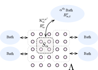
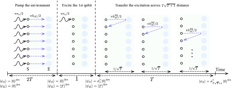
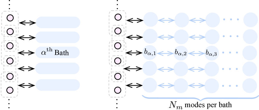
![[Uncaptioned image]](/html/2410.15481/assets/x4.png)
![[Uncaptioned image]](/html/2410.15481/assets/x5.png)
![[Uncaptioned image]](/html/2410.15481/assets/x6.png)